A pure variation of risk in …rst-price auctions

Oliver Kirchkamp, J. Philipp Reiss, Abdolkarim Sadrieh A pure variation of risk in private-value auctions RM/08/050 JEL code: C92, D44 Maastricht research school of Economics of TEchnology and ORganizations Universiteit Maastricht Faculty of Economics and Business Administration P.O. Box 616 NL - 6200 MD Maastricht phone : ++31 43 388 3830 fax : ++31 43 388 4873

A pure variation of risk in private-value auctions∗

Oliver Kirchkamp†, J. Philipp Reiss‡, Abdolkarim Sadrieh§

First version: March 1, 2006

This version: November 10, 2008

Abstract

We introduce a new method of varying risk that bidders face in first-price and second-price

private value auctions. We find that decreasing bidders’ risk in first-price auction reduces

the degree of overbidding relative to the risk-neutral Bayesian Nash equilibrium prediction.

This finding is consistent with the risk-aversion explanation of overbidding. Furthermore,

we apply the method to second-price auctions and find that bidding behavior is robust to

manipulating bidders’ risk as generally expected in auction theory.

Keywords: risk, first-price auctions, second-price auctions, risk-aversion, overbidding

JEL classification: C92, D44

∗We thank Dan Levin for stimulating comments. We also thank audiences in Atlanta (ESA 2006), Berlin,

Cologne, Evanston (Games 2008), Goslar, Jena, Maastricht, Munich, and Nottingham (ESA 2006) for helpful

comments. Financial support from the state Saxony-Anhalt is gratefully acknowledged.†University of Jena, [email protected]‡Maastricht University, [email protected]§University of Magdeburg, [email protected]

1

1 Introduction

Auction theory is a powerful economic tool. It is used to advise governments and businesses

on designing and bidding in auctions (e.g., Cramton, 1995, or Milgrom, 2004). In many cases,

however, auction designers and strategic advisors have complemented their auction theoretic

analysis with an experimental examination in order to check for the behavioral robustness of

the theoretic advice (e.g., Abbink et al., 2005, or McMillan, 1994). This additional information

evidently seems necessary because empirical and experimental research has uncovered systematic

discrepancies between observed and expected behavior in auctions. While numerous additions

to classical auction theory, especially alternative preference structures and stochastic choice

models, have been proposed in the literature, so far, no attempt has been made to quantify the

influence of any of the suggested effects. Hence, when an advisor is currently asked about the

state of the art in auction theory, the answer is rather unsatisfactory. It is well known that

classical auction theory is not fully in line with bidding behavior and it is also well known that

a number of phenomena may play a role. It is not known, however, to which degree any of the

suggested phenomena actually influence behavior.

In this paper we present a new experimental method that allows us to systematically quanti-

fying the influence of risk preferences on bidding behavior. Bidders’ non-neutral risk-preferences,

especially their risk-aversion,1 doubtlessly constitute one of the most prominent explanations of

the gap between observed and predicted bidding behavior (Kagel, 1995). While a number of

studies have demonstrated that risk-aversion alone is not sufficient to explain all deviations from

risk-neutral Bayesian Nash equilibrium prediction in first-price private value auctions,2 no study

has been able to completely rule out that risk-preferences may play a role in bidding behavior,

because ”one element of the theory that cannot be replicated in an experiment is the risk neu-

trality of bidders, for the risk attitudes of the subjects cannot be controlled.” (Andreoni et al.

2007, p. 246.)

The experimental protocol that we introduce allows us to control the amount of risk faced

by bidders in first- and second-price sealed-bid auctions with private values. Hence, instead

of measuring or inferring individual risk-preferences, we vary the risk in the auction situation

1The most widely propagated models of risk-averse bidders are the Constant Relative Risk-Aversion CRRA

Model (Cox et al., 1988) and the Constant Absolute Risk Aversion (CARA) Model (Maskin and Riley, 1984;

Matthews, 1987).2Most prominently perhaps, Kagel and Levin (1993) find overbidding relative to the risk-neutral prediction

in third-price auction experiments where risk-averse bidders are predicted to bid less than risk-neutral bidders.

Chen and Plott (1998) show that the CRRA model is outperformed by a simple model with linear markdowns, if

bidder’s values are not uniformly distributed as in most experiments. Kirchkamp and Reiss (2004) demonstrate

that - if not precluded by the experimental design - a substantial amount of underbidding for low valuations can

be observed, contradicting the notion of risk-averse bidders.

2

systematically for all bidders, no matter which risk-preferences they have. This opens up the

possibility to check to what extent risk-preferences explain bidding behavior and to what degree

other factors are relevant. Once risk is eliminated from the auction situation, any discrepancy

that remains between observed and predicted bidding cannot be attributed to risk-preferences.

If observed and predicted behavior are indistinguishable after eliminating the risk, then risk-

preferences seem to be sufficient to explain behavior. If discrepancies remain, we can establish

the relative importance of risk attitudes compared to the influence of other factors.3

Specifically, we isolate the effect of risk experienced by bidders in first-price and second-price

auctions in the presence of strategic uncertainty. We modify risk in a natural way by varying

the number of income-relevant auctions that a participant plays with a given bidding strategy

in each round. Our procedure is very different from the lottery payoff procedure that was first

introduced by Roth and Malouf (1979) and first used in auction experiments by Cox, Smith, and

Walker (1985). The lottery payoff procedure attempts to induce risk-neutral behavior by paying

subjects in lottery tickets for a final ”grand lottery.” Since only the chances to win, but not the

risk attached to the grand lottery is affected by the behavior in the experiment, expected utility

maximizers have risk-neutral preferences with respect to the lottery payment. Selten, Sadrieh,

and Abbink (1999), however, show that subjects’ choices using the method exhibit even greater

deviations from the risk-neutral behavior (and from expected utility maximization) than with a

standard payment procedure.4 The reason for the failure of the lottery payoff procedure seems

to be that subjects - in violation of the combined lottery reduction axiom - perceive the setup

as highly risky, because the payoff uncertainty is not dissolved gradually, but at once and only

after the final decision in the experiment. Our procedure avoids this problem, because there are

no combined lotteries and each choice is immediately followed by feedback after the round.

We find that the reduction of non-strategic risk moves observed bids significantly closer to

the risk-neutral Bayesian Nash equilibrium prediction in first-price auctions. Overbidding for

high valuations is significantly reduced, just as underbidding for low valuations. Hence, we have

clear evidence that risk-preferences matter in first-price auctions.

As a robustness test of our method to manipulate auction risk, we also consider second-

price private-value auctions. In second-price auctions, bidders have a weakly dominant bidding

strategy that is independent of risk considerations. We hypothesize that bidding behavior in

3Numerous other factors have been proposed in the literature that may affect bidding behavior. Morgan,

Steiglitz, and Reis (2003), for example, model spiteful bidding behavior. Selten and Buchta (1999), Ockenfels and

Selten (2005) and Neugebauer and Selten (2006) investigate the effect of information feedback and directional

learning. Crawford and Iriberri (2007) study the implications of level-k-thinking for auction settings. Engelbrecht-

Wiggans and Katok (2007a, forthcoming) and Filiz-Ozbay and Ozbay (2007) theoretically and experimentally

study the role of regret.4This, in fact, is well in line with the results of Cox, Smith, and Walker (1985).

3

these auctions is not affected by varying the level of risk. Indeed, we observe that reducing risk

does not affect bidding behavior in our second-price auction experiments. This result validates

our method and, thus, confirms our findings on the differentiated effect of risk-preferences on

bidding behavior in first-price auctions.

The plan of the paper is as follows: in section 2 we introduce the theoretical foundation for

eliminating risk in private-value first-price auctions. Section 3 describes our experimental design

and section 4 provides our main experimental findings. Section 5 concludes.

2 Theoretical considerations

2.1 Elimination of risk in first-price auctions

Consider a first-price auction with private values that are identically and independently dis-

tributed. In the Bayesian Nash equilibrium with a symmetric equilibrium bid function, bidders

face risky income prospects due to uncertainty about competitors’ private values. In this sub-

section we show that uncertainty of this type can be eliminated from the auction game inde-

pendently of arbitrary individual risk preferences. We transform the uncertain auction game

into a related auction game of certainty so that risk preferences become meaningless and players

behave as if risk neutral in the original game. Intuitively we achieve complete risk elimination

by averaging auction play over an infinite number of independent auction games where any

player’s strategy is fixed across all of these games while players’ private values are randomly

determined over and over again. In the limit players’ equilibrium payoffs are deterministic and

equal to expected equilibrium payoffs of the game played only once with risk neutral preferences.

Theorem 1 formalizes the intuition.

Theorem 1. Let β(v) denote the symmetric equilibrium bid function in Bayesian Nash equi-

librium under risk neutrality in the standard one-shot first-price auction game Γ. Let Σ(m)

denote a new auction game with individual von Neumann-Morgenstern risk preferences where

each player bids with a fixed bidding strategy in m > 1 independent shots of the standard auc-

tion game Γ such that any player’s payoff in auction game Σ(m) is given by the average gain

obtained in all m one-shot auctions. For m → ∞, the strategy profile in symmetric Bayesian

Nash equilibrium with risk neutrality in the standard auction game Γ is a symmetric Bayesian

Nash equilibrium strategy profile in game Σ(m → ∞) with arbitrary individual risk preferences.

Proof. Consider a standard private-value first-price auction with n bidders each having arbitrary

von Neumann-Morgenstern risk preferences. The utility function of a representative player 1

is denoted by u1(·) such that u′1 > 0 and u1(0) = 0. Assume that players’ random values,

~V = (V1, ..., Vn), are independently and identically distributed according to a probability density

4

function f(v) with domain D. Let X1(~V ) denote player 1’s random gain from the auction given

that all players adhere to bidding strategy profile ~b = (b1(V1), ..., bn(Vn)). By independently

distributed values, player 1’s expected auction gain can be written as

E[X1(~V )] =

∫

D

f(v1)E[X1(~V )|V1 = v1] dv1.

According to the rules of the first-price auction, the high-bidder wins the auction and pays her

bid implying E[X1(~V )|V1 = v1] = Pr{bid b1(v1) wins} [v1 − b1(v1)], therefore,

E[X1(~V )] =

∫

D

f(v1) Pr{bid b1(v1) wins} [v1 − b1(v1)] dv1.

Now suppose that all players bid according to strategy profile ~b not only in a single auction

but in m different standard one-shot auctions where for each player m values are independently

drawn, a new one for each of m one-shot auctions. Further, assume that any player’s payoff is

equal to the average gain obtained in all m one-shot auctions. The average gain of player 1 is

denoted by W1(·) and given by

W1(~V1, ..., ~Vm) =

∑mj=1 X1,j(~Vj)

m.

The average gain W1(·) is computed from a series of m independently and identically distributed

random variables. Therefore, the law of large numbers is applicable and implies that average

gain W1(·) is deterministic in the limit, equalling expected value E[X1(·)]:

limm→∞

W1(~V1, ..., ~Vm) =

∫

D

f(v1) Pr{bid b1(v1) wins} [v1 − b1(v1)] dv1. (1)

The maximization problem of player 1 when participating in m one-shot auctions with bidding

strategy b1(·) and receiving the average gain as payoff is given by

maxb1(v1)

EU[W1(~V1, ..., ~Vm)].

As the number of auctions approaches infinity, result (1) implies that the maximization problem

simplifies to

maxb1(v1)

EU[E[X1(·)]] = u1

(∫

D

f(v1) Pr{bid b1(v1) wins} [v1 − b1(v1)] dv1

)

. (2)

Since the utility function is upward-sloping, maximization problem 2 is solved by the same

bidding strategy that also solves, for any value v1 ∈ D, the following set of maximization

problems, each conditional on v1:

maxb1

Pr{bid b1 wins} [v1 − b1].

Since the preceding problem is the standard maximization problem faced in a single private-value

first-price auction with risk-neutral preferences, it is shown that the equilibrium strategy profile

in standard auction game Γ with risk-neutrality is an equilibrium strategy profile in auction

game Σ(m → ∞) with with arbitrary risk-preferences.

5

Corollary 1. If each player’s utility function is characterized by constant relative risk aversion,

i.e. ui(x) = xri , theorem 1 extends to the case where any player i’s payoff in game Σ(m) is the

sum of gains player i obtains in the m one-shot auctions.

For risk-preferences consistent with, possibly heterogeneous, constant relative risk aver-

sion (CRRA), corollary 1 extends the theorem to the case where any player’s average payoff

is replaced by the sum of gains in all individual one-shot auctions.

We proceed by illustrating how the equilibrium bid strategy in auction game Σ(m) ap-

proaches the equilibrium bid strategy prevailing in the limit (which is identical to the risk-neutral

equilibrium bid strategy) if the number of one-shot auction games m is varied.

2.2 First-price auctions with reduced risk

Total elimination of risk relies on the assumption of playing infinitely many auction games. Of

course, there are limits to infinity in auction experiments if players are informed about each

individual outcome in the series of auction games. Otherwise it might be sufficient to pay

the expected value to incorporate infinity into the auction setting as, e.g., in the rent-seeking

experiment of Vogt, Weimann, and Yang (2002). This, however, requires that the implications

of this procedure are transparent to subjects.

If bidders use their bidding strategies in a finite number of auctions, situations with inter-

mediate risk arise that lie between full risk in a single auction and completely eliminated risk

in infinitely many auctions. The uncertain income prospect can be gradually varied by varying

the number of auctions in which each bidding strategy is used.

To illustrate the idea of gradually varying risk, suppose that it is common knowledge that

valuations x are uniformly and independently distributed over [0, 1]. Assume that utility func-

tions have the form of u(x) = xr where r is the parameter measuring attitude towards risk.5 A

risk-neutral individual is described by r = 1, a risk-averse individual is characterized by r < 1.

To identify a Bayesian Nash equilibrium we follow the standard approach and assume that there

is a symmetric and strictly increasing bid function β(x). In equilibrium, all bidders follow a

bid function β(x). For the case of two bidders, we have to show that if bidder 2 follows β(x),

then it is a best reply for bidder 1 to follow β(x), too. Since β(x) is strictly increasing, we

can identify for each bid b a valuation z such that b = β(z). Bidder 1 wins the auction if the

other bidder’s valuation is smaller than z. The probability of this event is F (z) = z. If the

bidder plays m auctions with the same bid function, the bidder wins k of these auctions with

5Smith and Walker (1993) report that upward scaling the conversion rate at which laboratory currency is

converted into cash has an insignificant effect on mean bid deviations from risk-neutral equilibrium bids. The

utilized utility function is the only functional form satisfying scale independence of payoffs.

6

probability(

mk

)

· F (z)k · [1 − F (z)]m−k. Bidder 1 maximizes

EU =

m∑

k=0

(

m

k

)

· F (z)k · [1 − F (z)]m−k · u[k · (x − β(z)]

For a symmetric equilibrium it is necessary that we have ∂EU/∂z = 0 and z = x. Given constant

relative risk-aversion (u(x) = xr) it is straightforward to solve the corresponding differential

equation for the case m = 1. With β(0) = 0 we obtain the well-known equilibrium bid function

β∗(x) = x/(1+ r). For m = 2 it is possible to find a closed-form solution. For m > 2 we have to

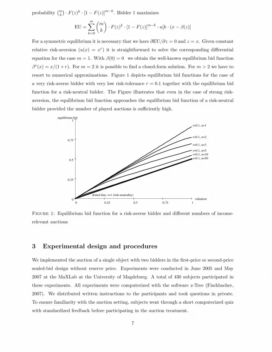
resort to numerical approximations. Figure 1 depicts equilibrium bid functions for the case of

a very risk-averse bidder with very low risk-tolerance r = 0.1 together with the equilibrium bid

function for a risk-neutral bidder. The Figure illustrates that even in the case of strong risk-

aversion, the equilibrium bid function approaches the equilibrium bid function of a risk-neutral

bidder provided the number of played auctions is sufficiently high.

10.750.50.250

1

0.75

0.5

0.25

0

equilibrium bid

valuation

r=0.1, n=1

r=0.1, n=2

r=0.1, n=3

r=0.1, n=5

r=0.1, n=10

r=0.1, n=50

dotted line: r=1 (risk-neutrality)

Figure 1: Equilibrium bid function for a risk-averse bidder and different numbers of income-

relevant auctions

3 Experimental design and procedures

We implemented the auction of a single object with two bidders in the first-price or second-price

sealed-bid design without reserve price. Experiments were conducted in June 2005 and May

2007 at the MaXLab at the University of Magdeburg. A total of 430 subjects participated in

these experiments. All experiments were computerized with the software z-Tree (Fischbacher,

2007). We distributed written instructions to the participants and took questions in private.

To ensure familiarity with the auction setting, subjects went through a short computerized quiz

with standardized feedback before participating in the auction treatment.

7

Round: 1 of 12 Remaining time [sec]: 113

You receive 0 ECU if you make the smallest bid in an auction

The other bidder receives 0 ECU if he makes the smallest bid in the auction

Your valuation will be a number between 50 and 100

The valuation of the other bidder will be a number between 50 and 100.

0

10

20

30

40

50

60

70

80

90

100

110

50 60 70 80 90 100

Valuation [ECU]

Bid [ECU]

b

b

b

b

b

b

Please indicate your bid function depending

on the valuation that is still going to be

determined

For a valuation of 50 ECU I bid: 46.6



For a valuation of 80 ECU I bid: 76



Draw bids

Finish input stage

Figure 2: A typical input screen in the experiment (hypothetical data, translated into English)






0

10

20

30

40

50

60

70

80

90

100

110

120

Valuation: 50 60 70 80 90 100

Bid [ECU]

b

b

b

b

bb

value bid gain

∗1) 50.69 50.35 -

∗2) 51.00 50.50 -

∗3) 53.91 51.95 -

∗4) 53.99 52.00 -

∗5) 54.88 52.44 -

∗6) 56.22 53.11 -

∗ 7) 56.45 53.23 3.23

∗8) 57.90 53.95 -

∗9) 58.30 54.15 -

∗10) 58.73 54.36 -

∗11) 59.41 54.70 -

∗12) 59.58 54.79 -

∗13) 60.03 55.02 5.02

∗14) 61.59 55.80 -

∗15) 61.89 55.95 -

∗16) 61.98 55.99 5.99

∗17) 63.38 56.69 -

∗18) 63.82 56.91 -

∗19) 66.23 58.12 -

∗20) 66.27 58.13 -

∗21) 67.37 58.69 -

∗22) 68.70 59.35 -

∗23) 69.28 59.64 9.64

∗24) 69.34 59.67 -

∗25) 70.84 60.42 -

value bid gain

∗26) 73.03 61.51 11.51

∗27) 73.35 61.68 -

∗28) 74.93 62.47 12.47

∗29) 74.97 62.48 12.48

∗30) 77.30 63.65 -

∗31) 77.33 63.67 -

∗32) 77.99 64.00 14.00

∗33) 78.79 64.39 14.39

∗34) 78.97 64.48 -

∗35) 79.27 64.64 -

∗36) 79.71 64.86 14.86

∗37) 79.89 64.94 14.94

∗38) 79.96 64.98 14.98

∗39) 82.18 66.09 -

∗40) 89.53 69.76 19.76

∗41) 90.49 70.24 20.24

∗42) 91.59 70.79 20.79

∗43) 91.82 70.91 20.91

∗44) 93.83 71.91 21.91

∗45) 96.30 73.15 23.15

∗46) 96.43 73.21 23.21

∗47) 96.49 73.25 23.25

∗48) 97.41 73.71 23.71

∗49) 97.94 73.97 23.97

∗50) 98.16 74.08 24.08

Figure 3: A typical feedback screen in the experiment (A50G50FP, hypothetical data)

8

Strategy method In the experiments we employed the strategy method to elicit bid functions.

Selten and Buchta (1999) introduced the strategy method to experimental auctions. Subsequent

studies, e.g., Pezanis-Christou and Sadrieh (2004) and Guth et al. (2002, 2003), applied it

to various auction settings and obtained bidding data that assure the reliability of the more

complex method of eliciting entire bid functions as opposed to eliciting a single bid for an

assigned valuation. Our implementation of the strategy method follows Kirchkamp, Poen and

Reiss (forthcoming). In particular, we required participants to specify their bids for six different

valuations (50, 60, ..., 100). Bids for valuations that were between those six valuations were

obtained by linear interpolation. Figure 2 displays a typical input screen that participants

faced to submit their bidding strategy in each round. This method to submit bidding strategies

remained unchanged across all rounds and treatments.

Table 1: Treatment information

number of income- number of first- second- number of number of

relevant auctions displayed auctions price price independent subjects

treatment (A) (G) (FP) (SP) observations

A1G50FP 1 50 yes 6 54

A50G50FP 50 50 yes 6 56

A1G50SP 1 50 yes 9 72

A50G50SP 50 50 yes 9 72

control treatment

A1G1FP 1 1 yes 6 48

A10G50FP 10 50 yes 6 56

A1G1SP 1 1 yes 9 72

Treatments In order to explore the role of risk preferences in private-value auctions, we

consider three treatment variables: the number of income-relevant auctions (A), the number of

auctions whose outcome is displayed to participants as feedback (G), and the auction format

which is either first-price (FP) or second-price (SP). Table 1 summarizes parameter details of

each treatment.

Each treatment was divided into twelve rounds. In each round each participant was randomly

matched with one other participant and used the submitted bidding strategy against her matched

competitor in a fixed number of auction games. The number of played auction games per round

was either one or fifty depending on the treatment. For every single auction game in any round,

the valuation assigned to each participant was independently drawn from a uniform distribution

with domain [50, 100]. A subset of all displayed auction games was selected at random to

determine round income as the sum of all gains in the corresponding individual auction games.

The number of selected auctions that was relevant for income determination was either one or

9

fifty; in control-treatment A10G50FP there were ten income-relevant auctions. If an auction

outcome was selected as income-relevant, it was marked with an asterisk in the feedback screen.

Multiple feedback on auction outcomes Figure 3 illustrates a typical feedback screen

used in treatment A50G50FP where participants played 50 different auction games per round.

The outcomes in all of these auctions were used to compute round income. Analogously, in the

treatments with one income-relevant auction where 50 auctions were played, a single auction

game was randomly selected and its outcome determined total round income. Figure 4 shows a

typical feedback screen used in treatment A1G1FP with a single auction game played per round.






0

10

20

30

40

50

60

70

80

90

100

110

120

Valuation: 50 60 70 80 90 100

Bid [ECU]

b

b

b

b

bb

value bid gain

∗ 1) 56.45 53.23 3.23

Figure 4: A typical feedback screen in the experiment (treatment A1G1FP, hypothetical data)

4 Experimental results

In this section we provide our main experimental results. Firstly, section 4.1 presents the effects

of manipulating risk on bidding behavior in first-price and second-price auctions. Secondly,

in section 4.2, we report how bidding behavior responds to extensive variations of feedback.

Thirdly, section 4.4 argues that the choice of 50 income-relevant auctions is a conservative one

for our subjects to perceive the auction setting as free of risk.

All results reported in section 4 use data from the entire experiment. Typically the first few

rounds of auction experiments are characterized by particularly strong fluctuations of bidding

activity. In response we investigate bidding dynamics over time and find that our main results

are robust to them, see appendix A.1. In appendix A.2 we complement the subset of our main

10

results given on the aggregate level with an examination on the individual level suggesting

robustness also to this end.

4.1 The effects of reducing risk

Most importantly, we manipulated risk that bidders face in auctions. We essentially eliminated it

by increasing the number of auctions that a bidder played with the same bidding strategy against

the same opponent, but with different draws of the own and the opponent’s valuations. The

outcomes of a subset of all of these played auctions determined the round income of participants.

Irrespective of the auction rule, first-price or second-price, in treatments A1G50 and A50G50

every participant played 50 auctions in each round of the experiment with the same bidding

strategy. In treatment A1G50 a single auction out of 50 played auctions was selected at random.

The outcome of the selected auction entirely determined the participant’s round income. In

contrast, in treatment A50G50 all 50 auctions were selected to determine the participant’s

round income. Evidently, risk is much smaller if 50 different auction outcomes based on 50

different own and opponent’s valuations determine round income instead of exclusively hinging

on a single outcome.

4.1.1 First-price auctions

Under the first-price rule in Bayesian Nash equilibrium, any decrease of risk induces risk-averse

bidders to bid closer to the risk-neutral equilibrium bid function. If risk entirely disappears, even

a very risk-averse bidder bids as if having risk-neutral preferences by specifying the risk-neutral

equilibrium bid function. Consequently, the theoretical predictions for risk-averse equilibrium

in the reduced risk treatment (A50G50FP) are closer to risk-neutral equilibrium than in the

standard risk treatment (A1G50FP). Therefore, if overbidding is due to risk aversion, we should

expect more overbidding in the standard risk treatment (A1G50FP) than in the treatment with

reduced risk (A50G50FP).

In our experiments we observe bid functions as opposed to single bids. This allows us to

measure overbidding on the entire valuation domain. To quantify overbidding we use the area

between the observed bid function and the risk-neutral equilibrium bid function. This concept

naturally extends the standard approach of measuring overbidding as the difference of observed

bid and risk-neutral equilibrium bid to the case of bid functions. Following the conventional

approach, we ignore bids smaller than the risk-neutral prediction when studying overbidding.

Therefore, our overbidding measure of bidder i in round t is given by:

A+i,t(bi,t, β

RNBNE) =

∫ 100

50max{0, bi,t(v) − βRNBNE(v)} dv,

For interpreting values of area measure A+, note that infinite risk-aversion, i.e. b(v) = v, leads

11

to A+ = 625 ECU; (it equals 50 ECU if observed bids exceed risk-neutral equilibrium bids by

1 ECU for any valuation v.)

The left panel of Figure 5 shows histograms of individual overbidding in the first-price treat-

ments with reduced risk (dark bars) and standard risk (light bars) using overbidding measure

A+i,t; the right panel depicts corresponding cumulative distribution functions. There is a large

0

10

20

30

40pe

rcen

t

0 − 125 125 − 250250 − 375 > 375

Area b/w individual bid function and RNBNE

Reduced risk (A50G50FP)

Standard risk (A1G50FP)

A1G50FPA50G50FP

0

.2

.4

.6

.8

1

cum

ulat

ed r

elat

ive

freq

uenc

y0 200 400 600




Figure 5: Overbidding response in first-price auctions when reducing risk

amount of overbidding in the standard risk treatment where the individual area measures of

overbidding range from 0 to 569.17 ECU. With standard risk, 70.4% of bidders exhibit an over-

bidding measure larger than 250 ECU. In contrast, large overbidding of this magnitude applies

to only 35.7% of bidders in the reduced risk treatment. Further, in the standard risk treatment,

there are 35.2% of bidders with overbidding measures exceeding 375 ECU while there are only

7.1% of bidders showing similarly large overbidding in the reduced risk treatment. The lower

frequency of large overbidding in the reduced risk treatment is reflected in the higher frequency

of small amounts of overbidding; in the standard risk treatment only 29.3% of bidders exhibit

an overbidding measure smaller than 250 ECU while there are 64.3% of bidders with a similarly

small overbidding measure in the reduced risk treatment. Evidently, reducing risk shifts mass

of the overbidding distribution to the left so that there is less overbidding with less auction

risk. A Kolmogorov-Smirnov test confirms significant differences between both distributions

(p = 0.026). We apply this and all other tests (including the t-test) on averages on indepen-

dent observation level. Summary statistics for the area measure of overbidding are provided in

Table 7 in the appendix.

12

To quantify the amount of overbidding that is attributable to the risk-aversion hypothesis,

we regress the amount of overbidding A+ on a constant and a treatment dummy Drr following

equation (3) for treatments A1G50FP and A50G50FP. The dummy variable indicates if the

observation was in the reduced risk treatment (Drr = 1) or in the standard risk treatment

(Drr = 0). Calculations of standard errors are robust and take into account that observations

might be correlated within matching groups but not across matching groups (Rogers, 1993).

Results are summarized in Table 2.

A+i,t = βo + βDDrr

i,t + ui,t (3)

According to the regression results, our area measure of overbidding is 336.9 ECU with standard

risk. As soon as risk is eliminated from the auction setting, overbidding falls by 135.6 ECU.

Hence, the risk-aversion hypothesis explains 40.3% of overbidding in our standard risk treatment

(A1G50FP); this is significantly different from zero (two-tailed t-test. p = 0.002).

explanatory variable coefficient β robust σβ t P > |t|

constant 336.930 25.424 13.25 0.000

Drr -135.566 33.280 -4.07 0.002

Table 2: Estimation of equation (3)

Finding 1. Reducing risk in first-price private value auctions leads to less overbidding relative

to risk-neutral Bayesian Nash equilibrium, supporting the risk-aversion hypothesis.

Next we consider the impact of reducing risk on the average bid function to explore whether

overbidding reductions are of local or global nature. For comparison of aggregate bidding be-

havior in the experiment and the risk-neutral equilibrium benchmark, consider the left panel of

Figure 6. It depicts the average bid functions observed in the first-price treatments with standard

risk (A1G50FP) and reduced risk (A50G50FP) together with the risk-neutral equilibrium bid

function.6 As can be seen, the average bid function in the standard risk treatment (A1G50FP)

is above the risk-neutral equilibrium bid function except for small valuations. This indicates

that our collected first-price data for standard risk share the robust findings of underbidding for

small valuations and overbidding for the residual set of valuations reported elsewhere; e.g., Cox

et al. (1982), Kagel, Harstad and Levin (1987), Kagel (1995), Guth et al. (2003), and Kirchkamp

and Reiss (2004).

Importantly, the average bids presented in the left panel of Figure 6 and detailed in Table 3

show that increasing the number of income-relevant auctions from 1 to 50 shifts the average bid

6Average bids are computed as the average of bids over the respective independent observations and the total

number of periods.

13

45°

reduced risk

RNBNE

standard risk

50

60

70

80

90

100

aver

age

bid

50 60 70 80 90 100

valuation

round income earned in 1 auction

round income earned in 50 auctions

risk−neutral Bayesian Nash eq.

standard risk(A1G50FP)

reduced risk(A50G50FP)

0

.2

.4

.6

.8

1

cum

ulat

ed r

elat

ive

freq

uenc

y

0 200 400 600

absolute deviation from risk−neutral BNE



Figure 6: Bidding strategy effect in the experiment if the number of auctions played with the

same bidding strategy increases under the first-price auction format.

Left panel: Average bid functions. Right panel: Cumulative frequencies of individual absolute deviations

from risk-neutral equilibrium Ai,t.

function downward so that bidding is less aggressive with reduced risk. The effect of smaller

bids with less risk is statistically significant.7

The effect of reduced risk on absolute deviations from risk-neutral equilibrium as shown in

Figure 6 is ambiguous. On the one hand, underbidding for small valuations appears to increase

with reduced risk so that deviations ceteris paribus increase. On the other hand, the reduction of

overbidding ceteris paribus reduces deviations. We quantify the individual net effect of reduced

risk on risk-neutral equilibrium deviation as the area between any observed bid function for

bidder i in period t and the risk-neutral equilibrium function:

Ai,t(bi,t, βRNBNE) =

∫ 100

50| bi,t(v) − βRNBNE(v) | dv.

The last column of Table 3 provides the average distance between bid functions observed in the

first-price treatments and the risk-neutral equilibrium prediction using area measure Ai,t. With

7This is revealed by comparisons of average bids in the standard risk treatment (A1G50FP) to those in the

reduced risk treatment (A50G50FP) using non-parametric Mann-Whitney-U -tests separately for each valuation

(two-tailed, p ≤ 0.0374); similarly, t-tests identify significant differences of average bids across treatments (two-

tailed, p ≤ 0.0292).

14

Table 3: Average bids in the first-price auction

valuation 50 60 70 80 90 100 A(b, βRNBNE)

βRNBNE 50.0 55.0 60.0 65.0 70.0 75.0 0.0

A1G50FP 46.1 55.1 63.8 72.0 80.4 88.5 356.3

(1.10) (1.42) (1.99) (2.74) (2.78) (2.81) (63.52)

A50G50FP 43.8 52.6 60.8 68.2 75.9 83.0 271.9

(1.85) (2.00) (1.87) (2.24) (2.29) (2.53) (31.10)

Note: Standard deviations in parenthesis.

less risk (A50G50FP) observed bid functions are significantly closer to the risk-neutral prediction

so that there are less deviations overall (two-tailed Mann-Whitney-U -test, p = 0.0374; two-tailed

t-test, p = 0.0153).

Further, the right panel of Figure 6 depicts cumulative distributions of individual absolute de-

viation averaged over rounds for treatments A1G50FP and A50G50FP using area measure Ai,t.

It can readily be seen that increasing the number of income-relevant auctions shifts the cu-

mulated frequencies to the left implying substantially less deviations and less overbidding. A

Kolmogorov-Smirnov test on the level of independent observations confirms that both distribu-

tions are significantly different from one another (p = 0.026). Reducing risk moves observed bid

functions closer to risk-neutral equilibrium.

Finding 2. Reducing risk in first-price private value auctions leads to smaller bids and less

deviations from risk-neutral Bayesian Nash equilibrium.

4.1.2 Second-price auctions

In the second-price auction, the symmetric equilibrium bidding strategy is not affected by ma-

nipulations of risk since it is weakly dominant, βSP(v) = v. Therefore, we hypothesize to observe

no difference in bidding behavior between the standard risk treatment (A1G50SP) and the re-

duced risk treatment (A50G50SP). Figure 7 illustrates data for the second-price treatments

with standard risk (A1G50SP) and reduced risk (A50G50SP). The left panel presents average

bid functions. The right panel depicts cumulative distributions of individual deviations of ob-

served bidding strategies from the weakly dominant equilibrium strategy using area measure Ai,t.

In contrast to our first-price treatments, we do not find a treatment effect of average bids with

reduced risk. For small valuations, average bids in the standard risk treatment (A1G50SP) are

smaller than in the reduced risk treatment (A50G50SP), for larger valuations there is either no

visible difference between average bids or the average bid in the standard risk treatment is larger.

Table 4 summarizes data on average bids. Testing for treatment effects of average bids condi-

15

reduced risk

standardrisk

50

60

70

80

90

100

110

aver

age

bid

50 60 70 80 90 100

valuation



weakly dominant strategy

standard risk(A1G50SP)

reduced risk(A50G50SP)

0

.2

.4

.6

.8

1

cum

ulat

ed r

elat

ive

freq

uenc

y

0 500 1000 1500

absolute deviation from dominant strategy



Figure 7: Bidding strategy effect in the experiment if the number of auctions played with the

same bidding strategy increases under the second-price auction format.

Left panel: Average bid functions. Right panel: Cumulative frequencies of individual absolute deviations

from weakly dominant strategy Ai,t.

tional on valuation does not reveal significant differences (two-tailed Mann-Whitney-U -tests,

p ≥ 0.2697; two-tailed t-tests, p ≥ 0.2195).

The average bid functions depicted in Figure 7 and the data given in Table 4 indicate that

our data are characterized by widespread overbidding in the sense of bids exceeding valua-

tions. This finding is widely documented for second-price auctions, though not conclusively

understood, see, e.g., Andreoni, Che and Kim (2007), Cooper and Fang (forthcoming), Guth et

al. (2003), Kagel (1995), Kagel, Harstad and Levin (1987), Kagel and Levin (1993), and Garratt,

Walker and Wooders (2004). Interestingly, our results are inconsistent with possible risk-based

explanations of overbidding in second-price auctions since the level of risk appears not to be a

major determinant of bidding behavior: The areas between individual bidding strategies and the

weakly dominant strategy observed in both treatments (last column of Table 4) do not statis-

tically differ from one another (two-tailed Mann-Whitney-U -test, p = 0.8946; two-tailed t-test,

p = 0.9297). Further, the treatment distributions of individual absolute deviations between

equilibrium and observed bidding strategies virtually coincide as the right panel of Figure 7

shows. Here, a Kolmogorov-Smirnov test on the independent observation level fails to identify

16

Table 4: Average bids in the second-price auction

valuation 50 60 70 80 90 100 A(b, βWDS)

βWDS 50.0 55.0 60.0 65.0 70.0 75.0 0.0

A1G50SP 54.9 64.8 74.5 84.8 94.4 102.6 313.02

(5.80) (5.18) (4.79) (4.83) (4.80) (6.56) (183.09)

A50G50FP 51.7 62.2 72.5 83.8 95.4 107.0 322.22

(5.00) (3.95) (4.16) (4.85) (8.25) (9.35) (247.49)


significant differences (p = 0.730).

Finding 3. Reducing risk in second-price private value auctions does not affect bidding behav-

ior. The empirical regularity of overbidding valuations in second-price auctions is robust to

manipulations of risk.

4.2 The effects of information feedback about multiple auction outcomes

The standard first-price or second-price auction experiment informs individual bidders about

the outcome of a single auction after bidding with an assigned private value and before bidding

with a newly assigned private value in the next round of the experiment. Although learning

opportunities are limited with repeated single bid-value experiences, bidding behavior is found

to respond.8 Nevertheless, outcome feedback does not reduce deviations from the risk-neutral

equilibrium prediction, neither in first-price nor second-price auctions.9

In comparison to single outcome feedback in any round, our feedback on 50 different auc-

tion outcomes for a given pair of bidders with fixed bidding strategies is extensive. It provides

participants with ample opportunities to assess the consequences of multiple bid-value combi-

nations where values are distributed over the entire valuation domain at the same time. Since

the amount of feedback given in our treatments substantially differs from traditional feedback

conditions we investigate if our findings regarding the effects of risk manipulation are robust to

extensive feedback.

8Experimental studies analyzing the effects of information feedback include Isaac and Walker (1985), Selten

and Buchta (1999), Guth et al. (2003), Ockenfels and Selten (2005), Brosig and Reiss (2007), and Engelbrecht-

Wiggans and Katok (forthcoming).9See, in particular, Guth et al. (2003) exporing learning effects in first-price and second-price auctions.

17

singlefeedback

extensivefeedback

RNBNE

50

60

70

80

90

100

aver

age

bidd

ing

func

tions

50 60 70 80 90 100

valuation

feedback: 1 auction

feedback: 50 auctions

RNBNE

extensivefeedback

(A1G50FP)

singlefeedback(A1G1FP)

RN

BN

E

0

.2

.4

.6

.8

1

cum

ulat

ed r

elat

ive

freq

uenc

y

35 40 45 50

bid distribution for v=50

feedback: 1 auction


singlefeedback(A1G1FP)

extensivefeedback

(A1G50FP)

RN

BN

E

0

.2

.4

.6

.8

1

cum

ulat

ed r

elat

ive

freq

uenc

y

70 80 90 100

bid distribution for v=100

feedback: 1 auction


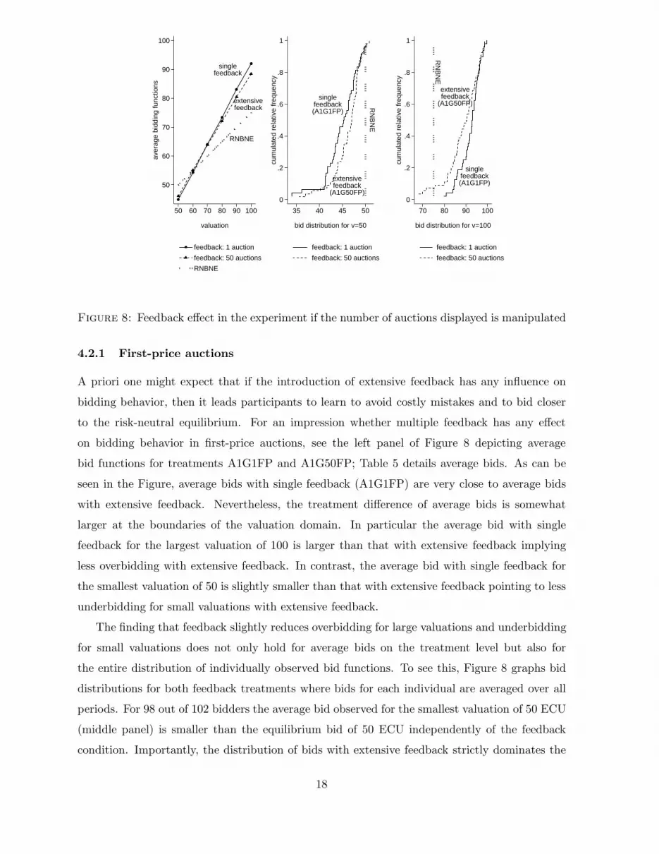
Figure 8: Feedback effect in the experiment if the number of auctions displayed is manipulated

4.2.1 First-price auctions

A priori one might expect that if the introduction of extensive feedback has any influence on

bidding behavior, then it leads participants to learn to avoid costly mistakes and to bid closer

to the risk-neutral equilibrium. For an impression whether multiple feedback has any effect

on bidding behavior in first-price auctions, see the left panel of Figure 8 depicting average

bid functions for treatments A1G1FP and A1G50FP; Table 5 details average bids. As can be

seen in the Figure, average bids with single feedback (A1G1FP) are very close to average bids

with extensive feedback. Nevertheless, the treatment difference of average bids is somewhat

larger at the boundaries of the valuation domain. In particular the average bid with single

feedback for the largest valuation of 100 is larger than that with extensive feedback implying

less overbidding with extensive feedback. In contrast, the average bid with single feedback for

the smallest valuation of 50 is slightly smaller than that with extensive feedback pointing to less

underbidding for small valuations with extensive feedback.

The finding that feedback slightly reduces overbidding for large valuations and underbidding

for small valuations does not only hold for average bids on the treatment level but also for

the entire distribution of individually observed bid functions. To see this, Figure 8 graphs bid

distributions for both feedback treatments where bids for each individual are averaged over all

periods. For 98 out of 102 bidders the average bid observed for the smallest valuation of 50 ECU

(middle panel) is smaller than the equilibrium bid of 50 ECU independently of the feedback

condition. Importantly, the distribution of bids with extensive feedback strictly dominates the

18

distribution with single feedback (in the sense of stochastic first-order dominance) so that there

is less underbidding with extensive feedback. In contrast, the right panel of Figure 8 indicates

that the distribution of bids for the largest valuation of 100 ECU with single feedback dominates

that for bids with extensive feedback so that there is less overbidding with extensive feedback

for any bidder participating in our experiments. Interestingly, extensive feedback leads a few

bidders to submit bids below the equilibrium bid for a value of 100 ECU which we did not

observe with single feedback.

To rigorously test for treatment-wise differences between average bids for any given valuation,

we employ Mann-Whitney-U -tests. We find that average bids significantly differ only for the

large boundary valuations 90 and 100 ECU (two-tailed, p ≤ 0.0782). For the smallest boundary

valuation 50, the Mann-Whitney-U test slightly misses weak significance (p = 0.1093)10 , it

clearly misses significance (p ≥ 0.2623) for the valuations 60,70 and 80. If we apply two-tailed

t-tests to our data, we find significant differences of average bids for the smallest valuation 50

and the largest valuations 90 and 100 (p ≤ 0.0844); all other differences of average bids are

insignificant (p ≥ 0.2713). Taken together extensive feedback slightly rotates the average bid

function.

Table 5: Average bids in the first-price auctions by treatment

valuation 50 60 70 80 90 100 A(b, βRNBNE)

βRNBNE 50.0 55.0 60.0 65.0 70.0 75.0 0.0

A1G1FP 44.9 54.4 64.0 73.4 83.0 92.0 393.9

(1.07) (1.07) (1.10) (1.08) (1.70) (1.79) (37.00)

A1G50FP 46.9 55.1 63.8 72.0 80.4 88.5 356.2

(1.10) (1.42) (1.99) (2.74) (2.78) (2.81) (63.52)


We proceed by investigating if the rather weak effect of feedback significantly reduces global

deviations from risk-neutral equilibrium. To this end, we measure the distance between observed

average bid functions and the risk-neutral equilibrium bid function using the area measure of

absolute deviations, see the last column of Table 5. Apparently there are less deviations with

extensive feedback. Extensive feedback closes roughly 10% of deviations observed with single

feedback. Nevertheless, neither the t-test (two-tailed, p = 0.2385) nor the Mann-Whitney-U -test

(two-tailed, p = 0.3367) identifies a significant feedback effect on deviations from risk-neutral

Bayesian Nash equilibrium; further, the finding of insignificant differences between both feedback

10If we control for learning in the early periods of the experiment and restrict our data set to the second half

of the experiment, this difference is significant (p = 0.025).

19

treatment is supported by a Kolmogorov-Smirnov test (p = 0.474). Taken together, the evidence

suggests that extensive feedback on multiple auction outcomes is, here, a secondary determinant

of bidding behavior. We conclude that our results on the manipulation of risk in first-price

auctions are not distorted by the introduction of extensive feedback into the standard auction

setting.

Finding 4. The introduction of extensive feedback on multiple auction outcomes does not sub-

stantially affect bidding behavior in first-price auctions. Extensive feedback slightly rotates the

average bid function so that that there are less deviations from Bayesian Nash equilibrium with

extensive feedback.

4.2.2 Second-price auctions

For the case of first-price auctions, we observed a weak effect of extensive feedback on average

bids at the boundaries of valuation domain. For second-price auctions, there emerges no feedback

effect at all at the level of independent observations. This might be due to the fact that feedback

is provided for multiple auction outcomes spread over the entire valuation domain where there

are typically always some auctions won by any participant while others are lost so that, from the

point of Learning Direction Theory (see Selten and Buchta, 1999, Guth et al., 2003), there is no

obvious direction for bid adjustment. Table 6 provides average bids conditional on valuations

for our second-price treatments with varied feedback condition. Although average bids observed

Table 6: Average bids in the second-price auctions by treatment

valuation 50 60 70 80 90 100 A(b, βWDS)

βWDS 50 60 70 80 90 100 0.0

A1G1SP 53.9 63.6 73.1 82.7 92.3 101.8 324.1

(3.89) (4.26) (4.39) (4.27) (4.26) (4.55) (152.5)

A1G50SP 54.9 64.8 74.5 84.8 94.4 102.6 313.0

(5.80) (5.18) (4.79) (4.83) (4.80) (6.56) (183.1)


with extensive feedback (A1G50SP) are roughly 1 ECU larger than those observed with standard

feedback (A1G1SP), there is no significant difference in any of the statistical comparisons of

average bids separately for each valuation (two-tailed Mann-Whitney-U test: p > 0.452; two-

tailed t-tests: p > 0.341). In both treatments we observe overbidding of the weakly dominant

strategy βWDS reflecting the standard finding for second-price auction experiments in our data.

Given no differences between average bids across treatments, it is not surprising that there is

no significant difference of global deviations from the weakly dominant strategy and the average

20

bid function between both feedback treatments (two-tailed Mann-Whitney-U test: p > 0.825;

two-tailed t-tests: p > 0.893). Again we employ the area between the average bid function and

the equilibrium bid function, A(b, βWDS), to measure global deviations between the average bid

function and the weakly dominant strategy (WDS).

4.3 Feedback absorption, complexity, and auction format

The second-price auction may be viewed as less complex for bidders due the existence of a weakly

dominant strategy that allows bidders to ignore strategic considerations regarding competitors

such as, e.g., the value distribution, inaccurate expectations, or suboptimal response behavior

to held expectations. In contrast to standard feedback where a single auction experience is

provided, our extensive feedback treatments (A1G50FP and A1G50SP) provide much more

feedback. Our experimental setup allows us to investigate whether the opportunity to experience

very many auction situations with the same bidding strategy is absorbed differently in the less

complex second-price auction as compared to absorption in more complex first-price auctions.

Since it might be easier for bidders to fruitfully absorb feedback in an easier environment, we

specifically hypothesize that the equilibrium deviation is more pronouncedly affected in the less

complex second-price auction than in the first-price auction. Figure 9 depicts the evolutions

100

200

300

400

500

600

700

800

Are

a b/

w b

id fu

nctio

n an

d eq

uilib

rium

1 2 3 4 5 6 7 8 9 10 11 12

Round

feedback: 1 auction (A1G1FP)

feedback: 50 auctions (A1G50FP)

90% conf. interval (A1G1FP)

90% conf. interval (A1G50FP)

First−price auction

100

200

300

400

500

600

700

800

Are

a b/

w b

id fu

nctio

n an

d eq

uilib

rium

1 2 3 4 5 6 7 8 9 10 11 12

Round

feedback: 1 auction (A1G1SP)

feedback: 50 auctions (A1G50SP)

90% conf. interval (A1G1SP)

90% conf. interval (A1G50SP)

Second−price auction

Figure 9: Paths of equilibrium deviations over the course of the experiment.

21

of equilibrium deviations between observed bid functions and the equilibrium bid function on

average over the course of the experiment separately for both auction designs. The Figure

also indicates 90% confidence intervals for each path of equilibrium deviations. The left panel

illustrates our data for first-price auctions while the right panel pictures second-price auction

data. As can be seen from the Figure, our finding that feedback does not substantially change

equilibrium deviations in the first-price auction (Finding 4) and in the second-price auction are

reproduced for each round since the paths of equilibrium deviation are close to one another for

each treatment and also lie within the 90% confidence intervals of either feedback condition.11

More importantly, a comparison of equilibrium deviations observed in extensive feedback

treatments across auction institutions (grey graph in left panel for A1G50FP vs grey graph

in right panel for treatment A1G50SP) suggests that equilibrium deviations are similar only

in the beginning of the experiment. While equilibrium deviations in the first-price treatment

(A1G50FP) do not change so much over the course of the experiment, equilibrium deviations de-

crease in the second-price treatment (A1G50SP), particulary towards the end of the experiment.

In fact the equilibrium deviation in the first-price auction (A1G50FP) averaged over the final

three rounds of the experiment (rounds 10-12) is rather large and amounts to 396.77 EUR. In

contrast, the corresponding figure for the second-price auction is only 252.27 EUR. Roundwise

comparisons of equilibrium deviations in both treatments (A1G50FP and A1G50SP) reveal sta-

tistical differences for the final three rounds (p ≤ 0.0451) while there are no differences for eight

of nine earlier rounds (p > 0.157, the exception is round eight with p = 0.099.) Since no such

difference is observed when comparing the standard-feedback first- and second-price auctions

(A1G1FP and A1G1SP), we can assert that:

Finding 5. There is more feedback absorption leading to less equilibrium deviations in the less

complex second-price auction as compared to the more complex first-price auction.

4.4 How many auction games are necessary to eliminate risk in the standard

first-price auction?

In this section we explore the relation between the number of auction games and the amount of

risk eliminated from the first-price auction setting. As illustrated in Figure 1, even an extremely

risk averse individual with a level of risk tolerance of only r = 0.1 theoretically almost bids

like a risk-neutral bidder when playing 50 auction games with an identical bid strategy. As the

Figure indicates, the equilibrium bid function of this extremely risk averse bidder playing only

10 paid auctions appears to be rather close to the risk-neutral equilibrium bid function as well.

11Roundwise comparisons of treatments with standard-feedback (A1G1) to extensive-feedback treatments

(A1G50) using the Mann-Whitney U test neither reveal significant differences for first-price auctions (p ≥ 0.149)

nor for second-price auctions (p ≥ 0.123).

22

Further, for less risk-averse bidders playing 10 paid auctions, the equilibrium bid function is

even closer to the risk-neutral equilibrium prediction. Hence it might be possible, depending

on risk preferences of subjects, to induce bidders in the experiment to bid as if risk-neutral

with a much smaller number of auctions determining round income. To address this issue, we

conducted a control experiment (A10G50FP) where round income is determined by only 10

randomly selected auctions out of 50 played auctions. We play 50 auction games altogether to

keep feedback constant which facilitates comparisons of the standard risk (A1G50FP) and the

reduced risk (A50G50FP) treatments to the control treatment (A10G50FP).

The left panel of Figure 10 compares histograms of individual overbidding in the first-price

treatments with reduced risk where 10 auctions are employed, reduced risk where 50 auctions

are employed and standard risk (1 auction). The histograms categorize areas between individual

bid functions and the risk-neutral equilibrium bid function, A+i,t. The right panel of Figure 10

provides corresponding empirical distribution functions. With 10 auctions determining round

0

10

20

30

40

50

60

70

perc

ent

0 − 250 > 250


Control risk (A10G50FP)



A1G50FPA10G50FP

A50G50FP

0

.2

.4

.6

.8

1

cum

ulat

ed r

elat

ive

freq

uenc

y

0 200 400 600


Control risk (A10G50FP)



Figure 10: Overbidding in first-price auctions: control risk, reduced risk, and standard risk

income, overbidding strongly decreases in a similar way as with 50 auction determining round

income. In fact with 10 auctions, large overbidding amounts exceeding 250 ECU fall by 36.4% as

compared to the standard-risk treatment. With 50 paid auctions large overbidding decreases by

a similar amount, 34.6%. Hence, 10 paid auctions already eliminate the amount of overbidding

that is eliminated with 50 paid auctions. Pairwise comparisons of the empirical cumulative distri-

butions functions using a Kolmogorov-Smirnov test reveals no significant differences (p = 1.000)

between the control risk treatment and the reduced risk treatment (50 auctions). However, it re-

23

veals a significant difference between the control risk treatment and the standard risk treatment

(p = 0.026).

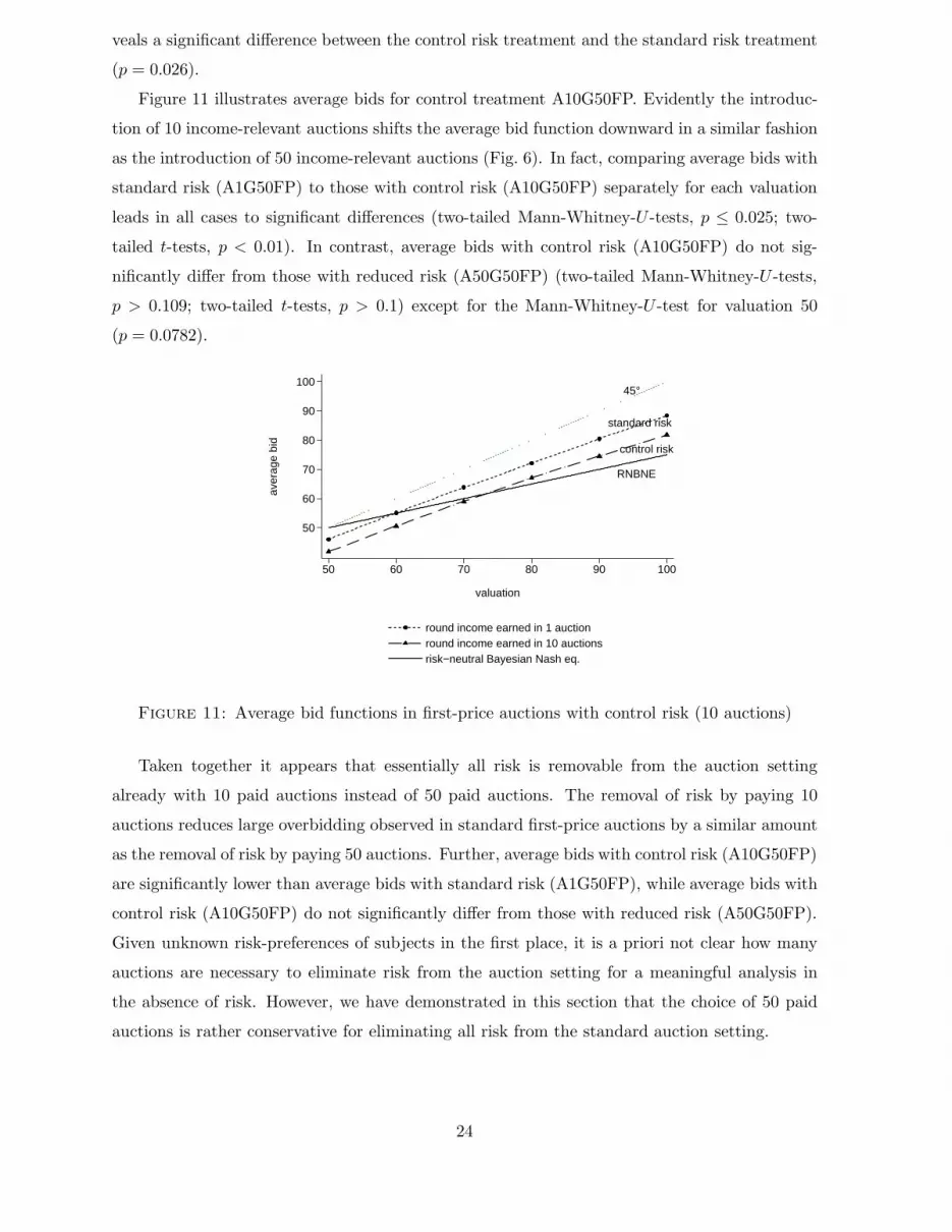
Figure 11 illustrates average bids for control treatment A10G50FP. Evidently the introduc-

tion of 10 income-relevant auctions shifts the average bid function downward in a similar fashion

as the introduction of 50 income-relevant auctions (Fig. 6). In fact, comparing average bids with

standard risk (A1G50FP) to those with control risk (A10G50FP) separately for each valuation

leads in all cases to significant differences (two-tailed Mann-Whitney-U -tests, p ≤ 0.025; two-

tailed t-tests, p < 0.01). In contrast, average bids with control risk (A10G50FP) do not sig-

nificantly differ from those with reduced risk (A50G50FP) (two-tailed Mann-Whitney-U -tests,

p > 0.109; two-tailed t-tests, p > 0.1) except for the Mann-Whitney-U -test for valuation 50

(p = 0.0782).

45°

control risk

RNBNE

standard risk

50

60

70

80

90

100

aver

age

bid

50 60 70 80 90 100

valuation

round income earned in 1 auctionround income earned in 10 auctionsrisk−neutral Bayesian Nash eq.

Figure 11: Average bid functions in first-price auctions with control risk (10 auctions)

Taken together it appears that essentially all risk is removable from the auction setting

already with 10 paid auctions instead of 50 paid auctions. The removal of risk by paying 10

auctions reduces large overbidding observed in standard first-price auctions by a similar amount

as the removal of risk by paying 50 auctions. Further, average bids with control risk (A10G50FP)

are significantly lower than average bids with standard risk (A1G50FP), while average bids with

control risk (A10G50FP) do not significantly differ from those with reduced risk (A50G50FP).

Given unknown risk-preferences of subjects in the first place, it is a priori not clear how many

auctions are necessary to eliminate risk from the auction setting for a meaningful analysis in

the absence of risk. However, we have demonstrated in this section that the choice of 50 paid

auctions is rather conservative for eliminating all risk from the standard auction setting.

24

5 Conclusion

In this paper we set out to better understand the relation between risk and bidding behavior

in auctions. Our goal goes beyond establishing that risk preferences do or do not play a role

in bidding. We are interested in assessing the relative importance of risk-preferences compared

to other phenomena that may be affecting bidders’ behavior. To this end, we introduce a novel

experimental design that not only allows us to control and gradually modify the amount of risk

that bidders experience in auctions, but also allows us to quantify to which extend deviations

from risk-neutral equilibrium bidding are due to risk aversion.

In section 4.1 we show that reducing risk, indeed, reduces the distance between the observed

and the risk-neutral equilibrium bid functions. This finding supports the hypothesis that over-

bidding in first-price auctions is at least partially due to risk-aversion. Overall, risk-aversion

explains roughly half the amount of overbidding relative to risk-neutral equilibrium in our first-

price auction setting.

Our procedure for risk-reduction is validated by the fact that reducing risk does not affect

bidding behavior in second-price auctions, in which risk-preferences theoretical should not inter-

fere with the weakly dominant equilibrium strategy. Finally, we test for the effect of increased

feedback and show that feedback has almost no effect on bidding behavior in first-price auctions

and has only a minor effect on bidding behavior in second-price auctions.

25

Appendix

A Robustness of experimental findings

In this appendix we evaluate the robustness of our findings in two ways. Firstly, we analyze

if bidding behavior changes over time, i.e. with experience, and if our findings are robust to

behavioral dynamics. Secondly, we investigate if there is heterogeneity in bidding behavior and

if individual behavior qualitatively mirrors our aggregate findings.

A.1 Stability of bidding behavior over time

Recent papers on first-price auction experiments report substantial fluctuations of bidding be-

havior in the beginning periods of first-price auction experiments decreasing over time, see

Goeree, Holt, and Palfrey (2002) and Guth et al. (2003). These behavioral dynamics might be

due to learning about the rather complex auction setting in early auction periods. Similarly,

we find much more intense fluctuations of individual bidding behavior from one period to the

next at the beginning of our experiments in all treatments. To quantify the change of submitted

bid functions from one round to the next, we measure the distance between average bid func-

0

100

200

300

2 4 6 8 10 12 2 4 6 8 10 12

first−price second−price

A1G1FP

A1G50FP

A50G50FP

A1G1SP

A1G50SP

A50G50SP

dist

ance

to p

revi

ous

bid

func

tion

period

0

.2

.4

.6

.8

1

2 4 6 8 10 12 2 4 6 8 10 12

first−price second−price

A1G1FP

A1G50FP

A50G50FP

A1G1SP

A1G50SP

A50G50SP

shar

e of

bid

ders

with

are

a<75

period

Figure 12: Evolution of bidding activity

26

tions. The distance between average bid functions is given as the area between both functions,

A(bt, bt−1). The left part of Figure 12 depicts time paths of the distance between the average

bid function submitted in period t and the average bid function that was submitted one period

earlier, in period t − 1. In the first-price treatments, the average change of bid functions from

the first period to the second period is roughly between 250 and 350 ECU. By round eight,

the average change rapidly decreased to values between roughly 50 and 75 ECU depending on

treatment and period. The evolution of the magnitude of changed bid functions is similar in

second-price auctions. Hence, there are a lot of fluctuations in the first few periods that rapidly

settle down towards the end of the experiment.

To see if the entire distribution of bidders experiences substantial fluctuations of bidding

behavior or if it is rather driven by a minority of bidders, we study the behavior of the share of

bidders with small fluctuations of bid functions over time. We consider the change of submitted

bid functions from one period to the next as small if the distance measure does not exceed 75

ECU.12 The right part of Figure 12 indicates the evolution of the share of bidders with small

fluctuations over time in any treatment. Only 30-50% of bidders modestly change their bid

functions in the first three periods of the experiment. This number grows over time. Towards

the end of the experiment the large majority of bidders, 80-90%, does not create large fluctuations

of bid functions.

Overall bidding behavior is much more stable in the second half of the experiment. To

investigate if our results reported on the behavioral effects of risk manipulation and extensive

feedback are robust to controlling for very intense fluctuations of bidding behavior, we restrict

our dataset by excluding data from periods at the beginning of the experiment. In particular we

repeat the analysis for data only from the second half of the experiment and another time for data

restricted to the last three periods. Restricting datasets in this manner does not qualitatively

affect our reported findings. Typically the p-values for the statistical tests with the restricted

datasets are smaller when we reported significant differences with the unrestricted data set. We

conclude that our findings are robust to changes of bidding behavior over time.

A.2 Individual bidding behavior

Another interesting question is if our aggregate findings on the effects of risk and feedback

variations hold on the individual level in general. Firstly, consider the risk effect with first-price

auctions. To see if individual bids are generally smaller with reduced risk than with standard

risk in the first-price auction, we compute the area below any individual bid function under

either risk treatment where individual bids are averaged over all rounds. If the computed area

measure is smaller, the underlying individual bid function is closer to the horizontal axis. Thus,

12A parallel shift of the bid function by 1.5 ECU leads to a distance of 75 ECU.

27

standard risk(A1G50FP)

reduced risk(A50G50FP)

0D

ensi

ty e

stim

ate

2500 3000 3500 4000

Area below individual bidding functions



single feedback(A1G1FP)

extensivefeedback

(A1G50FP)

0D

ensi

ty e

stim

ate

0 200 400 600 800

Absolute deviation from RNBNE (area)

feedback: 1 auction


Figure 13: Estimated density function of individual effects in first price auctions

a downward movement of individual bid functions can be seen in decreasing values of the area

measure. To geometrically represent the obtained empirical distributions of area measures, we

estimate kernel densities. The left panel of Figure 13 depicts the estimated density functions

obtained for the first-price auction. Evidently, the entire distribution appears to shift to the

left as risk is reduced so that individuals exhibit smaller area measures with reduced risk. This

reflects that the decrease of bids with reduced risk that we reported for the average bidder holds

on the individual level, too.

Secondly, consider the feedback effect under first-price auctions where extensive feedback

slightly reduces deviations from risk-neutral Bayesian Nash equilibrium. Here, we use the area

between individual bid function and the equilibrium bid function to explore effects on individual

bidding. As can be seen from the right panel of Figure 13, the density function with extensive

feedback exhibits more mass for low deviations from equilibrium in the range of 0 to 300 ECU

as compared to the density function with single feedback with more mass for medium deviations

in the range of 300 to 600 ECU. It appears that small and medium deviations decrease with

extensive feedback.

Under the assumption of independent individual average bid functions, we can use the

Kolmogorov-Smirnov test to check for significant differences of distributions. For the first-price

auction, the distribution of the area below individual bid functions with standard risk signifi-

cantly differs from that with reduced risk (p = 0.000). In contrast the distribution of equilibrium

deviations with single feedback does not significantly differ from that with extensive feedback

(p = 0.146).

For second-price auctions, we identified neither an effect of manipulations of risk nor feedback

on the average level of bid functions. As the left panel of Figure 14 suggests, the entire distri-

28

standard risk(A1G50SP)

reduced risk(A50G50SP)

0D

ensi

ty e

stim

ate

2000 3000 4000 5000 6000

Area below individual bidding functions



single feedback(A1G1SP)

extensivefeedback

(A1G50SP)

0D

ensi

ty e

stim

ate

0 1000 2000 3000

Absolute deviation from dominant strategy (area)

feedback: 1 auction


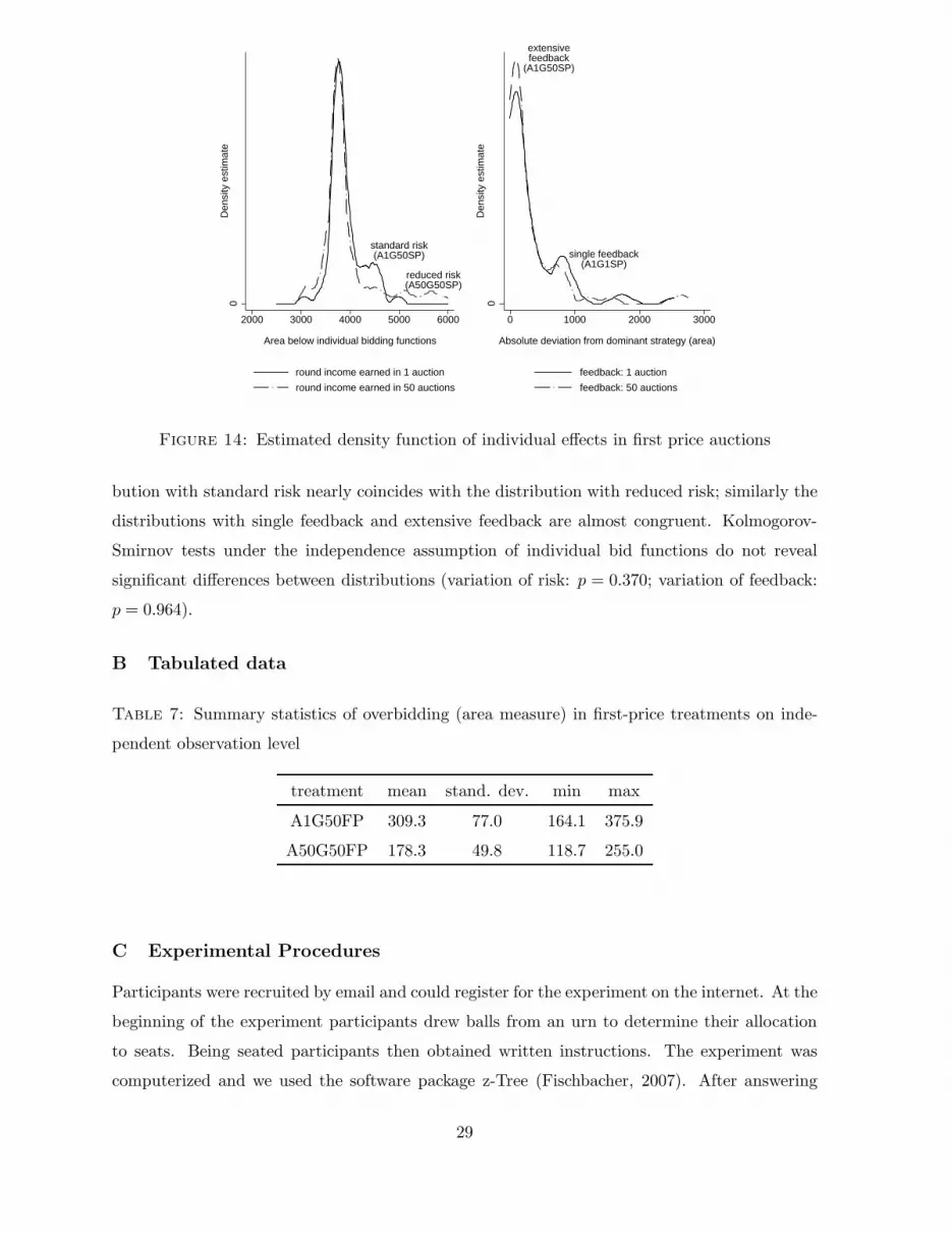
Figure 14: Estimated density function of individual effects in first price auctions

bution with standard risk nearly coincides with the distribution with reduced risk; similarly the

distributions with single feedback and extensive feedback are almost congruent. Kolmogorov-

Smirnov tests under the independence assumption of individual bid functions do not reveal

significant differences between distributions (variation of risk: p = 0.370; variation of feedback:

p = 0.964).

B Tabulated data

Table 7: Summary statistics of overbidding (area measure) in first-price treatments on inde-

pendent observation level

treatment mean stand. dev. min max

A1G50FP 309.3 77.0 164.1 375.9

A50G50FP 178.3 49.8 118.7 255.0

C Experimental Procedures

Participants were recruited by email and could register for the experiment on the internet. At the

beginning of the experiment participants drew balls from an urn to determine their allocation

to seats. Being seated participants then obtained written instructions. The experiment was

computerized and we used the software package z-Tree (Fischbacher, 2007). After answering

29

control questions on the screen participants entered the treatment described in the instructions.

After completing the treatment they answered a short questionnaire on the screen and were paid

in cash.

D Instructions

Below we provide instructions for our first-price treatments. Instruction of our second-price

treatments where similar. We used identical instructions in treatments A1G50FP, A10G50FP,

and A50G50FP. The instructions for A1G1FP were modified slightly to account for the fact that

there is feedback on a single auction as opposed to 50 auctions. The instructions are in German.

In the following we provide a translation.

D.1 General information

You are participating in a scientific experiment that is sponsored by the state Saxony-Anhalt.

If you read the following instructions carefully then you can depending on your decision gain

a considerable amount of money. It is, hence, very important that you read the instructions

carefully.

The instructions that you have received are only for your private information. During the

experiment no communication is permitted. Whenever you have questions, please raise

your hand. We will then answer your question at your seat. Not following this rule leads to

exclusion from the the experiment and all payments.

During the experiment we are not talking about Euro, but about ECU (Experimental Cur-

rency Unit). Your entire income will first be determined in ECU. The total amount of ECU that

you have obtained during the experiment will be converted into Euro at the end and paid to you

in cash. The conversion rate will be shown on your screen at the beginning of the experiment.

D.2 Information regarding the experiment

Today you are participating in an experiment on auctions. The experiment is divided into

separate rounds. We will conduct 12 rounds. In the following we explain what happens in each

round.

In each round you bid for an object that is being auctioned. Together with you another

participant is also bidding for the same object. Hence, in each round, there are two bidders.

In each round you will be allocated randomly to another participant for the auction. Your

co-bidder in the auction changes in every round. The bidder with the highest bid obtains the

object. If bids are the same the object is allocated randomly.

For the auctioned object you have a valuation in ECU. This valuation lies between 50 and

100 ECU and is determined randomly in each round. The range from 50 to 100 is shown to

30

you at the beginning of the experiment on the screen and is the same in each round. From

this range you obtain in each round new and random valuations for the object. The

other bidder in the auction also has a valuation for the object. The valuation that the other

bidder attributes to the object is determined by the same rules as your valuation and changes

in each round, too. All possible valuations of the other bidder are also in the interval from 50 to

100 from which also your valuations are drawn. All valuations between 50 and 100 are equally

likely. Your valuations and those of the other player are determined independently. You will be

told your valuation in each round. You will not know the valuation of the other bidder.

Experimental procedure The experimental procedure is the same in each round and is

described in the following. Each round in the experiment has two stages.

1st Stage

In the first stage of the experiment you see the following input screen:

- screenshot of input mode; omitted here -

At that stage you do not know your own valuation for the object in this round. On

the right side of the screen you are asked to enter a bid for six hypothetical valuations that

you might have for the object. These six hypothetical valuations are 50, 60, 70, 80, 90, and 100

ECU. Your input into this table will be shown in the graph on the left side of the screen when

you click on ”draw bids”. In the graph the hypothetical valuation is shown on the horizontal

axis, the bids are shown on the vertical axis. Your input in the table is shown as six points

in the diagram. Neighbouring points are connected with a line automatically. These

lines determine your bid for all valuations between the six points for which you have made an

input. For the other bidder the screen in the first stage looks the same. There are bids for six

hypothetical valuations, too. The other bidder can not see your input.

2nd Stage

The actual auction takes place in the second stage of each round. In each round we will

play [not in A1G1: not only] a single auction [not in A1G1: but fifty auctions]. This is done

as follows: [not in A1G1: Fifty times] a random valuation is determined that you have for the

object. Similarly for the other bidder [not in A1G1: fifty random valuations are] [in in A1G1:

one valuation is] determined. [not in A1G1: The screen lists all auctions ordered by valuations.]

You see the following screen:

- screenshot feedback13; omitted here -

For [only in A1G1: your valuation] [not in A1G1: each of the fifty valuations] the computer

determines your bid according to the graph from stage 1. If [in A1G1: your] [not in A1G1: a]

13The given screenshot for treatment A1G1 differed from that for all other treatments only in the number of

displayed auctions. Drawn valuations, bids, and incomes were always replaced by ’...’ in all instructions.

31

valuation is precisely at 50, 60, 70, 80, 90, or 100 the computer takes the bid that you gave for

this valuation. If [in A1G1: your] [not in A1G1: a] valuation is between these points your bid

is determined according to the joining line. In the same way the [in A1G1: bid ] [not in A1G1:

bids] of the other bidder [in A1G1: is ] [not in A1G1: are] determined [not in A1G1: for his fifty

valuations]. Your bid is compared with the one of the other bidder. The bidder with the higher

bid obtains the object. If you are the bidder with the higher bid, then your income from this

auction will be shown. If you are the bidder with the smaller bid, then a dot (.) will be shown

instead of the income.

Your income from the auction:

[not in A1FG: A fixed number of auctions out of all 50 auctions will be randomly selected and

marked by an asterisk (*). The outcomes of these marked auctions determine your income in

this round. All auctions that are not marked do not change your account balance. The number

of marked auctions is the same in every round and will be shown on a screen at the start of the

experiment.]

[not in A1G1: For each of the randomly selected auctions that are marked by an asterisk (*)

the] [only in A1G1: The] following holds:

• The bidder with the higher bid obtains the valuation he had for the object in this auction

added to his account minus his bid for the object.

• The bidder with the smaller bid obtains no income from this auction.

You total income in a round is [not in A1G1: the sum of ] the ECU income from the

[not in A1G1: marked auctions] [in A1G1: auction] in this round where you have made

the higher bid.

This ends one round of the experiment and you see in the next round again the input screen

from stage 1. At the end of the experiment your total ECU income from all rounds will be

converted into Euro and paid to you in cash together with your Show-Up Fee of 3.00 Euro.

Please raise your hand if you have questions.

32

References

Abbink, Klaus, Bernd Irlenbusch, Paul Pezanis-Christou, Bettina Rockenbach, and Abdolkarim

Sadrieh (2005): An experimental test of design alternatives for the British 3G/UMTS auction,

European Economic Review 49(2), 505-530.

Andreoni, James, Yeon-Koo Che, and Jinwoo Kim (2007): Asymmetric information about rival’s

types in standard auctions: An experiment, Games and Economic Behavior 59, 240-259.

Brosig, Jeannette, and J. Philipp Reiss (2007): Entry decisions and bidding behavior in se-

quential procurement auctions: An experimental study, Games and Economic Behavior 58(1),

50-74.

Chen, Kay-Yut, and Charles R. Plott (1998), Nonlinear behavior in sealed bid first-price auc-

tions, Games and Economic Behavior, 3478.

Cooper, David J. and Hanming Fang (forthcoming): Understanding Overbidding in Second

Price Auctions: An Experimental Study, Economic Journal.

Cox, James C., Vernon L. Smith, and James M. Walker (1985): Experimental Development

of Sealed-Bid Auction Theory: Calibrating Controls for Risk Aversion, American Economic

Review 75(2), 160-165.

Cox, James C., Vernon L. Smith, and James M. Walker (1988), Theory and individual behavior

of first-price auctions, Journal of Risk and Uncertainty 1, 6199.

Cramton, Peter C. (1995): Money out of thin air: The nationwide narrowband PCS auction,

Journal of Economics and Management Strategy 4, 267-343.

Crawford, Vincent P., and Nagore Iriberri (2007): Level-k Auctions: Can a Non-Equilibrium

Model of Strategic Thinking Explain the Winner’s Curse and Overbidding in Private-Value

Auctions?, Econometrica 75, 1721-1770.

Engelbrecht-Wiggans, Richard, and Elena Katok (forthcoming): Regret and Feedback Informa-

tion in First-Price Sealed-Bid Auctions, Management Science, forthcoming.

Engelbrecht-Wiggans, Richard, and Elena Katok (2007a): Regret in Auctions: Theory and

Evidence, Economic Theory 33, 81-101.

Engelbrecht-Wiggans, Richard, and Elena Katok (2007b): A Direct Test of Risk Aversion and

Regret in First Price Sealed Bid Auctions, Working Paper.

33

Filiz-Ozbay, Emel, and Erkut Y. Ozbay (2007): Auctions with Anticipated Regret: Theory and

Experiment, American Economic Review 97(4), 1407-1418.

Fischbacher, Urs (2007): z-Tree: Zurich Toolbox for Ready-made Economic Experiments, Ex-

perimental Economics 10(2), 171-178.

Garratt, Rod, Walker, Mark, and John Wooders (2004): Behavior in Second-Price Auctions by

Highly Experienced eBay Buyers and Sellers, Working Paper.

Garratt, Rod, and John Wooders (2004): Efficiency in Second-Price Auctions: A New Look at

Old Data, Working Paper.

Goeree, Jacob K., Holt, Charles A., and Thomas Palfrey (2002): Quantal response equilibrium

and overbidding in private-value auctions. Journal of Economic Theory 104, 247272.

Guth, Werner, Radosveta Ivanova-Stenzel, Manfred Konigstein, and Martin Strobel (2002): Bid

functions in auctions and fair division games: experimental evidence. German Economic Review

3(4), 461-484.

Guth, Werner, Radosveta Ivanova-Stenzel, Manfred Konigstein, and Martin Strobel (2003):

Learning to bid - an experimental study of bid function adjustments in auctions and fair division

games, Economic Journal 113, 477-494.

Harstad, Ron (2000): Dominant strategy adoption and bidders’ experience with pricing rules,

Experimental Economics 3, 261-280.

Isaac, R. Mark, and James M. Walker (1985): Information and Conspiracy in Sealed Bid Auc-

tions, Journal of Economic Behavior and Organization 6, 139-159.

Holt, Charles A. and Susan K. Laury (2002): Risk Aversion and Incentive Effects, American

Economic Review 92(3), 1644-1655.

Kagel, John H. (1995): Auctions: a survey, in: Kagel, John H. und Alvin E. Roth (eds.),

Handbook of Experimental Economics. Princeton: Princeton University Press, 501-585.

Kagel, John H. and Dan Levin (1993): Independent private values auctions: Bidder behavior

in first-, second-, and third-price auctions with varying numbers of bidders, Economic Journal

103, 868-879.

Kagel, John H., Harstad, Ron, and Dan Levin (1987): Information impact and allocation rules

in auctions with affliated private values: a laboratory study, Econometrica 55(6), 1275-1304.

Kirchkamp, Oliver, Poen, Eva, and J. Philipp Reiss (forthcoming): Outside Options: Another

reason to choose the first-price auction, European Economic Review.

34

Kirchkamp, Oliver and J. Philipp Reiss (2004): The overbidding-myth and the underbidding-bias

in first-price auctions, SFB 504 discussion paper 04-32, University of Mannheim.

Maskin, Eric, and John Riley (1984): Optimal auctions with risk averse buyers, Econometrica 52,

1473-1518.

Matthews, Steven A. (1987): Comparing auctions for risk averse buyers: A buyer’s point of

view, Econometrica 55(3), 633-646.

McMillan, John (1994): Selling Spectrum Rights, Journal of Economic Perspectives 8(3), 145-

162.

Milgrom, Paul (2004): Putting auction theory to work”, Cambridge University Press.

Morgan, John, Steiglitz, Kenneth, and George Reis (2003): The spite motive and equilibrium

behavior in auctions, Contributions to Economic Analysis & Policy, 2(1), article 5.

Neugebauer, Tibor, and Reinhard Selten (2006): Individual behavior in first-price auctions:

The importance of information feedback in computerized experimental markets, Games and

Economic Behavior 54, 183-204.

Ockenfels, Axel and Reinhard Selten (2005): Impulse Balance Equilibrium and Feedback in First

Price Auctions, Games and Economic Behavior 51, 155–170.

Pezanis-Christou, Paul and Abdolkarim Sadrieh (2004): Elicited bid functions in (a)symmetric

first-price auctions, Working Paper.

Rogers, W. H., 1993. Regression standard errors in clustered samples. Stata Technical Bulletin

13, 19–23. Reprinted in Stata Technical Bulletin Reprints 3, 88–94.

Roth, Alvin E., and Michael W.K. Malouf (1979), Game-theoretic models and the role of infor-

mation in bargaining, Psychological Review 86, 574594.

Selten, Reinhard, and Joachim Buchta (1999): Experimental sealed bid first price auctions with

directly observed bid functions. In: (Budescu, D., Erev, I., Zwick, R., eds.) Games and Human

Behavior: Essays in the Honor of Amnon Rapoport, Mahwah, NJ: Lawrenz Associates, 79102.

Selten, Reinhard, Abdolkarim Sadrieh, and Klaus Abbink (1999): Money does not induce risk

neutral behavior, but binary lotteries do even worse, Theory and Decision 46(3), 213-252.

Smith, Vernon L. and James M. Walker (1993): Rewards, Experience and Decision Costs in

First Price Auctions, Economic Inquiry 31, 237-245.

35

Vogt, Carsten, Weimann, Joachim, and Chun-Lei Yang (2002): Efficient Rent-Seeking in Ex-

periment, Public Choice 110(1-2), 67-78.

36

Documents

A pure variation of risk in …rst-price auctions