A rational approach to design of vertical drains considering soil disturbance

A Rational Approach to the Design of Vertical Drains Considering Soil Disturbance

Dipanjan Basu1, C. Eng., M. ASCE, Prasenjit Basu2, A.M. ASCE

and Monica Prezzi3, A.M. ASCE

1Assistant Professor, Department of Civil and Environmental Engineering, University of Waterloo, 200 University Avenue W, Waterloo, ON N2L 3G1, Canada, E-mail: [email protected]

2Assistant Professor, Department of Civil and Environmental Engineering, Pennsylvania State University, 213C Sackett Building, University Park, PA 16802, E-mail: [email protected]

3Professor, School of Civil Engineering, Purdue University, 550 Stadium Mall Drive, West Lafayette, IN 47907, E-mail: [email protected]

ABSTRACT This paper presents analytical solutions for the rate of consolidation by prefabricated vertical drains (PVDs) that take into account the properties of soft, clayey soils, the disturbance in the soil surrounding the PVD caused by the installation process, and PVD dimension and spacing. A particular feature of the analysis is that it rigorously takes into account the spatial variability of the soil hydraulic conductivity of the disturbed soil mass around the PVD. Design charts are developed based on the analytical solutions that can be used to determine PVD spacing without requiring any iteration. A numerical example is provided that illustrates the design procedure. INTRODUCTION

Thick alluvial deposits of soft clayey soil are characterized by low shear strength, high compressibility and low hydraulic conductivity. Pre-treatment of these deposits by the installation of prefabricated vertical drains (PVDs), often in conjunction with preloading, is a popular practice in geotechnical engineering. The installation of PVDs generates hydraulic gradients that drive the pore water out of the deposit through the PVDs and into a drainage blanket. Because PVDs are installed with a close horizontal spacing of about 1 to 3 m, the drainage path inside the soil is greatly reduced and consolidation of the soil deposit is accelerated (Holtz 1987).

There are some operational problems associated with PVDs. One such problem arises from the disturbance caused to the ground during installation of the PVDs. Due to this disturbance, the hydraulic conductivity of the soil surrounding the PVD decreases significantly from the in situ value, slowing down the consolidation process. Therefore, the effect of soil disturbance must be taken into account in PVD

551

Sound Geotechnical Research to Practice

Dow

nloa

ded

from

asc

elib

rary

.org

by

Uni

vers

ity o

f W

ater

loo

on 0

8/03

/15.

Cop

yrig

ht A

SCE

. For

per

sona

l use

onl

y; a

ll ri

ghts

res

erve

d.

design. Studies on soil disturbance have mostly considered a constant reduced hydraulic conductivity in the disturbed soil (Hansbo 1981, Indraratna and Redana 1997). However, recent studies (Onoue et al. 1991, Madhav et al. 1993, Indraratna and Redana 1998, Sharma and Xiao 2000) show that the hydraulic conductivity varies spatially within the disturbed mass of soil surrounding the PVD and that considering this spatial variation is important for the analysis and design of PVDs (Basu et al. 2006, Basu and Prezzi 2007, 2009).

Robert D. Holtz devoted part of his career studying the behavior of PVDs (Holtz and Holm 1973, Holtz 1987) in fact he was one of the pioneers who suggested that the soil hydraulic conductivity varies spatially in the disturbed soil (Holtz et al. 1991). In this paper, analytical solutions considering the spatial variation of the disturbed hydraulic conductivity are presented. First, the hydraulic conductivity within the disturbed soil zone is characterized based on laboratory and field test data. Using the characterized hydraulic conductivity profiles, closed-form solutions are developed. Subsequently, a design methodology is outlined that can be use to determine PVD spacing without any iteration. Design charts are prepared using the developed analytical solutions to aid the design process. HYDRAULIC CONDUCTIVITY IN THE DISTURBED ZONE

The spatial variation of the hydraulic conductivity khd for horizontal flow in the disturbed zone of soil surrounding a PVD can be approximated by a sigmoidal curve (Fig. 1). A sigmoidal curve matches the experimentally observed profiles obtained by Onoue et al. (1991), Madhav et al. (1993), Indraratna and Redana (1998) and Sharma and Xiao (2000), and can be expressed as

,1 1 m eq

r

rhd hs hs

ho ho ho

k k ke

k k k

(1)

where khs is the hydraulic conductivity for horizontal flow in the region immediately adjacent to the PVD; kho is the in situ undisturbed horizontal hydraulic conductivity; r is the radial distance from the PVD center (with the assumption that the PVD and the disturbed zone are circular in plan), rm,eq is the equivalent mandrel radius (obtained by equating the actual mandrel cross sectional area to a circular area); and and are fitting parameters. Hydraulic conductivity profiles with = 0.45 to 2.0 and = 30 and with khs/kho = 0.1, 0.2 and 0.3 were found to cover the range of experimentally observed spatial variation of the hydraulic conductivity (Fig. 1).

The size and shape of the disturbed zone surrounding the PVD is not known with certainty. According to Fig. 1, the location of the outer boundary of the disturbed zone (as measured from the center of the drain) can vary from 4 to 18 times the equivalent mandrel radius. The shape of the disturbed zone is most likely governed by the shape of the mandrel used to install the PVD. If a square or circular mandrel is used for PVD installation, the disturbed zone shape is likely to be a square or a circle

SOUND GEOTECHNICAL RESEARCH TO PRACTICE: HONORING ROBERT D. HOLTZ II552


Dow

nloa

ded

from

asc

elib

rary

.org

by

Uni

vers

ity o

f W

ater

loo

on 0

8/03

/15.

Cop

yrig

ht A

SCE

. For

per

sona

l use

onl

y; a

ll ri

ghts

res

erve

d.

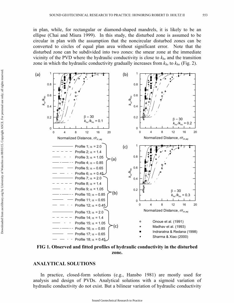
in plan, while, for rectangular or diamond-shaped mandrels, it is likely to be an ellipse (Chai and Miura 1999). In this study, the disturbed zone is assumed to be circular in plan with the assumption that the noncircular disturbed zones can be converted to circles of equal plan area without significant error. Note that the disturbed zone can be subdivided into two zones: the smear zone at the immediate vicinity of the PVD where the hydraulic conductivity is close to khs and the transition zone in which the hydraulic conductivity gradually increases from khs to kho (Fig. 2).

Profile 1; = 2.0

Profile 2; = 1.4

Profile 3; = 1.05

Profile 4; 0.85

Profile 5; 0.65

Profile 6; = 0.45

(a)

(b)

Profile 7; = 2.0

Profile 8; = 1.4

Profile 9; = 1.05

Profile 10; 0.85

Profile 11; 0.65

Profile 12; = 0.45

(c)

Profile 13; = 2.0

Profile 14; = 1.4

Profile 15; = 1.05

Profile 16; 0.85

Profile 17; 0.65

Profile 18; = 0.45

0 4 8 12 16 20

Normalized Distance, r/rm,eq

0

0.2

0.4

0.6

0.8

1

k hd /k

ho

30khs /kho = 0.2

Onoue et al. (1991)

Madhav et al. (1993)

Indraratna & Redana (1998)

Sharma & Xiao (2000)

(a) (b)

(c)

0 4 8 12 16 20


0

0.2

0.4

0.6

0.8

1

k hd /k

ho

30khs /kho = 0.1

0 4 8 12 16 20


0

0.2

0.4

0.6

0.8

1

k hd /k

ho

30khs /kho = 0.3

FIG 1. Observed and fitted profiles of hydraulic conductivity in the disturbed

zone.

ANALYTICAL SOLUTIONS

In practice, closed-form solutions (e.g., Hansbo 1981) are mostly used for analysis and design of PVDs. Analytical solutions with a sigmoid variation of hydraulic conductivity do not exist. But a bilinear variation of hydraulic conductivity

SOUND GEOTECHNICAL RESEARCH TO PRACTICE: HONORING ROBERT D. HOLTZ II 553


Dow

nloa

ded

from

asc

elib

rary

.org

by

Uni

vers

ity o

f W

ater

loo

on 0

8/03

/15.

Cop

yrig

ht A

SCE

. For

per

sona

l use

onl

y; a

ll ri

ghts

res

erve

d.

in the transition zone with constant hydraulic conductivity in the smear zone closely follows the sigmoid variation (Fig. 2). Such a variation is used to develop analytical solutions in this study. It is assumed that PVDs are installed in a homogeneous deposit of saturated soft clay. A typical PVD is considered in the analysis, and the drain and its zone of influence, known as the unit cell, are assumed to be circular in plan with radii rd and rc, respectively. The disturbed zone is divided into two distinct parts: a smear zone with a radius rs and a transition zone with an outer radius rt. The hydraulic conductivity is spatially constant at khs in the smear zone and it increases in the transition zone linearly to khp at a radial distance rp (measured from the center of the drain) following one slope and then to kho at the outer boundary of the disturbed zone following another slope. It is assumed that the length of the drain spans the entire thickness of the soil deposit and that vertical flow in the soil is negligible. Equal strain consolidation of the unit cell with spatially uniform vertical strain and no horizontal strain is also assumed. The axisymmetric horizontal flow of water from the unit cell into the drain is assumed to follow Darcy’s law.

(a) (b) FIG 2. Schematic showing assumed analytical geometry: (a) unit cell with disturbed zone, and (b) associated distribution of hydraulic conductivity.

A radial coordinate r with its origin at the center of the drain is assumed. The domain rd r rc is divided into four zones: the smear zone with rd r rs, the inner transition zone with rs r rp (in which khd increases from khs to khp), the outer transition zone with rp r rt (in which khd increases from khp to kho) and the remaining annular area outside the transition zone with rt r rc. Within any zone Z, the specific discharge is given by

Z ZZ

w

k uv

r

(2)

Circular Undisturbed

Zone

rc

rs

Circular Unit Cell

Circular Drain

rt

Circular Transition

Zone

Circular Smear Zone

Undisturbed Zone

0

Bilinear Variation for Analytical Solution

r/rm,eq

khd /kho

1.0

0

Sigmoid Variation

Transition Zone

SmearZone

hss

ho

k

k

hpp

ho

k

k

,

t

m eq

r

r,

p

m eq

r

r,

s

m eq

r

r



Dow

nloa

ded

from

asc

elib

rary

.org

by

Uni

vers

ity o

f W

ater

loo

on 0

8/03

/15.

Cop

yrig

ht A

SCE

. For

per

sona

l use

onl

y; a

ll ri

ghts

res

erve

d.

where the subscript Z is used to denote any of the above four zones with a hydraulic conductivity kZ and excess pore pressure uZ. The variation of hydraulic conductivity in the inner and outer transition zones are given by

1( ) hs p hp s hp hshd

p s p s

k r k r k kk r r

r r r r

; (rs r rp) (3)

2 ( ) hp t ho p ho hphd

t p t p

k r k r k kk r r

r r r r

; (rp r rc) (4)

Considering a cylinder of an arbitrary radius r (r < rc) within the unit cell, the total

volume of water entering into the cylinder (of radius r) from the outer hollow cylinder (of thickness rc – r) must be equal to the change in volume of the outer hollow cylinder. Using this concept, the specific discharge within the unit cell can be related to the vertical strain v as

2 22 vZ crv r r

t

(5)

where t is the time. The above equation is valid for any zone Z. Replacing vZ in the above equation by equation (2) produces the relationship between the spatial variation of excess pore pressure and the temporal variation of the vertical strain

2

2Z w c v

Z

u rr

r k r t

(6)

The summation of the integrals of excess pore pressure uZ over the corresponding domain Z divided by the total area of the unit cell gives the average excess pore pressure ū throughout the unit cell as

1 2

2 2

2 2 2 2ps t c

d s p t

rr r r

s t t c

r r r r

c d

ru dr ru dr ru dr ru dr

ur r

(7)

where us, ut1, ut2 and uc are the excess pore pressures in the smear, inner transition, outer transition and undisturbed zones, respectively. Integrating Eq. (6) with respect to r for each of the zones Z with the boundary conditions us = 0 at r = rd, us = ut1 at r = rs, ut1 = ut2 at r = rp, ut2 = uc at r = rt and substituting in Eq. (7), the following equation is obtained



Dow

nloa

ded

from

asc

elib

rary

.org

by

Uni

vers

ity o

f W

ater

loo

on 0

8/03

/15.

Cop

yrig

ht A

SCE

. For

per

sona

l use

onl

y; a

ll ri

ghts

res

erve

d.

2

2w c v

ho

ru

k t

(8)

where is given by

1 3ln ln ln ln

4ps

s ps p p

qp m q ppnm

q m pp m q p

(9)

after neglecting the terms that contributed to a difference of less than 3% in the values of . The parameters in Eq. (9) are defined as n = rc/rd, m = rs/rd, q = rt/rd, p = rp/rd, s = khs/kho and p = khp/kho.

Assuming that all the excess pore pressure due to preloading is developed instantly at t = 0, the following relationship can be written

vv v

um m

t t t

(10)

where is the average effective stress in the unit cell, ū is the average excess pore pressure, and mv is the coefficient of volume compressibility. Substituting Eq. (8) into Eq. (10) to eliminate v t , the following linear differential equation is obtained

2

20c

v w c

du ku

dt m r (11)

Solving Eq. (11) using the initial condition 0u u at t = 0, in which 0u is the initial

average excess pore pressure at the time of load application, and replacing t with the

time factor 24h cT c t r , in which ch is the coefficient of consolidation for

horizontal flow given by h ho v wc k m , the following equation is obtained

8

0

T

u u e

(12)

The degree of consolidation U at any time t (or time factor T) is the ratio of the excess pore pressure dissipated to the initial excess pore pressure. U is mathematically expressed as 01U u u , which along with Eq. (12) gives

81 TU e (13)



Dow

nloa

ded

from

asc

elib

rary

.org

by

Uni

vers

ity o

f W

ater

loo

on 0

8/03

/15.

Cop

yrig

ht A

SCE

. For

per

sona

l use

onl

y; a

ll ri

ghts

res

erve

d.

Overlapping of Disturbed Zones

The disturbed zones surrounding the PVDs may extend beyond the unit cell and interfere with the adjacent unit cells. This leads to overlap of disturbed zones of adjacent unit cells and such overlap must be taken into account. In order to generate analytical solutions, it is assumed that the actual zones of overlap can be replaced by axisymmetric overlap zones, as was done by Walker and Indraratna (2007). It is also assumed that the gradual increase of the hydraulic conductivity with increasing radial distance from the PVD occurs only up to the point (denoted by L in Fig. 3) where the overlap of the disturbed zones begins (i.e., up to r = rl in Fig. 3). Beyond r = rl (i.e., within the overlap zone), the hydraulic conductivity remains constant at khl (< kho), which is equal to the corresponding value of the hydraulic conductivity at the boundary of the disturbed zone and the overlap zone. Such an assumption gives rise to three possibilities (Fig. 3). If the zone of overlap is limited in extent (i.e., if rl > rp), then the modified (overlapped) hydraulic conductivity profile may be approximated by the bilinear variation of hydraulic conductivity in the transition zone, similar to that shown in Fig. 2(b) (Case A). If the zone of overlap increases (i.e., if rs < rl < rp), then the bilinear variation does not properly match the overlapped hydraulic conductivity profile, and a linear variation of hydraulic conductivity in the transition zone has to be assumed (Case B). It is possible (although not desirable) that the overlap zone is very large (i.e., rl < rs), in which case the entire unit cell may be assumed to have a constant hydraulic conductivity equal to that within the smear zone (Case C).

Mathematically, the modified (overlapped) hydraulic conductivity profiles can be defined by the ratios l dl r r and l hl hok k in which rl is the distance from the

center of the drain to the point at which the zone of overlap starts and khl is the constant hydraulic conductivity in the overlap zone. These parameters l andl are related to the parameters m, p, q, p and s as

2l n q (14)

1 (Case A)

(Case B)

(Case C)

p p

l p s s

s

l p

q p

l m

p m

(15)

For Case A, the analytical solution described above is valid after modifications.

For Case B, a similar analytical solution is developed (Basu et al. 2006) and, for Case C, the analytical solution by Barron (1948) can be used after modifications. Thus, Eq. (13) can be used to describe U versus T relationships for all the cases A, B and C with given by:



Dow

nloa

ded

from

asc

elib

rary

.org

by

Uni

vers

ity o

f W

ater

loo

on 0

8/03

/15.

Cop

yrig

ht A

SCE

. For

per

sona

l use

onl

y; a

ll ri

ghts

res

erve

d.

FIG 3. Overlap of disturbed zones: (a) axisymmetric overlap zone, and modified

hydraulic conductivity profiles for (b) Case A, (c) Case B, and (d) Case C.

1 3ln ln ln ln

4

1 3ln ln ln

4

1 3ln

4

pl ll s

l s p ls p p l

ll s

l s s l l

s

lp m l ppnm

l m pp m l p

l m lnm

l l m m

n

(16)

rc

Unit Cell

Drain

rl

Circular Overlap Zone

rs

Smear Zone

khs

kho

Smear TransitionOverlapkhd khd

L

,

l

m eq

r

r ,

s

m eq

r

r ,

c

m eq

r

r ,

t

m eq

r

r

kho

khp

SmearTransition

Overlap

khs

khd khd

L

khl

,

s

m eq

r

r ,

l

m eq

r

r,

p

m eq

r

r,

c

m eq

r

r ,

t

m eq

r

r

kho

khp

khl

SmearTransition

Overlap

khs

khd khd

L

,

s

m eq

r

r ,

p

m eq

r

r,

l

m eq

r

r ,

c

m eq

r

r ,

t

m eq

r

r

(a) (b)

(c) (d)



Dow

nloa

ded

from

asc

elib

rary

.org

by

Uni

vers

ity o

f W

ater

loo

on 0

8/03

/15.

Cop

yrig

ht A

SCE

. For

per

sona

l use

onl

y; a

ll ri

ghts

res

erve

d.

in which the first equation is valid for Case A, the second equation is valid for Case B and the third equation is valid for Case C. DESIGN METHODOLOGY AND CHARTS

Design of PVDs generally involves the calculation of the horizontal spacing of PVD installation. For calculating the PVD spacing, an initial guess for the spacing (which determines n in Eq. (9) or (16)) has to be made first, based on which the time factor corresponding to the desired degree of consolidation is calculated. Consequently, iterations are required to determine the PVD spacing corresponding to the desired degree of consolidation within a certain time. Yeung (1997) developed a method by which this iteration procedure can be avoided. The method of Yeung (1997) is adopted here, and, as outlined below, applied to the developed analytical solution. A modified time factor T' is defined as

24h

d

c tT

r (17)

Using Eq. (17), the degree of consolidation U in Eq. (13) can be rewritten as

8

1T

U e

(18)

where

2n (19) In the above equation for , can be obtained from Eq. (9) or (16). Defining a new normalized time factor T as T T (20) a unique relationship between T and U can be obtained as

ln 1

8

UT

(21)

Equation (19) is used to develop plots relating n and ' for the different hydraulic

conductivity profiles shown in Fig. 1. In order to develop these plots, three equivalent mandrel radius rm,eq = 46.0 mm, 68.7 mm and 84.6 mm are considered that are representatives of the dimensions of the mandrels used in practice. The PVD spacing s is assumed to range between 0.9 to 3.5 m, which produces an equivalent unit cell radius rc,eq in the range of 0.47 to 1.84 m for triangular arrangement (for



Dow

nloa

ded

from

asc

elib

rary

.org

by

Uni

vers

ity o

f W

ater

loo

on 0

8/03

/15.

Cop

yrig

ht A

SCE

. For

per

sona

l use

onl

y; a

ll ri

ghts

res

erve

d.

which rc,eq = 0.525s) and in the range of 0.51 to 1.98 m for square arrangement (for which rc,eq = 0.564s). The equivalent unit cell radius is obtained by equating the area of the actual hexagonal or square unit cell to that of an equivalent circle. A PVD cross-sectional dimension of 100 mm 4 mm is assumed for the generation of these plots, which produced an equivalent drain radius rd,eq = 33.1 mm (obtained by equating the perimeter of the PVD with the perimeter of an equivalent circle with radius rd,eq). This produces an equivalent parameter n (= rc,eq/rd,eq) in the range of 15 to 60.

Based on the above values, the possible range of values for m, p, q, s and p (i.e., parameters related to the degree of disturbance and to the extent of the disturbed zone) are calculated for the range of possible hydraulic conductivity profiles shown in Fig. 1 and for the chosen mandrel radii. This is done by matching the sigmoid variation of the hydraulic conductivity profiles given in Fig. 1 with the bilinear variation described in Fig. 2(b). Tables 1 and 2 show the values of the different parameters obtained after matching the sigmoid curves with the corresponding bilinear curves. The values given in Tables 1 and 2 are used to estimate .

Using the values of the parameters given in Tables 1 and 2, ' versus n charts are generated, as shown in Figs. 4 through 6, for the hydraulic conductivity profiles in Fig. 1. In these calculations, the possibility of overlap of the disturbed zones is taken into account for cases with q > n. If overlap occurs (i.e., if q > n), then the particular case of overlap (out of Cases A, B and C) is identified based on one of the three prevailing conditions, l > p, m < l < p and l < m, and Eqs. (15) and (16) are accordingly used in the calculations. The plots in Figs. 4 through 6 include the cases where overlap occurred. Site specific ' versus n curves, similar to Figs. 4 through 6, can be developed following the procedure described above if the actual hydraulic conductivity profile of the site is known.

In design, the drain geometry (i.e., rd), soil property ch, time t available (within which a certain percentage of consolidation has to be completed) and the desired degree of consolidation U are required as input. Using these data, T' and T can be calculated from Eqs. (17) and (21), respectively, from which ' can be calculated using Eq. (20). With the calculated value of ', n can be determined from the ' versus n charts (Figs. 4 through 6) from which the desired PVD spacing can be calculated without any iteration.



Dow

nloa

ded

from

asc

elib

rary

.org

by

Uni

vers

ity o

f W

ater

loo

on 0

8/03

/15.

Cop

yrig

ht A

SCE

. For

per

sona

l use

onl

y; a

ll ri

ghts

res

erve

d.

TABLE 1. Normalized radial distances related to the disturbed zone Hydraulic

Conductivity Profile

rs /rm,eq rp /rm,eq rt /rm,eq

1, 7, 13 2.0 1.2 2.6 4.2

2, 8, 14 1.4 1.5 3.9 6.2

3, 9, 15 1.05 2.1 4.9 8.2

4, 10, 16 0.85 2.7 5.7 10.0

5, 11, 17 0.65 3.5 7.7 13.0

6, 12, 18 0.45 5.0 11.2 18.0

TABLE 2. Parameters for use in Eq. (9) or Eq. (16)

† These profiles may cause overlap for rm,eq = 46.0 mm ‡ These profiles may cause overlap for rm,eq = 68.7 mm * These profiles may cause overlap for rm,eq = 84.6 mm

Profile s p rm,eq = 46.0 mm rm,eq = 68.7 mm rm,eq = 84.6 mm m p q m p q m p q

1 0.1 0.9 1.7 3.6 6.1 2.5 5.4 9.1 3.1 6.7 11.32* 0.1 0.9 2.1 5.4 8.6 3.1 8.1 12.9 3.8 10.0 15.93‡* 0.1 0.9 2.9 6.8 11.4 4.4 10.2 17.0 5.4 12.5 21.04‡* 0.1 0.9 4.0 7.9 13.9 6.0 11.8 20.1 7.4 14.6 25. 65†‡* 0.1 0.9 5.0 10.6 18.1 7.5 15.8 27.0 9.2 19.4 33.26†‡* 0.1 0.9 7.2 15.6 25.0 10.8 23.3 37.4 13.3 28.6 46.0

7 0.2 0.9 1.7 3.5 5.8 2.5 5.2 8.7 3.1 6.4 10.78* 0.2 0.9 2.1 5.4 8.6 3.1 8.1 12.9 3.8 10.0 15.99‡* 0.2 0.9 2.9 6.8 11.4 4.4 10.2 17.0 5.4 12.5 21.010‡* 0.2 0.9 3.8 7.9 13.9 5.6 11.8 20.1 6.9 14.6 25.611†‡* 0.2 0.9 4.7 10.8 18.1 7.1 16.2 27.0 8.7 19.9 33.212†‡* 0.2 0.9 7.0 15.6 25.0 10.4 23.3 37.4 12.8 28.6 46.0

13 0.3 0.9 1.7 3.6 5.8 2.5 5.4 8.7 3.1 6.7 10.714* 0.3 0.9 2.2 5.0 8.6 3.3 7.5 12.9 4.1 9.2 15.915‡* 0.3 0.9 2.9 6.8 11.4 4.4 10.2 17.0 5.4 12.5 21.016‡* 0.3 0.9 3.8 8.2 13.9 5.6 12.3 20.8 6.9 15.1 25. 617†‡* 0.3 0.9 4.9 10.7 18.1 7.3 16.0 27.0 9.0 19.7 33.218†‡* 0.3 0.9 6.8 15.7 25.0 10.1 23.5 37.4 12.5 28.9 46.0



Dow

nloa

ded

from

asc

elib

rary

.org

by

Uni

vers

ity o

f W

ater

loo

on 0

8/03

/15.

Cop

yrig

ht A

SCE

. For

per

sona

l use

onl

y; a

ll ri

ghts

res

erve

d.

1000 10000 100000

10

20

30

40

50

60

n

Profile 1

Profile 2

Profile 3

Profile 4

Profile 5

Profile 6

rm = 46.0 mmkhs /kho = 0.1

1000 10000 100000

10

20

30

40

50

60

n

Profile 7

Profile 8

Profile 9

Profile 10

Profile 11

Profile 12

rm = 46.0 mmkhs /kho = 0.2

(a) (b)

1000 10000 100000

10

20

30

40

50

60

n

Profile 13

Profile 14

Profile 15

Profile 16

Profile 17

Profile 18

rm = 46.0 mmkhs /kho = 0.3

(c)

FIG 4. ' versus n curves for mandrel radius rm = 46.0 mm



Dow

nloa

ded

from

asc

elib

rary

.org

by

Uni

vers

ity o

f W

ater

loo

on 0

8/03

/15.

Cop

yrig

ht A

SCE

. For

per

sona

l use

onl

y; a

ll ri

ghts

res

erve

d.

1000 10000 100000

10

20

30

40

50

60n

Profile 1

Profile 2

Profile 3

Profile 4

Profile 5

Profile 6

rm = 68.7 mmkhs /kho = 0.1

1000 10000 100000

10

20

30

40

50

60

nProfile 7

Profile 8

Profile 9

Profile 10

Profile 11

Profile 12

rm = 68.7 mmkhs /kho = 0.2

(a) (b)

1000 10000 100000

10

20

30

40

50

60

n

Profile 13

Profile 14

Profile 15

Profile 16

Profile 17

Profile 18

rm = 68.7 mmkhs /kho = 0.3

(c)




Dow

nloa

ded

from

asc

elib

rary

.org

by

Uni

vers

ity o

f W

ater

loo

on 0

8/03

/15.

Cop

yrig

ht A

SCE

. For

per

sona

l use

onl

y; a

ll ri

ghts

res

erve

d.

1000 10000 100000

10

20

30

40

50

60n

Profile 1

Profile 2

Profile 3

Profile 4

Profile 5

Profile 6

rm = 84.6 mmkhs /kho = 0.1

1000 10000 100000

10

20

30

40

50

60

nProfile 7

Profile 8

Profile 9

Profile 10

Profile 11

Profile 12

rm = 84.6 mmkhs /kho = 0.2

(a) (b)

1000 10000 100000

10

20

30

40

50

60

n

Profile 13

Profile 14

Profile 15

Profile 16

Profile 17

Profile 18

rm = 84.6 mmkhs /kho = 0.3

(c)




Dow

nloa

ded

from

asc

elib

rary

.org

by

Uni

vers

ity o

f W

ater

loo

on 0

8/03

/15.

Cop

yrig

ht A

SCE

. For

per

sona

l use

onl

y; a

ll ri

ghts

res

erve

d.

Design Example

A simple example problem is worked out to show how the design charts can be used in practice. A site with ch = 2 m2/year is considered, where a 125 mm 50 mm mandrel (rm,eq = 44.6 mm) is to be used for installation of PVDs in a triangular pattern. The PVD cross-sectional dimensions are 100 mm 4 mm (rd,eq = 33.1 mm). The hydraulic conductivity profile at the site is assumed to be profile 9 shown in Fig. 1(b). It is required that 90% consolidation be attained within 1.5 years. Therefore, for U = 0.9, T is estimated to be 0.288 (Eq. (21)). Also, for rd,eq = 33.1 mm, t = 1.5 years and ch = 2 m2/year, T' = 684.55 (Eq. (17)). Using T and T', ' = 2377 is obtained (Eq. (20)). Since the equivalent mandrel radius rm,eq is close to 46.0 mm, Figure 4(b) (the curve corresponding to profile 9) is used to obtain n = 17.5. This gives rc,eq = 0.58 m, from which the required spacing s is estimated to be 1.1 m. If, instead of a 125 mm 50 mm mandrel, a 150 mm 150 mm mandrel (rm,eq = 84.6 mm) is used for the installation of PVDs, then Fig. 6(b) (the curve corresponding to profile 9) has to be used to obtain n. This gives n = 15.7. The equivalent unit cell radius rc,eq corresponding to n = 15.7 is 0.52 m which yields a spacing s = 1.0 m. Note that, for the 150 mm 150 mm mandrel, the disturbed zones of adjacent unit cells overlap while, for the 125 mm 50 mm mandrel, no overlap occurs. CONCLUSIONS

Analytical solutions for PVD-aided consolidation were developed in which the spatial variability of the soil hydraulic conductivity in the disturbed zone surrounding the PVD was taken into account. A design methodology was outlined based on the analytical solutions that can be used to determine PVD spacing without requiring iterations. Design charts are developed to aid the design process. Site-specific design charts can be developed following the methodology outlined in this paper. In the absence of site-specific characterization of the hydraulic conductivity profile, engineers may use the design charts given in this paper since these charts cover a wide range of possible hydraulic conductivity profiles that may occur in the field. REFERENCES Barron, R. A. (1948). “Consolidation of fine-grained soils by drain wells.” Trans.

ASCE, Vol. 113, 718-742, Reprinted in A history of progress, ASCE, Reston, Virginia, Vol. 1, 2003, 324-348.

Basu, D. and Prezzi, M. (2007). “Effect of the smear and transition zones around prefabricated vertical drains installed in a triangular pattern on the rate of soil consolidation.” Int. J. Geomech., Vol. 7, No. 1, 34-43.

Basu, D. and Prezzi, M. (2009). “Design of Prefabricated Vertical Drains Considering Soil Disturbance.” Geosynth. Int., Vol. 16, No. 3, 147–157.

Basu, D., Basu, P. and Prezzi, M. (2006). “Analytical solutions for consolidation aided by vertical drains.” Geomech. Geoengg., Vol. 1, No. 1, 63-71.



Dow

nloa

ded

from

asc

elib

rary

.org

by

Uni

vers

ity o

f W

ater

loo

on 0

8/03

/15.

Cop

yrig

ht A

SCE

. For

per

sona

l use

onl

y; a

ll ri

ghts

res

erve

d.

Chai, J.-C. and Miura, N. (1999). “Investigation of factors affecting vertical drain behavior.” J. Geotech. Geoenv. Eng., Vol. 125, No. 3, 216-226.

Hansbo, S. (1981). “Consolidation of fine-grained soils by prefabricated drains.” Proc. 10th Int. Conf. Soil Mech. Fdn. Engng., Stolkholm, Vol. 3, 677-682.

Holtz, R. D. (1987). “Preloading with prefabricated vertical strip drains.” Geotextiles Geomembranes, Vol. 6, 109-131.

Holtz, R. D., Jamiolkowski, M. B., Lancellotta, R. & Pedroni, R. (1991). Prefabricated vertical drains: design and performance. Butterworth-Heinemann, Oxford.

Holtz, R. D. & Holm, B. G. (1973). “Excavation and sampling around some sand drains in Skå-Edeby, Sweden.” Sartryck och preliminara rapporter, Vol. 51, 79-85.

Indraratna, B. & Redana, I. W. (1997). “Plane-strain modeling of smear effects associated with vertical drains.” J. Geotech. Geoenv. Engng., Vol. 123, No. 5, 474-478.

Indraratna, B. & Redana, I. W. (1998). “Laboratory determination of smear zone due to vertical drain installation.” J. Geotech. Geoenv. Engng., Vol. 124, No. 2, 180-184.

Madhav, M. R., Park, Y-M. & Miura, N. (1993). “Modelling and study of smear zones around band shaped drains.” Soils Fdns., Vol. 33, No. 4, 135-147.

Onoue, A. (1988). “Consolidation by vertical drains taking well resistance and smear into consideration.” Soils Fdns., Vol. 28, No. 4, 165-174.

Sharma, J. S. and Xiao, D. (2000). “Characterization of a smear zone around vertical drains by large-scale laboratory tests.” Can. Geotech. J., Vol. 37, 1265-1271.

Walker, R. and Indratarna, B. (2007). “Vertical drain consolidation with overlapping smear zones.” Geotechnique, Vol. 57, No. 5, 463-467.

Yeung, A. T. (1997). “Design curves for prefabricated vertical drains.” J. Geotech. Geoenv. Eng., Vol. 123, No. 8, 755-759.



Dow

nloa

ded

from

asc

elib

rary

.org

by

Uni

vers

ity o

f W

ater

loo

on 0

8/03

/15.

Cop

yrig

ht A

SCE

. For

per

sona

l use

onl

y; a

ll ri

ghts

res

erve

d.

Documents

A rational approach to design of vertical drains considering soil disturbance