A reconstruction of radiocarbon production and total solar irradiance from the Holocene 14C and CO2 records: implications of data and

CPD9, 1165–1235, 2013

Radiocarbonproduction and solar

activity

R. Roth and F. Joos

Title Page

Abstract Introduction

Conclusions References

Tables Figures

J I

J I

Back Close

Full Screen / Esc

Printer-friendly Version

Interactive Discussion

Discussion

Paper

|D

iscussionP

aper|

Discussion

Paper

|D

iscussionP

aper|

Clim. Past Discuss., 9, 1165–1235, 2013www.clim-past-discuss.net/9/1165/2013/doi:10.5194/cpd-9-1165-2013© Author(s) 2013. CC Attribution 3.0 License.

EGU Journal Logos (RGB)

Advances in Geosciences

Open A

ccess

Natural Hazards and Earth System

Sciences

Open A

ccess

Annales Geophysicae

Open A

ccess

Nonlinear Processes in Geophysics

Open A

ccess

Atmospheric Chemistry

and Physics

Open A

ccess

Atmospheric Chemistry

and Physics

Open A

ccess

Discussions

Atmospheric Measurement

Techniques

Open A

ccess

Atmospheric Measurement

Techniques

Open A

ccess

Discussions

Biogeosciences

Open A

ccess

Open A

ccess

BiogeosciencesDiscussions

Climate of the Past

Open A

ccess

Open A

ccess

Climate of the Past

Discussions

Earth System Dynamics

Open A

ccess

Open A

ccess

Earth System Dynamics

Discussions

GeoscientificInstrumentation

Methods andData Systems

Open A

ccess

GeoscientificInstrumentation

Methods andData Systems

Open A

ccess

Discussions

GeoscientificModel Development

Open A

ccess

Open A

ccessGeoscientific

Model DevelopmentDiscussions

Hydrology and Earth System

Sciences

Open A

ccess

Hydrology and Earth System

Sciences

Open A

ccess

Discussions

Ocean Science

Open A

ccess

Open A

ccess

Ocean ScienceDiscussions

Solid EarthO

pen Access

Open A

ccess

Solid EarthDiscussions

The Cryosphere

Open A

ccess

Open A

ccess

The CryosphereDiscussions

Natural Hazards and Earth System

Sciences

Open A

ccess

Discussions

This discussion paper is/has been under review for the journal Climate of the Past (CP).Please refer to the corresponding final paper in CP if available.

A reconstruction of radiocarbonproduction and total solar irradiance fromthe Holocene 14C and CO2 records:implications of data and modeluncertaintiesR. Roth1,2 and F. Joos1,2

1Climate and Environmental Physics, Physics Institute, University of Bern, Bern, Switzerland2Oeschger Centre for Climate Change Research, University of Bern, Bern, Switzerland

Received: 7 February 2013 – Accepted: 16 February 2013 – Published: 1 March 2013

Correspondence to: R. Roth ([email protected])

Published by Copernicus Publications on behalf of the European Geosciences Union.

1165

http://www.clim-past-discuss.net

http://www.clim-past-discuss.net/9/1165/2013/cpd-9-1165-2013-print.pdf

http://www.clim-past-discuss.net/9/1165/2013/cpd-9-1165-2013-discussion.html

http://creativecommons.org/licenses/by/3.0/

CPD9, 1165–1235, 2013


activity

R. Roth and F. Joos

Title Page



Tables Figures

J I

J I

Back Close

Full Screen / Esc



Discussion

Paper

|D

iscussionP

aper|

Discussion

Paper

|D

iscussionP

aper|

Abstract

Past atmospheric CO2 concentrations reconstructed from polar ice cores combinedwith its ∆14C signature as conserved in tree-rings provide important information bothon the cycling of carbon as well as the production of radiocarbon (Q) in the atmosphere.The latter is modulated by changes in the strength of the magnetic field enclosed in the5

solar wind and is a proxy for past changes in solar activity.We perform transient carbon-cycle simulations spanning the past 21 kyr using

Bern3D-LPX, a fully featured Earth System Model of Intermediate Complexity (EMIC)with a 3-D ocean, sediment and a dynamic vegetation model. Using the latest atmo-spheric IntCal09/SHCal04 radiocarbon records, we reconstruct the Holocene radiocar-10

bon fluxes and the total production rate. Our carbon-cycle based modern estimate ofQ≈1.7 atoms cm−2 s−1 is lower than previously reported by Masarik and Beer (2009)and more in line with Kovaltsov et al. (2012).Q is then translated into the solar modulation potential (Φ) using the latest geomag-

netic field reconstruction and linked to a recent reanalysis of early instrumental data.15

In contrast to earlier reconstructions, our record suggests that periods of high solaractivity (>600 MeV) were quite common not only in recent millennia but throughout theHolocene. Solar activity in our decadally-smoothed record is during 28 % of the timehigher than the modern average of 650 MeV during the past 9 ka. But due to consider-able uncertainties in the normalization of Φ to instrumental data, the absolute value of20

Φ remains weakly constrained.Further, our simulations with a spatially resolved model (taking the interhemispheric

∆14C gradient into account) show that reconstructions that rely on the Northern Hemi-sphere 14C record only are biased towards low values during the Holocene. Notabledeviations on decadal-to-centennial time scales are also found in comparison with ear-25

lier reconstructions.In a last step, past total solar irradiance (TSI) is quantified using a recently pub-

lished Φ-TSI relationship yielding small changes in Holocene TSI of order 1 W m−2

1166





CPD9, 1165–1235, 2013


activity

R. Roth and F. Joos

Title Page



Tables Figures

J I

J I

Back Close

Full Screen / Esc



Discussion

Paper

|D

iscussionP

aper|

Discussion

Paper

|D

iscussionP

aper|

with a Maunder Minimum irradiance reduction of 0.85±0.17 W m−2. Future extensionof TSI using autoregressive modeling suggest a declining solar activity in the nextdecades towards average Holocene conditions. Past TSI changes are finally translatedinto changes in surfaces atmospheric temperature (SAT) by forcing the Bern3D-LPXmodel with our new TSI record, yielding SAT anomalies of less than 0.1 K.5

1 Introduction

Solar insolation is the driver of the climate system of the Earth (e.g. Gray et al., 2010;Lockwood, 2012). Variations in total solar irradiance (TSI) have the potential to signif-icantly modify the energy balance of the Earth (Crowley, 2000; Ammann et al., 2007;Jungclaus et al., 2010). However, the magnitude of variations in TSI (Schmidt et al.,10

2011, 2012; Shapiro et al., 2011; Lockwood, 2012) and its temporal evolution (Solankiet al., 2004; Muscheler et al., 2005b; Schmidt et al., 2011) remain uncertain and aredebated. Solar activity and TSI were reconstructed from the Holocene radiocarbonrecord. These reconstructions relied on box models of the ocean and land carbon cycleor on a 2-dimensional representation of the ocean (Solanki et al., 2004; Marchal, 2005;15

Usoskin and Kromer, 2005; Vieira et al., 2011; Steinhilber et al., 2012). A quantitativeassessment how the climate-carbon cycle changes over the last glacial termination,Holocene and last millennium climate variations, ocean sediment and dynamic vege-tation and soil changes affect atmospheric 14C and inferred Holocene 14C productionand solar activity is yet missing.20

The goal of this study is to reconstruct Holocene radiocarbon production, solar mod-ulation potential to characterize the open solar magnetic field, TSI, and the influenceof TSI changes on Holocene climate from the proxy records of atmospheric ∆14C(McCormac et al., 2004; Reimer et al., 2009) and CO2 and a recent reconstruction ofthe geomagnetic field (Korte et al., 2011). The TSI reconstruction is extended into the25

future to yr 2500 based on its spectral properties. We apply the Bern3D-LPX Earth Sys-tem Model of Intermediate Complexity that features a 3-dimensional dynamic ocean,

1167





CPD9, 1165–1235, 2013


activity

R. Roth and F. Joos

Title Page



Tables Figures

J I

J I

Back Close

Full Screen / Esc



Discussion

Paper

|D

iscussionP

aper|

Discussion

Paper

|D

iscussionP

aper|

reactive ocean sediments, a Dynamic Global Vegetation Model (DGVM), an energy-moisture balance atmosphere, and cycling of carbon and carbon isotopes. The modelis forced by changes in orbital parameters, explosive volcanic eruptions, well mixedgreenhouse gases (CO2, CH4, N2O), aerosols, ice cover and land use area changes.Bounding scenarios for deglacial radiocarbon changes and Monte Carlo techniques5

are applied to comprehensively quantify uncertainties.TSI reconstructions that extend beyond the satellite record must rely on proxy infor-

mation. 14C and 10Be are two proxies that are particularly well suited (Beer et al., 1983;Muscheler et al., 2008; Steinhilber et al., 2012); their production by cosmic particles isdirectly modulated by the strength of the solar magnetic field and they are conserved10

in ice cores (10Be) and tree rings (14C). The redistributions of 10Be and 14C within theclimate system follow very different pathways and thus the two isotopes can provideindependent information. The 10Be and 14C proxy records yield in general consistentreconstructions of isotope production and solar activity with correlations exceeding 0.8(Bard et al., 1997; Lockwood and Owens, 2011). Important caveats, however, and dif-15

ferences in detail remain. After production, 10Be is attached to aerosols and variationsin atmospheric transport and dry and wet deposition of 10Be and incorporation into theice archive lead to noise and uncertainties. This is highlighted by the opposite, and notyet understood, 20th century trends in 10Be in Greenland versus Antarctic ice cores(Muscheler et al., 2007; Steinhilber et al., 2012). Thus, taken at face value, Greenland20

and Antarctic 10Be records suggest opposite trends in solar activity in the 20th century.14C is oxidized after production and becomes as 14CO2 part of the global carbon cycle.It enters the ocean-sediment and the land biosphere and is removed from the climatesystem by radioactive decay with an average life time of 8267 yr. Atmospheric 14C isinfluenced not only by short-term production variations, but also by variations of the25

coupled carbon cycle-climate system, and their evolutions due to the long-timescalesgoverning radioactive decay and carbon overturning in the land and ocean.

The conversion of the radiocarbon proxy record (McCormac et al., 2004; Reimeret al., 2009) to TSI involves several steps. First a carbon cycle model is applied to infer

1168





CPD9, 1165–1235, 2013


activity

R. Roth and F. Joos

Title Page



Tables Figures

J I

J I

Back Close

Full Screen / Esc



Discussion

Paper

|D

iscussionP

aper|

Discussion

Paper

|D

iscussionP

aper|

radiocarbon production by deconvolving the atmospheric radiocarbon budget. Radio-carbon production is equal to the prescribed changes in the atmospheric radiocarboninventory and decay in the atmosphere plus the modeled net air-to-sea and net air-to-land 14C fluxes. The radiocarbon signature of a flux or a reservoir is commonlyreported in the ∆14C-notation, i.e. as the fractionation-corrected per mil deviation of514R= 14C/12C from a given standard defined as 14Rstd =1.176×10−12 (Stuiver andPolach, 1977). 14C production depends on the magnitude of the shielding of the Earth’satmosphere by the geomagnetic and the open solar magnetic field. Reconstructions ofthe geomagnetic field can thus be combined with a mechanistic cosmogenic isotopeproduction model (Masarik and Beer, 1999, 2009; Kovaltsov et al., 2012) to infer the10

strength of the solar magnetic field as expressed by the so called solar modulationpotential, Φ. Finally, Φ is translated into variations in TSI.

Each of these steps has distinct uncertainties and challenges. Deglacial carbon cyclechanges are large and atmospheric CO2 increased from 180 ppm at the Last GlacialMaximum to 265 ppm 11 kyrBP. These variations are thought to be driven by physical15

and biogeochemical reorganizations of the ocean (e.g. Brovkin et al., 2012; Menvielet al., 2012). They may influence the 14C evolution in the Holocene and the deconvo-lution for the 14C production, but were not considered in previous studies. Many earlierstudies (Marchal, 2005; Muscheler et al., 2005a; Usoskin and Kromer, 2005; Vonmooset al., 2006; Steinhilber et al., 2012) deconvolving the 14C record relied on simplified20

box models using a perturbation approach (Oeschger et al., 1975; Siegenthaler, 1983)where the natural marine carbon cycle is not simulated and climate and ocean circula-tion and land carbon turnover is kept constant. In the perturbation approach, the oceancarbon and radiocarbon inventory is underestimated by design as the concentration ofdissolved inorganic carbon is set to its surface concentration. 12C and 14C are not trans-25

ported as separate tracer but combined into a single tracer, the 14C/12C ratio. Theseshortcomings, however, can be overcome by applying a spatially-resolved coupled car-bon cycle-climate model that includes the natural carbon cycle and its anthropogenicperturbation and where 12C and 14C are distinguished.

1169





CPD9, 1165–1235, 2013


activity

R. Roth and F. Joos

Title Page



Tables Figures

J I

J I

Back Close

Full Screen / Esc



Discussion

Paper

|D

iscussionP

aper|

Discussion

Paper

|D

iscussionP

aper|

A key target data set is the data of the Global Ocean Data Analysis Project(GLODAP) that include station data and gridded data of dissolved inorganic carbonand its 14C signature (Key et al., 2004). This permits one the quantification of theoceanic radiocarbon inventory, the by far largest radiocarbon inventory on earth. To-gether with data-based estimates of the carbon inventory on land, atmosphere, and5

reactive sediment and their signatures the global radiocarbon inventory and thus thelong-term, average 14C production can be reliably estimated. Further, the spatial car-bon and 14C distribution within the oceans is a yard stick to gauge the performanceof any ocean circulation and carbon cycle model. 14C permit the quantification of theoverturning timescales within the ocean (e.g. Muller et al., 2006) and of the magnitude10

of the air-sea carbon exchange rate (e.g. Naegler and Levin, 2006; Sweeney et al.,2007; Muller et al., 2008).

The conversion of the radiocarbon production record into Φ requires knowledgeon the strength of the geomagnetic field that together with the open solar magneticfield contributes to the shielding of the Earth’s atmosphere from the cosmic ray flux.15

Recently, updated reconstructions of the earth magnetic field have become available(Knudsen et al., 2008; Korte et al., 2011). The paleoproxy record of Φ should be con-sistent with instrumental observations. The deconvolution of the atmospheric 14C his-tory for natural production variations is only possible up to about 1950 AD. Afterward,the atmospheric 14C content almost doubled due to atomic bomb tests in the fifties20

and early sixties of the 20th century and uncertainties in this artificial 14C productionare larger than natural production variations. This limits the overlap of the 14C-derivedpaleoproxy record of Φ with reconstructions of Φ based on balloon-borne measure-ments and adds uncertainty to the normalization of the paleo proxy record to recentdata. How variations in cosmogenic isotope production and in Φ are related to TSI is25

unclear and there is a lack of mechanistic understanding. This is also reflected in thelarge spread in past and recent reconstructions of TSI variability on multi-decadal tocentennial timescales (e.g. Bard et al., 2000; Lean, 2000; Wang et al., 2005; Steinhilberet al., 2009; Steinhilber et al., 2012; Shapiro et al., 2011; Schrijver et al., 2011). Recent

1170





CPD9, 1165–1235, 2013


activity

R. Roth and F. Joos

Title Page



Tables Figures

J I

J I

Back Close

Full Screen / Esc



Discussion

Paper

|D

iscussionP

aper|

Discussion

Paper

|D

iscussionP

aper|

reconstructions based on the decadal-scale trend found in the TSI satellite record re-veal small amplitude variations in TSI of order 1 Wm−2 over past millennia (Steinhilberet al., 2009), whereas others based on observations of the most quiet area on thepresent Sun, suggest that TSI variations are of order 6 Wm−2 or even more (Shapiroet al., 2011).5

The outline of this study is as follows. Next, we will describe the carbon cycle modeland methods applied. In the results Sect. 3, we first characterize the model responseby applying a large set of sinusoidal perturbations in atmospheric 14C. In Sect. 3.2, wediscuss the radiocarbon and carbon inventory and distribution in the model in compar-ison with observations (Sect. 3.1), before turning to the time evolution of the carbon10

fluxes, the atmospheric carbon budget, and of radiocarbon production in Sect. 3.2. InSects. 3.3 to 3.5 results are presented for the solar activity, TSI, and simulated, solar-driven changes in global mean surface air temperature over the Holocene and extrap-olated TSI variations up to year 2500. Discussion and conclusions follow in Sect. 4 andthe appendix present error calculations for 14C production, solar modulation, and TSI15

in greater detail.

2 Methodology

2.1 Carbon-cycle model description

The Bern3D-LPX climate-carbon cycle model is an Earth System Model of Intermedi-ate Complexity and includes an energy and moisture balance atmosphere and sea ice20

model (Ritz et al., 2011), a 3-dimensional dynamic ocean (Muller et al., 2006), a marinebiogeochemical cycle (Tschumi et al., 2008; Parekh et al., 2008), an ocean sediment(Tschumi et al., 2011), and a dynamic global vegetation model (Sitch et al., 2003)(Fig. 1). Total carbon and the stable isotope 13C and the radioactive isotope 14C aretransported individually as tracers in the atmosphere-ocean-sediment-land biosphere25

system.

1171





CPD9, 1165–1235, 2013


activity

R. Roth and F. Joos

Title Page



Tables Figures

J I

J I

Back Close

Full Screen / Esc



Discussion

Paper

|D

iscussionP

aper|

Discussion

Paper

|D

iscussionP

aper|

The geostrophic-frictional balance 3-D ocean component is based on Edwards andMarsh (2005) and as further improved by Muller et al. (2006). It includes an isopyc-nal diffusion scheme and Gent-McWilliams parametrization for eddy-induced transport(Griffies, 1998). Here, a horizontal resolution of 36×36 grid boxes and 32 layers in thevertical is used. Wind stress is prescribed according to the monthly climatology from5

NCEP/NCAR (Kalnay et al., 1996). Thus, changes in ocean circulation in response tochanges in wind stress under varying climate are not simulated.

The atmosphere is represented by a 2-D energy and moisture balance model withthe same horizontal resolution as the ocean (Ritz et al., 2011). Following Weaveret al. (2001), outgoing longwave radiative fluxes are parametrized after Thompson and10

Warren (1982) with additional radiative forcings due to CO2, other greenhouse gases,volcanic aerosols, and a feedback parameter, chosen to produce an equilibrium cli-mate sensitivity of 3 ◦C for a nominal doubling of CO2. The past extent of NorthernHemisphere ice sheets is prescribed following the ICE4G model (Peltier, 1994) as de-scribed in Ritz et al. (2011).15

The marine biogeochemical cycling of carbon, alkalinity, phosphate, oxygen, silica,and of the carbon isotopes is detailed by Parekh et al. (2008) and Tschumi et al. (2011).Remineralisation of organic matter in the water column as well as air-sea gas exchangeis implemented according to the OCMIP-2 protocol (Orr and Najjar, 1999; Najjar et al.,1999). However, the piston velocity now scales linear (instead of a quadratic depen-20

dence) with wind speed following Krakauer et al. (2006). The global mean air-seatransfer rate is reduced by 17 % compared to OCMIP-2 to match observation-basedestimates of natural and bomb-produced radiocarbon (Muller et al., 2008) and in agree-ment with other studies (Sweeney et al., 2007; Krakauer et al., 2006; Naegler andLevin, 2006). Prognostic formulations link marine productivity and export production of25

particulate and dissolved organic matter (POM, DOM) to available nutrients (P, Fe,Si), temperature, and light in the euphotic zone. Carbon is represented as tracersDIC, (dissolved inorganic carbon), DIC-13, DIC-14 and labile DOC (dissolved organic

1172





CPD9, 1165–1235, 2013


activity

R. Roth and F. Joos

Title Page



Tables Figures

J I

J I

Back Close

Full Screen / Esc



Discussion

Paper

|D

iscussionP

aper|

Discussion

Paper

|D

iscussionP

aper|

carbon), DOC-13, and DOC-14. Particulate matter (POM and CaCO3) is remineral-ized/dissolved in the water column applying a Martin-type power-law curve.

A 10-layer sediment diagenesis model (Heinze et al., 1999; Gehlen et al., 2006)is coupled to the ocean floor dynamically calculating the advection, remineraliza-tion/redissolution and bioturbation of solid material in the top 10 cm (CaCO3, POM,5

opal and clay) as well as pore-water chemistry and diffusion as described in detail inTschumi et al. (2011). In contrast to the setup in Tschumi et al. (2011), the initial alka-linity inventory in the ocean is increased from 2350 to 2460 µmolkg−1 in order to geta realistic present-day DIC inventory (Key et al., 2004).

The land biosphere model is based on the Lund-Potsdam-Jena (LPJ) Dynamic10

Global Vegetation Model (DGVM) with a resolution of 3.75×2.5◦ as used in Joos et al.(2001), Gerber et al. (2003), Joos et al. (2004) and described in detail in Sitch et al.(2003). The fertilization of plants by CO2 is calculated according to the modified Far-quhar scheme (Farquhar et al., 1980). A landuse conversion module has been added totake into account anthropogenic land cover change (ALCC) (Strassmann et al., 2008;15

Stocker et al., 2011). Isotopic discrimination of 13C during stomatal transport and pho-tosynthesis by C3 and C4 plants is as implemented by Scholze et al. (2003).

2.2 Experiment protocol

The model is initialized as follows: (i) the ocean-atmosphere system is brought intopreindustrial (PI) steady-state (Ritz et al., 2011). (ii) The ocean’s biogeochemical (BGC)20

and sediment component is spun up over 50 kyr. During this spin-up phase, the loss oftracers due to solid material seafloor burial is compensated by spatially uniform weath-ering fluxes to the surface ocean. These weathering input fluxes are diagnosed at theend of the sediment spin-up and kept constant thereafter. (iii) The coupled model isforced into a last glacial maximum (LGM)-state by applying corresponding orbital set-25

tings, GHG’s radiative forcing, freshwater-relocation from the ocean to the ice-sheetsand a LGM dust influx field. Atmospheric trace gases CO2 (185 ppm), δ13C (−6.4 ‰)and ∆14C (432 ‰) are prescribed. The model is then allowed to re-equilibrate for 50 kyr.

1173





CPD9, 1165–1235, 2013


activity

R. Roth and F. Joos

Title Page



Tables Figures

J I

J I

Back Close

Full Screen / Esc



Discussion

Paper

|D

iscussionP

aper|

Discussion

Paper

|D

iscussionP

aper|

Next, the model is integrated forward in time from 21 kyrBP until yr 1950 AD using thefollowing natural and anthropogenic external forcings (Figs. 2, 3 and 4): atmosphericCO2 as compiled by Joos and Spahni (2008), 13CO2 (Francey et al., 1999; Elsig et al.,2009; Schmitt et al., 2012), ∆14C of CO2 (McCormac et al., 2004; Reimer et al., 2009),orbital parameters (Berger, 1978), radiative forcing due to GHG’s CO2, CH4 and N2O5

(Joos and Spahni, 2008). Iron-fertilization is taken into account by interpolating LGM(Mahowald et al., 2006) and modern dust forcing (Luo et al., 2003) following a spline-fit to the EDC dust record (Lambert et al., 2008). Shallow water carbonate depositionhistory is taken from Vecsei and Berger (2004). The ice sheet extent (including fresh-water relocation and albedo changes) during the deglaciation is scaled between LGM10

and modern fields of Peltier (1994) using the benthic δ18O stack of Lisiecki and Raymo(2005) which was lowpass-filtered with a cutoff period of 10 kyr. From 850–1950 ADvolcanic aerosols (based on Crowley, 2000, prepared by UVic), sulphate aerosol forc-ing applying the method by Reader and Boer (1998) detailed by Steinacher (2011),total solar irradiance forcing from PMIP3/CMIP5 (Wang et al., 2005; Delaygue and15

Bard, 2011) and carbon emissions from fossil fuel and cement production are takeninto account (Andres et al., 1999).

The land module is forced by a 31-yr monthly CRU climatology for temperature,precipitation and cloud cover. On this CRU-baseline climatology, we superpose in-terpolated anomalies from snapshot-simulations performed with the HadCM3 model20

(Singarayer and Valdes, 2010). In addition, global mean temperature deviation w.r.t.850 AD are used to scale climate anomaly fields obtained from global warming sim-ulations with the NCAR AOGCM from 850–1950 AD applying a linear pattern scalingapproach (Joos et al., 2001). Changes in sea-level and ice sheet extent influence thenumber and locations of grid cells available for plant growth and carbon storage; we ap-25

ply interpolated landmasks from the ICE5G-VM2 model (Peltier, 2004). Anthropogenicland cover change during the Holocene is prescribed following the HYDE 3.1 dataset(Klein Goldewijk, 2001; Klein Goldewijk and van Drecht, 2006).

1174





CPD9, 1165–1235, 2013


activity

R. Roth and F. Joos

Title Page



Tables Figures

J I

J I

Back Close

Full Screen / Esc



Discussion

Paper

|D

iscussionP

aper|

Discussion

Paper

|D

iscussionP

aper|

In all transient simulations, the model’s atmosphere is forced with the IntCal09(21 kyrBP to 1950 AD, Reimer et al., 2009) and SHCal04 (11 kyrBP to 1950 AD,McCormac et al., 2004) for the Northern and Southern Hemisphere, respectively(Fig. 2a). For the equatorial region (20◦ N to 20◦ S), we use the arithmetic mean ofthese two records. Since SHCal04 does not reach as far back in time as the IntCal095

record, we use IntCal09 data for both hemispheres before 11 kyrBP. Between the 5-yrspaced data points given by these records, cubic interpolation is applied.

The Earth System underwent a major reorganization during the last glacial termina-tion as evidenced by warming, ice sheet retreat, sea level rise and an increase in CO2and other GHGs (Shackleton, 2001; Clark et al., 2012). Memory effects associated with10

the long life time of radiocarbon (8267 yr) and the long time scales involved in ocean-sediment interactions imply that processes during the last glacial termination (ca. 18to 11 kyrBP) influence the evolution of carbon and radiocarbon during the Holocene(Menviel and Joos, 2012). Although many hypotheses are discussed in the literatureon the mechanism governing the deglacial CO2 rise (e.g. Kohler et al., 2005; Brovkin15

et al., 2007; Tagliabue et al., 2009; Bouttes et al., 2011; Menviel et al., 2012), it remainsunclear how individual processes have quantitatively contributed to the reconstructedchanges in CO2 and 14CO2 over the termination. The identified processes may be dis-tinguished into three classes: (i) relatively-well known mechanisms such as changesin temperature, salinity, an expansion of North Atlantic Deep Water, sea ice retreat,20

a reduction in iron input and carbon accumulation on land as also represented in ourstandard model setup, (ii) an increase in deep ocean ventilation over the terminationas suggested by a range of proxy data (e.g. Franois et al., 1997; Adkins et al., 2002;Hodell et al., 2003; Galbraith et al., 2007; Anderson et al., 2009; Schmitt et al., 2012;Burke and Robinson, 2012) and modeling work (e.g. Tschumi et al., 2011) (iii) a range25

of mechanisms associated with changes in the marine biological cycling of organiccarbon, calcium carbonate, and opal in addition to those included in (i).

The relatively well-known forcings implemented in our standard setup explain onlyabout half of the reconstructed CO2 increase over the termination (Menviel et al., 2012).

1175





CPD9, 1165–1235, 2013


activity

R. Roth and F. Joos

Title Page



Tables Figures

J I

J I

Back Close

Full Screen / Esc



Discussion

Paper

|D

iscussionP

aper|

Discussion

Paper

|D

iscussionP

aper|

This indicates that the model misses important processes or feedbacks concerning thecycling of carbon. To this end, we apply two idealized scenarios for this missing mech-anism, regarded as bounding cases in terms of their impacts on atmospheric ∆14C. Inthe first scenario, termed CIRC, the atmospheric carbon budget over the terminationis approximately closed by forcing changes in deep ocean ventilation. In the second,5

termed BIO, the carbon budget is closed by imposing changes in the biological cyclingof carbon.

14C in the atmosphere and the deep ocean is sensitive to the surface-to-deep trans-port of 14C. This 14C transport is dominated by physical transport (advection, dif-fusion, convection), whereas biological fluxes play a small role. Consequently, pro-10

cesses reducing the thermohaline circulation (THC), the surface-to-deep transport rate,and deep ocean ventilation tend to increase ∆14C of atmospheric CO2 and to de-crease ∆14C of DIC in the deep. Recently, a range of observational studies addresseddeglacial changes in radiocarbon and deep ocean ventilation. Some authors report ex-tremely high ventilation ages up to 5000 yr (Marchitto et al., 2007; Bryan et al., 2010;15

Skinner et al., 2010; Thornalley et al., 2011) while others find no evidence for such anold abyssal water mass (De Pol-Holz et al., 2010). In contrast, changes in processesrelated to the biologic cycle of carbon such as changes in export production or theremineralization of organic carbon hardly affect ∆14C of DIC and CO2 despite theirpotentially strong impact on atmospheric CO2 (e.g. Tschumi et al., 2011).20

Technically, these two bounding cases are realized as follow. In the experiment BIO,we imply (in addition to all other forcings) a change in the depth where exported par-ticulate organic matter is remineralized; the exponent (α) in the power-law describingthe vertical POM flux profile (Martin curve) is increased during the termination froma low glacial value (Fig. 3f). A decrease in the average remineralisation depth over the25

termination leads to an increase in atmospheric CO2 (Matsumoto, 2007; Kwon et al.,2009; Menviel et al., 2012), but does not substantially affect ∆14C. α is increased from0.8 to 1.0 during the termination in BIO, while in the other experiments α is set to 0.9.In experiment, CIRC, ocean circulation is strongly reduced at the LGM by reducing the

1176





CPD9, 1165–1235, 2013


activity

R. Roth and F. Joos

Title Page



Tables Figures

J I

J I

Back Close

Full Screen / Esc



Discussion

Paper

|D

iscussionP

aper|

Discussion

Paper

|D

iscussionP

aper|

windstress globally by 50 % relative to modern values. The windstress is then linearlyrelaxed to modern values over the termination (18 to 11 kyrBP, Fig. 3f). This leads toa transfer of old carbon from the deep ocean to the atmosphere, rising atmosphericCO2 and lowering ∆14C of CO2 (Tschumi et al., 2011). We stress that changes in windstress and remineralisation depth are used here as tuning knobs and not considered5

as realistic.To further assess the sensitivity of the diagnosed radiocarbon production on the

cycling of carbon and climate, we perform a simulation (CTL) where all forcings exceptatmospheric CO2 (and isotopes) are kept constant at PI values. This setup correspondsto earlier box-model studies where the Holocene climate was assumed to be constant.10

2.3 The production rate of radiocarbon, Q

The 14C production rate Q is diagnosed by solving the atmospheric 14C budget equa-tion in the model. The model calculates the net fluxes from the atmosphere to theland biosphere (14Fab) and to the ocean (14Fas) under prescribed 14CO2 for a givencarbon-cycle/climate state. Equivalently, the changes in 14C inventory and 14C decay15

of individual land and ocean carbon reservoirs are computed. Data-based estimates forthe ocean and land inventory are used to match preindustrial radiocarbon inventoriesas close as possible. The production rate is then given at any time t by:

Q(t) =Iatm,data(t)

τ +dIatm,data(t)

dt +14 Fbudget(t)

+Iocn,model(t)

τ +dIocn,model(t)

dt +∆Iocn,data-model(t=t0)

τ

+Ised,model(t)

τ +dIsed,model(t)

dt +14 Fburial(t)

}=14 Fas (1)20

+Ilnd,model(t)

τ +dIlnd,model(t)

dt +∆Ilnd,data-model(t=t0)

τ=14 Fab.

Here, I and F denote 14C inventories and fluxes, τ (8267 yr) is the mean 14C lifetimewith respect to radioactive decay. Subscripts atm, ocn, sed, and lnd refer to the atmo-sphere, the ocean, reactive ocean sediments, and the land biosphere. Subscript data25

1177





CPD9, 1165–1235, 2013


activity

R. Roth and F. Joos

Title Page



Tables Figures

J I

J I

Back Close

Full Screen / Esc



Discussion

Paper

|D

iscussionP

aper|

Discussion

Paper

|D

iscussionP

aper|

indicate that terms are prescribed from reconstructions and subscript model that val-ues are calculated with the model. 14Fburial is the net loss of 14C associated with theweathering-burial carbon fluxes. ∆Iocn,data-model(t = t0) represents a (constant) correc-tion, defined as the difference between the modelled and observation-based inventoryof DI14C in the ocean plus an estimate of the 14C inventory associated with refractory5

DOM not represented in our model. In analogue, ∆Ilnd,data-model(t = t0) denotes a con-

stant 14C decay rate associated with terrestrial carbon pools not simulated in out model.14Fbudget is a correction associated with the carbon flux diagnosed to close remainingimbalances in the atmospheric CO2 budget.

Observation-based versus simulated ocean radiocarbon inventory: The global ocean10

inorganic radiocarbon inventory is estimated using the gridded data provided by GLO-DAP for the preindustrial state (Key et al., 2004) and in-situ density calculated fromWorld Ocean Atlas 2009 (WOA09) temperature and salinity fields (Antonov et al., 2010;Locarnini et al., 2010). Since not the entire ocean is covered by the GLODAP data, wefill these gaps by assuming global mean 14C concentration in these regions (e.g. in the15

Arctic ocean). The result of this exercise is 3.27×106 mol of DI14C. Hansell et al. (2009)estimated a global refractory DOC inventory of 624 GtC. ∆14C of DOC measurementsare rare, but data in the central North Pacific (Bauer et al., 1992) suggest high radiocar-bon ages of ∼6000 yr, corresponding to a ∆14C value of −526 ‰. Taking this valuesas representative yields additional 2.9×104 mol 14C. The preindustrial 14C inventory20

associated with labile DOM is estimated from our model results to be 1.3×103 mol14C. This yields a data-based radiocarbon inventory associated with DIC and labileand refractory DOM in the ocean of 3.30×106 mol. The corresponding preindustrialmodelled ocean inventory yields 3.05×106 mol for BIO, 3.32×106 mol for CIRC and3.10×106 mol for CTL. Thus, the correction ∆Iocn,data-model(t = t0) is less than 8 % in25

the case of BIO and less than 1 % for CIRC and CTL.Observation-based versus simulated terrestrial radiocarbon inventory: As our model

for the terrestrial biosphere does not include carbon stored as peatlands and per-mafrost soils. We estimate this pool to contain approximately 1000 GtC of old carbon

1178





CPD9, 1165–1235, 2013


activity

R. Roth and F. Joos

Title Page



Tables Figures

J I

J I

Back Close

Full Screen / Esc



Discussion

Paper

|D

iscussionP

aper|

Discussion

Paper

|D

iscussionP

aper|

with a isotopic signature of −400‰ (thus roughly one half-life old). Although small com-pared to the uncertainty in the oceanic inventory, we include these 5.9×104 mol of 14Cin our budget as a constant correction ∆Ilnd,data-model(t = t0).

Closing the atmospheric CO2 budget: The atmospheric carbon budget is closed inthe transient simulations by diagnosing an additional carbon flux Fbudget:5

Fbudget = −dNatm,data

dt−E + Fas + Fab (2)

where the change in the atmospheric carbon inventory (dNatm/dt) is prescribed fromice core data, E are fossil fuel carbon emissions, and Fas and Fab the net carbon fluxesinto the ocean and the land biosphere. The magnitude of this inferred emission indi-cates the discrepancy between modelled and ice core CO2 and provides a measure10

how well the model is able to simulate the reconstructed CO2 evolution. We assign tothis flux (of unknown origin) a ∆14C equal the contemporary atmosphere and an as-sociated uncertainty in ∆14C of ±200 ‰. This is not critical as Fbudget and associated

uncertainties in the 14C budget are generally small over the Holocene for simulationsCIRC and BIO (see appendix Fig. A1e).15

The production rate is either reported as molyr−1 or alternatively atomscm−2 s−1.The atmospheric area and scaleheight are set to 5.10×1014 m2 and 8194 m in ourmodel, therefore the two quantities are related as 1 atomcm−2 s−1 =267.0 molyr−1.

2.4 Solar activity

Radiocarbon, as other cosmogenic radionuclides are produced in Earth’s upper atmo-20

sphere due to nuclear reactions induced by high-energy galactic cosmic rays (GCR).Far away from the solar system, this flux is to a good approximation constant in time,but the intensity reaching the Earth is modulated by two mechanism: (i) the shield-ing effect of the geomagnetic dipole-field and (ii) the modulation due to the mag-netic field enclosed in the solar wind. By knowing the past history of the geomagnetic25

1179





CPD9, 1165–1235, 2013


activity

R. Roth and F. Joos

Title Page



Tables Figures

J I

J I

Back Close

Full Screen / Esc



Discussion

Paper

|D

iscussionP

aper|

Discussion

Paper

|D

iscussionP

aper|

dipole-moment and the production rate of radionuclide, the “strength” of solar activitycan therefore be calculated.

The Sun’s activity is parametrized by a scalar parameter in the force-field approxi-mation, the so-called solar modulation potential Φ (Gleeson and Axford, 1968). Thisparameter describes the modulation of the local interstellar spectrum (LIS) at 1 AU.5

A high solar activity (i.e. a high value of Φ) leads to a stronger magnetic shieldingof GCR and thus lowers the production rate of cosmogenic radionuclides. Similarly,the production rate decreases with a higher geomagnetic shielding, expressed as thevirtual axis dipole moment (VADM).

The calculation of the normalized (relative to modern) Q for a given VADM and Φ10

is based on particle simulations performed by Masarik and Beer (1999). This is thestandard approach to convert cosmogenic radionuclides production rates into solaractivity as applied by Muscheler et al. (2007) and Steinhilber et al. (2008); Steinhilberet al. (2012), but differs from the model recently used by Vieira et al. (2011). The GCRflux entering the solar system is assumed to remain constant within this approach, even15

though Miyake et al. (2012) found recently evidence for a short-term spike in annual∆14C data with an extra-solar origin (Hambaryan and Neuhauser, 2013).

At the time of writing, three reconstructions of the past geomagnetic field are avail-able to us spanning the past 10 kyr (Yang et al., 2000; Knudsen et al., 2008; Korte et al.,2011) shown in Fig. 11 together with the VADM value of 8.22×1022 Am−2 for the pe-20

riod 1840–1990 estimated by Jackson et al. (2000). The reconstructions by Yang et al.(2000) and Knudsen et al. (2008) relying both on the same database (GEOMAGIA 50)were extensively used in the past for solar activity reconstructions (Muscheler et al.,2007; Steinhilber et al., 2008; Steinhilber et al., 2012; Vieira et al., 2011). We use themost recently published reconstruction by Korte et al. (2011) for our calculations.25

For conversion from Φ into TSI, we follow the procedure outlined in Steinhilber et al.(2009, 2010) which consists of two individual steps. First, the radial component of theinterplanetary magnetic field, Br, is expressed as a function of Φ:

1180





CPD9, 1165–1235, 2013


activity

R. Roth and F. Joos

Title Page



Tables Figures

J I

J I

Back Close

Full Screen / Esc



Discussion

Paper

|D

iscussionP

aper|

Discussion

Paper

|D

iscussionP

aper|

|Br(t)| = 0.56BIMF,0 ×(φ(t) vSW,0

φ0 vSW

)1/α

×[

1+(RSE ω cosΨ

vSW(t)

)2]− 1

2

, (3)

where vSW is the solar wind speed, BIMF,0, φ0, vSW,0 are normalization factors, RSEis the mean Sun–Earth distance, ω the angular solar rotation rate and Ψ the helio-graphic latitude. The factor 0.56 has been introduced to adjust the field obtained fromthe Parker theory with observations. The exponent is set to be in the range α=1.7±0.35

as in Steinhilber et al. (2009).Second, the Br-TSI relationship derived by Frohlich (2009) is used to calculate the

total solar irradiance:

TSI = (1364.64±0.40)Wm−2 + (0.38±0.17)Wm−2 nT−1Br. (4)

This model of converting Br into TSI is not physically based, but results from a fit to10

observations for the relatively short epoch where high-quality observational data isavailable. Note that the Br-TSI relationship is only valid for solar cycle minima, thereforean artificial sinusoidal solar cycle has to be added to the (solar cycle averaged) Φbefore applying Eqs. (3) and (4). In the results section, we show for simplicity solarcycle averages (i.e. without the artificial 11 yr solar cycle).15

A point to stress is that the amplitude of low frequency TSI variations is limited byEq. 4 and small. This is a consequence of the assumption underlying Eq. (4) that recentsatellite data, which show a limited decadal-scale variability in TSI, can be extrapolatedto past centuries and millennia. Small long-term variations in TSI are in agreement witha range of recent reconstructions (Schmidt et al., 2011) (Climate forcing reconstruc-20

tions for use in the PMIP simulations of the last millennium), but in conflict with Shapiroet al. (2011) who report much larger TSI variations.

1181





CPD9, 1165–1235, 2013


activity

R. Roth and F. Joos

Title Page



Tables Figures

J I

J I

Back Close

Full Screen / Esc



Discussion

Paper

|D

iscussionP

aper|

Discussion

Paper

|D

iscussionP

aper|

3 Results

3.1 Sensitivity experiments

We start discussion by analyzing the response of the Bern3D-LPX model to regularsinusoidal changes in the atmospheric radiocarbon ratio. The theoretical backgroundis that any time series can be translated into its power spectrum using Fourier trans-5

formation. Thus, the response of the model to perturbations with different frequenciescharacterizes the model for a given state (climate, CO2, land use area, etc). The ex-perimental setup for this sensitivity simulation is as follows. ∆14C is varied accordingto a sine wave with an amplitude of 10 ‰ and distinct period. The sine wave is re-peated until the model response is at equilibrium. Periods between 5 and 1000 yr are10

selected. Atmospheric CO2 (278 ppm), climate and all other boundary conditions arekept fixed at preindustrial values. The natural carbon cycle acts like a smoothing fil-ter and changes in atmospheric ∆14C arising from variations in Q are attenuated anddelayed (Fig. 5a). That is the relative variations in ∆14C are smaller than the relativevariations in Q. Here, we are interested to invert this natural process and to diagnose15

Q from reconstructed variations in radiocarbon. Consequently, we analyze not the at-tenuation of the radiocarbon signal, but the amplification of Q for a given variation inatmospheric radiocarbon. Figure 5a shows the amplification in Q, defined as the rela-tive change in Q divided by the relative change in the radiocarbon to carbon ratio, 14R.For example, an amplification of 10 means that if 14R oscillates by 1 % then Q oscil-20

lates by 10 % around its mean value. The amplification is largest for high-frequencyvariations and decreases from above 100 for a period of 5 yr to around 10 for a pe-riod of 1000 yr and to 2 for a period of 10 000 yr. High-frequency variations in the 14Creconstruction arising from uncertainties in the radiocarbon measurements may thustranslate into significant uncertainties in Q. We will address this problem in the follow-25

ing sections by applying smoothing splines (Enting, 1987) to remove high-frequencyvariations from the CO2 and ∆14C records and by applying a Monte Carlo procedureto vary measurements within their uncertainties (see Appendix A1).

1182





CPD9, 1165–1235, 2013


activity

R. Roth and F. Joos

Title Page



Tables Figures

J I

J I

Back Close

Full Screen / Esc



Discussion

Paper

|D

iscussionP

aper|

Discussion

Paper

|D

iscussionP

aper|

The atmospheric radiocarbon anomaly induced by variation in production is partlymitigated through radiocarbon uptake by the ocean and the land. The relative im-portance of land versus ocean uptake of the perturbation depends strongly on thetime scale of the perturbation (Fig. 5b). For annual to decadal-scale perturbations, theocean and the land uptake are roughly of equal importance. This can be understood5

by considering that the net primary productivity on land (60 GtC per yr) is of similarmagnitude as the gross air-to-sea flux of CO2 (57 GtC per yr) into the ocean. Thus,these fluxes carry approximately the same amount of radiocarbon away from the atmo-sphere. On the other hand, if the perturbation in production is varying slower than thetypical overturning time scales of the ocean and the land biosphere, then the radiocar-10

bon perturbation in the ratio is distributed roughly proportional to the carbon inventoryof the different reservoirs (or to the steady-state radiocarbon flux to the ocean and theland, i.e. 430 vs 29.1 molyr−1). Consequently, the ratio between the 14C-flux anomaliesinto ocean and land, ∆Fas :∆Fab (w.r.t. to a unperturbed state) is higher the slower thefrequency of the applied perturbation (Fig. 5b). Note that these results are largely in-15

dependent of the magnitude in the applied ∆14C variations; we run these experimentswith amplitudes of ±10 and ±100 ‰. Assuming a constant carbon-cycle and climate,Q can be calculated by replacing the carbon cycle-climate model by the model-derivedFourier filter (Fig. 5a) (Usoskin and Kromer, 2005).

Preindustrial carbon and radiocarbon inventories20

The loss of 14C is driven by the radioactive decay flux in the different reservoir. Thebase level of this flux is proportional to the 14C inventory and a reasonable representa-tion of these inventories is thus a prerequisite to estimate 14C production rates. In thefollowing, modelled and observation-based carbon and radiocarbon inventories beforethe onset of industrialisation are compared (Table 1) and briefly discussed.25

The atmospheric 14C inventory is given by the CO2 and ∆14C input data and there-fore fully determined by the forcing and their uncertainty. The ocean model representsthe observation-based estimate of the global ocean 14C inventory within 1 % for the

1183





CPD9, 1165–1235, 2013


activity

R. Roth and F. Joos

Title Page



Tables Figures

J I

J I

Back Close

Full Screen / Esc



Discussion

Paper

|D

iscussionP

aper|

Discussion

Paper

|D

iscussionP

aper|

setup CIRC and within 8 % for the setup BIO. These deviations are within the uncer-tainty of the observational data. Nevertheless, this offset is corrected for when Q iscalculated (see Eq. 1).

The model is also able to represent the observation-based spatial distribution of 14Cin the ocean (Fig. 7). Both observations and model results show highest 14C concen-5

trations in the thermocline of the Atlantic ocean and lowest concentrations in the deepNorth Pacific. Deviations between modeled and reconstructed concentrations are lessthan 5 % and typically less than 2 % The model shows in general too high radiocarbonconcentrations in the upper 1000 m, while the concentration is lower than indicated bythe GLODAP data at depth.10

Modelled loss of radiocarbon by sedimentary processes, namely burial of POM andCaCO3 into the diagenetically consolidated zone and particle and dissolution fluxesfrom/to the ocean, accounts for 52 molyr−1 (or roughly 11 % of the total 14C sink).This model estimate may be on the high side as the ocean-to-sediment net flux inthe Bern3D model of 0.5 GtCyr−1 is slightly higher than independent estimates in the15

range of 0.2 to 0.4 GtCyr−1.The total simulated carbon stored in living biomass and soils is 1930 GtC. As dis-

cussed above, this is order 1000 GtC lower than best estimates, mainly because peatand permafrost dynamics (Yu et al., 2010; Spahni et al., 2012) are not explicitly sim-ulated in the LPX version applied here. The model-data discrepancy in carbon is less20

than 3 % of the total carbon inventory in ocean, land, and atmosphere. It translates into5.9×105 mol of 14C when assuming a ∆14C of −400 ‰ for this old biomass. This iswell within the uncertainty range of the total 14C inventory.

3.2 Transient results for the carbon budget and deep ocean ventilation

Next, we discuss how global mean temperature, deep ocean ventilation, and the car-25

bon budget evolved over the past 20 kyrs in our two bounding simulations (CIRC andBIO). Global average surface atmospheric temperature (SAT, Fig. 6a) and sea-surfacetemperature (SST, not shown) are simulated to increase by ∼0.8 ◦C over the Holocene.

1184





CPD9, 1165–1235, 2013


activity

R. Roth and F. Joos

Title Page



Tables Figures

J I

J I

Back Close

Full Screen / Esc



Discussion

Paper

|D

iscussionP

aper|

Discussion

Paper

|D

iscussionP

aper|

In experiment CIRC, the global energy balance over the termination is strongly influ-enced by the enforced change in windstress and the simulated deglacial increase inSAT is almost twice as large in experiment CIRC than in BIO. This is a consequence ofa much larger sea ice cover and a higher planetary albedo at LGM in experiment CIRCthan BIO. Circulation is slow under the prescribed low glacial windstress and less heat5

is transported to high latitudes and less ice is exported from the Southern Ocean tolower latitudes in CIRC than BIO. In other words, the sea-ice-albedo feedback is muchlarger in CIRC than BIO.

Deep ocean ventilation evolves very differently in CIRC than in BIO (Fig. 6b). Here,we analyse the global average 14C age difference of the deep ocean (i.e. waters below10

2000 m depth) relative to the overlying surface ocean. The surface-to-deep age differ-ence is recorded in ocean sediments as 14C age offset between shells of benthic andplanktonic (B-P) species. Results from the CTL experiment with time-invariant oceanventilation show that this “proxy” is not an ideal age tracer; the B-P age difference is ad-ditionally influenced by transient atmospheric ∆14C changes and varies between 60015

and 1100 yr in CTL.The wind stress forcing applied in experiment CIRC leads to an almost complete

shut-down of the THC during the LGM and a recovery to Holocene values over thetermination. Simulated B-P age increases from 2000 yr at LGM to peak at 2900 yr by16.5 kyrBP. A slight and after 12 kyrBP a more pronounced decrease follows to the late20

Holocene B-P age of about 1000 yr. B-P variations are much smaller in simulation BIO,as no changes in windstress are applied; B-P age varies between 1000 and 1700 yr.∆∆14C, i.e. the global mean difference in ∆14C between the deep ocean and the

atmosphere is −500 ‰ in CIRC until Heinrich Stadial 1 (−350 ‰ in BIO), followed bya sharp increase of approx 150–200 ‰ and a slow relaxation to late-Holocene values25

(∼−170 ‰). This behavior is also present in recently analyzed sediment cores, seee.g. Burke and Robinson (2012) and references therein. The sharp increase in ∆∆14Cfollowing HS1 is mainly driven by the prescribed fast atmospheric drop.

1185





CPD9, 1165–1235, 2013


activity

R. Roth and F. Joos

Title Page



Tables Figures

J I

J I

Back Close

Full Screen / Esc



Discussion

Paper

|D

iscussionP

aper|

Discussion

Paper

|D

iscussionP

aper|

The forcings prescribed in our bounding experiments CIRC and BIO are broadlysufficient to reproduce the reconstructed deglacial CO2 increase. This is evidenced byan analysis of the atmospheric carbon budget (Fig. 6d and f). In the control simulation(CTL) an addition of 1700 GtC is required to close the budget. In contrast, the mismatchin the budget is close to zero for BIO and about −100 GtC for CIRC at the end of5

the simulation. In other words, only small emissions from unknown origin have to beapplied in average to close the budget. Both experiments need a CO2 sink in the earlyHolocene as indicated by the negative missing emissions. Such a sink could have beencarbon uptake of NH peatlands (Yu et al., 2010) as peatland-dynamics is not included inthis model version. In summary, simulation CIRC corresponds to the picture of a slowly10

ventilated ocean during the LGM, whereas deep ocean ventilation changes remainsmall in BIO and are absent in the CTL simulation. The atmospheric carbon budgetis approximately closed in simulations CIRC and BIO, whereas a substantial externalcarbon input is required in simulation CTL. These three simulations provide thus threeradically different evolutions of the carbon cycle over the past 20 kyr and will serve us15

to assess uncertainties in inferred radiocarbon production rates due to our incompleteunderstanding of the past carbon cycle.

3.2.1 Time evolution of the radiocarbon production rate

Total inferred radiocarbon production, Q, varies between 350 and 650 molyr−1 duringthe Holocene (Fig. 8d). Variations on multi-decadal to centennial time scales are typi-20

cally within 100 molyr−1. The differences in Q in the early Holocene between the modelsetups CIRC, BIO, and CTL are mainly explained by offsets in the absolute value of Q,while the timing and magnitude of multi-decadal to centennial variations are very similarfor the three setups. The absolute value of Q is about 40 molyr−1 higher in CIRC thanin BIO and about 60 molyr−1 higher in CIRC than in CTL at 10 kyrBP. This difference25

becomes very small in the late Holocene and results are almost identical for CIRC andBIO after 4 kyrBP. Note that the absolute (preindustrial) value of the production rate isequal in all three setups per definition (see Eq. 1).

1186





CPD9, 1165–1235, 2013


activity

R. Roth and F. Joos

Title Page



Tables Figures

J I

J I

Back Close

Full Screen / Esc



Discussion

Paper

|D

iscussionP

aper|

Discussion

Paper

|D

iscussionP

aper|

The inferred Q is assigned according to Eq. (1) to individual contributions from a net14C fluxes from the atmosphere to the ocean (14Fas), a net flux to the land (14Fab),and atmospheric loss terms (Fig. 8). Variations in these three terms contribute aboutequally to variations in Q on decadal-to-centennial timescales, whereas millennial scalevariations in Q are almost entirely attributed to changes in 14Fas. This is in agreement5

with the results from the Fourier analysis presented in Sect. 3.1. Holocene and prein-dustrial mean fluxes and their temporal variance are listed in Table 2.

The oceanic component entering the calculation of Q is threefold (Fig. 9): (i) thecompensation of the DI14C (and a small contribution of DO14C) decay proportional toits inventory, (ii) changes in the inventory of 14C itself mainly driven by Fas and (iii) the10

export, rain and subsequent burial of Ca14CO3 and PO14C. Thus, the mentioned offsetin 14Fas between CIRC and BIO at the early Holocene are the result of differences in thedynamical evolution of the whole-ocean DIC inventories and its ∆14C signature. DuringLGM conditions, the oceanic 14C inventory is larger for BIO than CIRC as the deepocean is more depleted in the slowly overturning ocean of setup CIRC. Accordingly15

the decay of 14C and 14Fas is higher in simulation BIO than in CIRC (Fig. 9). Thesimulated oceanic 14C inventory decreases both in CIRC and BIO as the (prescribed)atmospheric ∆14C decreases. However, this decrease is smaller in CIRC than in BIOas the enforced increase in the THC and in ocean ventilation in CIRC leads to anadditional 14C flux into the ocean. In addition, the strengthened ventilation leads to20

a peak in organic matter export and burial while the reduced remineralization depthin BIO leads to the opposite effect (as less POM is reaching the seafloor). In total, thehigher oceanic radiocarbon decay in BIO is overcompensated by the (negative) changeof the oceanic inventory. Enhanced sedimentary loss of 14C in CIRC further increasesthe offset finally leading to a higher Q at 10 kyrBP of ∼40 molyr−1 in CIRC than in BIO.25

This offset has vanished almost completely at 7 kyrBP, apart from a small contributionfrom sedimentary processes.

In general, the influence of climate induced carbon-cycle changes is modest in theHolocene. This is indicated by the very similar Q in the CTL experiment. The biggest

1187





CPD9, 1165–1235, 2013


activity

R. Roth and F. Joos

Title Page



Tables Figures

J I

J I

Back Close

Full Screen / Esc



Discussion

Paper

|D

iscussionP

aper|

Discussion

Paper

|D

iscussionP

aper|

discrepancy between results from CTL versus those from CIRC and BIO emerge duringthe industrial period. Q drops rapidly in CTL as the combustion of the radiocarbon-depleted fossil fuel is not explicitly included.

In a further sensitivity run, the influence of the interhemispheric ∆14C gradient onQ is explored (Fig. 8e; dashed line). In simulation INT09 the Northern Hemisphere5

dataset IntCal09 is applied globally and all other forcings are as in BIO. Differencesin Q between CIRC/BIO and INT09 are generally smaller than 20 molyr−1, but growto 50 molyr−1 from 1900 to 1950 AD. The reason are the different slopes in the lastdecades of the northern and Southern Hemisphere record. This sensitivity experimentdemonstrates that spatial gradients in atmospheric ∆14C and in resulting radiocarbon10

fluxes should be taken into account using a spatially resolved model.In conclusion, inferred Holocene values of Q and in particular decadal-to-centennial

variation in Q are only weakly sensitive to the details of the carbon cycle evolution overthe glacial termination. On the other hand spatial gradients in atmospheric ∆14C andcarbon emissions from fossil fuel burning should be explicitly included to estimate ra-15

diocarbon production in the industrial period. In the following, we will use the arithmeticmean of BIO and CIRC as our best estimate for Q (Fig. 10). The final record is filteredusing smoothing splines (Enting, 1987) with a cutoff-period of 20 yr in order to removehigh-frequency noise.

Total uncertainties in Q (Fig. 10, gray band) are estimated to be around ±12 % (±1σ)20

at 10 kyrBP and to slowly diminish to around ±3–4 % by 1800 AD (Appendix Fig. A1f).Overall uncertainty in Q increases over the industrial period and is estimated to be±9 % by 1950 AD.The difference in Q between BIO and CIRC is assumed to reflect theuncertainty range due to our incomplete understanding of the deglacial CO2 evolution.Uncertainties in the ∆14C input data, the air-sea gas exchange rate and the gross25

primary production (GPP) of the land biosphere are taken into account using a Monte-Carlo approach and based on further sensitivity simulations (see A1 for details of theerror estimation).

1188





CPD9, 1165–1235, 2013


activity

R. Roth and F. Joos

Title Page



Tables Figures

J I

J I

Back Close

Full Screen / Esc



Discussion

Paper

|D

iscussionP

aper|

Discussion

Paper

|D

iscussionP

aper|

The radiocarbon production records from Usoskin and Kromer (2005) and fromthe Marmod09 box-model (http://www.radiocarbon.org/IntCal09%20files/marmod09.csv, model described in Hughen et al., 2004) show similar variations on timescales ofdecades to millennia (Fig. 10). These include maxima in Q during the well-documentedsolar minima of the last millennium, generally low production, pointing to high solar5

activity, during the Roman period, as well as a broad maximum around 7.5 kyrBP.However, the production estimates of Usoskin and Kromer (2005) and Marmod09 areabout 10 % lower during the entire Holocene and are in general outside our uncertaintyrange. If we can rely on our data-based estimates of the total radiocarbon inventory inthe Earth System, then the lower average production rate in the Usoskin and Kromer10

(2005) and Marmod09 records suggest that the radiocarbon inventory is underesti-mated in their setups.

In the industrial period, the Marmod09 production rate displays a drop in Q by al-most a factor of two. This seems unrealistic in the context of earlier variation in Q andmay point to an inadequate treatment of anthropogenic carbon emissions. Usoskin and15

Kromer (2005) does not provide data after 1900 AD.

3.2.2 A reference radiocarbon production rate

Next, we discuss the absolute value of Q in more detail. Averaged over the Holocene,our simulations yield a 14C production of Q=472 molyr−1 (1.77 atomscm−2 s−1)as listed in Table 2. Independent calculations of particle fluxes and cosmo-20

genic radionuclide production rates (Masarik and Beer, 1999, 2009) estimateQ=2.05 atomscm−2 s−1 (they state an uncertainty of 10 %) for a solar modulation po-tential of Φ=550 MeV. As already visible from Fig. 10, Usoskin and Kromer (2005) ob-tained an lower Holocene mean Q of 1.506 atomscm−2 s−1. Recently, Kovaltsov et al.(2012) presented an alternative production model and reported an average produc-25

tion rate of 1.88 atomscm−2 s−1 for the period 1750–1900 AD. This is higher than ourestimate for the same period of 1.75 atomscm−2 s−1. We compare absolute numbersof Q for different values of Φ (see next section) and the geomagnetic dipole moment

1189





http://www.radiocarbon.org/IntCal09%20files/marmod09.csv



CPD9, 1165–1235, 2013


activity

R. Roth and F. Joos

Title Page



Tables Figures

J I

J I

Back Close

Full Screen / Esc



Discussion

Paper

|D

iscussionP

aper|

Discussion

Paper

|D

iscussionP

aper|

(Fig. 13). To determine Q for any given VADM and Φ is not without problems becausethe probability that the modelled evolution hits any point in the (VADM,Φ)-space issmall (Fig. 13). In addition, the value depends on the calculation and normalization ofΦ which introduces another source of error.

For the present-day VADM and Φ=550 MeV (see Sect. 3.3), our carbon-cycle based5

estimate of Q is ∼1.71 atomscm−2 s−1 and thus lower than the value reported byMasarik and Beer (2009). Note that the statistical uncertainty in our record becomesnegligible in the calculation of the time-averaged Q. Systematic and structural uncer-tainties in the preindustrial data-based ocean radiocarbon inventory of approx. 15 %(Key et al., 2004) dominates the uncertainty in the mean production rate, while uncer-10

tainties in the terrestrial 14C sink are of minor relevance. Therefore we estimate thetotal uncertainty of the base level of our production rate to be of order 15 %.

3.3 Results for the solar activity reconstruction

Next, we combine our production record Q with estimates of VADM to compute thesolar modulation potential Φ with the help of the model output from Masarik and Beer15

(1999) which gives the slope in the Q-Φ space for a given value of VADM (we do notuse their absolute values of Q). Uncertainties in Φ are again assessed using a MonteCarlo approach (see Appendix A2 for details on the different sources of uncertainty inΦ and TSI).

One key problem is the normalization of Φ, i.e. how Φ is aligned to observational20

data (Muscheler et al., 2007). The period of overlap of the Q record with ground-basedmeasurements is very limited as uncertainties in the atmospheric injection of radiocar-bon from atomic bomb tests hinders the determination of Q from the ∆14C record after1950 AD. Forbush ground-based ionization chamber (IC) data recently reanalyzed byUsoskin et al. (2011) (US11) are characterized by large uncertainties and only cover25

roughly one solar cycle (mid 1936–1950 AD). The considerable uncertainties both inQ and Φ in this period make it difficult to connect reconstructions of past solar ac-tivity to the recent epoch. Still, we choose to use these monthly data to normalize

1190





CPD9, 1165–1235, 2013


activity

R. Roth and F. Joos

Title Page



Tables Figures

J I

J I

Back Close

Full Screen / Esc



Discussion

Paper

|D

iscussionP

aper|

Discussion

Paper

|D

iscussionP

aper|

our record. Converting the LIS used for US11 to the one used by Castagnoli and Lal(1980) (which we use throughout this study) according to Herbst et al. (2010) yields anaverage solar modulation potential of Φ=403 MeV during our calibration epoch 1937–1950 AD. Accordingly, we normalize our Q-record such that (the monte-carlo mean)Φ equals 403 MeV for the present-day VADM and the period 1937 to 1950 AD. In this5

time period, the uncertainty in the IC data is ∼140 MeV. In addition, the error due touncertainties in Q is approx. 70 MeV. This makes it difficult to draw firm conclusion onthe reliability of the normalization. Thus, the absolute magnitude of our reconstructedΦ remains uncertain.

We linearly blend the Q-based Φ with a 11 yr running mean of the monthly data10

from US11 in the overlap period 1937–1950 AD and extend the Reconstruction up to2005 AD. Smoothing splines with a cutoff period of 20 yr are applied to remove high-frequency noise, e.g. as introduced by the MC ensemble averaging and the blending.This blending with instrumental data slightly changes the average Φ in 1937–1950 ADfrom 403 to ∼420 MeV.15

Φ varies during the Holocene between 100 and 1200 MeV on decadal-to-centennialtime scales (Fig. 12) with a median value of approximately 570 MeV (see histogram inFig. 13). Millennial-scale variations of Φ during the Holocene appear small (Fig. 12).This suggests that the millennial-scale variations in the radiocarbon production Q(Fig. 10) appear to be mainly driven by variations in the magnetic field of the Earth20

(Fig. 11). The millennial-scale modulation of Q is not completely removed when apply-ing VADM of Korte et al. (2011). It is difficult to state whether the remaining long-termmodulation, recently interpreted as a solar cycle (Xapsos and Burke, 2009), is of solarorigin or rather related to uncertainties in reconstructed VADM.

Values around 670 MeV in the last 50 yr of our record (1955–2005 AD) indicate a high25

solar activity compared to the average Holocene conditions. However, such high valuesare not exceptional. Multiple periods with peak-to-peak variations 400–600 MeV occurthroughout the last 10 000 yr, induced by so-called grand solar minima and maxima.

1191





CPD9, 1165–1235, 2013


activity

R. Roth and F. Joos

Title Page



Tables Figures

J I

J I

Back Close

Full Screen / Esc



Discussion

Paper

|D

iscussionP

aper|

Discussion

Paper

|D

iscussionP

aper|

The Sun’s present state can be characterized by a grand solar maximum (modernmaximum) with its peak in 1985 (Lockwood, 2010).

Our reconstruction of Φ is compared with those of Usoskin et al. (2007) (US07,converted to GM75 LIS), of Muscheler et al. (2007) (MEA07) and with the reconstruc-tion of Steinhilber et al. (2008) (SEA08) who used the ice core record of 10Be instead5

of radiocarbon data (Fig. 12). Overall, the agreement between the the 10Be and the14C-based reconstructions points toward the quality of these proxies for solar recon-structions. In detail, differences remain. For example, the 14C-based reconstructionsshow a increase in Φ in the second half of the 17th century, whereas the 10Be -derivedrecord suggest a decrease in Φ during this period.10

In difference to SEA08, which is based on 10Be ice core records, our Φ is alwayspositive and non-zero and thus within the physically plausible range.

Solanki et al. (2004) suggests that solar activity is unusually high during recentdecades compared to the values reconstructed for the entire Holocene. Our recon-struction does not point to an exceptionally high solar activity in recent decades in15

agreement with the conclusions of Muscheler et al. (2007). The relatively higher mod-ern values inferred by Solanki et al. (2004) are eventually related to their application ofa Northern Hemisphere ∆14C dataset (IntCal98) only. Thus, these authors neglectedthe influence of interhemispheric differences in ∆14C. We calculated Φ from resultsof our sensitivity simulation INT09, where the IntCal09 Northern Hemisphere data are20

applied globally. Due to the lower Q in the normalization period from 1937 to 1950 AD(see Fig. 8, dashed line), the Φ-record during the Holocene is shifted downward byapproximately 150 MeV for INT09 compared to CIRC/BIO; the same normalization ofΦ to the Forbush data is applied. Then, the solar activity for recent decades appearsunusually high compared to Holocene values in the INT09 case.25

3.4 Reconstructed total solar irradiance

We apply the reconstruction of Φ in combination with Eqs. (3) and (4) to reconstructtotal solar irradiance TSI (Fig. 14). Uncertainties in TSI are again estimated using

1192





CPD9, 1165–1235, 2013


activity

R. Roth and F. Joos

Title Page



Tables Figures

J I

J I

Back Close

Full Screen / Esc



Discussion

Paper

|D

iscussionP

aper|

Discussion

Paper

|D

iscussionP

aper|

a Monte Carlo approach and considering uncertainties in Φ and in the parametersof the analytical relationship (but not the ±0.4 Wm−2 in the TSI-Br-relationship) TSIis expressed as deviation from the solar cycle minimum in 1986, here taken to be1365.57 Wm−2. We note that recent measures suggest a slight downward revisionof the absolute value of TSI by a few permil (Kopp and Lean, 2011); this hardly ef-5

fect reconstructed TSI anomalies. The irradiance reduction during the Maunder Mini-mum is 0.85±0.17 Wm−2 (1685 AD) compared to the solar cycle 22 average value of1365.9 Wm−2. This is a reduction in TSI of 0.62±0.12 ‰ .

Changes in TSI can be expressed as radiative forcing (RF) which is given by∆TSI× 1

4×(1−A) where A is the Earth’s mean albedo (∼0.3). A reduction of 0.85 Wm−210

corresponds to a change in RF of about 0.15 Wm−2 only. This is more than an orderof magnitude smaller than the current radiative forcing due to the anthropogenic CO2

increase of 1.8 Wm−2 (5.35 Wm−2 ln(390 ppm/280 ppm)). This small reduction in TSIand RF is a direct consequence of the small slope in the relationship between TSI andthe interplanetary magnetic field as suggested by Frohlich (2009). Applying the rela-15

tionships between TSI and Φ suggested by Shapiro et al. (2011) would yield almost anorder of magnitude larger changes in TSI and RF.

We compare our newly produced TSI record with two other recently published re-constructions based on radionuclide production, Vieira et al. (2011) (VEA11) andSteinhilber et al. (2012) (SEA12). For the last millennium, the data from Delaygue and20

Bard (2011) (DB11) is shown for completeness. During three grand minima in the lastmillennium, i.e. the Wolf, Sporer and Maunder minima, SEA12 shows plateau-like val-ues, apparently caused by a truncation of the Φ record to positive values. Also VEA11suggests lower values during these minima compared to our record, but in general thedifferences in the TSI reconstructions are small, in particular when compared to the25

large TSI variations suggested by Shapiro et al. (2011).Well known solar periodicities in TSI contain the Hallstatt (2300 yr), Eddy (1000 yr),

Suess (210 yr) and de Vries cycle (70–100 yr) as also discussed by Wanner et al.(2008) and Lundstedt et al. (2006). These periodicities are also present in our

1193





CPD9, 1165–1235, 2013


activity

R. Roth and F. Joos

Title Page



Tables Figures

J I

J I

Back Close

Full Screen / Esc



Discussion

Paper

|D

iscussionP

aper|

Discussion

Paper

|D

iscussionP

aper|

reconstruction (Fig. 15), as well as the long-term modulation of approx. 6000 yr (Xapsosand Burke, 2009) (not shown). A wavelet (Morlet) power spectrum indicates that thepower associated with the different cycles fluctuated somewhat during the Holocene.

We use the predictability of TSI given by its periodic nature to extrapolate insolationchanges up to 2500 AD. The extrapolation is calculated using autogregressive (AR)5

modeling, applying the Burg method (Kay, 1988) (Fig. 15c). The order of the model isthe number of years of the TSI record used to fit the model, for example 1000th ordermeans that only the period 1005–2005 AD is used for fitting while the 10 000th ordermodel takes the entire TSI record into account. Common to all extrapolations is thedecreasing TSI in the next 10–20 yr to a magnitude comparable to 1900 AD. Towards10

2200 AD, all three extrapolations show again increasing TSI.

3.5 Changes in global mean surface air temperature from total solar irradiancevariability

We translate our new TSI record as well as two earlier reconstructions (VEA11, SEA12)into past changes in SAT using the Bern3D-LPX model. We follow the same protocol as15

in Sect. 2.2. Two transient simulations were performed for each TSI reconstruction: inone simulation TSI is kept constant at its mean value, in the other simulation the actualTSI reconstruction is applied. ∆SAT was then computed as the difference between thetwo simulations, normalized to ∆SAT=0 ◦C in 2005 AD. As shown in Fig. 16, the threereconstructions yield rather small temperature changes attributed to solar forcing with20

|∆SAT| less than 0.15 ◦C at any time during the Holocene. Compared to VEA12 andSEA12, our TSI reconstruction results in less negative and more positive values in∆SAT before 1900 AD as expected from the TSI record. No considerable TSI-inducedlongterm temperature trend is simulated. We note that our energy balance model doesnot take into account spectral changes and changes in ultraviolet (UV) radiation and25

thus related heating or cooling of the stratosphere by the absorption of UV by ozoneand other agents (Gray et al., 2010).

1194





CPD9, 1165–1235, 2013


activity

R. Roth and F. Joos

Title Page



Tables Figures

J I

J I

Back Close

Full Screen / Esc



Discussion

Paper

|D

iscussionP

aper|

Discussion

Paper

|D

iscussionP

aper|

4 Summary and conclusions

In the present study the Holocene evolution of cosmogenic radiocarbon (14C) produc-tion is reconstructed using a state of the art Earth System Model of Intermediate Com-plexity and the IntCal09/SHCal04 radiocarbon records. Then this production recordis used in combinations with reconstructions of the geomagnetic field to reconstruct5

the solar modulation potential Φ. In further steps, total solar irradiance (TSI) is recon-structed using a recently proposed relationship between Φ and TSI and variations inTSI were translated into temperature anomalies. The uncertainty arising from uncer-tainties in input data, model parameterizations for the glacial termination, and modelparameter values are propagated through the entire chain from production to solar10

modulation to TSI using Monte Carlo and sensitivity simulations as well as Gaussianerror propagation.

The Bern3D-LPX model is used to estimate radiocarbon production from the Int-Cal09/SHCal04 radiocarbon records. The model features a 3-dimensional dynamicocean component with an ocean sediment model and an interactive marine biologi-15

cal cycle, a 2-D atmosphere and a dynamic global vegetation model component. Themodel is able to reproduce the observation-based distributions of carbon and radio-carbon within the ocean as well as to approximate the evolution of atmospheric CO2during the past 20 ka. The explicit representation of dissolved inorganic carbon anddissolved inorganic radiocarbon and the biological cycle in a 3-dimensional dynamic20

setting is a step forward compared to the often applied perturbation approach with thebox-diffusion model of Oeschger et al. (1975) or the outcrop model of Siegenthaler(1983) (Vieira et al., 2011; Usoskin and Kromer, 2005; Solanki et al., 2004; Muscheleret al., 2005b). These model underestimate by design the inventory of dissolved inor-ganic carbon in the ocean due to the neglect of the marine biological cycle. Thus, the25

marine radiocarbon inventory and implied cosmogenic production is also underesti-mated. The Bern3D-LPX carbon-climate model is forced with reconstructed changesin orbital parameters, ice sheet extent influencing surface albedo and in natural and

1195





CPD9, 1165–1235, 2013


activity

R. Roth and F. Joos

Title Page



Tables Figures

J I

J I

Back Close

Full Screen / Esc



Discussion

Paper

|D

iscussionP

aper|

Discussion

Paper

|D

iscussionP

aper|

anthropogenic variations in greenhouse gas concentrations and sulphate aerosol forc-ings and climate variations, thereby taking into account the influence of climatic varia-tions on the cycling of carbon and radiocarbon.

Our production rate estimates can be compared to independent estimates obtainedwith models that compute production of cosmogenic nuclides in the atmosphere by5

simulating the interaction of incoming high energy particles with atmospheric molecules(Masarik and Beer, 1999, 2009). Masarik and Beer (2009) suggests a production of2.05±0.2 for a solar modulation potential of 550 MeV. The radiocarbon budget analysisyields a lower production of 1.71 atomscm−2 s−1 and for the same Φ. The Holocenemean 14C production depends on variations in Φ and the geomagnetic field and is10

estimated to 1.77 atomscm−2 s−1.An open question was by how much uncertainties in the carbon cycle processes

leading to the deglacial CO2 rise affect estimates of the radiocarbon production. Tothis end, two alternative, bounding scenarios for the deglacial CO2 rise were appliedin addition to a control simulations with constant climate and ocean circulation. We15

show that uncertainties in the processes responsible for the reconstructed CO2 over theglacial termination translate into an uncertainty of order 5 % in the absolute magnitudeof the production in the early Holocene, but only to small uncertainties in decadal-to-centennial production variations. This uncertainty in millennial average productiondue to the memory of the system to earlier changes vanishes over the Holocene and20

becomes very small (<1 %) in recent millennia.Small differences between simulations that include Holocene climate change and

the control run with no climate change are found. A caveat is that our 2-dimensionalatmospheric energy-moisture balance model does not represent important features ofclimate variability such as interannual and decadal atmospheric modes. However, the25

available evidence and the generally good agreement between 14C-based and inde-pendent solar proxy reconstructions suggest that atmospheric radiocarbon and inferredproduction are relatively insensitive to typical Holocene climate variations.

1196





CPD9, 1165–1235, 2013


activity

R. Roth and F. Joos

Title Page



Tables Figures

J I

J I

Back Close

Full Screen / Esc



Discussion

Paper

|D

iscussionP

aper|

Discussion

Paper

|D

iscussionP

aper|

Solar modulation potential Φ is computed using the relationship between radiocar-bon production, the geomagnetic dipole (Korte et al., 2011), and Φ from the Masarikand Beer (1999) model as in Muscheler et al. (2007). A key step is the normalizationof the 14C-derived Φ record to the Forbush instrumental observations over the period1937 to 1950 AD. Atmospheric ∆14C is heavily contaminated after 1950 by atomic5

bomb tests preventing a reliable extraction of the natural production signal. In the mid-20th century, atmospheric ∆14C and its interhemispheric gradient is influenced by theearly signals of fossil fuel combustion and land use. Our spatially-resolved model al-lows us to treat interhemispheric concentration differences and land use explicitly. Weshow that reconstructions in Φ that rely on the Northern Hemisphere ∆14C record only10

are biased towards low values during the Holocene. To our knowledge, the Φ record byUsoskin et al. (2007) is based on Q from Usoskin and Kromer (2005) and thus on theNorthern Hemisphere radiocarbon record only. Their values are systematically lowerthan ours and their best estimates are in general outside our 1σ confidence band dur-ing the last 7 ka. The Φ record by Steinhilber et al. (2008) shows in generally values15

below our confidence range during the period 7 to 3 kyrBP, while the two reconstruc-tions agree on average during the more recent millennia. Agreement with respect todecadal-to-centennial variability is generally high among the different reconstructions.However, notable exceptions exist. For example, the reconstruction by Steinhilber et al.(2008) suggest a strong negative fluctuation between 8 and 7.8 kyrBP, not seen in the2014C-derived records.

We reevaluated the claim by Solanki et al. (2004) that the recent Sun is exceptionallyactive. As earlier studies (Muscheler et al., 2007; Steinhilber et al., 2008), we concludethat recent solar activity is high but not unusual in the context of the Holocene. Φ wasestimated to be on average at 650 MeV during the last 25 yr by Steinhilber et al. (2008)25

and for a reference Local Interstellar Spectrum (LIS) of Castagnoli and Lal (1980). Wefind an average Φ for the Holocene (9 to 0 kyrBP) of 560 MeV. Solar activity in ourdecadally-smoothed record is during 28 % of the time higher than the modern aver-age of 650 MeV and during 40 % higher than 600 MeV, used to define periods of high

1197





CPD9, 1165–1235, 2013


activity

R. Roth and F. Joos

Title Page



Tables Figures

J I

J I

Back Close

Full Screen / Esc



Discussion

Paper

|D

iscussionP

aper|

Discussion

Paper

|D

iscussionP

aper|

activity by Steinhilber et al. (2008) (Fig. 13). This may be compared to correspondingvalues of 2 and 15 % by Steinhilber et al. (2008). In contrast to earlier reconstructions,our record suggests that periods of high solar activity (>600 MeV) were quite commonnot only in recent millennia but throughout the Holocene.

Our reconstruction in Φ can be used to derive a range of solar irradiance reconstruc-5

tions using published method. Shapiro et al. (2011) suggest that variations in spectraland thus total solar irradiance (TSI) are proportional to variation in Φ. Their analy-sis suggest a high scaling of Φ with TSI and a Maunder Minimum reduction in TSIcompared to present solar minimum by about 0.4 %. This is significantly larger thanthe reduction suggested in other recent reconstructions (Steinhilber et al., 2012; Vieira10

et al., 2011), but within the range of TSI variations explored in earlier climate modelstudies (Ammann et al., 2007; Jansen et al., 2007). Here, we further converted Φ intoTSI using the nonlinear equations used by Steinhilber et al. (2008). This yields smallvariations in TSI and a Maunder Minimum reduction in TSI compared to recent solarminima of only 0.62 ‰. The resulting overall range in TSI is about 1.2 Wm−2. Future15

extension of TSI using autoregressive modeling suggest a declining solar activity in thenext decades towards average Holocene conditions.

We applied different TSI reconstructions to estimate variations in global mean sur-face air temperature (SAT) due to TSI changes only. We stress that these SAT anoma-lies are due to TSI variations only and do not include SAT variations due to other drivers20

such as orbital forcing, natural and anthropogenic greenhouse gas concentration vari-ations, or changes in the extent and the albedo of ice sheets. The results suggestthat there were several periods in the Holocene were TSI-related SAT anomalies werelarger than for year 2000 AD. In particular, several warm anomalies occurred in the pe-riod from 5500 to 3600 BP. Temperature anomalies are comparable to twenty century25

anomalies in the period from 200 BC to 600 AD. In contrast, the TSI reconstruction ofSteinhilber et al. (2012) implies that SAT anomalies due to TSI changes were belowcurrent values almost during the entire Holocene. In conclusion, our reconstruction of

1198





CPD9, 1165–1235, 2013


activity

R. Roth and F. Joos

Title Page



Tables Figures

J I

J I

Back Close

Full Screen / Esc



Discussion

Paper

|D

iscussionP

aper|

Discussion

Paper

|D

iscussionP

aper|

the radiocarbon production rate and the solar modulation potential and implied changesin solar irradiance provide an alternative for climate modellers.

Appendix A

Estimation of uncertainties

A1 Assessment of uncertainties in the 14C production record5

There are several potential sources of errors entering the calculation of the productionrate, summarized in Fig. A1. As already discussed in detail in the main text, the uncer-tain deglacial carbon-cycle changes translates into an uncertainty in Q especially in theearly Holocene. To account for this, we use the arithmetic mean of BIO and CIRC asour best guess Q reconstruction and the difference between them as uncertainty range10

which is around 3 % in the early Holocene and drops below 1 % in 5000 BP.In addition, also the uncertainty of the IntCal09/SHCal04-record translates into an er-

ror of the production record. 100 radiocarbon histories were randomly generated withGaussian distributed ∆14C values at each point in time of the record (varied withintheir 1σ uncertainty as shown in Fig. 2b). For each realization of the ∆14C history the15

transient simulation with Bern3D-LPX was repeated. The 1σ range of these resultingproduction rates (Fig. A1b) is in the order of 8–10 % decreasing towards preindus-trial times to 3 %. During 1930–1950, this error increases again rapidly (hardly visiblein Fig. A1b) from 3 to 10 % because the atmospheric carbon inventory increases ata high rate. Therefore, rather small errors in ∆14C of ∼1 ‰ translate into rather big20

uncertainties in the change of the atmospheric radiocarbon inventory, and thus into theproduction rate.

The air–sea flux of radiocarbon is the dominant flux out of the atmosphere with ap-prox. 430 molyr−1. We assess its variations by nominally changing the air-sea gas-exchange rate within ±15 % (Muller et al., 2008). Two additional runs were performed25

1199





CPD9, 1165–1235, 2013


activity

R. Roth and F. Joos

Title Page



Tables Figures

J I

J I

Back Close

Full Screen / Esc



Discussion

Paper

|D

iscussionP

aper|

Discussion

Paper

|D

iscussionP

aper|

in which the seasonally and spatially varying gas exchange rates of the standard setupwere increased/decreased everywhere by 15 %. In analogy, uncertainties in the fluxinto the land biosphere were assessed by varying the gross primary productivity of themodel by ±15 %. In these two experiments, differences in the total 14C inventory weresubtracted to get the uncertainties in the fluxes alone, the effect of the inventory is5

discussed separately. These errors in 14Fas +14 Fab vary together with changes in the

atmospheric ∆14C signature. The error from the uncertainty in the combined air-to-seaand air-to-land (14Fas +

14 Fab) fluxes is smaller than 2.5 % of the production at any time(Fig. A1d).

Uncertainties are also related to the 14C signature associated with the carbon flux10

applied to close the atmospheric CO2 budget (14Fbudget in Eq. 1). For example, of themissing carbon sink process could be due to a slow down of the oceanic thermohalinecirculation (THC) or a growth of land vegetation: two processes with different isotopicsignatures. We assume that this signature varies between ±200 ‰ relative to the con-temporary atmosphere. The associated error in the production is in general small with15

peaks of 1–2 % (Fig. A1e). However, towards 1950 AD, where the anthropogenic influ-ence leads to increasing CO2 levels, the uncertainty reaches up to 4 % as the modelsimulates a too weak oceanic/land-sink and/or too high emissions.

In summary, the total uncertainty in the production rate is dominated by the uncer-tainty in the ∆14C input data. We estimate the total standard deviation by quadratic error20

addition σQ =√∑

σ2Q,i to be ∼12 % during the early Holocene decreasing to 3–4 % to-

wards preindustrial times (Fig. A1f). In the first half of the last century, uncertaintiesincrease again mainly associated with the anthropogenic CO2 increase. This increas-ing uncertainty towards 1950 AD (∼9 %) is important when normalizing reconstructedsolar modulation to the recent instrumental records.25

1200





CPD9, 1165–1235, 2013


activity

R. Roth and F. Joos

Title Page



Tables Figures

J I

J I

Back Close

Full Screen / Esc



Discussion

Paper

|D

iscussionP

aper|

Discussion

Paper

|D

iscussionP

aper|

A2 Propagation of uncertainties from Q to Φ and ∆TSI

Next, the uncertainty calculation of Φ (Fig. 12, grey band) and of ∆TSI (Fig. 14) isdiscussed. Three general sources of uncertainty in Φ are considered: the uncertaintyin Q, the uncertainty in VADM and finally the error of the production rate simulations(i.e. the slope of Φ/Q) assumed to be 10 %. Using Monte Carlo calculations, we varied5

the different sources of uncertainty individually to assess the propagation of errors. InFig. A2b–d the individual 1σ errors of this calculation is shown. Note that the uncer-tainty of VADM vanishes towards 1950 as the dipole moment is normalized relative tothe modern value. The total error in Φ varies then between 350 MeV (early Holocene)and 80 MeV (preindustrial). The potential error introduced by the normalization is not10

included in this figure. This would add another 100 MeV uncertainty to the average levelof Φ, but not on its preindustrial temporal evolution. The uncertainty in Q is the mainsource of the uncertainty in Φ.

Similarly, the uncertainty in the change in TSI as reconstructed with the help ofEqs. (3) and (4) is calculated (Fig. A3b and c). The 1σ error of Φ is taken into ac-15

count as well as the uncertainties in Eq. (4) and of the exponent α in Eq. (3) (±0.3)(Steinhilber et al., 2009). The error in the reference value of TSI (1264.64 Wm−2 inEq. 4) does not affect relative changes in TSI, but its absolute level. The total 1σ uncer-tainty in ∆TSI ranges between 0.2–0.8 Wm−2 (Fig. A3d), to equal part stemming fromthe error in Φ and the conversion model.20

Acknowledgements. We would like to thank M. Korte for providing VADM data, I. Usoskin for theproduction rate data and F. Steinhilber for providing help with the Φ/TSI calculation methods.This work is supported by the Swiss National Science Foundation through the National Centrefor Competence in Research NCCR-climate and by the grant to Climate and EnvironmentalPhysics and support by the European Commission through the FP7 projects Past4Future (grant25

no. 243908) and CARBOCHANGE (grant no. 264879).

1201





CPD9, 1165–1235, 2013


activity

R. Roth and F. Joos

Title Page



Tables Figures

J I

J I

Back Close

Full Screen / Esc



Discussion

Paper

|D

iscussionP

aper|

Discussion

Paper

|D

iscussionP

aper|

References

Adkins, J., Griffin, S., Kashgarian, M., Cheng, H., Druffel, E., Boyle, E., Edwards, R., andShen, C.: Radiocarbon dating of deep-sea corals, Radiocarbon, 44, 567–580, 2002. 1175

Ammann, C. M., Joos, F., Schimel, D. S., Otto-Bliesner, B. L., and Tomas, R. A.: So-lar influence on climate during the past millennium: results from transient simulations5

with the NCAR Climate System Model, P. Natl. Acad. Sci. USA, 104, 3713–3718,doi:10.1073/pnas.0605064103, 2007. 1167, 1198

Anderson, R. F., Ali, S., Bradtmiller, L. I., Nielsen, S. H. H., Fleisher, M. Q., Anderson, B. E.,and Burckle, L. H.: Wind-driven upwelling in the Southern Ocean and the deglacial rise inatmospheric CO2, Science, 323, 1443–1448, doi:10.1126/science.1167441, 2009. 117510

Andres, R., Fielding, D., Marland, G., Boden, T., Kumar, N., and Kearney, A.: Carbon diox-ide emissions from fossil-fuel use, 1751–1950, Tellus B, 51, 759–765, doi:10.1034/j.1600-0889.1999.t01-3-00002.x, 1999. 1174

Antonov, J. I., Seidov, D., Boyer, T. P., Locarnini, R. A., Mishonov, A. V., Garcia, H. E., Bara-nova, O. K., Zweng, M. M., and Johnson, D. R.: World Ocean Atlas 2009, Vol. 2: Salinity,15

NOAA Atlas NESDIS 68, US Government Printing Office, Washington, D.C., 2010. 1178Bard, E., Raisbeck, G., Yiou, F., and Jouzel, J.: Solar modulation of cosmogenic nuclide pro-

duction over the last millennium: comparison between C-14 and Be-10 records, Earth Planet.Sc. Lett., 150, 453–462, doi:10.1016/S0012-821X(97)00082-4, 1997. 1168

Bard, E., Raisbeck, G., Yiou, F., and Jouzel, J.: Solar irradiance during the last 1200 years20

based on cosmogenic nuclides, Tellus B, 52, 985–992, doi:10.1034/j.1600-0889.2000.d01-7.x, 2000. 1170

Bauer, J. E., Williams, P. M., and Druffel, E. R. M.: 14C activity of dissolved organic car-bon fractions in the north-central Pacific and Sargasso Sea, Nature, 357, 667–670,doi:10.1038/357667a0, 1992. 117825

Beer, J., Andree, M., Oeschger, H., Stauffer, B., Balzer, R., Bonani, G., Stoller, C., Suter, M.,Wolfli, W., and Finkel, R. C.: Temporal 10Be variations in ice, Radiocarbon, 25, 269–278,1983. 1168

Berger, A. L.: Long-term variations of daily insolation and quaternary climatic changes, J. At-mos. Sci., 35, 2362–2367, 1978. 117430

1202





http://dx.doi.org/10.1073/pnas.0605064103

http://dx.doi.org/10.1126/science.1167441

http://dx.doi.org/10.1034/j.1600-0889.1999.t01-3-00002.x



http://dx.doi.org/10.1016/S0012-821X(97)00082-4

http://dx.doi.org/10.1034/j.1600-0889.2000.d01-7.x



http://dx.doi.org/10.1038/357667a0

CPD9, 1165–1235, 2013


activity

R. Roth and F. Joos

Title Page



Tables Figures

J I

J I

Back Close

Full Screen / Esc



Discussion

Paper

|D

iscussionP

aper|

Discussion

Paper

|D

iscussionP

aper|

Bouttes, N., Paillard, D., Roche, D. M., Brovkin, V., and Bopp, L.: Last Glacial Maximum CO2 andδ13C successfully reconciled, Geophys. Res. Lett., 38, L02705, doi:10.1029/2010GL044499,2011. 1175

Brovkin, V., Ganopolski, A., Archer, D., and Rahmstorf, S.: Lowering of glacial atmospheric CO2in response to changes in oceanic circulation and marine biogeochemistry, Paleoceanogra-5

phy, 22, PA4202, doi:10.1029/2006PA001380, 2007. 1175Brovkin, V., Ganopolski, A., Archer, D., and Munhoven, G.: Glacial CO2 cycle as a succession

of key physical and biogeochemical processes, Clim. Past, 8, 251–264, doi:10.5194/cp-8-251-2012, 2012. 1169

Bryan, S. P., Marchitto, T. M., and Lehman, S. J.: The release of 14C-depleted carbon from the10

deep ocean during the last deglaciation: evidence from the Arabian Sea, Earth Planet. Sc.Lett., 298, 244–254, doi:10.1016/j.epsl.2010.08.025, 2010. 1176

Burke, A. and Robinson, L. F.: The Southern Ocean’s role in carbon exchange during the lastdeglaciation, Science, 335, 557–561, doi:10.1126/science.1208163, 2012. 1175, 1185

Castagnoli, G. and Lal, D.: Solar modulation effects in terrestrial production of carbon-14, Ra-15

diocarbon, 22, 133–158, 1980. 1191, 1197, 1228Clark, P. U., Shakun, J. D., Baker, P. A., Bartlein, P. J., Brewer, S., Brook, E., Carl-

son, A. E., Cheng, H., Kaufman, D. S., Liu, Z., Marchitto, T. M., Mix, A. C., Morrill, C.,Otto-Bliesner, B. L., Pahnke, K., Russell, J. M., Whitlock, C., Adkins, J. F., Blois, J. L.,Clark, J., Colman, S. M., Curry, W. B., Flower, B. P., He, F., Johnson, T. C., Lynch-Stieglitz, J.,20

Markgraf, V., McManus, J., Mitrovica, J. X., Moreno, P. I., and Williams, J. W.: Global cli-mate evolution during the last deglaciation, P. Natl. Acad. Sci. USA, 109, E1134–E1142,doi:10.1073/pnas.1116619109, 2012. 1175

Crowley, T. J.: Causes of climate change over the past 1000 years, Science, 289, 270–277,doi:10.1126/science.289.5477.270, 2000. 1167, 117425

Delaygue, G. and Bard, E.: An Antarctic view of beryllium-10 and solar activity for the pastmillennium, Clim. Dynam., 36, 2201–2218, doi:10.1007/s00382-010-0795-1, 2011. 1174,1193, 1230

De Pol-Holz, R., Keigwin, L., Southon, J., Hebbeln, D., and Mohtadi, M.: No signature ofabyssal carbon in intermediate waters off Chile during deglaciation, Nat. Geosci., 3, 192–30

195, doi:10.1038/ngeo745, 2010. 1176

1203





http://dx.doi.org/10.1029/2010GL044499

http://dx.doi.org/10.1029/2006PA001380

http://dx.doi.org/10.5194/cp-8-251-2012

http://dx.doi.org/10.5194/cp-8-251-2012

http://dx.doi.org/10.5194/cp-8-251-2012

http://dx.doi.org/10.1016/j.epsl.2010.08.025



http://dx.doi.org/10.1126/science.289.5477.270

http://dx.doi.org/10.1007/s00382-010-0795-1

http://dx.doi.org/10.1038/ngeo745

CPD9, 1165–1235, 2013


activity

R. Roth and F. Joos

Title Page



Tables Figures

J I

J I

Back Close

Full Screen / Esc



Discussion

Paper

|D

iscussionP

aper|

Discussion

Paper

|D

iscussionP

aper|

Edwards, N. R. and Marsh, R.: Uncertainties due to transport-parameter sensitivity in an effi-cient 3-D ocean-climate model, Clim. Dynam., 24, 415–433, doi:10.1007/s00382-004-0508-8, 2005. 1172

Elsig, J., Schmitt, J., Leuenberger, D., Schneider, R., Eyer, M., Leuenberger, M., Joos, F., Fis-cher, H., and Stocker, T. F.: Stable isotope constraints on Holocene carbon cycle changes5

from an Antarctic ice core, Nature, 461, 507–510, doi:10.1038/nature08393, 2009. 1174Enting, I. G.: On the use of smoothing splines to filter CO2 data, J. Geophys. Res., 92, 10977–

10984, doi:10.1029/JD092iD09p10977, 1987. 1182, 1188Farquhar, G. D., Caemmerer, S. V., and Berry, J. A.: A biochemical-model of photosynthetic

CO2 assimilation in leaves of C-3 species, Planta, 149, 78–90, 1980. 117310

Feely, R., Sabine, C., Lee, K., Berelson, W., Kleypas, J., Fabry, V., and Millero, F.: Im-pact of anthropogenic CO2 on the CaCO3 system in the oceans, Science, 305, 362–366,doi:10.1126/science.1097329, 2004. 1215

Francey, R., Allison, C., Etheridge, D., Trudinger, C., Enting, I., Leuenberger, M., Langen-felds, R., Michel, E., and Steele, L.: A 1000-year high precision record of δ13C in atmospheric15

CO2, Tellus B, 51, 170–193, doi:10.1034/j.1600-0889.1999.t01-1-00005.x, 1999. 1174Franois, R., Altabet, M. A., Yu, E.-F., Sigman, D. M., Bacon, M. P., Frank, M., Bohrmann, G.,

Bareille, G., and Labeyrie, L. D.: Contribution of Southern Ocean surface-water stratificationto low atmospheric CO2 concentrations during the last glacial period, Nature, 389, 929–935,doi:10.1038/40073, 1997. 117520

Frohlich, C.: Evidence of a long-term trend in total solar irradiance, Astron. Astrophys., 501,L27–L30, doi:10.1051/0004-6361/200912318, 2009. 1181, 1193

Galbraith, E. D., Jaccard, S. L., Pedersen, T. F., Sigman, D. M., Haug, G. H., Cook, M.,Southon, J. R., and Francois, R.: Carbon dioxide release from the North Pacific abyss duringthe last deglaciation, Nature, 449, 890–893, doi:10.1038/nature06227, 2007. 117525

Gehlen, M., Bopp, L., Emprin, N., Aumont, O., Heinze, C., and Ragueneau, O.: Reconciling sur-face ocean productivity, export fluxes and sediment composition in a global biogeochemicalocean model, Biogeosciences, 3, 521–537, doi:10.5194/bg-3-521-2006, 2006. 1173

Gerber, S., Joos, F., Brugger, P., Stocker, T. F., Mann, M. E., Sitch, S., and Scholze, M.:Constraining temperature variations over the last millennium by comparing simulated and30

observed atmospheric CO2, Clim. Dynam., 20, 281–299, doi:10.1007/s00382-002-0270-8,2003. 1173

1204





http://dx.doi.org/10.1007/s00382-004-0508-8

http://dx.doi.org/10.1007/s00382-004-0508-8

http://dx.doi.org/10.1007/s00382-004-0508-8

http://dx.doi.org/10.1038/nature08393

http://dx.doi.org/10.1029/JD092iD09p10977



http://dx.doi.org/10.1038/40073

http://dx.doi.org/10.1051/0004-6361/200912318


http://dx.doi.org/10.5194/bg-3-521-2006

http://dx.doi.org/10.1007/s00382-002-0270-8

CPD9, 1165–1235, 2013


activity

R. Roth and F. Joos

Title Page



Tables Figures

J I

J I

Back Close

Full Screen / Esc



Discussion

Paper

|D

iscussionP

aper|

Discussion

Paper

|D

iscussionP

aper|

Gleeson, L. and Axford, W.: Solar modulation of galactic cosmic rays, Astrophys. J., 154, 1011–1026, doi:10.1086/149822, 1968. 1180

Gray, L. J., Beer, J., Geller, M., Haigh, J. D., Lockwood, M., Matthes, K., Cubasch, U.,Fleitmann, D., Harrison, G., Hood, L., Luterbacher, J., Meehl, G. A., Shindell, D., vanGeel, B., and White, W.: Solar influences on climate, Rev. Geophys., 48, RG4001,5

doi:10.1029/2009RG000282, 2010. 1167, 1194Griffies, S. M.: The Gent–Williams skew flux, J. Phys. Oceanogr., 28, 831–841,

doi:10.1175/1520-0485(1998)028<0831:TGMSF>2.0.CO;2, 1998. 1172Hambaryan, V. V. and Neuhauser, R.: A galactic short gamma-ray burst as cause for the 14C

peak in AD 774/5, Mon. Not. R. Astron. Soc., doi:10.1093/mnras/sts378, in press, 2013.10

1180Hansell, D. A., Carlson, C. A., Repeta, D. J., and Schlitzer, R.: Dissolved organic matter in the

ocean a controversy stimulates new insights, Oceanography, 22, 202–211, 2009. 1178, 1215Heinze, C., Maier-Reimer, E., Winguth, A. M. E., and Archer, D.: A global oceanic sediment

model for long-term climate studies, Global Biogeochem. Cy., 13, 221–250, 1999. 117315

Herbst, K., Kopp, A., Heber, B., Steinhilber, F., Fichtner, H., Scherer, K., and Matthia, D.: On theimportance of the local interstellar spectrum for the solar modulation parameter, J. Geophys.Res., 115, D00I20, doi:10.1029/2009JD012557, 2010. 1191, 1228

Hodell, D. A., Venz, K. A., Charles, C. D., and Ninnemann, U. S.: Pleistocene vertical carbon iso-tope and carbonate gradients in the South Atlantic sector of the Southern Ocean, Geochem.20

Geophy. Geosys., 4, 1–19, doi:10.1029/2002GC000367, 2003. 1175Hughen, K., Baillie, M., Bard, E., Beck, J., Bertrand, C., Blackwell, P., Buck, C., Burr, G., Cut-

ler, K., Damon, P., Edwards, R., Fairbanks, R., Friedrich, M., Guilderson, T., Kromer, B.,McCormac, G., Manning, S., Ramsey, C., Reimer, P., Reimer, R., Remmele, S., Southon, J.,Stuiver, M., Talamo, S., Taylor, F., van der Plicht, J., and Weyhenmeyer, C.: Marine04 marine25

radiocarbon age calibration, 0–26 cal kyrBP, Radiocarbon, 46, 1059–1086, 2004. 1189Jackson, A., Jonkers, A. R. T., and Walker, M. R.: Four centuries of geomagnetic

secular variation from historical records, Philos. T. Roy. Soc. A, 358, 957–990,doi:10.1098/rsta.2000.0569, 2000. 1180, 1227

Jansen, E., Overpeck, J., Briffa, K. R., Duplessy, J.-C., Joos, F., Masson-Delmotte, V., Olago, D.,30

Otto-Bliesner, B., Peltier, W. R., Rahmstorf, S., Ramesh, R., Raynaud, D., Rind, D., Solom-ina, O., Villalba, R., and Zhang, D.: Palaeoclimate, in: Climate Change 2007: The Physi-cal Science Basis. Working Group I Contribution to the Fourth Assessment Report of the

1205





http://dx.doi.org/10.1086/149822

http://dx.doi.org/10.1029/2009RG000282

http://dx.doi.org/10.1175/1520-0485(1998)028<0831:TGMSF>2.0.CO;2

http://dx.doi.org/10.1093/mnras/sts378

http://dx.doi.org/10.1029/2009JD012557

http://dx.doi.org/10.1029/2002GC000367

http://dx.doi.org/10.1098/rsta.2000.0569

CPD9, 1165–1235, 2013


activity

R. Roth and F. Joos

Title Page



Tables Figures

J I

J I

Back Close

Full Screen / Esc



Discussion

Paper

|D

iscussionP

aper|

Discussion

Paper

|D

iscussionP

aper|

Intergovernmental Panel on Climate Change, edited by: Solomon, S., Qin, D., Manning, M.,Chen, Z., Marquis, M., Averyt, K. B., Tignor, M., and Miller, H. L., Cambridge University Press,433–497, 2007. 1198

Joos, F. and Spahni, R.: Rates of change in natural and anthropogenic radiative forcing over thepast 20,000 years, P. Natl. Acad. Sci. USA, 105, 1425–1430, doi:10.1073/pnas.0707386105,5

2008. 1174Joos, F., Prentice, I. C., Sitch, S., Meyer, R., Hooss, G., Plattner, G.-K., Gerber, S., and Has-

selmann, K.: Global warming feedbacks on terrestrial carbon uptake under the Intergovern-mental Panel on Climate Change (IPCC) emission scenarios, Global Biogeochem. Cy., 15,891–907, 2001. 1173, 117410

Joos, F., Gerber, S., Prentice, I. C., Otto-Bliesner, B. L., and Valdes, P. J.: Transient simula-tions of Holocene atmospheric carbon dioxide and terrestrial carbon since the Last GlacialMaximum, Global Biogeochem. Cy., 18, GB2002, doi:10.1029/2003GB002156, 2004. 1173

Jungclaus, J. H., Lorenz, S. J., Timmreck, C., Reick, C. H., Brovkin, V., Six, K., Segschneider, J.,Giorgetta, M. A., Crowley, T. J., Pongratz, J., Krivova, N. A., Vieira, L. E., Solanki, S. K.,15

Klocke, D., Botzet, M., Esch, M., Gayler, V., Haak, H., Raddatz, T. J., Roeckner, E.,Schnur, R., Widmann, H., Claussen, M., Stevens, B., and Marotzke, J.: Climate and carbon-cycle variability over the last millennium, Clim. Past, 6, 723–737, doi:10.5194/cp-6-723-2010,2010. 1167

Kalnay, E., Kanamitsu, M., Kistler, R., Collins, W., Deaven, D., Gandin, L., Iredell, M.,20

Saha, S., White, G., Woollen, J., Zhu, Y., Chelliah, M., Ebisuzaki, W., Higgins, W.,Janowiak, J., Mo, K., Ropelewski, C., Wang, J., Leetmaa, A., Reynolds, R., Jenne, R., andJoseph, D.: The NCEP/NCAR 40-year reanalysis project, B. Am. Meteorol. Soc., 77, 437–471, doi:10.1175/1520-0477(1996)077<0437:TNYRP>2.0.CO;2, 1996. 1172

Kay, S. M.: Modern Spectral Estimation: Theory and Application, Prentice-Hall, Englewood25

Cliffs, N.J., 1988. 1194Key, R. M., Kozyr, A., Sabine, C. L., Lee, K., Wanninkhof, R., Bullister, J. L., Feely, R. A.,

Millero, F. J., Mordy, C., and Peng, T.-H.: A global ocean carbon climatology: resultsfrom Global Data Analysis Project (GLODAP), Global Biogeochem. Cy., 18, GB4031,doi:10.1029/2004GB002247, 2004. 1170, 1173, 1178, 1190, 121530

Klein Goldewijk, K.: Estimating global land use change over the past 300 years: the HYDEdatabase, Global Biogeochem. Cy., 15, 417–433, 2001. 1174

1206






http://dx.doi.org/10.1029/2003GB002156

http://dx.doi.org/10.5194/cp-6-723-2010

http://dx.doi.org/10.1175/1520-0477(1996)077<0437:TNYRP>2.0.CO;2

http://dx.doi.org/10.1029/2004GB002247

CPD9, 1165–1235, 2013


activity

R. Roth and F. Joos

Title Page



Tables Figures

J I

J I

Back Close

Full Screen / Esc



Discussion

Paper

|D

iscussionP

aper|

Discussion

Paper

|D

iscussionP

aper|

Klein Goldewijk, K. and van Drecht, G.: HYDE3: current and historical population and landcover, in: Integrated Modelling of Global Environmental Change, An Overview of IMAGE 2.4.,edited by: Bouwman, A. F., Kram, T., and Klein Goldewijk, K., Netherlands EnvironmentalAssessment Agency (MNP), Bilthoven, The Netherlands, 2006. 1174

Knudsen, M. F., Riisager, P., Donadini, F., Snowball, I., Muscheler, R., Korhonen, K., and Peso-5

nen, L. J.: Variations in the geomagnetic dipole moment during the Holocene and the past50 kyr, Earth Planet. Sc. Lett., 272, 319–329, doi:10.1016/j.epsl.2008.04.048, 2008. 1170,1180, 1227

Kohler, P., Fischer, H., Munhoven, G., and Zeebe, R.: Quantitative interpretation of atmosphericcarbon records over the last glacial termination, Global Biogeochem. Cy., 19, GB4020,10

doi:10.1029/2004GB002345, 2005. 1175Kopp, G. and Lean, J. L.: A new, lower value of total solar irradiance: evidence and climate

significance, Geophys. Res. Lett., 38, L01706, doi:10.1029/2010GL045777, 2011. 1193Korte, M., Constable, C., Donadini, F., and Holme, R.: Reconstructing the Holocene geo-

magnetic field, Earth Planet. Sc. Lett., 312, 497–505, doi:10.1016/j.epsl.2011.10.031, 2011.15

1167, 1170, 1180, 1191, 1197, 1227, 1228, 1234Kovaltsov, G. A., Mishev, A., and Usoskin, I. G.: A new model of cosmogenic produc-

tion of radiocarbon 14C in the atmosphere, Earth Planet. Sc. Lett., 337–338, 114–120,doi:10.1016/j.epsl.2012.05.036, 2012. 1166, 1169, 1189

Krakauer, N. Y., Randerson, J. T., Primeau, F. W., Gruber, N., and Menemenlis, D.: Carbon20

isotope evidence for the latitudinal distribution and wind speed dependence of the air–seagas transfer velocity, 7th International Carbon Dioxide Conference (CO2), Boulder, CO, 25–30 September 2005, Tellus B, 58, 390–417, doi:10.1111/j.1600-0889.2006.00223.x, 2006.1172

Kwon, E. Y., Primeau, F., and Sarmiento, J. L.: The impact of remineralization depth on the25

air–sea carbon balance, Nat. Geosci., 2, 630–635, doi:10.1038/ngeo612, 2009. 1176Lambert, F., Delmonte, B., Petit, J. R., Bigler, M., Kaufmann, P. R., Hutterli, M. A., Stocker, T. F.,

Ruth, U., Steffensen, J. P., and Maggi, V.: Dust-climate couplings over the past 800,000-yearsfrom the EPICA Dome C ice core, Nature, 452, 616–619, doi:10.1038/nature06763, 2008.117430

Lean, J.: Evolution of the Sun’s spectral irradiance since the Maunder Minimum, Geophys. Res.Lett., 27, 2425–2428, doi:10.1029/2000GL000043, 2000. 1170

1207






http://dx.doi.org/10.1029/2004GB002345

http://dx.doi.org/10.1029/2010GL045777



http://dx.doi.org/10.1111/j.1600-0889.2006.00223.x



http://dx.doi.org/10.1029/2000GL000043

CPD9, 1165–1235, 2013


activity

R. Roth and F. Joos

Title Page



Tables Figures

J I

J I

Back Close

Full Screen / Esc



Discussion

Paper

|D

iscussionP

aper|

Discussion

Paper

|D

iscussionP

aper|

Lisiecki, L. E. and Raymo, M. E.: A Pliocene-Pleistocene stack of 57 globally distributed benthicδ18O records, Paleoceanography, 20, PA1003, doi:10.1029/2004PA001071, 2005. 1174

Locarnini, R. A., Mishonov, A. V., Antonov, J. I., Boyer, T. P., Garcia, H. E., Baranova, O. K.,Zweng, M. M., and Johnson, D. R.: World Ocean Atlas 2009, Vol. 1: Temperature, NOAAAtlas NESDIS 68, US Government Printing Office, Washington, D.C., 2010. 11785

Lockwood, M.: Solar change and climate: an update in the light of the current exceptional solarminimum, P. Natl. Acad. Sci. USA, 466, 303–329, doi:10.1098/rspa.2009.0519, 2010. 1192

Lockwood, M.: Solar influence on global and regional climates, Surv. Geophys., 33, 503–534,doi:10.1007/s10712-012-9181-3, 2012. 1167

Lockwood, M. and Owens, M. J.: Centennial changes in the heliospheric magnetic field and10

open solar flux: the consensus view from geomagnetic data and cosmogenic isotopes andits implications, J. Geophys. Res., 116, A04109, doi:10.1029/2010JA016220, 2011. 1168

Lundstedt, H., Liszka, L., Lundin, R., and Muscheler, R.: Long-term solar activity exploredwith wavelet methods, Ann. Geophys., 24, 769–778, doi:10.5194/angeo-24-769-2006, 2006.119315

Luo, C., Mahowald, N. M., and del Corral, J.: Sensitivity study of meteorological parameterson mineral aerosol mobilization, transport, and distribution, J. Geophys. Res., 108, 4447,doi:10.1029/2003JD003483, 2003. 1174

MacFarling Meure, C., Etheridge, D., Trudinger, C., Steele, P., Langenfelds, R., van Ommen, T.,Smith, A., and Elkins, J.: Law Dome CO2, CH4 and N2O ice core records extended to20

2000 years BP, Geophys. Res. Lett., 33, L14810, doi:10.1029/2006GL026152, 2006. 1215Mahowald, N. M., Muhs, D. R., Levis, S., Rasch, P. J., Yoshioka, M., Zender, C. S., and Luo, C.:

Change in atmospheric mineral aerosols in response to climate: last glacial period, prein-dustrial, modern, and doubled carbon dioxide climates, J. Geophys. Res., 111, D10202,doi:10.1029/2005JD006653, 2006. 117425

Marchal, O.: Optimal estimation of atmospheric 14C production over the Holocene: paleoclimateimplications, Clim. Dynam., 24, 71–88, doi:10.1007/s00382-004-0476-z, 2005. 1167, 1169

Marchitto, T. M., Lehman, S. J., Ortiz, J. D., Fluckiger, J., and van Geen, A.: Marine radiocarbonevidence for the mechanism of deglacial atmospheric CO2 rise, Science, 316, 1456–1459,2007. 117630

Masarik, J. and Beer, J.: Simulation of particle fluxes and cosmogenic nuclide production inthe Earth’s atmosphere, J. Geophys. Res., 104, 12099–12111, doi:10.1029/1998JD200091,1999. 1169, 1180, 1189, 1190, 1196, 1197

1208





http://dx.doi.org/10.1029/2004PA001071

http://dx.doi.org/10.1098/rspa.2009.0519

http://dx.doi.org/10.1007/s10712-012-9181-3

http://dx.doi.org/10.1029/2010JA016220

http://dx.doi.org/10.5194/angeo-24-769-2006

http://dx.doi.org/10.1029/2003JD003483

http://dx.doi.org/10.1029/2006GL026152

http://dx.doi.org/10.1029/2005JD006653

http://dx.doi.org/10.1007/s00382-004-0476-z

http://dx.doi.org/10.1029/1998JD200091

CPD9, 1165–1235, 2013


activity

R. Roth and F. Joos

Title Page



Tables Figures

J I

J I

Back Close

Full Screen / Esc



Discussion

Paper

|D

iscussionP

aper|

Discussion

Paper

|D

iscussionP

aper|

Masarik, J. and Beer, J.: An updated simulation of particle fluxes and cosmogenicnuclide production in the Earth’s atmosphere, J. Geophys. Res., 114, D11103,doi:10.1029/2008JD010557, 2009. 1166, 1169, 1189, 1190, 1196

Matsumoto, K.: Biology-mediated temperature control on atmospheric pCO2 and ocean bio-geochemistry, Geophys. Res. Lett., 34, L20605, doi:10.1029/2007GL031301, 2007. 11765

McCormac, F., Hogg, A., Blackwell, P., Buck, C., Higham, T., and Reimer, P.: SHCal04 SouthernHemisphere calibration, 0–11.0 cal kyrBP, Radiocarbon, 46, 1087–1092, 2004. 1167, 1168,1174, 1175, 1215, 1218

Menviel, L. and Joos, F.: Toward explaining the Holocene carbon dioxide and carbon isotoperecords: results from transient ocean carbon cycle-climate simulations, Paleoceanography,10

27, PA1207, doi:10.1029/2011PA002224, 2012. 1175Menviel, L., Joos, F., and Ritz, S.: Simulating atmospheric CO2, 13C and the marine carbon

cycle during the Last Glacial-Interglacial cycle: possible role for a deepening of the meanremineralization depth and an increase in the oceanic nutrient inventory, Quaternary Sci.Rev., 56, 46–68, doi:10.1016/j.quascirev.2012.09.012, 2012. 1169, 1175, 117615

Miyake, F., Nagaya, K., Masuda, K., and Nakamura, T.: A signature of cosmic-ray increase inad 774–775 from tree rings in Japan, Nature, 486, 240–242, doi:10.1038/nature11123, 2012.1180

Monnin, E., Steig, E. J., Siegenthaler, U., Kawamura, K., Schwander, J., Stauffer, B.,Stocker, T. F., Morse, D. L., Barnola, J.-M., Bellier, B., Raynaud, D., and Fischer, H.: Evi-20

dence for substantial accumulation rate variability in Antarctica during the Holocene, throughsynchronization of CO2 in the Taylor Dome, Dome C and DML ice cores, Earth Planet. Sc.Lett., 224, 45–54, doi:10.1016/j.epsl.2004.05.007, 2004. 1218

Muller, S. A., Joos, F., Edwards, N. R., and Stocker, T. F.: Water mass distribution and ventilationtime scales in a cost-efficient, three-dimensional ocean model, J. Climate, 19, 5479–5499,25

doi:10.1175/JCLI3911.1, 2006. 1170, 1171, 1172Muller, S. A., Joos, F., Edwards, N. R., and Stocker, T. F.: Modeled natural and excess radio-

carbon: sensitivities to the gas exchange formulation and ocean transport strength, GlobalBiogeochem. Cy., 22, GB3011, doi:10.1029/2007GB003065, 2008. 1170, 1172, 1199

Muscheler, R., Beer, J., Kubik, P. W., and Synal, H.-A.: Geomagnetic field intensity during the30

last 60,000 years based on 10Be and 36Cl from the Summit ice cores and 14C, QuaternarySci. Rev., 24, 1849–1860, 2005a. 1169

1209





http://dx.doi.org/10.1029/2008JD010557

http://dx.doi.org/10.1029/2007GL031301

http://dx.doi.org/10.1029/2011PA002224

http://dx.doi.org/10.1016/j.quascirev.2012.09.012



http://dx.doi.org/10.1175/JCLI3911.1

http://dx.doi.org/10.1029/2007GB003065

CPD9, 1165–1235, 2013


activity

R. Roth and F. Joos

Title Page



Tables Figures

J I

J I

Back Close

Full Screen / Esc



Discussion

Paper

|D

iscussionP

aper|

Discussion

Paper

|D

iscussionP

aper|

Muscheler, R., Joos, F., Muller, S. A., and Snowball, I.: Climate: how unusual is today’s solaractivity?, Nature, 436, E3–E4, :doi10.1038/nature04045, 2005b. 1167, 1195

Muscheler, R., Joos, F., Beer, J., Muller, S. A., Vonmoos, M., and Snowball, I.: Solar activityduring the last 1000 yr inferred from radionuclide records, Quaternary Sci. Rev., 26, 82–97,doi:10.1016/j.quascirev.2006.07.012, 2007. 1168, 1180, 1190, 1192, 1197, 12285

Muscheler, R., Kromer, B., Bjorck, S., Svensson, A., Friedrich, M., Kaiser, K. F., and Southon, J.:Tree rings and ice cores reveal 14C calibration uncertainties during the Younger Dryas, Nat.Geosci., 1, 263–267, doi:10.1038/ngeo128, 2008. 1168

Naegler, T. and Levin, I.: Closing the global radiocarbon budget 1945–2005, J. Geophys. Res.-Atmos., 111, D12311, doi:10.1029/2005JD006758, 2006. 1170, 117210

Najjar, R. G., Orr, J., Sabine, C. L., and Joos, F.: Biotic-HOWTO, Internal OCMIP Report,Tech. rep., LSCE/CEA Saclay, Gif-sur-Yvette, France, 1999. 1172

Oeschger, H., Siegenthaler, U., Schotterer, U., and Gugelmann, A.: A box diffusion model tostudy the carbon dioxide exchange in nature, Tellus, 27, 168–192, 1975. 1169, 1195

Orr, J. and Najjar, R. G.: Abiotic-HOWTO, Internal OCMIP Report, Tech. rep., LSCE/CEA15

Saclay, Gif-sur-Yvette, France, 1999. 1172Parekh, P., Joos, F., and Muller, S. A.: A modeling assessment of the interplay between aeolian

iron fluxes and iron-binding ligands in controlling carbon dioxide fluctuations during Antarc-tic warm events, Paleoceanography, 23, PA4202, doi:10.1029/2007PA001531, 2008. 1171,117220

Peltier, W. R.: Ice age paleotopography, Science, 265, 195–201, 1994. 1172, 1174Peltier, W. R.: Global glacial isostasy and the surface of the ice-age Earth: the

ICE-5G (VM2) model and GRACE, Annu. Rev. Earth Pl. Sc., 32, 111–149,doi:10.1146/annurev.earth.32.082503.144359, 2004. 1174

Reader, M. C. and Boer, G. J.: The modification of greenhouse gas warming by the direct effect25

of sulphate aerosols, Clim. Dynam., 14, 593–607, 1998. 1174Reimer, P. J., Baillie, M. G. L., Bard, E., Bayliss, A., Beck, J. W., Blackwell, P. G., Ramsey, C. B.,

Buck, C. E., Burr, G. S., Edwards, R. L., Friedrich, M., Grootes, P. M., Guilderson, T. P., Haj-das, I., Heaton, T. J., Hogg, A. G., Hughen, K. A., Kaiser, K. F., Kromer, B., McCormac, F. G.,Manning, S. W., Reimer, R. W., Richards, D. A., Southon, J. R., Talamo, S., Turney, C. S. M.,30

van der Plicht, J., and Weyhenmeye, C. E.: IntCal09 and Marine09 radiocarbon age calibra-tion curves, 0–50,000 years cal BP, Radiocarbon, 51, 1111–1150, 2009. 1167, 1168, 1174,1175, 1215, 1218

1210








http://dx.doi.org/10.1029/2005JD006758

http://dx.doi.org/10.1029/2007PA001531

http://dx.doi.org/10.1146/annurev.earth.32.082503.144359

CPD9, 1165–1235, 2013


activity

R. Roth and F. Joos

Title Page



Tables Figures

J I

J I

Back Close

Full Screen / Esc



Discussion

Paper

|D

iscussionP

aper|

Discussion

Paper

|D

iscussionP

aper|

Ritz, S. P., Stocker, T. F., and Joos, F.: A coupled dynamical ocean-energy balance atmospheremodel for paleoclimate studies, J. Climate, 24, 349–75, doi:10.1175/2010JCLI3351.1, 2011.1171, 1172, 1173

Sarmiento, J. L. and Gruber, N.: Ocean Biogeochemical Dynamics, Chapt. 8: Carbon Cycle,Princeton University Press, 318–358, 2006. 12155

Schmidt, G. A., Jungclaus, J. H., Ammann, C. M., Bard, E., Braconnot, P., Crowley, T. J., De-laygue, G., Joos, F., Krivova, N. A., Muscheler, R., Otto-Bliesner, B. L., Pongratz, J., Shin-dell, D. T., Solanki, S. K., Steinhilber, F., and Vieira, L. E. A.: Climate forcing reconstructionsfor use in PMIP simulations of the last millennium (v1.0), Geosci. Model Dev., 4, 33–45,doi:10.5194/gmd-4-33-2011, 2011. 1167, 118110

Schmidt, G. A., Jungclaus, J. H., Ammann, C. M., Bard, E., Braconnot, P., Crowley, T. J., De-laygue, G., Joos, F., Krivova, N. A., Muscheler, R., Otto-Bliesner, B. L., Pongratz, J., Shin-dell, D. T., Solanki, S. K., Steinhilber, F., and Vieira, L. E. A.: Climate forcing reconstructionsfor use in PMIP simulations of the Last Millennium (v1.1), Geosci. Model Dev., 5, 185–191,doi:10.5194/gmd-5-185-2012, 2012. 116715

Schmitt, J., Schneider, R., Elsig, J., Leuenberger, D., Lourantou, A., Chappellaz, J., Kohler, P.,Joos, F., Stocker, T. F., Leuenberger, M., and Fischer, H.: Carbon isotope constraints on thedeglacial CO2 rise from ice cores, Science, 336, 711–714, doi:10.1126/science.1217161,2012. 1174, 1175

Scholze, M., Kaplan, J. O., Knorr, W., and Heimann, M.: Climate and interannual20

variability of the atmosphere-biosphere 13CO2 flux, Geophys. Res. Lett., 30, 1097,doi:10.1029/2002GL015631, 2003. 1173

Schrijver, C. J., Livingston, W. C., Woods, T. N., and Mewaldt, R. A.: The minimal solar activityin 2008–2009 and its implications for long-term climate modeling, Geophy. Res. Lett., 38,L06701, doi:10.1029/2011GL046658, 2011. 117025

Shackleton, N.: Climate change across the hemispheres, Science, 291, 58–59,doi:10.1126/science.10.1126/SCIENCE.1057253, 2001. 1175

Shapiro, A. I., Schmutz, W., Rozanov, E., Schoell, M., Haberreiter, M., Shapiro, A. V.,and Nyeki, S.: A new approach to the long-term reconstruction of the solar irradianceleads to large historical solar forcing, Astron. Astrophys., 529, A67, doi:10.1051/0004-30

6361/201016173, 2011. 1167, 1170, 1171, 1181, 1193, 1198Siegenthaler, U.: Uptake of excess CO2 by an outcrop-diffusion model of the ocean, J. Geophys.

Res., 88, 3599–3608, 1983. 1169, 1195

1211





http://dx.doi.org/10.1175/2010JCLI3351.1

http://dx.doi.org/10.5194/gmd-4-33-2011

http://dx.doi.org/10.5194/gmd-5-185-2012


http://dx.doi.org/10.1029/2002GL015631

http://dx.doi.org/10.1029/2011GL046658

http://dx.doi.org/10.1126/science.10.1126/SCIENCE.1057253

http://dx.doi.org/10.1051/0004-6361/201016173

http://dx.doi.org/10.1051/0004-6361/201016173

http://dx.doi.org/10.1051/0004-6361/201016173

CPD9, 1165–1235, 2013


activity

R. Roth and F. Joos

Title Page



Tables Figures

J I

J I

Back Close

Full Screen / Esc



Discussion

Paper

|D

iscussionP

aper|

Discussion

Paper

|D

iscussionP

aper|

Singarayer, J. S. and Valdes, P. J.: High-latitude climate sensitivity to ice-sheet forcing over thelast 120 kyr, Quaternary Sci. Rev., 29, 43–55, doi:10.1016/j.quascirev.2009.10.011, 2010.1174

Sitch, S., Smith, B., Prentice, I., Arneth, A., Bondeau, A., Cramer, W., Kaplan, J., Levis, S.,Lucht, W., Sykes, M., Thonicke, K., and Venevsky, S.: Evaluation of ecosystem dynamics,5

plant geography and terrestrial carbon cycling in the LPJ dynamic global vegetation model,Global Change Biol., 9, 161–185, doi:10.1046/j.1365-2486.2003.00569.x, 2003. 1171, 1173

Skinner, L. C., Fallon, S., Waelbroeck, C., Michel, E., and Barker, S.: Ventilation of the deepSouthern Ocean and deglacial CO2 rise, Science, 328, 1147–1151, 2010. 1176

Solanki, S., Usoskin, I., Kromer, B., Schussler, M., and Beer, J.: Unusual activity of the Sun10

during recent decades compared to the previous 11,000 years, Nature, 431, 1084–1087,2004. 1167, 1192, 1195, 1197

Spahni, R., Joos, F., Stocker, B. D., Steinacher, M., and Yu, Z. C.: Transient simulations of thecarbon and nitrogen dynamics in northern peatlands: from the Last Glacial Maximum to the21st century, Clim. Past Discuss., 8, 5633–5685, doi:10.5194/cpd-8-5633-2012, 2012. 118415

Steinacher, M.: Modeling Changes in the Global Carbon Cycle-Climate System, Ph. D. thesis,University of Bern, 2011. 1174

Steinhilber, F., Abreu, J. A., and Beer, J.: Solar modulation during the Holocene, Astrophys.Space Sci. T., 4, 1–6, doi:10.5194/astra-4-1-2008, 2008. 1180, 1192, 1197, 1198, 1228

Steinhilber, F., Beer, J., and Frohlich, C.: Total solar irradiance during the Holocene, Geophys.20

Res. Lett., 36, L19704, doi:10.1029/2009GL040142, 2009. 1170, 1171, 1180, 1181, 1201Steinhilber, F., Abreu, J. A., Beer, J., and McCracken, K. G.: Interplanetary magnetic field during

the past 9300 years inferred from cosmogenic radionuclides, J. Geophys. Res., 115, A01104,doi:10.1029/2009JA014193, 2010. 1180

Steinhilber, F., Abreu, J. A., Beer, J., Brunner, I., Christl, M., Fischer, H., Heikkila, U., Ku-25

bik, P. W., Mann, M., McCracken, K. G., Miller, H., Miyahara, H., Oerter, H., and Wilhelms, F.:9,400 years of cosmic radiation and solar activity from ice cores and tree rings, P. Natl. Acad.Sci. USA, 109, 5967–5971, doi:10.1073/pnas.1118965109, 2012. 1167, 1168, 1169, 1170,1180, 1193, 1198, 1230

Stocker, B. D., Strassmann, K., and Joos, F.: Sensitivity of Holocene atmospheric CO2 and30

the modern carbon budget to early human land use: analyses with a process-based model,Biogeosciences, 8, 69–88, doi:10.5194/bg-8-69-2011, 2011. 1173

1212






http://dx.doi.org/10.1046/j.1365-2486.2003.00569.x

http://dx.doi.org/10.5194/cpd-8-5633-2012

http://dx.doi.org/10.5194/astra-4-1-2008

http://dx.doi.org/10.1029/2009GL040142

http://dx.doi.org/10.1029/2009JA014193


http://dx.doi.org/10.5194/bg-8-69-2011

CPD9, 1165–1235, 2013


activity

R. Roth and F. Joos

Title Page



Tables Figures

J I

J I

Back Close

Full Screen / Esc



Discussion

Paper

|D

iscussionP

aper|

Discussion

Paper

|D

iscussionP

aper|

Strassmann, K. M., Joos, F., and Fischer, G.: Simulating effects of land use changeson carbon fluxes: past contributions to atmospheric CO2 increases and future commit-ments due to losses of terrestrial sink capacity, Tellus B, 60, 583–603, doi:10.1111/j.1600-0889.2008.00340.x, 2008. 1173

Stuiver, M. and Polach, H. A.: Discussion: reporting of 14C data, Radiocarbon, 3, 355–363,5

1977. 1169Sweeney, C., Gloor, E., Jacobson, A. R., Key, R. M., McKinley, G., Sarmiento, J. L., and Wan-

ninkhof, R.: Constraining global air-sea gas exchange for CO2 with recent bomb 14C mea-surements, Global Biogeochem. Cy., 21, GB2015, doi:10.1029/2006GB002784, 2007. 1170,117210

Tagliabue, A., Bopp, L., Roche, D. M., Bouttes, N., Dutay, J.-C., Alkama, R., Kageyama, M.,Michel, E., and Paillard, D.: Quantifying the roles of ocean circulation and biogeochemistryin governing ocean carbon-13 and atmospheric carbon dioxide at the last glacial maximum,Clim. Past, 5, 695–706, doi:10.5194/cp-5-695-2009, 2009. 1175

Tarnocai, C., Canadell, J. G., Schuur, E. A. G., Kuhry, P., Mazhitova, G., and Zimov, S.: Soil15

organic carbon pools in the northern circumpolar permafrost region, Global Biogeochem.Cy., 23, GB2023, doi:10.1029/2008GB003327, 2009. 1215

Thompson, S. L. and Warren, S. G.: Parameterization of outgoing infrared radiation derivedfrom detailed radiative calculations, J. Atmos. Sci., 39, 2667–2680, 1982. 1172

Thornalley, D. J. R., Barker, S., Broecker, W. S., Elderfield, H., and McCave, I. N.:20

The deglacial evolution of North Atlantic deep convection, Science, 331, 202–205,doi:10.1126/science.1196812, 2011. 1176

Tschumi, T., Joos, F., and Parekh, P.: How important are Southern Hemisphere windchanges for low glacial carbon dioxide? A model study, Paleoceanography, 23, PA4208,doi:10.1029/2008PA001592, 2008. 117125

Tschumi, T., Joos, F., Gehlen, M., and Heinze, C.: Deep ocean ventilation, carbon isotopes,marine sedimentation and the deglacial CO2 rise, Clim. Past, 7, 771–800, doi:10.5194/cp-7-771-2011, 2011. 1171, 1172, 1173, 1175, 1176, 1177

Usoskin, I. G. and Kromer, B.: Reconstruction of the C-14 production rate from measured rela-tive abundance, Radiocarbon, 47, 31–37, 2005. 1167, 1169, 1183, 1189, 1195, 1197, 122630

Usoskin, I. G., Solanki, S. K., and Kovaltsov, G. A.: Grand minima and maxima of solar ac-tivity: new observational constraints, Astron. Astrophys., 471, 301–309, doi:10.1051/0004-6361:20077704, 2007. 1192, 1197, 1228

1213





http://dx.doi.org/10.1111/j.1600-0889.2008.00340.x

http://dx.doi.org/10.1111/j.1600-0889.2008.00340.x

http://dx.doi.org/10.1111/j.1600-0889.2008.00340.x

http://dx.doi.org/10.1029/2006GB002784

http://dx.doi.org/10.5194/cp-5-695-2009

http://dx.doi.org/10.1029/2008GB003327


http://dx.doi.org/10.1029/2008PA001592

http://dx.doi.org/10.5194/cp-7-771-2011

http://dx.doi.org/10.5194/cp-7-771-2011

http://dx.doi.org/10.5194/cp-7-771-2011

http://dx.doi.org/10.1051/0004-6361:20077704

http://dx.doi.org/10.1051/0004-6361:20077704

http://dx.doi.org/10.1051/0004-6361:20077704

CPD9, 1165–1235, 2013


activity

R. Roth and F. Joos

Title Page



Tables Figures

J I

J I

Back Close

Full Screen / Esc



Discussion

Paper

|D

iscussionP

aper|

Discussion

Paper

|D

iscussionP

aper|

Usoskin, I. G., Bazilevskaya, G. A., and Kovaltsov, G. A.: Solar modulation parameter for cosmicrays since 1936 reconstructed from ground-based neutron monitors and ionization cham-bers, J. Geophys. Res., 116, A02104, doi:10.1029/2010JA016105, 2011. 1190, 1228, 1229

Vecsei, A. and Berger, W. H.: Increase of atmospheric CO2 during deglaciation: constraints onthe coral reef hypothesis from patterns of deposition, Global Biogeochem. Cy., 18, GB1035,5

doi:10.1029/2003GB002147, 2004. 1174Vieira, L. E. A., Solanki, S. K., Krivova, N. A., and Usoskin, I.: Evolution of the solar irradiance

during the Holocene, Astron. Astrophys., 531, A6, doi:10.1051/0004-6361/201015843, 2011.1167, 1180, 1193, 1195, 1198, 1230

Vonmoos, M., Beer, J., and Muscheler, R.: Large variations in Holocene solar activity: con-10

straints from 10Be in the Greenland Ice Core Project ice core, J. Geophys. Res., 111, A10105,doi:10.1029/2005JA011500, 2006. 1169

Wang, Y.-M., Lean, J. L., and Sheeley Jr., N. R.: Modeling the Sun’s magnetic field and irradi-ance since 1713, Astrophys. J., 625, 522–538, 2005. 1170, 1174

Wanner, H., Beer, J., Crowley, T. J., Cubasch, U., Fluckiger, J., Goosse, H., Grosjean, M.,15

Joos, F., Kaplan, J. O., Kuttel, M., Solomina, O., Stocker, T. F., Tarasov, P., Wagner, M., andWidmann, M.: Mid- to Late Holocene climate change: an overview, Quaternary Sci. Rev., 27,1791–1828, doi:10.1016/j.quascirev.2008.06.013, 2008. 1193

Watson, R.: IPCC Special Report: Land Use, Land Use Change, and Forestry, Summary forPolicymakers, Tech. rep., Cambridge University Press, New York, 2000. 121520

Weaver, A. J., Eby, M., Wiebe, E. C., Bitz, C. M., Duffy, P. B., Ewen, T. L., Fanning, A. F.,Holland, M. M., MacFadyen, A., Wang, H. X., and Yoshimori, M.: The UVic Earth SystemClimate Model: model description, climatology, and applications to past, present and futureclimates, Atmos. Ocean, 39, 361–428, 2001. 1172

Xapsos, M. and Burke, E.: Evidence of 6000 year periodicity in reconstructed sunspot numbers,25

Sol. Phys., 257, 363–369, doi:10.1007/s11207-009-9380-3, 2009. 1191, 1194Yang, S., Odah, H., and Shaw, J.: Variations in the geomagnetic dipole moment over the last

12000 years, Geophys. J. Int., 140, 158–162, doi:10.1046/j.1365-246x.2000.00011.x, 2000.1180, 1227

Yu, Z., Loisel, J., Brosseau, D. P., Beilman, D. W., and Hunt, S. J.: Global peat-30

land dynamics since the Last Glacial Maximum, Geophys. Res. Lett., 37, L13402,doi:10.1029/2010GL043584, 2010. 1184, 1186, 1215

1214





http://dx.doi.org/10.1029/2010JA016105

http://dx.doi.org/10.1029/2003GB002147

http://dx.doi.org/10.1051/0004-6361/201015843

http://dx.doi.org/10.1029/2005JA011500


http://dx.doi.org/10.1007/s11207-009-9380-3

http://dx.doi.org/10.1046/j.1365-246x.2000.00011.x

http://dx.doi.org/10.1029/2010GL043584

CPD9, 1165–1235, 2013


activity

R. Roth and F. Joos

Title Page



Tables Figures

J I

J I

Back Close

Full Screen / Esc



Discussion

Paper

|D

iscussionP

aper|

Discussion

Paper

|D

iscussionP

aper|

Table 1. Preindustrial model versus data based carbon and 14C inventory estimates. Themodel-based oceanic inventories are calculated as the average of the experiments BIO andCIRC.

Bern3D-LPX DataCarbon [GtC] 14C [105 mol] Carbon [GtC] 14C [105 mol]

ATM 593 0.591 593a 0.591b

LND 1930 1.79 2500–3500c

OCN 38 070 32.0 38 200d 33.00d

Carbon [GtCyr−1] 14C [molyr−1] Carbon [GtCyr−1] 14C [molyr−1]SED 0.501 52 0.22–0.4e

a MacFarling Meure et al. (2006).b McCormac et al. (2004); Reimer et al. (2009).c Watson (2000); Tarnocai et al. (2009); Yu et al. (2010).d Key et al. (2004); Hansell et al. (2009).e Sarmiento and Gruber (2006); Feely et al. (2004).

1215





CPD9, 1165–1235, 2013


activity

R. Roth and F. Joos

Title Page



Tables Figures

J I

J I

Back Close

Full Screen / Esc



Discussion

Paper

|D

iscussionP

aper|

Discussion

Paper

|D

iscussionP

aper|

Table 2. The atmospheric radiocarbon budget (positive numbers: loss of 14C) averaged overthe last 10 kyr and for preindustrial times (1750–1900 AD). The statistical uncertainty becomesnegligible due to the averaging over hundreds of datapoints and is not given here. Instead,we report

√VAR (where VAR is the variance in time) to quantify the temporal variability of the

corresponding fluxes. The bulk uncertainty in the time-averaged fluxes can be estimated bythe uncertainty in the corresponding radiocarbon reservoirs and is of order 15 % except for theatmospheric component which is tightly constrained by data.

Holocene (10–0 kyrBP) Preindustrial (1750–1900 AD)14C loss [mol] best guess

√VAR best guess

√VAR

14Fas 436 27 451 3314Fab 25 25 −6.9 47ATM 11 23 24 44

total 472 57 468 35

1216





CPD9, 1165–1235, 2013


activity

R. Roth and F. Joos

Title Page



Tables Figures

J I

J I

Back Close

Full Screen / Esc



Discussion

Paper

|D

iscussionP

aper|

Discussion

Paper

|D

iscussionP

aper|

Discu

ssionPaper

|Discu

ssionPaper

|Discu

ssionPaper

|Discu

ssionPaper

|

GHG radiative forcingSO4 aerosol forcingIce sheet extend/albedoOrbital parameters

2D Energy & Moisture Balance Model

0° 60°E120°E 180° 120°W 60°W 0°

temperatureprecipitationirradiance

ATMOSPHEREradiocarbon production

radiocarbon decay

14Fas14Fab

radiocarbon decay and burial

radiocarbon decay

103 moles 14C/m2 /14RSTD( )

ocean

0.0 5.0 10.0

land

0.0 1.8 3.6

carbon cycle model0° 60°E 120°E 180°120°W 60°W 0°

IntCal/ShCal Δ14C Ice core CO2

Q

Fig. 1. Setup of the Bern3D-LPX carbon-cycle-climate model. Gray arrows denote externally appliedforcings resulting from variations in greenhouse gas concentrations and aerosol loading, orbital parame-ters, ice sheet extent, sea level and atmospheric CO2 and ∆14C. The atmospheric EBM model (blue boxand arrows) communicates interactively calculated temperature, precipitation and irradiance to the car-bon cycle model (light brown box). The production and exchange fluxes of radiocarbon within the carboncycle model are sketched by red arrows, where the width of the arrows indicates the magnitude of thecorresponding fluxes in a preindustrial steady state. The two maps show the depth-integrated inventoriesof the preindustrial 14C content in the ocean and land modules.

48

Fig. 1. Setup of the Bern3D-LPX carbon-cycle-climate model. Gray arrows denote externallyapplied forcings resulting from variations in greenhouse gas concentrations and aerosol load-ing, orbital parameters, ice sheet extent, sea level and atmospheric CO2 and ∆14C. The atmo-spheric EBM model (blue box and arrows) communicates interactively calculated temperature,precipitation and irradiance to the carbon cycle model (light brown box). The production andexchange fluxes of radiocarbon within the carbon cycle model are sketched by red arrows,where the width of the arrows indicates the magnitude of the corresponding fluxes in a prein-dustrial steady state. The two maps show the depth-integrated inventories of the preindustrial14C content in the ocean and land modules.

1217





CPD9, 1165–1235, 2013


activity

R. Roth and F. Joos

Title Page



Tables Figures

J I

J I

Back Close

Full Screen / Esc



Discussion

Paper

|D

iscussionP

aper|

Discussion

Paper

|D

iscussionP

aper|

Discu

ssionPaper

|Discu

ssionPaper

|Discu

ssionPaper

|Discu

ssionPaper

|IntCal09

IntCal09

SHCal04

a

b

c

atm

osp

hericΔ

14C

of C

O2

[perm

il]

atm

osp

he

ric

14C

in

ven

tory

[1

03

mo

ls]

-100.0

0.0

100.0

200.0

300.0

400.0

50.0

55.0

60.0

65.0

70.0

σΔ

14C

[pe

rmil]

time [year B.P.]

5.0

15.0

25.0

05000100001500020000

70.0

80.0

90.0

100.0

110.0

120.0

130.0

95009700990010100

Fig. 2. (a) Reconstructed atmospheric ∆14C of CO2 (black, left axis) and the atmospheric radiocarboninventory (blue, right axis) over the past 21 kyr. From 21 kyr to 11 kyr BP radiocarbon data are from Int-Cal09 (Reimer et al., 2009). Afterward, we use IntCal09 data for the northern hemisphere and SHCal04(McCormac et al., 2004) for the southern hemisphere, thereby taking into account the inter-hemisphericgradient of approx. 8 ‰ and hemisphere-specific anthropogenic depletion of 14C during the industrialperiod. The two records are not distinguishable in this figure because of their proximity (see panel c fora zoom-in). The atmospheric radiocarbon inventory is computed from the ∆14C records and the CO2

record from Monnin et al. (2004). (b) The 1σ error assigned to the ∆14C record and used as input for theMonte-Carlo uncertainty analysis.

49

Fig. 2. (a) Reconstructed atmospheric ∆14C of CO2 (black, left axis) and the atmospheric radio-carbon inventory (blue, right axis) over the past 21 kyr. From 21 to 11 kyrBP radiocarbon dataare from IntCal09 (Reimer et al., 2009). Afterward, we use IntCal09 data for the Northern Hemi-sphere and SHCal04 (McCormac et al., 2004) for the Southern Hemisphere, thereby taking intoaccount the inter-hemispheric gradient of approx. 8 ‰ and hemisphere-specific anthropogenicdepletion of 14C during the industrial period. The two records are not distinguishable in this fig-ure because of their proximity – see (c) for a zoom-in. The atmospheric radiocarbon inventoryis computed from the ∆14C records and the CO2 record from Monnin et al. (2004). (b) The 1σerror assigned to the ∆14C record and used as input for the Monte-Carlo uncertainty analysis.

1218





CPD9, 1165–1235, 2013


activity

R. Roth and F. Joos

Title Page



Tables Figures

J I

J I

Back Close

Full Screen / Esc



Discussion

Paper

|D

iscussionP

aper|

Discussion

Paper

|D

iscussionP

aper|

Discu

ssionPaper

|Discu

ssionPaper

|Discu

ssionPaper

|Discu

ssionPaper

|

atmospheric CO2 [ppm] and [W/m2]

180.0200.0220.0240.0260.0280.0300.0320.0

-1.78

-0.81

0.02

0.73

N2O and CH4 radiative forcing [W/m2]

-0.4

-0.2

0.0

0.2

sealevel [m]

-120.0-100.0

-80.0-60.0-40.0-20.0

0.0

Coral reef build-up [MtC/yr]

0.010.020.030.040.050.0

dust deposition [0=LGM,1=modern]

0.00.20.40.60.81.0

time [yr B.P.]

idealized forcings: windtress & α

05000100001500020000

glacial

modern

a

b

c

d

e

f

Fig. 3. Main forcings affecting the (preindustrial) Holocene carbon cycle. For completeness, the time-series are shown starting from the LGM, i.e. the starting point of our transient simulations. (a) Atmo-spheric CO2 used both for the radiative forcing as well as for the biogeochemical code, (b) radiativeforcing of CH4 and N2O reported as deviation from preindustrial values, (c) sea-level record, (d) shal-low water carbonate deposition, (e) (smoothed and normalized) EDC dust record to interpolate betweenLGM and modern dust deposition fields and (f) hypothetical windstress/remineralisation-depth forcingsused for experiments CIRC/BIO. The reader is referred to the main text for details and references to theindividual forcing components.

50

Fig. 3. Main forcings affecting the (preindustrial) Holocene carbon cycle. For completeness,the timeseries are shown starting from the LGM, i.e. the starting point of our transient simula-tions. (a) Atmospheric CO2 used both for the radiative forcing as well as for the biogeochemicalcode, (b) radiative forcing of CH4 and N2O reported as deviation from preindustrial values,(c) sea-level record, (d) shallow water carbonate deposition, (e) (smoothed and normalized)EDC dust record to interpolate between LGM and modern dust deposition fields and (f) hypo-thetical windstress/remineralisation-depth forcings used for experiments CIRC/BIO. The readeris referred to the main text for details and references to the individual forcing components.

1219





CPD9, 1165–1235, 2013


activity

R. Roth and F. Joos

Title Page



Tables Figures

J I

J I

Back Close

Full Screen / Esc



Discussion

Paper

|D

iscussionP

aper|

Discussion

Paper

|D

iscussionP

aper|

Discu

ssionPaper

|Discu

ssionPaper

|Discu

ssionPaper

|Discu

ssionPaper

|

atmospheric CO2 [ppm] and [W/m2]

280290300310

0.000.190.370.54

N2O and CH4 rad. forcing [W/m2]

0.00

0.10

0.20

volcanic forcing [W/m2]-10.0-8.0-6.0-4.0-2.00.02.0

TSI [W/m2]

1364.51365.01365.51366.01366.51367.0

SO4 radiative forcing [W/m2]

-0.40-0.30-0.20-0.100.00

landuse-area [1012 m2]

0.0

10.0

20.0

30.0

40.0

time [yr A.D.]

fossil fuel emissions [GtC/yr]

0.0

0.5

1.0

1.5

2.0

1000 1100 1200 1300 1400 1500 1600 1700 1800 1900

a

b

c

d

e

f

g

Fig. 4. Forcings for the industrial period: (a) atmospheric CO2 used both for the radiative forcing aswell as for the biogeochemical code, (b) radiative forcing of CH4 and N2O reported as deviation frompreindustrial values, (c) volcanic forcing, (d) solar forcing, (e) SO4 radiative forcing, (f) anthropogenicland use-area and (g) carbon emissions from fossil fuel use (including cement production). The reader isreferred to the main text for details and references to the individual forcing components.

51

Fig. 4. Forcings for the industrial period: (a) atmospheric CO2 used both for the radiative forc-ing as well as for the biogeochemical code, (b) radiative forcing of CH4 and N2O reported asdeviation from preindustrial values, (c) volcanic forcing, (d) solar forcing, (e) SO4 radiative forc-ing, (f) anthropogenic land use-area and (g) carbon emissions from fossil fuel use (includingcement production). The reader is referred to the main text for details and references to theindividual forcing components.

1220





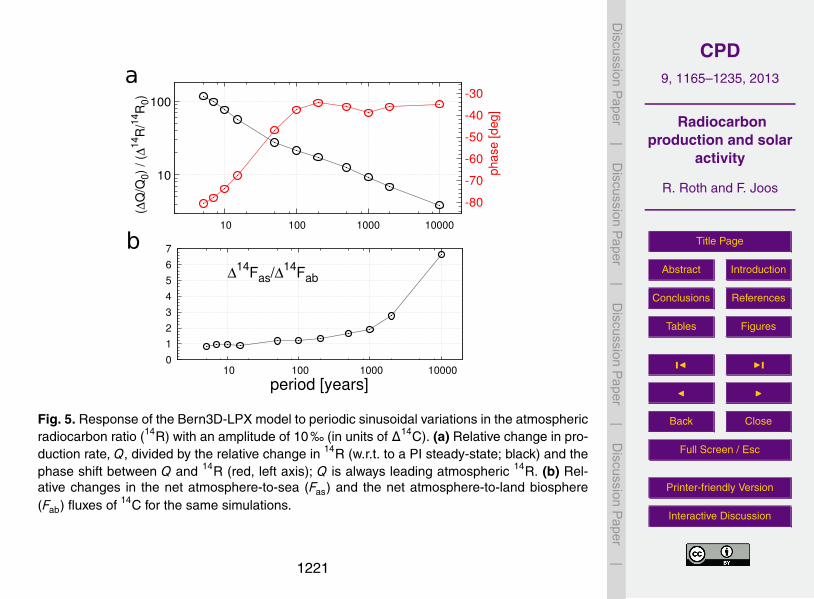
CPD9, 1165–1235, 2013


activity

R. Roth and F. Joos

Title Page



Tables Figures

J I

J I

Back Close

Full Screen / Esc



Discussion

Paper

|D

iscussionP

aper|

Discussion

Paper

|D

iscussionP

aper|

Discu

ssionPaper

|Discu

ssionPaper

|Discu

ssionPaper

|Discu

ssionPaper

|

a

period [years]

Δ14Fas/Δ14Fab

0

1

2

3

4

5

6

7

10 100 1000 10000

(ΔQ

/Q0)

/ (Δ

14R

/14R

0)

phase

[deg]

10

100

-80

-70

-60

-50

-40

-30

10 100 1000 10000

b

Fig. 5. Response of the Bern3D-LPX model to periodic sinusoidal variations in the atmospheric radio-carbon ratio (14R) with an amplitude of 10‰ (in units of ∆14C). (a) Relative change in productionrate, Q, divided by the relative change in 14R (w.r.t. to a PI steady-state; black) and the phase shiftbetween Q and 14R (red, left axis); Q is always leading atmospheric 14R. (b) Relative changes in thenet atmosphere-to-sea (Fas) and the net atmosphere-to-land biosphere (Fab) fluxes of 14C for the samesimulations.

52

Fig. 5. Response of the Bern3D-LPX model to periodic sinusoidal variations in the atmosphericradiocarbon ratio (14R) with an amplitude of 10 ‰ (in units of ∆14C). (a) Relative change in pro-duction rate, Q, divided by the relative change in 14R (w.r.t. to a PI steady-state; black) and thephase shift between Q and 14R (red, left axis); Q is always leading atmospheric 14R. (b) Rel-ative changes in the net atmosphere-to-sea (Fas) and the net atmosphere-to-land biosphere(Fab) fluxes of 14C for the same simulations.

1221





CPD9, 1165–1235, 2013


activity

R. Roth and F. Joos

Title Page



Tables Figures

J I

J I

Back Close

Full Screen / Esc



Discussion

Paper

|D

iscussionP

aper|

Discussion

Paper

|D

iscussionP

aper|

Discu

ssionPaper

|Discu

ssionPaper

|Discu

ssionPaper

|Discu

ssionPaper

|SAT [oC]BIO

CIRC3.06.09.0

12.015.0

deep ocean B-P ventilation age [kyrs]

0.51.01.52.02.53.0

missing CO2-flux [GtC/yr]-1.0-0.50.00.51.0

cumulative missing CO2-flux [GtC]

020004000600080001000012000140001600018000

0.0500.01000.01500.0

13.013.313.613.914.214.5

missing CO2-flux [GtC/yr]

1000 1100 1200 1300 1400 1500 1600 1700 1800 1900-1.5-1.0-0.50.00.51.01.5

time [yr B.P.]

time [yr A.D.]

CTL

SAT [oC]

a

b

c

d

e

f

Fig. 6. Transient model response of (a) surface atmospheric temperature (SAT), (b) global averaged B-Preservoir age calculated as 14C-age offset from the global ocean below 2000 m relative to the overlyingsurface ocean, (c) implied carbon flux to solve the atmospheric budget (Fbudget) and cumulative sumthereof (d) for the experiments BIO, CIRC and the control-run CTL. For the last millennium, SAT andFbudget is shown in detail in the lower two panels (e-f).

53

Fig. 6. Transient model response of (a) surface atmospheric temperature (SAT), (b) globalaveraged B-P reservoir age calculated as 14C-age offset from the global ocean below 2000 mrelative to the overlying surface ocean, (c) implied carbon flux to solve the atmospheric budget(Fbudget) and cumulative sum thereof (d) for the experiments BIO, CIRC and the control-runCTL. For the last millennium, SAT and Fbudget is shown in detail in the lower two panels (e, f).

1222





CPD9, 1165–1235, 2013


activity

R. Roth and F. Joos

Title Page



Tables Figures

J I

J I

Back Close

Full Screen / Esc



Discussion

Paper

|D

iscussionP

aper|

Discussion

Paper

|D

iscussionP

aper|

Discu

ssionPaper

|Discu

ssionPaper

|Discu

ssionPaper

|Discu

ssionPaper

|

model

data

model -data

DI14C [μmol/l/14RSTD]

N

N

Fig. 7. Comparison of modern modelled and data-based (GLODAP,WOA09) oceanic distribution of14C in its dominant form of dissolved inorganic carbon (DI14C) along a transect through the Atlantic,Southern Ocean and Pacific. The lowest panel shows the model-data difference.

54

Fig. 7. Comparison of modern modelled and data-based (GLODAP,WOA09) oceanic distribu-tion of 14C in its dominant form of dissolved inorganic carbon (DI14C) along a transect throughthe Atlantic, Southern Ocean and Pacific. The lowest panel shows the model-data difference.

1223





CPD9, 1165–1235, 2013


activity

R. Roth and F. Joos

Title Page



Tables Figures

J I

J I

Back Close

Full Screen / Esc



Discussion

Paper

|D

iscussionP

aper|

Discussion

Paper

|D

iscussionP

aper|

Discu

ssionPaper

|Discu

ssionPaper

|Discu

ssionPaper

|Discu

ssionPaper

|

a

b

c

d

e

CTLCIRC BIO

-100.0

-50.0

0.0

50.0

100.0

14abF

F-100.0

-50.0

0.0

50.0

100.0

14as

time [year B.P.]0200040006000800010000

400.0

450.0

500.0

550.0

600.0

650.0

time [year A.D.]

INT09

CTL CIRC BIO350.0

400.0

450.0

500.0

550.0

600.0

1000 1100 1200 1300 1400 1500 1600 1700 1800 1900

atmosphere

total

total

units: [mol/yr]

360.0

390.0

420.0

450.0

480.0

510.0

540.0

Fig. 8. Holocene 14C fluxes in mol 14C/yr for the different experiments: (a) Changes and decay of theatmospheric inventory (including Fbudget), (b) air-biosphere flux (Fab), (c) air-sea flux (Fas) and (d)the sum of these contributions yielding the total production rate Q. Panel (e) shows the last 1000 yrs ingreater detail together with an experiment (INT09) where the entire globe is forced with the northern-hemisphere dataset IntCal09 (dashed line), thereby neglecting the interhemispheric gradient in ∆14C.Note that the timeseries shown in panels a&b have been smoothed with a cutoff of 40 yrs (only for thevisualization) while panels c-e show 20 yrs smoothed data as described in the main text.

55

Fig. 8. Holocene 14C fluxes in mol14Cyr−1 for the different experiments: (a) changes and decayof the atmospheric inventory (including Fbudget), (b) air-biosphere flux (Fab), (c) air-sea flux (Fas)and (d) the sum of these contributions yielding the total production rate Q. Panel (e) showsthe last 1000 yr in greater detail together with an experiment (INT09) where the entire globeis forced with the Northern Hemisphere dataset IntCal09 (dashed line), thereby neglectingthe interhemispheric gradient in ∆14C. Note that the timeseries shown in (a) and (b) havebeen smoothed with a cutoff of 40 yr (only for the visualization) while panels (c)–(e) show 20 yrsmoothed data as described in the main text.

1224





CPD9, 1165–1235, 2013


activity

R. Roth and F. Joos

Title Page



Tables Figures

J I

J I

Back Close

Full Screen / Esc



Discussion

Paper

|D

iscussionP

aper|

Discussion

Paper

|D

iscussionP

aper|

Discu

ssionPaper

|Discu

ssionPaper

|Discu

ssionPaper

|Discu

ssionPaper

|14C decay

CIRCBIO

420.0

440.0

460.0

480.0

change in14

C inventory-150.0

-100.0

-50.0

0.0

50.0

100.0

sedimentary processes

50.0

60.0

70.0

80.0

time [year B.P.]

total40005000600070008000900010000110001200013000

350.0400.0450.0500.0550.0600.0650.0

units: [mol/yr]a

b

c

d

Fig. 9. The oceanic 14C budget for the experiments BIO and CIRC for the last part of the glacial termina-tion I and the early Holocene. (a) Decay of the data-normalized inventory of 14C in the form of inorganicand organic carbon, (b) changes in whole ocean radiocarbon inventory, (c) contribution from sediments(burial flux and decay of 14C within the active sediment layer). After 4 kyr BP, the two experiments donot show significant differences in the total ocean-sediment 14C loss (panel d).

56

Fig. 9. The oceanic 14C budget for the experiments BIO and CIRC for the last part of theglacial termination I and the early Holocene. (a) Decay of the data-normalized inventory of14C in the form of inorganic and organic carbon, (b) changes in whole ocean radiocarbon in-ventory, (c) contribution from sediments (burial flux and decay of 14C within the active sedimentlayer). After 4 kyrBP, the two experiments do not show significant differences in the total ocean-sediment 14C loss (d).

1225





CPD9, 1165–1235, 2013


activity

R. Roth and F. Joos

Title Page



Tables Figures

J I

J I

Back Close

Full Screen / Esc



Discussion

Paper

|D

iscussionP

aper|

Discussion

Paper

|D

iscussionP

aper|

Discu

ssionPaper

|Discu

ssionPaper

|Discu

ssionPaper

|Discu

ssionPaper

|m

ole

s/yr

ato

ms/

cm

2/s

time [yr B.P.]

this study Marmod09 US05

250

300

350

400

450

500

550

600

650

5000600070008000900010000

1

1.2

1.4

1.6

1.8

2

2.2

2.4

mo

les/

yr

ato

ms/

cm2/s

time [yr B.P.]

250

300

350

400

450

500

550

600

650

010002000300040005000

1

1.2

1.4

1.6

1.8

2

2.2

2.4

mo

les/y

r

ato

ms/c

m2/s

time [yr A.D.]

this study Marmod09 US05

250

300

350

400

450

500

550

600

1000 1100 1200 1300 1400 1500 1600 1700 1800 1900

1

1.2

1.4

1.6

1.8

2

2.2

a

b

c

Fig. 10. (a-b) Total 14C production rate from this study (black line with gray 1σ shading) and the re-constructions from Usoskin and Kromer (2005) (violet) and the output of the Marmod09 box-model(red). The gray shading indicates ± 1σ uncertainty as computed from statistical uncertainties in the at-mospheric ∆14C records, in the processes governing the deglacial CO2 increase, air-sea gas transfer rateand global primary production on land (see appendix and Fig. A1). Panel (c) shows the last 1000 yearsof the production record in more detail.

57

Fig. 10. (a, b) Total 14C production rate from this study (black line with gray 1σ shading) andthe reconstructions from Usoskin and Kromer (2005) (violet) and the output of the Marmod09box-model (red). The gray shading indicates ±1σ uncertainty as computed from statisticaluncertainties in the atmospheric ∆14C records, in the processes governing the deglacial CO2increase, air–sea gas transfer rate and global primary production on land (see Appendix andFig. A1). (c) Shows the last 1000 yr of the production record in more detail.

1226





CPD9, 1165–1235, 2013


activity

R. Roth and F. Joos

Title Page



Tables Figures

J I

J I

Back Close

Full Screen / Esc



Discussion

Paper

|D

iscussionP

aper|

Discussion

Paper

|D

iscussionP

aper|

Discu

ssionPaper

|Discu

ssionPaper

|Discu

ssionPaper

|Discu

ssionPaper

|

0200040006000800010000

time [year B.P.]

4

6

8

10

12

14V

AD

M [

1022

Am2

]

Yang et al.,2000 (YN00)Knudsen et al., 2008 (KN08)Korte et al., 2011 (KO11)

Jackson et al.,2000

Fig. 11. Reconstructions of the virtual axis dipole moment (VADM) of the geomagnetic field for theHolocene. Black: Yang et al. (2000), orange: Knudsen et al. (2008), blue: Korte et al. (2011). For themost recent epoch the estimate of Jackson et al. (2000) yields 8.22×1022 Am2 (red dot). In the presentstudy, the data of Korte et al. (2011) is used.

58

Fig. 11. Reconstructions of the virtual axis dipole moment (VADM) of the geomagnetic fieldfor the Holocene. Black: Yang et al. (2000), orange: Knudsen et al. (2008), blue: Korte et al.(2011). For the most recent epoch the estimate of Jackson et al. (2000) yields 8.22×1022 Am2

(red dot). In the present study, the data of Korte et al. (2011) is used.

1227





CPD9, 1165–1235, 2013


activity

R. Roth and F. Joos

Title Page



Tables Figures

J I

J I

Back Close

Full Screen / Esc



Discussion

Paper

|D

iscussionP

aper|

Discussion

Paper

|D

iscussionP

aper|

Discu

ssionPaper

|Discu

ssionPaper

|Discu

ssionPaper

|Discu

ssionPaper

|

Φ[M

eV

]

time [yr B.P.]

this study US07 SEA08

0

200

400

600

800

1000

1200

5000600070008000900010000

Φ[M

eV

]

time [yr B.P.]

0

200

400

600

800

1000

1200

010002000300040005000

Φ[M

eV

]

time [yr A.D.]

US11 US07 MEA07 SEA08

0

200

400

600

800

1000

1200

1400

1000 1200 1400 1600 1800 2000

a

b

c

Fig. 12. (a-b) Solar modulation potential Φ based on the reconstructed radiocarbon production and theVADM history of Korte et al. (2011). The Φ-histories of Usoskin et al. (2007) (US07,blue) and of Stein-hilber et al. (2008) (SEA08,red) are shown additionally. For the last millennium (panel c), we includethe Φ record from Muscheler et al. (2007) (MEA07,green) as well as the instrumental data compiledby Usoskin et al. (2011) (US11,violet). The latter was used for normalization and extension of our Φreconstruction over recent decades. Note that all Φ’s are normalized to the LIS of Castagnoli and Lal(1980) for according to Herbst et al. (2010).

59

Fig. 12. (a, b) Solar modulation potential Φ based on the reconstructed radiocarbon productionand the VADM history of Korte et al. (2011). The Φ-histories of Usoskin et al. (2007) (US07,blue) and of Steinhilber et al. (2008) (SEA08, red) are shown additionally. For the last millen-nium (c), we include the Φ record from Muscheler et al. (2007) (MEA07, green) as well asthe instrumental data compiled by Usoskin et al. (2011) (US11, violet). The latter was used fornormalization and extension of our Φ reconstruction over recent decades. Note that all Φ’s arenormalized to the LIS of Castagnoli and Lal (1980) for according to Herbst et al. (2010).

1228





CPD9, 1165–1235, 2013


activity

R. Roth and F. Joos

Title Page



Tables Figures

J I

J I

Back Close

Full Screen / Esc



Discussion

Paper

|D

iscussionP

aper|

Discussion

Paper

|D

iscussionP

aper|

Discu

ssionPaper

|Discu

ssionPaper

|Discu

ssionPaper

|Discu

ssionPaper

|

6.0 6.5 7.0 7.5 8.0 8.5 9.0 9.5 10.0

geomagnetic field intensity [1022Am2 ]

200

300

400

500

600

700

800

900

sola

r m

odula

tion f

un

ctio

n [

MeV

]

1.41.5

1.6

1.7

1.8

1.92.0

2.12.22.3

count

count200

300

400

500

600

700

800

900

Fig. 13. The absolute radiocarbon production rate plotted as a function of the solar modulation parameterΦ and VADM. Yearly values of the smoothed Q record are used (with a cutoff period of 20 yrs as in Fig.10). The path taken by the model in this (Φ,VADM)-space is indicated by the thin gray line. The circleshows the value of Φ for the normalization period 1937-1950 as reported by Usoskin et al. (2011). Thediamond shows the average production rate over the entire Holocene. On the sides of the figure, twohistograms are displayed showing the relative occurrence of certain VADM (top) and Φ (right) values,∼570 MeV being the most frequent modulation potential during the Holocene.

60

Fig. 13. The absolute radiocarbon production rate plotted as a function of the solar modulationparameter Φ and VADM. Yearly values of the smoothed Q record are used (with a cutoff periodof 20 yr as in Fig. 10). The path taken by the model in this (Φ,VADM)-space is indicated bythe thin gray line. The circle shows the value of Φ for the normalization period 1937–1950 asreported by Usoskin et al. (2011). The diamond shows the average production rate over theentire Holocene. On the sides of the figure, two histograms are displayed showing the relativeoccurrence of certain VADM (top panel) and Φ (right panel) values, ∼570 MeV being the mostfrequent modulation potential during the Holocene.

1229





CPD9, 1165–1235, 2013


activity

R. Roth and F. Joos

Title Page



Tables Figures

J I

J I

Back Close

Full Screen / Esc



Discussion

Paper

|D

iscussionP

aper|

Discussion

Paper

|D

iscussionP

aper|

Discu

ssionPaper

|Discu

ssionPaper

|Discu

ssionPaper

|Discu

ssionPaper

|

ΔT

SI [W

/m2]

time [yr B.P.]

this study VEA11 SEA12

-1.0

-0.5

0.0

0.5

1.0

5000600070008000900010000

ΔT

SI [W

/m2]

time [yr B.P.]

-1.0

-0.5

0.0

0.5

1.0

010002000300040005000

ΔT

SI [W

/m2]

time [yr A.D.]

this studyDB11

VEA11SEA12

PMOD

-1.0

-0.5

0.0

0.5

1.0

1000 1200 1400 1600 1800 2000

a

b

c

Fig. 14. (a-b) Total solar irradiance deviation from solar cycle minimum value in 1986 (assumed to1365.57 W/m2) calculated in this study (black with gray 1 σ error), the reconstruction by Vieira et al.(2011) (VEA11, red) and Steinhilber et al. (2012) (SEA12, blue). (c) Magnification of the last 1000years, in addition to VEA11 and SEA12 the data of Delaygue and Bard (2011) (DB11, green) is shownas well as the PMOD composite record.

61

Fig. 14. (a, b) Total solar irradiance deviation from solar cycle minimum value in 1986 (assumedto 1365.57 Wm−2) calculated in this study (black with gray 1 σ error), the reconstruction byVieira et al. (2011) (VEA11, red) and Steinhilber et al. (2012) (SEA12, blue). (c) Magnificationof the last 1000 yr, in addition to VEA11 and SEA12 the data of Delaygue and Bard (2011)(DB11, green) is shown as well as the PMOD composite record.

1230





CPD9, 1165–1235, 2013


activity

R. Roth and F. Joos

Title Page



Tables Figures

J I

J I

Back Close

Full Screen / Esc



Discussion

Paper

|D

iscussionP

aper|

Discussion

Paper

|D

iscussionP

aper|

Discu

ssionPaper

|Discu

ssionPaper

|Discu

ssionPaper

|Discu

ssionPaper

|

Period [yrs]Pe

riod [

yrs

]Pow

er

[a.u

.]ade Vries~210 yr

Eddy ~1000yrGleissberg~87 yr

b

c

0

5

10

15

20

100 1000

ΔT

SI [w

/m2]

-0.6-0.4-0.20.00.20.40.60.8

10000 9000 8000 7000 6000 5000 4000 3000 2000 1000

Time [year B.P.]

64

128

256

512

1024

2048

1/256

1/64

1/16

1/4

1

4

16

Pow

er

[a.u

.]

0

ΔT

SI [w

/m2]

time [yr A.D.]

-0.6

-0.4

-0.2

0.0

0.2

0.4

0.6

1500 1700 1900 2100 2300 2500

5000th order

1000th order

10000th orderpast future

Fig. 15. (a) Power spectrum our TSI record up to periodicities of 2000 yrs. The most dominant periodic-ities correspond to the Gleissberg, de Vries and Eddy cycles. (b) Wavlet power spectrum calculated witha Morlet-wavelet with log2 periodicity axis and color shading. (c) Extrapolation of the solar irradianceusing an auto-regressive (AR) model (Burg method) with different orders.

62

Fig. 15. (a) Power spectrum our TSI record up to periodicities of 2000 yr. The most dominant pe-riodicities correspond to the Gleissberg, de Vries and Eddy cycles. (b) Wavlet power spectrumcalculated with a Morlet-wavelet with log2 periodicity axis and color shading. (c) Extrapolationof the solar irradiance using an auto-regressive (AR) model (Burg method) with different orders.

1231





CPD9, 1165–1235, 2013


activity

R. Roth and F. Joos

Title Page



Tables Figures

J I

J I

Back Close

Full Screen / Esc



Discussion

Paper

|D

iscussionP

aper|

Discussion

Paper

|D

iscussionP

aper|

Discu

ssionPaper

|Discu

ssionPaper

|Discu

ssionPaper

|Discu

ssionPaper

|

ΔS

AT

[K

]

time [yr B.P.]

SEA12 VEA11 this study

-0.15

-0.10

-0.05

0.00

0.05

0.10

5000600070008000900010000

ΔS

AT

[K

]

time [yr B.P.]

-0.15

-0.10

-0.05

0.00

0.05

0.10

010002000300040005000

ΔS

AT

[K

]

time [yr A.D.]

SEA12 VEA11 this study

-0.15

-0.10

-0.05

0.00

0.05

0.10

1000 1200 1400 1600 1800 2000

a

b

c

Fig. 16. (a-b) Simulated changes in SAT as a response to different TSI forcings: This study (black),VEA11 (red) and SEA12 (blue). The anomalies were calculated as the difference between two transientsimulations, one with all forcings and the other with the same forcings but solar forcing taken to beconstant. The last 1000 yrs are shown again in panel (c). In all panels, thin lines show annual data whilethick lines show smoothing splines with a cutoff period of 50 yrs.

63

Fig. 16. (a, b) Simulated changes in SAT as a response to different TSI forcings: this study(black), VEA11 (red) and SEA12 (blue). The anomalies were calculated as the difference be-tween two transient simulations, one with all forcings and the other with the same forcings butsolar forcing taken to be constant. The last 1000 yr are shown again in panel (c). In all panels,thin lines show annual data while thick lines show smoothing splines with a cutoff period of50 yr.

1232





CPD9, 1165–1235, 2013


activity

R. Roth and F. Joos

Title Page



Tables Figures

J I

J I

Back Close

Full Screen / Esc



Discussion

Paper

|D

iscussionP

aper|

Discussion

Paper

|D

iscussionP

aper|

Discu

ssionPaper

|Discu

ssionPaper

|Discu

ssionPaper

|Discu

ssionPaper

|

total production rate

350.0400.0450.0500.0550.0600.0650.0700.0

error from Δ14C record

15.0

25.0

35.0

45.0

error from deglacial history

5.0

10.0

15.0

20.0

error from gas exchange/GPP

1.0

4.0

7.0

10.0

13.0

error from CO2-budget

0.0

5.0

10.0

15.0

time [year B.P.]

total error

20.030.040.050.0

0200040006000800010000

a

b

c

d

e

f

Fig. A1.1 Assessment of uncertainties in our production rate record. (a) Radiocarbon production rate(arithmetic mean of CIRC and BIO), (b) the uncertainty stemming from the pre-Holocene carbon-cycleevolution calculated as the absolute difference between results from simulations BIO and CIRC, (c) thesmoothed 1σ error from the ∆14C record (as shown in Fig. 2b) is calculated by a Monte-Carlo approach

including 100 individual simulations and (d) the uncertainty in air-sea and air-land fluxes deduced bysensitivity experiments. The total error in production (panel e) varies between 50 and 10 mol/yr,corresponding to a relative error of ∼10 to 2.5 %. The bulk uncertainty in the average level of Q

resulting form an uncertain ocean (and land) inventory is not included in this calculation. We estimatethis uncertainty to be ∼15%.

66

Fig. A1. Assessment of uncertainties in our production rate record. (a) Radiocarbon productionrate (arithmetic mean of CIRC and BIO), (b) the uncertainty stemming from the pre-Holocenecarbon-cycle evolution calculated as the absolute difference between results from simulationsBIO and CIRC, (c) the smoothed 1σ error from the ∆14C record (as shown in Fig. 2b) is calcu-lated by a Monte-Carlo approach including 100 individual simulations and (d) the uncertaintyin air–sea and air–land fluxes deduced by sensitivity experiments. The total error in production(e) varies between 50 and 10 molyr−1, corresponding to a relative error of ∼10 to 2.5 %. Thebulk uncertainty in the average level of Q resulting form an uncertain ocean (and land) inventoryis not included in this calculation. We estimate this uncertainty to be ∼15 %.

1233





CPD9, 1165–1235, 2013


activity

R. Roth and F. Joos

Title Page



Tables Figures

J I

J I

Back Close

Full Screen / Esc



Discussion

Paper

|D

iscussionP

aper|

Discussion

Paper

|D

iscussionP

aper|

Discu

ssionPaper

|Discu

ssionPaper

|Discu

ssionPaper

|Discu

ssionPaper

|

Φ

0.0

200.0

400.0

600.0

800.0

1000.0

1200.0

error from Q

50.0

100.0

150.0

200.0

error from VADM

50.0

100.0

150.0

200.0

error from production model

20.0

40.0

60.0

80.0

100.0

time [year B.P.]

total error

50.0100.0150.0200.0250.0300.0

0200040006000800010000

a

b

c

d

e

Fig. A2.1 Assessment of uncertainties in the solar modulation potentialΦ. (a) Best estimate of Φ (meanof the Monte-Carlo simulations), (b) uncertainty in Φ from uncertainties in the radiocarbon productionQ, (c) from the uncertainty in the VADM reconstruction by Korte et al. (2011), (d) the uncertainty in the

model to convert production into Φ, and (e) total 1σ uncertainty in the MC calculation.

67

Fig. A2. Assessment of uncertainties in the solar modulation potentialΦ. (a) Best estimate ofΦ (mean of the Monte-Carlo simulations), (b) uncertainty in Φ from uncertainties in the radio-carbon production Q, (c) from the uncertainty in the VADM reconstruction by Korte et al. (2011),(d) the uncertainty in the model to convert production into Φ, and (e) total 1σ uncertainty in theMC calculation.

1234





CPD9, 1165–1235, 2013


activity

R. Roth and F. Joos

Title Page



Tables Figures

J I

J I

Back Close

Full Screen / Esc



Discussion

Paper

|D

iscussionP

aper|

Discussion

Paper

|D

iscussionP

aper|

Discu

ssionPaper

|Discu

ssionPaper

|Discu

ssionPaper

|Discu

ssionPaper

|ΔTSI

-0.80-0.60-0.40-0.200.000.200.400.600.801.001.20

error from Φ

0.10

0.20

0.30

0.40

0.50

error from Φ-TSI relationship

0.10

0.20

0.30

0.40

0.50

time [year B.P.]

total error

0.200.300.400.500.600.70

0200040006000800010000

a

b

c

d

Fig. A2.2 Assessment of uncertainties in the ∆TSI reconstruction in W/m2. (a) ∆TSI (mean of theMonte-Carlo simulations), (b) the uncertainty in ∆TSI from the error of Φ, (c) from the uncertainty in

the TSI-Br relationship, and (d) when considering all uncertainties in the MC calculation. Errors are 1σuncertainties.

68

Fig. A3. Assessment of uncertainties in the ∆TSI reconstruction in Wm−2. (a) ∆TSI (mean ofthe Monte-Carlo simulations), (b) the uncertainty in ∆TSI from the error of Φ, (c) from theuncertainty in the TSI-Br relationship, and (d) when considering all uncertainties in the MCcalculation. Errors are 1σ uncertainties.

1235





Documents

A reconstruction of radiocarbon production and total solar irradiance from the Holocene 14C and CO2 records: implications of data and