A sequential Bayesian approach to color constancy using non-uniform filters

UNCORRECTEDPROOF

1

2 A sequential Bayesian approach to color constancy using non-uniform filters

3 Sandra Skaff *, Tal Arbel, James J. Clark

4 Centre for Intelligent Machines, McGill University, Montréal, Que., Canada H3A 2A7

5

7a r t i c l e i n f o

8 Article history:9 Received 20 June 2008

10 Accepted 25 March 200911 Available online xxxx

12 Keywords:13 Color constancy14 Bayesian15 Sequential: chaining16 Posterior17 Prior18 Filters: binary19 Multiple20

2 1

a b s t r a c t

22This paper introduces a non-uniform filter formulation into the Brainard and Freeman Bayesian color23constancy technique. The formulation comprises sensor measurements taken through a non-uniform fil-24ter, of spatially-varying spectral sensitivity, placed on the camera lens. The main goal of this paper is two-25fold. First, it presents a framework in which sensor measurements obtained through a non-uniform filter26can be sequentially incorporated into the Bayesian probabilistic formulation. Second, it shows that such27additional measurements obtained reduce the effect of the prior in Bayesian color constancy. For the pur-28poses of testing the proposed framework, we use a filter formulation of two portions of different spectral29sensitivities. We show through experiments on real data that improvement in the parameter estimation30can be obtained inexpensively by sequentially incorporating additional information obtained from the31sensor through the different portions of a filter by Bayesian chaining. We also show that our approach32outperforms previous approaches in the literature.33� 2009 Published by Elsevier Inc.

34

35

36 1. Introduction

37 Color constancy is the ability of a vision system to compute a38 measure of a surface’s color that is independent of the spectrum39 of the light incident on the surface. The human visual system has40 an effective, if imperfect, color constancy mechanism. Studies of41 the human color constancy system have led to the development42 of many color constancy methods for machine vision applications.43 None of the existing color constancy techniques function perfectly44 in all situations, and most fail outside of a limited domain of appli-45 cability. The difficulty in solving the color constancy problem lies46 in the bilinear nature of the underlying relation between the illu-47 minant and surface reflectance spectra and the measurements pro-48 vided by the photoreceptors. Perhaps the most successful methods49 of dealing with the inherent ambiguity induced by the bilinearity50 of the problem employ regularization techniques. A notable exam-51 ple of this can be found in Brainard and Freeman’s Bayesian tech-52 nique [1].53 One of the advantages of the Bayesian approach to solving the54 color constancy problem is that it permits a straightforward inte-55 gration of multiple sources of information. A drawback of any56 Bayesian method is the need to specify a prior distribution on57 the solution space, and the bias induced by the particular choice58 of prior. If more information, in the form of additional independent59 measurements, is provided, the influence of the prior is reduced.60 Studies of the human visual system reveal a possible source for this

61extra information. In looking at the structure of the retina, it is62clear that the spectral sensitivity of the photoreceptors is not uni-63form across the retina. Because of the effects of the macular pig-64ment, as well as the varying path length of light rays through the65lens material, the foveal photoreceptors are less sensitive to blue66wavelengths than the photoreceptors in the periphery. Despite67this, the human perception of color is invariant to eye position.68This means that we perceive the same color of an item both periph-69erally and foveally. One explanation for this invariance of color70perception across the retina is that the visual system is applying71a perceptual-stability constraint. A theory of how this could be72accomplished was proposed by Clark and O’Regan [2]. They sug-73gested that moving the eye results in a variation in the retinal sig-74nal. This variation, under the assumption that the world itself is not75changing, allows for the generation of a signal for adaptation,76which can be used to drive learning of invariance. Once invariance77is learned, the system will produce the same percept of color no78matter on which part of the retina the stimulus falls.79We incorporate the intuition provided by the Clark–O’Regan80color stability theory into the Brainard and Freeman Bayesian tech-81nique. A non-uniform filter with spatially-varying spectral sensi-82tivity can be used to represent the photoreceptors at different83retinal locations. Measurements can be obtained sequentially by84moving the gaze across a surface in the scene. These measurements85can be used to update the inference resulting from our Bayesian86formulation. Moreover, we propose to acquire multiple images of87the same scene by moving the camera. This camera motion also al-88lows for acquiring additional measurements which can be used to89reduce the effect of the prior in the Bayesian formulation. A major90advantage of our approach is that it does not require all surface

1077-3142/$ - see front matter � 2009 Published by Elsevier Inc.

doi:10.1016/j.cviu.2009.03.014

* Corresponding author.

E-mail addresses: [email protected] (S. Skaff), [email protected] (T. Arbel),

[email protected] (J.J. Clark).

Computer Vision and Image Understanding xxx (2009) xxx–xxx

Contents lists available at ScienceDirect

Computer Vision and Image Understanding

journal homepage: www.elsevier .com/ locate/cviu

YCVIU 1538 No. of Pages 12, Model 5G

10 April 2009 Disk UsedARTICLE IN PRESS

Please cite this article in press as: S. Skaff et al., A sequential Bayesian approach to color constancy using non-uniform filters, Comput. Vis. Image

Understand. (2009), doi:10.1016/j.cviu.2009.03.014

mailto:[email protected]



http://www.sciencedirect.com/science/journal/10773142

http://www.elsevier.com/locate/cviu

UNCORRECTEDPROOF

91 patches in the scene to be viewed through the whole filter. In other92 words, some patches can be viewed through one portion of the fil-93 ter but not another.94 All color constancy approaches, including the proposed one,95 have a limited domain of applicability which is usually defined96 by a set of assumptions. In this paper, we also have a set of97 assumptions that are stated up front to make it simpler for the98 reader to follow through the derivations later on in this paper.99 First, it is assumed that the surfaces are Mondrian [3]. A Mondrian

100 is a planar surface composed of several, overlapping, matte,101 patches named after the style of painting produced by the artist102 Piet Mondrian. Also, the surface patches are uniform and are103 uncorrelated from each other. Next, it is assumed that the sensor104 measurements obtained through the different portions of the filter105 are statistically independent from each other. In the case of obtain-106 ing measurements through different portions of the filter for the107 same surface, the independence assumption is still applied. In this108 case, one can think of the different parts of the surface viewed109 through different portions of the filter as different surfaces. The110 fact that they have the same underlying spectra does not necessar-111 ily imply that they are parts of the same surface. Moreover, it is as-112 sumed that each sensor measurement comprises three statistically113 independent measurements for the three sensor types: Red ðRÞ,114 Green ðGÞ, and Blue ðBÞ. Furthermore, the light illuminating a Mon-115 drian scene is assumed to be locally constant; that is the spectral116 characteristics of the light vary slowly. Therefore, the spectrum117 of light falling on the lens does not vary with viewpoint for one118 surface patch, and any change in measurements after moving the119 sensors would be due to noise. However, it is assumed that these120 measurements are constant. Note that assuming constant illumi-121 nation across a scene is a common practice in color constancy ap-122 proaches [4]. Moreover, since the surface patches are flat in nature123 and they are placed on a flat surface, there are no interreflections124 between them. This means that a surface spectral reflectance and125 the illuminant spectrum vectors are sufficient statistics for the126 measurements of the corresponding single surface patch. Further-127 more, it is assumed that segmentation and correspondence tasks128 have already been run on the images, and therefore we know129 which surface patches are viewed through which portions of the130 filter. Finally, note that while the assumptions stated above may131 impose practical limitations, we show in this paper that our ap-132 proach can still be applied successfully to real image data.133 This paper is organized as follows. First, color constancy ap-134 proaches which use linear model representations for surface and135 illuminant spectra are summarized in Section 2. The Bayesian ap-136 proach is detailed in this section as well. Next, the proposed ap-137 proach is explained and derived in Section 3. For the purposes of138 testing the proposed approach on real data, a filter formulation139 of two spectral sensitivities is used. Section 4 shows experimental140 results on real data where improvement in illuminant and surface141 spectral estimation is attained by incorporating additional sensor142 measurements through filter portions of different spectral sensitiv-143 ities. Section 5 compares the proposed approach to state-of-the-art144 approaches in the literature. The paper is concluded in Section 6.

145 2. Linear color constancy algorithms

146 Many color constancy algorithms lie in computing surface and147 illuminant spectra, which are represented by linear models. Such148 representations appear in Brill and West’s work [5] on von Kries149 adaptation [6], which is the oldest algorithm for color constancy.150 These representations also appear in Buchsbaum’s [7] and Gershon151 et al.’s work [8], who proposed variants of the gray world algo-152 rithm, which assumed that the average of the surface reflectances153 in the scene is gray. Since this assumption can be easily violated,

154these approaches do not perform well in practice. Linear model155representations also appear in Maloney and Wandell [9,10] and156Yuille’s work [11], in which the assumption of having more photo-157receptor responses than the number of surface and illuminant158spectra basis functions is required. This is a serious limitation,159especially in estimating surface spectra. It implies that no more160than three basis functions can be used in the event that the rod161photoreceptor response is used in addition to those of the cones.162D’Zmura and Lennie [12] and D’Zmura and Iverson [13,14] also163used linear model representations for surface and illuminant spec-164tra. The authors in [13,14] proposed a model check algorithm to165determine necessary and sufficient conditions for unique recovery166of surface and illuminant spectra. Another approach is Ho et al.’s167[15], which estimates surface and illuminant spectra using linear168model representations from the color signal as opposed to the pho-169toreceptor response. This signal, which is the product of the illumi-170nant and surface spectra, needs to be measured using a171spectroradiometer if the approach were to be applied on real data.172The issues in all the approaches mentioned above led us to base173our work on Brainard and Freeman’s approach [1], which estimates174surface and illuminant spectral basis function weights from photo-175receptor responses. This approach, explained in Section 2.1, im-176poses no restrictions on the number of surface spectra basis177functions compared to the number of photoreceptor responses.178The novelty of our approach lies in showing how surface and illu-179minant spectra can be used to inexpensively accumulate informa-180tion obtained from the sensor through filter portions, of different181spectral sensitivities, using the Bayesian framework.

1822.1. Bayesian color constancy

183Brainard and Freeman used a regularization technique to solve184the problem of computing the values of the illuminant and surface185reflectance spectra parameters [1]. The regularization technique186used is based on Bayesian inference [16,17]. The advantage of using187the Bayesian model is that it embeds all possible uncertainties as188probability distributions, and that it performs inference based on189all the information available in the data. For a given problem, the190Bayesian approach makes use of a priori information about likely191physical configurations of the solution. It is this prior information192that helps in resolving ambiguities in the problem. Therefore, in this193sense, the Bayesian approach can be thought of as a regularizer of194the problem to obtain the solution in question. On the other hand,195the drawbacks of using the Bayesian method should be taken into196consideration. First, it may be difficult to specify a prior distribu-197tion. Also, in the event of maximizing the posterior, it may be diffi-198cult to specify a suitable cost function for the optimization process199and, furthermore, this function may be difficult to maximize.200The surface and illuminant spectra in the Bayesian color con-201stancy approach are parametrized using Maloney and Wandell’s202bilinear model [10]. The authors in [10] proposed an algorithm203for computing the model parameters from sensor measurements204of the light reflected from a set of surface patches. They start by205describing the spectrum of light arriving at location x on an array206of sensors by the function:

IxðkÞ ¼ EðkÞSxðkÞ; ð1Þ 208208

209where EðkÞ is the spectral power distribution of the ambient light in210the scene, SxðkÞ is the surface spectral reflectance, and k denotes the211wavelength. Assuming that there are p sensors at each location x,212and the relative wavelength sensitivity of the k

thsensor is RkðkÞ,

213the response recorded at each location is given by214

qxk ¼

X

M

k¼1

EðkÞSxðkÞRkðkÞdk; k ¼ 1;2; . . . ;p; ð2Þ216216

2 S. Skaff et al. / Computer Vision and Image Understanding xxx (2009) xxx–xxx





UNCORRECTEDPROOF

217 where M denotes the dimensionality of the spectra. S and E are rep-218 resented as linear models with n and m basis functions,219 respectively:220

SxðkÞ ¼X

n

j¼1

rxj SjðkÞ; ð3Þ

EðkÞ ¼X

m

i¼1

�iEiðkÞ: ð4Þ222222

223 In both cases, the basis functions are fixed and are assumed to be224 known. The basis functions for the surface reflectances, SjðkÞ, are225 computed using principal components analysis (PCA) on a set of226 150 Munsell color chips. Munsell patches can be found in the Mun-227 sell Book of Color [18]. The basis functions of the light spectra EiðkÞ

228 are computed using PCA on a set of 622 different spectra of natural229 daylight. Therefore, to find the surface reflectance and ambient230 light, the basis function weights rx

j and �i should be computed.231 The sensor responses can be viewed as bilinear functions of the un-232 known basis function weights. This bilinearity means that various233 choices of � and rx can produce identical sensor measurements234 and, therefore, that the problem of finding the weights is ill-posed.235 Substituting Eqs. (3) and (4) into Eq. (2) yields the following236 equation:237

qxk ¼

X

n

j¼1

rxj SjðkÞ

X

m

i¼1

�iEiðkÞRkðkÞdk; k ¼ 1;2; . . . ; p: ð5Þ239239

240 Maloney and Wandell assumed that a surface spectrum can be241 modeled by only two basis functions although this is a severe con-242 straint. The authors require such an assumption because their algo-243 rithm requires more sensors than surface basis functions, and there244 are only three sensors: red, green, and blue. This assumption limits245 the results when the algorithm is presented with surfaces that can-246 not be represented accurately by only two basis functions. For247 example, Parkkinen et al. showed that Munsell patch spectra need248 as many as eight basis functions to achieve an accurate representa-249 tion [19]. However, taking into account the fact that the first few250 principal components contain the most information in general, this251 assumption might not pose a problem in some cases.252 Bayesian inference theory is comprised of three probability253 density functions: the prior, the posterior, and the likelihood. We254 denote the vector of the surface and illumination spectra model255 weights as ~w, and the sensor responses as ~y. We can obtain a sta-256 tistical model for ~w by the conditional posterior density function of257 ~w given the measurement ~y as pð~wj~yÞ such that

pð~wj~yÞ ¼pð~yj~wÞpð~wÞ

pð~yÞ/ pð~yj~wÞpð~wÞ: ð6Þ

259259

260 pð~yj~wÞ is the likelihood which models the relationship between the261 illuminant and surface spectra model weights and the sensor re-262 sponses. pð~wÞ represents the prior information on the model param-263 eters. pð~yÞ represents the probability of the sensor responses or the264 measurements and is a normalization term that does not affect the265 shape of the posterior distribution. In the Brainard–Freeman formu-266 lation, the prior is represented by a normal distribution on the267 weights of the illuminant and surface reflectance spectra. These268 weights are computed by projecting these illuminant and surface269 reflectance spectra vectors on the illuminant and surface reflectance270 spectra basis functions. The illuminant data set is composed of day-271 light spectra with temperatures ranging from 3000 to 25,000 K,272 while the surface data set is composed of Munsell reflectance spec-273 tra. The likelihood pð~yj~wÞ is also represented by a normal distribu-274 tion. Given the posterior pð~wj~yÞ, they compute a loss function275 which they call the Bayesian expected loss:

Lð ~~wj~yÞ ¼

Z

~w

Lð ~~wj~wÞpð~wj~yÞdw: ð7Þ277277

278This function computes the penalty for choosing a single estimate ~~w279when the actual parameters are ~w [16]. Brainard and Freeman280choose an estimate for ~w such that the loss is minimal. They discuss281three types of loss functions: the Maximum A Posteriori (MAP), the282Minimum Mean Squared Error (MMSE), and the Maximum Local283Mass (MLM). For simplicity in this paper, we choose to use the284MAP function.

2853. The sequential non-uniform filter formulation

286We introduce a technique that builds upon Brainard and Free-287man’s Bayesian approach in which only one sensor response is ac-288quired. Our technique acquires sensor measurements through289different filter portions, each having its own spectral sensitivity.290Therefore, the inherent ill-posedness of the problem is addressed291through the introduction of more sources of information. This292acquisition of measurements is similar to when a person moves293his/her gaze across a scene and is inspired by Clark and O’Regan’s294theory of color stability [2]. This theory states that the human’s per-295ception of color is invariant to eye position. The acquisition of296information is sequential and can be modeled through a sequential297Bayesian estimation process. Note that this process is computa-298tionally feasible as its complexity lies in the multiple computations299of the probability density functions of the Bayesian formulation.300We had shown in simulation in [20] that there is improvement301in the surface patch spectra estimates with the placement of a non-302uniform filter on the camera lens. Two types of filters were consid-303ered: one with two portions, each having a different spectral sen-304sitivity characteristic, and one with more than two portions. The305latter formulation was chosen to be Gaussian as it mimics the var-306iation in the spectral sensitivity of the photoreceptors across the307retina. This Gaussian formulation could be constructed with a drop308of food coloring placed on transparent glass. Therefore, this filter309would have spectral transmittance that is maximum in the center310and that decreases gradually toward the peripheries. However,311constructing such a filter is beyond the scope of this paper. There-312fore, in order to show how acquiring additional measurements im-313proves on spectral estimation, we use a filter of two portions with314two corresponding spectral sensitivities here.315As in the Brainard and Freeman approach, evidence for the316lighting and surface color parameters of either one or many surface317patches in a scene is represented by a conditional probability den-318sity function given the sensor measurements. Since there are two319distinct portions of the filter, X and Y, this probabilistic evidence320is then accumulated sequentially over X and Y. In practice, this for-321mulation can be modeled by placing a filter with the appropriate322absorption characteristic onto half of the camera lens. We shall re-323fer to this model as a binary filter, which has one transparent part324and one filter part. Therefore, evidence can be accumulated over325the pixels of the image of the scene. The three sensor responses ob-326tained through one portion of the filter will be denoted as RGB. In327practice, the RGB response (or measurement) for a single patch328would be the average of all its pixel sensor responses. We shall329start with the derivations for the single surface patch case before330developing the case for more surface patches. Finally, we discuss331how the case of a two portion filter, or binary filter, can be332straight-forwardly generalized to the case of a multiple portion333filter.

3343.1. A single patch

335Let us consider a simple case where there is only one surface336patch in the scene, illuminated by a single light source. For this sur-337face patch, the RGB sensor responses or measurements through fil-338ter portion X will be denoted as RGBX1, and those through filter

S. Skaff et al. / Computer Vision and Image Understanding xxx (2009) xxx–xxx 3





UNCORRECTEDPROOF

339 portion Y will be denoted as RGBY1. The surface spectral model340 weights vector is denoted by a1 and the illuminant spectral model341 weights vector by b. Suppose that the patch is visible through both342 filter portions as shown in Fig. 1 ða1Þ. Note that the mentioned fig-343 ure contains three-surface patches; however, it is assumed that344 only patch 1 is in the scene for now for illustration purposes.345 To accumulate probabilistic evidence of the scene patch and346 illuminant spectra over different filter portions, we derive the con-347 ditional posterior density function, pða1; bjfRGBgÞ, for the parame-348 ters a1 and b given the set of measurements of the entire scene,349 fRGB1g , RGBX1;RGBY1. Using Bayes’ rule:350

pða1; bjfRGB1gÞ / pðfRGB1gja1; bÞpða1; bÞ: ð8Þ352352

353 Therefore,

pðfRGB1gja1; bÞ ¼ pðRGBX1;RGBY1ja1; bÞ

¼ pðRGBX1ja1; bÞpðRGBY1ja1; bÞ; ð9Þ355355

356 by the statistical independence of the measurements assumption357 (explained in Section 1). Substituting pðfRGB1gja1; bÞ into Eq. (8),358 we obtain359

pða1; bjfRGB1gÞ / pðRGBX1ja1; bÞpðRGBY1ja1; bÞpða1; bÞ: ð10Þ361361

362 By Bayes’ rule, we can state363

pða1; bjRGBX1Þ / pðRGBX1ja1; bÞpða1; bÞ: ð11Þ365365

366 Therefore, by substituting pða1; bjRGBX1Þ from Eq. (11) into Eq. (10),367 we get368

pða1; bjfRGB1gÞ / pða1; bjRGBX1ÞpðRGBY1ja1; bÞ: ð12Þ370370

371 From Eq. (12) we can conclude that the posterior of the parameters372 a1 and b is the product of the posterior for one filter portion (in this373 case X), pða1; bjRGBX1Þ, and the likelihood of the RGB measurement374 from the other filter portion (in this case Y), pðRGBY1ja1; bÞ. There-375 fore, the extension to Brainard and Freeman’s approach is the addi-376 tional likelihood term (in this case pðRGBY1ja1; bÞ) resulting from the377 measurement (in this case RGBY1) from the tinted portion of the fil-378 ter. This gives more information used to compute the unknown ba-379 sis function weights thus resulting in better estimates. Note that380 this formulation assumes X and Y are interchangeable.

381 3.2. Multiple patches

382 We now wish to describe the more complex case where it is383 assumed that there is more than one surface patch in the scene,384 illuminated by a single light source. RGB measurements for surface385 patch number n obtained from filter portions X and Y will be de-386 noted as RGBXn and RGBYn, respectively. The surface spectral model

387weights vector for patch n is denoted by an and the illuminant388spectral model weights vector by b. Two cases are considered in389this situation. The first one is when the image is acquired once, that390is when the camera is static. The second one is when the image of391the scene is acquired several times, from different positions, that is392when the camera is moved.

3933.2.1. Static camera394Consider a scene with three-surface patches. Suppose that sur-395face patches 1 and 3 are visible through both portions of the filter,396while surface patch 2 is visible through filter portion Y alone, as397shown in Fig. 1.398Let fRGBg denote the total set of measurements of the scene:

fRGBg , RGBX1;RGBX3;RGBY1;RGBY2;RGBY3: ð13Þ 400400

401The conditional posterior density function for the parameters,402a1; a2; a3 and b, given the set of measurements of the scene,403fRGBg, is denoted by pða1; a2; a3; bjfRGBgÞ. First, using Bayes’ rule:404

pða1; a2; a3; bjfRGBgÞ / pðfRGBgja1; a2; a3; bÞpða1; a2; a3; bÞ: ð14Þ 406406

407The no interreflection assumption implies that the prior probabili-408ties for the surface reflectance weights an are statistically indepen-409dent of each other and of the spectral function weights of the410illuminant, b:411

pða1; a2; a3; bÞ ¼ pða1; a3; bÞpða2Þ: ð15Þ 413413

414Consequently, substituting pða1; a2; a3; bÞ from Eq. (15) into Eq. (14),415it becomes416

pða1; a2; a3; bjfRGBgÞ / pðfRGBgja1; a2; a3; bÞpða1; a3; bÞpða2Þ: ð16Þ 418418

419The statistical independence of the measurements assumption420(explained in Section 1) implies

pðfRGBgÞ ¼ pðRGBX1;RGBX3;RGBY1;RGBY2;RGBY3Þ

¼ pðRGBX1;RGBX3ÞpðRGBY1ÞpðRGBY2ÞpðRGBY3Þ: 422422

423Therefore, the likelihood in Eq. (14) can be expressed as

pðfRGBgja1; a2; a3; bÞ

¼ pðRGBX1;RGBX3;RGBY1;RGBY2;RGBY3ja1; a2; a3; bÞ

¼ pðRGBX1;RGBX3ja1; a2; a3; bÞpðRGBY1ja1; a2; a3; bÞ

� pðRGBY2ja1; a2; a3; bÞpðRGBY3ja1; a2; a3; bÞ: 425425

426By the no interreflection assumption, the surface spectra model427weights of patches 1 and 3, for example, do not affect the sensor428measurements of surface patch 2. Therefore,

pðRGBY2ja1; a2; a3; bÞ ¼ pðRGBY2ja2; bÞ: ð17Þ 430430

431Applying the same assumption to the scene in Fig. 1, we can write

pðRGBX1;RGBX3ja1; a2; a3; bÞ ¼ pðRGBX1;RGBX3ja1; a3; bÞ;

pðRGBY1ja1; a2; a3; bÞ ¼ pðRGBY1ja1; bÞ;

pðRGBY3ja1; a2; a3; bÞ ¼ pðRGBY3ja3; bÞ: 433433

434Consequently,

pðfRGBgja1;a2;a3;bÞ

¼pðRGBX1;RGBX3ja1;a3;bÞpðRGBY1ja1;bÞpðRGBY2ja2;bÞpðRGBY3ja3;bÞ: 436436

437Substituting the latter equation of pðfRGBgja1; a2; a3; bÞ into Eq. (16)438we get

pða1;a2;a3;bjfRGBgÞ/pðRGBX1;RGBX3ja1;a3;bÞpðRGBY1ja1;bÞ

�pðRGBY2ja2;bÞpðRGBY3ja3;bÞpða1;a3;bÞpða2Þ: 440440

441Applying Bayes’ rule for the first term and the second to last we get

pða1;a3;bjRGBX1;RGBX3Þ/pðRGBX1;RGBX3ja1;a3;bÞpða1;a3;bÞ: ð18Þ 443443

Fig. 1. Static camera. Three patches in the scene, illuminated by a single light source

viewed by a sensor through a two portion or binary filter, which has one

transparent part and one part tinted blue–green (represented with the hashed

part), for example. a1; a2 , a3 and b are the weights in the spectral linear models for

patches 1, 2, 3 and the illuminant, respectively. (For interpretation of references to

color in this figure legend, the reader is referred to the web version of this article.)






UNCORRECTEDPROOF

444 Therefore,445

pða1; a2; a3; bjfRGBgÞ / pða1; a3; bjRGBX1;RGBX3ÞpðRGBY1ja1; bÞ

� pðRGBY2ja2; bÞpðRGBY3ja3; bÞpða2Þ: ð19Þ447447

448 From Eq. (19), we can conclude that the posterior for the entire449 scene pða1; a2; a3; bjfRGBgÞ is a function of the posterior for one filter450 portion ðXÞ, the likelihood of the RGB measurements taken through451 the other filter portion ðYÞ and the prior of the spectral function452 weights of the surface patches viewed through only the latter453 portion ðpða2ÞÞ. In turn, the posterior for filter portion X can be454 expressed as

pða1;a3;bjRGBX1;RGBX3Þ

/ pðRGBX1;RGBX3ja1;a3;bÞpða1;a3;bÞðby Bayes’ ruleÞ

¼ pðRGBX1;RGBX3ja1;a3;bÞpða1;bÞpða3Þ

� ðby the no interreflection assumptionÞ

¼ pðRGBX1ja1;a3;bÞpðRGBX3ja1;a3;bÞpða1;bÞpða3Þ

� ðby the statistical independence of the

measurements assumptionÞ

¼ pðRGBX1ja1;bÞpðRGBX3ja3;bÞpða1;bÞpða3Þ

� ðby the no interreflection assumptionÞ

/ pða1;bjRGBX1ÞpðRGBX3ja3;bÞpða3Þðby Bayes’ ruleÞ: ð20Þ456456

457 Note that this posterior is a function of the posterior for surface458 patch 1 and the likelihood and prior for surface patch 3. The sequen-459 tial nature of the strategy can once again be observed here as for460 each filter portion: the posterior for each surface patch acts as a461 prior for the next surface patch. We would like to add that there462 are a number of different ways to write the posterior, depending463 on the order of filter portions considered. However, all these ways464 are equivalent as they give rise to the same value of the posterior465 function. Once again, note in Eq. (19) the likelihoods resulting from466 the additional measurements for surface patches 1 and 3 (RGBY1 and467 RGBY3) obtained from the tinted filter portion Y. This addition to the468 formulation results in an improvement in the estimates of the469 parameters a1; a3, and b.

470 3.2.2. Moving camera471 Humans constantly move their eyes thus accumulating evi-472 dence to acquire more knowledge of the world. This fact motivated473 us to move the camera to acquire multiple images of the same474 scene, thus placing the surface patches of the scene in different475 positions with respect to the portions of the filter. This allows for476 accumulating more measurements for some surface patches in477 the case of a binary filter. In the following sections, we study two478 cases: one in which the camera is moved once and one in which479 the camera is moved twice.

480 3.2.2.1. One move. We begin by examining the case where the cam-481 era is moved once such that two images of the same scene are ta-482 ken from two different positions. This places the surface patches in483 different locations with respect to the filter as shown in the first484 move (equivalently the first two snapshots) in Fig. 2. The posteri-485 ors, two in this case, are derived in a similar way as in the previous486 section. The first posterior is P1, which is that obtained from the487 first image after gathering the first set of measurements. The sec-488 ond is P2, which is that obtained from the second image after the489 camera is moved and thus more measurements are gathered. We490 will demonstrate the sequential nature of this probabilistic infer-491 ence once again in this section.492 At the initial stage, that is before the camera is moved, the total493 set of measurements denoted by fRGBg is given by

fRGBg , RGBX1;RGBX2;RGBX3;RGBY1: ð21Þ495495

496The posterior can be derived given the set of measurements fRGBg497from the scene in a similar way to that of Eq. (19) (in Section 3.2.1):498

P1 ¼ pða1; a2; a3; bjfRGBgÞ

/ pða1; a2; a3; bjRGBX1;RGBX2;RGBX3ÞpðRGBY1ja1; bÞ: ð22Þ 500500

501The next step involves the movement of the camera and gathering a502new set of RGB measurements which is given by

fRGBg , RGBX1;RGBX2;RGBX3;RGBY1;RGBY2: ð23Þ 504504

505We will show how P1 acts as a prior for P2, which can now be com-506puted given the new RGB measurements:507

P2 ¼ pða1; a2; a3; bjfRGBgÞ

/ pðfRGBgja1; a2; a3; bÞpða1; a2; a3; bÞ

¼ pðRGBX1;RGBX2;RGBX3;RGBY1;RGBY2ja1; a2; a3; bÞpða1; a2; a3; bÞ

� ðby Bayes’ ruleÞ

¼ pðRGBX1;RGBX2;RGBX3ja1; a2; a3; bÞpðRGBY1;RGBY2ja1; a2; a3; bÞ

� pða1; a2; a3; bÞðby the statistical independence of the

measurements assumptionÞ

¼ pðRGBX1;RGBX2;RGBX3ja1; a2; a3; bÞpðRGBY1ja1; a2; a3; bÞ

� pðRGBY2ja1; a2; a3; bÞpða1; a2; a3; bÞðby the statistical

independence of the measurements assumptionÞ

¼ pðRGBX1;RGBX2;RGBX3ja1; a2; a3; bÞpðRGBY1ja1; bÞpðRGBY2ja2; bÞ

� pða1; a2; a3; bÞðby the no interreflection assumptionÞ

/ pða1; a2; a3; bjRGBX1;RGBX2;RGBX3ÞpðRGBY1ja1; bÞpðRGBY2ja2; bÞ

� ðby Bayes’ ruleÞ ¼ P1pðRGBY2ja2; bÞ: ð24Þ 509509

510Therefore, we conclude once again that the posterior computation is511sequential and that it is a function of the posterior obtained from512the first image and the likelihood obtained from the second image.

5133.2.2.2. Two moves. We then consider the case where the camera is514moved twice such that three images of the scene are taken from515three different positions (Fig. 2). This places the surface patches516in three different locations, as opposed to two in Section 3.2.2.1,517with respect to the filter. Therefore, more measurements for a518patch may be acquired depending on the filter positions. The mea-519surements in this case are the ones used for computing P2 as well520as an additional measurement obtained for surface patch 3 when521viewed through portion Y of the filter. In this case, three posteriors522are obtained: one from the set of data of each image.523For simplicity, we assume that the first move is similar to the524first move in the previous section. This means that the first two525images captured in this case are the same as the two images cap-526tured in the previous case. Therefore, P1 and P2 can be derived in a527similar way and using the same assumptions as in Eqs. (22) and528(24). As explained in the previous section, P1 acts as a prior for529P2. In this section the camera is moved a second time, and a new530set of data is gathered to obtain the posterior P3. Therefore, a531new set of RGB measurements is obtained in addition to the old532ones that were obtained from the two initial movements. This533new set of RGB measurements is given by the following equation:

fRGBg , RGBX1;RGBX2;RGBX3;RGBY1;RGBY2;RGBY3: ð25Þ 535535

536P2 acts as a prior for P3:

P3 ¼ pða1; a2; a3; bjfRGBgÞ / P2pðRGBY3ja3; bÞ: ð26Þ 538538

539In the same way as information is accumulated over different filter540portions, information is accumulated over scenes, such that the pos-541terior for each image acts as a prior for the set of data of the next542image. The posteriors obtained from images due to additional543moves can be derived in a similar way.






UNCORRECTEDPROOF

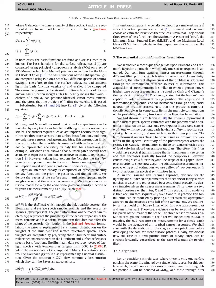
544 In short, the active Bayesian formulation is, in fact, sequential,545 where the posterior for each image acts as a prior for the next im-546 age, and the posterior for each filter portion acts as a prior for the547 next filter portion. This is similar to the sequential nature of the548 ‘‘Static Camera” case (in Section 3.2.1), where the posterior for each549 surface patch acts as a prior for the next surface patch. The addition550 of more surface patches in the scene provides more information551 regarding the illumination and thus, in turn, about the surface552 patch spectra themselves. In addition, moving the camera provides553 more information about the scene as the surface patches are554 viewed from different locations with respect to the filter, and thus555 many images of the same scene are obtained. This allows for556 acquiring multiple measurements for the same surface patch and557 thus improves on parameter estimation.

558 3.3. Generalization: two to multiple portion filters

559 We illustrated the sequential nature of the proposed active560 Bayesian formulation for the case of two portion filters. As shown561 above, the posterior for each filter portion acts as a prior for the562 next filter portion. This hypothesis can be generalized to the case563 of more than two portion filters in the scene. Consider, for exam-564 ple, the ‘‘Static Camera” case when there is a filter of three por-565 tions, taken in the order X;Y ; Z, and when there are three-surface566 patches in the scene. The scene in this example looks similar to567 that in Fig. 1 except that patch 2 is viewed through filter portion568 Y and Z instead of only filter portion Y. Patches 1 and 3 are viewed569 through filter portions X and Y as in Fig. 1. Call P3 the conditional570 posterior function for all three portions of the multiple filter for571 the parameters of the surfaces and the light source given the set572 of measurements of the scene. P3 would be a function of the pos-573 terior for the first two portions X and Y of the filter, (call it P2),574 the likelihood of the measurements taken through the third por-575 tion of the filter ðZÞ, and the prior of the spectral function weights576 of the surface patches viewed through only portion Z of the filter577 (none in this case):

P3 ¼ P2pðRGBZ2ja2; bÞ: ð27Þ579579

580 In turn, P2 would be a function of the posterior for the first filter581 portion ðXÞ, the likelihood of the measurements taken through the582 second filter portion ðYÞ, and the prior of the spectral function583 weights viewed through only filter portion Y:

P2 ¼ P1pðRGBY1ja1; bÞpðRGBY2ja2; bÞpðRGBY3ja3; bÞpða2Þ: ð28Þ585585

586Therefore the derivation of the posterior can be straight-forwardly587extended from incorporating measurements taken through two fil-588ter portions to incorporating measurements taken through three fil-589ter portions. This extension can also be applied to the ‘‘Moving590Camera” case (Section 3.2.2).

5914. Experiments

592The main purpose of the experiments performed is to show593that, despite the assumptions imposed, additional measurements594obtained for a patch viewed through a filter do improve surface595and illuminant spectral estimates. Constructing a filter with multi-596ple portions of different spectral sensitivities is beyond the scope of597this work as explained in Section 3. Therefore we choose to illus-598trate the performance of the approach for the case of two portion599filters. Note that we had shown in simulation in [20] that improve-600ment in spectral estimation can be obtained with the introduction601of filters with more than two portions into the scene as well.602In this work, we refer to a measurement system with two por-603tions, transparent and filtered, as a binary filter. The optical filter604chosen for the filtered portion should be such that there are signif-605icant differences between the responses from the transparent por-606tion and the filtered portion in the long-, medium-, and short-607wavelength range channels. In addition, the filter should not com-608pletely block the light from the wavelengths that a given photore-609ceptor is sensitive to. For example, a ‘‘brick-wall” yellow optical610filter should not be employed, as it would completely block the611portion of the spectrum responded to by the short-wavelength612channel while passing through unchanged the portions of the spec-613trum responded to by the long- and medium-wavelength channels.614Taking into account these issues, we choose to use an Edmund Op-615tics BG 18 bandpass filter of spectral transmittance peaking in the616blue-green wavelength region. This filter shifts the spectral sensi-617tivity of the long- and short-wavelength sensors towards medium618wavelengths, and narrows the bandwidth of the medium-wave-619length sensor. Thus, it is expected that the binary filter measure-620ment system should provide better spectral modeling at medium621wavelengths than the non-filter measurement system.622Before moving on to describing the implementation and testing623specifics of the algorithm and the results obtained, we would like624to note that some previous color constancy approaches investi-625gated the idea of using multiple measurements for the same sur-626face. For example, Tsukada and Ohta [21], who employed linear627model representations for surface and illuminant spectra, used628two illuminants to capture two images of the same scene. While

Fig. 2. Moving camera. Three patches in the scene, illuminated by a single light source viewed by a sensor through a two portion or binary filter, which has one transparent

part and one part tinted blue-green (represented with the hashed part), for example. The camera is moved twice. a1; a2; a3 and b are the weights in the spectral linear models

for patches 1, 2, 3 and the illuminant, respectively. (For interpretation of the references to colours in this figure legend, the reader is referred to the web version of this paper.)






UNCORRECTEDPROOF

629 their approach may seem similar to the proposed one, the authors630 in [21] employed more unknowns as the number of basis function631 illuminant spectra is doubled with the use of two illuminants. Also,632 D’Zmura and Iverson [13,14,22] studied the case where multiple633 light sources were used to capture multiple images of the same634 scene. However their approach suffers from many limitations as635 is discussed in Section 2.636 Within the color correction approaches that use 3D color space637 representations such as RGB, it has been shown how illumination638 variation in an image can be used as an additional constraint to im-639 prove on color constancy [23,24]. Finlayson et al. introduced the640 Chromagenic color constancy approach [25,26], where a filtered641 and a non-filtered image are obtained for each scene. As mentioned642 in [25], the additional measurements are not used to increment the643 number of knowns to facilitate the estimation of the model param-644 eters as is the case in the proposed algorithm. These measurements645 are used to compute the relationship between the filtered and non-646 filtered RGB’s. This relationship is used to select the scene illumi-647 nant, and given the illuminant, color correction can be performed.648 The Chromagenic color constancy approach is described for the649 case of using two measurements for each surface. However, in650 the case of three or more measurements per surface, the calcula-651 tions can become tedious, and it would be more difficult to com-652 pute the relationship between the non-filtered and the filtered653 RGB’s at once. On the other hand, the proposed spectral based ap-654 proach can handle the incorporation of additional measurements655 in a more natural and inexpensive way using Bayesian techniques656 as described in the previous section. Moreover, our approach al-657 lows for flexibility in the sense that if only non-filtered RGB mea-658 surements are available for some surface patches, these can still659 be used in the posterior distribution. This is not the case in Chro-660 magenic color constancy, where each surface patch should have661 two sets of measurements in order for the formulation of the prob-662 lem to be complete.

663 4.1. Experimental setup

664 We captured images of the pages in the Munsell Book of Color665 [18] with a Panasonic WV-CP410 camera. All the images were ob-666 tained in our laboratory at night to ensure that the only illumina-667 tion was that of the scene light source. We obtained a 50 � 50 pixel668 sample from each of the Munsell patches using a semi-automated669 segmentation algorithm. Since we assume Mondrian scenes where670 the illumination is locally constant, we averaged the RGB responses671 of all the pixels in a segmented patch to obtain one RGB response672 per patch. The same steps were carried out in the case of the fil-673 tered portion of the camera lens to obtain RGB responses for the674 patches viewed through a filter. Since we assume flat scenes where675 there are no interreflections, the average responses corresponding676 to the patches in the scene, in the filter and no filter cases, were677 inputted into our algorithm.678 We start by explaining how the scenes were constructed. Ten679 surface patches, which we shall refer to as main patches, were cho-680 sen at random. Ten groups of two patches each were then selected681 randomly, and these groups were used to construct 10 three-sur-682 face patch scenes with the main patch repeated in all 10 scenes.683 Since there were 10 main patches, a total of 100 scenes was con-684 structed. The selection of scenes was done in this fashion so as to685 allow more robust evaluation of spectral estimation for the main686 patch which is repeated in 10 scenes. All the constructed scenes687 comprised of three randomly chosen matte Munsell surface688 patches [18] illuminated by a single 60W tungsten light source689 at temperature 2800 K. The spectra of these patches were mea-690 sured by Parkkinen and Silfsten [27]. The database of light source691 spectra comprised of a set of tungsten light spectra at tempera-692 tures ranging from 2600 to 3500 K, in steps of 100 K, and was ob-

693tained from the IES lighting handbook [28]. The spectral694sensitivities of the camera sensor were obtained from the manu-695facturer. The wavelengths considered are over the visible range,696430–700 nm, which is discretized into 5 nm intervals. Note that697the choice of surface and illuminant spectral databases would698not make a difference in the performance of the approach as the699basis functions can be updated accordingly to be the principal700components of the new spectral databases. The performance of701the approach, however, depends on how well the basis functions702represent the spectral databases for each of the surfaces and the703light source.704For the Bayesian formulations, the likelihood functions705pðfRGBgja1; a2; a3; bÞ are computed using the sensor measurements706as well as the corresponding model predictions, which are given in707Eq. (5). We describe what the sensor measurements are for each708case studied in the next section. The standard deviation of the like-709lihood is an approximation of the standard deviation of the mea-710surement noise. The latter standard deviation is computed by711capturing 50 snapshots of each of the Munsell patches with a712100 ms delay between snapshots. Then, the standard deviation of713the noise corresponding to each patch sensor response is calcu-714lated using the 50 snapshots of the patch. Finally, the standard715deviations of the sensor response noise of all the patches is aver-716aged to obtain the likelihood standard deviation. While this may717be an oversimplified way of computing the standard deviation, it718serves the purpose and can be reproduced fairly easily upon chang-719ing the database of surface patches. Note that the same standard720deviation as computed above is used when modeling the likelihood721in the case of a filter. This means that it is assumed that the stan-722dard deviation of the noise is approximately the same in this case.723This assumption is made for simplification purposes as it avoids724the need of estimating standard deviations for different filters.725The illuminant spectrum EðkÞ is modeled with five basis functions,726while the surface spectrum SxðkÞ is modeled with eight basis func-727tions. The weights for these spectra are assumed to have Gaussian728distributions. The basis functions for the surface spectrum model729are represented by the principal components of the spectra of730the 1269 Munsell patches provided by Parkkinen and Silfsten731[27]. The basis functions for the light source spectrum model are732represented by the principal components of the spectra of the 10733tungsten light spectra [28].734The prior distributions for the spectral model parameters735pða1; a2; a3; bÞ are assumed to be independent and are modeled by736Gaussian distributions. The means and variances of the prior func-737tions are computed from the distribution of weights corresponding738to the 1269 Munsell patch spectra and the 10 tungsten light spec-739tra used. These weights are obtained by projecting the measured740spectra onto the basis function sets.741The location of the mode of the posterior distribution is esti-742mated by a standard MATLAB optimization package, lsqnonlin,743resulting in a set of estimated surface and light source spectra744weight vectors. Note that any package can be used provided that745the negative of the cost function can be minimized. In order to746eliminate the chances of obtaining a set of weights corresponding747to a local minimum, the optimization is run with 10 different ran-748domly chosen starting points. In most cases, the optimization ter-749minates at the same cost function value. In the occasional cases750when it does not, we choose the solution weight vector corre-751sponding to the smallest value.

7524.2. Experimental results

753First, we compare the spectral estimates obtained in the binary754filter case to those obtained in the no filter case, which is equiva-755lent to Brainard and Freeman’s approach. Next, we show howmov-756ing the camera, once and then twice, to acquire additional






UNCORRECTEDPROOF

757 measurements for a surface patch improves spectral estimation.758 Experiments with three-surface patches in the scene, illuminated759 by a single light source (as described in Section 3) are performed.760 The resulting estimates for the model and the actual spectra for761 the surface patches and the light sources are plotted and the root762 mean square (RMS) errors are computed in each of the two cases763 below. We would like to note that, to the best of our knowledge,764 this is the first time that Brainard and Freeman’s approach is ap-765 plied on real data.

766 4.2.1. Static camera767 We compare the performance of the approach in the no filter768 case to that of the binary filter case. In the no filter case, one RGB769 response is obtained for each surface patch in the scene. In the bin-770 ary filter case, two RGB responses corresponding to the different771 portions of the filter are obtained for each of surface patches 1772 and 3. One RGB response corresponding to filter portion Y is ob-773 tained for surface patch 2 (see Fig. 1). These sensor responses are774 used in computing the likelihood functions, which in turn are used775 in the computation of the posteriors as described in Section 3.2.1.776 The resulting estimates for the model and the actual spectra for the777 tungsten light source and a surface patch from one of the scenes778 can be found in Fig. 3. Note that RMS error is indicated as RMSE779 in the corresponding plots. The plots show that the model spectra780 are closer to the actual spectra in the binary filter case than in the781 no filter case.782 Moreover, we depict in Fig. 4 the average over 10 scenes of the783 RMS errors between the model and actual spectra for the illumi-784 nant and the main surface patches, which are repeated in a set of

78510 scenes. We also depict the average of all the average RMS errors786in the last two bars for each plot. AVE denotes this average. From787these plots we observe that there is always an improvement in788the illuminant spectral estimates. Theoretically, this should lead789to an improvement in the surface spectral estimates. Despite the790fact that this is not always the case as we can see in Fig. 4b, there791is either no improvement or an improvement in 50% of the cases.792To get a better understanding of the comparative performance793of the approach in the no filter and filter cases, the paired T-test794[29] is run on the average RMS errors for the 10 scene sets (de-795picted in Fig. 4) for a 95% confidence level. Note that this test as-796sumes that the differences between the average RMS errors have797a normal distribution. As a result of the test, the improvement in798performance for the binary filter case over the no filter case for799the illuminant spectral estimates is statistically significant800ðt ¼ 4:848; p < 0:05Þ. As for the surface spectral estimates, the dif-801ference in performance between the no filter and the binary filter802case is not statistically significant ðt ¼ �0:639; p < 0:05Þ. There-803fore we cannot conclude from the latter results that the average804performance for the no filter case is better than that for the binary805filter case as implied by the last two bars in Fig. 4b.

8064.2.2. Moving camera807We show results for the moving camera case, as described in808Section 3.2.2. There are three-surface patches in the scene with a809filter of two portions, represented by a binary filter on the lens hav-810ing a transparent part and a tinted blue–green part. The camera is811moved: once and then twice. Before moving the camera, the sensor812responses obtained are two for surface patch 1, corresponding to

450 500 550 600 650 7000

0.2

0.4

0.6

0.8

1

Wavelength nm

Norm

aliz

ed R

adia

nt P

ow

er

actual

model,no filter

model,filter

450 500 550 600 650 7000

0.2

0.4

0.6

0.8

1

Wavelength nm

Norm

aliz

ed S

pectr

al R

eflecta

nce

actual

model,no filter

model,filter

Fig. 3. The estimated and actual spectra when there are multiple surface patches in the scene in the cases of no filter and binary filter for each of the (a) tungsten illuminant at

2800 K, RMSE = 0.0930 (no filter), RMSE = 0.0533 (filter) and (b) Munsell patch 1203, RMSE = 0.1705 (no filter), RMSE = 0.1282 (filter).

0

0.02

0.04

0.06

0.08

0.1

0.12

0.14

Avera

ge R

MS

err

or

Scene Set Number

1 2 3 4 5 6 7 8 9 10AVE

no filter

filter

0

0.05

0.1

0.15

0.2

Avera

ge R

MS

err

or

Surface Patch Number

451

686

328

747 63 71

487

612

03 938

925

AVE

no filter

filter

Fig. 4. Average RMS errors for the illuminant and 10 surface patch spectra for the no filter and binary filter cases when there are multiple surface patches in the scene. Each

error is the average RMS error over 10 scenes chosen at random for the spectrum of the (a) tungsten illuminant at 2800 K and (b) repeated Munsell patch in each 10 scenes.






UNCORRECTEDPROOF

813 each of the filter portions X and Y, and one for each of surface814 patches 2 and 3, corresponding to filter portion Y. The sensor re-815 sponses obtained after the camera is moved the first time are the816 same as the previous ones, with an additional sensor response ob-817 tained for surface patch 2 corresponding to filter portion Y (see818 Fig. 2). The sensor responses obtained after the camera is moved819 the second time are the same as the previous ones, with an addi-820 tional sensor response obtained for surface patch 3 corresponding821 to filter portion Y. These sensor responses are used in computing822 the likelihood functions corresponding to each of the one move823 and two moves cases. The posterior functions are then computed824 as described in Section 3.2.2. The hypothesis is that the estimates825 will improve with each move for the patches for which additional826 measurements are obtained upon moving. Fig. 5 shows the model827 and the actual spectra as well as the RMS errors for both the light828 source and one of the three-surface patches in a scene respectively.829 Notice how the RMS errors in this figure are reduced by moving.830 Moreover, we depict the average over 10 scenes of the RMS er-831 rors between the model and actual spectra for the illuminant and832 the main surface patches, which are repeated in a set of 10 scenes833 as seen in Fig. 6. We also depict the average of all the average RMS834 errors in the last three bars for each plot. We can see that the aver-835 age RMS errors are reduced with every camera move for the illumi-836 nant. This should imply decreasing RMS errors with every move for837 the surface patches as well, which is evident in 80% of the cases.838 To get a better understanding of the comparative performance839 of the approach in the no move, one move, and two moves cases,

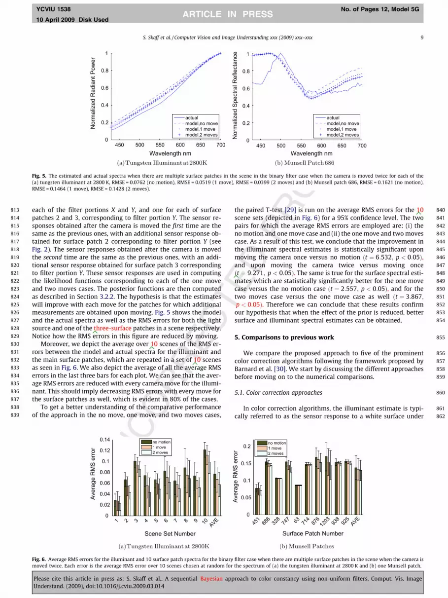
840the paired T-test [29] is run on the average RMS errors for the 10841scene sets (depicted in Fig. 6) for a 95% confidence level. The two842pairs for which the average RMS errors are employed are: (i) the843nomotion and one move case and (ii) the one move and twomoves844case. As a result of this test, we conclude that the improvement in845the illuminant spectral estimates is statistically significant upon846moving the camera once versus no motion ðt ¼ 6:532; p < 0:05Þ,847and upon moving the camera twice versus moving once848ðt ¼ 9:271; p < 0:05Þ. The same is true for the surface spectral esti-849mates which are statistically significantly better for the one move850case versus the no motion case ðt ¼ 2:557; p < 0:05Þ, and for the851two moves case versus the one move case as well ðt ¼ 3:867;852p < 0:05Þ. Therefore we can conclude that these results confirm853our hypothesis that when the effect of the prior is reduced, better854surface and illuminant spectral estimates can be obtained.

8555. Comparisons to previous work

856We compare the proposed approach to five of the prominent857color correction algorithms following the framework proposed by858Barnard et al. [30]. We start by discussing the different approaches859before moving on to the numerical comparisons.

8605.1. Color correction approaches

861In color correction algorithms, the illuminant estimate is typi-862cally referred to as the sensor response to a white surface under

450 500 550 600 650 7000

0.2

0.4

0.6

0.8

1

Wavelength nm

Norm

aliz

ed R

adia

nt P

ow

er

actual

model,no move

model,1 move

model,2 moves

450 500 550 600 650 7000

0.2

0.4

0.6

0.8

1

Wavelength nm

Norm

aliz

ed S

pectr

al R

eflecta

nce

actual

model,no move

model,1 move

model,2 moves

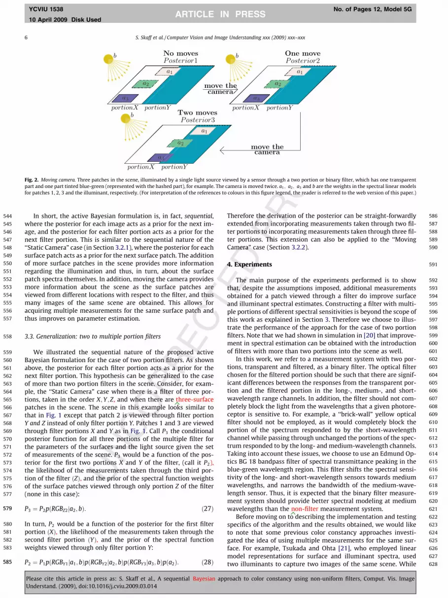
Fig. 5. The estimated and actual spectra when there are multiple surface patches in the scene in the binary filter case when the camera is moved twice for each of the

(a) tungsten illuminant at 2800 K, RMSE = 0.0762 (no motion), RMSE = 0.0519 (1 move), RMSE = 0.0399 (2 moves) and (b) Munsell patch 686, RMSE = 0.1621 (no motion),

RMSE = 0.1464 (1 move), RMSE = 0.1428 (2 moves).

0

0.02

0.04

0.06

0.08

0.1

0.12

0.14

Avera

ge R

MS

err

or

Scene Set Number

1 2 3 4 5 6 7 8 9 10AVE

no motion

1 move

2 moves

0

0.05

0.1

0.15

0.2

Avera

ge R

MS

err

or

Surface Patch Number

451

686

328

747 63 71

487

612

03 938

925

AVE

no motion

1 move

2 moves

Fig. 6. Average RMS errors for the illuminant and 10 surface patch spectra for the binary filter case when there are multiple surface patches in the scene when the camera is

moved twice. Each error is the average RMS error over 10 scenes chosen at random for the spectrum of (a) the tungsten illuminant at 2800 K and (b) one Munsell patch.






UNCORRECTEDPROOF

863 a canonical illuminant. The canonical illuminant is the one selected864 from the database of illuminant spectra for which the camera is865 most balanced. The first algorithm is the Gray World, GW [7]. It as-866 sumes that the scene average is identical to the camera response to867 a chosen gray surface under the canonical illuminant. The illumi-868 nant RGB, which is equivalent to the camera response to a white869 surface, is taken to be double the response to a gray surface, again870 under the canonical illuminant. The second algorithm, Scale-by-871 Max, takes the illuminant RGB estimate to be the maximum in each872 channel (red, green, blue) over all the camera responses to all the873 surfaces in a scene [31]. The third algorithm is Color by Correlation874 proposed by Finlayson et al. [32,33] as an improvement to the Col-875 or in Perspective algorithm [34]. In the Color by Correlation algo-876 rithm, a correlation matrix in which each column corresponds to877 a different training illuminant and each row corresponds to a dif-878 ferent image chromaticity is built. The chromaticities are com-879 puted from the surface reflectances in the training set. The880 convex hull of the chromaticities corresponding to one illuminant881 is computed. All the entries of the chromaticity bins falling in the882 convex hull are set to one, while all other elements are set to zero.883 The correlation matrix is multiplied by a vector containing infor-884 mation about the image chromaticities. This vector has the same885 discretization as the rows in the correlation matrix. An entry of this886 vector is set to one if the chromaticity occurs in the image and to887 zero otherwise. The scene illuminant selected is the one corre-888 sponding to the maximum correlation between the correlation889 matrix and the vector of chromaticities. This algorithm is labeled890 as C-by-C-01.891 The last two algorithms which we compare our approach to are892 based on Forsyth’s gamut mapping approach [35], which generally893 comprises two steps. The first step is to form two convex sets of894 RGB’s represented by their respective convex hulls. One set com-895 prises all possible surface RGB’s when illuminated under a canoni-896 cal illuminant. The other set comprises all surface RGB’s under the897 unknown illuminant, and therefore the convex hull is the set of ob-898 served RGB’s in this case. The two hulls are a unique diagonal map-899 ping of each other under the diagonal assumption of illumination900 change. The set of possible maps is computed and the solution901 diagonal map is sought. This map corresponds to the solution set,902 which corresponds to the set of the surface RGB’s under the canon-903 ical illuminant. This is the second step of the algorithm. Finlayson904 added two ideas to Forsyth’s approach to introduce the Color in905 Perspective (CIP) approach [34]. First, he showed how to perform906 gamut mapping in 2D (chromaticity) instead of 3D ðRGBÞ space907 as this simplifies gamut mapping and renders it usable in the real908 world, where specularities and varying illumination are com-909 monly-arising problems. Second, he suggested that the diagonal910 maps can be restricted to only those corresponding to expected911 illuminants. As the illumination constraint is non-convex, Barnard912 [36] introduced the assumption of the convex hull for this con-913 straint (ECRULE). As for obtaining the solution set, which is the sec-914 ond step of a gamut mapping algorithm, there are three methods.915 The first one is choosing the solution set with the maximum vol-916 ume [34,35]. The second one is taking the average of the constraint917 set [36]. The third one is averaging over the non-convex constraint918 set using Monte Carlo integration [37]. Following Barnard et al.’s919 framework [30], here the solution is selected by taking the center920 of mass of the constraint set, referred to as ICA (Illumination Con-921 strained Average).

922 5.2. Numerical results

923 Our goal is to compare our approach to the algorithms dis-924 cussed in the previous section. This implies that the chosen data925 sets and priors needed for these algorithms are chosen in ways that926 yield them comparable to the method proposed in this paper. First,

927the scenes used for testing are the same as the ones used in the928previous section. They therefore consist of three-surface patches929illuminated by a single light source. Second, the database of light930source spectra used for training in the Color by Correlation ap-931proach is the same as that used for computing the prior functions932in our approach. This is a set of tungsten light spectra at tempera-933tures ranging from 2600 to 3500 K, in steps of 100 K. Next, the934canonical illuminant selected from this set is such that the camera935is most balanced, and is therefore tungsten light at 3500 K. Note936that the canonical illuminant choice can be arbitrary according to937Barnard et al. [30]. In addition, the set of RGB measurements used938to obtain the convex hull in the 2D and 3D Gamut Mapping ap-939proaches are the camera sensor responses of all 1269 patches from940the Munsell Book of Color [18]. In addition, the reflectance spectra941of these patches are used in the Gray World approach. All the spec-942tra employed in the previous approaches are 55D and over the943same wavelength range as in our approach.944The approach proposed in this paper estimates both illuminant945and surface spectra. However, the described algorithms perform946color correction after carrying out an illumination estimation step.947Therefore, we focus on comparing the performance of illuminant948estimation of the different algorithms. Since we are interested in949the chromaticity of the illuminant, we choose the second error950measure in Barnard’s framework [30] for comparison. To obtain951this error measure, the chromaticities for each of the actual and952model illuminants given their RGB’s is computed:

ðra; gaÞ ¼ ðRa=ðRa þ Ga þ BaÞ;Ga=ðRa þ Ga þ BaÞÞ;

ðrm; gmÞ ¼ ðRm=ðRm þ Gm þ BmÞ;Gm=ðRm þ Gm þ BmÞÞ;ð29Þ

954954

955where ðRa;Ga;BaÞ is the RGB of the actual illuminant and ðRm;Gm;BmÞ

956is the RGB of the model illuminant. The error E is the vector distance957between the two chromaticities:

E ¼

ffiffiffiffiffiffiffiffiffiffiffiffiffiffiffiffiffiffiffiffiffiffiffiffiffiffiffiffiffiffiffiffiffiffiffiffiffiffiffiffiffiffiffiffiffiffiffiffiffi

ðrm � raÞ2 þ ðgm � gaÞ

2q

: ð30Þ 959959

960Our approach estimates an illuminant spectral model, which is pro-961jected onto the three sensitivity curves of the camera sensor to ob-962tain the equivalent three-dimensional RGB measurement. From this963RGB, the corresponding chromaticity coordinates and then E are964computed for each scene. The median RMS error is computed to965measure the performance of the approach in estimating illuminant966spectra for all 100 scenes [38].967Next, the median RMS error is computed for the illuminant968chromaticity estimate of the same 100 scenes as given by the five969previous algorithms. These errors are shown in Table 1. As there970are many variants for each of the Color by Correlation, 2D Gamut971Mapping, and 3D Gamut Mapping algorithms, the variant which

Table 1

The median RMS errors for the illuminant estimates of 100 scenes (except for 2D

Gamut Mapping) given by five previous approaches, Brainard and Freeman’s

approach, and the different variants of the proposed approach. For the scene setup

in the case of Sequential Bayesian – Binary Filter, Static Camera, see Fig. 1. For the

scene setup in the case of Sequential Bayesian – Binary Filter: No moves, One move,

and Two moves, see Fig. 2. N denotes the number of gathered sensor responses or

measurements.

Algorithm Median RMS error

Gray World 0.2528

Scale-by-Max 0.2520

C-by-C-01 0.0366

2D Gamut Mapping (CIP) – ICA 0.0619

3D Gamut Mapping (ECRULE) – ICA 0.0698

Brainard–Freeman N ¼ 3 0.0454

Sequential Bayesian – Binary Filter, No Moves N ¼ 4 0.0427

Sequential Bayesian – Binary Filter, One Move N ¼ 5 0.0355

Sequential Bayesian – Binary Filter, Static Camera N ¼ 5 0.0350

Sequential Bayesian – Binary Filter, Two Moves N ¼ 6 0.0310






UNCORRECTEDPROOF

972 gives rise to the minimal median RMS error over the 100 illumi-973 nants is selected. In addition, the median RMS errors of Brainard974 and Freeman’s approach as well as the different variants of our ap-975 proach are shown in the table in decreasing order. As expected, the976 order of median RMS errors corresponds to an increasing number977 of sensor measurements (denoted by N in the table) in each of978 the scenarios. However, in the Sequential Bayesian – Binary Filter,979 One Move and the Sequential Bayesian – Binary Filter, Static Cam-980 era cases, the number of gathered RGB measurements is the same981 (N ¼ 5). This reflects in the very small difference in the correspond-982 ing median RMS errors.983 First, we would like to note that the 2D Gamut Mapping algo-984 rithm did not find a solution for 28 out of the 100 scenes. This985 may be due to the fact that the canonical gamut, formed by the986 RGB’s of the surfaces viewed under the canonical illuminant, is lim-987 ited as it does not take into account all possible surfaces. Only the988 surface patches from our data set are considered. The median RMS989 error given in the table for 2D Gamut Mapping is, therefore, over990 72 scenes. From the table, it can be concluded that the Gray World991 and the Scale-by-Max algorithms perform poorly as expected since992 the assumptions imposed by these algorithms are strong and are993 not always valid for real world images. The Color by Correlation994 algorithm performs relatively well compared to the other four pre-995 vious approaches as it does not impose as strong a set of assump-996 tions. This explains its low median RMS error. Finally, we conclude997 that the proposed Sequential Bayesian approach yields the best998 illuminant spectral estimates when at least five sensor measure-999 ments are employed when there are three-surface patches in the

1000 scene, as in the Binary Filter – Static Camera, the Binary Filter –1001 One Move, and the Binary Filter – Two Moves cases. Our approach1002 has an advantage over the gamut mapping approaches in that it1003 does not require a canonical gamut, which should be formed by1004 taking into account as many surface patches as possible. Moreover,1005 our approach does not impose any assumptions on the scene under1006 study, which is the case in the Gray World and Scale-by-Max algo-1007 rithms. Therefore, our approach demonstrates flexibility of use.

1008 6. Conclusions

1009 In this work, we have proposed a sequential Bayesian strategy1010 that builds on the Brainard–Freeman Bayesian approach to color1011 constancy [1]. The recursion helps in gathering information across1012 different scenes and filter portions of different spectral sensitivi-1013 ties. Brainard and Freeman used a Bayesian technique to regularize1014 the problem of computing the values of the illuminant and surface1015 reflectance spectra parameters [39]. This technique uses the bilin-1016 ear model of Maloney and Wandell [10] to provide a parametriza-1017 tion of the illuminant and surface patch spectra.1018 Our approach enhances Brainard and Freeman’s model and is1019 based on insight from the characteristics of human vision, and1020 the human eye, in particular. In our approach, measurements are1021 acquired sequentially from each portion of a filter, similar to when1022 a person moves his/her gaze across a surface in the scene. In this1023 paper we modeled the case of a non-uniform filter, which has1024 two portions of different spectral sensitivities. We also extended1025 this case to moving the camera across the scene.1026 The experimental results in Section 4 indicate that there is con-1027 siderable improvement in the illuminant spectra estimates with1028 the introduction of the binary filter method compared to the no fil-1029 ter method, which is equivalent to that of Brainard and Freeman.1030 Another result shown in Section 4 is that of the moving camera:1031 the more the number of moves of the camera, the more measure-1032 ments for surface patches obtained. This motion results in an1033 improvement in the estimates of the illuminant and surface spec-1034 tra. Next, the numerical comparisons of illuminant estimation in

1035Section 5 show that the proposed algorithm, in the case of a certain1036number of gathered sensor responses from a scene, can outperform1037state-of-the-art color correction approaches.1038In our work, we rely heavily on the Bayesian probabilistic for-1039mulation. We believe that this formulation is a suitable approach1040because it models the uncertainties in all parts of a system, on1041one hand, and because it employs spectral models, on the other1042hand. Spectral models make it easier to further extend this Bayes-1043ian approach to incorporate measurements from different scenes.1044In addition, spectral models as used in our approach do not require1045all surface patches of the scene to be viewed under all portions of a1046filter. Finally, the computational complexity of the Bayesian formu-1047lation is tolerable, which makes it feasible to implement and run1048our sequential formulation.

1049Acknowledgements

1050Wewould like to thank Kobus Barnard for making his code pub-1051licly available. This research was funded by a grant from the Cana-1052dian Natural Sciences and Engineering Research Council (NSERC).

1053References

1054[1] D.H. Brainard, W.T. Freeman, Bayesian color constancy, Journal of the Optical1055Society of America A 32 (7) (1997) 1393–1411.1056[2] J.J. Clark, J.K. O’Regan, A temporal difference learning model for perceptual1057stability in color vision, in: IEEE International Conference on Pattern1058Recognition, Barcelona, Spain, 2000, pp. 503–506.1059[3] J.J. McCann, S.P. McKee, T.H. Taylor, Quantitative studies in retinex theory – a1060comparison between theoretical predictions and observer responses to the1061‘color mondrian’ experiments, Vision Research 16 (5) (1976) 445–448.1062[4] K. Barnard, L. Martin, A. Coath, B. Funt, A comparison of computational color1063constancy algorithms. II. Experiments with image data, IEEE Transactions on1064Image Processing 11 (9) (2002) 985–996.1065[5] M. Brill, G. West, Contributions to the theory of invariance of colour under the1066condition of varying illumination, Journal of Mathematical Biology 11 (3)1067(1981) 337–350.1068[6] J.v. Kries, Beitrag zur physiologie der gesichtsempfinding, Arch. Anat. Physiol. 21069(1878) 5050–5524 Q1.1070[7] G. Buchsbaum, A spatial processor model for object colour perception, Journal1071of the Franklin Institute 310 (1980) 1–26.1072[8] R. Gershon, A.D. Jepson, J.K. Tsotsos, From [r, g, b] to surface reflectance:1073computing color constant descriptors in images, in: International Joint1074Conference on Artifical Intelligence, 1987, pp. 755–758.1075[9] L.T. Maloney, Computational approaches to color constancy, Ph.D. Thesis,1076Stanford University, Stanford, CA, 1985.1077[10] L.T. Maloney, B.A. Wandell, Color constancy: a method for recovering surface1078spectral reflectance, Journal of the Optical Society of America A 3 (1) (1986)107929–33.1080[11] A. Yuille, A method for computing spectral reflectance, Biological Cybernetics108156 (1987) 195–201.1082[12] M.D. D’Zmura, P. Lennie, Mechanisms of color constancy, Optical Society of1083America A 10 (3) (1986) 1662–1672.1084[13] M.D. D’Zmura, G. Iverson, Color constancy I. Basic theory of two-stage linear1085recovery of spectral descriptions for lights and surfaces, Journal of the Optical1086Society of America A 10 (10) (1993) 2148–2165.1087[14] M.D. D’Zmura, G. Iverson, Color constancy II. Results for two-stage linear1088recovery of spectral descriptions for lights and surfaces, Journal of the Optical1089Society of America A 10 (10) (1993) 2166–2180.1090[15] J. Ho, B.V. Funt, M.S. Drew, Separating a color signal into illumination and1091surface reflectance components: theory and applications, IEEE Transactions on1092Pattern Analysis and Machine Intelligence 12 (10) (1990) 966–977.1093[16] T.O. Berger, Statistical Decision Theory and Bayesian Analysis, Springer, New1094York, NY, 1985.1095[17] R.O. Duda, P.E. Hart, Pattern Classification and Scene Analysis, Wiley, Stanford,1096CA, 1973.1097[18] Munsell Book of Color-Matte Finish Collection, Munsell Color, Baltimore, MD,10981976.1099[19] J.P.S. Parkkinen, J. Hallikainen, T. Jaaskelainen, Characteristic spectra of Munsell1100colors, Journal of the Optical Society of America A 6 (2) (1989) 318–322.1101[20] S. Skaff, T. Arbel, J.J. Clark, Active Bayesian color constancy with non-uniform1102sensors, in: IEEE International Conference on Pattern Recognition, vol. 2,1103Quebec City, QC, 2002, pp. 681–684.1104[21] M. Tsukada, Y. Ohta, An approach to color constancy using multiple images, in:1105Proceedings of the 3rd IEEE International Conference on Computer Vision,1106Osaka, Japan, 1990, pp. 385–389.1107[22] M.D. D’Zmura, G. Iverson, Color constancy III. General linear recovery of1108spectral descriptions for lights and surfaces, Journal of the Optical Society of1109America A 11 (9) (1994) 2389–2400.






UNCORRECTEDPROOF

1110 [23] G.D. Finlayson, B.V. Funt, K. Barnard, Color constancy under varying1111 illumination, in: IEEE International Conference on Computer Vision,1112 Cambridge, MA, 1995, pp. 720–725.1113 [24] K. Barnard, G. Finlayson, B. Funt, Color constancy for scenes with varying1114 illumination, Computer Vision and Image Understanding 65 (2) (1997) 311–321.1115 [25] G.D. Finlayson, S.D. Hordley, P. Morovic, Colour constancy using the1116 chromagenic constraint, in: IEEE Conference on Computer Vision and Pattern1117 Recognition, vol. 1, 2005, pp. 1079–1086.1118 [26] G.D. Finlayson, P.M. Morovic, S.D. Hordley, Chromagenic colour constancy, in:1119 Proceedings of the 10th Congress of the International Colour Association, 2005.1120 [27] J.P. Parkkinen, P. Silfsten, Database of spectra, University of Joensuu, Finland,1121 Available from: <http://spectral.joensuu.fi/index.php?page=database&info=1122 munsell_matt/>.1123 [28] I.E.S. of North America, IES lighting handbook, Illuminating Engineering1124 Society of North America, New York, NY, 1981.1125 [29] D.J. Sheskin, Handbook of Parametric and Nonparametric Statistical1126 Procedures, Chapman & Hall/CRC Press, New York, NY, 2000.1127 [30] K. Barnard, V. Cardei, B. Funt, A comparison of computational color constancy1128 algorithms. I. Methodology and experiments with synthesized data, IEEE1129 Transactions on Image Processing 11 (9) (2002) 972–984.

1130[31] E.H. Land, The retinex theory of color vision, Scientific American 237 (6) (1977)1131108–128.1132[32] G.D. Finlayson, P.M. Hubel, S. Hordley, Color by correlation, in: Proceedings of1133the Fifth Color Imaging Conference, 1997, pp. 6–11.1134[33] G.D. Finlayson, S.D. Hordley, P.M. Hubel, Color by correlation: a simple1135unifying framework for color constancy, IEEE Transactions on Pattern Analysis1136and Machine Intelligence 23 (11) (2001) 1209–1221.1137[34] G.D. Finlayson, Color in perspective, IEEE Transactions on Pattern Analysis and1138Machine Intelligence 18 (10) (1996) 1034–1038.1139[35] D.A. Forsyth, A novel algorithm for color constancy, International Journal of1140Computer Vision 5 (1) (1990) 5–36.1141[36] K. Barnard, Computational colour constancy: taking theory into practice,1142Master’s Thesis, Simon Fraser University, School of Computing (August 1995).1143[37] G. Finlayson, S. Hordley, Selection for gamut mapping colour constancy, Image1144and Vision Computing 17 (8) (1999) 597–604.1145[38] S.D. Hordley, G.D. Finlayson, Reevaluation of color constancy algorithm1146performance, Journal of the Optical Society of America A 23 (5) (2006)11471008–1020.1148[39] A.N. Tikhonov, V.Y. Arsenin, Solutions of Ill-Posed Problems, V.H. Winston,1149Washington, DC, 1977.

1150






http://spectral.joensuu.fi/index.php?page=database&info=munsell_matt

http://spectral.joensuu.fi/index.php?page=database&info=munsell_matt

Documents

A sequential Bayesian approach to color constancy using non-uniform filters