A STUDY OF THE PRESSURE DROP ACCCEPANYING FLOW OF A FLASHING FLUID

IN A CIRCULAR PIPE

by

LEONARD PAUL GOLLOBIN

B. Ch. BO, The City College of New York, 1951

A THESIS

submitted in partial fulfillment of the

requirements for the degree

MASTER OF SCIENCE

Department of Chemical Engineering

KANSAS STATE COLLEGE OF AGRICULTURE AND APPLIED SCIENCE

1952

65 475

15

oc

***OM

*************aaaaaaa* aaaa***

91 san nottemoN

`XI Wan amor

WDiOCUTMONOV

ammeddv requemTzedxg so ;o stionvoTJTpow 910413AS puoTITIMV

4040 empd Jo qanpuo0 11044111 Nai SNOIOMWMODSK

41C

yy

C

C

0C

6t

31

91 CI

It

IT

*

***I.'S**

* OZ

91011010100

sPPI.4 Tilsit/ JO Act( odoza Ganes ad euTmlegoa o palm opotrow

=aft ;o sonsmul vaa SHIL ittO SISMINV

---uva

Zfflianla

miumn

************4****

**0************************************ Own

************* xwaixtaba 7

ASAMS MWTOLL17

Jo sTstpuv lid -Om

oao

PFAMINK a *1110** sl

* ************** 10 al a **sionvN ***64***00***** .. S*Noixonacaula

0 TT ClItt

UC'

of a liquid past the st tioi

in mechanical enemy whi

pressure of the flowing fl u

ghee some point Aim the

of a pipe occasions

is itself by a de-

A liquid flowing

pressure is re-

o the vaporr pressure of the liquid, and vaporleation takes place.

the outset of vaporization the nature of the fluid flow problem

changes. The line now handles a vaporizing or flaehing liquid, and

eMoventiemal flow

The sea

A sue

a flashing fluid should also be capable of application to the study of

two-phase, tw componsat flow problems.

Amorous industrial applications are

pressure dreps associated with simultaneous flow and

tions are not applicable.

;a investigation was to dets

tions should be alter

under these umuSual Slow co

ethod far atoly predicting the pressure drop of

ti in

tubular hea.teers, pressure relief lines serving vessels oontaining vapor-

izable oontente, reboilers, process lines carrying liquids at or near the

saturation point, vertical condensers and the expansion coils of refrigerating

systems. Some possible application. in the area of two-phase, two-cola-

ponent flow deal with separation of lower hydrocarbons in transporting

petroleum amass *ad fractions, gee formation via dissociation in the cool-

ing coils of a nuelesr motor, liquid air lines, and conosimd44rmuly

others (8).

2

PHYSICAL AALYSIS

One-Phase Flow

Bernoulli's theorem is an application of the conservation of energy

principle to the flow of fluids. Included in this energy balance are: a

potential energy term, which accounts for changes in elevation of the

fluid stream between the inlet and outlet; a kinetic energy term, which

accounts for changes in the kinetic energy of the fluid; a pressure-volume

term, which is the flow work done on the fluid; a friction term, which

accounts for the loss of energy due to friction against the pipe wall; and

a work term which measures the work input to or useful work done by the

system.

Evaluation of the friction term depends upon the flow mechanism. The

classic experiments of Osborne Reynolds showed that two distinct types of

flow were associated with the movement of fluids in a closed channel.

One type, the laminar or viscous flow, was characterized by flow of the

fluid in concentric stream tubes. The other, turbulent flow, moved in an

erratic, churning manner with constant mixing of the fluid stream. when

the velocity of a stream in viscous flew was increased, a velocity was

finally reached at which laminar type flow vanished. This velocity was

definite for dynamical similar systems and was termed the "critical velocity".

Reynolds showed that the critical velocity depended upon the diameter

of the pipe, and the velocity, density and viscosity of the fluid. he

also showed that these four factors must be combined in the form of the

dimensionless ratio, Dv/044.4, where D is the inside diameter of the pipe,

v, the average velocity of the fluid,/) the fluid density arid"

cosity. The function Dv/7/44 is known as the "Reynolds number".

Later investigators showed that for a straight circular pipe, the flow

viscous if the Reynolds number was less 2100, and if the Reynolds

number was greater than 4000, the flow was turbulent. Between the values

of 2100 and 4000, the flow was of either type, or a combination, depending

upon construction of the apparatus under study (Badger and McCabe, p. 29).

The friction term may be evaluated by tieing the Fanning equation which

relates the flow characteristics, properties of the fluid) pipe dimensions

and a friction famtor. This friction factor has been correlated against

Reynolds number with good results. The use of the Fanning equation in

combination with the friction facteynolds number correlation is the

accepted means for obtaining the frictional loss in static pressure due to

flow of single-phase fluids through circular pipes.

owilhase Flow

of a flashing fluid constitutes a two-phase flow problem. Possible

on of the single phase flow relationships to the two-phase problem

irable. The remainder of this paper is devoted to the possible appli-

of the above4osoribed one -phase flow relationships to a two-phase

system.

The mechanism of flashing must be differentiated from that of boiling.

When a liquid is said to "flash", the heat of vaporization required for

vapor formation is obtained at the expense of the sensible heat of the

liquid. The process of boiling implies that the heat of vaporization is

4

obtained from an external s

A qualitative picture of the

indicates clearly the fundamental

hix chanism for adiabatic flow

of the changing flow conditions:

1. If equilibrium conditions are to hold, a decrease in static

pressure is accompanied by a decrease in the temperature.

2. A decrease in the saturation temperature decreases the enthalpy

of the liquid, and makes available beet which is utilized heat

porization for a portion of the liquid, in order that the total en..

thalpy of the fluid stream remain constent.

3. Absorption of latent heat of vaporisation causes vapor formation.

4. The total volume of the fluid stream is increased by virtue of

large specific volume of the vapor.

5. In order that there be no ac tuation of material within the

system, et that the overall mass rote df

takes place in the linear velocity of the

6. An increase in velocity increases the numerical value of the

pressure drop and causes a further decrease in the static pressure with

additional vapor formation.

There is no information available concerning the transverse velocity

gradient in a two-phase flow system, and it is assumed that the picture is

imilar to that of a one-phase flow system. The local velocity of a single-

phase flowing stream varies across the pipe diameter, rising from a value of

zero velocity at the pipe wall to a maximum at the center line, as shown

in Fig. 1.

in constant,

44 N O

a a)

C O +- U)

"ErAelfroter..07, Aft/ Local velocity of fluid (parallel to pipe axis)

Fig. I. Relative velocity distribution. (5)

V. viscous flow

T, turbulent flow

5

6

The static pressure distribution across the pipe diameter is the in-

verse of the above curve, decreasing from a maximum at the pipe wall to a

minimum at the center line. If the flowing fluid is saturated liquid, the

iniUal vapor formation takes place at the point of lowest static pressure,

the center line of the pipe. This occurrence constitutes an annular flow

condition. If vapor formation were to take place at some other point along

the diameter, as for example, at the wall in a boiler tube, there is still

a tendency for these vapor bubbles to accumulate at the center line of the

pipe. This may be explained in terms of the velocity differential exist-

ing on the top and bottom surfaces of each vapor bubble. A velocity head

differential causes movement of the bubble toward the point of lowest

pressure, in this case the pipe center line. This effect in analogous to

the "lift" street experienced by an airfoil in a moving air stream.

The picture of annular flow, in which initial vapor formation takes

plans, eon similarly be extended to cover the entire flow picture from

initial to any stage of vaporization. Investigations of tvoilbasei two-

component flow conducted at the University of California by Martinelli

et al. (14) show that this is one of the possible types of flow conditions.

High speed photographs through a glass pipe handling water-air mixtures

for various flow conditions led to the following observations:

1. When gas and liquid streams both entered the pipe in the highly

turbulent region, a frothy homogeneous mixture existed along the entire

length of pipe. Reduction of the liquid rate caused an accumulation of

air bubbles in the upper portion of the pipe.

2. "Slug" flow occurred at very low liquid and gas rates. Alternate

7

slugs or charges of liquid and gas flowed through the pipe, each gas slug

separated from another by a liquid membrane, and each liquid slug separated

from the next by a gaseous interval.

3. At low turbulent liquid and high turbulent air flow rates,

flow occurred. The liquid flowed in the form of an ennnleol even though

the pipe was horizontal. The liqpid surface was covered with small

capillary waves the frequency of which was lowered when the liquid flow

took place in the viscous region.

4. An increase of valitY1 (reduas4 liquid veto at a medium air rate)

led to the formation of exaggerated wavea on the annular liquid surface

(Fig. 2a). Further increase in the air to liquid ratio flattened dawn

the crests (Fig. 2b):

mellterdr ACM" /AVM

Fig. 2a.

ArASFAIr

Fig. 2b.

Fig. 2. Annular two-phase flow.

1 Quality: the ratio of gas to to

by weight basis.

ea

vela oh stream were

upon one ano her. The paper was vale

pre nted.

Evil ienees obtained

believed that oases 3

Owing to the nature of

obtaining data for this paper,

assumed to be the same.

an or

no dependence

of the picture

oz 0

Len regarding the nature of

lative downstream velocities of both streeme,ie made here;

e accelerating fluid is the vapor, the volume of which is °cuticula,

increased as a result of the 4yneeic equilibrium between the vapor and

turat liquid at the existing static pressure any point downstream in

the pipe. if the to volume of the system is the sum of the liquid and

vapor volumes for any finite differential section, the velocity of the

trewi is increased, as previeualY Painted cut. The paint of greatest

apaoolatioo straomodo that concerning the ao4ion liquid, which is

being accelerated by the 4 roe applied to the liquid surface by the

accelerating vapor. Two possibilities exist; 1) that the liquid flows

along the length of pipe am Who the inside surface of which consists of

wave forms ( ?ig. 3a), or 2) that the .mod passes through the pipe

such a manner that the mom themselves flow along the length as a series

of 'rings" riding on a liquid skin which remains in contest with the pipe

wails and is in itself stationary (Fig. 3b).

31111...

Fig. 3a. Tube flow. Fig. 3b. Ring flow.

Fig. 3. Tubular and ring flows.

The ring type flow is believed to represent best the flow picture. The

basis for this belief is consideration of the greatly reduced liquid shear

area 3), and the simplified treatment of the velocity and diameter

terms whidh result.

Several inferences may be drawn from the qualitative picture of case two

1. The liquid velocity approaches the gas velocity. The wave forms ex-

pose a large liquid area to the accelerating vapor and in effect form pockets

similar to a condition of slug flow. Further expansion of the vapor in this

pocket further testes the liquid. Resisting vapor expansion and liquid

acceleration is the drag of the liquid against the stationary liquid film.

The net effect is that the gas stream velocity is lowered and the liquid

stream velocity increased until an equilibrium velocity distribution takes

place, at which point both streams move at the same linear velocity. The

point velocity of both streams can be based upon the average density of the

fluid at that point.

2. The diameter of gas flow approaches t1,41 inside diameter of the

10

pipe since the largest portion of mass transfer of liquid takes place in

liquid rings. Past the initial stage of vapor formation the gas occupies

by far the larger portion of the total volume. For example, at a pressure

of 26.8 psia. and 1.2 percent quality, the volume occupied by the gas is

92 percent of the tetel volume.

3. The character of the liquid film is the same as that of the pipe

with regard to surface irregularities.

4. Both liquid and gas flow over the same liquid film surface.

Since this surface corresponds to that of the inside pipe surface, a

correlation relating frictional effects as a function of pipe surface

characteristics, is applied to both streams

Figure 4 is a more detailed sketch of the assumed nature of flow,

from which the deductions are more readily observed:

Fig. 4. Detailed sketch of ring flow.

A: pipe wall, showing irregularities B: stationary liquid film C: line of liquid shear L: liquid rings V: vapor flow

11

MATI TICAL ANALYSIS

The Me 0 Equation

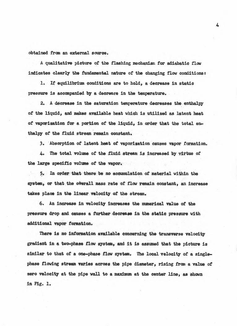
If an energy balance

(A) to (B) is taken, for

(1) U2 .1. (

ound the fl

teady state flow:1

P2V2 (II)

of Fig. 5 from point

Fig. 5. Piping system. C% base plane w: work to pump g: heat input z: height- above base

Equation (1) may also be expressed in differential

(2) d(PV) + d(KE) + d(m2,) + dU + dw dq

where the terms represent in order: flow work; external kinetic energy;

potential energy; internal energy; work done upon the surroundings; and

heat added from the surroundings. Changes in surface energy have been

1 Steady-state flow: applying the conseriation of mass principle to the system in order that no accumulation or depletion of material take place. Therefore, for steady-state flow, one pound of fluid entering at point (A) displaces one pound of fluid from the system at point (B).

12

neglected in equation (2) imee insufficient informati

available regarding the subject. When the elevation of points A and B

are the same above a reference plane, as is the case of a horizontal pipe,

the potential energy term may be dropped, simplifying the equation to:

(3) d(PV) + d(KE) dU dw gig dq

The kinetic energy is defined by KE = mv2 /eg. The value of 8 is

dependent upon the mechanism of fluid flow, and will be evaluated in a

later discussion.

The useful work, dw, done upon the surroundings is the maximum total

mechanical work obtainable frail the Frictional effects in the

system, however, reduce the net obtainable work recoverable because of the

dissipation of mechanical work into energy associated fluid friction.

In the form of an equation:

E4) dw m + dF

where dw represents the total possible mechanical work without friction;

d'w the available mechanical work when friction is present; and dF, the

work made unavailable as a result of the irreversible friction processes

which take place in the system. Combination of equations 0) and (4)

yields an energy balance for a flow process with friction

(5) d(PV) + d(KE) + dU + d'w dF dq

The units of the mechanical energy equation terms are those of

ft.-lb.(force)/lb.(mass) of flowing fluid. Used upon a mass of one pound

of fluid, the units of the equation become f t of fluid. These terms ex-

preseed in length unite are called "heads" (e.g,, the "friction head"),

and express the height Of a column of the fluid. Multiplying terms of the

13

equation by the fluid density converts the head into pressure units. An

example problem can perhaps best illustrate.

Example: The friction head observed for the flow of an

oil (sp. gr. = 0.8) through a piping system

is 2.0 feet. What is the decrease in static

pressure caused by frictional effects?

P = 2.0 ft. x 0.8 x §2.5 4.1D. x 1 sq.ft. = 0.7 psi.

cu.ft. 144 sq. in.

One-Phase Flow

The frictional loss of mechanical energy may be evaluated for a

single-phase system by means of the Fanning equation, in consistent

units:

(6) F = 4fliv2 = 4fLG2

2gcn 2geD1 2

where F is the friction head, in feet, of the flowing fluid as observed

over a finite duct length, L; D is the inside diameter of the duct; ,

the density of the flowing fluid; v, the linear velocity of the fluid

stream; ge, a conversion factor; G, the mass velocity;1 and f, the Fanning

friction factor which varies with the Reynolds number (Dv/oh4) = (DG//4).

The friction head, F, may be expressed in terms of the pressure drop

due to friction over the length of pipe, L:

(7) P = F x p 4fLG2 2gc]p/3

1 Mass velocityt the product of density and velocity, convenient to

use in place of linear velocity and density, especially in the case of

gases; since this quantity is independent of pressure and temperature,

whereas both linear velocity and density change with these variables

(Badger and McCabe, 1, p. 135).

Equations (6) and (7) apply only to steady flow conditions in (dr-

cular pipes running full of fluid of constant density.

When the density varies over the length of pipe, as in the flow of

s or the non- isothermal flow of liquids, the Fanning equatien must

be used in differential form:

(3) d( = d(F/3 ) = 41102

dx dx 2g0D/0

Equation (3) applies to a differential length of pipe, dx, over

which the density may be considered constant.

The dimensionless Fanning friction factor has been shown (Ferry, 16,

p.331) to be a function of the Reynolds number for pipes and ducts of all

cross -sectional shapes. Experiments conducted with artificially roughened

showed that f is a function of pipe wall roughness at sufficiently

large Reynolds numbers (Colebrook and White, 6 ).

Figure 6 shows the friction factor, f, as ordinates, plotted vs.

the Reynolds number, Dv/044G, as abscissas, for ordinary types of pipe.

Curve A of Fig. 6 holds for all pipes and is theoretically deducible

for considerations of vim** flow. The equation of the sum is:

(7) f = OA so 1.4

Dv/ Re

Curve C of Fig. 6 represents caneistet c ttra. obtained for smooth

copper lead and glass tubes. s ccordi. According

the equation of this curve is:

(10) f = 0.00140 0.125 k

0.32

Koo and McAdams (7) )

Curve D of Fig. 6 represents practically all known data for cle

commercial iron and steel pipe. The data lies within a band of t 10 percent

of the curve. According to Wilson, McAdams and Seltzer (13) the equation

of this curve is:

(11) f = 0.0035 + 0.264 (k)0.42

When Dvf/u., increases past the Reynolds criterion (Re = 2100),

rises rapidly as Dv,/,44 increases (e.g., curve 13, Ag. 6) and then falls

off along a curve of gradually decreasing slope (curve C or D, Fig. 6).

The location of curve B depends to a large extent upon the nature of the

wetted pipe surface (Ferry, 16, P. 383).

1.00

0 4-

0 0

.01 &_ -

LL

.001 -2 10 los lo4 lo 5 106

DG Reynolds number, Re::.1-)2--=

Fig. 6. Fanning friction factors, f, for straight ducts. (16)

A: viscous flow C: smooth tubes

B: critical region D: commercial pipe

15

16

Moody (15) has correlated the Fanning friction ac or vs. Reynolds

nuMber with relatrre relative pipe roughness as a parameter. The relative rough-

ness is obtained from an auxiliary plot of relative roughness vs. pipe

diameter, for various types of commercial pipe (;dr OMR tubing, steel, cast

iron, concrete, etc.).

investigation ras to determine

d in what manner, the conventi phase flow equations could

tared to make them applicable for predicting frictional pressure

drops due to the flew of fleshing liquids. The basis for the following

analysis was the plater, of ring flow developed in the Physical Analysis

section of this paper.

The combined frictional pressure drop at a cross-sec

piping system conveying a flashing fluid is assumed to be

pressure drops due to vapor and liquid flow, respectively;

( 12) [414rd I

The individual pre ours drop tributi

culated from the Fanning equations

(13)

( 14 )

where 0( and are coefficients peculiar to the two-phase system.

17

Martinelli, Putnum and Lockhart (13) utilize the same approach to a two-

phase, two-component flow problem in which both phases flow in the viscous

region.

The friction factors of equations (13) and (14) are based upon

modified Reynolds numbers:

(15) fv1 = ()v1 ( )V 1

(16) I'll = 4' (1q9-) r 0 Y (V)LI

Based upon inferences drawn in the section entitled "Physical Analysis",

the terms of equations (13) through (16) have the f01/04ing identity:

1. The velocity terms of equations (15) and (16) are both equal to

the average velocity of the fluid stream at cross-section (1). The average

velocity is determined by the average density at this cross-section.

2. The diameter terms of equations (13) through (16) are all equal

to the inside diameter of the pipe under consideration.

3. The density terms of equations (13) and (15) refer to the vapor

density at cross -section (1), and the density terms of equations (14) and

(16) refer to the liquid density at the same cross-section.

4. The viscosity terms in equations (15) and (16) refer to the

viscosity of the vapor and liquid, respectively, at cross-section (1).

5. The functions in equations (15) and (16) are identical to them,

functions describing the variation of friction factor vs. Reynolds number

for one-phase flow in the pipe under consideration (Fig. 6).

The coefficients oc, lb, a and b, in equations (13) through (16) were

unknown. Experimental data Compiled in this investigation were used to

evaluate these unknowns.

18

sepia of the Test Apparatus

Data used in this paper were obtained in an insulated horizontal

feet pipe. Calculations showed that the heat loss from the test pipe

and eared be neglected (see Sample Calculations). The

empertmente data are therefore for an adiabatic process.1

The enthalpy change for this flow process can be shown to equal

the change in kinetic energy, and for small values of kinetic energy

the process approaches an isanthalpic process, which greatly simplifies

the mathematical treatment.2

(17)

a) d(PV) + d(KE) + dr dq d'w (equation 5)

b) d'w PdV (the usefe mechanical expansion work)

c) dU = dq - PdV (definition of internal energy)

d) d(PV) + d(KE) + dF la 0 (colehining a, b and c)

e) dR = Tds VdE (definition)

f) d(PV) PdV + VdP Tds (substituting 410

g) PdV + Tds + d(KE) + dr m o (combining d and 0 h) dq Oda (for an irreversible process)

i) dq + dF = Tds (for an irreversible frictional process)

j) dq 2: 0 (for an adiabatic process)

k) dF = Tds

1 An adiabatic process is carried out in such a manner that no heat is absorbed or evolved by a system.

2 Isenthaipic processes take place without change in the enthalpy, or heat content of the system.

19

1) fdV + dll + d(KE) = 0 (combining g and e)

PdV = dtw * 0 (since no useful expansion work is done)

n) = . -d(KE) (combining m and n)

o) &II= - EKE (in an incremental form)

Therefore, the change in enthalpy of the flow process studied equals

the kinetic energy change of the fluid, since no machines for introducing

or withdrawing mechanical energy were present in the system, and the flow

was adiabatic. This kinetic energy change equals (mv2/0gc)2 (mv2/0f01

The coefficient, e, depends upon the type of flow, either viscous or

turbulent, and is equal to 1.0 for viscous flow and 2.0 for turbulent

flow (Perry, 16, p. 376). On a numerical basis, the heat equivalent of

the kinetic energy change was so small that it could be neglected, for

practical purposes (see Sample Calculations).

LITERATURE URVEY

A large portion of the pal/Sited material concerning two-phase,

fluid flow in pipes resulted from studies conducted at the University

of California Agricultural Experiment Station (3 12, 14). The primary

objective of the study was to arrive at a satisfactory method for

estimating the pipe size of fuel lines serving orchard heaters, and

various liquid-air mixtures, pipe sizes and fluid temperatures were used

in obtaining the experimental measurements, The California work was

concerned with two-component flow, and the proposed method of calculation

utilized a friction factor based on liquid properties alone, used in

tion with a "flow modulus* which was correlated in terms

properties and the cross-sectional area of flow occupied by the liquid.

Deviations of calculated friction heads from experimental measurements

re within thirty percent. The flow modulus correlations limited

application of the method to two...phase tsewrsomPonient flow 461010

the systems studied.

Martinelli at al. (13) attempted to extend the method and relation-

ships developed in the above studies to predict the pressure drops during

ow of flashing water-emssmixiOriss, but the limitations of the two-

two-component flow analysis remained, No data appeared which could

in this paper, and as before, no attempt was made to correlate

terms of the standard frictional pressure drop equations.

The first published data for the pressure drop due to the flow of a

flashing mixture wee presented by Bottomley (4). His observations cen-

tered about one run performed on a marine boiler within a narrow range of

conditions, and necessari27 limited the conelmetens to the observation

that :Lines carrying flashing fluids should be much larger than those

carrying the equivalent flow rates of a single liquid phase. The data

the marine boiler test run were presented in conjunction with a

thorough discussion of the flow of boiling water through a converging

mole* Information concerning the flow of a flashing water-steam mixture

through an orifice 1107 be useful for the design of experimental facilities

for further study of the flow of flashing water- steam mixtures through

pipes. For this reason, reference was made to the same article in the

Future Recommendations section of this paper.

Be 2

the flow ipes. Their ob-

servations and data °suited from erosion studies conducted for the bends

of boiler drain lines, since it was believed that increased erosion re-

ulted from acceleratiOn of the moving fluid due to additiessl vapor for-

mation during flows its desired result of the investigation was the

evolution of a goomesta method for designing the drain lines which wou

compensate for velocity increases and thereby reduce erosion.

The method proposed consisted of a graphical integration of the

cal energy equation (equation 1). The friction factor term used

authors was an average of all observed friction factors for the

and existing 1 conditions. Use of this average value was

since flow conditione encountered in the test system, the drain

limes of a Detroit, Michigan power plant were substantially constant

yielding friction factors which varied within a twenty percent band. Since

no attempt was made to correlate friction factors in terms of physical

properties or flow conditions, the method of calculation was limited to

drain line design over the same range of operating conditions and to the

water -steam system only. The method

of similar stationary equipment.

In addition to the foregoing, Be jamin and Miller noted the existence

of a critical ratio of inlet and outlet pressures for novena experimental

runs, similar to critical pressure and acoustic velocity relationships

known to exist for the expansion of single phase fluids flowing through

ive data

is of value to designers

pipes, orifices, and convergent hassles.1

A stepwise calculation of premium drop for the design of tubular

heaters handling flashing hydrocarbons has been proposed by Kraft (11).

The friction factor term used in the Yenning equation was based on liquid

properties only, while the velocity term was determined by combining

properties of the two phases on a weight basis. The method appeared to

approach actual conditions for the type of heaters investigated.

Conclusions drawn from the published work include:

1. The flow mechanism for flashing mixtures was unknown, and the

approach used was to attempt correlation of frictional pressure drops

in terms of gross flow properties.

2. Friction based on been used almost

exclusively, despite their failure to reproduce experimental observations

within the usual range of error of the Fanning equation-Reynolds number-

friction factor relationships for one phase fluid flow.

3. The need for further investigation of the flow of flashing fluids

exists, especially for the development of a satisfactory flow picture and

associated mathematical analysis. Using as a basis the widely accepted

Acoustic velocity: the velocity of sound in the fluid medium.

When the linear velocity of a fluid is equal to its acoustic

velocity, the maximum flow rate possible through the pipe or orifice for

the given upstream conditions is obtained, and no further increase in flow

can result from any change in downstream conditions. Consideration of acoustic velocity and critical pressure ratios is

unavoidable in the treatment of high velocity fluid flow problems, but has

been disregarded in this paper since the linear velocities here encountered

(vim. = 150 ft./see.) fall far short of the acoustic velocity of either

fluid stream ( > 1000 ft. /sec.). Relationships which permit calculation of

acoustic velocities based on fluid properties are available in the

literature (Brawn, 5, p. 200) (Ferry, 16, p. 375).

23

flow equations and correlations would enable prediction of pressure drops

for the flow of any flashing mixture in commercial pipes.

XPER1MI NTAL EQUIPTIENT

The advantages of using the steam-water system for this investigation

were: availability in the laboratory, ease of handling and abundance of

physical property data in the literature. The experimental apparatus

(Plate I), however, is not limited to this system.

The sequence of events which took place in the test apparatus were

as follows:

1. Steam was injected into cold water in a mixer, and the mixture

allowed to come to saturation equilibrium conditions.

2. Excess steam was separated from the saturated liquid in an

entrainment separator.

3. Saturated liquid and excess vapor were injected through a second

mixer into the test line.

4. The discharge of the test line was condensed and cooled in a

heat exchanger and collected.

5. Flow conditions were recorded from gauges and meters strategically

located throughout the system.

Steam was supplied to the system from a steam,heated, jacketed kettle.

The steam generated was fed to a vertical mixer in which it was injected

into a controlled stream of cold water from the laboratory mains. Plate II

is a detailed sketch of this first mixer. Pressure differentials dis-

tributed by lines (F) caused piston (C) to adjust its position, mixing

EXPLANATION OF PLATE I

Schematic diagram of experimental apparatus

C : tared container D : drain ES: entrainment separator F : Flowrator G : gauge HC: electric heating coil K : steam-generating kettle M : Merriam mercury well manometer MV: manometer valve MX: mixer SG: sight glass ST: surge tank T steam trap TP: test pipe V valve

PLATE I

UP W AT DF P

Dotaiis of first mixer

A: stainless steel end fitting B: one-half inch braes pipe C: piston D: one and one -het inch tree pipe

jacket Es adjuateent valves Fs one-eighth inch copper tubing L: cold water inlet V: steam inlet

E--

PLATE

26

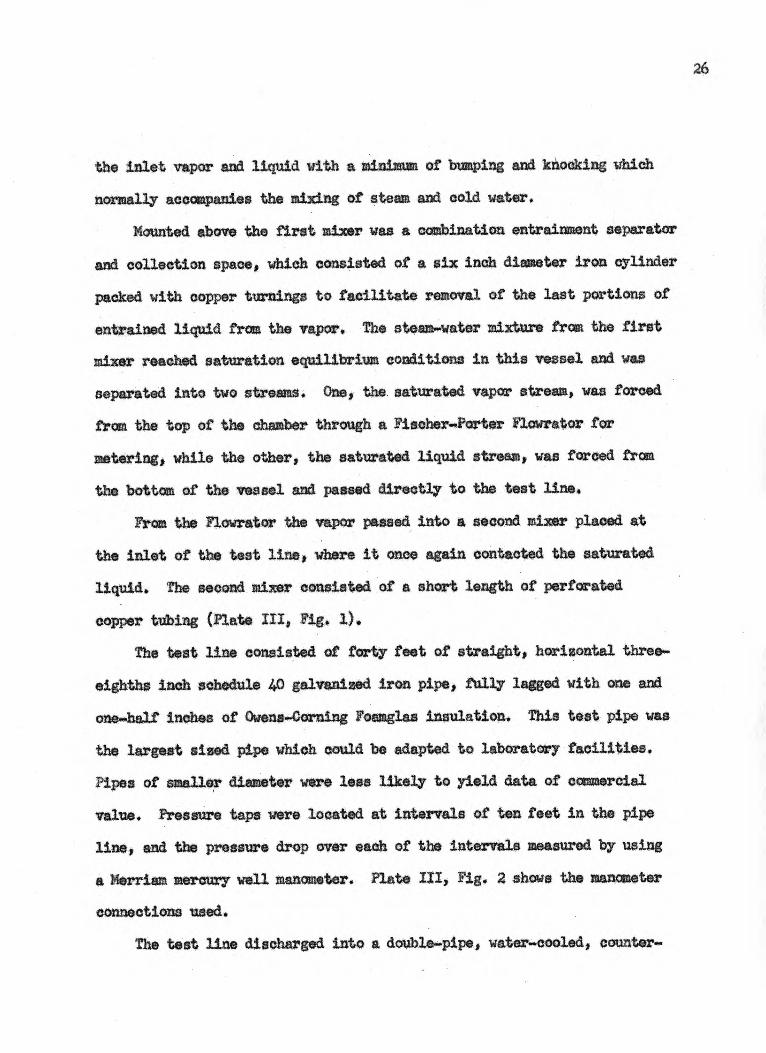
the inlet vapor and liquid with a minimum of bumping and knocking which

normally accompanies the mixing of steam and cold water.

Mounted above the first mixer was a combination entrainment separator

and collection space, which consisted of a six inch diameter iron cylinder

peaked with copper turnings to facilitate removal of the last portions of

entrained liquid from the vapor. The steam-water mixture from the first

mixer reached saturation equilibrium conditions in this vessel and see

separated into two streams. One, the saturated vapor stream, was forced

from the top of the chamber through a Fischer-Porter Flowrator for

metering, while the other, the saturated liquid stream, was forced from

the bottom of the vessel and passed directly to the test line.

the Flowrator the vapor passed into a second mixer placed at

the inlet of the test line, where it once again contacted the saturated

liquid. The second mixer consisted of a short length of perforated

copper tubing (Plate III, Fig, 1).

the test line consisted of fert feet of straight, horizontal three-

eighths inch schedule 40 galvanised iron pipe, fully lagged with one and

one-half inches of Owene4orming Foamglas insulation. This test pipe was

the largest sized pipe which could be adapted to laboratory facilities.

Pipes of sreller diameter were less likely to yield data of commercial

value. Pressure taps were located at intervals of ten feet in the pipe

line, end the pressure drop over each of the intervals measured by using

a Merriam mercury well manometer. Plate III, Fig. 2 shows the manometer

connections used.

The test line discharged into a double-pipe, water-cooled, counter-

EXPLANATION OF PLATE III

Fig. 1. Sectional view of second mixer

ig. 2.

V: vapor inlet L: liquid inlet

Manometer conn ot

A: test pipe B: bleeding petcocks C: Merriam mercury well

manometer D: valves for dampening

line pulsations

Z/Z

PLATE M

11/4N

Fig. I.

Fig. 2.

current heat exchanger, which in turn discharged into a collection vessel

or drain, as was desired.

Auxiliary equipment included a large surge tank placed in the

laboratory water line to dampen pulsations which are characteristic of

the College water system; a small surge tank in the first manometer line,

to dampen pulsations caused by the second mixer; a series of valves on the

manometer lines to dampen pulsations transmitted from the test pipe; an in-

let and outlet pressure gauge, to ascertain inlet fluid characteristics and

check on the overall pressure drop shown on the mercury manometers, resp410..

tively; valves and pressure gauges used in conjunction with the steam generating

facilities; and an electrical heater placed between the entrainment separator

and vapor Flowrator. Adjustment of the electrical input to the heater enabled

condensation in the Flowrator tube to be reduced to a minimum, thereby re-

ducing the "liquid drag"1 effect on the stainless steel float.

The operating range of the test line was limited by the maximum in-

ternal working pressure of the kettle (40 psia.), and the line water

pressure at the discharge of the first mixer (45 psia.).

Attempts to feed laboratory steam directly into the experimental

apparatus resulted in difficulty in maintaining constant conditions.

1 Liquid drag: the Fischer-Porter Flowrator operates on the principle

that a different orifice area exists for each rate of flow, and as a

consequence, the differential pressure is constant. The float remains in

a fixed (but rotating) position when the differential pressure just

balances the weight of the float. Liquid drag is caused by the accumulation

of condensate in the tapered Flowrator tube and manifests itself by 1) re- ducing the orifice area for a particular position of the plummet, thereby

altering the differential pressure, and 2) increasing the apparent weight

of the calibrated plummet.

29

EXPERIMENTAL PROCEDURE

Calibration of the test equipment preceded the actual trial runs.

Calibrated were: 1) the vapor Flowrator and 2) the test line, using

water only. The test line showed favorable results on the basis of a

Fanning equation correlation.

The operating procedure for an actual test run follows. the symbols

refer to notations in Plate I:

1. The manometer lines were bled by opening valves V8,11,12

MV1_5 and the pair of petcocks on each manometer for this purpose.

Bleeding continued for about fifteen minutes in order to assure complete

removal of air from the manometer system. Bleeding petcocks were closed

and flow was stopped by closing valve V12. Zero manometer readings were

then taken.

2. Valve V12 was opened and valve Vs adjusted to give a flow rate

sufficient to keep the manometer lines filled with water. Valves Vl and 3

were opened to begin steam generation. When gauge G1 indicated sufficient

steam pressure, valves V4 and V10 were opened, admitting steam to the

mixer and cooling water to the heat exchanger, respectively.

3. When the level of liquid in the entrainment separator sight glass

indicated saturation of the contents, valve V9 was opened, admitting

saturated water vapor to the vapor Flowrator, thence to the test line.

Electrical power supplied to the auxiliary heating coil was adjusted so

that condensation in the Flowrator was reduced to a minimum.

4. Valves V4, 8 and 9 were adjusted to vary inlet conditions.

30

5. Valves MV/..4 were adjusted to dampen pulsations in the manometer

line.

6. When the apparatus had adjusted to a dynamic equilibrium condition

as indicated by a constant level of liquid in the entrainment separator,

readings of F2; M1, 2, 3, 4 ; G4, 5 and

the total weight rate of flow were

obtained. The total weight rate of discharge was obtained by collecting

the cooled discharge from the test line in a tared container, over a

measured time interval.

7. Valves 740 so 9 were adjusted to give new inlet conditions, and

the procedure of steps 3 to 7 repeated.

Care had to be exercised when *warding data, in order to insure

that no change took place in the inlet conditions over the time interval

required for reading instruments and recording those readings.

THE DATA

The experimental data obtained in this investigation are tabulated

in Tables 1, 2 and 3. Table 2 is the steam Flowrator calibration;

Table 3, a comparison of observed pressure drops and pressure drops cal-

culated with the Fanning equation, for the flow of water only; and

Table 1, pressure drop data for the flow of flashing steam-water mixtures

for various inlet conditions.

Weight rates of discharge were obtained by collecting the cooled

effluent from the test line over a measured time interval in a tared

container.

Calibration of the steam Flowrator was made on a volumetric rate

31

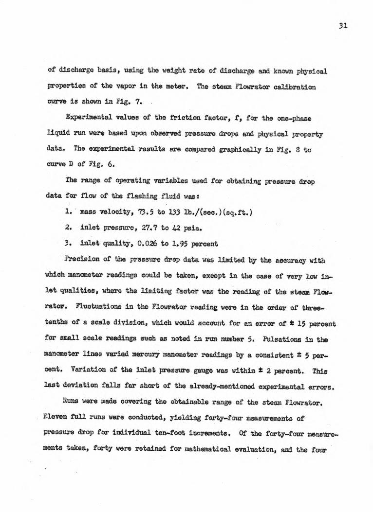
of discharge basis, using the weight rate of discharge and known physical

properties of the vapor in the meter. The steam Flowrator calibration

curve is shown in Fig. 7.

Experimental values of the friction factor, f, for the one-phase

liquid run were based upon observed pressure drops and physical property

data. The experimental results are compared graphically in Fig. 8 to

curve D of Fig. 6.

The range of operating variables used for obtaining pressure drop

data for flow of the flashing fluid was:

1. mass velocity, 73.5 to 133 lb./(sec.)(sq.ft.)

2. inlet pressure, 27.7 to 42 psia.

3. inlet quality, 0.026 to 1.95 percent

Frecision of the pressure drop data was limited by the accuracy with

which manometer readings could be taken, except in the case of very low in-

let qualities, where the limiting factor was the reading of the steam Flow-

rater. Fluctuations in the Flowrator reading were in the order of three-

tenths of a scale division, which would account for an error of * 15 percent

for small scale readings such as noted in run number 5. Pulsations in the

manometer lines varied mercury manometer readings by a consistent t 5 per-

cent. Variation of the inlet pressure gauge was within t 2 percent. This

last deviation folls far short of the already-mentioned experimental errors,

Runs were made covering the obtainable range of the steam Flowrator.

Eleven full runs were conducted, yielding forty-four measurements of

pressure drop for individual ten-foot increments. Of the forty-four measure-

ments taken, forty were retained for mathematical evaluation, and the four

32

obtained from run number seven omitted, due to a fluctuation in inlet

conditions during the course of recording data for that run.

ANALYSI6- OF THE DATA

Evaluation of Terms

The measurements taken for the flow of a flashing mixture through the

test line were directed toward obtaining data which could be utilized in

some form of the Fanning equation and friction factor vs. Reynolds number

correlations.

Experimentally observed pressure drops consisted of two parts:

1) that which was due to friction (friction head), and 2) that which was

due to an increase in the kinetic energy the flowing stream (velocity

head). Since the properties of the fluid streams were fixed by the inlet

conditions and the combined pressure drop, these properties were used to

describe the dynamic conditions of the two-phase flow. However, when the

merit of the proposed method for calculating friction head was to be

evaluated, results calculated could only be compared to the experimental

friction heads.

Inlet qualities were determined using the steam Flowrator calibration

and weight rate of discharge, 14, combined with the experimentally deter-

mined static pressure:

(18) a) wy m /01, x (VA)

b) Q = WV = wV

wV wL w

where WV = weight rate of discharge of vapor; /3 V, the vapor density at the

inlet pressure; arad (V/t) the volumetric rate of discharge

the steam Fiowrator calibration. The mass velocity for sac run w

culated by dividing the total weight rate of discharge by the inside cross -

sectional area of the teat pipe since .G w/A.

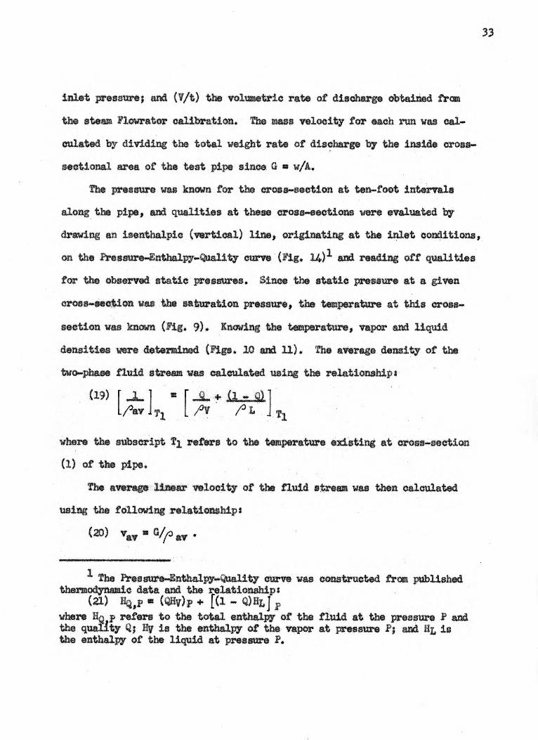
The pressure was known for the cross- section at ten-toot ntervals

along the pipe, and qualities at these cross-sections were ev

drawing an isenthalpic (vertical) line, originating at the in

on the Pressure..Enthalpy-Quality curve (Fig. 14) and reading

for the observed static pressures. Since the static pressure

cross- section was the saturation pressure, the temperature at

uated by

et conditions,

off qualities

at a given

this cross

section was known (Fig, 9). Knowing the temperature, vapor and liquid

densities were determined (Figs. 10 and 11). The average density of the

two-phase fluid stream was calculated using the relationship:

where

(19) .1. q)

li'av

1

v /' I

subscript T1 s to the temperature existing at cross

(1) of the pipe.

The average velocity of the fluid stream was then

the following relationship:

(20) vi 0 G/;(.) a .

The Pressure-Enthalpy-Quality curve was constructed thermodynamic data and the relationship:

(21) HQ,p (41v)p [(1 - 041 p where HQ p refers to the total enthalpy of the fluid at the qua) ty Q; Hy is the enthalpy of the vapor at pressure the enthalpy of the liquid at pressure P.

culated

lisped

assure P and and H is

33

34

Methods Used to Determine Pressure Drops for the Flow of Flashing Fluids

A large portion of the early work in this investigation was con-

ducted on a "cut-and-try" basis, since little or no information was

available in the literature to serve as a guidepost to procedure.

Tried first were a series of successive approximations based upon

a friction factor defined by liquid properties, and liquid velocity ad-

justed for vapor formation. Results obtained were uneatisfactory.

Next tried was a method in which gas and liquid properties were com-

bined on a weight basis to yield "pseudo" properties which were then used

to determine the value of the Reynolds number and the friction factor for

the Fanning equation. This method was unsatisfactory since combination

of vapor and liquid viscosity on a weight basis yielded a pseudo viscosity

of numerical value much the same as that of the liquid, in the range of

qualities observed. The friction factor, therefore, corresponded to a

liquid friction factor, as in the first method tried.

The third method tried utilized only gas properties in the Fanning

equation and for the calculation of Reynolds number. A friction factor

was calculated by substituting experimental pressure drops and known gas

properties of the fluid stream. This friction factor was then compared

to the friction factor of curve D, Fig. 6. The calculated values showed

a marked resemblance to curve D when plotted on the same co-ordinates,

but showed wide scattering and a general tendency to fall below the I) curve.

All attempts to rationalize the deviation from curve D as a function of

physical properties or flow conditions failed. The inference drawn from

35

this method was that gas properties are most important in determining

the pressure drop for tha flow of a fieehing liquid.

On the basis of the foregoing obeerretion, another method utilizing

only gas properties was tried. The relationships employed are expressed

in equation forms

(22) Dv ec (02 x S)*

(23) Re se ya Al

(24) ALAI/ 4fG2.a dx 2g/3 09V

whers Dy ears to a diameter based. upon the cross -se occupied

by the vapor' and S, the fractional part of ths arose-seSties occupied by

the vapor.

An overall average error of less than plus one percent was obtained,

kith an average deviation of ten percent for the data consisting of pressure

drops for the ten runs over the pipe line composed of four ten-foot sections

or a total of forty ten foot sections.

Despite the excellent results, however, there were evident shor

comings of the method: 1) where the quality is zero, the pressure drop

was indeterminate; this was unsatisfactory since the saturated liquid of

zero percent quality does experience a pressure drop, and 2) there was

no justification for the use of a diameter term based on cross-sectional

area occupied by the gas to calculate the Reynolds number, nor for the use

of the total inside diameter in the Fanning equation.

The weaknesses of the above method were absent when the mathematical

analysis represented by equations (12) through (16) and the ring flow

36

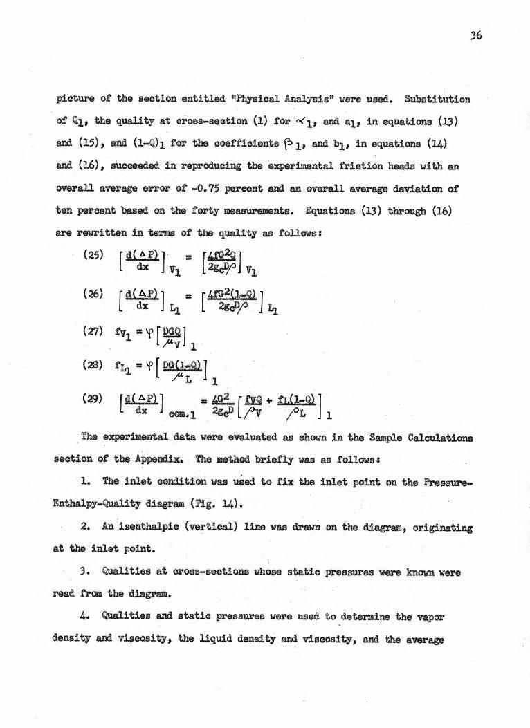
picture of the section entitled "Physical Analysis" were used. Substitution

of Q1, the quality at cross-section (1) for 0(1, and al, in equations (13)

and (15), and (1-Q)1 for the coefficient 510 and b1, in equations (14)

and (16), succeeded in reproducing the experimental friction heads with an

overall average error of -0.75 percent and an overall average deviation of

ten percent based on the forty measurements. Equations (13) through (16)

are rewritten in terms of the quality as follows:

(25) raoio r411G2 Q1 dx ,vl v].

(26) r dc AP) 1 = r aG2(1-c0 dx J LI [ 2gclr .1 LI

(27) fvl = ̀ )rD.G q 1 L. /ay J

(28) fLi = { DO (1_Q)

/41. 1

(29) rd(Ap)1 = itgl_rag fr.(1 -U) L dx JJ com.1 2gcP 1.rn 1

The experimental data were evaluated as shown in the Sample Calculations

Section of the Appendix. The method briefly was as follows:

1. The inlet condition was used to fix the inlet point on the Pressure-

Enthalpy-Quality diagram (Fig. 14).

2. An i enthalpic (vertical) line was drawn on the diagram, originating

at the inlet point.

3. Qualities at cross-sections whose static pressures were known were

read from the diagram.

4. Qualities and static pressures were used to determine the vapor

density and viscosity, the liquid density and viscosity, and the average

37

velocity at the given cross-sections.

5. Reynolds numbers for the vapor and liquid phases were calculated

and from these the respective Fanning friction factors Obtained.

6. The combined rate of change of static pressure, d( nP)/dx, was

calculated at the giv en cross-sections by using equation 29.

7. The caleulated frictional pressure drops, AP(calo.) were ob-

tained for each ten -fit section by graphically integrating [d(bP)/dx]can.

versus L.

8. The pressure drape resulting from the kinetic energy increase of

the flowing fluid were calculated and subtracted from the experimentally

observed combined pressure drops, leaving experimental friction heads only.

9. Calculated friction heads were compared to the experimental

friction heads on a percentage basis to determine the relative agreement

between the two.

Experimental data and calculations of the frictional pressure drops

for the flow of the flashing water-steam mixtures are presented in Table 1.

itNA

nt-r&f§

trtceN0

0 X

401401 .44010

rs -4 $A

4

-4 CI

tiN

tO

U

"'lc 4;4'1%

oeo czt PoR

g144 tO

0 CI

Cr%

IN..8A

4gd M

OO

to ,s.%

44"

44 C

V eel 3 U

N +

JO tO

(1%

,

8 4§§kkkk

lb lb

lb .14

44,a4k V

gif4

lblblblblblblblblb C

J C

4I-I C

'S

k§44,1/§1 ipii,p34$is

1

&§U

A

f',9;g*eRce,gv7Feihi

II IS

*

000000000 g

it=

tall tO'

8 8 8 td

0 *50

5 .4.4.. 0000000000

-.o ifo

008.6414044

WI I

dacUddadd

it\ ":

ri 0 0

d d di C

S

sti 0. 0 :I

419.0 $0"0 *OT Te'15 Trt OV't oos6 051 00 *Z nal IT /47T n*0 12'0 60'0 05"OT £I'5 ase fir '/, 88' k5"Z OI 41'1 57'0 6r0 90'1.0 1894, 00'7 98T LVT R5'9 L5*E Trt Uri 6 55*0 /Z*0 Z1-*0 50"0 C0'7 06°Z 8-C°Z 46'1 60"/ LL7 ZI"Z Cie,'T 8 WI 'WO 44'"0 00"0 Et "L 50'7 06'Z ZZIPZ 80"9 Ore 04,7 40.Z 9 66"0 OlrO Lr0 140'0 0£"7 57'Z WI 60'I 06'5 06"g n'I C6"0 5 /VT M*0 U*4 00'0 EZ'L 00"7 98*Z 8C2 W9 WE OWT 50*Z / 9CE 05'0 WO 60%) 89"7 130'E 67 *Z 5Z"4 OZ"/ 00°E ECZ E C6'0 1.£"0 er0 1,0'0 0£'5 ev-e Orme tl.°1 £T'5 80"C OT'Z 7C'T 90*T 01".0 6I*0 L0'0 58'5 07' 9C"C 1,6.1 00'9 59*E 597 00*Z

Q a

-Tod 4 (

sans

s

4doap t

No I

tsW-toj asma2er4uT reandsa2 Lci :

'Tod 4(-0/so)("*°) Jay : T ape

Uri T,450 z5C.0 Otr0 19141) 09900so 09ctro 041900.0 07900s0 04i900.0 6vro 60C.0) 917r0 Oro 09900.0 0900.0 01900.0 SE9o0.o 5C900.0 t' 'T

trot C5ro 410.4 Ece.0 M.° 00L00.0 E8900.0 9L900.0 54900°0 .74900.0 C15.0 vtC.0 T.R.0 taro 65r01 o5h0o0 Moro 0E400.0 oChoo-o 5z400.o 189.0 riro TT-CV tero ZOI*0 z69oo.0 vi.900.0 zid9o3.0 o4900.0 99900.0 094.0 CO e aerie 460.0 CO 49900.0 9590040 05900.0 05900.0 05900.o 256.0 ter° a£.0 iaa.0 94T.0 zi.900.0 09900.0 55900.0 %% WO 05900.0 970.-C 605.0 M.° tiro coe-cw 8oLoo°0 06900'0 a900.0 84900.o 54900.0 IZL*0 6Z,VD C5V0 6ir0 Qtro 50,00"0 0/49000 49900.0 299000 z9900.0 03'0 477'7'0 60C*0 Ut.0 9/3"0 49900.0 54903.0 oL900.0 99900%) 799014.0

rc OT 6

9 5 4, C

no.

1 2 3 4 5 6 21 8 1.92 9 1.71

in 2.31 U 2.32

2.2 539 4484

9 6.91 6.46 3.71

.83 6.41 3.74

Average percent section

Avery ecviati

27

- 9. 83 + 5.85 2 21.20 74 18.17

Percentage error :Average s

poxP.-oa1cti 100 :percent :error

B --P, R nzttr voik

Average percent deviation per ru4

+16.23 4. 0.96 +1.35

+15.60 + 6.00 +4.92

32" + 0.61 000.24

12.01 10.52 3.38 * 2.19 + 4.33 +5.57 + 2.43 3.62

7.04 40.10 +32.50 +15.21 19.11 3.22 oak 5.15 2.9$ 2.98

+ 0.47 0.36 + 8.2$ 0. 0.38 4075 41.72 - 4.53 - 3.66 3.52 6.42 +17.90 .19.135 .48.27 49.31 1 .42.42 9.11, +2.97 41.88 13.37

42

APPLICATION OF THE METHOD TO FLOW PROBLEMS

The most common fluid flow problem consists of predicting the

pressure drop suffered by the flow of a known weight of fluid through

a duct of known length for a finite period of time. Many variations of

the problem are possible but the discussion in this section will be

confined to the solution of this type.

Lhen analyzing the experimental measurements collected in this in-

vestigation, attempts were made to reproduce experimental pressure drops

by using physical property data for each of the phases, based on the ex-

perimental pressure drops. Since the results obtained showed good

agreement, the same type of analysis may be applied to flow problems in

which the pressure drop is the desired unknown. The method is as follows:

1. The inlet point is located on the Pressure -Enthalpy- Quality

diagram corresponding to fluid properties at the inlet of the pipe.

2. The path of the flashing flow process is established (e.g., for

an isenthalpic process a vertical line is drawn).

3. Pressure drops are selected, and the quality and physical pro-

perties evaluated at the static pressures which these pressure drops

determine. For example, if the inlet pressure is 40 psia., and pressure

drops of 5 psi. are selected, physical properties and qualities are

determined at 40, 35, 30, 25, etc., psis.

4. [d( o F) idX com. is calculated at each static pressure cor-

responding to a selected pressure drop by using equation (29).

5. Graphical integration of [dx/d( F) com. vs. 61), the selected

43

pressure drop* yields the length of pipe required to produce each

frictional pressure drop.

6. A smooth curve is drawn between the selected pressure drops

on * plot of Pf vs. L, and the value of the friction head corresponding

to the length of pipe being evaluated is picked off. In order to

determine the overall pressure drop for this pipe length, a velocity heed

term must be added to the friction head.

CONCLUSIONS

Ute of the ring flow plater* and the associated mathematical analysis

yielded satisfactory results ter the prediction of frictional pressure

drops duo to the adiabatic flow of a flashing water-steam mixture in

a horizontal three-eighths inch L1.8. schedule 40 galvanized iron pipe,

within the range of experimental data. The range of data observed wares

mass velocity, G* boo 73.5 to 133 ib./(sec.)(sq.ft.); inlet pressure*

27.7 to 42 psia.; and inlet quity, Q, 0.026 to 1.95 percent..

More detailed conclusions resulting from acceptance of the

presented analysis are as follows*

I. A flashing fluid exhibits an annular, ring type flow.

2. Linear velocities of the vapor and liquid streams increase

together and are the same at any cross-section downstream in the pipe.

3. The diameter of flow for booth phases approaches closely the in-

side diameter of tha pipe, even at low values of quality.

4. The overall head lose measured during flow of a flashing fluid

consists of velocity and friction head terms. There is little difficulty

associated ting vhelocity be eh are based on kinetic

energy changes only, for both one and two-phase flow problems. Combined

friction heads are the um of vapor and liquid flow contributions.

5. The coefficients, oe p b introduced to alter the Fanning

equation and Reynolds number relati to account for the unusual

flow conditions studied, serve merely to correct mass velocity terms to

actual individual phase, mass velocities (A g., MSS velocity of the

flowing vapor Q x 0).

6. Except for conditions of very low inlet quality, the gas phase

frictional contribution is most important in determining the overall

friction head.

The preceding conclusions were drawn from observations of the flow

of water-steam mixtures in an experimental apparatus and results ob-

tained after mathematical treatment. However, since the relationships

and physical picture presented are not inherently lis$ted to the water-

steam system or the experimental apparatus used, the method should be

applicable to the prediction of friction heads for the flow of other

liquid-vapor mixtures in any sized duct. Application to any system is

limited only by the availability of physical property data. Pipe size

type limitations are those associated with the Fanning equation and

Lou factor correlation; namely, long, straight, circular pipes

running full of fluid.

Although the purpose of this instigation concerned flow of a

flashing fluid, or a two-phase, one-component system, the picture and

mathematical analysis evolved may well serve as an approach to the question

of two -phase, two-component,flow problems as well.

45

AT OI FOR

In view of the satisfactory results obtained by applying the ring

flow picture and associated mathematical analysis to the flow of flashing

water-steam mixtures, further investigation of thelaathod is justified.

The possible paths of future studies includes

1, Critical investigation of the flow mechanism,.

24 Measurement of the pressure drops for the flow of other two-

phase, ent systems in different sized pipes and over extended

operating conditions.

The second path is the more preferable, since usefnl data capable

of application will be made immediately available. If the results of

these studies compare favorably with those obtained by the author and

presented in this paper, the method would be available for more general

pplication, and the inference may be drawn that the analysis presented

satisfactorily describes the flow picture.

The possible

is two-fold:

1. By using other systems and different pipe sizes in the existing

xperimental facilities.

By using other systems and different pipe sizes in a completely

revised experimental set-up.

Use of the existing facilities for further investigations necessarily

limits the extent of study to much the same operating ranges of mass

Conduct of Future study

n which con nu asurrnts could proceed

46

velocity, inlet pressure and inlet quality used in preparing this paper.

At the same time, this procedure would fail to establish whether or not

the method of calculation used is peculiar to the experimental apparatus

in which the measurements were taken.

Major revision of the existing facilities would enable extension of

the range of operating conditions beyond those attainable at present;

would ascertain the dependence of calculated results upon the apparatus

used; and would provide an excellent opportunity for correction of some

of the more troublesome features characteristic of the present facilities.

Several worthwhile innovations would be:

1. Improvement of the method whereby inlet qualities are estimated,

since considerable error is possible at present when measuring low values

of quality.

2. Removal of the uncertainty regarding the existence of saturation

equilibrium conditions in the liquid and vapor inlets, the result of

mixing saturated vapor and cold liquid.

3. A method whereby a more thorough dispersal of vapor bubbles in

the saturated liquid is obtained at the pipe inlet.

4. Introduction of the mixed liquid and vapor phases without

transmission of pulsations to the manometer system.

The author Awls that the advantages offered by a complete revision

of present facilities seriously outweigh the convenience of using the

existing apparatus without change.

47

Additional systems

Investigation of other two-phase, one-component systems is am

phasized in this section, since a primary consideration regarding the

usefulness of the analysis presented for predicting pressure drops

accompanying the flow of flashing fluids is whether or not the method

is confined only to the system studied (water-steam).

Choice of other systems depend upon the availability of thermo-

dynamic and physical property data, such as saturation properties,

enthalpies, densities and viscosities of the saturated vapor and liquid,

each as a function either of saturation pressures or temperatures;

commercial availability with regard to plentiful supply, uniform purity

and low unit price; and the relative ease of handling.

Toxicity, flammability, normal boiling point, chemical inertness

to air and moisture, and possible corrosion of materials employed in

the test equipment and storage facilitiss, all comprise the ease with

which a proposed substance is handled. The final criterion applied to

the choice of new systems is their frequency of occurrence in industrial

flow problems.

The author believes that investigation of the flow of flashing

trichloroethylene, a purified hydrocarbon such as hexane, and acetone,

would provide adequate proof regarding the generality of the method

presented, and at the same time supply data useful in rectifying many

industrial flow situations.

ons of the Experimental Apparatus

hen working with eye ether than ter-a econcay

operation dictates "closing" the piping system to allow cc4

recirculation of the fluid used. Work required for circulation may

be provided by a suitable pump strategically located in the apparatus.

In addition, the installation of store facilities such as a tank

would even flow through the system and act as a convenient reservoir,

permitting changes inflow rates without adding er removing material

from the closed system.

A series. of nozzles or

turat d vapor and liquid

ould appear to be more effec

plates designed to produce mi

suitable for injection to the test

than the kettle-first mixer-en-

trainment separator-vapor Flowrator-second mixer combination used for

the same purpose in this investigation. Varying the pressure and flow

rates of a near saturated or saturated liquid fed to the upstream side

of the nozzles or orifices would yield a wide range of possible saturated

vapor-liquid mixtures of different qualities at the downstream side of

the constrictions. An example is indicative of the process:

Examples Saturated trichloroethy is throttled isenthalpically through a nozzle. Estimate the exit quality if the downstream pressure is 100 pstg.; 50 Pais.

psis. 140

of the saturated Btu./lb. 42.00 of the saturated

vapor, Btu. /lb. 135.

(Perry, 16, p. 281)

eut]

100 50

11.10

122.15

49

wv) ((1

the process is

(0-0p2 + [(1

100 psis.*

e 4 (135 41 or

lbr

a.s .15)

* 27.8%

,equation 21)

nozzles or d i ions

may be accurately predicted, and upstream upstream.ron ,itions adjuste<3 yield

desired exit qualities and pressures.

One of the most desirable attributes of the rec

degree of ml-ging of

pulsation, as the re

treara which accompanies flow through orifices or nozzles.

Further suggested improvements include:

I.

in the nest

pressures

pressure-beesting device and heater

Mice* , therebY teasing the ranges of discharge

enatrietions. A jet pump used in conjunction with the

d system is

nod without

circulating pump should supply an adequate pressure range.

2. Decreasing the length of test pipe over which each individual

drop measurement is made, thereby increasing the accuracy of the

graphical integration and rendering the integration more sensitive to minor

fluctuations (04, the variation taking place in the erition menu

Re> 2100, <4000). Use of pressure tape placed at five.foot intervals

mad yield more tistactory pressure drop measurements.

50

ACKNOWLEDGEMENT

The author gratefully acknowledges the assistance

of Dr. Rollin t0, Taecker, whose constant interest and

efforts have aided materially in the development and

preparation of this paper; the cooperation of Dr.

Henry T. Ward for permitting the use of departmental

equipment for the investigation; and the labors and

understanding of Charlotte Gollobin, who so capably

accomplished the difficult task of transcription.

BIBLIOGRAPHY

W. L, McCabe.

emical engineering. k s

Benjamin, M. W. and J. G. Miller. Flow of a flashing mixture of water and atom Amer. Soc. Mech, Engre. Trans. 64, 657 (1942).

lter, L. M. K. and R. H. Kepner. Pressure drop accompanying two-component flow Indus. and Engg, Chem. 31, 426 (1939).

Bottomley, W. T. Flow of boiling water through orifices and pipes. North East Coast Inst. of Engra. and Shipbuilders). 53, 65 (1936).

Pi

pipes.

1936.

Brown, G. G.

Unit operations. New York: John Wiley and Sons. 1950.

Colebrook, C. F. and C. M. White. Experiments with fluid friction in roughened pips Roy. Soc. (London) A161, 367 (1937).

Drew, T. D., E. C. Kea and W. H. McAdams. The friction factor for clean round pipes. Amer. Inst. Chem. Engrs. Trans. 28, 56 (1933).

Fluid Dynamics (annual review). Indus. and Engg. Chem. 38, 7 (19

International Critical Tables, Volume given. Now York: McGraw-Hill. 1926.

eenan, J. H. and F. G. Keyes.

Thermodynamic properties of steam. Sons. 1946.

aft, W. W. Vacuum distillation o Chem. 27, #7 (1948)

tinelli, B. C. and D. B. Nelson.

Prediction of pressure drop during forced circulation of boiling water. Amer. Soo. Mech. Ewe. Trans. 70, 695 (1948).

r d

ks John Wiley and

52

(13) Martinelli, R. C., J. A. lutnam and R. W. Lookhert. Two-phase, two.component flow in the viscous region. Amer. Inst. Chem. Engrs. Trans. 42, 631 (1946).

(14) Martinelli, R. C., L. M. K. Benitez*, T. H. M. Taylor, E. G. Thomsen and E. U. Morrin.

Isothermal preemnre drop for two-phase, two-component flow in a horizontal pipe. Amer. Soc. Mech. Engrs. Trans. 66, 139 (1944).

(15) Moody, L. F.

Friction factors for pipe flow. Amer. Soc. Aech. Engrs. Trans. 66, 671 (1944).

(16) Perry, J. H.

Chemical engineers' handbook. Third Edition. New York: McGraw-Hill. 1950.

(17) Welker, W. H., W. K. Lewis, W. H. McAdams and E. R. Gilliland. Principles of chemical engineering. New 'York: McGraw-Hill. 1937.

(18) Wilson, R. E., W. H. McAdams and M. Seltzer. Flow of fluids through commercial pipe lines. Indus. and Engg. Chem. 14, 105 (1922).

54

Nomenclature

cross-sectional area, sq.ft.

a a constant, no units

b a constant, no units

D inside diameter, ft.

F force due to friction, (ft. lb. force) /(lb. mass)

of flowing fluid

Fanning friction factor, no units

G mass velocity, lb./(sec.)(sq.ft.)

local acceleration due to gravity, ft./sec.2

gc = 32.174 (lb. mass)(ft.) /(lb. force)(sec.2), dimensional constant

fI enthalpy, Btu. /lb.

L length ft.

mass, slugs

P pressure, lb./sq.in.

quality, no units

q heat input, Btu.

Re Reynolds number, no units

fraction of cross-sectional area occupied by the vapor, no units

entropy, Btu. /lb. -°F.

temperature, OF,

t time, min. or sec.

U internal energy, Btu. /lb.

volume, au. ft. velocity, ft./Sec.

weight rate of discharge, lb./1300.

distance along the pipe length, ft.

elevation above datum plane, ft.

no unite

P a constant, no units

A denotes an incremental value

denotes some function

it viscosity, lb./(ft.)(080.

/a density, lb. /cu.ft.

0 a constant, no units

404 refers o

2 refers cxro ecti0

ay. average

clam. combined vapor liquid contribution

F frictional

KB refers to kinetic energy term

L refers to the liquid phase

ov. overall, consisting of friction and ki

P refers to a given pressure

Q refers to a given quality

T refers to a given temperature

refers to the vapor phase

I in the apparatus

2 in the apparatus

55

energy contributions

56

Abbreviatio

Btu.

calf.

cu. ft,

British thermal units

calculated

cubic feet

cumulative

feet

kilogrsms

pounds

maximum

minutes

ohs. observed

psi. pounds per square inch

psis. pounds per square inch, absolute

sec. seconds

sq.ft. square feet

vel. velocity

wt. weight

57

Table 2. Vapor Flowator calibration.

0 1.8 1 21.6 2.93 6,45 0.323 41.7 10.5 3.39 2 21,3 1.53 3.37 0.337 40.2 10,7 1,60

3 16,6 2.05 4.52 0.215 43.7 10.2 2.19

4 12.1 1.38 3.03 0.138 43.2 10.3 1.42

5 19.1 2.35 5.18 0.259 39.2 10.8 2.80 6 5.3 0.40 0.88 0,029 39.5 10.8 0.31

7 9.0 0.80 1.76 0.088 40.7 10.4 0.84 8 13.9 1.20 2.64 0.176 42.0 10.2 1.73

58

Table 3. Calibration of the test pipe using water only.

: Time, : Wt. ,

Run t

no. i40.n. 2 lb.

: wL,

: lb,

Vels,

:

: stu

: AP obs.

2 f etu.e.

2 see.

1 5.0 21.3 0.0708 0.86 3,340 0.12 0.0120 2 5.0 35.0 0.1168 1.41 5,470 0.27 0.0102 3 5.0 59.3 2.39 9,300 0.65 0.0086 4 5.0 84.5 0.282 3.42 13,300 1.25 0,0080 5 4.0 88.3 0.368 4.46 17,350 1.99 0.0075 6 3.5 93.5 0.446 5.42 21,100 2.78 0.0071 7 3.0 95.5 0.532 6.45 25,100 4.16 0.0075 8 2.53 94.5 0.623 7.54 29,300 5.42 0.0071 9 2.0 82.6 0.688 8.35 32,500 6.81 0.0073

10 5.0 84.0 0.280 3.38 13,200 1.16 0.0076

Sample Calculations

Run number tour will be used to demonstrate the manner in Uhinh the

experimental data was used to determine the validity of equations (15)

through (29).

The Data

Steam Flowrator: 9.3

Inlet pressure gauge: 22.0 pd.

Manometer readings: Mis 4.80 in* rig

142s 6035 Jai Hi

m3: 8.,8 in. Ng

M4: 15.9 1414 Mg

Weight of discharges AS lb. Time interval: 7.0 rin.

Room temperatures 70 °F.

Calculations at the Inlet.,(4f4)

1. Weight Rate of Diadharge* w 68,5 lb. x 4n. .164 Ib./isc.

7.0 min. x 60 sec.

2. Quality. volumetric discharge of vapor Flouratert (V/t) 0 ou.ft./min.

(Fig. 7) inlet temperature at (22.0 + 14.7) * 36.7 psis., * 262° F. (Fig. 9) specific volume of the vapor at 262° F. a 11.50 =ft./1h. (Fig. 10) weight rate of discharge through vapor Flowrator wv = 0.88 cu.ft. x 1 m4.n. 1 lb. = .00128 1124 (equation 18a)

min. 60 sec. 11.50 ou.ft, sec. quality, Q = wviw = (.001281.164) x 100 = 0.7% (equation 18b)

3. Average Density. specific volume of the liquid at 262° F. = .0171 cuat./lb. (Fig. 11)

rage specific volume

(.79 x 10-2 x 11.50 esu. ft./lb.) + (.

0.109 cu.ft./lb. (equation 20)

ereags density, /o ay. = l lb./0.109 cu. t.

4. Maas Velocity. cross-sectional area of nominal 3/8" ached A .00133 sq.ft. (Perry, 16, p, 415)

mass velocity, 0 00.64 lb' .00133(sq.ft.)(0044)

Average Velocity. average velocity, v. , 4. (ette.)(sq.ft.)

.0171 cu.ft./lb.)

9.20 lbdou.ft.

6. Reynolds Number for the Vapor. viscosity of the vapor at 262° F.,

/Iv = .01372 centipoises (Fig. 12) so .01372/1488 = 1921 x lb,

(ft. (sec.) diameter of the pipe, D = .0411 ft. (Perry, 16 Reynolds number, Re * 1 b 2 4400

(equati

sec.

equation 21

see. x x lb.

7. Frict.one1 Pressure Drop Due to Vapor Flow. Fanning friction factor, f, at Re = 4400, = .0107 (curve D, Fig. 6) conversion factor, go = 32.17 ft./sece2 Fanning equation * ft( c.P)-1 = 441114 (equation 25)

L dx v 2g0DP V it"a c tonal pressure drop duo to vapor flow, rd(.64)-1

L dx 2 lb 2

x 32.17 x ft. x sec. x .157 lb./sq.in.),/ft.

8. Reynolds Number for the Liquid. viscosity of the liquid at 262° . /AL = .217 centipo se

= .217/1488 (Fig. 13)

x 1Q 4 lb. ft.) (sec.)

.9921 x ft. A sec.,

.46 x 10-4 lb.

(equation 28)

Reynolds umber, .0411 ft. x l.yt, lb. sec. x sq.ft. x

35,000

9. Fria Pressure Drop Due to Liquid Flow. Fanning friction factor, f, at Re = 35,000, .0065 (curve I), Fig. 6) Fanning equation In r a = 1402(1-Q) (equation 26)

I dx IL 2g0D/°14

61

Frictional pressure drop due to liquid flow, rd(LiP)1 dx 1

4* 4 x .000 x (124)2 x .?921 x .0171 a .019 (1b./eq. 2 x 32.17 x .0411 x 144

10. Cveral.l Frictional Pressure Drop.

.157 + .019 a 0.176 ( b. q. )/ft. (equation 12) dx

At.

Tn Fl

1. Quality. en isenthalpic (vertical) line is drawn on the Pressure-EnthalPY Quality curve (Fig. 14) originating at the inlet conditions of P a 36.7 psia. and Q 0.79 percent. This line is the locus of point conditions existing in the pipe line.

manometer reading at L = 10 ft. = 4.80 in. Hg density of mercury at room temperature, 70° F. as 13.54 glee.

(Perry, 16, p. 176) density of water at room temperature, 700 F. 0.998 g./oo.

(Perry, 16, p. 175) pressure drop, inches of water di 4.80 x (13 5

v 60.2 in. water pressure drop, engineering units

60.2 in x 1 ft. x 62.4 lb. x ap.;t4 2.18 lb./sq.in. 12 in. cu. ft. 144 cu.in,

static pressure at L a 10 ft., = 36.7 . 2.2 as 34.5 Pais. quality, read off at intersection of P e 34,5 pain, end established isenthalpic line, is Q 1.10 (Fig. 14)

Average Velocity. temperature at 34.5 psia. a 259° F. (Fig. 9) specific volume of the vapor = 12.10 cu.ft, /lb. (Fig. 10) specific volume of the liquid a .01707 cu.ft./lb. (Fig. 11) average density = 6.27 lb./cu.ft. (equation 20) average velocity a x 7, cu.ft. 19.80 ft./sec.

6.27 lb. (equation 21) q

Fri t onal Pressure Drop Due to Vapor Flow. viscosity of the vapor at 259° F. a .01367 con poises (Fig. 12)

a .919 x 10 lb./(ft.)(seo.) 8 6500 (equation 27) Reynolds number Re=

Fannin friction factor, (curve 0 g. 6)

dx =4 .; :904 5, x(W)24448x_1O x 12,10 rd

v 2 X 320.7 X .0411 X 1/44 st .219 (1b./eq.in.)/ft. (equation 25)

62

4. Frictional Pressure Drop Due to Liquid Flow. viscosity of the vapor at 259° F. m .222 centipoises (Fig. 13)

= 1.49 x 10-4 lb./(ft.)(sec.)

Reynolds number, Re = .0141 x 124 x 988. = 34,000 (equation 28)

1.49 x 10-4 Fanning friction factor, f 0 .0065 (curve D, Fig. 6)

P1( 6?).1 dx J, 2x 32.17 x 0411 x 144

.018 (lb. /sq.in.) /ft. (equation 26)

5. Overall Frictional Pressure Drop. [ 4(4P)1 = 0.219 + .018 0.237 (lb. /sq.in.) /ft.

dx Joan.

6. Pressure Drop Due to Kinetic Energy Increase. inlet velocity = 13.48 ft./sec. velocity at L = 10 feet, = 19.80 ft./sec.

= (v22/ c) (v12/2gc)

pressure drop due to ctlange in kinetic energy, = (v22/32/,2ge) - (v14/01/40)

= (19.80)J f#(.2 x sec.2 x 4127 lb. x ft.2 2 x sec.4 x 32.17 ft. x ft.j x 144 x in.2

= .265 - .181 = .084 psi.

A PKE

- (13.48)2 x 9.20 2 x 32.17 x 144

Cal9ulgtions for the Second Ten Feet of Flow (L = 20 feet)

1. Quality.

experimental pressure drop = 6.35 in. He = 2.38 psi.

quality, Q, at F = (34.5 - 2.9) = 31.6 psia. = 1.73% (Fig. 14)

2. Average Velocity. average density = 4.12 lb./cu.ft. (equation 20)

average velocity = 30.1 ft./sec. (equation 21)

3. Overall Frictional Pressure Drop. Reynolds number for the vapor, Re = 9650 (equation 27) Fanning friction factor for the vapor, fv .00856 (curve D, Fie. 6) Reynolds number for the liquid, Re 0 33,000 (equation 28)

Fauipynning friction factor for the liquid, = .00655 (curve D, Fig. 6)

rdi = 4g2,_ ray + a(1 - Q)1 L dx loom. 2gD ipy 731, -I

= (0.312 + .017) = 0.329 (1b./sq.in.)/ft. (equation 29)

4. Pressure Drop Due. to Kinetic Energy Increase. 6.1) (30.1)2 x:4.12 - (.181)

2 x 32.17 x 144 = .403 - .181 = .222 poi.

63

ulatio FootSc.o L0fet 1. Quality.

experimental prossure drop = 8.8 in. Rg a 4.00 psi. quality, Q, at P = (31.6 - 4.0) = 27.6 psia. = 2.554 (Fig. 14)

Average Velocity. average density 0 2.555 lb./cu.ft. (equation 20) average velocity = 48.6 ft./sec. (equation 21)

Overall Frictional Pressure Drop. Reynolds number for the vapor, Re = 14,400 (equation 27) Fanning friction factor for the vapor, fy .0077 (curve D, Fig. 6) Reynolds number for the liquid, Re 31,200 (equation 28) Fanning friction factor for the liquid, ft 0 .0066 (curve D, Fig. 6)

corn.

(0.467 + .017) n 0.484 (1b./eq.in.)/ft. (equation 29) dx 1

Pressure Drop Due to Kinetic Energy Change. AP = (48.6)2 x 2.555 - .181 .652 - .181 a .471 psi.

2 x32.17 x 144

our F..' 0 0 re

1. Quality. experimental pressure drop = 15.9 in. Hi = 7.23 psi. quality, Q, at P Ix (27.6 - 20.4 pia., = 4.274 (Fig. 14)

2. Average Velocity. average density = 1.165 lb./cu.ft. (equation 20) average velocity = 106.5 ft./Sec. (equation 21)

3. Overall Frictional Pressure Drop. Reynolds number for the vapor, Re = 24,700 (equation 27) Fanning friction factor for the vapor, fv = .00688 (curve D, Fig. 6)

Reynolds number for the liquid, Re = 28,100 (equation 28) Fanning friction factor of the liquid, ft = .00672 (curve D, Fig. 6) id(AP).1 m (0.936 + .016) = 0.952 (1b./sq.in.)/ft. (equation 2)) L dx loom.

4, Pressure Drop Due to Kinetic Energy Change. apu = (106.5)2 x 1465 - .181 = 1.24 psi.

2 x 32.17 x 144

ntal *A C

1. Calculated Friction Heads. graphical integration of [d(&111 vs. L (Fig. 15) yields the

dx following frictional pressure drops:

section section

Pr

2. Comparison of

0 - 10# A

2.05

10 - 201 20 - 304 30 C

2.80 3.92 6.tz

Calculated Results and Experimental Values.

section A B C

P(celc.) 2,05 2.80 3.92 6.82

'cam. (Obs;) 2.18 2.88 4.00 7.23

.08 .22 .47 1.24

.08 .14 .25 .77

obs.) 2.10 2.74 3.75 6.46 error, psi. - .05 + .06 + .17 + .36

error -2.38A +2.19% +453A +5.47%

average error average deviation = 3.86,1;

Calculation of Enthalpy Chance, Due to Kinetip Energy Increase

The enthalpy change is calculated at L * 40 feet, since the kinetic energy is the largest for run number four at this cross-section of the pipe.

Basis: one pound of flowing

AXE $ 212! 41 1 lb° 106.5)2 x . 2 x

2g0 2gc 2 x 32.17 ft. x sec.

= (176 - 2.83)(ft.)(1b.)/lb. - 173(ft.)(1b.)/lb. 1 Btu. = 778(ft.)(1b.) (Brown, 5, P. 133) change in enthalpy due to kinetic energy increase

173(f.) (11) x Ittu = .22,Btut (equation 170) lb. 778(ft)(1b.) lb.

percent change in enthalpy caused by kinetic energy bums* * .Ag po 4...093% (Fig. 14)

236

(13.48)2

2 x 32.17

c144440u, qf Paist Loans trozk t o the AX,,r

1. Relationships. (Walker, Lewis, MeM and Gilliland, 17, Chapt. IV)

Beat loss = dq = EVER wherelEA= the temperature difference of the outside and inside surfaces; and 2:R = the sum of the resistances to heat flow offered by the inside liquid film, pipe wall, insulation and outside air film. The resistance to heat flow may be expressed in terms of the individual resistances:

65

R 1 12.2._ ILI_ .1. 1 hiAl km Am kiAi (hc + hr)Aa

where h heat transfer coefficient; A u. heat transfer area; L, .2 thickness of conductor; k = thermal conductivity; sub- scripts 1 refer to liquid film, m to metal pipe wall, i to insulation, a to air film, c to conduction - convection, and r to radiation.

2. Calculation of Liquid Film Resistance. hi 160 (1 + .01 t)(V8)0.8/090.2

where t = average water temperature; Vs, average water velocity; and IP = the inside diameter of the pipe.

All average conditions will be selected at L = 20 feet in the test pipes

t, water temperature a 254° F. Vs, velocity a 30.1 ft./sec.

DI, inside diameter 0 .493 in.

(30.1)0' 8/(.493)0.2 hi 160 1 + .01(44) x = 9900 Btu./Ihr.)(sq.ft.)(0F.)

Al: 40 ft. x 2 x 344 x .0206 ft. 0 5.17 eclat. 1/h1Al * 1/9900 x 537 = 1.96 x 10'5(°F.)(hr.)/Btu.

3. Calculation of Fife Well Resistance. km = 26 Btn./(hr.)(sq.ft.)(°F./ft.)

Am 40 x 3.14 (.617 4- .493) = 6.12 sq.ft. 2 x 12

= (.675 - .493)/2 x 12 0 .00675 ft. Lm/knAm = .00675/26 x 6.12 = 4.25 x 10-5(OF.)(hr.)/Btu.

4. Calculation of Insulation Resistance. ki .042 Bta./(hr.)(sq.ft.)(°F./ft.) (Brown,5, p. 584) Ai 0 40 x 3.14 x (3.6754_475) 0 22.8 sq.ft.

2 x 12 / 1.50/12 :.125 ft.

LiikiAi 0 .125/(042 x 22.8) .131(°F.)(hr.)/Btu.

5. Calculation of Air Film Resistance. La = 40 x 3.14 x (3.675) 38.5 sq.ft.

12 assuming the external temperature of the insulation to be 100°F., the temperature difference between the outside air and the insulation surface is (100 - 70) = 30 °F. and

(h0 + hr) = 2.0 Btu./(hr.)(sq.ft.)(0F.) (Fig. 65, W. L. M and G., 17, p. 162)

1/(hchr)(Aa) = 1/2.0 x 38.5 = .0130(°F.)(hr.)/8tu.

66

6. Calculation Loss from the Test Pipe. ER* 1. 4.25 x 10-5 + .131 + .0130

(hr.)/ttu. overall temperature difference » 254 70 dq = 13407. f 0,1280 Btu.

.144(op.)(hr.) hr.

weight rate of flow 0 .164 lb., x 3600 sec. = 590 114 sec. hr. hr.

heat loss from the teat pipes 1280 Bu. hr. = 2.16 Btut

hr. 590 lb. lb.

percent change in enthalpy of flowing fluid caused by heat loss to the surroundings 2.16 ; 100 = -0.95A

236

The assumption that changes in the enthalpy of flowing fluid caused by a change in kinetic ensr and heat looses is negligible is justified by the preceding calculations.

2.5

2.0

1.5

u. 1.0 O a

0.5

0

I

- ao

0 2 4 6 8

Flowrator reading

Fig. 7. Vapor Flowrator calibration.

10 12 14 16

.020

gem

o .010

0

01.

.008 0

.0 7. .006

C

u. .004

2x103 4 6 8 104 2 4

Reynolds number, Re= D: Fig. 8. Friction factors for the test pipe compared to

curve D.

experimental values

300

280

260

0

E CL 240

220

20015 20 25 30 35 40 45 50 55

Pressure , psia

Fig. 9 . Saturation properties of water. (10)

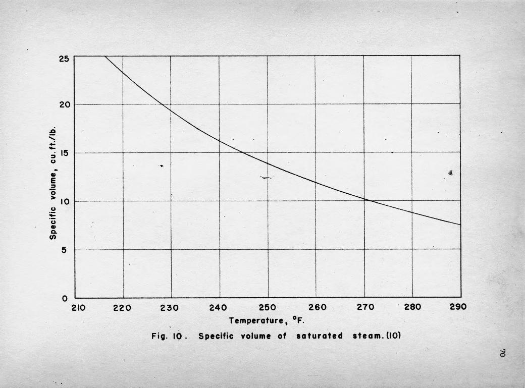
25

20

0 210 220 230 240 250 260 270 280 290

Temperature, °F.

Fig. 10 . Specific volume of saturated steam. (I0)

.01750

.01730

.01710

.01690

.01670

w.

.01650 210 220 230 240 250 260 270 280 290

Temperature, °F

Fig. II . Specific volume of saturated water. (10)

.0150

.0140

7; 0 C)

.0120

.0110

.0100 160 180 200 220 240 260 280 300

Temperature, °F.

Fig. 12 . Viscosity of saturated water vapor. (9)

.50

.40

0 .30 0 0 . _ 0 CL

C 0 0 20 ).... 4.-

0 V 0 5

. I 0

0

air

160 180 200 220 240 260 280 300 Temperature, °F.

Fig. 13. Viscosity of saturated water. (9)

d

46

42

38

34

30

26

22

18

14

74

160 180

200 220

240 260

280

Enthalpy,

btu/lb.

Fig.

14 .

Enthalpy

of various

saturation equilibrium

mixtures

of steam

and

water. (10)

1.000

.800

> .600 0

41x 12 13

.400

.200

0 0 10 20 30 40

Distance from pipe inlet, feet

Fig. 15. Graphical integration of test run number four.

A STUDY OF THE PRESSURE DROP ACCOMPANYING FLOA OF A FLASHING FLUID

IN A CIRCULAR PIPE

by

LEONARD PAUL GOLLOBIN

B. The City College of New York, 1951

ABSTRACT or THESIS

submitted in partial fulfillment of the

requirements tar the degree

MASTER OF SCIENCE

Department of Chemical Engineering

KANSAS STATE COLLEGE OF AGRICULTURE AND APPLIED SCIENCE

1952

2

AS. CT

An insulated pipe line which carries a vaporizing liquid and

receives no heat from an outside source is said to transport a flashing

old. Vaporization is the result of a decrease in the static pressure

satuwsted liquid due to frictional effects neemally easoeiated

ow through pipes, and is accompanied by a marked increase in the

linear velocity of the fluid stream because of the large volume of

vapor a asked.

tot)*

tared t

An energy ba

fl flow equations are not directly

LWOW. Pressure drops for this

stigation was to

equations could

about agy p pir ystem must account for

changes in the flow work term, kinetic energy, internal energy, and

potential energy of the flowing fluid, in addition to the week input

to or work done by the fluid, head input to or loss from the system,

and mechanical energy lost as a result of irreversible frictional

processes. Individual. terms of the mechanical energy balance are

expressed in terms of friction head, or pressure. The Fanning equation

and friction factor-Reynolds number correlation are commonly used to

estimate the frictional head, or pressure drop due to friction's effects.

The Fanning equation relates friction head to physical properties of the

flowing fluid and flow conditions existing in the pipe. When the fluid

properties or flow conditions vary along the pipe length, the equation

ferential feral

d(AP), iht0

dx 2gol),

where A is the friction pressure drop; dx, a differential secti0

of pipe; he Fanning fr cliea factor; Gf the mese velocity; ge, a

conversion constant; D, the inside diameter of the pipe; an the

density of the fluid, all terms being expressed in consistent units.

The Fanning friction factor, f, is expressed mathematically as follows*

(2) f ti) (B0) = 4)( )

The Fanning friction factor, f, is a function of the Re ynolds

number, e defined 'Oyaa, where D is the inside diameter of the pipe;

G, the mass velocity; and imp the viscosity of the fluid. Equation (2)

has been found to yield consistent results for oonaarcial pipes and

tubing. The only limitations surrounding application of the Fanning

equation and OtiO4 factor correlation are that steady state flow

exist and thet the pipe be, horizontal, round and running full of fluid.

The author has attempted to alter equations (1) end (2) to make them

applicable to the solution of flashing flow problems.

On the basis of published work for two,phase, two-component flow,

1 picture of the flow of 4 flashing fluid has been prOa inted.

o postulates that the liquid phase flows along the pipe

series of 'wings" and that the vapor phase flows as an

annulus, both phases riding on a liquid film which remains in contact

with the pipe wall and is in itself stationary.

Experimental measurements of the flow of flashing water-steam

mixtures were made in an insulated, horizontal three-eighths inch

schedule 40 galvanized iron pipe. Various methods of treating

the data were attempted in an effort to yield maculated friction heads

compatible with those observed. The most satisfactory results were

obtained by modifying the Fanning equation to account for vapor and

liquid flow contributions, to yield a combined friction head. The

relationships are expressed as follows:

1211 L dx J 00m. 2geD

(4) 4 " [Kg] L

(5) y PG(1

where the left-band term of equation (3) p reseats the combined

liquid and friction bead contributions quality or weight

percent of yap in the flowing fluid; end the subscripts V and L refer

to vapor and liquid phases respectiv04.

The limitations of the meth

problems are that

1. The investigation was 11

for analyzing a :ring flow

to the water -st tazn system.

2. The range of operating conditions observed was so velocity

from 73.5 to 133 lb./Isec.)(sq.ft.); inlet pressure, 27.7 to 42 paia.;

and ialat quality, Q, 0.026 to 1.95 percent.

Uses fated with the 7

torisoatal, PP271

of fluid..

or