A STUDY ON MHD JEFFERY-HAMEL FLOW IN NANOFLUIDS USING NEW HOMOTOPY ANALYSIS METHOD

International Journal of Scientific Research and Modern Education (IJSRME)

ISSN (Online): 2455 – 5630

(www.rdmodernresearch.com) Volume I, Issue I, 2016

15

A STUDY ON MHD JEFFERY-HAMEL FLOW IN NANOFLUIDS USING NEW HOMOTOPY

ANALYSIS METHOD Dr. V. Ananthaswamy* & N. Yogeswari**

* Assistant Professor, Department of Mathematics, The Madura College (Autonomous), Madurai, Tamilnadu

** M.Phil Scholar, Department of Mathematics, The Madura College (Autonomous), Madurai, Tamilnadu

Abstract: In this paper, the magnetic effect of nanofluids on the non-liner Jeffery-Hamel flow is investigated. The basic running equations which are strongly non-liner are solved analytically by using the New Homotopy analysis method. The analytical expression of the dimensionless velocity profiles are derived with the help of nanoparticle solid volume fraction, Hartmann number and Reynolds number by using the New HAM. Our analytical results are compared with the previous work (DTM) and a satisfactory agreement is noted. This method can be easily extended to solve the other non-linear initial and boundary value problem is fluids flow problem. Key Words: Jeffery-Hamel Flow, MHD, Nano Fluids, Differential Transformation Method & New Homotopy Analysis Method. 1. Introduction: The study of an incompressible viscous fluid flow through convergent-divergent channels is one of the most applicable fields such as fluid mechanics, civil environment, bio-mechanical engineering. This flow situation was initially introduced by Jeffery et al [4] and Hamel et al[3]. After some years, this problem was elaborately researched by various researchers. The theory of MHD is the study of the interaction between magnetic fields and moving conducting fluids. The Jeffery Hamel problem deals with other methods such as the Homotopy perturbation method (HAM), the Adomain decomposition method (ADM) and the Spectral- Homotopy analysis method. Earlier, these three analytical methods applied to find approximation analytical solution of Jeffery Hamel flow were used by Joneidi et al[5]. The description of theoretical part of this problem consulting with magnetic hydrodynamic (MHD) flows of viscous fluids have been performed before ten years due to their rapidly increasing applications in many fields of technology and engineering. Such applications include MHD power generation MHD flows meters and MHD pumps by Sutton et al[6]. One type of MHD problems is Jeffery Hamel problem. The third order non-linear ordinary differential equation describes this Jefferyet al [4] and Hamel et al [3] have studied this problem before Jeffery-Hamel flow is an exact similarity solution of the Navier-stokes equation in the special case of two dimensional flow through a channel with inclined plane walls meeting at a vortex and with a source or sink at the vortex by Moghimiet al [1]. Recently, the effect of magnetic field and nanoparticle on the Jeffery-Hamel flow using a powerful analytical method called Adomain decomposition method was studied by Sheikholeslami et al [2]. The aim of this problem is using by New Homotopy method to upshot the approximation solutions of running equation with the effect of nanoparticle volume fraction on velocity profiles. Considering aspects, the combined effect of nanoparticles and magnetic field to the relation among velocity field in the Jeffery-Hamel flow problem using Channel angle and Reynolds number in the flow using modified HAM is not addressed yet.


ISSN (Online): 2455 – 5630


16

2. Mathematical Formulation of the Problem: In this section, we study the steady fully developed flow of an incompressible conducting viscous fluid between two rigid plane walls that meet at an angle 2 as shown in Fig. 1. The rigid walls are considered to be divergent if 0 and convergent if

0 . We assume that the velocity is purely radial and depends on r and so that )0),,(( ruv only and further there is no magnetic field in the z-direction. The

following equation, the Navier -Stokes equation and Maxwell’s equations in polar coordinates are given below

0

r

)ru(

r

nf (1)

0111

2

2

0

2222

2

u

r

B

r

P

r

uu

r

uu

rr

u

rr

u

nfnfnf

nf

(2)

021

2

u

rnf

nf

nf

(3)

Here ),( ruu is the velocity, P is the pressure, 0B is the electromagnetic induction,

is the conductivity of the fluid, nf is the effective viscosity, nf is the effective density

and Knf is the effective thermal conductivity of nanofluid. The boundary conditions are

At the centerline of the channel: ,u

0

At the boundary of the channel: u=0.

Fig.1 Geometry of the MHD Jeffery-Hamel flow in convergent/divergent channel with

angle 2


ISSN (Online): 2455 – 5630


17

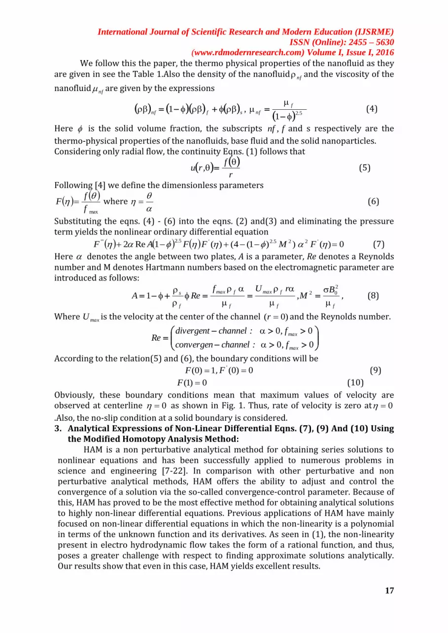
We follow this the paper, the thermo physical properties of the nanofluid as they are given in see the Table 1.Also the density of the nanofluid nf and the viscosity of the

nanofluid nf are given by the expressions

521

1.

f

nfsfnf ,

(4)

Here is the solid volume fraction, the subscripts fnf , and s respectively are the

thermo-physical properties of the nanofluids, base fluid and the solid nanoparticles. Considering only radial flow, the continuity Eqns. (1) follows that

r

f,ru

(5)

Following [4] we define the dimensionless parameters

maxf

fF

where

(6)

Substituting the eqns. (4) - (6) into the eqns. (2) and(3) and eliminating the pressure term yields the nonlinear ordinary differential equation

0)())1(4()(1Re2 '225.2'5.2''' FMFFAF (7)

Here denotes the angle between two plates, A is a parameter, Re denotes a Reynolds number and M denotes Hartmann numbers based on the electromagnetic parameter are introduced as follows:

ff

fmax

f

fmax

f

s BM,

rUfReA

2

021 , (8)

Where maxU is the velocity at the center of the channel )0( r and the Reynolds number.

00

00

max

max

f,:channelconvergen

f,:channeldivergentRe

According to the relation(5) and (6), the boundary conditions will be

1)0( F , 0)0(' F (9)

0)1( F (10)

Obviously, these boundary conditions mean that maximum values of velocity are observed at centerline 0 as shown in Fig. 1. Thus, rate of velocity is zero at 0

.Also, the no-slip condition at a solid boundary is considered. 3. Analytical Expressions of Non-Linear Differential Eqns. (7), (9) And (10) Using

the Modified Homotopy Analysis Method: HAM is a non perturbative analytical method for obtaining series solutions to nonlinear equations and has been successfully applied to numerous problems in science and engineering [7-22]. In comparison with other perturbative and non perturbative analytical methods, HAM offers the ability to adjust and control the convergence of a solution via the so-called convergence-control parameter. Because of this, HAM has proved to be the most effective method for obtaining analytical solutions to highly non-linear differential equations. Previous applications of HAM have mainly focused on non-linear differential equations in which the non-linearity is a polynomial in terms of the unknown function and its derivatives. As seen in (1), the non-linearity present in electro hydrodynamic flow takes the form of a rational function, and thus, poses a greater challenge with respect to finding approximate solutions analytically. Our results show that even in this case, HAM yields excellent results.


ISSN (Online): 2455 – 5630


18

Liao [7-15] proposed a powerful analytical method for non-linear problems, namely the Homotopy analysis method. This method provides an analytical solution in terms of an infinite power series. However, there is a practical need to evaluate this solution and to obtain numerical values from the infinite power series. In order to investigate the accuracy of the Homotopy analysis method (HAM) solution with a finite number of terms, the system of differential equations were solved. The Homotopy analysis method is a good technique comparing to another perturbation method. The Homotopy analysis method contains the auxiliary parameter h , which provides us with a simple way to adjust and control the convergence region of solution series. Using this method, we can obtain the following solution to (1) and (2) (see Appendix B).

uy

sk

kycos

kcos

k

k

kycos

k

ykcos

)k(cos

kh

kcos

ykcoskcos)y(F

218

22

12

1

2

2

2

222

1

(11)

Where, 225.25.2 )1(4)1(Re2 MAk (12)

5.2

1 )1(Re2 Ak (13)

225.2

2 )1(4 Mk (14)

2

2

222

1

2

2

222

1

1

)1(cos8

1cos2

)1(cos2

)1(cos

cos

8

2coscoscos2

)1(cos22

kk

k

kk

k

k

k

kk

kk

k

k

k

kk

k

k

s

(15)

2

2

222

1 1

)1(cos8

1cos2

)1(cos2 kk

k

kk

k

k

ku

(16)

4. Results and Discussion: In this section, Figure 1 shows that MHD Jeffery-Hamel flow in convergent/divergent channel with angle 2 .Figure (2)-(5) we discuss about the effect of the dimensionless velocity ))(( f versus the dimensionless angle )( with various

value of parameters MRe,, and .Figure 2 represents for some given fixed values of

MRe,, and .We observe that the fluidvelocity profiles decreases in divergent

channel. Figure 3(a) for some given fixed values of MRe,, and varying values of . We

infer that the solid volume fraction increases the fluid decreases. Figure 3 (b)

represents for some given fixed values of MRe,, and various values of . We noted

that the solid volume fraction increases the fluid decreases. That is, the fluid velocity

is more for base fluid and less for nanofluid. Figure 4 represents for some given fixed values of Re, and various values of ,M . It shows that the Hartmann number

increases the fluid velocity increases for both viscous and nanofluid. Figure 5 represents the for some given fixed values of M, and varying values of Re, . It evident that

Reynolds number increases the fluid velocity decreases for both viscous and nanofluid


ISSN (Online): 2455 – 5630


19

Fig.2: Dimensionless velocity )(f versus dimensionless angle ( ). The curve is plotted

for various values of the dimensionless parameters ,MRe,, using the eqn. (11)

with h=0.9.

Fig.3(a): Dimensionless velocity )(f versus dimensionless angle ( ). The curves are

plotted for various values of solid volume fraction ( ) and in some fixed values

of the other dimensionless parameters MRe,, using the eqn. (11) with h=

0.98.


ISSN (Online): 2455 – 5630


20

Fig.3(b): Dimensionless velocity )(f versus dimensionless angle ( ). The curves are

plotted for various values of solid volume fraction ( ) and in some fixed values

of the other dimensionless parameters MRe,, using the eqn. (11) with h=

0.97.

Fig.4: Dimensionless velocity )(f versus dimensionless angle ( ). The curves are

plotted for various values of solid volume fraction ( ), Hartmann number ( M )

and in some fixed values of the other dimensionless parameters Re, using the

eqn. (11) with h= 0.97.


ISSN (Online): 2455 – 5630


21


plotted for various values of solid volume fraction ( ), Reynolds number (Re)

and in some fixed values of the other dimensionless parameters M, using the

eqn. (11) with h=0.97.


plotted for various values of channel angle )( and in some fixed values of the

other dimensionless parameters ,MRe, using the eqn. (11) with h=0.975.


ISSN (Online): 2455 – 5630


22

Table 1: Comparison between DTM – NHAM solution for velocity profiles when .50,5,50Re,0 M and 44878.0h

NHAM DTM 0 1 1

0.1 0.996780 0.996756 0.2 0.986480 0.986491 0.3 0.967510 0.967516 0.4 0.936768 0.936738 0.5 0.889250 0.889208 0.6 0.817444 0.817461 0.7 0.710655 0.710623 0.8 0.553344 0.553388 0.9 0.325189 0.325142 1 0 0

Table 2: Comparison between DTM – NHAM solution for velocity profiles when.50,5.7,50Re,0 M and 6404.0h

NHAM DTM 0 1 1

0.1 0.993799 0.993761 0.2 0.974719 0.974790 0.3 0.942219 0.942283 0.4 0.894719 0.894750 0.5 0.829749 0.829759 0.6 0.743499 0.7434936 0.7 0.630049 0.630013 0.8 0.479936 0.479970 0.9 0.278370 0.278323 1 0 0

Table 3: Comparison between DTM – NHAM solution for velocity when 100,5,5Re,1.0 M and 935510.h

NHAM DTM 0 1 1

0.1 0.989400 0.989433 0.2 0.957800 0.957802 0.3 0.905320 0.905313 0.4 0.832320 0.832308 0.5 0.739250 0.739270 0.6 0.626860 0.626815 0.7 0.495692 0.495699 0.8 0.346880 0.346815 0.9 0.181171 0.181193 1 0 0

Table 4: Comparison between DTM – NHAM solution for velocity when 5,25Re,0 and 8736.0h

0M NHAM DTM


ISSN (Online): 2455 – 5630


23

0 1 1 0.1 0.986616 0.986669 0.2 0.947224 0.947251 0.3 0.883412 0.883404 0.4 0.797645 0.797674 0.5 0.693288 0.693202 0.6 0.573346 0.573389 0.7 0.441577 0.441558 0.8 0.360171 0.300645 0.9 0.152987 0.152962 1 0 0

500M NHAM DTM 0 1 1

0.1 0.990200 0.990221 0.2 0.960920 0.960939 0.3 0.912295 0.912287 0.4 0.844496 0.844405 0.5 0.757300 0.757317 0.6 0.650764 0.650758 0.7 0.523916 0.523953 0.8 0.375360 0.375331 0.9 0.202150 0.202153 1 0 0

Table 5: Comparison between DTM – NHAM solution for velocity when 5,25Re,2.0 and 98442.0h

0M NHAM DTM 0 1 1

0.1 0.984720 0.984743 0.2 0.939924 0.939943 0.3 0.868333 0.868370 0.4 0.774139 0.774186 0.5 0.662303 0.662374 0.6 0.538158 0.538121 0.7 0.406279 0.406256 0.8 0.360171 0.270828 0.9 0.134767 0.134828 1 0 0

200M NHAM DTM 0 1 1

0.1 0.986139 0.986132 0.2 0.945279 0.945255 0.3 0.879408 0.879425 0.4 0.791791 0.791774


ISSN (Online): 2455 – 5630


24

0.5 0.685999 0.686043 0.6 0.566091 0.566012 0.7 0.435127 0.435188 0.8 0.296639 0.296318 0.9 0.151119 0.151112 1 0 0

5. Conclusion: We conclude that, using New Homotopy method, the analytical approximation solution of MHD on Jeffery-Hamel flow problem in the nanofluid could be determined. The approximate analytical expression of the dimensionless velocity has been derived by using the New Homotopy analysis method. The HAM solution has been compared with the DTM solution. The obtained result is reliable and it leads to many applications of non-linear ordinary differential equations. We also discussed the influence of various physical parameters on velocity in detail. 6. Acknowledgement: Researchers express their gratitude to the secretary Shri. S. Natanagopal, Madura College Board, Madurai, Dr. K. M. Rajasekaean, The Principal and Dr. S. Muthukumar, Head of the Department of Mathematics, The Madura College (Autonomous), Madurai, Tamil Nadu, India for their constant support and encouragement. 7. References:

1. S.M. Moghimi, G. Domairry, Soheil Soleimani, E. Ghasemi, H. Bararnia, Application of homotopy analysis method to solve MHD Jeffery-Hamel flows in non-parallel walls, Advances in Engineering Software 42 (2011) 108-113.

2. M. Sheikholeslami, D.D. Ganji, H.R. Ashorynejad, H.B. Rokni, Analytical investigation of Jeffery-Hamel flow with high magnetic field and nanoparticle by Adomain decompositiom method, Appl. Math. Mech. Engl. Ed. 33 (2012) 25-36

3. G. Hamel, Spiralformige Bewgungen Zaher Flussigkeiten. Jahresber. Deutsch. Math. Verein. 25 (1916) 34-60.

4. G.B. Jeffery, The two-dimensional steady motion of a viscous fluid. Phil. Mag. 6 (1915) 455-465.

5. A.A. Joneidi, G. Domairry, M. Babaelahi, Three analytical methods applied to Jeffery-Hamel flow, Commun. Nonlinear Sci. Numer. Simulat. 15 (2010) 3423-3434.

6. G.W. Sutton, A. Sherman, Engineering Magneto hydrodynamics, McGraw-Hill, New York (1965).

7. S. J. Liao, The proposed homotopy analysis technique for the solution of non linear problems, Ph.D. Thesis, Shanghai Jiao Tong University, 1992.

8. S. J. Liao, An approximate solution technique which does not depend upon small parameters: a special example, Int. J. Non-Linear Mech. 30, pp.371-380, 1995.

9. S. J. Liao, Beyond perturbation introduction to the Homotopy analysis method, 1st edn. Chapman and Hall, CRC press, Boca Raton p.336, 2003.

10. S. J. Liao, On the Homotopy analysis method for nonlinear problems, Appl. Math. Comput. 147, pp. 499-513, 2004.

11. S. J. Liao, An optimal Homotopy-analysis approach for strongly nonlinear differential equations, Commun. Nonlinear Sci. Numer. Simulat. 15, pp. 2003-2016, 2010.

12. S. J. Liao, The Homotopy analysis method in nonlinear differential equations, Springer and Higher education press, 2012.


ISSN (Online): 2455 – 5630


25

13. S. J. Liao, An explicit totally analytic approximation of Blasius viscous flow problems. Int J. Nonlinear Mech; 34, pp. 759–78, 1999

14. S. J. Liao, On the analytic solution of magneto hydrodynamic flows non-Newtonian fluids over a stretching sheet. J Fluid Mech: 488, pp.189–212, 2003.

15. S. J. Liao, A new branch of boundary layer flows over a permeable stretching plate. Int J. Nonlinear Mech: 42, pp. 19–30, 2007.

16. G. Domairry, H. Bararnia, An approximation of the analytical solution of some nonlinear heat transfer equations: a survey by using Homotopy analysis method, Adv. Studies Theory Phys. 2, pp. 507-518, 2008.

17. Y. Tan , H. Xu , S.J. Liao, Explicit series solution of travelling waves with a front of Fisher equation. Chaos Solitons Fractals: 31, pp. 462–72, 2007.

18. S. Abbasbandy, Soliton solutions for the FitzhughNagumo equation with the homotopy analysis method. Appl Math Model: 32, pp.2706–14, 2008.

19. J. Cheng, S. J. Liao, R. N. Mohapatra, K. Vajravelu, Series solutions of nano boundary layer flows by means of the homotopy analysis method. J Math Anal Appl: 343, pp. 233–245, 2008.

20. T. Hayat, Z. Abbas , Heat transfer analysis on MHD flow of a second grade fluid in a channel with porous medium. Chaos Solitons Fractals: 38, pp.556–567, 2008.

21. T. Hayat, R. Naz, M. Sajid, On the homotopy solution for Poiseuille flow of a fourth grade fluid. Commun Nonlinear Sci Numer Simul: 15, pp. 581–589, 2010.

22. H. Jafari, C. Chun, S. M. Saeidy, Analytical solution for nonlinear gas dynamic Homotopy analysis method, Appl. Math. 4, pp.149-154, 2009.

23. M. Subha, V. Ananthaswamy and L. Rajendran, Analytical solution of non-linear boundary value problem for the electrohydrodynamic flow equation, International Jouranal of Automation and Control Engineering, 3(2), 48-56, (2014).

24. K. Saravanakumar, V. Ananthaswamy, M. Subha and L. Rajendran, Analytical Solution of nonlinear boundary value problem for in efficiency of convective straight Fins with temperature-dependent thermal conductivity, ISRN Thermodynamics, Article ID 282481, 1-18, (2013).

25. V. Ananthaswamy, M. Subha, Analytical expressions for exothermic explosions in a slab, International Journal of Research – Granthaalayah, 1(2), 2014, 22-37.

26. V. Ananthaswamy, S. Uma Maheswari, Analytical expression for the hydrodynamic fluid flow through a porous medium, International Journal of Automation and Control Engineering, 4(2), 2015, 67-76.

27. V. Ananthaswamy, L. Sahaya Amalraj, Thermal stability analysis of reactive hydromagnetic third-grade fluid using Homotopy analysis method, International Journal of Modern Mathematical Sciences, 14 (1), 2016, 25-41.

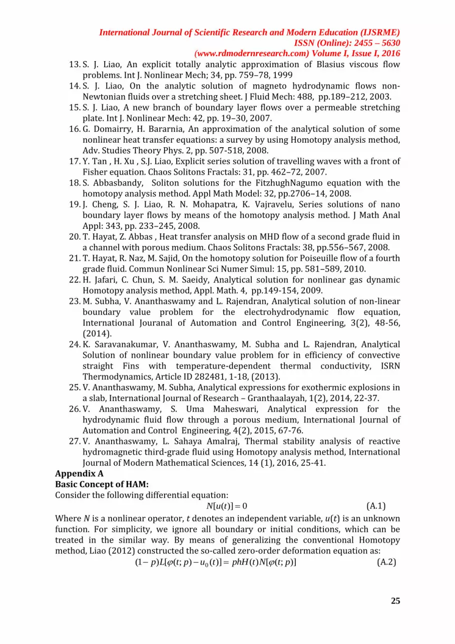
Appendix A

Basic Concept of HAM: Consider the following differential equation:

0)]([ tuN (A.1)

Where Ν is a nonlinear operator, t denotes an independent variable, u(t) is an unknown function. For simplicity, we ignore all boundary or initial conditions, which can be treated in the similar way. By means of generalizing the conventional Homotopy method, Liao (2012) constructed the so-called zero-order deformation equation as:

)];([)()]();([)1( 0 ptNtphHtuptLp (A.2)


ISSN (Online): 2455 – 5630


26

where p [0,1] is the embedding parameter, h ≠ 0 is a nonzero auxiliary parameter, H(t) ≠ 0 is an auxiliary function, L an auxiliary linear operator, 0u (t) is an initial guess of

u(t), ):( pt is an unknown function. It is important to note that one has great freedom

to choose auxiliary unknowns in HAM. Obviously, when 0p and 1p , it holds:

)()0;( 0 tut and )()1;( tut (A.3)

respectively. Thus, as p increases from 0 to 1, the solution );( pt varies from the initial

guess )(0 tu to the solution u (t). Expanding );( pt in Taylor series with respect to p, we

have:

1

0 )()();(m

mm ptutupt (A.4)

where

0

);(

!

1)(

pm

m

mp

pt

mtu

(A.5)

If the auxiliary linear operator, the initial guess, the auxiliary parameter h, and the auxiliary function are so properly chosen, the series (A.4) converges at p =1 then we have:

1

0 )()()(m

m tututu . (A.6)

Differentiating (A.2) for m times with respect to the embedding parameter p, and then setting p = 0 and finally dividing them by m!, we will have the so-called mth -order deformation equation as:

)()(][ 11

mmmmm uthHuuL (A.7)

where

1

1

1)];([

)!1(

1)(

m

m

mmp

ptN

mu

(A.8)

and

.1 1,

,1 ,0

m

mm (A.9)

Applying 1L on both side of eqn. (A7), we get

)]()([)()( 1

11

mmmmm utHhLtutu (A10)

In this way, it is easily to obtain mu for ,1m at thM order, we have

5r

M

m

m tutu0

)()(

(A.11)

When M , we get an accurate approximation of the original eqn.(A.1). For the convergence of the above method we refer the reader to Liao [20]. If an eqn. (A.1) admits unique solution, then this method will produce the unique solution. Appendix B Analytical Expressions of the Eqns. (7), (9) and (10) Using the New Modified Homotopy Analysis Method: In this appendix, we derive the analytical expressions for )(f using the HAM.


ISSN (Online): 2455 – 5630


27

The eqns. (7) can be written in the following form

01412 225252 )(F)M)(()(FFAReF '.'.''' (B.1)

We construct the homotopy for these equation as follows:

))(F)M)(()(F)(F)(ARe)(F((hp

))(F)M)(()(F)(F)(ARe)(F()p(

'.'.'''

'.'.'''

225252

225252

1412

140121

(B.2)

The approximate solution of the eqns. (B.2)is given by

...pp 2

2

10 (B.3)

The initial approximations are as follows:

010010 000 )(F,)(F,)(F' (B.4 (a))

......,,,i,)(F,)(F,)(F i

'

ii 321010000 (B. 4(b))

Substituting the eqn.(B.3) into an eqn. (B.2) we get

...))p(F)M)((

...)p(F...)(p(F)(ARe

...)p(F((hp...))p(F)M)((

...)p(F)(F)(ARe...)p(F()p(

'.

'.

''''.

'.'''

10

2252

1010

52

1010

2252

10

52

10

14

12

14

0121

(B.5)

Comparing the coefficients of like powers of p in eqn.(B.5), we get the following eqn.

01412 0

2252

0

52

0

0 )(F)M)(()(F)(ARe)(F:p '.'.''' (B.6)

01412

1412

0

2252

0

52

0

1

2252

1

52

1

1

))(F)M)((h)(F)(F)(AReh)(F(h

)(F)M)(()(F)(ARe)(F:p

'.'.'''

'.'.'''

(B.7)

Solving the eqns. (B.6), (B.7)and using boundary conditions (B.4), we obtained the following results:

10

kcos

ykcoskcos)y(F

(B.8)

uy

sk

kycos

kcos

k

k

kycos

k

ykcos

)k(cos

k)y(F

218

22

12

2

2

2

222

1

1

(B.9)

where, andskkk ,,, 21 u defined in the text eqns. (12)-(16) respectively.

According to the Homotopy analysis method we have

10

1FF)y(FlimF

p

(B.10)

Using the eqns. (B.8)and (B.9) into an eqn. (B.10), we obtain the solution in the text eqn. (11). Appendix C:

Table 1: Thermo- physical properties for pure water and copper nanoparticle.

Property Pure water Copper (cu)

)/( 2mkg 997.1 8933

)/( sNm 1 310 -

)/( mKW 0.613 400 )/1( K 207 610 17 610


ISSN (Online): 2455 – 5630


28

Appendix D: Nomenclature:

Symbol Meaning

Dimensionless angle

Solid volume fraction

Channel angle Re Reynolds number

M Hartmann number

)(f Dimensionless velocity

P Pressure

0B Electromagnetic induction

Conductivity

nf Effective viscosity

nf Effective density

nfK Effective thermal conductivity

Documents

A STUDY ON MHD JEFFERY-HAMEL FLOW IN NANOFLUIDS USING NEW HOMOTOPY ANALYSIS METHOD