A Temporal Query Language for OLAP: Implementation and a Case Study

A Temporal Query Language for OLAP:Implementation and a Case Study

Alejandro A. Vaisman1 and Alberto O. Mendelzon2

1 Universidad de Buenos [email protected]

2 University of [email protected]

Abstract. Commercial OLAP systems usually treat OLAP dimensionsas static entities. In practice, dimension updates are often necessary inorder to adapt the multidimensional database to changing requirements.In earlier work we proposed a temporal multidimensional model andTOLAP, a query language supporting it, accounting for dimension up-dates and schema evolution at a high level of abstraction. In this paperwe present our implementation of the model and the query language. Weshow how to translate a TOLAP program to SQL, and present a real-lifecase study, a medical center in Buenos Aires. We apply our implemen-tation to this case study in order to show how our approach can addressproblems that occur in real situations and that current non-temporalcommercial systems cannot deal with. We present results on query anddimension update performance, and briefly describe a visualization toolthat allows editing and running TOLAP queries, performing dimensionupdates, and browsing dimensions across time.

1 Introduction

In models for OLAP (On Line Analytical Processing) [7,2,9], data is representedas a set of dimensions and fact tables. Dimensions are usually organized ashierarchies, supporting different levels of data aggregation. We argued in earlierwork [5,6,10] that, although commercial OLAP tools largely do not supportupdates to dimension tables, these updates are likely to occur in many real-life situations. For instance, in Figure 1, a dimension Geography is representedas a hierarchy with levels city, province, region, country, and a distinguishedlevel All. A business decision may allow regions to be spread across differentcountries(which is not allowed in the dimension of Figure 1). This change maybe incorporated by deleting the edge joining the region and country levels, andadding a new edge from region to All.

Furthermore, thinking of a data warehouse as a materialized view of datalocated in multiple sources [14], it may happen that the structure of these sourceschanges, a new source is added, or an old one dropped. Any of these changesmay require updates to the structure of some dimensions.

In earlier work [10] we showed that in an evolving OLAP scenario like theabove, systems need temporal features to keep track of the different states of

G. Grahne and G. Ghelli (Eds.): DBPL 2001, LNCS 2397, pp. 78–96, 2002.c© Springer-Verlag Berlin Heidelberg 2002

A Temporal Query Language for OLAP 79

provinceOntario Mendoza

Toronto

region

country

All

city

Canada Argentina

East

all

San Juan

San Juan City San Rafael

Cuyo

Fig. 1. A Geography dimension

a data warehouse throughout its lifespan. We introduced the temporal multidi-mensional data model, and a temporal OLAP query language called TOLAP.We showed that TOLAP expresses typical OLAP queries in a concise and ele-gant fashion. Moreover, TOLAP fully supports schema evolution and versioning,unlike the best-known temporal query languages such as TSQL2, which onlysupports schema versioning in a limited way ([12], p.29).

In this paper we present our implementation of the model and the querylanguage. We show how to translate a TOLAP program to SQL and presenta real-life case study, using data from a medical center in Buenos Aires, Ar-gentina. We apply our implementation to this case study in order to show howour approach can address problems that occur in real situations and that currentnon-temporal commercial systems cannot deal with. We present results on queryand dimension update performance, and briefly describe a visualization tool thatallows editing and running TOLAP queries, performing dimension updates, andbrowsing dimensions across time.

Related WorkAs mentioned above, in previous work we argued that in practice one encoun-ters a wide range of possible dimension updates which the existing models fail tocapture. Kimball analyzes this problem to some degree [7], introducing the con-cept of slowly changing dimensions, which partially covers updates to dimensioninstances. Kimball suggests some partial solutions, like timestamping dimensiontuples with their validity intervals. This proposal neither takes schema versioninginto account, nor considers complex dimension updates.

Work carried out at the Time Center at the University of Arizona [1] analyzesthe performance of several SQL queries on three different implementations of anOLAP schema: “time series” fact tables, an “event” fact table, and dimensionstimestamped in the way proposed by Kimball. This work was, to our knowledge,the first to suggest an approach to temporal OLAP. Our work went further byproposing a model and a query language to address temporal issues at a higherlevel of abstraction.

80 Alejandro A. Vaisman and Alberto O. Mendelzon

More recently, a multidimensional model for handling complex data considersthe temporal aspect as a modeling issue [11], and addresses it in conjunction withother data modeling problems.

Paper Outline

The remainder of this paper is organized as follows: in Section 2 we review thetemporal multidimensional data model. In Section 3 we introduce the case study,along with a review of TOLAP based on examples over this case. In Section 4 wedescribe the implementation of the system. In Section 5 we show how a trans-lation of a TOLAP program to SQL proceeds. In Section 6 we present differenttests performed over the case study, discussing dimension update performance,expressiveness and visualization capabilities. We conclude in Section 7.

2 The Temporal Multidimensional Model

Due to space limitations we will introduce the Temporal Multidimensional Modelinformally and by an example. We refer to our previous work for full details [10].

2.1 Temporal Dimensions

In what follows, we will consider time as discrete; that is, a point in the time-line,called a time point, will correspond to an integer.

A temporal dimension schema is a directed acyclic graph where each noderepresents a level, and each edge is labeled with the time interval within whichthe edge was/is valid. At any instant t, the graph is a partial order with a uniquebottom level linf and a unique top level All.

Each dimension, at any time instant t, has an associated instance obtainedby mapping each level to a set of elements. For each pair of levels connected byan edge, an instance defines a function ρ called rollup, that maps the elements ofthe source level to the elements of the destination level. The rollup function fromlevel l1 to level l2 at instant t is denoted by ρ[t]l2l1 . Moreover, dimension instancesmust satisfy the consistency condition : at every instant t in the dimension’slifespan, for every pair of paths from one level to another, composing the rollupfunctions along the two paths yields identical functions.Notation: In the figures of this section, a label ti associated to an edge in agraph, will mean that the edge is valid for all t ≥ ti, and a label t∗i , that the edgewas valid for all t < ti. If an edge has no label, it is valid for all the dimension’slifespan.

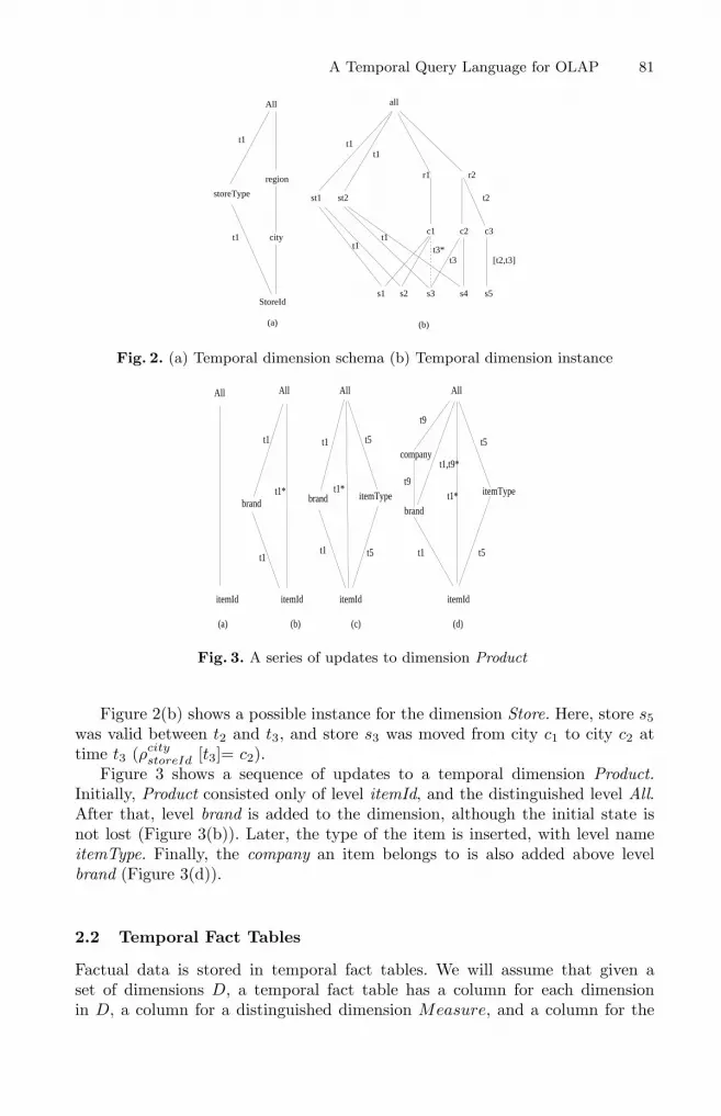
Example 1. Consider the dimension Store in Figure 2, with levels storeId, store-Type, city, region, and All. The figure depicts the history of this dimension asfollows: the initial levels were storeId, city, region and All. At time t1, level store-Type was added above storeId. As there is only one possible top level, an edgeis also added between storeType and All. This is called a Generalization [5].


All all

r1

StoreId

(a)

region

city

s1

(b)

s2 s4s3

r2

c2c1 c3

t2

s5

[t2,t3]

t1

t1

storeType st1 st2

t1t1

t1t1

t3*t3

Fig. 2. (a) Temporal dimension schema (b) Temporal dimension instance

itemId itemId

All

brand

itemType

company

t1

t9

t9

t5

t5

t1,t9*

t1*

(b) (c) (d)

itemId

All

(a)

brandt1*

t1

t1

All

t1

t1

brandt1*

All

itemType

t5

t5

itemId

Fig. 3. A series of updates to dimension Product

Figure 2(b) shows a possible instance for the dimension Store. Here, store s5was valid between t2 and t3, and store s3 was moved from city c1 to city c2 attime t3 (ρcity

storeId [t3]= c2).Figure 3 shows a sequence of updates to a temporal dimension Product.

Initially, Product consisted only of level itemId, and the distinguished level All.After that, level brand is added to the dimension, although the initial state isnot lost (Figure 3(b)). Later, the type of the item is inserted, with level nameitemType. Finally, the company an item belongs to is also added above levelbrand (Figure 3(d)).

2.2 Temporal Fact Tables

Factual data is stored in temporal fact tables. We will assume that given aset of dimensions D, a temporal fact table has a column for each dimensionin D, a column for a distinguished dimension Measure, and a column for the


Time dimension. A temporal base fact table is a temporal fact table such thatits levels are the bottom levels of each one of the dimensions in D (plus Measureand Time). As these bottom levels may vary during the lifespan of the datawarehouse, the schema of a base fact table can change. Keeping track of thedifferent versions of the fact tables is called, like in temporal database literature,schema versioning. Note, however, that the attributes in any column of a facttable always belong to the same dimension.

A Temporal Multidimensional Database is a set of temporal dimensions andtemporal fact tables.

Example 2. Given D = {Store, Product} where dimensions Store and Productare the ones of Figures 2 and 3 respectively, the temporal base fact table associ-ated to D would have levels {storeId, itemId, m, t}, where m is the measure andt is the time associated to a fact. If updates occur such that at time t12, brandbecomes the bottom level of dimension Product, the levels in the fact table willbe {storeId, brand, m, t}.

In temporal databases, in general, instances are represented using valid time,this is, the time when the fact being recorded became valid. On the contrary,a database schema holds within a time interval that can be different from theone within which this schema was valid in reality. Changes in the real worldare not reflected in the database until the database schema is updated. Schemaversioning, thus, is often related with transaction time. In the temporal multidi-mensional model we are describing, things are different than above. An updateto a dimension schema modifies the structure as well as the instance of thedimension. Figure 2 shows a dimension where schema and instance updates oc-curred. When storeId becomes generalized to storeType, the associated rollupsmust correspond to the instants in which they actually hold. Thus, we considerthat temporal dimensions are represented by valid time. It is straightforward toextend the model for supporting temporal dimensions with valid and transac-tion times. However, at the moment, our implementation supports valid time fordimensions.

Fact table instances can be represented using valid and transaction times,because the model supports user-defined time dimensions. In our implementa-tion, valid and transaction times for fact tables are supported through system-maintained and user-defined time attributes. In Subsection 2.3 we give an ex-ample of these kinds of time attributes. When a bottom level of a dimensionis deleted or a level is added below it, the schema of the associated fact tablesare modified, and new versions are created for them automatically. Thus, in ourimplementation, fact table versioning is represented using transaction time.

2.3 The Case Study: A Medical Data Warehouse

Throughout this paper we will refer to a real-life case study, a medical center inArgentina. We will use this example to illustrate the need for temporal manage-ment in OLAP. We used six months of data from medical procedures performed


on inpatients at the center. Each patient receives different services, including ra-diographies, electrocardiograms, medicine, disposable material, and so on. Theseservices are denoted “Procedures”. Data was taken from different tables in theclinic’s operational database. Figure 4 shows the final state of the dimensions.We will explain in Section 6 how we simulated a temporal environment in whichthese dimensions were created at different times.

speciality

All

(a)

doctorId procedureId

(b)

All

procType group

subgroup

All

patientId

yearOfBirth

yearRange

gender

institution

instType

(c)

Fig. 4. Dimensions in the case study

Dimension Procedure, with bottom level procedureId, and levels procedure-Type, subgroup and group, describes the different procedures available to patients.Dimension Patient, with bottom level patientId, and levels yearOfBirth and gen-der, represents information about the person under treatment. Age intervals arerepresented by a dimension level called yearRange. Patients are also groupedaccording to their health insurance institution. Moreover, these institutions arefurther grouped into types (level institutionType), such as private institutions,labor unions, etc. Dimension Doctor gives information about the available doc-tors (identified by doctorId) and their specialities (a level above doctorId). Thereis also a user-defined dimension Time, with levels day, week and month.

A fact table holds data about procedures delivered to patients by a certaindoctor on a certain date. We call this fact table Services, and its schema con-tains the bottom levels of the dimensions above, plus the measure. The fact ta-ble schema is : Services(doctorID,procedureId, patientID,day,quantity,t), wheret represents the system-maintained time dimension, and quantity is the mea-sure. For instance, a tuple <doc1,10.01.01,pat120,10,2,“10/10/2000”> meansthat doctor “doc1” prescribed two special radiographies to patient “pat120”on day “10” which corresponds to October 10th, 2001. In this case study, thesystem-maintained and user-defined times are synchronized, meaning that thereis a correspondence between the values of attributes “day” and “t”(e.g., day“11” corresponds to October 11st, 2000). This synchronization, however, is notmandatory in the model. Thus, both times can take independent values.


3 TOLAP

In this section we describe the temporal OLAP language TOLAP (Tempo-ral OLAP) [10]. TOLAP combines some of the features of temporal querylanguages like TSQL2 or SQL/TP [12,13] with some of the high-order featuresof languages like HiLog or SchemaLog [4,8], in an OLAP setting. We highlightTOLAP ’s main characteristics by means of examples, using the schema of themedical center described in the previous section .

TOLAP is a rule-based language; as in Datalog, each rule defines the pred-icate in the head using the literals in the body. It would be easy to give anSQL-like syntax to the language, but we find the rule-based syntax clearer andmore concise.

We begin our description of TOLAP with queries not involving aggregates.A query returning the procedures delivered to patients affiliated to unions willbe expressed in TOLAP as:

SrvU(proc,pat,qty,t)←− Services(doc,proc,pat,day,qty,t),pat[t]→insType:‘Union’;

This query returns a projection of the tuples in Services such that pat rolledup to ‘Union’ when the service was delivered. Variable pat represents an elementin the lowest level of the dimension Patient. A tuple in Services will contributeto the result if a patient pat was served by doctor doc on day day at time t,and pat was affiliated to an institution of type ‘Union’ at the time of beingtreated. The expression pat[t]→insType:‘Union’ is called a rollup atom, andServices(doc,proc,pat,day,qty,t) is a fact atom.

Queries with aggregates can readily be expressed in TOLAP. For example,consider the query: “total number of services per procedure type and week.”

SP(ty,w,SUM(qty))←− Services(doc,proc,pat,day,qty,t),proc[t]→procType:ty, day→week:w;

Descriptive attributes of dimension levels can be used in TOLAP queries.Suppose we want the total number of services delivered by Dr. Roberts eachweek. In TOLAP :

SB(w,SUM(qty))←− Services(doc,proc,pat,day,qty,t),day→week:w,doc[t]→doctorId:dr, dr.name=‘Roberts’;

The rollup function represented by the rollup atom doc[t]→doctorId:drwill be the identity during the intervals in which doctorId is the dimension’s bot-tom level. Thus, the atom doc[t]→doctorId:dr allows defining the attributename as an attribute of the level doctorId, no matter the location of this levelwithin the dimension’s hierarchy. The expression dr.name=‘Roberts’ is calleda descriptive atom.


TOLAP also allows querying the metadata, supporting queries with no facttable in the body of the rules, which we call metaqueries. For example: “List theperiods during which no heart surgery was available.”

NoHeart(t)←− !Procedure:procId:proc[t]→group:g,g.desc=‘Heart Surgery’.

The term !Procedure:procId:proc[t] is a negated rollup atom. Note thatwe must specify the name of the dimension and level for variable proc in theatom Procedure:procId:proc[t]→group:g, because there is no fact table inthe body of the rule to which proc could be bound.

As in Datalog, rules can be composed into programs. For example: “patientswho were administered procedures belonging to types delivered more than onehundred times.” We first compute the total number of procedures by type, anduse the result in the final query.

PT(ty,COUNT(qty))←− Services(doc,proc,pat,day,qty,t),proc[t]→procType:ty;

Q(pat)←− Services(doc,proc,pat,day,qty,t), q ≥ 100,Ty100(ty,q), proc[t]→procType[t]:ty;

The expression q ≥ 100 is called a constraint atom.

4 Implementation

The system was implemented on an ORACLE 8.04 database. The parser andvisual interfaces were written in Java using Borland’s Java Builder. Dimensionupdates were implemented as ORACLE’s PL-SQL stored procedures and func-tions.

Two different data structures were considered for representing dimensions: a“fixed schema” versus a “non-fixed schema” approach. In both of them, a relationwith schema of the form (dimensionId, loLevel, toLevel, From, To) representsthe structure of the dimensions in the data warehouse across time. A tuple inthis relation means that in the dimension identified by dimensionId, level loLevelrolled up to level toLevel between instants From and to. For example, the schemaof the data warehouse introduced in Section 2 will be represented by a relationwith tuples < D1, procedureId, procedureType, t1, Now >, < D1, procedureId,group, t2, Now >, < D1, group, subgroup, t5, Now >, and so on.

We briefly discuss how instances of the dimensions are stored under eachkind of representations.

Fixed Schema. Each dimension instance is represented by a relation withschema (loLevel,upLevel,loVal,upVal,From,To). Each tuple in this relation rep-resents a rollup ρupLevel

loLevel [(From, To)](loV al) = upV al. As an example, the in-stances of dimension Procedure of Section 3, would be represented by a rela-tion with tuples of the form < procedureId, procedureType, pr1, ty1, t1, t3 >,


< procedureId, subgroup, pr1, sg1, t2, t3 >, and so on. Thus, as new levels areadded to the dimension, new tuples are inserted,but the relation’s schema doesnot change. For instance, adding a new level priceRange above procedureId im-plies adding tuples like < procedureId, priceRange, pr1, 200to300, t6, Now > .

In this representation, dimension updates can be easily implemented, exceptupdates that add or delete edges between levels, called Relate and Unrelaterespectively [5,6]. These updates require self-joining the relation, in order tocheck consistency. Moreover, translation to SQL would be awkward, and theresulting SQL queries would require, again, self-joining temporal relations, asseen in the first SQL example below. In fact, self-joining temporal relations willbe necessary each time the transitive closure of the rollup functions must becomputed.

Non-fixed Schema. In this case there is also one relation for each dimension,but each dimension level is mapped to an attribute in this relation. A singletuple captures all the possible paths from an element in the bottom level, to thedistinguished element “all”. Two attributes, From and To, indicate, as usual inthe temporal database field, the interval within which a tuple is valid. For exam-ple, a relation representing dimension Procedure will have schema: {procedureId,procedureType, group, subgroup, From, To}.

This structure requires more complicated algorithms for supporting dimen-sion updates. For instance, adding a dimension level above a given one (general-ization), or below the bottom level(specialization), induces a schema update ofthe relation representing the dimension instance: a new column will be added tothis relation. If a level is deleted, no schema update occurs (i.e., the correspond-ing column is not dropped), in order to preserve the dimension’s history. In theexample above, a column priceRange would be added. However, the translationprocess is simpler, and the subsequent query performance better, because com-puting the transitive closure of the rollup functions reduces to a single relationscan.

To make these ideas more concrete, let us show how a TOLAP query istranslated to SQL in each approach. (In Section 5 we give more details of thistranslation process.) Consider the query “total procedures by group.” This queryreads in TOLAP :

GTot(g,SUM(qty))←−Services(doc,proc,pat,day,qty,t), proc[t] → group:g;

Assuming that no schema update affected the fact table Services, the SQLequivalent of the TOLAP query above in the fixed schema approach will looklike (for the sake of clarity we do not show here how time granularity is handledin the translation):

SELECT P1.upLevel,SUM(quantity)FROM Services S, Procedure P, Procedure P1, Time TWHERE


S.procedureId = P.loVal AND P.loLevel = ’procedureId’ ANDP.upLevel = P1.loLevel AND P.upLevel = ’subgroup’ ANDP1.upLevel = ’group’ ANDS.time BETWEEN P.From AND P.To ANDS.time BETWEEN P1.From AND P1.To

GROUP BY P1.upLevel

In the non-fixed schema representation, the SQL equivalent for the query is:

SELECT P.group,SUM(quantity)FROM Services S, Procedure PWHERES.procedureId = P.procedureId AND S.time BETWEEN P.From AND P.To

GROUP BY P.subgroup

Notice that computing the rollup from procedureId and group is straightfor-ward, while in the first approach the self-join of the table Procedure is required.

These arguments led us to choose the non-fixed schema approach for ourTOLAP implementation.

5 Translating TOLAP into SQL

The user interacts with the system through a visual interface. A dimensionupdate module, a TOLAP parser and a TOLAP translator access the databasethrough a JDBC driver. The TOLAP translator translates each atom into anSQL statement and builds the equivalent SQL query. We will show how a TOLAPrule of the form

Q(x,y,Ag(m)) ←− F(xi,yj,m,t), xi[t]→li:x, yj[Now]→lj:y, Dim:l:r[t]→p:z;

is translated to SQL. We assume that xi is bound to a dimension Di and yj

to dimension Dj . Also, m represents the measure of the fact table F.

5.1 Translating TOLAP Atoms

– For each rollup atom like xi[t] → li:x, a selection clause is built as follows:F.i = Dimi.bottom AND F.time BETWEEN Dimi.From AND Dimi.To

Dimension Dimi is the table representing the dimension Di. The first con-junct joins this dimension to the fact table on the attribute representing thebottom level. The actual name of the column F.i is taken from the facttable’s metadata. The second conjunct corresponds to the join between thefact table and the “Time” dimension.

– Each time constant is translated to a selection clause. The second rollupatom in the rule above will be translated as1:F.j = Dimj .bottom AND Dimj .To = Now

1 In an actual implementation, Now can be replaced by Sysdate() or any functionreturning the current time.


– A rollup atom Dim:l:r[t] → p:z, not bound to any fact table, is trans-lated as an EXISTS clause.

EXISTS(SELECT *FROM DimWHEREF.Time BETWEEN Dim.From AND Dim.To)

The WHERE clause is omitted if the join with the time dimension is not re-quired.

– If the rollup atom x → Y:x corresponds to a user-defined time dimension,the atom is translated asF.j = Dimj .bottom

– A constraint atom of the form x {<,=} C, where C is a constant term, istranslated as a selection condition in the WHERE clause. If the constraintatom is negated this condition is treated in the usual way (a NOT predicateis added).

– A negated rollup atom is translated as a NOT EXISTS clause. Suppose thatin the query above we add the negated atom!(yj[Now] → l1 :‘a’), where ‘a’ represents a constant. This atom is con-verted into an SQL expression of the form:

NOT EXISTS(SELECT *FROM Dimj

WHEREDimj .To=Now AND Dimj .l1 =‘a’ AND F.j = Dimj .bottom)

where l1 is the attribute representing level l1. A negated descriptive atom istranslated analogously.

– A predicate atom is translated as a table in the FROM clause, with the condi-tions which arise from the variables or constants in it.

5.2 TOLAP Rules

So far we tackled the problem of translating each atom in a TOLAP rule sep-arately. Now we will explain the translation of the whole rule. We put all thepieces of the WHERE clause together and use aggregation and projection forthe rollup from the bottom levels of the dimensions Di and Dj to the levels liand lj in the head of the clause. Thus, the SQL query generated by the TOLAPquery above will look like this:

SELECT Dimi.li, Dimj .lj,Ag(measure)FROM F 1, Dimi, Dimj

WHERE


F 1.i = Dimi.bottom AND F 1.j = Dimj .bottom ANDF 1.time BETWEEN Dimi.From AND Dimi.To AND Dimj .To = Now ANDEXISTS(SELECT *FROM DimWHEREF 1.Time BETWEEN Dim.From AND Dim.To )

GROUP BY Dimi.li, Dimj .lj

The term measure is the measure in the fact table, bound to variable m. Thefact table subindex represents the version of the fact table. So far there is onlyone version, as no schema update has occurred yet. However, we claimed that oneof the main TOLAP features is the ability to deal with schema updates triggeredby an specialization or a deletion of a bottom level. In the system’s catalog, ina table describing fact table data, a new tuple is stored each time a dimensionupdate affects a fact table in the data warehouse. Thus, given a fact table F , thisfact table may have versions F 1, F 2 and so on, with different schemas. Given aTOLAP rule Γ with a fact table F in the body, the SQL query Q equivalent toΓ will be such that Q = Q1 ∪Q2 ∪ . . . ∪Qn, where Qi are the queries involvingfacts occurred in the intervals Ii in which each F i holds. If the query includesan aggregate function, call it fAGG, one more aggregation must be performed,in order to consider duplicates in each subquery. Thus, QAGG = fAGG(Q)

Finally, TOLAP programs are compiled by translating each rule, creatingtemporary tables for each predicate in the head of a rule.

5.3 Join Elimination

There are cases in which the join between dimensions and fact tables is notneeded. This situation arises when a variable in the head of the rule is bound tothe bottom level of a fact table in the body, or to a level that was the bottomlevel at least during some interval Ii. Our implementation takes advantage ofthis fact, and does not generate the join.

Example 3. Let us consider the query “total procedures by procedureId and doc-tor speciality”. Assume that the fact table Services was split into Services 1 andServices 2, holding before and after a time instant t5 respectively. In Services 1,the levels procedureId and speciality were the bottom levels corresponding to thedimensions Procedure and Doctor. In Services 2, these bottom levels were pro-cedureId and doctorId. The query in TOLAP, and its SQL equivalent are:

PS(pro,sp,SUM(qty))←− Services(doc,prac,pat,day,qty,t),doc[t]→speciality:sp,prac[t]→procedureId:pro;

SELECT procedureId,speciality,SUM(quantity)FROM (

SELECT procedureId,speciality, SUM(quantity)


FROM Services 1GROUP BY procedureId,specialityUNION ALLSELECT procedureId,speciality, SUM(quantity)FROM Services 2, DoctorWHEREServices 2.Time BETWEEN Doctor.From AND Doctor.To ANDServices 2.doctorId=Doctor.doctorIdGROUP BY procedureId,speciality )

GROUP BY procedureId,speciality

Notice that, as speciality and procedureId were the bottom levels ofServices 1, no join is needed in the first subquery.

5.4 Subquery Pruning

If a TOLAP rule contains a constraint atom with a condition over time such thatthe lifespan of some version of the fact table does not intersect with the intervaldetermined by the constraint, the subquery corresponding to that version of thefact table is not generated by the translator, as it will not yield any tuple in theoutput. For instance, in Example 3, adding the constraint t < d6 will preventthe first subquery from being generated.

5.5 Translating to TSQL2

Although at first sight TSQL2 might appear as the obvious target for translatingTOLAP queries into an SQL-like query language, a more detailed analysis willshow some drawbacks of this approach. In what follows we will assume that thereader is familiar with the design of TSQL2 [12].

TSQL2 has an implicit time data model. This feature, although useful forqueries involving temporal joins, makes it difficult to express queries like theones we deal with here. This is related to the problem of lack of universality ofTQSL2, as studied by Chen and Zaniolo [3].

Although for some queries using TSQL2 would reduce or eliminate the needfor complex expressions involving time, most of the time these expressions do notactually affect performance. Moreover, explicit time management makes TOLAPsemantics easy to capture, whereas implicit time management turns this taskdifficult. For example, in TSQL2 the join of valid time relations returns anothervalid time relation. In order to avoid this behavior, different constructions mustbe used, for example the SNAPSHOT statement, which produces a non-temporalrelation. Granularities must be explicitly handled using the CAST construct, oftencombined with PERIOD and other operators like INTERSECT or CONTAINS. Thus,although aparently simpler, the generated code contains many TSQL2 keywords,reducing portability and delivering no benefit, as TOLAP already hides all timemanagement from the user.


For an example, consider the query:“total number of procedures by proce-dure subgroup and institution type” (we will be using this query for measuringperformance later in Section 6):

Q(b,c,SUM(qty))←− Services(doc,prac,pat,day,qty,t),prac[t]→subgroup:c, pat[t]→institutionType:b;

For the sake of simplicity we will assume that there is only one fact tableversion. In TSQL2, this query would read (in bold we indicate the TSQL2 key-words):

SELECT SNAPSHOT COL 0, COL 1, SUM(SUM 2)FROM (

SELECT SNAPSHOT DIMENSION PROCEDURE.subgroup AS COL 0,DIMENSION PATIENT.instType AS COL 1,SUM(QUANTITY) AS SUM 2FROM SERVICES 1, DIMENSION PATIENT, DIMENSION PROCEDUREWHERE VALID(DIMENSION PATIENT) CONTAINS VALID(SERVICES 1)AND SERVICES 1.PATIENTID = DIMENSION PATIENT.PATIENTID ANDVALID(DIMENSION PROCEDURE) CONTAINS VALID(SERVICES 1)AND SERVICES 1.PROCID = DIMENSION PROCEDURE.PROCIDGROUP BY DIMENSION PATIENT.INSTTYPE,DIMENSION PROCEDURE.SUBGROUP)

GROUP BY COL 0, COL 1

As TOLAP allows considering different instants for rollup evaluation, evenusing TSQL2 as the target language cannot prevent explicit time management.Suppose the query above is replaced by:

Q(b,c,SUM(qty))←− Services(doc,prac,pat,day,qty,t),proc[Now]→subgroup:c,pat[‘‘10/10/2000’’]→institutionType:b;

In this case, since the granularities of the arguments of the rollup functionsand the dimensions differ, the translator must also generate the TSQL2 state-ments for casting these differences.

For the translation above, we assumed that the fact table was created asan EVENT relation, and the dimension tables as STATE relations. However, theseassumptions carry further problems: as update semantics for TSQL2 is differentthan the semantics of dimension updates, ad-hoc modifications are needed tomake the translation work. This would be much more expensive than generatingthe SQL expressions for explicit time management. Another problem would bethe limited support provided by TSQL2 for schema versioning.

From the above we conclude that the benefits of translating TOLAP toTSQL2 are outweighed by the problems involved in adapting TSQL2’s semanticsto the semantics of TOLAP.


6 The Medical Clinic Case Study

In this section we apply the temporal approach to the case study introduced inSection 2.3. Our temporal multidimensional data model lets us not only modifythe dimensions on-line, but keep track of the history of the medical data ware-house. We will present a simulated scenario based on real data extracted fromthe system described in Section 2.3.

The objective of the study was to test the ability of the temporal approachand TOLAP to address user needs more fully than commercially available non-temporal OLAP tools. Using our implementation, we wanted to study: (a) perfor-mance, by measuring response time of dimension updates and TOLAP queries;(b) expressive power and abstraction, by posing queries which could not be easilyexpressed in non-temporal environments and comparing them with their SQLequivalent; and (c) visualization capabilities, through a graphical environmentthat supports browsing dimensions and fact tables across time, updating dimen-sions, and temporal querying of the warehouse.

6.1 Data Preparation

The testing scenario was prepared applying the following dimension updates.Dimension Procedure was created with bottom level procedureId. Subsequentoperations performed using the graphic interface generalized this level to levelsubgroup. Level procedureId was then generalized to procType. Finally, subgroupwas generalized to group, and procType related to group. (See Section 2.3 forexplanations of these and all other dimension levels mentioned in this section).In the Patient dimension, the initial bottom level patientId represents infor-mation about the person under treatment. This level was then generalized toyearOfBirth, gender and institution, in that order. Levels yearOfBirth and insti-tution were further generalized into yearRange and institutionType respectively.For dimension Doctor, in order to show how schema versioning is handled inTOLAP, we assumed that although facts were recorded at the doctorId level,this level was temporarily deleted, originating the second version of the fact ta-ble, called Services 2. Thus, during a short interval, the dimension’s bottomlevel was speciality, later specialized into level doctorId, which triggered the cre-ation of the third version of the fact table, denoted Services 3. Finally, a user-defined Time dimension was created, with granularity day, allowing expressingaggregates over time. The dimension’s hierarchy is the following: day rolls upto week and month; week and month roll up to All. The three resulting facttable versions have the following schemas: (a) Services 1:{procId, patientId,doctorId, day, quantity, tmp}, where tmp represents the built-in time dimension,and quantity is the number of procedures delivered; (b) Services 2:{procId,patientId, speciality, day, quantity, tmp}; (c) Services 3:{procId, patientId,doctorId, day, quantity, tmp}. The fact tables were populated off-line.

The following table depicts the number of tuples in each table of the rela-tional representation, after all the updates above ocurred.


Table # of tuplesPatient 16383

Procedure 11253Doctor 822Time 730

Services 1 26040Services 2 12464Services 3 17828

We also performed several updates at the instance level, simulating situa-tions where new doctors were hired, others left, new procedures were created, orpatients moved from one institution to another.

The tests were run on a PC with an Intel Pentium III 600Mhz processor, with128 Mb of RAM memory and a 9Gb SCSI Hard Disk. The Database ManagementSystem was an ORACLE 8.04 database running on top of a Windows NT 4(Service Pack 5) Operating System.

6.2 Discussion of Results

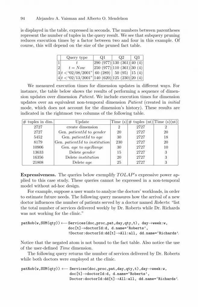
Performance. Figure 5 shows one of sets of TOLAP queries we ran. QueryQ1 has three rollup atoms in the body, while query Q3 has only one. We alsoran the three queries replacing variable t by the constant Now (i.e., the currentvalues of the rollups are considered for aggregation instead of the values holdingat the time of the service, see [10] for details).

Q1: Q(a,b,c,SUM(qty)) ←− Services(doc,proc,pat,day,qty,t),doc[t]→speciality:a, proc[t]→subgroup:c,pat[t]→institutionType:b ;

Q2: Q(b,c,SUM(qty)) ←− Services(doc,proc,pat,day,qty,t),proc[t]→subgroup:c, pat[t]→institutionType:b;

Q3: Q(b,SUM(qty)) ←− Services(doc,proc,pat,day,qty,t),pat[t]→institutionType:b;

Fig. 5. Queries

Finally, we included a constraint atom in the three queries, to see the influ-ence of the subquery pruning step. The constraint t <‘‘02/08/2001’’ leaves outfact tables Services 2 and Services 3, while the constraint t <‘‘02/13/2001’’leaves out fact table Services 3. For instance, query Q3 was modified as follows:

Q(b,SUM(qty))←− Services(doc,proc,pat,day,qty,t),pat[t]→institutionType:b, t <‘‘02/13/2001’’ ;

The table below shows the query execution times for the three sets of queriesdescribed above. Each query was ran three times, and the average response time


is displayed in the table, expressed in seconds. The numbers between parenthesesrepresent the number of tuples in the query result. We see that subquery pruningreduces execution times by a factor between two and four in this example. Ofcourse, this will depend on the size of the pruned fact table.

Query type Q1 Q2 Q31 t 290 (977) 130 (361) 40 (4)2 t = Now 250 (977) 110 (361) 30 (4)3 t <“02/08/2001” 60 (289) 50 (95) 15 (4)4 t <“02/13/2001” 140 (620) 125 (230) 20 (4)

We measured execution times for dimension updates in different ways. Forinstance, the table below shows the results of performing a sequence of dimen-sion updates over dimension Patient. We include execution times for dimensionupdates over an equivalent non-temporal dimension Patient (created in initialmode, which does not account for the dimension’s history). These results areindicated in the rightmost two columns of the following table.

# tuples in dim. Update Time (s) # tuples (nt) Time (s)(nt)2727 create dimension 2 2727 22727 Gen. patientId to gender 20 2727 205452 Gen. patientId to age 30 2727 188179 Gen. patientId to institution 230 2727 2010906 Gen. age to ageRange 30 2727 1013633 Delete gender 15 2727 316356 Delete institution 20 2727 321808 Delete age 25 2727 3

Expressiveness. The queries below exemplify TOLAP ’s expressive power ap-plied to this case study. These queries cannot be expressed in a non-temporalmodel without ad-hoc design.

For example, suppose a user wants to analyze the doctors’ workloads, in orderto estimate future needs. The following query measures how the arrival of a newdoctor influences the number of patients served by a doctor named Roberts: “listthe total number of services delivered weekly by Dr. Roberts while Dr. Richardswas not working for the clinic.”

patRob(w,SUM(qty))←−Services(doc,proc,pat,day,qty,t), day→week:w,doc[t]→doctorId:d, d.name=‘Roberts’,!Doctor:doctorId:dd[t]→All:all, dd.name=‘Richards’.

Notice that the negated atom is not bound to the fact table. Also notice the useof the user-defined Time dimension.

The following query returns the number of services delivered by Dr. Robertswhile both doctors were employed at the clinic.

patRob(w,SUM(qty)) ←− Services(doc,proc,pat,day,qty,t),day→week:w,doc[t]→doctorId:d, d.name=‘Roberts’,Doctor:doctorId:dd[t]→All:all, dd.name=‘Richards’.


The next query illustrates how to check patients who were served when theywere affiliated to ‘MEDICUS’ and are currently affiliated to ‘OSDE’.

changePlan(pat)←− Services(doc,proc,pat,day,m,t),pat[t]→institution:‘MEDICUS’,pat[Now]→institution:‘OSDE’.

Visualization Capabilities. The third goal of our experiments consisted inexercising on this case study the graphical environment we developed to supportthe temporal multidimensional model. We used this environment to perform thedimension updates reported above and to browse the structures and instancesof the dimensions across time, in order to test usefulness and performance ofthe tool. The graphic interface supports: (a) Browsing dimensions and instancesacross time, and seeing how they were hierarchically organized throughout theirlifespan. (b) Performing dimension updates (c) Importing rollup functions fromtext files. (d) Browsing different versions of a fact table. (e) Sending TOLAPprograms to the query engine, and displaying they results without leaving theenvironment, including the possibility to see the generated SQL query.

7 Conclusion and Future Work

We have described the implementation of TOLAP, a temporal OLAP querylanguage introduced in a previous work [10]. We discussed two different relationalrepresentation alternatives, and gave details of the translation from TOLAP toSQL, or program, showing that a query that is concisely expressed in TOLAPtakes many lines of complex SQL code. Finally, we tested our implementationon a real-life case study. Our preliminary results on query and dimension updateperformance suggest that TOLAP can be useful for overriding the limitations ofnon-temporal OLAP commercial tools.

Many research directions remain open. Query optimization in TOLAP isan obvious one. Also, TOLAP can be extended to allow the definition ofintegrity constraints, which could be easily introduced within our visualizationtool. Another issue deserving attention is adding update support to TOLAP,allowing bulk updates like “delete all customers who have not completed anytransaction since 1998.” Transactions in update expressions in TOLAP could bealso addressed. For example, the expression above may be followed by: “classifyall customers who did not perform any transaction since 1999 as ‘low prioritycustomers’ ”.

Acknowledgements

The authors wish to thank Daniel Grippo and Claudio Tirelli, at the Universityof Buenos Aires for their help with the implementation of TOLAP.

This work was partially supported by the Natural Sciences and EngineeringResearch Council of Canada, and by the FOMEC program for the University ofBuenos Aires.


References

1. R. Bliujute, S. Saltenis, G. Slivinskas, and G. Jensen. Systematic change man-agement in dimensional data warehousing. Time Center Technical Report TR-23,1998.

2. L. Cabibbo and R. Torlone. A logical approach to multidimensional databases. InEDBT’98: 6th International Conference on Exteding Database Technology, pages253–269, Valencia, Spain, 1998.

3. C.X. Chen and C. Zaniolo. Universal temporal extesions for database languages.In Proceedings of IEEE/ICDE’99, Sydney, Australia, 1999.

4. W. Chen, M. Kifer, and D.S. Warren. Hilog as a platform for database language.In Proceedings of the 2nd. International Workshop on Database Programming Lan-guages, pages 315–329, Oregon Coast, Oregon, USA, 1989.

5. C. Hurtado, A.O. Mendelzon, and A. Vaisman. Maintaining data cubes underdimension updates. Proceedings of IEEE/ICDE’99, 1999.

6. C. Hurtado, A.O. Mendelzon, and A. Vaisman. Updating OLAP dimensions. Pro-ceedings of ACM DOLAP’99, 1999.

7. R. Kimball. The Data Warehouse Toolkit. J.Wiley and Sons, Inc, 1996.8. L.V.S Lakshmanan, F. Sadri, and I.N. Subramanian. Logic and algebraic languages

for interoperability in multidatabase systems. Journal of Logic Programming 33(2),pp.101–149, 1997.

9. W. Lehner. Modeling large OLAP scenarios. In EDBT’98: 6th International Con-ference on Exteding Database Technology, Valencia, Spain, 1998.

10. A.O. Mendelzon and A. Vaisman. Temporal queries in OLAP. In Proceedings ofthe 26th VLDB Conference, Cairo, Egypt, 2000.

11. T.B Pedersen and C. Jensen. Multidimensional data modeling for complex data.Proceedings of IEEE/ICDE’99, 1999.

12. Richard Snodgrass. The TSQL2 Temporal Query Language. Kluwer Academic Pub-lishers, 1995.

13. D. Toman. A point-based temporal extension to sql. In Proceedings of DOOD’97,Montreaux, Switzerland, 1997.

14. J. Widom. Research problems in data warehousing. In Proceedings of the 4th In-ternational Conference on Information and Knowledge Management, 1995.

Documents

A Temporal Query Language for OLAP: Implementation and a Case Study