Embed Size (px)
Citation preview
A time-dependent description of dissociativeexcitation of HeH+
Emelie Ertan
Department of Chemical PhysicsComputational PhysicsMaster’s degree project, 45 HE creditsFK9001Supervisor: Doc. Åsa Larson
Stockholm, 2013

i

Abstract
ii

Acknowledgements
iii
Contents
1 Introduction 21.1 Dissociative excitation and related processes . . . . . . . . . . . . . 21.2 Earlier work on HeH+ . . . . . . . . . . . . . . . . . . . . . . . . . 5
2 Theory 82.1 The molecular Schrödinger equation and the Born-Oppenheimer ap-
proximation . . . . . . . . . . . . . . . . . . . . . . . . . . . . . . . 82.2 Quantum chemistry and electronic structure calculations . . . . . . 112.3 Electron scattering . . . . . . . . . . . . . . . . . . . . . . . . . . . 132.4 The adiabatic-nuclei approximation . . . . . . . . . . . . . . . . . . 142.5 Complex Kohn variational method . . . . . . . . . . . . . . . . . . 172.6 Wave packet methods . . . . . . . . . . . . . . . . . . . . . . . . . . 21
3 Derivation of cross section 253.1 Cross section of photodissociation . . . . . . . . . . . . . . . . . . . 253.2 Cross section of dissociative excitation . . . . . . . . . . . . . . . . 27
3.2.1 Derivation of delta-function approximation . . . . . . . . . . 273.2.2 Derivation of a time-dependent method . . . . . . . . . . . . 28
4 Computational Details 304.1 A note on symmetry . . . . . . . . . . . . . . . . . . . . . . . . . . 304.2 Structure calculations . . . . . . . . . . . . . . . . . . . . . . . . . . 314.3 Electron scattering calculations . . . . . . . . . . . . . . . . . . . . 314.4 Wave packet calculations . . . . . . . . . . . . . . . . . . . . . . . . 324.5 Time-independent calculations . . . . . . . . . . . . . . . . . . . . . 32
5 Results 345.1 Fixed-nuclei cross section . . . . . . . . . . . . . . . . . . . . . . . . 345.2 Effect of resonances . . . . . . . . . . . . . . . . . . . . . . . . . . . 355.3 Total cross section of DE obtained using the delta-function approx-
imation . . . . . . . . . . . . . . . . . . . . . . . . . . . . . . . . . 365.4 Time-independent cross section using the energy-normalized con-
tinuum functions . . . . . . . . . . . . . . . . . . . . . . . . . . . . 395.5 Time-dependent results . . . . . . . . . . . . . . . . . . . . . . . . . 405.6 Comparison of time-dependent and time-independent methods . . . 42
6 Discussion 43
iv
7 Concluding Remarks 437.1 Further applications of method . . . . . . . . . . . . . . . . . . . . 43
A Appendix I 43A.1 Fourier transformation . . . . . . . . . . . . . . . . . . . . . . . . . 43A.2 The Dirac delta function . . . . . . . . . . . . . . . . . . . . . . . . 44A.3 The autocorrelation function . . . . . . . . . . . . . . . . . . . . . . 45
B Appendix II - Convergence testing of the wave packet model 47
C Appendix III - Conventions and notations 51
v
1 Introduction
This work describes a time-dependent theoretical study of dissociative excita-tion (DE) of the molecular HeH+ ion. Using wave packet analysis, a numericalmodel for calculating the cross section of the DE process will be developed. Thetheoretical background for this project will include molecular physics such as elec-tron scattering and dissociation dynamics as well as numerical methods, compu-tational physics and data processing techniques. This means that we have to beable to change quickly from theoretical physics to a computational viewpoint andboth parts must be given equal attention. This paper will therefore, in addition tothe theoretical part, include detailed descriptions of the computational methodsthat are used.
In this section the DE process as well as other related electron scattering pro-cesses will be presented. Results of earlier studies of DE of HeH+, both theoreticaland experimental, will also be discussed and these will serve as a background forthis work.
1.1 Dissociative excitation and related processes
Dissociative excitation is the process wherein a molecular ion is promoted toan electronically excited state by collision with an electron. If the excited state hasa repulsive potential it dissociates immediately to fragments where one is neutraland the other ionic. The general formulation of the DE process for a diatomicmolecular ion is given as follows,
AB+ + e–→ (AB+)∗ + e–→ A + B+ + e–. (1.1.1)
Dissociative excitation is generally studied using beam methods and the mostcommon target is the hydrogen molecular ions [1]. While other related electronscattering processes have been relatively well studied, DE has not received equalattention.
In this work the DE process is studied theoretically for the HeH+ system. Theground state of HeH+ is the X1Σ+state with an equilibrium distance of about1.45 a0, and it dissociates to He + H+. In order for dissociation into other atomicfragments to occur, the system must be promoted into an electronically excitedstate. Here, the following direct DE process of HeH+ is studied:
HeH+(v) + e–→ (HeH+)∗ + e–→ H + He+ + e–. (1.1.2)
2
R
U(R)
He+ + H
He + H+
HeH+
(HeH+)*
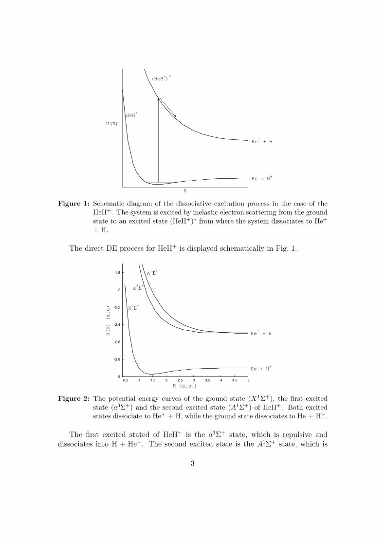
Figure 1: Schematic diagram of the dissociative excitation process in the case of theHeH+. The system is excited by inelastic electron scattering from the groundstate to an excited state (HeH+)∗ from where the system dissociates to He+
+ H.
The direct DE process for HeH+ is displayed schematically in Fig. 1.
-3
-2.8
-2.6
-2.4
-2.2
-2
-1.8
0.5 1 1.5 2 2.5 3 3.5 4 4.5 5
U(R) (a.u)
R (a.u.)
a3Σ+
X1Σ+
A1Σ+
He + H+
He+ + H
Figure 2: The potential energy curves of the ground state (X1Σ+), the first excitedstate (a3Σ+) and the second excited state (A1Σ+) of HeH+. Both excitedstates dissociate to He+ + H, while the ground state dissociates to He + H+.
The first excited stated of HeH+ is the a3Σ+ state, which is repulsive anddissociates into H + He+. The second excited state is the A1Σ+ state, which is
3
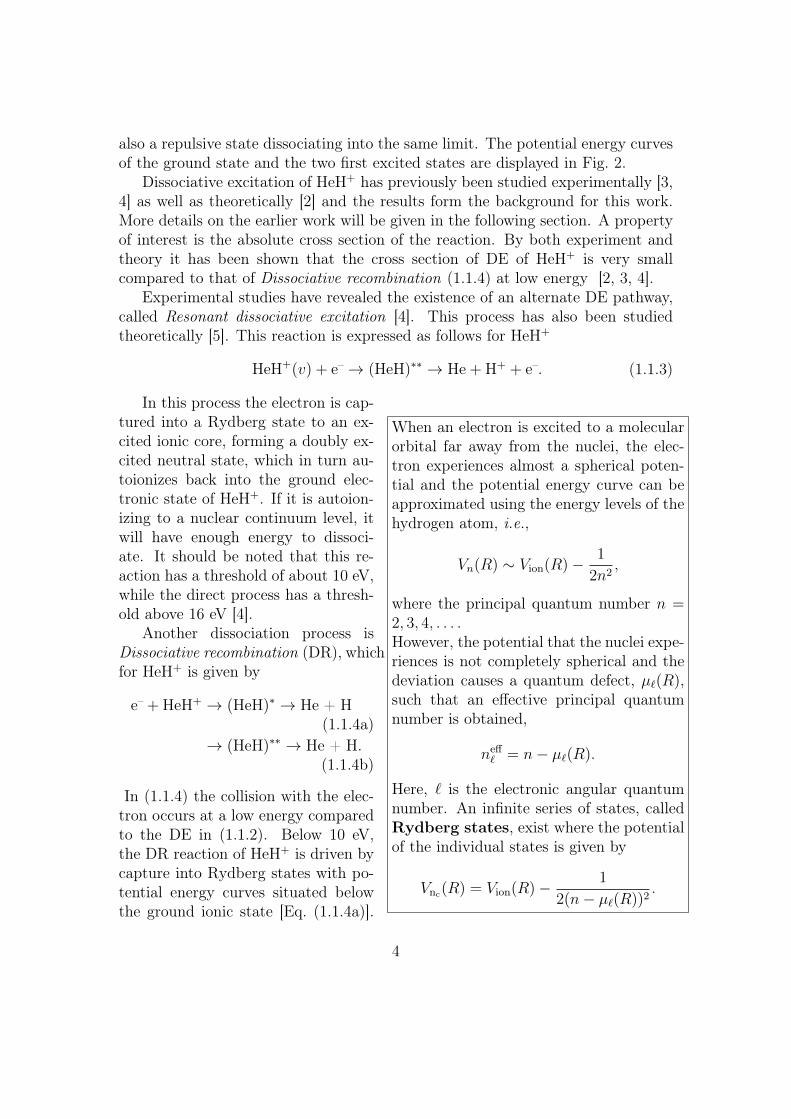
also a repulsive state dissociating into the same limit. The potential energy curvesof the ground state and the two first excited states are displayed in Fig. 2.
Dissociative excitation of HeH+ has previously been studied experimentally [3,4] as well as theoretically [2] and the results form the background for this work.More details on the earlier work will be given in the following section. A propertyof interest is the absolute cross section of the reaction. By both experiment andtheory it has been shown that the cross section of DE of HeH+ is very smallcompared to that of Dissociative recombination (1.1.4) at low energy [2, 3, 4].
Experimental studies have revealed the existence of an alternate DE pathway,called Resonant dissociative excitation [4]. This process has also been studiedtheoretically [5]. This reaction is expressed as follows for HeH+
HeH+(v) + e–→ (HeH)∗∗ → He + H+ + e–. (1.1.3)
When an electron is excited to a molecularorbital far away from the nuclei, the elec-tron experiences almost a spherical poten-tial and the potential energy curve can beapproximated using the energy levels of thehydrogen atom, i.e.,
Vn(R) ∼ Vion(R)− 1
2n2,
where the principal quantum number n =2, 3, 4, . . . .However, the potential that the nuclei expe-riences is not completely spherical and thedeviation causes a quantum defect, µ`(R),such that an effective principal quantumnumber is obtained,
neff` = n− µ`(R).
Here, ` is the electronic angular quantumnumber. An infinite series of states, calledRydberg states, exist where the potentialof the individual states is given by
Vnc(R) = Vion(R)− 1
2(n− µ`(R))2.
In this process the electron is cap-tured into a Rydberg state to an ex-cited ionic core, forming a doubly ex-cited neutral state, which in turn au-toionizes back into the ground elec-tronic state of HeH+. If it is autoion-izing to a nuclear continuum level, itwill have enough energy to dissoci-ate. It should be noted that this re-action has a threshold of about 10 eV,while the direct process has a thresh-old above 16 eV [4].
Another dissociation process isDissociative recombination (DR), whichfor HeH+ is given by
e– + HeH+ → (HeH)∗ → He + H(1.1.4a)
→ (HeH)∗∗ → He + H.(1.1.4b)
In (1.1.4) the collision with the elec-tron occurs at a low energy comparedto the DE in (1.1.2). Below 10 eV,the DR reaction of HeH+ is driven bycapture into Rydberg states with po-tential energy curves situated belowthe ground ionic state [Eq. (1.1.4a)].
4
Above 10 eV, the energy is high enough for capture into the doubly excited stateof HeH [Eq. (1.1.4b)] and the DR and the resonant DE are competing processes [4].
1.2 Earlier work on HeH+
As it was mentioned in subsection 1.1 there has not been as much work doneon DE as on other related processes, such as dissociative recombination. The mostcommon systems studied for DE is the hydrogen molecular ion. However, sinceHeH+ is a quite small system, it has also gained some previous attention. In thescope of this project both earlier experimental and theoretical works have beenstudied in order to gain insight in the DE process of HeH+ and have been used ascomparison for the result obtained using our method. Some of these studies havealready been referred to in subsection 1.1.
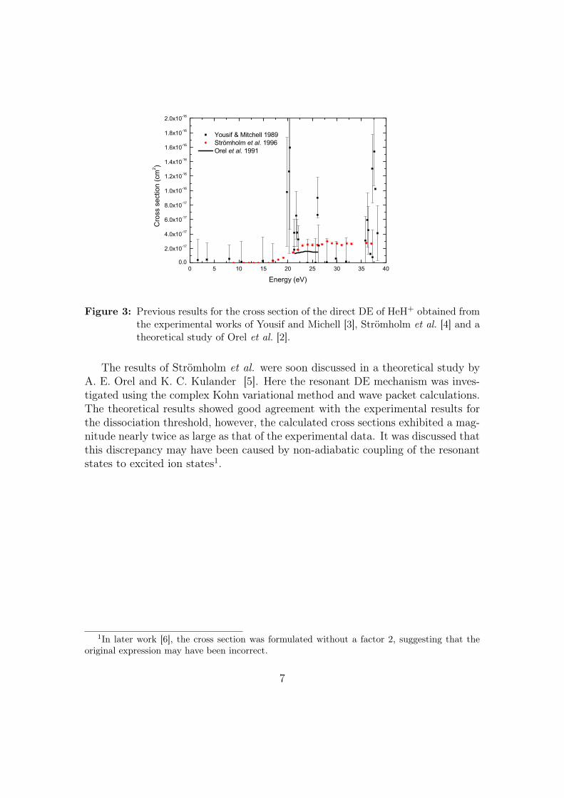
One of the earliest published experimental studies on DE of HeH+ is the workof F. B. Yousif and J. B. A. Mitchell from 1989 [3]. In this work the DR andDE processes of HeH+ were studied using a merged beam method. Yousif andMitchell reported the cross sections for DE in the 0 − 40 eV energy range. Theresults showed an excitation energy threshold at about 20 eV for the low extractionconditions, where the ions are believed to be mainly in the ground electronic state.Series of sharp and very narrow peaks in the cross section were detected in the20− 26 eV energy region. The narrowness of the peaks was suggested to originatefrom a process where the electron is trapped instantaneously into doubly excitedneutral resonant states.
The findings of Yousif and Mitchell prompted the theoretical study by A. E.Orel, T. N. Rescigno and B. H. Lengsfield III [2]. In this work the DE of HeH+
was studied in the 20 − 26 eV energy region using the complex Kohn variationalmethod [10, 14]. Excitation cross sections for the X1Σ+ → a3Σ
+ transition werecomputed in overall 2Σ+ and 2Π symmetries as well as the total cross sectionat the equilibrium separation (R0 = 0.77 Å). The calculation of the fixed-nucleicross section resulted in a series of sharp peaks on a quite flat background. Closerinspection showed that most of the peaks were Feshbach resonances associatedwith energetically closed Rydberg states in this energy region. One of the peaks,situated at 24 eV, did not belong to the above mentioned category but provedto be a core-excited shape resonance. Further, in the work of A. E. Orel, T. N.Rescigno and B. H. Lengsfield III [2], it was shown that an auto-ionization processfrom an doubly excited state, as suggested by Yousif and Mitchell, was not a viableexplanation of the narrowness of the peaks observed in the experiment.
The computations in 2Σ+ symmetry were also preformed at R = R0 ± 0.05 Åin order to investigate how the cross section responds to changes in the internu-clear distance. The results from these calculations showed that the widths of theresonance peaks and the value of the background cross section remained almost
5
unchanged. The positions of the peaks were shifted with the excitation energy ofthe X1Σ+ − A1Σ+ transition.
In this work a formula for calculating the averaged fixed-nuclei cross sectionwas also derived as follows
σ(E0) =
∫σ(E0, R)[χν0(R)]2dR. (1.2.1)
Here χν0 is the initial target vibrational wave function and σ(E0, R) is the "fixed-nuclei cross section". This formula, which will be presented and explained in moredetail in the Theory subsection 3.2, will be implemented in the scope of the presentwork.
When an averaged total excitation cross section was calculated, theR-dependenceof the excitation thresholds could therefore be included as a shift with respect toR0 and the sharp peaks observed in the fixed-nuclei cross section were smoothenedout.
A second experimental study of the DE of HeH+ was performed by C. Strömholmet al. [4]. In this work the DR and DE processes for HeH+ were studied and theabsolute cross sections were determined for energies below 40 eV. The experimentswere performed using CRYRING at the Manne Siegbahn Laboratory at Stock-holm University. Contrary to the results of the cross section obtained by Yousifand Mitchell, it was found here that the absolute cross section for the direct DEprocess was basically constant in the 21−37 eV energy region. Furthermore, it wasfound that there was an alternate DE pathway with an energy threshold alreadyat 10 eV. In the reaction the electron gets caught up in a neutral doubly excitedstate which auto-ionizes into He + H+. This reaction is the resonant dissociativeexcitation presented in subsection 1.1 and, as described above, it competes withthe DR process.
The results of the direct DE cross section for the HeH+ of the above mentionedstudies are displayed in Fig. 3.
6
0 5 10 15 20 25 30 35 400.0
2.0x10⁻¹⁷
4.0x10⁻¹⁷
6.0x10⁻¹⁷
8.0x10⁻¹⁷
1.0x10⁻¹⁶
1.2x10⁻¹⁶
1.4x10⁻¹⁶
1.6x10⁻¹⁶
1.8x10⁻¹⁶
2.0x10⁻¹⁶
Yousif & Mitchell 1989 Strömholm et al. 1996 Orel et al. 1991
Cro
ss s
ectio
n (c
m2 )
Energy (eV)
Figure 3: Previous results for the cross section of the direct DE of HeH+ obtained fromthe experimental works of Yousif and Michell [3], Strömholm et al. [4] and atheoretical study of Orel et al. [2].
The results of Strömholm et al. were soon discussed in a theoretical study byA. E. Orel and K. C. Kulander [5]. Here the resonant DE mechanism was inves-tigated using the complex Kohn variational method and wave packet calculations.The theoretical results showed good agreement with the experimental results forthe dissociation threshold, however, the calculated cross sections exhibited a mag-nitude nearly twice as large as that of the experimental data. It was discussed thatthis discrepancy may have been caused by non-adiabatic coupling of the resonantstates to excited ion states1.
1In later work [6], the cross section was formulated without a factor 2, suggesting that theoriginal expression may have been incorrect.
7
2 Theory
In this section the theoretical background relevant for this work will be related.The aim of this project is to develop a model using wave packets to describe thedirect dissociative excitation process of HeH+. Therefore the main focus of thissection will be to present the background of wave packet dynamics and the theorynecessary to understand the derivation of the cross section in section 3.
Even though it is far too complex to be related in full in the scope of thiswork some basic theory of electron scattering as well as a short introduction to thecomplex Kohn variational method (CKVM) [10] is included in this section. Neitherof these topics are comprised in the head part of this project, nevertheless, I feelthat a basic understanding is necessary to fully grasp the theoretical backgroundof this work.
This section starts with a brief introduction of the Born-Oppenheimer (BO)approximation [11] followed by a short presentation of quantum chemistry, wherespecifically the Multi-Reference Configuration Interaction (MRCI) method is dis-cussed. Note that atomic units (~ = e = me = a0 = 1) are used throughout. Formore details, conversion factors etc. see Appendix III - Conventions and notations.
2.1 The molecular Schrödinger equation and the Born-Oppenheimerapproximation
If the spin-orbit and relativistic interactions of the nuclei and electrons is ne-glected, the molecule can be described by means of the time-independent Schrödingerequation:
Hψ(R, r) = Etotψ(R, r). (2.1.1)
For this molecular system the Hamiltonian can be partitioned in the followingmanner
H = TN +He + VNN, (2.1.2)
where TN is the kinetic energy operator of the nuclei and VNN is the nuclear re-pulsion term. He, called the electronic Hamiltonian, consists of the kinetic energyoperator of the electrons as well as the electron-electron and electron-nuclei inter-actions. These terms can be expressed as follows.
TN = − 1
2µ∇2
R ≡ Tvib + Trot
He = −1
2
N∑i
∇2i −
2∑α
N∑i
Zαrαi
+N∑i
N∑j>i
1
rij
VNN =ZαZβR
.
(2.1.3)
8
Here the vibrational part of the nuclear kinetic energy operator is given by
Tvib = − 1
2µR2
∂
∂R
(R2 ∂
∂R
)(2.1.4)
and the rotational part by
Trot = − 1
2µR2
[1
sin θ
∂
∂θ
(sin θ
∂
∂θ
)+
1
sin2 θ
∂
∂ϕ2
]. (2.1.5)
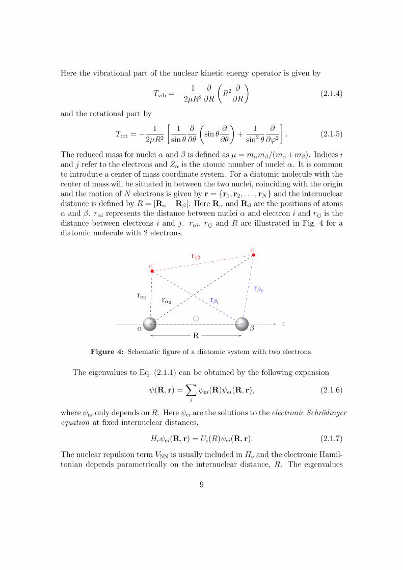
The reduced mass for nuclei α and β is defined as µ = mαmβ/(mα+mβ). Indices iand j refer to the electrons and Zα is the atomic number of nuclei α. It is commonto introduce a center of mass coordinate system. For a diatomic molecule with thecenter of mass will be situated in between the two nuclei, coinciding with the originand the motion of N electrons is given by r = r1, r2, . . . , rN and the internucleardistance is defined by R = |Rα−Rβ|. Here Rα and Rβ are the positions of atomsα and β. rαi represents the distance between nuclei α and electron i and rij is thedistance between electrons i and j. rαi, rij and R are illustrated in Fig. 4 for adiatomic molecule with 2 electrons.
z
r12
rα1
rβ2rβ1rα2
e–
e–
O
Rα β
Figure 4: Schematic figure of a diatomic system with two electrons.
The eigenvalues to Eq. (2.1.1) can be obtained by the following expansion
ψ(R, r) =∑i
ψni(R)ψei(R, r), (2.1.6)
where ψni only depends onR. Here ψei are the solutions to the electronic Schrödingerequation at fixed internuclear distances,
Heψei(R, r) = Ui(R)ψei(R, r). (2.1.7)
The nuclear repulsion term VNN is usually included in He and the electronic Hamil-tonian depends parametrically on the internuclear distance, R. The eigenvalues
9
to the electronic Schrödinger equation for the diatomic molecule form a potentialenergy curve Ui(R) of state i.
If Eqs. (2.1.2) and (2.1.6) are substituted into Eq. (2.1.1), the following expres-sion is obtained
[TN(R) +He(R, r)]∑i
ψni(R)ψei(R, r) = E∑i
ψni(R)ψei(R, r). (2.1.8)
Multiplying Eq. (2.1.8) with the electronic wave function ψ∗ej and integratingover electronic coordinates yields the following expression∑
i
〈ψej|TN +He|ψniψei〉 =∑i
〈ψej|E|ψniψei〉. (2.1.9)
Further, using the orthonormality, 〈ψei|ψej〉 = δij, and Eq. (2.1.7) we get∑i
〈ψej|TN|ψniψei〉+ Ujψnj = Eψnj, (2.1.10)
where j = 1, 2, 3, . . . . Eq. (2.1.10) is referred to as the nuclear Schrödinger equa-tion in the adiabatic representation. Evaluation of the first term of Eq. (2.1.10)will give rise to an infinite number of coupled differential equations for ψni. Theseequations cannot generally be solved analytically and approximations of the systemmust be made.
The Laplace operator of TN will affect both ψni and ψei as they both are Rdependent. Because of this the chain rule have to be applied on ψniψei and we getderivatives of both the nuclear and the electronic wave functions,
〈ψej|TN|ψniψei〉 = − 1
2µ〈ψej|∇2
R|ψniψei〉 = − 1
2µ〈ψej|∇R · (∇Rψniψei + ψni∇Rψei)〉
= − 1
2µ
[〈ψej|ψei〉∇2
Rψni + 2〈ψej|∇Rψei〉 · ∇Rψni + 〈ψej|∇2Rψei〉ψni
].
(2.1.11)Within the BO approximation we assume that TN operator has no effect on the
electronic wave function, meaning that non-adiabatic coupling elements 〈ψej|∇Rψei〉and 〈ψej|∇2
Rψei〉 can be neglected. This is a feasible assumption as the large dif-ference in particle weight makes the nuclei practically stationary compared to theelectrons. Using the BO approximation and the orthonormality of the electronicstates, Eq. (2.1.10) is simplified to
(TN + Uj(R))ψnj(R) = Eψnj(R). (2.1.12)
Thus, Eq. (2.1.12) provides a set of uncoupled equations for ψni, which is thenuclear wave function for the state i. The total wave function can now be obtainedaccording to Eq. (2.1.6)
ψ(R, r) = ψn(R)ψe(r, r). (2.1.13)
10
The Born-Oppenheimer approximation is usually valid for electronic groundstates that are well separated in energy from excited states. But for certain sys-tems the BO approximation is not always applicable. A system engaged with anionic bond will experience problems; at equilibrium distance the bond is essentiallyionic A+B−, however, at large separation the bond will instead be of covalent type.At a certain internuclear distance the potential energy curve of the covalent statebecomes very close to the energy of the ionic state. For a diatomic molecule the po-tential energy curves of the same electronic symmetry are not allowed to cross [12],instead an avoided crossing is formed where the electronic wave function changecharacter going from one side of the avoided crossing to the other. Close to theavoided crossing the non-adiabatic couplings are large and the BO approximationbreaks down.
2.2 Quantum chemistry and electronic structure calcula-tions
The electronic Schrödinger equation can only be solved analytically for one-electron systems, such as the H+
2 . For larger systems we have to rely on approx-imate methods. These methods use the variational principle to find approximatesolutions to the electronic Schrödinger equation, so called trial wave functions,ΦT, that are energy minimized with respect to some parameters in the trail wavefunction. The energy for normalized wave functions are given as
Ee = 〈ΦT|He|ΦT〉, (2.2.1)
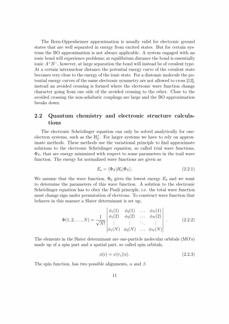
We assume that the wave function, Φ0 gives the lowest energy E0 and we wantto determine the parameters of this wave function. A solution to the electronicSchrödinger equation has to obey the Pauli principle, i.e. the total wave functionmust change sign under permutation of electrons. To construct wave function thatbehaves in this manner a Slater determinant is set up,
Φ(1, 2, . . . , N) =1√N !
∣∣∣∣∣∣∣∣∣φ1(1) φ2(1) . . . φN(1)φ1(2) φ2(2) . . . φN(2)...
... . . . ...φ1(N) φ2(N) . . . φN(N)
∣∣∣∣∣∣∣∣∣ . (2.2.2)
The elements in the Slater determinant are one-particle molecular orbitals (MO’s)made up of a spin part and a spatial part, so called spin orbitals,
φ(i) = ψ(ri)|s〉. (2.2.3)
The spin function, has two possible alignments, α and β.
11
There are many approaches to derive a trial wave function where the maindifference is how the electron correlation is included.
One method is the Configuration Interaction (CI) method. In standard CI thewave function is made up a linear combination of Slater determinants, also calledConfigurational State Functions (CSF’s), corresponding to different configurationswhere electrons have been excited, a so called configurational expansion.
ΨCI =∑i
ciΦi (2.2.4)
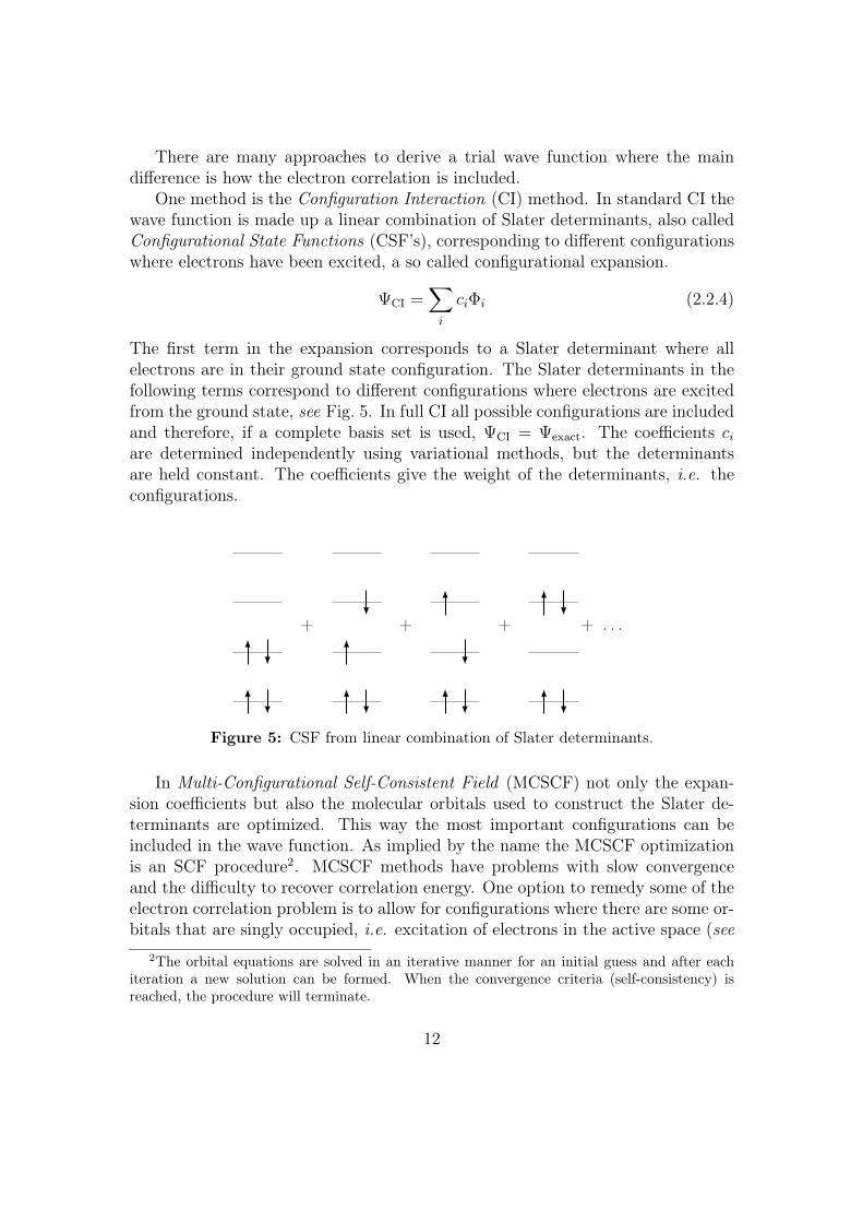
The first term in the expansion corresponds to a Slater determinant where allelectrons are in their ground state configuration. The Slater determinants in thefollowing terms correspond to different configurations where electrons are excitedfrom the ground state, see Fig. 5. In full CI all possible configurations are includedand therefore, if a complete basis set is used, ΨCI = Ψexact. The coefficients ciare determined independently using variational methods, but the determinantsare held constant. The coefficients give the weight of the determinants, i.e. theconfigurations.
+ + + + . . .
Figure 5: CSF from linear combination of Slater determinants.
In Multi-Configurational Self-Consistent Field (MCSCF) not only the expan-sion coefficients but also the molecular orbitals used to construct the Slater de-terminants are optimized. This way the most important configurations can beincluded in the wave function. As implied by the name the MCSCF optimizationis an SCF procedure2. MCSCF methods have problems with slow convergenceand the difficulty to recover correlation energy. One option to remedy some of theelectron correlation problem is to allow for configurations where there are some or-bitals that are singly occupied, i.e. excitation of electrons in the active space (see
2The orbital equations are solved in an iterative manner for an initial guess and after eachiteration a new solution can be formed. When the convergence criteria (self-consistency) isreached, the procedure will terminate.
12
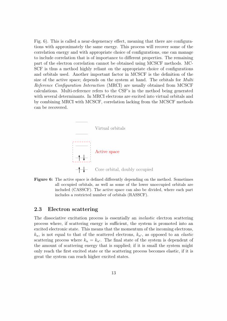
Fig. 6). This is called a near-degeneracy effect, meaning that there are configura-tions with approximately the same energy. This process will recover some of thecorrelation energy and with appropriate choice of configurations, one can manageto include correlation that is of importance to different properties. The remainingpart of the electron correlation cannot be obtained using MCSCF methods. MC-SCF is thus a method highly reliant on the appropriate choice of configurationsand orbitals used. Another important factor in MCSCF is the definition of thesize of the active space; depends on the system at hand. The orbitals for MultiReference Configuration Interaction (MRCI) are usually obtained from MCSCFcalculations. Multi-reference refers to the CSF’s in the method being generatedwith several determinants. In MRCI electrons are excited into virtual orbitals andby combining MRCI with MCSCF, correlation lacking from the MCSCF methodscan be recovered.
Active space
Virtual orbitals
Core orbital, doubly occupied
Figure 6: The active space is defined differently depending on the method. Sometimesall occupied orbitals, as well as some of the lower unoccupied orbitals areincluded (CASSCF). The active space can also be divided, where each partincludes a restricted number of orbitals (RASSCF).
2.3 Electron scattering
The dissociative excitation process is essentially an inelastic electron scatteringprocess where, if scattering energy is sufficient, the system is promoted into anexcited electronic state. This means that the momentum of the incoming electrons,kn, is not equal to that of the scattered electrons, kn′ , as opposed to an elasticscattering process where kn = kn′ . The final state of the system is dependent ofthe amount of scattering energy that is supplied; if it is small the system mightonly reach the first excited state or the scattering process becomes elastic, if it isgreat the system can reach higher excited states.
13
A scattering process where excitation is possible is said to be multi-channeland the different final states are called channels. A channel is called open if thesupplied scattering energy is sufficient to bring the system into the state. In thiswork we only consider the first and second excited electronic states of HeH+(seeFig. 2), in other words n′ = 1, 2 and we study the inelastic scattering 0 → 1 and0→ 2.
It is common to study the electron scattering process through means of thedifferential cross section and for the transition n→ n′ it is given by(
dσ
dΩ
)n→n′
=kn′
kn|fn′n(k′,k)|2. (2.3.1)
For the simplest case, elastic scattering, the differential cross section is simplygiven as the ratio of the scattered particles into the solid angle, dΩ, and thetotal number of incoming electrons per unit area. This ratio can be given by thesquare of the scattering amplitude, fn′n(k′,k). Another observable related to thedifferential cross section is the total cross section, which is obtained by integratingthe differential cross section over all solid angles,
σn→n′ =
∫ (dσ
dΩ
)n→n′
dΩ =
∫kn′
kn|fn′n(k′,k)|2dΩ. (2.3.2)
In this work the total inelastic scattering cross section will be calculated.
2.4 The adiabatic-nuclei approximation
In calculation of elastic electron scattering it is commonly assumed that thenuclei can be held fixed in space throughout the complete scattering process. Thisis a feasible approximation, as the velocity of the incoming electron is considerablyfaster than the rotational and vibrational motions of the nuclei [8]. It cannot befreely assumed that the fixed-nuclei approximation is applicable for all scatteringprocesses. However, electron scattering with a sufficiently high impact energy willmake the motions of the nuclei seem slow compared to the incident electron andthe nuclei position can be assumed fixed during the process. This theory is knownas the adiabatic-nuclei approximation and it was first derived by Chase 1956 [7]in the field of nuclear physics. The model of Chase has proven to be successfullyapplicable also to electron-molecule scattering processes [8].
The original adiabatic-nuclei approximation is derived not only for fixed nucleibut also for fixed target electrons. However, in electron-molecule scattering, theseelectrons must be allowed to move if we want to describe electronic excitation ofthe target. Based on the existing adiabatic-nuclei approximation, Shugard and
14
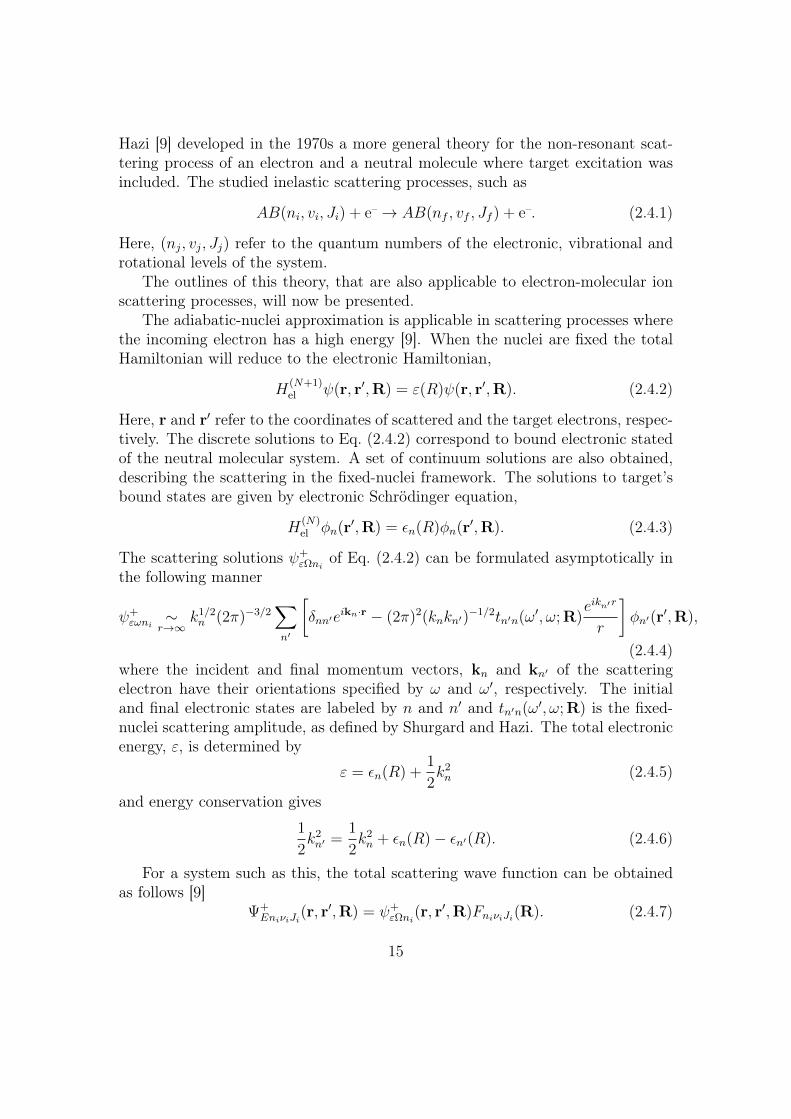
Hazi [9] developed in the 1970s a more general theory for the non-resonant scat-tering process of an electron and a neutral molecule where target excitation wasincluded. The studied inelastic scattering processes, such as
AB(ni, vi, Ji) + e–→ AB(nf , vf , Jf ) + e–. (2.4.1)
Here, (nj, vj, Jj) refer to the quantum numbers of the electronic, vibrational androtational levels of the system.
The outlines of this theory, that are also applicable to electron-molecular ionscattering processes, will now be presented.
The adiabatic-nuclei approximation is applicable in scattering processes wherethe incoming electron has a high energy [9]. When the nuclei are fixed the totalHamiltonian will reduce to the electronic Hamiltonian,
H(N+1)el ψ(r, r′,R) = ε(R)ψ(r, r′,R). (2.4.2)
Here, r and r′ refer to the coordinates of scattered and the target electrons, respec-tively. The discrete solutions to Eq. (2.4.2) correspond to bound electronic statedof the neutral molecular system. A set of continuum solutions are also obtained,describing the scattering in the fixed-nuclei framework. The solutions to target’sbound states are given by electronic Schrödinger equation,
H(N)el φn(r′,R) = εn(R)φn(r′,R). (2.4.3)
The scattering solutions ψ+εΩni
of Eq. (2.4.2) can be formulated asymptotically inthe following manner
ψ+εωni
∼r→∞
k1/2n (2π)−3/2
∑n′
[δnn′eikn·r − (2π)2(knkn′)−1/2tn′n(ω′, ω;R)
eikn′r
r
]φn′(r′,R),
(2.4.4)where the incident and final momentum vectors, kn and kn′ of the scatteringelectron have their orientations specified by ω and ω′, respectively. The initialand final electronic states are labeled by n and n′ and tn′n(ω′, ω;R) is the fixed-nuclei scattering amplitude, as defined by Shurgard and Hazi. The total electronicenergy, ε, is determined by
ε = εn(R) +1
2k2n (2.4.5)
and energy conservation gives
1
2k2n′ =
1
2k2n + εn(R)− εn′(R). (2.4.6)
For a system such as this, the total scattering wave function can be obtainedas follows [9]
Ψ+EniνiJi
(r, r′,R) = ψ+εΩni
(r, r′,R)FniνiJi(R). (2.4.7)
15
Here FnνJ are the nuclear functions of the Born-Oppenheimer product, defined asφn(r′,R)FnνJ(R), and satisfy[
− 1
2µ∇2
R + εn(R)− wnνJ]FnνJ(R) = 0, (2.4.8)
where wnνJ is the exact molecular energy in the adiabatic approximation.The use of the Born-Oppenheimer product is motivated by the assumption that
there is a lack of dynamical (non-adiabatic) coupling between the electron and thenuclei. This also implies that there is no such coupling in the target.
In Eq. (2.4.7) we have a wave function, consistent with the adiabatic-nucleiapproximation, where the electronic part is given by the fixed-nuclei function thatdescribes the electron-molecule scattering process in the fixed-nuclei framework.For this scattering process, the incoming electron will not contribute to the po-tential affecting the nuclei. The reason for this is the limited time the electronis present in the vicinity of the nuclei. This implies that FniνiJi(R) is the ro-vibrational wave function of the target’s initial state [9].
Knowing the expression for the total wave function enables us to determine thetotal scattering amplitude [9]
TnfνfJf ,niνiJi(Ω′Ω) =
∫dRF ∗nfνfJf (R)tnfni(Ω
′,Ω;R)FniνiJi(R)
(kfknf
)ei(knf−kf )r.
(2.4.9)Here knf and kni are the fixed-nuclei momenta of the final and initial states, re-spectively and they are related by Eq. (2.4.6), where kni ≡ ki [9]. The direction ofthe incident and final momentum vectors, ki and kf , is specified by Ω and Ω′.
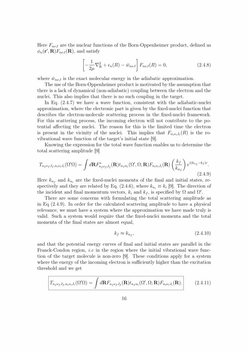
There are some concerns with formulating the total scattering amplitude asin Eq (2.4.9). In order for the calculated scattering amplitude to have a physicalrelevance, we must have a system where the approximation we have made truly isvalid. Such a system would require that the fixed-nuclei momenta and the totalmomenta of the final states are almost equal,
kf ≈ knf , (2.4.10)
and that the potential energy curves of final and initial states are parallel in theFranck-Condon region, i.e in the region where the initial vibrational wave func-tion of the target molecule is non-zero [9]. These conditions apply for a systemwhere the energy of the incoming electron is sufficiently higher than the excitationthreshold and we get
TnfνfJf ,niνiJi(Ω′Ω) =
∫dRFnfνfJf (R)tnfni(Ω
′,Ω;R)FniνiJi(R). (2.4.11)
16
Thus, for systems where the impact energy is higher than the excitation threshold,the T -matrix elements can be obtained by averaging the fixed-nuclei amplitudeover the initial and final ro-vibrational wave functions [9].
Up to this point, the electron scattering process has been considered on theenergy shell. However, for reasons soon to be apparent, it is also common toevaluate the scattering amplitude off the energy shell.
When the electron scattering is calculated off the energy shell, we have thatkf 6= knf and ε′ 6= ε, i.e. the initial and final energy of the scattered electrons arenot the same [9].
Due to the restrictions mentioned earlier, the on-shell T -matrix fails to describethe electron scattering process near the excitation threshold. Therefore, an im-proved formulation of the scattering amplitude evaluated off the energy shell wasalso suggested by Shugard and Hazi,
TnfνfJf ,niνiJi(Ω′Ω) =
∫dRFnfνfJf (R)tnfni(ε
′Ω′, εΩ;R)FniνiJi(R). (2.4.12)
Here, the T-matrix has been expressed off-shell with the energy ε defined as inEq. (2.4.5) and ε′ given as
ε′ = εnf (R) +1
2k2f . (2.4.13)
Here tnfni(ε′Ω′, εΩ;R) is the fixed-nuclei scattering amplitude expressed off theenergy shell. In the case where the impact energy is greater than the excitationthreshold, the off-shell quantities are the same as their corresponding on-shellforms.
The off-shell formulation should give better results for systems where the scat-tering process occurs close to the excitation threshold as the off-shell kf does nothave to be restricted by Eq. (2.4.10). However, the off-shell tnfni must be calcu-lated separately for each ro-vibrational state, as the quantum numbers (nfνfJf )are needed to determine the magnitude of kf .
2.5 Complex Kohn variational method
The fixed-nuclei electron scattering calculations were performed using an alge-braic variational technique called the Complex Kohn variational method (CKVM) [10].A trial wave function is created and inserted into a functional which, in turn, isminimized with respect to certain parameters. The basic approach of the CKVMfor scattering of an electron-ion system with a spherically symmetric, short-rangepotential V (r) will now be illustrated [10]. The partial wave radial Schrödingerequation can be given in the following manner
LΦ` = 0, (2.5.1)
17
where L is given by
L =
[−1
2
d2
dr2+`(`+ 1)
2r2+Z
r+ V (r)− k2
2
]. (2.5.2)
A functional, commonly called the Kohn functional I, is defined as follows
I[Φ`] =
∫ ∞0
Φ`(r)LΦ`(r)dr. (2.5.3)
The functional I[Φ`] = 0 if Φ` represents the exact solution. If instead a trialfunction, Φt
` 6= Φ`, is inserted in Eq. (2.5.3), the functional will differ from zero. Itis assumed that the following boundary conditions will apply to Φ`:
Φ`(0) = 0
Φ`(r →∞) ∼ F`(kr) + λG`(kr).(2.5.4)
The Coulomb functions F` and G` are linearly independent solutions of Eq. (2.5.1)for the case where V (r) = 0 and λ is a linear coefficient. In order to study howthe functional, I, behaves when a trial function is inserted in Eq. (2.5.1), we firsthave to define the deviance of Φt
` from the exact solution Φ`,
δΦ`(r) ≡ Φt`(r)− Φ`(r). (2.5.5)
δΦ`(r) is called the residual and it applied to the following boundary conditions
δΦ`(0) = 0
δΦ`(r →∞) ∼ λG`(kr).(2.5.6)
If Eq. (2.5.5) is substituted into the Kohn functional the following result is obtainedafter some simplification [10]
δI = −k2Wδλ+
∫ ∞0
δΦ`LδΦ`dr. (2.5.7)
The Wronskian, W , is given by
W = F`(r)d
drG`(r)−G`(r)
d
drF`(r) (2.5.8)
and δλ = λ− λt, where λt is a variational parameter and λ is the exact value. Fora more detailed derivation of Eq. (2.5.7) refer to e.g [10]. Eq. (2.5.7) is called theKato identity and it approximates λ with a stationary principle in the followingmanner:
λs = λt +2
kW
∫ ∞0
Φt`LΦt
`dr. (2.5.9)
18
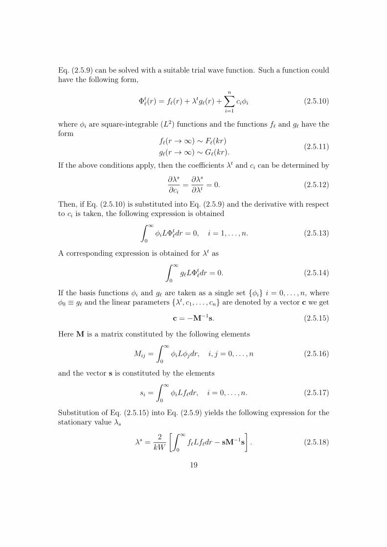
Eq. (2.5.9) can be solved with a suitable trial wave function. Such a function couldhave the following form,
Φt`(r) = f`(r) + λtg`(r) +
n∑i=1
ciφi (2.5.10)
where φi are square-integrable (L2) functions and the functions f` and g` have theform
f`(r →∞) ∼ F`(kr)
g`(r →∞) ∼ G`(kr).(2.5.11)
If the above conditions apply, then the coefficients λt and ci can be determined by
∂λs
∂ci=∂λs
∂λt= 0. (2.5.12)
Then, if Eq. (2.5.10) is substituted into Eq. (2.5.9) and the derivative with respectto ci is taken, the following expression is obtained∫ ∞
0
φiLΦt`dr = 0, i = 1, . . . , n. (2.5.13)
A corresponding expression is obtained for λt as∫ ∞0
g`LΦt`dr = 0. (2.5.14)
If the basis functions φi and g` are taken as a single set φi i = 0, . . . , n, whereφ0 ≡ g` and the linear parameters λt, c1, . . . , cn are denoted by a vector c we get
c = −M−1s. (2.5.15)
Here M is a matrix constituted by the following elements
Mij =
∫ ∞0
φiLφjdr, i, j = 0, . . . , n (2.5.16)
and the vector s is constituted by the elements
si =
∫ ∞0
φiLf`dr, i = 0, . . . , n. (2.5.17)
Substitution of Eq. (2.5.15) into Eq. (2.5.9) yields the following expression for thestationary value λs
λs =2
kW
[∫ ∞0
f`Lf`dr − sM−1s
]. (2.5.18)
19
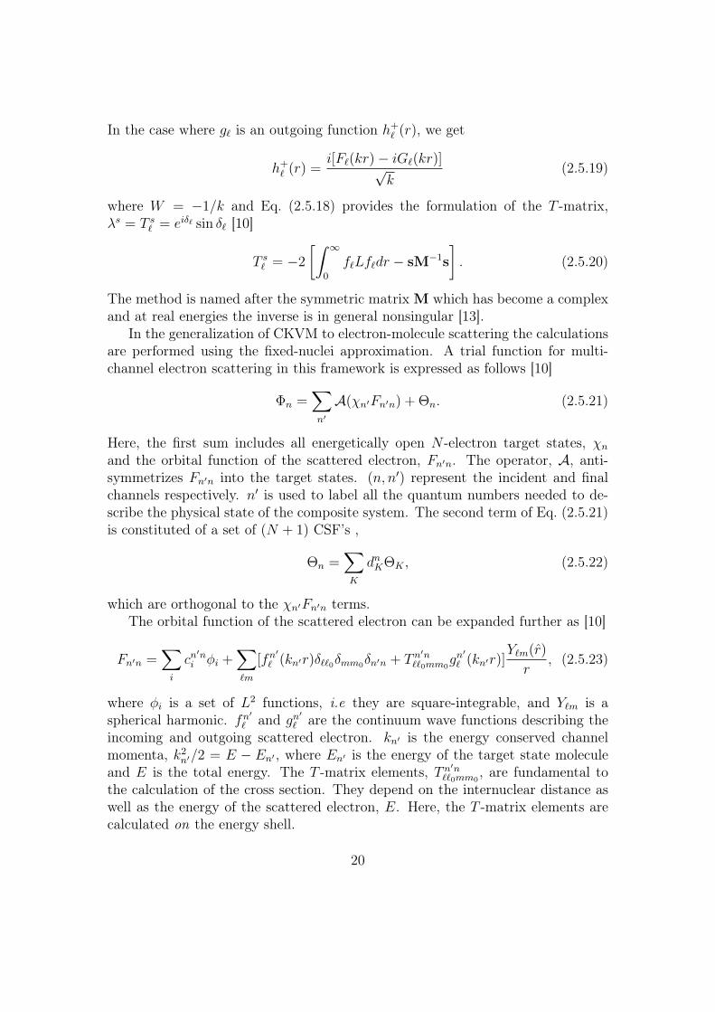
In the case where g` is an outgoing function h+` (r), we get
h+` (r) =
i[F`(kr)− iG`(kr)]√k
(2.5.19)
where W = −1/k and Eq. (2.5.18) provides the formulation of the T -matrix,λs = T s` = eiδ` sin δ` [10]
T s` = −2
[∫ ∞0
f`Lf`dr − sM−1s
]. (2.5.20)
The method is named after the symmetric matrix M which has become a complexand at real energies the inverse is in general nonsingular [13].
In the generalization of CKVM to electron-molecule scattering the calculationsare performed using the fixed-nuclei approximation. A trial function for multi-channel electron scattering in this framework is expressed as follows [10]
Φn =∑n′
A(χn′Fn′n) + Θn. (2.5.21)
Here, the first sum includes all energetically open N -electron target states, χnand the orbital function of the scattered electron, Fn′n. The operator, A, anti-symmetrizes Fn′n into the target states. (n, n′) represent the incident and finalchannels respectively. n′ is used to label all the quantum numbers needed to de-scribe the physical state of the composite system. The second term of Eq. (2.5.21)is constituted of a set of (N + 1) CSF’s ,
Θn =∑K
dnKΘK , (2.5.22)
which are orthogonal to the χn′Fn′n terms.The orbital function of the scattered electron can be expanded further as [10]
Fn′n =∑i
cn′ni φi +
∑`m
[fn′
` (kn′r)δ``0δmm0δn′n + T n′n
``0mm0gn
′
` (kn′r)]Y`m(r)
r, (2.5.23)
where φi is a set of L2 functions, i.e they are square-integrable, and Y`m is aspherical harmonic. fn′
` and gn′
` are the continuum wave functions describing theincoming and outgoing scattered electron. kn′ is the energy conserved channelmomenta, k2
n′/2 = E − En′ , where En′ is the energy of the target state moleculeand E is the total energy. The T -matrix elements, T n′n
``0mm0, are fundamental to
the calculation of the cross section. They depend on the internuclear distance aswell as the energy of the scattered electron, E. Here, the T -matrix elements arecalculated on the energy shell.
20
2.6 Wave packet methods
It was seen in the Introduction that in DE the inelastic electron scattering willtransfer the molecular ion from the ground state to an excited electronic state. Theexcited system will have a specific total energy depending on the electron scatteringenergy and the initial state of the target ion and the process is usually describedtime-independently. However, in order to easily incorporate quantum effects andfollow the process in time, the full time-dependent Schrödinger equation has tobe solved and the wave packets are the solutions. However, before introducingthe definition of a wave packet it makes sense to first discuss why it needs to beconstructed.
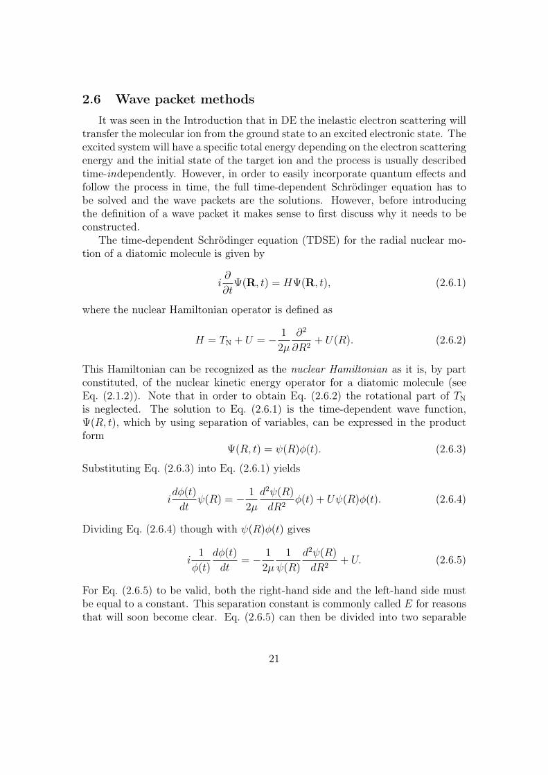
The time-dependent Schrödinger equation (TDSE) for the radial nuclear mo-tion of a diatomic molecule is given by
i∂
∂tΨ(R, t) = HΨ(R, t), (2.6.1)
where the nuclear Hamiltonian operator is defined as
H = TN + U = − 1
2µ
∂2
∂R2+ U(R). (2.6.2)
This Hamiltonian can be recognized as the nuclear Hamiltonian as it is, by partconstituted, of the nuclear kinetic energy operator for a diatomic molecule (seeEq. (2.1.2)). Note that in order to obtain Eq. (2.6.2) the rotational part of TNis neglected. The solution to Eq. (2.6.1) is the time-dependent wave function,Ψ(R, t), which by using separation of variables, can be expressed in the productform
Ψ(R, t) = ψ(R)φ(t). (2.6.3)
Substituting Eq. (2.6.3) into Eq. (2.6.1) yields
idφ(t)
dtψ(R) = − 1
2µ
d2ψ(R)
dR2φ(t) + Uψ(R)φ(t). (2.6.4)
Dividing Eq. (2.6.4) though with ψ(R)φ(t) gives
i1
φ(t)
dφ(t)
dt= − 1
2µ
1
ψ(R)
d2ψ(R)
dR2+ U. (2.6.5)
For Eq. (2.6.5) to be valid, both the right-hand side and the left-hand side mustbe equal to a constant. This separation constant is commonly called E for reasonsthat will soon become clear. Eq. (2.6.5) can then be divided into two separable
21
equations in the following manner
idφ(t)
dt= Eφ(t)
− 1
2µ
d2ψE(R)
dR2+ UψE(R) = EψE(R).
(2.6.6)
The second equation of (2.6.6) we recognize as the time-independent Schrödingerequation for the nuclear motion.
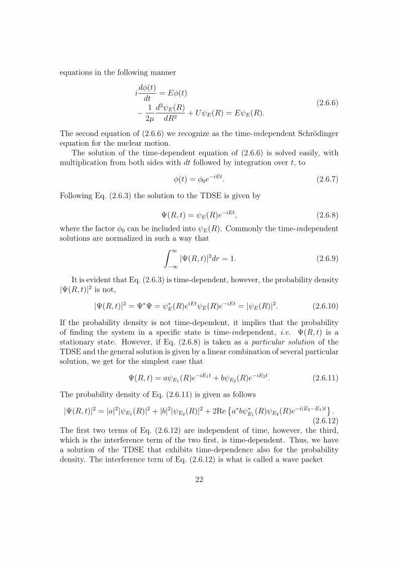
The solution of the time-dependent equation of (2.6.6) is solved easily, withmultiplication from both sides with dt followed by integration over t, to
φ(t) = φ0e−iEt. (2.6.7)
Following Eq. (2.6.3) the solution to the TDSE is given by
Ψ(R, t) = ψE(R)e−iEt, (2.6.8)
where the factor φ0 can be included into ψE(R). Commonly the time-independentsolutions are normalized in such a way that∫ ∞
−∞|Ψ(R, t)|2dr = 1. (2.6.9)
It is evident that Eq. (2.6.3) is time-dependent, however, the probability density|Ψ(R, t)|2 is not,
|Ψ(R, t)|2 = Ψ∗Ψ = ψ∗E(R)eiEtψE(R)e−iEt = |ψE(R)|2. (2.6.10)
If the probability density is not time-dependent, it implies that the probabilityof finding the system in a specific state is time-independent, i.e. Ψ(R, t) is astationary state. However, if Eq. (2.6.8) is taken as a particular solution of theTDSE and the general solution is given by a linear combination of several particularsolution, we get for the simplest case that
Ψ(R, t) = aψE1(R)e−iE1t + bψE2(R)e−iE2t. (2.6.11)
The probability density of Eq. (2.6.11) is given as follows
|Ψ(R, t)|2 = |a|2|ψE1(R)|2 + |b|2|ψE2(R)|2 + 2Rea∗bψ∗E1
(R)ψE2(R)e−i(E2−E1)t.
(2.6.12)The first two terms of Eq. (2.6.12) are independent of time, however, the third,which is the interference term of the two first, is time-dependent. Thus, we havea solution of the TDSE that exhibits time-dependence also for the probabilitydensity. The interference term of Eq. (2.6.12) is what is called a wave packet
22
- a wave packet is the superposition of states of different energies, whichis required in order to get a solution that has time-dependence in theprobability density and other observable quantities [17].
The general solution of the TDSE is given as
Ψ(R, t) =∞∑n=1
anψn(R)e−iEnt. (2.6.13)
Eq. (2.6.13) applies when the system has bound potential, resulting in solutionsthat only exist at certain discrete energies. The energy range in which physicallyinteresting solutions can be found is called the spectrum; i.e. Eq. (2.6.13) gives thesolution in a discrete spectrum. If the system constitutes an unbound potential,the interesting solutions are found in a continuous energy interval, rather than atdiscrete energies. The wave function for systems like this is given by
Ψ(R, t) =
∫ ∞0
a(E)ψE(R)e−iEtdE. (2.6.14)
Thus, the solution of the TDSE in a continuous spectrum is given by Eq. (2.6.14).When we know why it is needed, it makes sense to derive an actual wave packet.
The simplest TDSE is the given for the free particle and the Hamiltonian for thissystem is defined as
H = − 1
2µ
∂2R
∂R2, (2.6.15)
where the potential function is independent of the position and is taken as U(R) =0. The time-independent solution is given as
ψE(R) = e±ikR, (2.6.16)
with the energy eigenvalues E forming a continuous spectrum
E =k2
2µ=p2
2µ. (2.6.17)
By Eq. (2.6.8) a time-dependent particular solution to the TDSE is obtained as
Ψ(R, t) = eikRe−iEt = ei(kR−k2
2µt), (2.6.18)
where k goes from −∞ to ∞. Substituting Eq. (2.6.19) into Eq. (2.6.14) we getthe solution in the continuous spectrum
Ψ(R, t) =
∫ ∞−∞
a(k)ei(kR−k2
2µt)dk. (2.6.19)
23
The initial condition of the wave packet, i.e. for t = 0, can easily be determinedfrom Eq. (2.6.19),
Ψ(R, 0) =
∫ ∞−∞
a(k)eikRdk. (2.6.20)
To determine the function a(k) it is convenient to use Fourier transformation, Ap-pendix I. Eq. (2.6.20) can rewritten as a Fourier transformation by multiplicationof both sides by e−ik
′R and integrating over R. Using the Dirac delta function(Appendix I) we get
a(k) =1
2π
∫ ∞−∞
Ψ(R, 0)e−ikRdR. (2.6.21)
Thus, Ψ(R, 0) and a(k) are a Fourier pair. The same applies for the generalsolution
Ψ(R, t) =
∫ ∞−∞
a(k, t)eikRdk (2.6.22)
when the function a(k, t) is defined as follows
a(k, t) = a(k)e−ik2
2µt. (2.6.23)
Similarly for a(k, t) we get
a(k, t) =1
2π
∫ ∞−∞
Ψ(R, t)e−ikRdR, (2.6.24)
making Ψ(R, t) and a(k, t) another Fourier pair.
24
3 Derivation of cross section
With the theoretical background gained in section 2, we can now continueon to the cross section. In this section a time-dependent expression of the crosssection of DE is derived from the more common time-independent form. With thetime-dependent method, wave packet propagation is used to compute the crosssection of dissociative excitation. A similar approach has been used to obtain thecross section of photodissociation.
This section begins with a short description of the work performed on pho-todissociation.
3.1 Cross section of photodissociation
Photodissociation is the process wherein a molecule is excited from the groundelectronic state to an excited electronic state by absorption of a photon. Themolecule then dissociates, either directly, or in a delayed fashion, depending onthe nature of the potential of the excited state. Molecular processes like photodis-sociation can be studied using wave packets, a method that was seen early in thework of E. Heller in the 1970s [15, 16].
A property called the total absorption cross section σ, which provides a measureof the amount of light, with energy ω (atomic units), that can be absorbed by thesystem, can be used to study the photodissociation process. The cross sectioncan be formulated time-independently or time-dependently. The derivation froma time-independent description to a time-dependent will now be given.
The total cross section of photodissociation can be defined in the followingmanner [15],
σ(ω) ∝ ω|〈ψ−(E)|µtd|χi〉|2 ≡ ωΣ(ω), (3.1.1)
Here ψ−(E) is the energy-normalized scattering eigenstate with the energy E =Ei + ω. Furthermore, |χi〉 is the initial vibrational state and µtd is the transi-tion dipole matrix element connecting the initial and final electronic states3. Analternative expression of Σ can also be obtained by
Σ(ω) = 〈φ|ψ−(E)〉〈ψ−(E)|φ〉 (3.1.2)
where |φ〉 ≡ µtd|χi〉. The outgoing scattering states form a complete basis, i.e.
1 =
∫|ψ−(E ′)〉〈ψ−(E ′)|dE ′. (3.1.3)
3The elements of the transition dipole matrix are give by µtd = 〈φf |µ|φi〉.
25
Thus ψ−(E ′) can be rewritten using the Dirac delta function in the followingmanner,
δ(E −H) = δ(E −H) · 1 = |ψ−(E)〉〈ψ−(E)|, (3.1.4)
where H is the full Hamiltonian of the excited state. Substituting Eq. (3.1.4) intoEq. (3.1.2) yields
Σ(ω) = 〈φ|δ(E −H)|φ〉 = Trδ(E −H)|φ〉〈φ|. (3.1.5)
Remembering that the Fourier transform of the Dirac-delta function is given by(see Appendix I subsection A.2)
δ(E −H) =1
2π
∫ ∞−∞
eit(E−H)dt, (3.1.6)
Σ(ω) can be expressed in the following manner
Σ(ω) =1
2π
∫ ∞−∞〈φ|eit(E−H)|φ〉dt =
1
2π
∫ ∞−∞
eiEt〈φ|e−iHt|φ〉dt
=1
2π
∫ ∞−∞
eiEt〈φ(0)|φ(t)〉dt,(3.1.7)
where φ(t) is defined as follows
φ(t) = e−iHt|φ〉. (3.1.8)
From Eq. (3.1.7) it is evident that
the total photodissociation cross section is proportional to the Fouriertransform of the overlap of the initial wave function φ(0) and the wavefunction when it has been propagated on the energy surface of the excitedstate [15].
An alternative formulation is that the Fourier transform of the autocorrelationof a wave packet propagated on the potential energy surface is the total crosssection.
With the total cross section defined according to Eq. (3.1.7), it can further beshown that |A(t)| is even around t = 0, where A(t) ≡ 〈φ(0)|φ(τ)〉 is defined to bethe correlation function [16]. Using Eq. (3.1.8) it is straight forward to show that
A∗(t) = A(−t). (3.1.9)
From Eq. (3.1.9) it follows that Σ(ω) is real [16].More details of the autocorrelation function can be found in Appendix I sub-
section A.3.
26
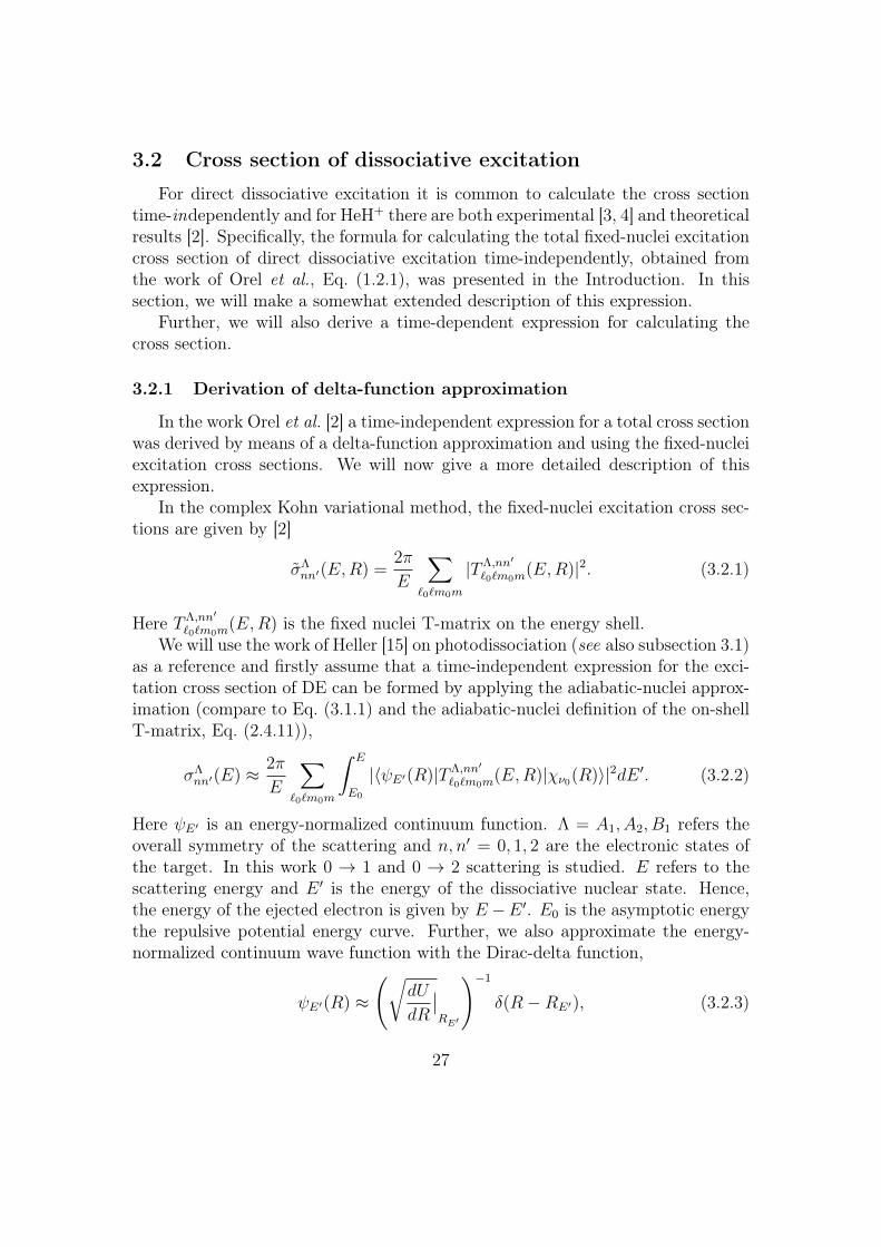
3.2 Cross section of dissociative excitation
For direct dissociative excitation it is common to calculate the cross sectiontime-independently and for HeH+ there are both experimental [3, 4] and theoreticalresults [2]. Specifically, the formula for calculating the total fixed-nuclei excitationcross section of direct dissociative excitation time-independently, obtained fromthe work of Orel et al., Eq. (1.2.1), was presented in the Introduction. In thissection, we will make a somewhat extended description of this expression.
Further, we will also derive a time-dependent expression for calculating thecross section.
3.2.1 Derivation of delta-function approximation
In the work Orel et al. [2] a time-independent expression for a total cross sectionwas derived by means of a delta-function approximation and using the fixed-nucleiexcitation cross sections. We will now give a more detailed description of thisexpression.
In the complex Kohn variational method, the fixed-nuclei excitation cross sec-tions are given by [2]
σΛnn′(E,R) =
2π
E
∑`0`m0m
|TΛ,nn′
`0`m0m(E,R)|2. (3.2.1)
Here TΛ,nn′
`0`m0m(E,R) is the fixed nuclei T-matrix on the energy shell.
We will use the work of Heller [15] on photodissociation (see also subsection 3.1)as a reference and firstly assume that a time-independent expression for the exci-tation cross section of DE can be formed by applying the adiabatic-nuclei approx-imation (compare to Eq. (3.1.1) and the adiabatic-nuclei definition of the on-shellT-matrix, Eq. (2.4.11)),
σΛnn′(E) ≈ 2π
E
∑`0`m0m
∫ E
E0
|〈ψE′(R)|TΛ,nn′
`0`m0m(E,R)|χν0(R)〉|2dE ′. (3.2.2)
Here ψE′ is an energy-normalized continuum function. Λ = A1, A2, B1 refers theoverall symmetry of the scattering and n, n′ = 0, 1, 2 are the electronic states ofthe target. In this work 0 → 1 and 0 → 2 scattering is studied. E refers to thescattering energy and E ′ is the energy of the dissociative nuclear state. Hence,the energy of the ejected electron is given by E −E ′. E0 is the asymptotic energythe repulsive potential energy curve. Further, we also approximate the energy-normalized continuum wave function with the Dirac-delta function,
ψE′(R) ≈
(√dU
dR
∣∣RE′
)−1
δ(R−RE′), (3.2.3)
27
where U(R) is the potential energy curve excited ionic state and RE′ is the classicalturning point at energy E ′. Inserting Eq. (3.2.3) into Eq. (3.2.2) yields
σΛnn′(E) ≈ 2π
E
∫ E
E0
(dU
dR
∣∣RE′
)−1 ∑`0`m0m
|TΛ,nn′
`0`m0m(E,RE′)|2[χν0(RE′)]2dE ′. (3.2.4)
Hence, we can write Eq. (3.2.4) as
σΛnn′(E) =
∫ E
E0
(dU
dR
∣∣RE′
)−1
σΛnn′(E,RE′)[χν0(RE′)]2dE ′. (3.2.5)
Making the following change of variables,
U(RE′) = E ′
dE ′ =dU
dRE′dRE′ ,
(3.2.6)
yields the following expression
σΛnn′(E) =
∫ ∞RE
σΛnn′(E,R)[χν0(R)]2dR. (3.2.7)
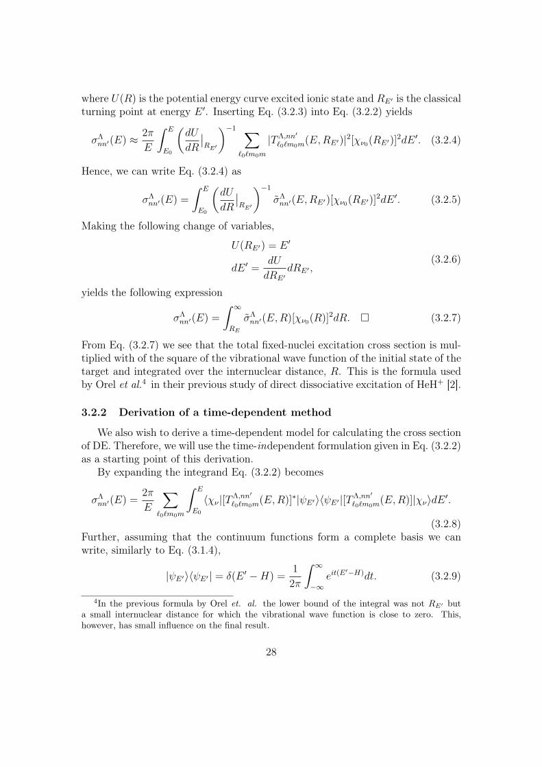
From Eq. (3.2.7) we see that the total fixed-nuclei excitation cross section is mul-tiplied with of the square of the vibrational wave function of the initial state of thetarget and integrated over the internuclear distance, R. This is the formula usedby Orel et al.4 in their previous study of direct dissociative excitation of HeH+ [2].
3.2.2 Derivation of a time-dependent method
We also wish to derive a time-dependent model for calculating the cross sectionof DE. Therefore, we will use the time-independent formulation given in Eq. (3.2.2)as a starting point of this derivation.
By expanding the integrand Eq. (3.2.2) becomes
σΛnn′(E) =
2π
E
∑`0`m0m
∫ E
E0
〈χν |[TΛ,nn′
`0`m0m(E,R)]∗|ψE′〉〈ψE′ |[TΛ,nn′
`0`m0m(E,R)]|χν〉dE ′.
(3.2.8)Further, assuming that the continuum functions form a complete basis we canwrite, similarly to Eq. (3.1.4),
|ψE′〉〈ψE′ | = δ(E ′ −H) =1
2π
∫ ∞−∞
eit(E′−H)dt. (3.2.9)
4In the previous formula by Orel et. al. the lower bound of the integral was not RE′ buta small internuclear distance for which the vibrational wave function is close to zero. This,however, has small influence on the final result.
28
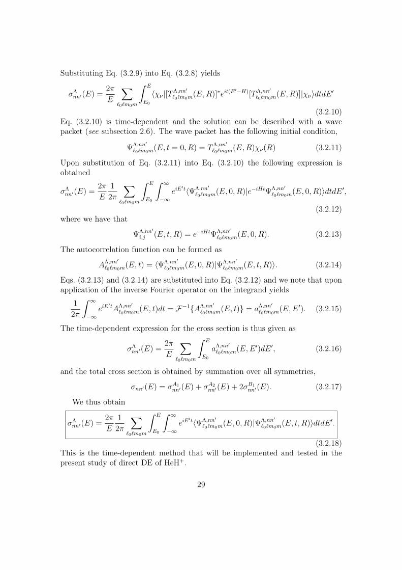
Substituting Eq. (3.2.9) into Eq. (3.2.8) yields
σΛnn′(E) =
2π
E
∑`0`m0m
∫ E
E0
〈χν |[TΛ,nn′
`0`m0m(E,R)]∗eit(E
′−H)[TΛ,nn′
`0`m0m(E,R)]|χν〉dtdE ′
(3.2.10)Eq. (3.2.10) is time-dependent and the solution can be described with a wavepacket (see subsection 2.6). The wave packet has the following initial condition,
ΨΛ,nn′
`0`m0m(E, t = 0, R) = TΛ,nn′
`0`m0m(E,R)χν(R) (3.2.11)
Upon substitution of Eq. (3.2.11) into Eq. (3.2.10) the following expression isobtained
σΛnn′(E) =
2π
E
1
2π
∑`0`m0m
∫ E
E0
∫ ∞−∞
eiE′t〈ΨΛ,nn′
`0`m0m(E, 0, R)|e−iHtΨΛ,nn′
`0`m0m(E, 0, R)〉dtdE ′,
(3.2.12)where we have that
ΨΛ,nn′
i,j (E, t, R) = e−iHtΨΛ,nn′
`0`m0m(E, 0, R). (3.2.13)
The autocorrelation function can be formed as
AΛ,nn′
`0`m0m(E, t) = 〈ΨΛ,nn′
`0`m0m(E, 0, R)|ΨΛ,nn′
`0`m0m(E, t, R)〉. (3.2.14)
Eqs. (3.2.13) and (3.2.14) are substituted into Eq. (3.2.12) and we note that uponapplication of the inverse Fourier operator on the integrand yields
1
2π
∫ ∞−∞
eiE′tAΛ,nn′
`0`m0m(E, t)dt = F−1AΛ,nn′
`0`m0m(E, t) = aΛ,nn′
`0`m0m(E,E ′). (3.2.15)
The time-dependent expression for the cross section is thus given as
σΛnn′(E) =
2π
E
∑`0`m0m
∫ E
E0
aΛ,nn′
`0`m0m(E,E ′)dE ′, (3.2.16)
and the total cross section is obtained by summation over all symmetries,
σnn′(E) = σA1
nn′(E) + σA2
nn′(E) + 2σB1
nn′(E). (3.2.17)
We thus obtain
σΛnn′(E) =
2π
E
1
2π
∑`0`m0m
∫ E
E0
∫ ∞−∞
eiE′t〈ΨΛ,nn′
`0`m0m(E, 0, R)|ΨΛ,nn′
`0`m0m(E, t, R)〉dtdE ′.
(3.2.18)This is the time-dependent method that will be implemented and tested in thepresent study of direct DE of HeH+.
29
4 Computational Details
In this section computational details on the electronic structure calculationsand electron scattering calculations that form the input for the calculation of thecross section will be given. The choice of symmetry in which these calculationsare preformed will also be briefly explained.
Further, the implementation of the time-independent and time-dependent ex-pressions for calculating the cross section of DE, as given in subsection 3.2, will bedescribed. We will implement two methods for calculating a the cross section time-independently; the fixed-nuclei cross section averaged over the initial vibrationalwave function [Eq. (3.2.7)] (the delta-function approximation), as well as the crosssection obtained by projection on energy-normalized continuum wave functions[Eq. (3.2.2)]. And one time-dependent wave packet method [Eq. (3.2.18)] will betested.
4.1 A note on symmetry
It is common to characterize a molecule by its symmetry. Which symmetrygroup (point group) a molecule belongs is determined by how it is affected bysymmetry operations such as rotation around different axes, reflection in mirrorplanes etc. Thus, in order to decide which point group a molecule belong to, thesymmetry elements of the structures have to be decided. The easiest way to assignthe correct point group to a molecule is to follow a common ’yes-no’ table5.
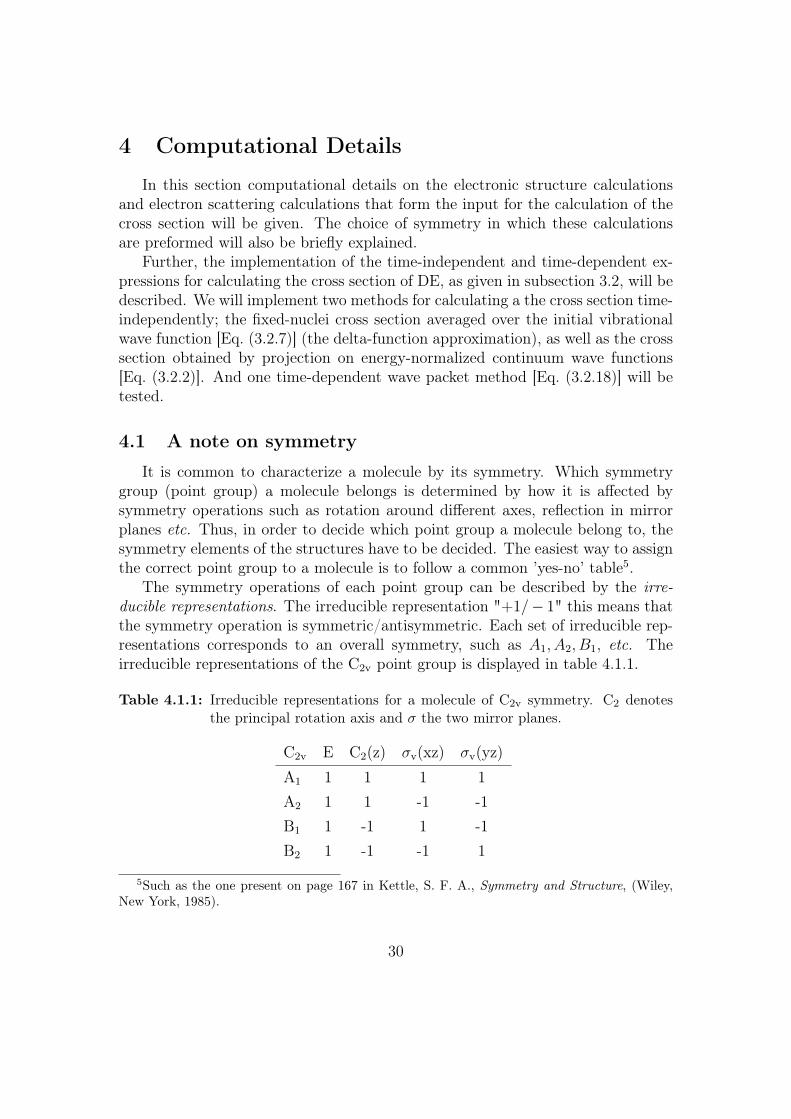
The symmetry operations of each point group can be described by the irre-ducible representations. The irreducible representation "+1/− 1" this means thatthe symmetry operation is symmetric/antisymmetric. Each set of irreducible rep-resentations corresponds to an overall symmetry, such as A1, A2, B1, etc. Theirreducible representations of the C2v point group is displayed in table 4.1.1.
Table 4.1.1: Irreducible representations for a molecule of C2v symmetry. C2 denotesthe principal rotation axis and σ the two mirror planes.
C2v E C2(z) σv(xz) σv(yz)A1 1 1 1 1A2 1 1 -1 -1B1 1 -1 1 -1B2 1 -1 -1 1
5Such as the one present on page 167 in Kettle, S. F. A., Symmetry and Structure, (Wiley,New York, 1985).
30
The HeH+ molecule is linear and does not have inversion symmetry. Thismeans that we should assign it the C∞v point group. However, this means thatthe HeH+ molecule has an infinite number of irreducible representations. There-fore, we have assigned the molecule the C2v point group for all computationalpurposes. Thus there will be four possible symmetries; A1, A2, B1 and B2. TheΣ+ in C∞v symmetry corresponds A1 symmetry, the Σ− corresponds to A2. Thetwo components of the Π-states will fall into the the B1 and B2 symmetries, whilethe two components of the ∆-states will go into A1 and A2 etc.. Since B1 and B2
will give identical contribution we only need to calculate one of them and includeit twice in the final result.
4.2 Structure calculations
The electronic structure calculations were performed using the aug-cc-pVQZ [19]basis set for He and the aug-cc-pVTZ [20] basis set for H. One extra diffuse d-functions was also added on He, resulting in a total of 106 functions.
Using these basis sets a SCF calculation on the ionic ground state was per-formed. Then a full CI calculation was preformed on the three lowest excitedstates of the ion. From the full CI, natural orbitals are computed.
All the possible excitations of the three electrons within the ten lowest naturalorbitals form the reference configurations for the MRCI calculation. Additionalsingle external excitations are also included.
4.3 Electron scattering calculations
The electron scattering calculations, using CKVM [10], are performed in A1,A2 and B1 symmetries, using the same target wave functions as the ones usedin the MRCI calculations. Scattering is calculated at the following internucleardistances R (in a0):
R = 1.0, 1.1, 1.2, 1.25, 1.3, 1.35, 1.4, 1.45, 1.5
1.55, 1.6, 1.7, 1.8, 1.9, 2.0, 2.1, 2.2, 2.3,
2.4, 2.5, 2.6, 2.7, 2.8, 3.0, 3.2, 3.4, 3.6, 3.8.
The energy interval of the scattering calculations is spanning from 15 eV to 38.9eV in steps of 0.1 eV.
From each calculation the total fixed-nuclei elastic and inelastic scattering crosssections, T -matrices etc. are obtained. The size of the T-matrices are connected tothe number of open channels, i.e the energy, and the number of (`,m)-pairs thatare included in the calculation. If N (`,m)-pairs are included in the calculation,and only one channel is open, then the size of the T-matrix is N ×N . For higher
31
energies, when two or three channels are open, the size of the T-matrix will doubleand triple, respectively.
The electron scattering calculations for the respective symmetries were per-formed for the following (`,m)-pairs:
A1 : (`,m) = (0, 0), (1, 0), (2, 0), (3, 0), (4, 0)
(5, 0), (6, 0), (2,−2), (3,−2), (4,−2)
(5,−2), (6,−2), (4,−4), (5,−4), (6,−4)
A2 : (`,m) = (2, 2), (3, 2), (4, 2), (5, 2), (6, 2)
B1 : (`,m) = (1,−1), (2,−1), (3,−1), (3,−3)
(4,−1), (4,−3), (5,−1), (5,−3), (6,−1)
(6,−3)
Thus, in the present study scattering with partial wave with ` ≤ 6, |m| ≤ 4 areincluded.
4.4 Wave packet calculations
In the time-dependent expression for the cross section of DE, wave packetpropagation is used, as described by Eq. (3.2.18). The initial condition made upof the v = 0 vibrational wave function and a T-matrix element [see Eq. (3.2.11)].
As the purpose is to test if the cross section of the DE of HeH+ can be calcu-lated using our suggested time-dependent model, this calculation will be performedonly for a simple model system where the the two first T-matrix elements in B1
symmetry for the X1Σ+ → a3Σ+ transition are included. This result will be anindication of the feasibility of the model.
The parameters giving the best convergence are dr = 0.01 and dt = 0.12(see Appendix II - Convergence testing of the wave packet model). The wavepacket is then propagated for 3000 time steps, using a propagation method basedon the Crank-Nicholson method [18].
4.5 Time-independent calculations
As there is a previous theoretical result [2] of the cross section of HeH+ obtainedtime-independently, it is meaningful to compute this quantity and compare theresults. It is also interesting to compare the different approaches to calculate thetime-independent cross section. Within the scope of this project we have chosento implement two different methods to compute the cross section of DE time-independently.
32
The expression given by Eq. (3.2.7) will give a total cross section averagedover the initial vibrational wave function. It was presented in the work of Orelet al. and here the fixed-nuclei excitation cross sections, calculated according toEq. (3.2.1), are used. In this method we have to make the delta-function approx-imation described in subsection 3.2. Nevertheless, as the fixed-nuclei excitationcross sections are available from the scattering calculation output, this methodhas the advantage that we do not have to use the T-matrix elements directly.This greatly reduces the amount of data that has to be used in the calculation.Therefore, we can obtain the total time-independent cross section according toEq. (3.2.17).
This method will also be implemented using only the first two T-matrix el-ements in B1 symmetry. Thus obtaining a partial cross section only for thesetwo elements. We do this in order to compare with the cross section obtainedtime-dependently.
An alternative way, is to use Eq. (3.2.2), where the cross section is obtained byprojection on the energy-normalized continuum wave functions [Eq. (3.2.3)]. Here,the individual T-matrix elements are also used directly, however, because of theprojection on the eigenstates of the continuum wave function it means we avoidmaking a delta-function approximation. Using this method, we will calculate apartial the cross section in B1 symmetry, and compare this result with the resultobtained from the time-dependent model.
33
5 Results
5.1 Fixed-nuclei cross section
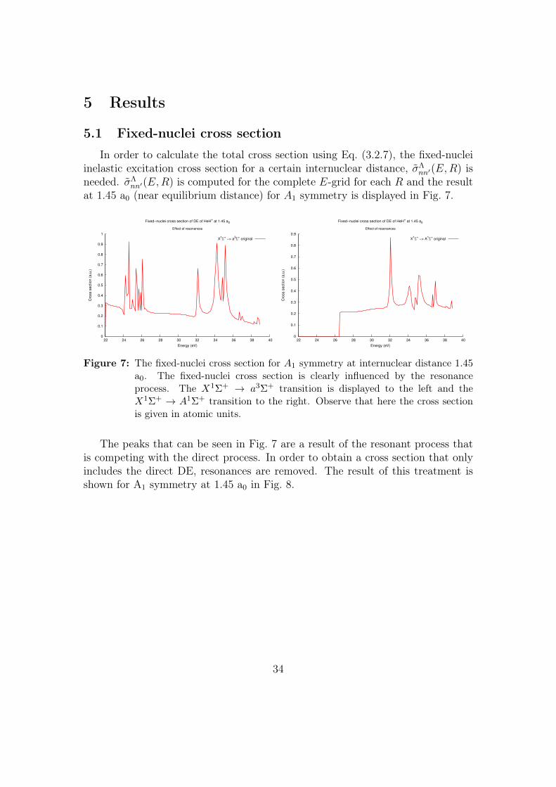
In order to calculate the total cross section using Eq. (3.2.7), the fixed-nucleiinelastic excitation cross section for a certain internuclear distance, σΛ
nn′(E,R) isneeded. σΛ
nn′(E,R) is computed for the complete E-grid for each R and the resultat 1.45 a0 (near equilibrium distance) for A1 symmetry is displayed in Fig. 7.
0
0.1
0.2
0.3
0.4
0.5
0.6
0.7
0.8
0.9
1
22 24 26 28 30 32 34 36 38 40
Cro
ss s
ectio
n (
a.u
.)
Energy (eV)
Fixed−nuclei cross section of DE of HeH+ at 1.45 a0
Effect of resonances
X1Σ
+ −> a
3Σ
+ original
0
0.1
0.2
0.3
0.4
0.5
0.6
0.7
0.8
0.9
22 24 26 28 30 32 34 36 38 40
Cro
ss s
ectio
n (
a.u
.)
Energy (eV)
Fixed−nuclei cross section of DE of HeH+ at 1.45 a0
Effect of resonances
X1Σ
+ −> A
1Σ
+ original
Figure 7: The fixed-nuclei cross section for A1 symmetry at internuclear distance 1.45a0. The fixed-nuclei cross section is clearly influenced by the resonanceprocess. The X1Σ+ → a3Σ+ transition is displayed to the left and theX1Σ+ → A1Σ+ transition to the right. Observe that here the cross sectionis given in atomic units.
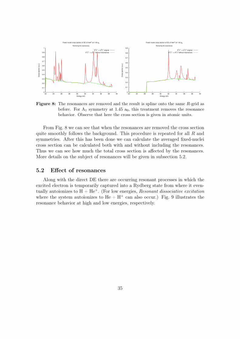
The peaks that can be seen in Fig. 7 are a result of the resonant process thatis competing with the direct process. In order to obtain a cross section that onlyincludes the direct DE, resonances are removed. The result of this treatment isshown for A1 symmetry at 1.45 a0 in Fig. 8.
34
0
0.1
0.2
0.3
0.4
0.5
0.6
0.7
0.8
0.9
1
22 24 26 28 30 32 34 36 38 40
Cro
ss s
ectio
n (
a.u
.)
Energy (eV)
Fixed−nuclei cross section of DE of HeH+ at 1.45 a0
Removing the resonances
X1Σ
+ −> a
3Σ
+ original
X1Σ
+ −> a
3Σ
+ without resonances
0
0.1
0.2
0.3
0.4
0.5
0.6
0.7
0.8
0.9
22 24 26 28 30 32 34 36 38 40
Cro
ss s
ectio
n (
a.u
.)
Energy (eV)
Fixed−nuclei cross section of DE of HeH+ at 1.45 a0
Removing the resonances
X1Σ
+ −> A
1Σ
+ original
X1Σ
+ −> A
1Σ
+ without resonances
Figure 8: The resonances are removed and the result is spline onto the same R-grid asbefore. For A1 symmetry at 1.45 a0, this treatment removes the resonancebehavior. Observe that here the cross section is given in atomic units.
From Fig. 8 we can see that when the resonances are removed the cross sectionquite smoothly follows the background. This procedure is repeated for all R andsymmetries. After this has been done we can calculate the averaged fixed-nucleicross section can be calculated both with and without including the resonances.Thus we can see how much the total cross section is affected by the resonances.More details on the subject of resonances will be given in subsection 5.2.
5.2 Effect of resonances
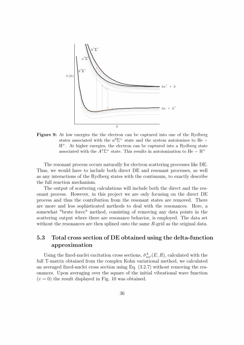
Along with the direct DE there are occurring resonant processes in which theexcited electron is temporarily captured into a Rydberg state from where it even-tually autoionizes to H + He+. (For low energies, Resonant dissociative excitationwhere the system autoionizes to He + H+ can also occur.) Fig. 9 illustrates theresonance behavior at high and low energies, respectively.
35
R
a3Σ+
X1Σ+
A1Σ+
He + H+
He+ + H
U(R)
Figure 9: At low energies the the electron can be captured into one of the Rydbergstates associated with the a3Σ+ state and the system autoionizes to He +H+. At higher energies, the electron can be captured into a Rydberg stateassociated with the A1Σ+ state. This results in autoionization to He + H+
The resonant process occurs naturally for electron scattering processes like DE.Thus, we would have to include both direct DE and resonant processes, as wellas any interactions of the Rydberg states with the continuum, to exactly describethe full reaction mechanism.
The output of scattering calculations will include both the direct and the res-onant process. However, in this project we are only focusing on the direct DEprocess and thus the contribution from the resonant states are removed. Thereare more and less sophisticated methods to deal with the resonances. Here, asomewhat "brute force" method, consisting of removing any data points in thescattering output where there are resonance behavior, is employed. The data setwithout the resonances are then splined onto the same R-grid as the original data.
5.3 Total cross section of DE obtained using the delta-functionapproximation
Using the fixed-nuclei excitation cross sections, σΛnn′(E,R), calculated with the
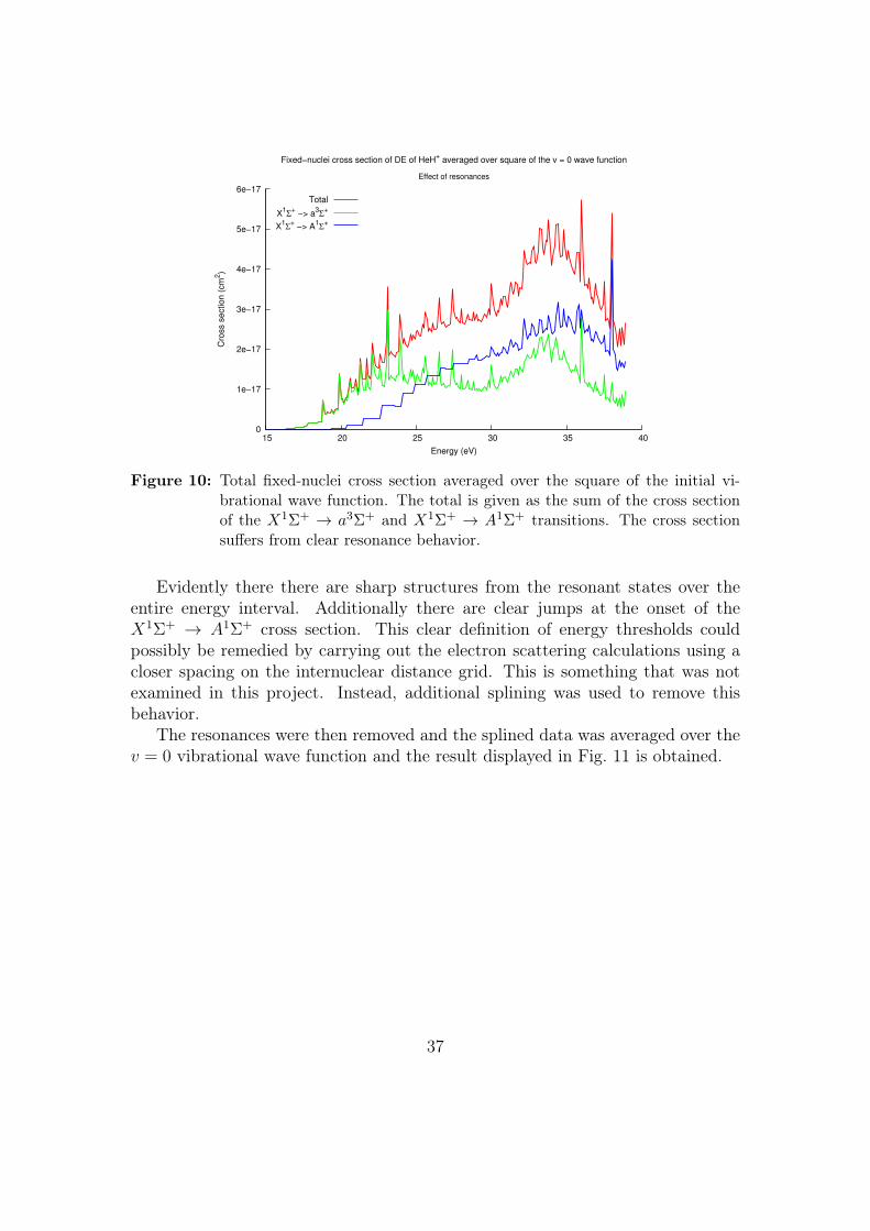
full T-matrix obtained from the complex Kohn variational method, we calculatedan averaged fixed-nuclei cross section using Eq. (3.2.7) without removing the res-onances. Upon averaging over the square of the initial vibrational wave function(v = 0) the result displayed in Fig. 10 was obtained.
36
0
1e−17
2e−17
3e−17
4e−17
5e−17
6e−17
15 20 25 30 35 40
Cro
ss s
ection (
cm
2)
Energy (eV)
Fixed−nuclei cross section of DE of HeH+ averaged over square of the v = 0 wave function
Effect of resonances
Total
X1Σ
+ −> a
3Σ
+
X1Σ
+ −> A
1Σ
+
Figure 10: Total fixed-nuclei cross section averaged over the square of the initial vi-brational wave function. The total is given as the sum of the cross sectionof the X1Σ+ → a3Σ+ and X1Σ+ → A1Σ+ transitions. The cross sectionsuffers from clear resonance behavior.
Evidently there there are sharp structures from the resonant states over theentire energy interval. Additionally there are clear jumps at the onset of theX1Σ+ → A1Σ+ cross section. This clear definition of energy thresholds couldpossibly be remedied by carrying out the electron scattering calculations using acloser spacing on the internuclear distance grid. This is something that was notexamined in this project. Instead, additional splining was used to remove thisbehavior.
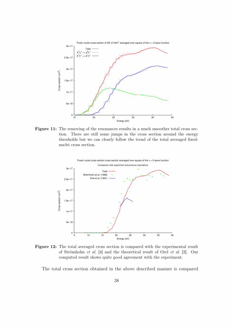
The resonances were then removed and the splined data was averaged over thev = 0 vibrational wave function and the result displayed in Fig. 11 is obtained.
37
0
5e−18
1e−17
1.5e−17
2e−17
2.5e−17
3e−17
15 20 25 30 35 40
Cro
ss s
ection (
cm
2)
Energy (eV)
Fixed−nuclei cross section of DE of HeH+ averaged over square of the v = 0 wave function
Total
X1Σ
+ −> a
3Σ
+
X1Σ
+ −> A
1Σ
+
Figure 11: The removing of the resonances results in a much smoother total cross sec-tion. There are still some jumps in the cross section around the energythresholds but we can clearly follow the trend of the total averaged fixed-nuclei cross section.
0
5e−18
1e−17
1.5e−17
2e−17
2.5e−17
3e−17
5 10 15 20 25 30 35 40
Cro
ss s
ection (
cm
2)
Energy (eV)
Fixed−nuclei cross section cross section averaged over square of the v = 0 wave function
Comparison with experiment and previous calculations
Total
Strömholm et al. (1996)
Orel et al. (1991)
Figure 12: The total averaged cross section is compared with the experimental resultof Strömholm et al. [4] and the theoretical result of Orel et al. [2]. Ourcomputed result shows quite good agreement with the experiment.
The total cross section obtained in the above described manner is compared
38
with the experimental result of Strömholm et al. [4] in Fig 12. We can see thatour theoretical result shows quite good agreement with the experimental result.
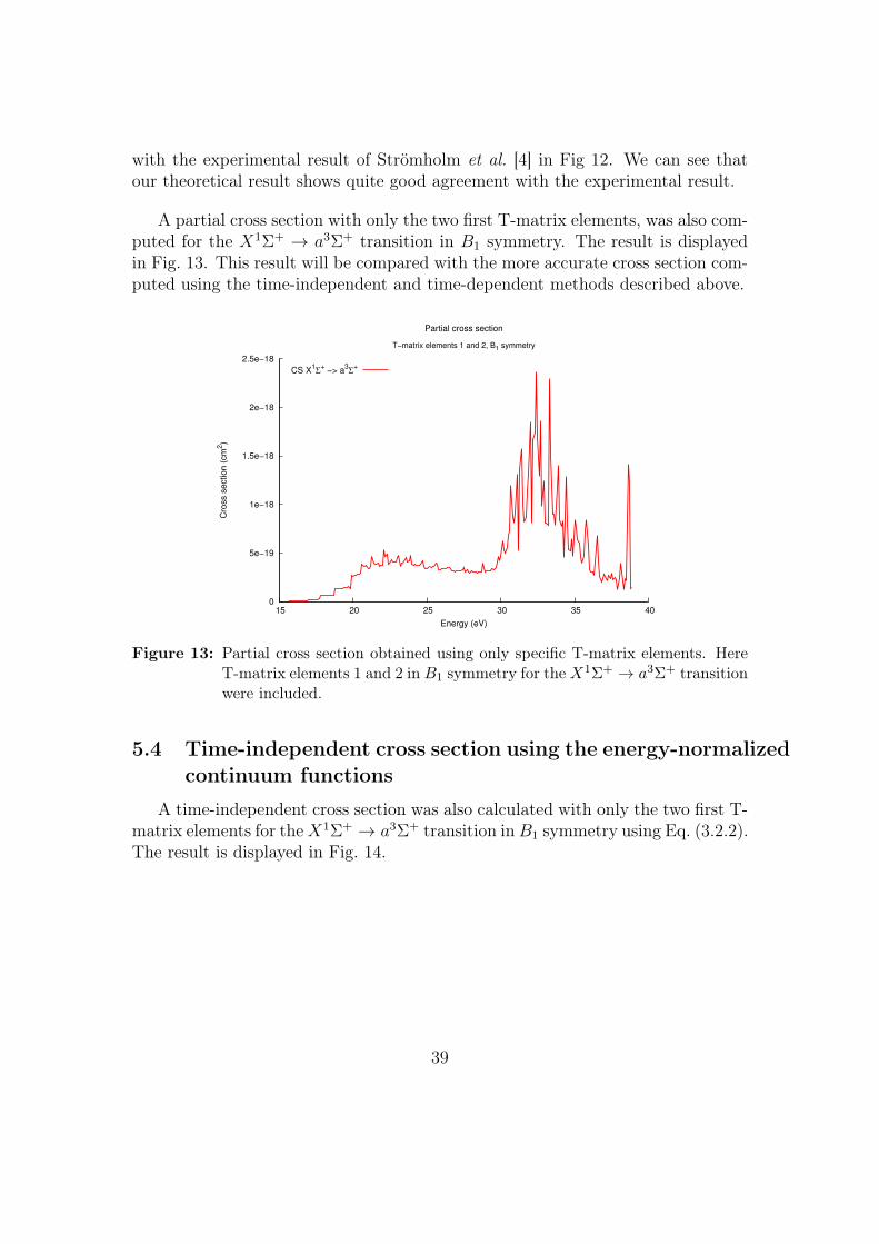
A partial cross section with only the two first T-matrix elements, was also com-puted for the X1Σ+ → a3Σ+ transition in B1 symmetry. The result is displayedin Fig. 13. This result will be compared with the more accurate cross section com-puted using the time-independent and time-dependent methods described above.
0
5e−19
1e−18
1.5e−18
2e−18
2.5e−18
15 20 25 30 35 40
Cro
ss s
ection (
cm
2)
Energy (eV)
Partial cross section
T−matrix elements 1 and 2, B1 symmetry
CS X1Σ
+ −> a
3Σ
+
Figure 13: Partial cross section obtained using only specific T-matrix elements. HereT-matrix elements 1 and 2 in B1 symmetry for theX1Σ+ → a3Σ+ transitionwere included.
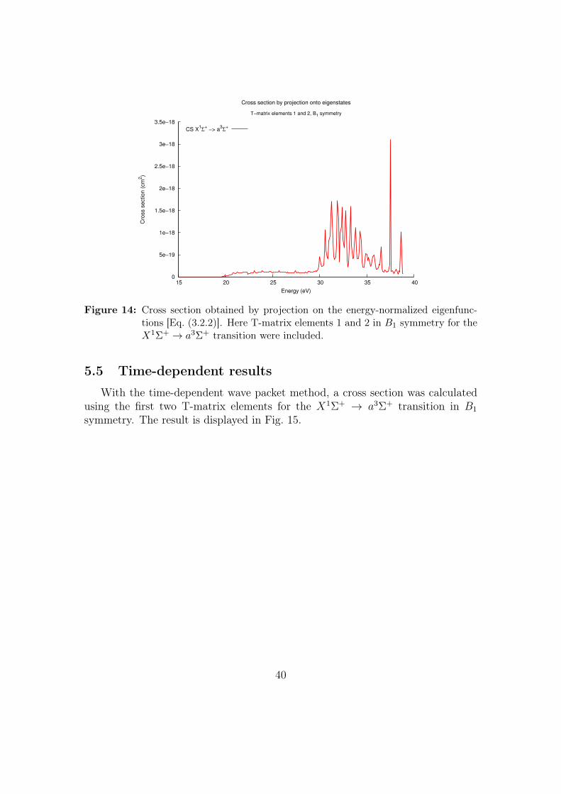
5.4 Time-independent cross section using the energy-normalizedcontinuum functions
A time-independent cross section was also calculated with only the two first T-matrix elements for theX1Σ+ → a3Σ+ transition inB1 symmetry using Eq. (3.2.2).The result is displayed in Fig. 14.
39
0
5e−19
1e−18
1.5e−18
2e−18
2.5e−18
3e−18
3.5e−18
15 20 25 30 35 40
Cro
ss s
ection (
cm
2)
Energy (eV)
Cross section by projection onto eigenstates
T−matrix elements 1 and 2, B1 symmetry
CS X1Σ
+ −> a
3Σ
+
Figure 14: Cross section obtained by projection on the energy-normalized eigenfunc-tions [Eq. (3.2.2)]. Here T-matrix elements 1 and 2 in B1 symmetry for theX1Σ+ → a3Σ+ transition were included.
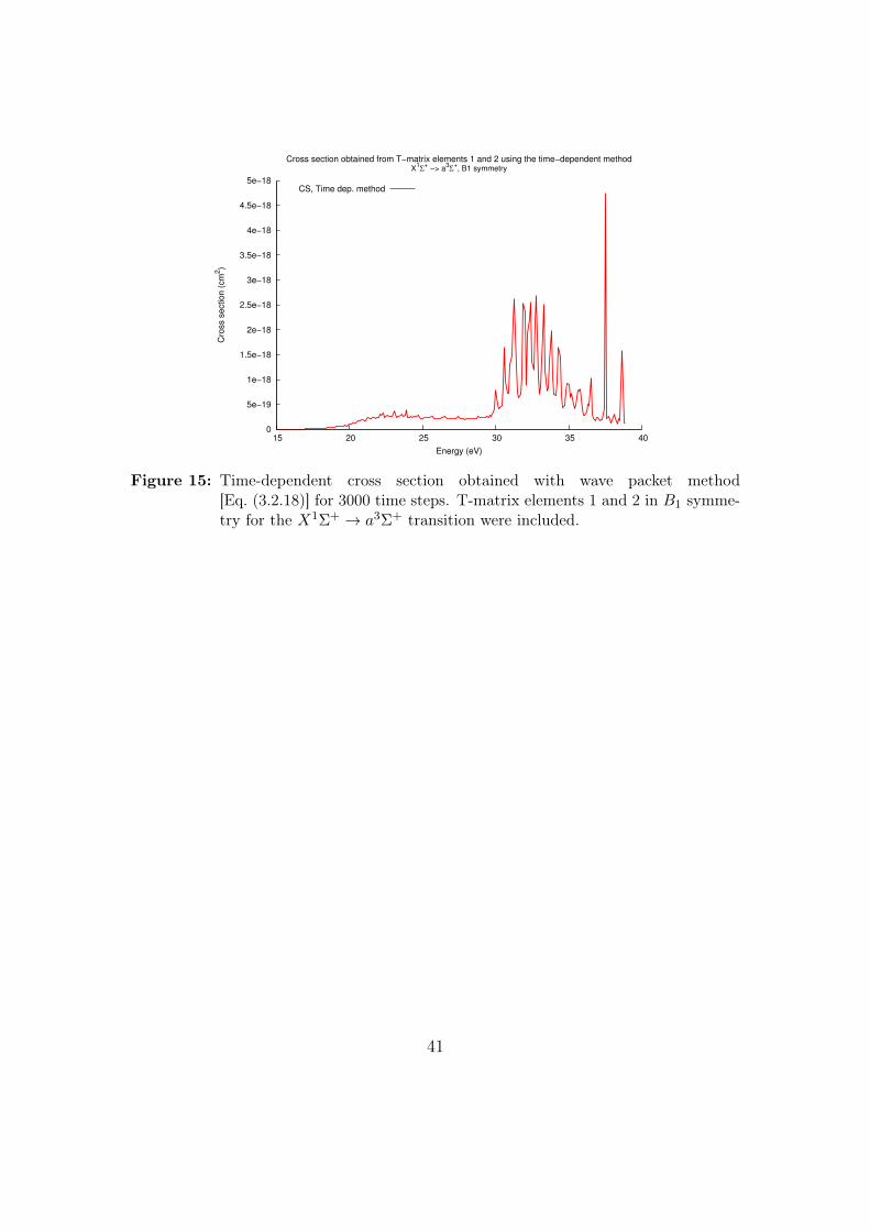
5.5 Time-dependent results
With the time-dependent wave packet method, a cross section was calculatedusing the first two T-matrix elements for the X1Σ+ → a3Σ+ transition in B1
symmetry. The result is displayed in Fig. 15.
40
0
5e−19
1e−18
1.5e−18
2e−18
2.5e−18
3e−18
3.5e−18
4e−18
4.5e−18
5e−18
15 20 25 30 35 40
Cro
ss s
ection (
cm
2)
Energy (eV)
Cross section obtained from T−matrix elements 1 and 2 using the time−dependent methodX
1Σ
+ −> a
3Σ
+, B1 symmetry
CS, Time dep. method
Figure 15: Time-dependent cross section obtained with wave packet method[Eq. (3.2.18)] for 3000 time steps. T-matrix elements 1 and 2 in B1 symme-try for the X1Σ+ → a3Σ+ transition were included.
41
5.6 Comparison of time-dependent and time-independentmethods
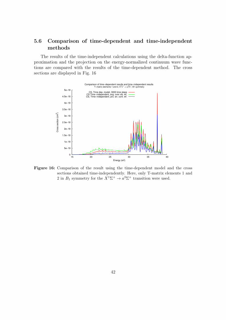
The results of the time-independent calculations using the delta-function ap-proximation and the projection on the energy-normalized continuum wave func-tions are compared with the results of the time-dependent method. The crosssections are displayed in Fig. 16
0
5e−19
1e−18
1.5e−18
2e−18
2.5e−18
3e−18
3.5e−18
4e−18
4.5e−18
5e−18
15 20 25 30 35 40
Cro
ss s
ection (
cm
2)
Energy (eV)
Comparison of time−dependent results and time−independent results T−matrix elements 1 and 2, X
1Σ
+ −> a
3Σ
+, B1 symmetry
CS, Time dep. model, 3000 time stepsCS Time−independent, avg. over vib. wf.CS, Time−independent, pro. en. cont. wf.
Figure 16: Comparison of the result using the time-dependent model and the crosssections obtained time-independently. Here, only T-matrix elements 1 and2 in B1 symmetry for the X1Σ+ → a3Σ+ transition were used.
42
6 Discussion
7 Concluding Remarks
7.1 Further applications of method
A Appendix I
A.1 Fourier transformation
Fourier transformation is a useful tool when dealing with functions such asthe Delta function and the Autocorrelation function. Therefore, it makes sense tointroduce the Fourier transform before presenting the details of any these functions.The Fourier transform of the function f(t) is defined in terms of the angularfrequency, ω, in the following manner
f(ω) =
∫ ∞−∞
f(t)e−iωtdt. (A.1.1)
An abbreviated formulation using the Fourier operator is given as
f(ω) = Ff(t). (A.1.2)
For a function f(t) fulfilling the condition of being piecewise continuos and rapidlydecaying to 0 as |t| → ∞ the Eq. A.1.1 is defined for all ω ∃ R. An inverse Fouriertransform, i.e. moving from ω-space back to t-space, is defined as follows
f(t) =1
2π
∫ ∞−∞
f(ω)eiωtdω. (A.1.3)
Eq. (A.1.3) can also be expressed using the Fourier operator in the following man-ner
f(t) = F−1f(ω). (A.1.4)
An important property of the Fourier transform is the Convolution theorem. Ifthe convolution integral is defined as
f ∗ g =
∫ ∞−∞
f(t′)g(t− t′)dt′, (A.1.5)
the Fourier transform of Eq. (A.1.5) is given as
Ff ∗ g = f(ω)g(ω). (A.1.6)
43
In principle, taking the Fourier transform of the convolution integral is the same astaking the Fourier transform of the individual functions separately. The proof ofthe Convolution theorem will be presented after the delta function is introduced.From Eq. (A.1.6) the inverse transformation follows trivially. Making the variablesubstitution ξ = t− t′ it can be found that Eq. (A.1.5) is commutative.∫ ∞
−∞f(t′ − ξ)g(ξ)dξ = g ∗ f (A.1.7)
Another useful feature of the Fourier transform is given by the Fourier integraltheorem,
f(t′) =1
2π
∫ ∞−∞
e−iωt′dω
∫ ∞−∞
f(t)eiωtdt. (A.1.8)
Eq. (A.1.8) is developed from the Fourier series and its derivation can be founde.g. in chapter 15 of Arfken & Weber [21].
A.2 The Dirac delta function
The Dirac delta function can be defined in a general manner by [22]∫ ∞−∞
f(t)δ(t− t′)dt = f(t′) (A.2.1)
and ∫ ∞−∞
δ(t)dt = 1. (A.2.2)
In the case where t′ = 0 Eq. (A.2.1) becomes∫ ∞−∞
f(t)δ(t)dt = f(0). (A.2.3)
The Fourier transform of the delta function is very useful and it is used severaltimes in this work. It is derived from the Fourier Integral (Eq. (A.1.8)) where theorder of integration has been reversed leading to the following expression,
f(t′) =
∫ ∞−∞
f(t)
[1
2π
∫ ∞−∞
eiω(t−t′)dω
]dt. (A.2.4)
Following the definition of the delta function, given in Eq. (A.2.1) it is trivial tosee that,
δ(t− t′) =1
2π
∫ ∞−∞
eiω(t−t′)dω. (A.2.5)
44
For a more detailed derivation of Eq. (A.2.5) see e.g. chapter 15 Arfken & We-ber [21].
The usefulness of the delta function will now be illustrated in the proof of theconvolution theorem presented in Eq. (A.1.6) [17]. Starting by taking the inverseFourier transform of RHS of Eq. (A.1.6) and expressing f and g also using theinverse Fourier transform the following expression is obtained
F−1f(ω)g(ω)
=
1
2π
∫ ∞−∞
∫ ∞−∞
f(t′)eiωt′dt′∫ ∞
−∞g(t′′)eiωt
′′dt′′eiωtdω.
(A.2.6)By rearranging the order of integration we get
F−1f(ω)g(ω)
=
∫ ∞−∞
∫ ∞−∞
f(t′)g(t′′)
(1
2π
∫ ∞−∞
eiω(t−(t′+t′′))dω
)dt′dt′′. (A.2.7)
Using Eq. (A.2.5) the following expression is obtained
F−1f(ω)g(ω)
=
∫ ∞−∞
∫ ∞−∞
f(t′)g(t′′)δ(t− (t′ + t′′))dt′dt′′, (A.2.8)
Thus by Eq. (A.2.1)
F−1f(ω)g(ω)
=
∫ ∞−∞
f(t′)g(t− t′)dt′ (A.2.9)
A.3 The autocorrelation function
The autocorrelation function, A(t), is convenient to use due to its connection withthe spectra of the wave packet σ(ω). The autocorrelation function is defined inthe following manner
A(t) = 〈Ψ(0)|Ψ(t)〉, (A.3.1)
and it describes the overlap between the initial wave packet and the wave packetafter a time t. By expressing the wave packet is given by the solutions for thebound state problem,
Ψ(x, t) =∑n
cnψn(x)e−iEnt. (A.3.2)
The spectrum of the wave packet is defined as
σ(ω) =∑n
|cn|2δ(ω − ω0), (A.3.3)
where ωn = En. The spectrum also can be obtained as the Fourier transform ofthe autocorrelation of the wave packet,
σ(ω) =1
2π
∫ ∞−∞
A(t)eiωtdt. (A.3.4)
45
This connection between the spectrum and the autocorrelation function can beproven in the following manner [17]:
σ(ω) =1
2π
∫ ∞−∞〈Ψ(0)|Ψ(t)〉eiωtdt (A.3.5)
By substituting Eq. (A.3.2) into Eq. (A.3.5) we obtain
σ(ω) =1
2π
∫ ∞−∞
∫ ∞−∞
(∑m
c∗mψ∗m(x)
)(∑m
cne−iEntψn(x)
)dx eiωtdt
=1
2π
∫ ∞−∞
∑m,n
c∗mcnδmne−iEnteiωtdt
=1
2π
∑n
|cn|2∫ ∞−∞
e−iEnteiωtdt = using Eq. (A.2.5)
=∑n
|cn|2δ (ω − En)
=∑n
|cn|2δ (ω − ω0)
(A.3.6)
It can be proven that the autocorrelation of the wave packet and the photodis-sociation cross section, too, are connected through a Fourier transform (see Theorysubsection 3.1).
46
B Appendix II - Convergence testing of the wavepacket model
The quality of the result of the wave packet propagation will not only relyon the input from the scattering calculations, but it will also be dependent onthe numerical stability of the calculations. One way to obtain numerically stablecalculations is to test the convergence of the numerical variables. The numericalvariables for which we have tested the convergence of the model are: the stepsize on the R-grid, dr, and the time step size, dt. dr and dt is tested prior tointroduction of the T-matrix elements, using an higher order vibrational wavefunction (v = 5, as it was the most sensitive to the numerical instability). Nowthe results of the convergence testing will be summarized.
The results of the convergence testing of the autocorrelation function and thecorresponding cross section (i.e. the Fourier transform of overlap of the v = 5vibrational wave function and the propagated wave function) for variation of dtare presented in Fig. 17.
47
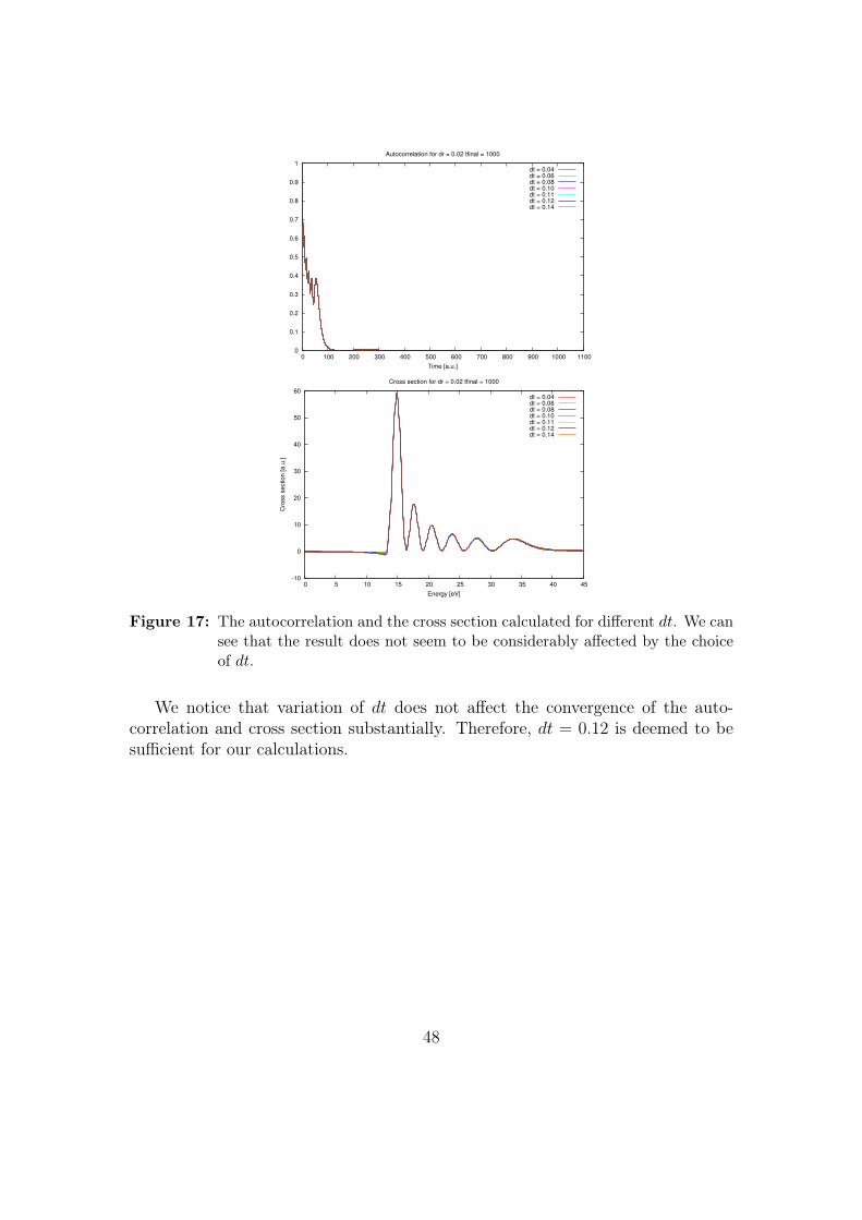
0
0.1
0.2
0.3
0.4
0.5
0.6
0.7
0.8
0.9
1
0 100 200 300 400 500 600 700 800 900 1000 1100
Time [a.u.]
Autocorrelation for dr = 0.02 tfinal = 1000
dt = 0.04dt = 0.06dt = 0.08dt = 0.10dt = 0.11dt = 0.12dt = 0.14
-10
0
10
20
30
40
50
60
0 5 10 15 20 25 30 35 40 45
Cro
ss s
ection [a.u
.]
Energy [eV]
Cross section for dr = 0.02 tfinal = 1000
dt = 0.04dt = 0.06dt = 0.08dt = 0.10dt = 0.11dt = 0.12dt = 0.14
Figure 17: The autocorrelation and the cross section calculated for different dt. We cansee that the result does not seem to be considerably affected by the choiceof dt.
We notice that variation of dt does not affect the convergence of the auto-correlation and cross section substantially. Therefore, dt = 0.12 is deemed to besufficient for our calculations.
48
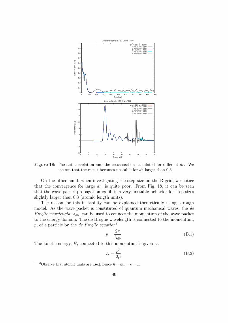
0
0.1
0.2
0.3
0.4
0.5
0.6
0.7
0.8
0.9
1
0 100 200 300 400 500 600 700 800 900 1000
Auto
corr
ela
tion [a.u
.]
Time [a.u.]
Auto correlation for dt = 0.11, tfinal = 1000
dr = 0.005, nr = 10000dr = 0.01, nr = 5000dr = 0.02, nr = 2500dr = 0.03, nr = 1666dr = 0.04, nr = 1250dr = 0.05, nr = 1000
-20
-10
0
10
20
30
40
50
60
0 5 10 15 20 25 30 35 40 45
Cro
ss s
ection [a.u
.]
Energy [eV]
Cross section dt = 0.11, tfinal = 1000
dr = 0.005, nr = 10000dr = 0.01, nr = 5000dr = 0.02, nr = 2500dr = 0.03, nr = 1666dr = 0.04, nr = 1250dr = 0.05, nr = 1000
Figure 18: The autocorrelation and the cross section calculated for different dr. Wecan see that the result becomes unstable for dr larger than 0.3.
On the other hand, when investigating the step size on the R-grid, we noticethat the convergence for large dr, is quite poor. From Fig. 18, it can be seenthat the wave packet propagation exhibits a very unstable behavior for step sizesslightly larger than 0.3 (atomic length units).
The reason for this instability can be explained theoretically using a roughmodel. As the wave packet is constituted of quantum mechanical waves, the deBroglie wavelength, λdb, can be used to connect the momentum of the wave packetto the energy domain. The de Broglie wavelength is connected to the momentum,p, of a particle by the de Broglie equation6
p =2π
λdb, (B.1)
The kinetic energy, E, connected to this momentum is given as
E =p2
2µ, (B.2)
6Observe that atomic units are used, hence ~ = me = e = 1.
49
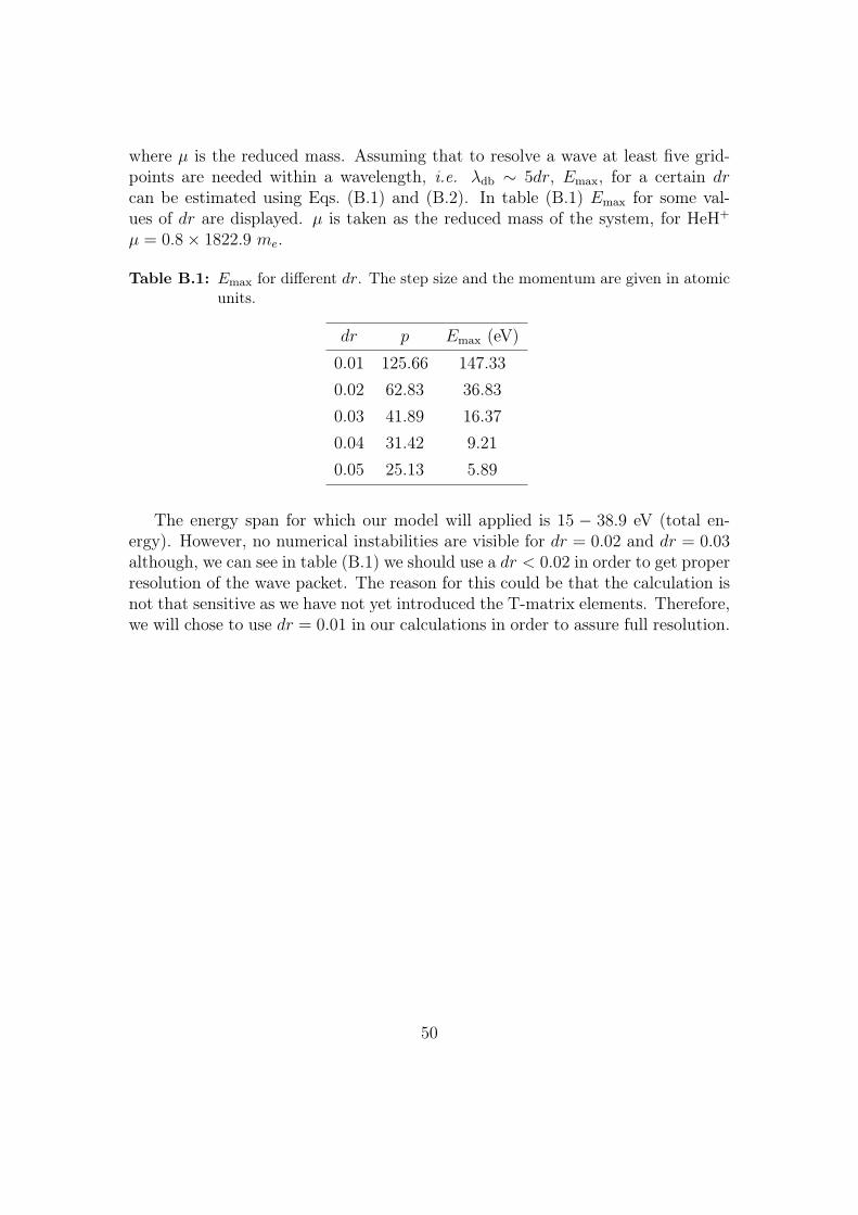
where µ is the reduced mass. Assuming that to resolve a wave at least five grid-points are needed within a wavelength, i.e. λdb ∼ 5dr, Emax, for a certain drcan be estimated using Eqs. (B.1) and (B.2). In table (B.1) Emax for some val-ues of dr are displayed. µ is taken as the reduced mass of the system, for HeH+
µ = 0.8× 1822.9 me.
Table B.1: Emax for different dr. The step size and the momentum are given in atomicunits.
dr p Emax (eV)0.01 125.66 147.330.02 62.83 36.830.03 41.89 16.370.04 31.42 9.210.05 25.13 5.89
The energy span for which our model will applied is 15 − 38.9 eV (total en-ergy). However, no numerical instabilities are visible for dr = 0.02 and dr = 0.03although, we can see in table (B.1) we should use a dr < 0.02 in order to get properresolution of the wave packet. The reason for this could be that the calculation isnot that sensitive as we have not yet introduced the T-matrix elements. Therefore,we will chose to use dr = 0.01 in our calculations in order to assure full resolution.
50
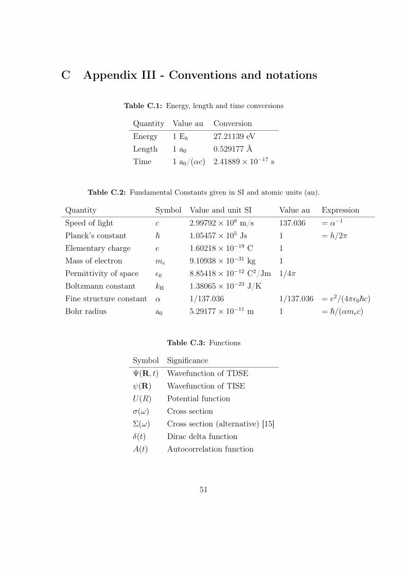
C Appendix III - Conventions and notations
Table C.1: Energy, length and time conversions
Quantity Value au ConversionEnergy 1 Eh 27.21139 eVLength 1 a0 0.529177 ÅTime 1 a0/(αc) 2.41889× 10⁻¹⁷ s
Table C.2: Fundamental Constants given in SI and atomic units (au).
Quantity Symbol Value and unit SI Value au ExpressionSpeed of light c 2.99792× 10⁸ m/s 137.036 = α−1
Planck’s constant ~ 1.05457× 10⁵ Js 1 = h/2π
Elementary charge e 1.60218× 10⁻¹⁹ C 1
Mass of electron me 9.10938× 10⁻³¹ kg 1
Permittivity of space ε0 8.85418× 10⁻¹² C2/Jm 1/4π
Boltzmann constant kB 1.38065× 10⁻²³ J/KFine structure constant α 1/137.036 1/137.036 = e2/(4πε0~c)Bohr radius a0 5.29177× 10⁻¹¹ m 1 = ~/(αmec)
Table C.3: Functions
Symbol SignificanceΨ(R, t) Wavefunction of TDSEψ(R) Wavefunction of TISEU(R) Potential functionσ(ω) Cross sectionΣ(ω) Cross section (alternative) [15]δ(t) Dirac delta functionA(t) Autocorrelation function
51
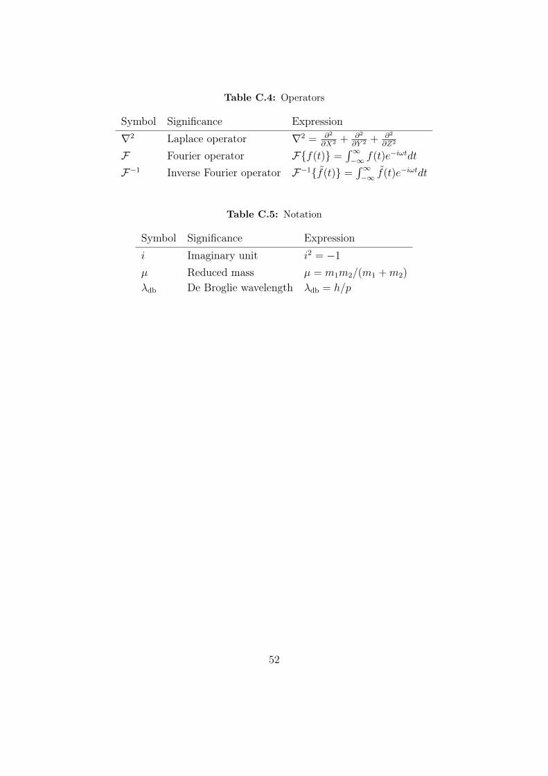
Table C.4: Operators
Symbol Significance Expression∇2 Laplace operator ∇2 = ∂2
∂X2 + ∂2
∂Y 2 + ∂2
∂Z2
F Fourier operator Ff(t) =∫∞−∞ f(t)e−iωtdt
F−1 Inverse Fourier operator F−1f(t) =∫∞−∞ f(t)e−iωtdt
Table C.5: Notation
Symbol Significance Expressioni Imaginary unit i2 = −1
µ Reduced mass µ = m1m2/(m1 +m2)
λdb De Broglie wavelength λdb = h/p
52
References
[1] M. Larsson and A. E. Orel, Dissociative Recombination of Molecular Ions(Cambridge University Press, New York, 2008), first edition, pp. 288-293.
[2] A. E. Orel, T. N. Rescigno and B. H. Lengsfield III, Phys. Rev. A 44, 4328(1991).
[3] F. B. Yousif and J. B. A. Mitchell, Phys. Rev. A 40, 4318 (1989).
[4] C. Strömholm, J. Semaniak, S. Rosen, H. Danared, S. Datz, W. van der Zandeand M. Larsson, Phys. Rev. A 54, 3086 (1996).
[5] A. E. Orel and K. C. Kulander, Phys. Rev. A 54, 4992 (1996).
[6] J. Royal and A. E. Orel, Phys. Rev. A 75, 052706 (2007).
[7] D. M. Chase, Phys. Rev. 104, 838 (1971).
[8] D. E. Golden, N. F. Lane, A. Temkin and E. Gerjuoy, Rev. Mod. Phys. 43,642 (1971).
[9] M. Shugard and A. U. Hazi, Phys. Rev. A 12, 1895 (1975).
[10] T. N. Rescigno, C. W. McCurdy, A. E. Orel and B. H. Lengsfield III, Com-putational Methods for Electron-Molecule Collisions, ed. by W. M. Huo andF. A. Gianturco (Plenum Press, New York 1995).
[11] M. Born and R. Oppenheimer, Ann. Phys. 84 457 (1927).
[12] J. von Neumann and E. P. Wiegner, Z. Phys. 30 467 (1929).
[13] C. W. McCurdy, T. N.Rescigno and B. I. Schneider, Phys. Rev. A 36, 2061(1987).
[14] B. I. Schneider and T. N. Rescigno, Phys. Rev. A, 37, 3749 (1988).
[15] E. J. Heller, J. Chem. Phys. 68, 2066 (1978).
[16] E. J. Heller, J. Chem. Phys. 68, 3891 (1978).
[17] D. J. Tannor, Introduction to quantum mechanics, a time-dependent perspec-tive (University Science Books, Sausalito, CA, 2007), first edition.
[18] A. Goldberg, H. M. Shey and J. L. Schwartz, Am. J. Phys. 35, 177(1967).
53
[19] D. E Woon and T. H. Dunning, Jr., J. Chem. Phys. 100, 2975 (1994).
[20] T. H. Dunning, Jr., J. Chem. Phys. 90, 1007 (1989).
[21] G. B. Arfken and H. J. Weber, Mathematical methods for physicists (ElsevierAcademic Press, Burlington, MA, 2005), sixth edition.
[22] A. Prosperetti, Advanced Mathematics for Applications (Cambridge Univer-sity Press, New York, 2011), first edition.
54


 with OH[sup −](H[sub 2]O)[sub 1,2] clusters](https://img.pdfslide.net/doc/110x75/632533d67fd2bfd0cb0356e7/dissociative-excitation-transfer-in-the-reaction-of-osub-2asup-1dsub-g.jpg)


