A two-fluid model for violent aerated flows

Frederic Dias ∗, Denys Dutykh1 and Jean-Michel Ghidaglia

Centre de Mathematiques et de Leurs Applications,ENS Cachan and CNRS, UniverSud, 61 avenue du President Wilson,

F-94235 Cachan Cedex, and LRC MESO, ENS Cachan, CEA DAM DIF1 Now at Universite de Savoie, Laboratoire de Mathematiques LAMA - UMR 5127

Campus Scientifique, 73376 Le Bourget-du-Lac Cedex.

Abstract

In the study of ocean wave impact on structures, one often uses Froude scaling sincethe dominant force is gravity. However the presence of trapped or entrained air inthe water can significantly modify wave impacts. When air is entrained in water inthe form of small bubbles, the acoustic properties in the water change dramatically.While some work has been done to study small-amplitude disturbances in suchmixtures, little work has been done on large disturbances in air-water mixtures. Wepropose a basic two-fluid model in which both fluids share the same velocities andanalyze some of its properties. It is shown that this model can successfully mimicwater wave impacts on coastal structures. The governing equations are discretizedby a second-order finite volume method. Numerical results are presented for twoexamples: the dam break problem and the drop test problem. The results suggestthat this basic model can be used to study violent aerated flows, especially byproviding fast qualitative estimates.

Key words: free-surface flow, wave impact, two-phase flow, compressible flow,finite volumes

1 Introduction

One of the challenges in Computational Fluid Dynamics (CFD) is to deter-mine efforts exerted by waves on structures, especially coastal structures. The

∗ Corresponding author.Email addresses: Frederic.Dias@cmla.ens-cachan.fr (Frederic Dias),

Denys.Dutykh@cmla.ens-cachan.fr (Denys Dutykh1),jmg@cmla.ens-cachan.fr (Jean-Michel Ghidaglia).

Preprint submitted to Computers and Fluids 3 July 2009

hal-0

0285

037,

ver

sion

3 -

3 Ju

l 200

9

flows associated with wave impact can be quite complicated. In particular,wave breaking can lead to flows that cannot be described by models like e.g.the free-surface Euler or Navier–Stokes equations. In a free-surface model, theboundary between the gas (air) and the liquid (water) is a surface. The liq-uid flow is assumed to be incompressible, while the gas is represented by amedium, above the liquid, in which the pressure is constant (the atmosphericpressure in general). Such a description is known to be valid for calculatingthe propagation in the open sea of waves with moderate amplitude, which donot break. Clearly it is not satisfactory when waves either break or hit coastalstructures like offshore platforms, jetties, piers, breakwaters, etc.

Our goal here is to investigate a relatively simple two-fluid model that canhandle breaking waves. It belongs to the family of averaged models, in thesense that even though the two fluids under consideration are not miscible,there exists a length scale ǫ such that each averaging volume (of size ǫ3) con-tains representative samples of each of the fluids. Once the averaging process isperformed, it is assumed that the two fluids share, locally, the same pressure,temperature and velocity. Such models are called homogeneous models in theliterature. They can be seen as limiting cases of more general two-fluid modelswhere the fluids can have different temperatures and velocities [13]. Let usexplain why it can be assumed here that both fluids share the same temper-atures and velocities. There are relaxation mechanisms that indeed tend tolocally equalize these two quantities. Concerning temperatures, these are dif-fusion processes and provided no phenomenon is about to produce very stronggradients of temperature between the two fluids like e.g. a nuclear reaction inone of the two fluids, one can assume that the time scale on which diffusionacts is much smaller than the time scale on which the flow is averaged. Sim-ilarly, concerning the velocities, drag forces tend to locally equalize the twovelocities. Define a time scale built on the mean convection velocity and atypical length scale. For flows in which the mean convection velocity is mod-erate, this time scale based on convection is much larger than the time scaleon which velocities are equalized through turbulent drag forces. Hence, in thepresent model, the partial differential equations, which express conservationof mass (1 per fluid), balance of momentum and total energy, read as follows:

(α+ρ+)t + ∇ · (α+ρ+~u)= 0, (1)

(α−ρ−)t + ∇ · (α−ρ−~u)= 0, (2)

(ρ~u)t + ∇ · (ρ~u ⊗ ~u + pI)= ρ~g, (3)

(ρE)t + ∇ · (ρH~u)= ρ~g · ~u, (4)

where the superscripts ± are used to denote liquid and gas respectively. Henceα+ and α− denote the volume fraction of liquid and gas, respectively, andsatisfy the condition α+ + α− = 1. We denote by ρ±, ~u, p, e respectively thedensity of each phase, the velocity, the pressure, the specific internal energy,

2

hal-0

0285

037,

ver

sion

3 -

3 Ju

l 200

9

~g is the acceleration due to gravity (in two space dimensions, ~g is equal to(0,−g)), ρ := α+ρ+ + α−ρ− is the total density, E = e + 1

2|~u|2 is the specific

total energy, H := E + p/ρ is the specific total enthalpy. In order to closethe system, we assume that the pressure p is given as a function of threeparameters, namely α ≡ α+ − α−, ρ and e:

p = P(α, ρ, e) . (5)

We shall discuss in Section 2 how such a function P is determined once the twoindependent equations of state p = P±(ρ±, e±) are known. Equations (1)–(5)form a closed system that we shall use to simulate aerated flows.

The main purpose of this paper is to promote a general point of view, whichmay be useful for various applications dealing with violent aerated flows inocean, offshore, coastal and arctic engineering. We do not consider here un-derwater explosions, where the word violent has a different meaning. The det-onation of an explosive charge underwater results in an initial high-velocityshockwave through the water, in movement or displacement of the water itselfand in the formation of a high-pressure bubble of high-temperature gas. Thisbubble expands rapidly until it either vents to the surface or until its internalpressure is exceeded by that of the water surrounding it [15]. What we dois to follow the approach first used, we believe, by the late Howell Peregrineand his collaborators [3,17,16]. The influence of the presence of air in waveimpacts is a difficult topic. While it is usually thought that the presence ofair softens the impact pressures, recent results show that the cushioning effectdue to aeration via the increased compressibility of the air-water mixture isnot necessarily a dominant effect [4]. First of all, air may become trappedor entrained in the water in different ways, for example as a single bubbletrapped against a wall, or as a column or cloud of small bubbles. In addition,it is not clear which quantity is the most appropriate to measure impacts. Forexample some researchers pay more attention to the pressure impulse thanto pressure peaks. The pressure impulse is defined as the integral of pressureover the short duration of impact. A long time ago, Bagnold [1] noticed thatthe maximum pressure and impact duration differed from one identical waveimpact to the next, even in carefully controlled laboratory experiments, whilethe pressure impulse appears to be more repeatable. For sure, the simple one-fluid models which are commonly used for examining the peak impacts are nolonger appropriate in the presence of air. There are few studies dealing withtwo-fluid models. An exception is the work by Peregrine and his collaborators.Wood et al. [21] used the pressure impulse approach to model a trapped airpocket. Peregrine & Thais [18] examined the effect of entrained air on a partic-ular kind of violent water wave impact by considering a filling flow. Bullock etal. [5] found pressure reductions when comparing wave impact between freshand salt water, due to the different properties of the bubbles in the two fluids.Indeed the aeration levels are much higher in salt water than in fresh water.

3

hal-0

0285

037,

ver

sion

3 -

3 Ju

l 200

9

Bredmose [2] recently performed numerical experiments on a two-fluid systemwhich has similarities with the one we will use below.

The novelty of the present paper is not the finite volume method used belowbut rather the modelling of two-fluid flows. Since the model described belowdoes not involve the tracking nor the capture of a free surface, its integration ischeap from the computational point of view. We have chosen to report here onthe case of inviscid flow. Should the viscosity effects become important, theycan be taken into account via e.g. a fractional step method. In fact, whenviscous effects are important, the flow is easier to capture from the numericalpoint of view.

The paper is organized as follows. Section 2 provides an analytical study ofthe model. Section 3 deals with numerical simulations based on this modelvia a finite volume method. Two examples are shown: the dam break problemand the drop test problem. Finally a conclusion ends the paper.

2 Analytical study of the model

2.1 The extended equation of state

It is shown in this section how to determine the function P(α, ρ, e) in Eq. (5)once the two equations of state p = P±(ρ±, e±) are known. We call Eq. (5) anextended EOS, since P(−1, ρ, e) = P−(ρ, e) and P(1, ρ, e) = P+(ρ, e), where

p± = P±(ρ±, e±) , T± = T ±(ρ±, e±) , (6)

are the EOS of each fluid, with T± the temperature of each phase. Althoughour approach is totally general, we will use the following prototypical examplein this paper. Assume that the fluid denoted by the superscript − is an idealgas:

p− = (γ− − 1)ρ−e−, e− = C−V T−, (7)

while the fluid denoted by the superscript + obeys the stiffened gas law [6,11]:

p+ + π+ = (γ+ − 1)ρ+e+, e+ = C+V T+ +

π+

γ+ρ+, (8)

where γ±, C±V , and π+ are constants. For example, pure water is well described

in the vicinity of the normal conditions by taking γ+ = 7 and π+ = 2.1 × 109

Pa.

Let us now return to the general case. In order to find the function P, thereare three given quantities: α ∈ [−1, 1] , ρ > 0 and e > 0 . Then one solves forthe four unknowns ρ± , e± the following system of four nonlinear equations:

4

hal-0

0285

037,

ver

sion

3 -

3 Ju

l 200

9

(1 + α)ρ+ + (1 − α)ρ− =2ρ , (9)

(1 + α)ρ+e+ + (1 − α)ρ−e− =2ρ e , (10)

P+(ρ+, e+) −P−(ρ−, e−) = 0 , (11)

T +(ρ+, e+) − T −(ρ−, e−) = 0 . (12)

For given values of the pressure p > 0 and the temperature T > 0, we denoteby R±(p, T ) and E±(p, T ) the solutions (ρ±, e±) to:

P±(ρ±, e±) = p , T ±(ρ±, e±) = T , (13)

and then:

ρ =1 + α

2R+(p, T ) +

1 − α

2R−(p, T ) , (14)

ρ e =1 + α

2R+(p, T ) E+(p, T ) +

1 − α

2R−(p, T ) E−(p, T ) . (15)

Finally the inversion of this system of equations leads to p = P(α, ρ, e) andT = T (α, ρ, e).

Remark 1 The system (1)–(4), (7)-(8) and (13) is a differential and alge-braic equation, while the system (1)–(5) is a partial differential equation as itis the case for a system of single fluid equations.

Concerning the prototypical case, the following generalization of (7) is consid-ered:

p− + π− = (γ− − 1)ρ−e−, e− = C−V T− +

π−

γ−ρ−. (16)

This generalization, which has the additional parameter π−, allows one to setthe speed of sound to a certain value independently of γ−, p− and ρ−. Usingcomputer algebra to invert (14) and (15) leads to the following expressions:

P(α, ρ, e) = (γ(α) − 1)ρ e − π(α) , (17)

T (α, ρ, e)=ρ e − (λ+(α)π+ + λ−(α)π−)

ρ CV (α), (18)

where the five functions γ(α), π(α), CV (α) and λ±(α) are defined by

5

hal-0

0285

037,

ver

sion

3 -

3 Ju

l 200

9

2

γ(α) − 1=

1 + α

γ+ − 1+

1 − α

γ− − 1, (19)

2 π(α)

γ(α) − 1=

1 + α

γ+ − 1π+ +

1 − α

γ− − 1π− , (20)

(

1 + α

C+V (γ+ − 1)

+1 − α

C−V (γ− − 1)

)

CV (α) =1 + α

γ+ − 1+

1 − α

γ− − 1, (21)

λ±(α)≡1 ± α

2(γ± − 1)

(

1 −CV (α)

γ±C±V

)

. (22)

One can easily check that one recovers the equations of state for each fluid inthe limits α → ±1. Note that similar expressions can be found in Section 1.1of [12] where a two-dimensional, compressible, two-fluid mathematical modelwas used to compute numerically wave breaking.

2.2 A hyperbolic system of conservation laws

In this section, we assume that the system of equations is solved in R2, having

in mind the numerical computations performed below. However the extensionto 3D is straightforward. The system (1)–(4) can be written as

∂w

∂t+ ∇ · F(w) = S(w) , (23)

wherew = (wi)

5i=1 := (α+ρ+, α−ρ−, ρu1, ρu2, ρE) , (24)

and, for every ~n ∈ R2,

F(w) ·~n = (α+ρ+~u ·~n, α−ρ−~u ·~n, ρ~u ·~nu1 +pn1, ρ~u ·~nu2 +pn2, ρH~u ·~n) , (25)

S(w) = (0, 0, ρg1, ρg2, ρ~g · ~u) . (26)

The Jacobian matrix A(w) · ~n is defined by

A(w) · ~n =∂(F(w) · ~n)

∂w. (27)

In order to compute A(w) · ~n, one writes Eq. (25) for F(w) · ~n in terms of w

and p:

F(w) · ~n =(

w1w3n1 + w4n2

w1 + w2, w2

w3n1 + w4n2

w1 + w2, w3

w3n1 + w4n2

w1 + w2+ pn1,

w4w3n1 + w4n2

w1 + w2+ pn2, (w5 + p)

w3n1 + w4n2

w1 + w2

)

. (28)

6

hal-0

0285

037,

ver

sion

3 -

3 Ju

l 200

9

The Jacobian matrix (27) then has the following expression:

A(w) · ~n =

unα−ρ−

ρ−un

α+ρ+

ρα+ρ+

ρn1

α+ρ+

ρn2 0

−unα−ρ−

ρun

α+ρ+

ρα−ρ−

ρn1

α−ρ−

ρn2 0

−u1un + ∂p∂w1

n1 −u1un + ∂p∂w2

n1 un + u1n1 + ∂p∂w3

n1 u1n2 + ∂p∂w4

n1∂p

∂w5n1

−u2un + ∂p∂w1

n2 −u2un + ∂p∂w2

n2 u2n1 + ∂p∂w3

n2 un + u2n2 + ∂p∂w4

n2∂p

∂w5n2

un

(

∂p

∂w1− H

)

un

(

∂p

∂w2− H

)

un∂p

∂w3+ Hn1 un

∂p

∂w4+ Hn2 un

(

1 + ∂p

∂w5

)

,

where un = ~u · ~n.

Let us now compute the five derivatives ∂p/∂wi. A systematic way of doing itis to introduce a set of five independent physical variables and here we shalltake:

ϕ1 = α, ϕ2 = p, ϕ3 = T, ϕ4 = u1, ϕ5 = u2 . (29)

The expressions of the w′is in terms of the ϕ′

js are algebraic and explicit.Hence the Jacobian matrix ∂wi/∂ϕj can be easily computed. Since ∂ϕj/∂wi

is its inverse matrix, one finds easily with the help of a computer algebraprogram that

∂p

∂w1

=Γ − 1

2(u2

1 + u22) + α−ρ−χ− , (30)

∂p

∂w2

=Γ − 1

2(u2

1 + u22) + α+ρ+χ+ , (31)

∂p

∂w3= −(Γ − 1)u1 ,

∂p

∂w4= −(Γ − 1)u2 ,

∂p

∂w5= Γ − 1 , (32)

where

χ∓ =1

ρ±

(c∓s )2

γ∓ − 1−

1

ρ∓

(c±s )2

γ± − 1, χ+ + χ− = 0 , (33)

(c±s )2 ≡ C±V γ±(γ± − 1)T =

γ±p + π±

ρ±, (34)

Γ − 1 ≡ (γ(α) − 1)ρc2

s

γ(α)p + π(α). (35)

In Eq. (35), we have introduced the speed of sound of the mixture cs, definedby

1

ρc2s

=(1 + α)γ+

2ρ+(c+s )2

+(1 − α)γ−

2ρ−(c−s )2−

1

ρa2, (36)

with

ρa2 ≡(1 + α)ρ+(c+

s )2

2(γ+ − 1)+

(1 − α)ρ−(c−s )2

2(γ− − 1). (37)

7

hal-0

0285

037,

ver

sion

3 -

3 Ju

l 200

9

Then one can show that the Jacobian matrix A(w) · ~n has three distincteigenvalues:

λ1 = un − cs, λ2,3,4 = un, λ5 = un + cs, (38)

These three eigenvalues are real and there is a complete set of real valuedeigenvectors. The expressions of these eigenvectors can be obtained by usinga computer algebra program.

Remark 2 If π+ = 0 and π− = 0, then c2s = γ(α)p

ρand a2 = c2

s

γ(α)−1.

Remark 3 The left hand side of (36) is positive since ρa2 is bounded from

below by (1+α)ρ+(c+s

)2

2γ+ + (1−α)ρ−(c−s

)2

2γ−. Thus a2 is seen to play the role of the square

of the enthalpy by analogy with the monofluid case.

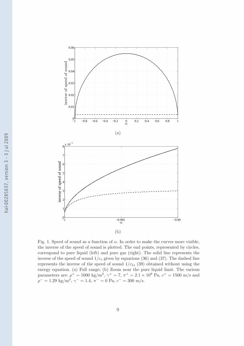
A plot of 1/cs(α) is given in Fig. 1 (see the solid line). A remarkable propertyis that the speed of sound exhibits a minimum. If the energy equation was nottaken into consideration, this minimum would not be present (see the dashedline in Fig. 1). Indeed, the expression for the speed of sound for homogeneoustwo-fluid models with the additional assumption that the flow is isentropic is

cIs =

√

√

√

√

(α−ρ+ + α+ρ−)(c+s )2(c−s )2

α+ρ−(c−s )2 + α−ρ+(c+s )2

. (39)

This expression can be found in Appendix C of [7] (see equations (C.20) and(C.21)).

2.3 Evolution equations for the physical variables

The system of conservation laws (1)–(4) can be transformed into a set ofevolution equations for the physical variables. Let us introduce the entropyfunction s(~x, t) defined by (compare with Eq. (10))

2ρ s = (1 + α)ρ+s+ + (1 − α)ρ−s−.

Proposition 1 Continuous solutions to (1)–(4) satisfy

~ut + ~u · ∇~u +1

ρ∇p =~g , (40)

pt + ~u · ∇p + ρc2s∇ · ~u = 0 , (41)

αt + ~u · ∇α + (1 − α2) δ∇ · ~u = 0 , (42)

st + ~u · ∇s= 0 , (43)

8

hal-0

0285

037,

ver

sion

3 -

3 Ju

l 200

9

−1 −0.8 −0.6 −0.4 −0.2 0 0.2 0.4 0.6 0.8 10

0.01

0.02

0.03

0.04

0.05

0.06

α

inve

rse

ofsp

eed

ofso

und

(a)

−1 −0.995 −0.990

1

2

3

4

5

6

7

8x 10

−3

α

inve

rse

of s

peed

of s

ound

(b)

Fig. 1. Speed of sound as a function of α. In order to make the curves more visible,the inverse of the speed of sound is plotted. The end points, represented by circles,correspond to pure liquid (left) and pure gas (right). The solid line represents theinverse of the speed of sound 1/cs given by equations (36) and (37). The dashed linerepresents the inverse of the speed of sound 1/cIs (39) obtained without using theenergy equation. (a) Full range; (b) Zoom near the pure liquid limit. The variousparameters are: ρ+ = 1000 kg/m3, γ+ = 7, π+ = 2.1 × 109 Pa, c+ = 1500 m/s andρ− = 1.29 kg/m3, γ− = 1.4, π− = 0 Pa, c− = 300 m/s.

9

hal-0

0285

037,

ver

sion

3 -

3 Ju

l 200

9

where c2s is given by (36)-(37) and δ is given by

δ ≡ρc2

s(γ−π+ − γ+π−)

ρ+ρ−(c+s )2(c−s )2

. (44)

Remark 4 For pure fluids (α = ±1), Eq. (42) is no longer relevant and δis not needed. One can check that the speed of sound cs is then equal to theexpected speed of sound (c+

s or c−s ) for pure fluids.

The balance of entropy (43) comes from the balance

(ρs)t + ∇ · (ρs~u) = 0. (45)

Adding together Eqs (1) and (2) leads to

ρt + ∇ · (ρ~u) = 0. (46)

Combining Eqs (45) and (46) leads to Eq. (43).

Remark 5 Subtracting Eq. (1) from Eq. (2) leads to

(ρχ)t + ∇ · (ρχ~u) = 0 , with χ =α+ρ+ − α−ρ−

ρ. (47)

In the case of smooth solutions, we obtain that

χt + ~u · ∇χ = 0 ,

which is an alternative to Eq. (42).

2.4 Pure fluid limit

The two-fluid model described in the present paper is based on the volumefraction of liquid and gas. In some situations, this volume fraction can havesharp gradients. Consider for example a tanh-type distribution of α along thevertical axis with essentially pure gas at the top, pure liquid at the bottomand a middle layer where α goes rapidly from −1 to 1. One can even considerthe limiting case where the transition is discontinuous. In this section westudy this limit and we show that the two-fluid model degenerates into theclassical water-wave equations. In other words one has an interface separatingtwo pure fluids. So the well-known water-wave equations are a by-product ofthe two-fluid system under investigation. A similar type of limit in the caseof a continuously stratified incompressible fluid degenerating into a two-layerincompressible fluid was considered by James [14].

10

hal-0

0285

037,

ver

sion

3 -

3 Ju

l 200

9

In the rest of this section, it is assumed that there are no shocks. Consider the3D case where α is either 1 or −1. More precisely let

α := 1 − 2H(z − η(~x, t)) , ~x = (x1, x2) , (48)

where H is the Heaviside step function, z the vertical coordinate and x1, x2

the horizontal coordinates. Physically this substitution means that we considertwo pure fluids separated by an interface. It follows that

α+α− = 0 , 1 − α2 = 0 .

Substituting the expression (48) into the equation (42) gives

ηt + ~uh · ∇hη = w ,

where ~uh = (u1, u2), ∇h = (∂x1, ∂x2

) and w is the vertical velocity.

This equation simply states that there is no mass flux across the interface.Incidentally this is no longer true in the case of shock waves. Integrating theconservation of momentum equation (3) inside a volume moving with the flowand enclosing the interface, and using the fact that there is no mass fluxacross the interface simply leads to the fact that there is no pressure jumpacross the interface. In other words, the pressure is continuous across theinterface. Integrating the entropy equation inside the same volume enclosingthe interface and using the fact there is no mass flux across the interface doesnot lead to any new information.

One can now write Eqs (2)–(4) in each fluid by taking α± = 1, either in theconservative form

(ρ±)t + ∇ · (ρ±~u±) = 0 , (49)

(ρ±~u±)t + ∇ · (ρ±~u± ⊗ ~u±) + ∇p± = ρ±~g , (50)

(ρ±s±)t + ∇ · (ρ±s±~u±) = 0 , (51)

(see Whitham [20] for example for the last equation) or in the more classicalform

ρ±t + (~u± · ∇)ρ± + ρ±∇ · ~u± = 0 , (52)

~u±t + (~u± · ∇)~u± +

∇p±

ρ±=~g , (53)

s±t + ~u± · ∇s± = 0 . (54)

In these two systems, the superscripts + and − are used for the heavy fluid(below the interface) and the light fluid (above the interface) respectively.

11

hal-0

0285

037,

ver

sion

3 -

3 Ju

l 200

9

The system of equations we derived is nothing else than the system of adiscontinuous two-fluid system with an interface located at z = η(~x, t). Alongthe interface, one has the kinematic and dynamic boundary conditions

ηt + ~u±h · ∇hη =w± , (55)

p− = p+ . (56)

This simple computation shows an important property of our model: it auto-matically degenerates into a discontinuous two-fluid system where two purecompressible phases are separated by an interface. This limit has interestingconsequences. In particular, interfacial flows develop waves along the interfaceand these waves are usually dispersive. Therefore one can also expect disper-sive waves to exist in the two-fluid model. Since the emphasis of the presentpaper is the study of large-amplitude disturbances, the derivation of the dis-persion relation for the two-fluid model is left for future work. Note howeverthat preliminary results can be found in [7]. Even the question of which reststate one must consider is not trivial.

3 Simulations of aerated violent flows

3.1 A finite-volume discretization of the model

Here we describe the discretization of the model (1)–(4) by a standard cell-centered finite volume method. The computational domain Ω ⊂ R

d is trian-gulated into a set of control volumes: Ω = ∪K∈T K. We start by integratingequation (23) on K:

d

dt

∫

Kw dΩ +

∑

L∈N (K)

∫

K∩LF(w) · ~nKL dσ =

∫

KS(w) dΩ , (57)

where ~nKL denotes the unit normal vector on K ∩ L pointing into L andN (K) = L ∈ T : area(K ∩ L) 6= 0 . Then, setting

wK(t) :=1

vol(K)

∫

Kw(~x, t) dΩ ,

we approximate (57) by

dwK

dt+

∑

L∈N (K)

area(L ∩ K)

vol(K)Φ(wK ,wL;~nKL) = S(wK) , (58)

12

hal-0

0285

037,

ver

sion

3 -

3 Ju

l 200

9

where the numerical flux

Φ(wK ,wL;~nKL) ≈1

area(L ∩ K)

∫

K∩LF(w) · ~nKL dσ

is explicitly computed by the FVCF formula of Ghidaglia et al. [9]:

Φ(v,w; n) =F(v) · ~n + F(w) · ~n

2− sgn(An(µ(v,w)))

F(w) · ~n − F(v) · ~n

2.

(59)Here v and w are dummy variables. The Jacobian matrix An(µ) is defined in(27), µ(v,w) is an arbitrary mean between v and w (for example µ(v,w) =(1/2)(v+w)) and sgn(M) is the matrix whose eigenvectors are those of M butwhose eigenvalues are the signs of that of M . As explained in [9], this methodis able to model discontinuities such as shock waves and sharp interfaces.

So far we have not discussed the case where a control volume K meets theboundary of Ω. Here we shall only consider the case where this boundary is awall and from the numerical point of view, we only need to find the normalflux F · ~n. Since ~u(~x, t) · ~n = 0 for ~x ∈ ∂Ω , we have

(F · ~n)|~x∈∂Ω = (0, 0, pb~n, 0), pb := p|~x∈∂Ω ,

and following Ghidaglia and Pascal [10], we can take pb = p + ρuncs, wherethe right-hand side is evaluated in the control volume K.

Remark 1 In order to turn (58) into a numerical algorithm, we must atleast perform time discretization and give an expression for µ(v,w). Sincethis matter is standard, we do not give the details here but instead refer toDutykh [8]. Let us also notice that formula (58) leads to a first-order schemebut in fact we use a MUSCL technique to achieve higher accuracy in space[19].

3.2 Numerical results

In order to check the accuracy of our second-order scheme on smooth solutionsand its robustness against discontinuous solutions, we have performed theclassical test cases for which we refer to [8]. The most famous test case is thatof Sod’s shock tube. We report here on some of the situations which havemotivated this study.

3.2.1 Thermodynamics constants

The constants C±V can be calculated after simple algebraic manipulations of

equations (7), (8) and matching with experimental values at normal condi-

13

hal-0

0285

037,

ver

sion

3 -

3 Ju

l 200

9

parameter value

p0 105 Pa

ρ+0 103 kg/m3

ρ−0 1.29 kg/m3

T0 300 K

γ− 1.4

γ+ 7

π+ 2.1 × 109 Pa

C+V 166.72 J

kg·K

C−V 646.0 J

kg·K

Table 1Values of the parameters for an air/water mixture under normal conditions.

tions:C−

V ≡p0

(γ− − 1)ρ−0 T0

,

C+V ≡

γ+p0 + π+

(γ+ − 1)γ+ρ+0 T0

.

For example, for an air/water mixture under normal conditions we have thevalues given in Table 1.

The sound velocities in each phase are given by the following formulas:

(c−s )2 =γ−p−

ρ−, (c+

s )2 =γ+p+ + π+

ρ+. (60)

In the two test cases described below, we use a very high value for the accel-eration due to gravity: g = 100 ms−2. The only motivation is to accelerate thedynamics. All results are presented with physical dimensions. For example,the 1 × 1 box used for the computations corresponds to a 1 m by 1 m box.

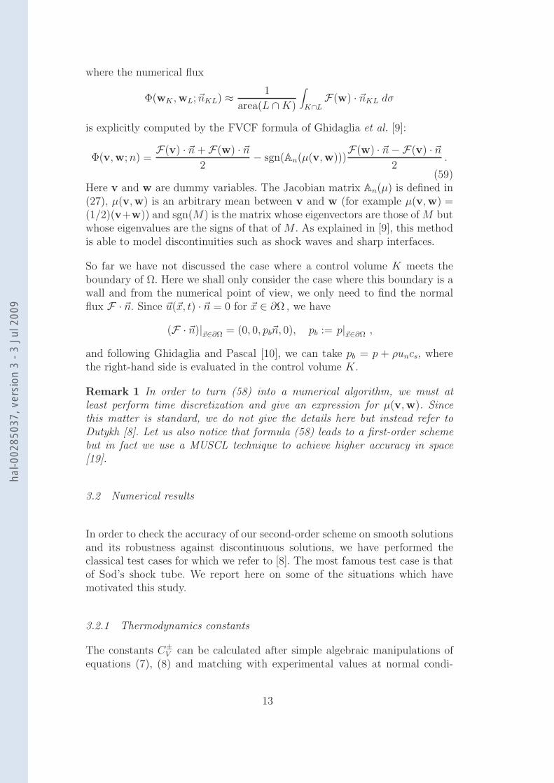
3.2.2 Falling water column

The geometry and initial condition for this test case are shown on Fig. 2.Initially the velocity field is taken to be zero. At time t = 0, the volumefraction of gas is 0.9 (white area) while the volume fraction of water is 0.9(dark area). The values of the other parameters are given in Table 1. Themesh used in this computation contained about 108000 control volumes (inthis case they were triangles). The results of this simulation are presented onFigures 3–8. Fig. 9 shows the maximal pressure on the right wall as a function

14

hal-0

0285

037,

ver

sion

3 -

3 Ju

l 200

9

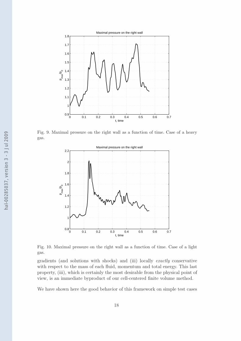
of time:

t 7−→ max(x,y)∈1×[0,1]

p(x, y, t).

We performed another computation for a mixture with α+ = 0.05, α− = 0.95.The pressure is recorded as well and plotted in Fig. 10. One can see that thepeak value is higher and the impact is more localized in time.

α+ = 0.9α− = 0.1

α+ = 0.1α− = 0.9

0 0.3 0.65 0.7

0.05

1

1

0.9

~g

Fig. 2. Falling water column test case. Geometry and initial condition. All the valuesfor α± are at time t = 0.

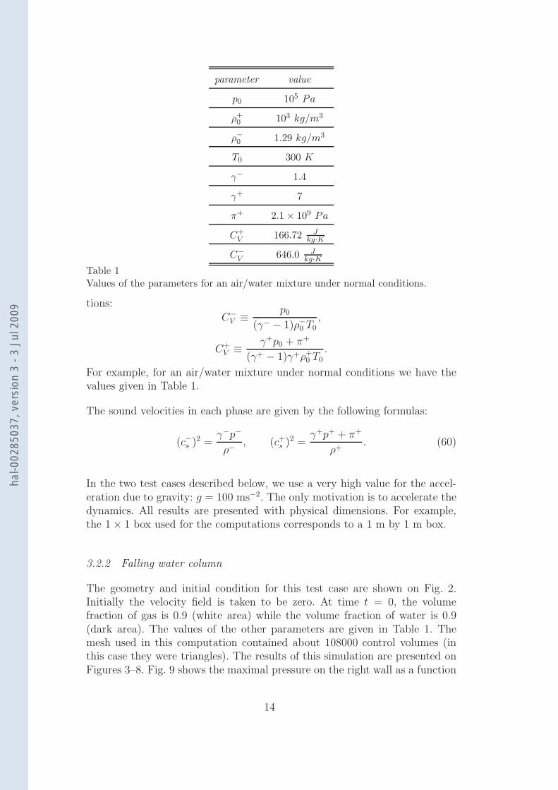
(a) t = 0.005 s (b) t = 0.06 s

Fig. 3. Falling water column test case. Initial condition and the beginning of thecolumn collapse.

15

hal-0

0285

037,

ver

sion

3 -

3 Ju

l 200

9

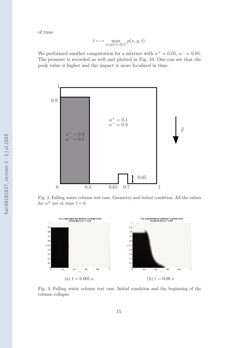
(a) t = 0.1 s (b) t = 0.125 s

Fig. 4. Falling water column test case. Splash formation due to the interaction withthe step.

(a) t = 0.15 s (b) t = 0.175 s

Fig. 5. Falling water column test case. Water hits the wall.

(a) t = 0.2 s (b) t = 0.225 s

Fig. 6. Same as Fig. 5 at later times.

3.2.3 Water drop test case

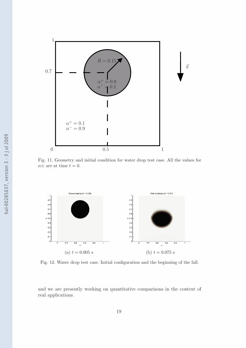
The geometry and initial condition for this test case are shown on Fig. 11.Initially the velocity field is taken to be zero. The values of the other parame-

16

hal-0

0285

037,

ver

sion

3 -

3 Ju

l 200

9

(a) t = 0.3 s (b) t = 0.4 s

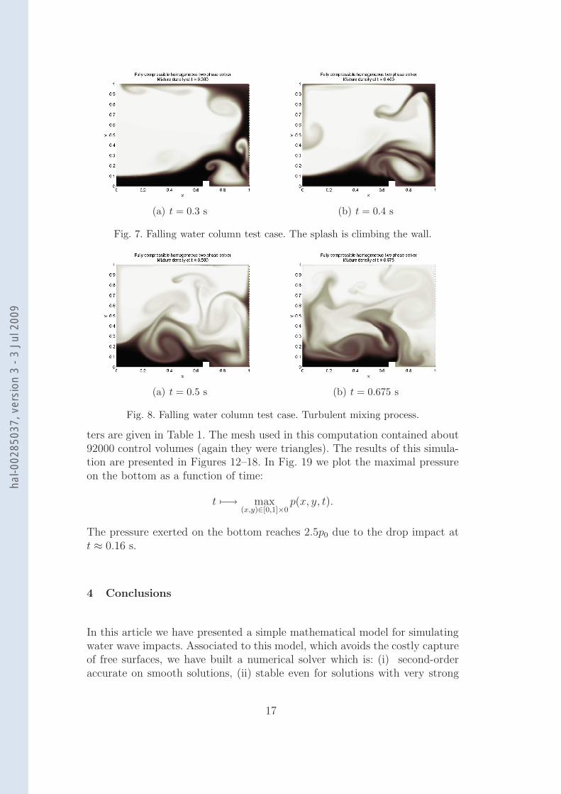
Fig. 7. Falling water column test case. The splash is climbing the wall.

(a) t = 0.5 s (b) t = 0.675 s

Fig. 8. Falling water column test case. Turbulent mixing process.

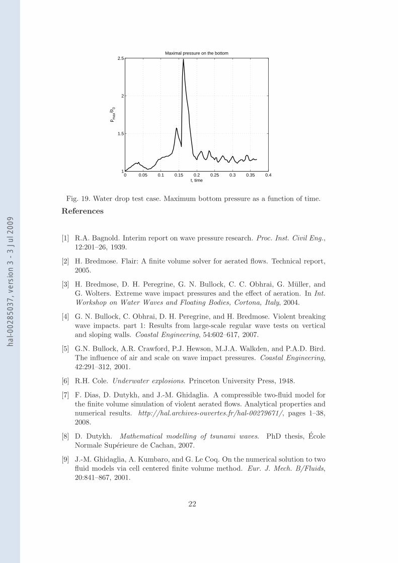
ters are given in Table 1. The mesh used in this computation contained about92000 control volumes (again they were triangles). The results of this simula-tion are presented in Figures 12–18. In Fig. 19 we plot the maximal pressureon the bottom as a function of time:

t 7−→ max(x,y)∈[0,1]×0

p(x, y, t).

The pressure exerted on the bottom reaches 2.5p0 due to the drop impact att ≈ 0.16 s.

4 Conclusions

In this article we have presented a simple mathematical model for simulatingwater wave impacts. Associated to this model, which avoids the costly captureof free surfaces, we have built a numerical solver which is: (i) second-orderaccurate on smooth solutions, (ii) stable even for solutions with very strong

17

hal-0

0285

037,

ver

sion

3 -

3 Ju

l 200

9

0 0.1 0.2 0.3 0.4 0.5 0.6 0.70.9

1

1.1

1.2

1.3

1.4

1.5

1.6

1.7

1.8

t, time

p max

/p0

Maximal pressure on the right wall

Fig. 9. Maximal pressure on the right wall as a function of time. Case of a heavygas.

0 0.1 0.2 0.3 0.4 0.5 0.6 0.70.8

1

1.2

1.4

1.6

1.8

2

2.2

t, time

p max

/p0

Maximal pressure on the right wall

Fig. 10. Maximal pressure on the right wall as a function of time. Case of a lightgas.

gradients (and solutions with shocks) and (iii) locally exactly conservativewith respect to the mass of each fluid, momentum and total energy. This lastproperty, (iii), which is certainly the most desirable from the physical point ofview, is an immediate byproduct of our cell-centered finite volume method.

We have shown here the good behavior of this framework on simple test cases

18

hal-0

0285

037,

ver

sion

3 -

3 Ju

l 200

9

α+ = 0.1α− = 0.9

α+ = 0.9α− = 0.1

0 0.5

0.7

1

1

~gR = 0.15

Fig. 11. Geometry and initial condition for water drop test case. All the values forα± are at time t = 0.

(a) t = 0.005 s (b) t = 0.075 s

Fig. 12. Water drop test case. Initial configuration and the beginning of the fall.

and we are presently working on quantitative comparisons in the context ofreal applications.

19

hal-0

0285

037,

ver

sion

3 -

3 Ju

l 200

9

(a) t = 0.1 s (b) t = 0.125 s

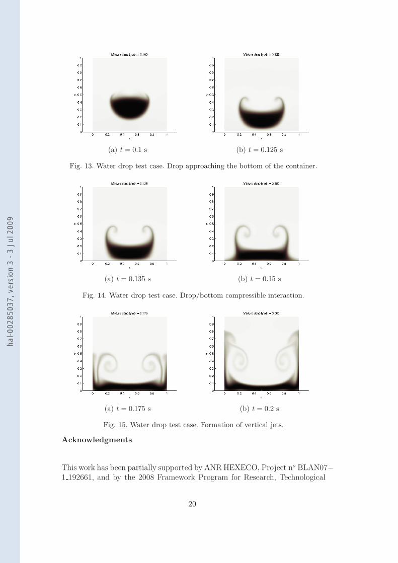
Fig. 13. Water drop test case. Drop approaching the bottom of the container.

(a) t = 0.135 s (b) t = 0.15 s

Fig. 14. Water drop test case. Drop/bottom compressible interaction.

(a) t = 0.175 s (b) t = 0.2 s

Fig. 15. Water drop test case. Formation of vertical jets.

Acknowledgments

This work has been partially supported by ANR HEXECO, Project no BLAN07−1 192661, and by the 2008 Framework Program for Research, Technological

20

hal-0

0285

037,

ver

sion

3 -

3 Ju

l 200

9

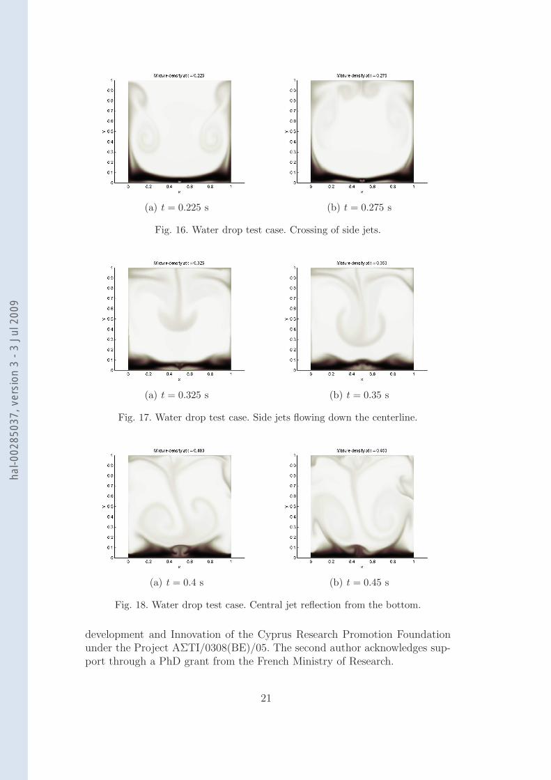
(a) t = 0.225 s (b) t = 0.275 s

Fig. 16. Water drop test case. Crossing of side jets.

(a) t = 0.325 s (b) t = 0.35 s

Fig. 17. Water drop test case. Side jets flowing down the centerline.

(a) t = 0.4 s (b) t = 0.45 s

Fig. 18. Water drop test case. Central jet reflection from the bottom.

development and Innovation of the Cyprus Research Promotion Foundationunder the Project AΣTI/0308(BE)/05. The second author acknowledges sup-port through a PhD grant from the French Ministry of Research.

21

hal-0

0285

037,

ver

sion

3 -

3 Ju

l 200

9

0 0.05 0.1 0.15 0.2 0.25 0.3 0.35 0.41

1.5

2

2.5

t, time

p max

/p0

Maximal pressure on the bottom

Fig. 19. Water drop test case. Maximum bottom pressure as a function of time.

References

[1] R.A. Bagnold. Interim report on wave pressure research. Proc. Inst. Civil Eng.,12:201–26, 1939.

[2] H. Bredmose. Flair: A finite volume solver for aerated flows. Technical report,2005.

[3] H. Bredmose, D. H. Peregrine, G. N. Bullock, C. C. Obhrai, G. Muller, andG. Wolters. Extreme wave impact pressures and the effect of aeration. In Int.Workshop on Water Waves and Floating Bodies, Cortona, Italy, 2004.

[4] G. N. Bullock, C. Obhrai, D. H. Peregrine, and H. Bredmose. Violent breakingwave impacts. part 1: Results from large-scale regular wave tests on verticaland sloping walls. Coastal Engineering, 54:602–617, 2007.

[5] G.N. Bullock, A.R. Crawford, P.J. Hewson, M.J.A. Walkden, and P.A.D. Bird.The influence of air and scale on wave impact pressures. Coastal Engineering,42:291–312, 2001.

[6] R.H. Cole. Underwater explosions. Princeton University Press, 1948.

[7] F. Dias, D. Dutykh, and J.-M. Ghidaglia. A compressible two-fluid model forthe finite volume simulation of violent aerated flows. Analytical properties andnumerical results. http://hal.archives-ouvertes.fr/hal-00279671/, pages 1–38,2008.

[8] D. Dutykh. Mathematical modelling of tsunami waves. PhD thesis, EcoleNormale Superieure de Cachan, 2007.

[9] J.-M. Ghidaglia, A. Kumbaro, and G. Le Coq. On the numerical solution to twofluid models via cell centered finite volume method. Eur. J. Mech. B/Fluids,20:841–867, 2001.

22

hal-0

0285

037,

ver

sion

3 -

3 Ju

l 200

9

[10] J.-M. Ghidaglia and F. Pascal. The normal flux method at the boundary formultidimensional finite volume approximations in cfd. European Journal ofMechanics B/Fluids, 24:1–17, 2005.

[11] S.K. Godunov, A. Zabrodine, M. Ivanov, A. Kraiko, and G. Prokopov.Resolution numerique des problemes multidimensionnels de la dynamique desgaz. Editions Mir, Moscow, 1979.

[12] P. Helluy, F. Golay, J.-P. Caltagirone, P. Lubin, S. Vincent, D. Drevard,R. Marcer, P. Fraunie, N. Seguin, S. Grilli, A.-C. Lesage, A. Dervieux, andO. Allain. Numerical simulation of wave breaking. Mathematical Modelling andNumerical Analysis, 39(3):591–607, 2005.

[13] M. Ishii. Thermo-Fluid Dynamic Theory of Two-Phase Flow. Eyrolles, Paris,1975.

[14] G. James. Internal travelling waves in the limit of a discontinuously stratifiedfluid. Arch. Rational Mech. Anal., 160:41–90, 2001.

[15] B. Le Mehaute and S. Wang. Water Waves Generated by Underwater Explosion,Advanced Series on Ocean Engineering, Vol. 10. World Scientific, Singapore,1995.

[16] D. H. Peregrine, H. Bredmose, G. Bullock, A. Hunt, and C. Obhrai. Water waveimpact on walls and the role of air. In Proc. 30th Int. Conf. Coast. Engng., SanDiego (ed. J. M. Smith), vol. 5, pp. 4494-4506. ASCE, 2006.

[17] D. H. Peregrine, H. Bredmose, G. Bullock, C. Obhrai, G. Muller, andG. Wolters. Water wave impact on walls and the role of air. In Proceedings ofthe 29th International Conference on Coastal Engineering, Lisbon 2004, vol. 4,pp. 4005-4017. ASCE, 2004.

[18] D.H. Peregrine and L. Thais. The effect of entrained air in violent water impacts.J. Fluid Mech., 325:377–97, 1996.

[19] B. van Leer. Upwind and high-resolution methods for compressible flow: Fromdonor cell to residual-distribution schemes. Communications in ComputationalPhysics, 1:192–206, 2006.

[20] G.B. Whitham. Linear and nonlinear waves. John Wiley & Sons Inc., NewYork, 1999.

[21] D.J. Wood, D.H. Peregrine, and T. Bruce. Wave impact on wall using pressure-impulse theory. i. trapped air. Journal of Waterway, Port, Coastal and OceanEngineering, 126(4):182–190, 2000.

23

hal-0

0285

037,

ver

sion

3 -

3 Ju

l 200

9