Seediscussions,stats,andauthorprofilesforthispublicationat:https://www.researchgate.net/publication/3451611

AUnifyingFrameworkforFiniteWordlengthRealizations

ArticleinCircuitsandSystemsI:RegularPapers,IEEETransactionson·September2007

DOI:10.1109/TCSI.2007.902408·Source:IEEEXplore

CITATIONS

33

READS

18

3authors,including:

ThibaultHilaire

PierreandMarieCurieUniversity-Paris6

30PUBLICATIONS157CITATIONS

SEEPROFILE

JamesWhidborne

CranfieldUniversity

210PUBLICATIONS1,546CITATIONS

SEEPROFILE

AllcontentfollowingthispagewasuploadedbyThibaultHilaireon18March2014.

Theuserhasrequestedenhancementofthedownloadedfile.Allin-textreferencesunderlinedinbluearelinkedtopublicationsonResearchGate,lettingyouaccessandreadthemimmediately.

IEEE TRANSACTIONS ON CIRCUITS AND SYSTEMS—I: REGULAR PAPERS, VOL. 54, NO. 8, AUGUST 2007 1765

A Unifying Framework for Finite WordlengthRealizations

Thibault Hilaire, Philippe Chevrel, and James F. Whidborne, Member, IEEE

Abstract—A general framework for the analysis of the finitewordlength (FWL) effects of linear time-invariant digital filterimplementations is proposed. By means of a special implicit systemdescription, all realization forms can be described. An algebraiccharacterization of the equivalent classes is provided, whichenables a search for realizations that minimize the FWL effectsto be made. Two suitable FWL coefficient sensitivity measuresare proposed for use within the framework, these being a transferfunction sensitivity measure and a pole sensitivity measure. Anillustrative example is presented.

Index Terms—Coefficient sensitivity, digital filter implementa-tion, digital filter wordlength effects, finite wordlength (FWL) ef-fects, implicit systems, optimal realization.

I. INTRODUCTION

WHEN digital filters are implemented, they are imple-mented with finite precision due to the finite wordlength

(FWL) of the representation of numbers within the computingmachine. There are two FWL effects. The first is the addition ofnoise into the system resulting from the rounding of variablesbefore and after each arithmetic operation—the “roundoffnoise.” The second is the degradation in the performanceand/or the stability resulting from rounding of the filter coef-ficients—the “coefficient sensitivity.” The FWL problem ishence to analyze the effects to ensure that they do not causesignificant deterioration in the performance of an implementedfilter. The effects are obviously dependent upon the chosenwordlength and on the chosen arithmetic format (floating-point,fixed-point, etc.). Slightly less obvious is the fact that the FWLeffects are very dependent upon the particular realization,(direct form, cascade, etc.), and upon the chosen operator (shiftoperator, operator, etc.). Thus, in seeking to alleviate the FWLeffects, the realization must also be considered.

The FWL effects have been studied for many years. Althoughmany of the early works were motivated by problems in controlsystems [1], [2], the analysis of the effects were often consideredin the open loop. See [3] for a comprehensive review of earlywork. Further reviews can be found in [4]–[6]. There has beena large amount of work that considers the problem of roundoff

Manuscript received July 10, 2006; revised November 27, 2006. This paperwas recommended by Associate Editor T. Hinamoto.

T. Hilaire is with the Institut National de Recherche en Informatique eten Automatique (INRIA), Lannion 22300, France (e-mail: thibault.hilaire@irisa.fr).

P. Chevrel is with the Institut de Recherche en Communications et Cyberné-tique de Nantes (IRCCyN), Nantes 44321, France.

J. F. Whidborne is with the Department of Aerospace Sciences, CranfieldUniversity, Cranfield MK43 0AL, U.K.

Digital Object Identifier 10.1109/TCSI.2007.902408

noise (e.g., [7]–[9]), however the emphasis of this paper is onthe coefficient sensitivity problem.

Early consideration of the transfer function sensitivity torounding errors in the coefficients can be found in [10], [11].The work of Thiele [12]–[14] is particularly important indefining a norm on the input–output sensitivity that is tractable.This sensitivity measure provides the foundation for much ofthe subsequent work. Solutions for other similar measures canbe found in [5], [15] and further developed in, for example,[16]–[18]. A related measure using a statistical analysis ofthe input–output sensitivity has been developed [19]. An ex-tension to the multivariable system case is provided in [20].The closed-loop control case has also been considered, forexample in [21]. Methods for the simultaneous minimizationof a sensitivity measure with roundoff noise [22] and subject toscaling requirements [23] have also been developed recently.

The sensitivity of the poles (and zeros) is also a commonlyused measure of the coefficient rounding effect. An early anal-ysis appears in [24]. Mantey [25] showed that the poles/eigen-values are dependent on the state-space realization. It is well-known that an eigenvalue sensitivity is minimized if the systemis normal [26]. However Gevers and Li [5] subsequently de-termined the realization that would minimize a pole sensitivitymeasure combined with a zero sensitivity measure proposed in[27]. Much subsequent work (see [28]–[31], for example) hasconsidered various similar eigenvalue sensitivity measures forclosed-loop control systems.

Most of the significant results have expressed the filter in thestate space form. Although most realizations can be transformedinto the state-space form, this form is not completely generaland has several limitations. Firstly, the analysis of the roundingeffect of a specific coefficient in a particular realization formcan become very difficult after transformation to the state spaceform. Secondly, many realization forms require the computa-tion of intermediate variables that cannot be expressed in thestate-space form. Furthermore, the state space form is specificto the chosen operator. In reality all implementable operatorsare actually implemented using the shift operator. For example,a realization expressed in the form of a -operator is actuallyimplemented using a shift operator in combination with an in-termediate variable.

Thus, a description that includes intermediate variables is re-quired. This paper proposes a particular implicit state-space de-scription that is not subject to these limitations. The proposedspecialized implicit form provides a generalized description ofany realization in a form that allows a straightforward analysisof the FWL effects as will be shown later in this paper. Thedescription is macroscopic in that it does not require coding

1549-8328/$25.00 © 2007 IEEE

1766 IEEE TRANSACTIONS ON CIRCUITS AND SYSTEMS—I: REGULAR PAPERS, VOL. 54, NO. 8, AUGUST 2007

details and is platform independent but gives a direct relation-ship between the description and the implementation algorithm.Note that the idea of representing the intermediate variables inthe description has been considered previously [32] (see also[33], [34]), but the description form is less general than the im-plicit form considered in this paper. For example, -realizationscannot be described using this form.

The paper is organized as follows. In the next section, the spe-cialized implicit form is proposed, and a number of definitionsgiven. The idea of a set of structured realizations, or structura-tion is introduced and several examples of structurations pro-vided. In Section III, the equivalence classes of a realization inthe specialized implicit form are provided. This is necessary toenable the determination of realizations that are relatively im-pervious to FWL effects. In Section IV, several coefficient sen-sitivity measures are proposed for use with the specialized im-plicit form. Some examples are given in Section V. Note thatalthough the emphasis in this paper is on the coefficient sensi-tivity problem, the proposed implicit form can be just as usefulto the analysis and solution of the roundoff noise problem, andthis will be done in future works.

II. UNIFYING FRAMEWORK

A. Specialized Implicit Form

To show the utility of the implicit realization, we consider anexample of the implementation of a -operator state-space real-ization. It is well-known [5], [35], [36] that the -operator is nu-merically superior to the usual shift operator generally resultingin less sensitive implementations with less rounding noise.

For a realization expressed with the -operator, the input/output relation is

(1)

with , where is a strictly positive constant andis the delay operator [5]. This is equivalent, in infinite precision,to the classical state-space realization

(2)

with , , and .With these two equivalent realizations, the parametrization is

different, therefore when the parameters are subjected to FWLrounding, the two realizations are no longer equivalent, and theimpact of the quantization is different. In addition, in order toimplement the -operator, intermediate variables are necessary.These are also subject to FWL quantization. So the followingalgorithm:

(3)

implements (1) where is an intermediate variable vector.There are many other possible implementation forms, such

as direct form I or II, cascade/parallel decomposition, lattice fil-ters, mixed , etc., and many of these also require interme-diate variables. In order to consider all of them within a general

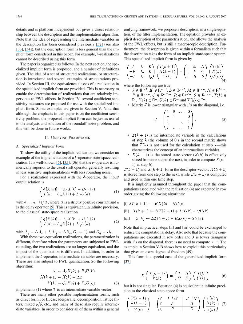
unifying framework, we propose a description, in a single equa-tion, of the filter implementation. The equation provides an ex-plicit description of the parametrization, and allows the analysisof the FWL effects, but is still a macroscopic description. Fur-thermore, the description is given within a formalism such thatthe description takes the form of an implicit state-space system.This specialized implicit form is given by

(4)where the following are true.

• , , , , ,, , , ,

, , and .• Matrix is lower triangular with 1’s on the diagonal, i.e.

.... . .

...(5)

• is the intermediate variable in the calculationsof step (the column of 0’s in the second matrix showsthat is not used for the calculation at step —thischaracterizes the concept of an intermediate variable).

• is the stored state-vector ( is effectivelystored from one step to the next, in order to compute

at step ).and form the descriptor-vector:

is stored from one step to the next, while is computedand used within one time step.

It is implicitly assumed throughout the paper that the com-putations associated with the realization (4) are executed in roworder giving the following algorithm:

[i]

[ii]

[iii]

Note that in practice, steps [ii] and [iii] could be exchanged toreduce the computational delay. Also note that because the com-putations are executed in row order and is lower triangularwith 1’s on the diagonal, there is no need to compute . Theexample in Section V-B shows how to exploit this particularitythat gives an extra degree of freedom (49).

This form is a special case of the generalized implicit form[37]

(6)

but it is not singular. Equation (4) is equivalent in infinite preci-sion to the classical state-space form

(7)

HILAIRE et al.: UNIFYING FRAMEWORK FOR FWL REALIZATIONS 1767

with , , and where

(8)

(9)

Note that (7) corresponds to a different parametrization than (4).The system transfer function is given by

(10)

B. Definitions

To complete the framework, the following definitions are re-quired.

Definition 1: A realization, , is defined by the specific setof matrices , , , , , , , , and used to describe arealization with the implicit form of (4):

(11)

Remark 1: can also be defined by the matrix

(12)

and the dimensions , , and , so could be defined by.

Definition 2: denotes the set of realizations with transferfunction . These realizations are said to be equivalent.

In order to encompass realizations with some special struc-ture ( -operator state-space, -operator state-space, direct form,cascade, lattice filters, etc.), we define a set of realizations thatpossess a particular structure.

Definition 3: A structuration1 is a set of realizationshaving a common structure: some coefficients or some dimen-sions are fixed a priori.

Some examples of common structurations are given in thenext section.

Definition 4: is the set of equivalent structured realiza-tions. Realizations from are structured according to and

have a transfer function . Hence, .Definition 5: A parametrization of a realization is the set

of coefficients of that are significant for the realization.For example, with the -operator state-space realization of

(2), the parametrization is given by the matrices , ,and . But for the -operator state-space realization of (1), theparametrization is given by the matrices , , , and theparameter . We will see in the next section that the -operatorstate-space realization includes some additional parameters thatare always set to unity or zero. These are not ‘significant coef-ficients’ and hence are not included in the parametrization.

1This is a useful French word that we have purloined. It is also used in thefield of social sciences. Here it means the set of structured realizations.

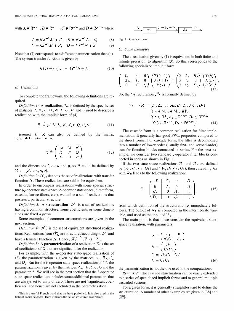
Fig. 1. Cascade form.

C. Some Examples

The -realization given by (1) is equivalent, in both finite andinfinite precision, to algorithm (3). So this corresponds to thefollowing specialized implicit form:

(13)So, the -structuration is formally defined by

(14)

The cascade form is a common realization for filter imple-mentation. It generally has good FWL properties compared tothe direct forms. For cascade form, the filter is decomposedinto a number of lower order (usually first- and second-order)transfer function blocks connected in series. For the next ex-ample, we consider two standard -operator filter blocks con-nected in series as shown in Fig. 1.

If the two state-space realizations and are definedby and , then cascadingwith leads to the following realization:

(15)

from which definition of the structuration immediately fol-lows. The output of is computed in the intermediate vari-able, and used as the input of .

The main point is that if we consider the equivalent state-space realization, with parameters

(16)

the parametrization is not the one used in the computations.Remark 2: The cascade structuration can be easily extended

to a series of specialized implicit forms and to general multiplecascaded systems.

For a given form, it is generally straightforward to define thestructuration. A number of other examples are given in [38] and[39].

1768 IEEE TRANSACTIONS ON CIRCUITS AND SYSTEMS—I: REGULAR PAPERS, VOL. 54, NO. 8, AUGUST 2007

III. EQUIVALENT CLASSES

In order to exploit the potential offered by the specializedimplicit form in improving implementations, it is necessary, todescribe sets of equivalent system realizations. However, non-minimal realizations may provide better implementations (the-form can be seen as a nonminimal realization when expressed

in the implicit state-space form with the shift operator. Hence,the notion of equivalence needs to be extended so that the systemstate dimension does not need to be preserved. The InclusionPrinciple, introduced by Siljak and Ikeda [40], [41] in the con-text of decentralized control, is useful here as it allows the for-malization of the equivalence and inclusion relations betweentwo system realizations.

Definition 6: Consider two systems and , with state di-mension and respectively, described in classical state-space form by matrices , , ,

, and . System is said tobe included in system (denoted by ) if there exists

such that and, for any initialstate of and any input , the choice ofthe initial state of implies

(17)

Remark 3: Equation (17) implies that system contains allthe necessary information to describe the behavior of .

The principle is extended here to the specialized implicit formin order to characterize equivalence classes. An equivalenceclass is defined by a certain minimal realization and all the re-alizations that include this realization. They can be built usingthe following proposition:

Proposition 1: Consider a realizationwith dimensions .

A realization that includes can be constructed as follows.• Choose and such that .• Choose such that ,

such that andsuch that .

• Choose complementary matrices2 ,

, , , ,, , and

such that, if we denote ,, , ,

, , ,, and,

then , ,,

and are satisfied.

2These matrices are called complementary matrices.M is complementaryin that it fills the gap between ~X and the similarity onX : ~X = T XT +M .

If so, the realization in-cludes the realization .

Proof: The proof can be derived directly from the charac-terization of the Inclusion Principle [40], [42], [43]. The detailsare omitted here but can be found in [38].

Although this proposition gives the formal description ofequivalent classes, it is of practical interest to consider real-izations of the same dimensions ( and ) wheretransformations from one realization to another is only a simi-larity transformation.

Proposition 2: Consider a realization .All the realizations with

(18)

and , , are nonsingular matrices, are equivalent to .It is also possible to just consider a subset of similarity trans-

formations that preserve a particular structure, say cascade ordelta. For example, if an initial -structured realization

is given, the subset of equivalent -structuredrealization is defined by

nonsingular(19)

In addition to a description of the various existing realizationswith the exact parametrization, this formalism gives an algebraiccharacterization of equivalent classes. These classes can be usedto search for an optimal structured realization (see Section V-A).

IV. SENSITIVITY MEASURES

In order to be able to accurately assess the suitability of a par-ticular realization in the specialized implicit form, some mea-sure of the coefficient sensitivity are required. The measuresneed to be computationally tractable but also need to accountfor the fact that common structured realizations (e.g., ) containmany coefficients that are either zero or unity and hence do notcontribute to the FWL effects. Such coefficients are known astrivial parameters. Furthermore, it is useful if the measures cantake into account the choice of arithmetic format (floating pointor fixed point) of the coefficients’ representation.

A. Coefficient Quantization

A coefficient’s quantization depends both on their value andtheir representation.

Firstly if the value of a coefficient is such that it will bequantized without error, then that parameter makes no contribu-tion to the overall coefficient sensitivity. Hence, we introduceweighting matrices to (and also ) respectively as-sociated with matrices to of a realization, such that

if is exactly implementedotherwise.

(20)

HILAIRE et al.: UNIFYING FRAMEWORK FOR FWL REALIZATIONS 1769

Secondly, different representation schemes may be considered.Here, we consider both fixed-point and floating-point represen-tations of coefficients expressed using bits.

A fixed-point coefficient is represented by ,where , is an integer coded with bits and aninteger (not stored in the representation) such that

. The quantized of is such that .A floating-point coefficient is represented by

where (or for a normalized floating-pointrepresentation) and is an integer coded with bits3

. The quantized of is, in thiscase, such that .

The choice of and can be unique for each coefficient( and , where isthe ceiling operator). Alternatively, and are defined for agroup of coefficients (in order to reduce the required bit-shiftsand the subsequent computational cost). This defines the block-fixed-point and block-floating-point schemes. Following [44],we introduce the generalized dynamic range bit (or ) and the precision bit length ( or ).

Usually, the blocks used in block-representation correspondto the matrices to , but there is no necessity for this, andblocks can be chosen at will. To define the blocks of a realization

, we introduce the matrix such that

the largest absolute value ofthe block in which resides (21)

This allows a completely general definition of the blocks.Thus, there could be just a single unique block, or every blockcould consist of only one coefficient. For example, denoting

as a matrix of 1’s and

(22)

then using a block-representation corresponding to the matricesto gives

With a single unique block for we get, and for one block per coeffi-

cient we get .Proposition 3: During the quantization process, is per-

turbed to where

for fixed-point representationfor floating-point representation

(23)

is a matrix dependant on the precision bit length, anddenotes the Schur product. If is the precision bit-length of

, then .Remark 4: With this formalism for the different representa-

tion schemes, note that the choice of the scale parameter ( or) is defined for each coefficient ( and

3The difference with fixed-point is that e is coded with � bits and can bechanged. With fixed-point, � is fixed and implicit.

) and that it is also possible to de-fine the minimum bit length to code each coefficient withoutoverflow or underflow [38].

B. Transfer Function Sensitivity Measure

The sensitivity measure proposed here extends the measureproposed by Gevers and Li [5] to the specialized implicit state-space form as well as accounting for trivial parameters and thecoefficient representation.

Let denote the transfer function per-turbed by the quantization process. Then, in the single-inputsingle-output (SISO) case, :

(24)

Then

(25)

where is the -norm. It is easy to see that

(26)

and so (25) leads to the following transfer function sensitivitymeasure:

Definition 7 (SISO Transfer Function Sensitivity): Considera realization with an associated matrix .The sensitivity of the realization’s transfer function with re-spect to all the nontrivial coefficients of , is defined in theSISO case by

(27)

Remark 5: The measure differs from the measure pro-posed by Gevers and Li [5] for SISO classical state-space fixed-point realizations which is defined by

(28)

For the definition of , the term is ignoredbecause it is invariant to the possible realization. However, forthe specialized implicit form, and so the sen-sitivity of the direct feed-through term, , is dependenton the realization.

This measure can be extended to the multiple-input multipleoutput (MIMO) case. However it is also useful to be able to con-sider the contribution of each coefficient to the overall sensi-tivity. The transfer function sensitivity matrix, denoted by ,is the matrix of the -norm of the sensitivity of the transferfunction with respect to each coefficient . It is defined by

(29)

1770 IEEE TRANSACTIONS ON CIRCUITS AND SYSTEMS—I: REGULAR PAPERS, VOL. 54, NO. 8, AUGUST 2007

and allows the evaluation of the overall impact of each coeffi-cient. It can be used to evaluate the overall sensitivity. From theproperties of the -norm, we have

(30)

where is the Frobenius norm.Definition 8: The MIMO transfer function sensitivity is de-

fined by

(31)

Next, we introduce a new operator that simplifies the subse-quent expressions for and the transfer function sensitivitymatrix.

Definition 9: The operator is defined by

(32)

where and and where is theclassical operator that transforms a matrix to a column vector.So .

Lemma 1: Consider two matrices (or transfer functions),and , that are assumed to be independent of a

matrix . Then

(33)

and

(34)

Proof: The proof can be found in [38] and comes from

(35)

Proposition 4:

(36)

where

and the dimensions of the transfer functions to are ,, and respectively.

Proof: From the application of Lemma 1 with (8) and (9)to (10). Details are given in [38].

Proposition 5: Consider a matrix and three transfer func-tion matrices , and of appropriate dimensions such that

(37)

The sensitivity matrix is given by

(38)

Proof: The proof is straightforward and can be found in[38].

C. Pole Sensitivity Measure

The transfer function sensitivity does not explicitly con-sider the stability of the system. To ensure that the imple-mentation is stable, the sensitivity of the poles needs to beconsidered. Let denote the poles of a realization

. These poles are perturbed during thequantization process to with

(39)

Clearly, this expression provides a means by which the min-imum bit-length to preserve stability can be determined a priori.This is explored in [38] and [45].

We can define the following pole sensitivity measure.Definition 10: Consider a realization

and associated quantization description matrix . The pole sen-sitivity measure of is defined by

(40)

The following lemma is required prior to providing a meansof evaluating .

Lemma 2: ([28]) Consider a differentiable function, and two matrices and .

Let , and be constant matrices with appropriatedimensions, then the following results hold.

• If , then

• If , then

Proposition 6:

(41)

Proof: Apply Lemma 2 to (8).The term can be evaluated using the following

lemma.Lemma 3: Let be diagonalisable. Let

be its eigenvalues, and the corre-

sponding right eigenvectors. Denote and

. Then

(42)

HILAIRE et al.: UNIFYING FRAMEWORK FOR FWL REALIZATIONS 1771

and

(43)

where denotes the conjugate operation, the real part andthe transpose conjugate operator.

Proof: The procedure for the proof can be found in [30].Remark 6: In a similar manner to the transfer function sensi-

tivity matrix, (29), a pole sensitivity matrix can be constructedto evaluate the overall impact of each coefficient. Let de-note the pole sensitivity matrix defined by

(44)

The pole sensitivity measure is then given by

(45)

V. ILLUSTRATIVE EXAMPLE

A. Optimal Realization Problem

The problem of determining the best realization can be posedas follows:

Problem 1 (Optimal Realization Problem): Consider atransfer function and a sensitivity measure . The optimaldesign problem is to find the best realization with transferfunction according to the criteria , that is

(46)

Due to the size of , this problem cannot be solved prac-tically. Indeed, a solution may even have infinite dimension.Hence, the following problem is introduced to restrict the searchto a particular structuration.

Problem 2 (Optimal Structured Realization Problem): Theproblem to find the optimal structured realization , that is

(47)

The Inclusion Principle (Propositions 1 and 2) providesthe means to search over the structured realizations set .Since the measure could be nonsmooth and/or nonconvex,the Adaptive Simulated Annealing (ASA) [46] method hasbeen chosen to solve Problem 2. This method has workedwell for other optimal realization problems [30]. The resultingoptimal sensitivities for the measures proposed in Section IVare presented next.

B. Example

To illustrate the use of the proposed measures and the optimaldesign problem, we consider a sixth-order narrowband low-passfilter from [27] given by

TABLE IMEASURES FOR DIFFERENT REALIZATIONS

. The poles are,

and (all the computations areperformed with double floating-point precision, but the resultsare quoted only to 4 significant digits). The weighting matrix

is constructed according to (20) (only 0, 1 are consideredas exactly implemented). Note that the optimizations are per-formed using the pole sensitivity measure , but could also bedone using the transfer function sensitivity measure or a mixedmeasure.

The following realizations are considered.

Direct form II with shift-operator : it correspondsto a canonical state-space form: the transfer functioncoefficients directly appear in .

Balanced classical state-space realization.

-optimal classical state-space realization: the set ofequivalent classical state-space realizations is searchedusing (48), shown at the bottom of the next page, where

is one classical state-space realizationof and is a nonsingular matrix.

-optimal implicit state-space realization: we considerall the equivalent realizations described by (49), shownat the bottom of the next page, where is a lowertriangular matrix [as for in (5)]. This can be describedin the implicit state-space framework by (50), shown atthe bottom of the next page, and equivalent realizationscan be searched with the similarity shown in (51) atthe bottom of the next page, where is a nonsingularmatrix and is chosen so that is still lowertriangular (in practice, the coefficients of the new matrix

are chosen by the optimization algorithm, and isthen deduced).

-optimal state-space -realization : the-structured equivalent set [see (19)] is searched,

with an initial realization given as for (13).

The values of the sensitivity measures for the various realiza-tions are given in Table I. Note that the balanced realizationhas the best transfer function sensitivity. This is not surprisingsince it is known that balanced realizations are optimal in an-other transfer function sensitivity sense [5]. The pole sensitivityof is fairly good, but is not minimal and can be reduced by afactor of 4 by using the state-space realization. However, real-izations , and have a poor transfer function sensitivity.

1772 IEEE TRANSACTIONS ON CIRCUITS AND SYSTEMS—I: REGULAR PAPERS, VOL. 54, NO. 8, AUGUST 2007

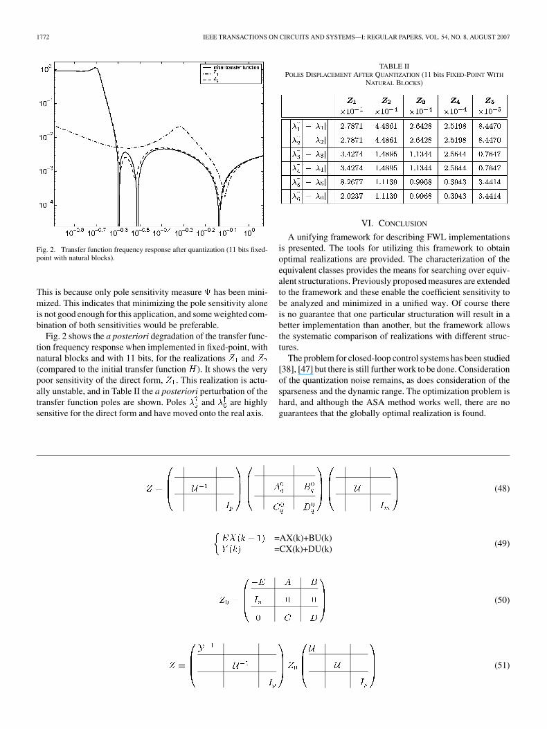
Fig. 2. Transfer function frequency response after quantization (11 bits fixed-point with natural blocks).

This is because only pole sensitivity measure has been mini-mized. This indicates that minimizing the pole sensitivity aloneis not good enough for this application, and some weighted com-bination of both sensitivities would be preferable.

Fig. 2 shows the a posteriori degradation of the transfer func-tion frequency response when implemented in fixed-point, withnatural blocks and with 11 bits, for the realizations and(compared to the initial transfer function ). It shows the verypoor sensitivity of the direct form, . This realization is actu-ally unstable, and in Table II the a posteriori perturbation of thetransfer function poles are shown. Poles and are highlysensitive for the direct form and have moved onto the real axis.

TABLE IIPOLES DISPLACEMENT AFTER QUANTIZATION (11 bits FIXED-POINT WITH

NATURAL BLOCKS)

VI. CONCLUSION

A unifying framework for describing FWL implementationsis presented. The tools for utilizing this framework to obtainoptimal realizations are provided. The characterization of theequivalent classes provides the means for searching over equiv-alent structurations. Previously proposed measures are extendedto the framework and these enable the coefficient sensitivity tobe analyzed and minimized in a unified way. Of course thereis no guarantee that one particular structuration will result in abetter implementation than another, but the framework allowsthe systematic comparison of realizations with different struc-tures.

The problem for closed-loop control systems has been studied[38], [47] but there is still further work to be done. Considerationof the quantization noise remains, as does consideration of thesparseness and the dynamic range. The optimization problem ishard, and although the ASA method works well, there are noguarantees that the globally optimal realization is found.

(48)

=AX(k)+BU(k)=CX(k)+DU(k)

(49)

(50)

(51)

HILAIRE et al.: UNIFYING FRAMEWORK FOR FWL REALIZATIONS 1773

REFERENCES

[1] J. E. Bertram, “The effects of quantization in sampled-feedback sys-tems,” Trans. Amer. Inst. Elect. Eng., vol. 77, pp. 177–182, 1958.

[2] J. B. Slaughter, “Quantization errors in digital control systems,” IEEETrans. Autom. Contr., vol. AC-9, no. 1, pp. 70–74, Jan. 1964.

[3] B. Liu, “Effects of finite word-length on the accuracy of digitalfilters—A review,” IEEE Trans. Circuit Theory, vol. 18, no. 6, pp.670–677, Jun. 1971.

[4] D. Williamson, Digital Control and Implementation, Finite WordlengthConsiderations. London, U.K.: Prentice-Hall, 1992.

[5] M. Gevers and G. Li, Parametrizations in Control, Estimation and Fil-tering Probems. London, U.K.: Springer-Verlag, 1993.

[6] R. S. H. Istepanian and J. F. Whidborne, “Finite-precision computingfor digital control systems: Current status and future paradigms,” inDigital Controller Implementation and Fragility: A Modern Perspec-tive, R. S. H. Istepanian and J. F. Whidborne, Eds. London, U.K.:Springer-Verlag, 2001, ch. 1, pp. 1–12.

[7] I. W. Sandberg, “Floating-point-roundoff accumulation in digital-filterrealizations,” Bell Syst. Tech. J., vol. 46, no. 8, pp. 1775–1791,1967.

[8] C. Mullis and R. Roberts, “Synthesis of minimum roundoff noise fixedpoint digital filters,” IEEE Trans. Circuits Syst., vol. CAS-23, no. 9, pp.551–562, Sep. 1976.

[9] S. Y. Hwang, “Minimum uncorrelated unit noise in state-space digitalfiltering,” IEEE Trans. Acoust., Speech, Signal Process., vol. ASSP-25,no. 4, pp. 273–281, Aug. 1977.

[10] J. Knowles and E. Olcayto, “Coefficient accuracy and digital filter re-sponse,” IEEE Trans. Circuits Syst., vol. CAS-15, no. 1, pp. 31–41,Mar. 1968.

[11] R. C. Agarwal and C. S. Burrus, “New recursive digital filter structureshaving very low sensitivity and roundoff noise,” IEEE Trans. CircuitsSyst., vol. CAS-22, no. 12, pp. 921–927, Dec. 1975.

[12] V. Tavsanoglu and L. Thiele, “Optimal design of state-space digitalfilters by simultaneous minimization of sensibility and roundoff noise,”IEEE Trans. Acoust., Speech, Signal, Process., vol. CAS-31, no. 10, pp.884–888, Oct. 1984.

[13] L. Thiele, “Design of sensitivity and roundoff noise optimal state-spacediscrete systems,” Int. J. Circuit Theory Appl., vol. 12, pp. 39–46,1984.

[14] L. Thiele, “On the sensitivity of linear state space systems,” IEEETrans. Circuits Syst., vol. CAS-33, no. 5, pp. 502–510, 1986.

[15] W.-Y. Yan and J. B. Moore, “On L -sensitivity minimization of linearstate-space systems,” IEEE Trans. Circuits Syst., Fundam. TheoryAppl., vol. 39, no. 8, pp. 641–648, Aug. 1992.

[16] G. Li, B. D. O. Anderson, M. Gevers, and J. E. Perkins, “Optimal FWLdesign of state space digital systems with weighted sensitivity mini-mization and sparseness consideration,” IEEE Trans. Circuits Syst. II,Exp. Briefs, vol. 39, no. 5, pp. 365–377, May 1992.

[17] C. Xiao, “Improved L -sensitivity for state-space digital system,”IEEE Trans. Signal Process., vol. 45, no. 4, pp. 837–840, Apr. 1997.

[18] T. Hinamoto, S. Yokoyama, T. Inoue, W. Zeng, and W. Lu, “Analysisand minimization of L -sensitivity for linear systems and two-dimen-sional state-space filters using general controllability and observabilitygramians,” IEEE Trans. Circuits Syst., Fundam. Theory Appl., vol. 49,no. 9, pp. 1279–1289, Sep. 2002.

[19] M. Iwatsuki, M. Kawamata, and T. Higuchi, “Statistical sensitivity andminimum sensitivity structures with fewer coefficients in discrete timelinear systems,” IEEE Trans. Circuits Syst., vol. 37, no. 1, pp. 72–80,Jan. 1989.

[20] W. J. Lutz and S. L. Hakimi, “Design of multi-input multi-output sys-tems with minimum sensitivity,” IEEE Trans. Circuits Syst., vol. 35,no. 9, pp. 1114–1122, Sep. 1988.

[21] A. G. Madievski, B. D. O. Anderson, and M. Gevers, “Optimum re-alizations of sampled-data controllers for FWL sensitivity minimiza-tion,” Automatica, vol. 31, no. 3, pp. 367–379, 1995.

[22] W.-S. Lu and T. Hinamoto, “Jointly optimized error-feedback andrealization for roundoff noise minimization in state-space digitalfilters,” IEEE Trans. Signal Process., vol. 53, no. 6, pp. 2135–2145,Jun. 2005.

[23] T. Hinamoto, H. Ohnishi, and W.-S. Lu, “Minimization of L sensi-tivity for state-space digital filters subject toL -dynamic-range scalingconstraints,” IEEE Trans. Circuits Syst. II, Exp. Briefs, vol. 52, no. 10,pp. 641–645, 2005.

[24] J. F. Kaiser, “Digital filters,” in System Analysis by Digital Computer,F. F. Kuo and J. F. Kaiser, Eds. New York: Wiley, 1966, pp.218–285.

[25] P. E. Mantey, “Eigenvalue sensitivity and state-variable selection,”IEEE Trans. Autom. Contr., vol. AC-13, no. 3, pp. 263–269, Mar.1968.

[26] R. Skelton and D. Wagie, “Minimal root sensitivity in linear systems,”J. Guidance, Contr. Dyn., vol. 7, no. 5, pp. 570–574, 1984.

[27] D. Williamson, “Roundoff noise minimization and pole–zero sensi-tivity in fixed-point digital filters using residue feedback,” IEEE Trans.Acoust., Speech, Signal Process., vol. ASSP-34, no. 5, pp. 1210–1220,Oct. 1986.

[28] G. Li, “On the structure of digital controllers with finite word lengthconsideration,” IEEE Trans. Autom. Contr., vol. 43, no. 5, pp. 689–693,May 1998.

[29] J. F. Whidborne, R. Istepanian, and J. Wu, “Reduction of controllerfragility by pole sensitivity minimization,” IEEE Trans. Autom. Contr.,vol. 46, no. 2, pp. 320–325, Feb. 2001.

[30] J. Wu, S. Chen, G. Li, R. Istepanian, and J. Chu, “An improved closed-loop stability related measure for finite-precision digital controller re-alizations,” IEEE Trans. Autom. Contr., vol. 46, no. 7, pp. 1162–1166,Jul. 2001.

[31] H.-J. Ko and W. S. Yu, “Guaranteed robust stability of the closed-loopsystems for digital controller implementations via orthogonal hermi-tian transform,” IEEE Trans. Syst., Man, Cybern., vol. 34, no. 4, pp.1923–1932, Aug. 2004.

[32] D. S. K. Chan, “The structure of recursible multidimensional discretesystems,” IEEE Trans. Autom. Contr., vol. AC-25, no. 4, pp. 663–673,Aug. 1980.

[33] D. S. K. Chan, “Constrained minimization of roundoff noise infixed-point digital filters,” in Proc. IEEE Int. Conf. Acoust., Speech,Signal Process. (ICASSP ’79), Washington, DC, Apr. 1979, pp.335–339.

[34] P. Moroney, A. S. Willsky, and P. K. Houpt, “The digital implementa-tion of control compensators: The coefficient wordlength issue,” IEEETrans. Autom. Contr., vol. AC-25, no. AC-4, pp. 621–630, Aug. 1980.

[35] R. Middleton and G. Goodwin, Digital Control and Estimation, a Uni-fied Approach. Englewood Cliffs, NJ: Prentice-Hall, 1990.

[36] R. Goodall, “Perspectives on processing for real-time control,” Ann.Rev. Contr., vol. 25, pp. 123–131, 2001.

[37] J. Aplevich, Implicit Linear Systems. New York: Springer-Verlag,1991.

[38] T. Hilaire, “Analyse et synthèse de l’implémentation de lois de contrôle-commande en précision finie (étude dans le cadre des applicationsautomobiles sur calculateur embarquée),” Ph.D. dissertation, Dept.Comp. Sci., Université de Nantes, Nantes, France, Jun. 2006.

[39] T. Hilaire, P. Chevrel, and Y. Trinquet, “Implicit state-space repre-sentation: A unifying framework for FWL implementation of LTI sys-tems,” in Proc. 16th IFAC World Congr., Jul. 2005, CDROM.

[40] M. Ikeda, D. Siljak, and D. White, “An inclusion principle for dynamicsystems,” IEEE Trans. Autom. Contr., vol. 29, no. AC-3, pp. 244–249,Mar. 1984.

[41] D. Siljak, Decentralized Control of Complex Systems. New York:Academic, 1991.

[42] M. Ikeda and D. Siljak, “Overlapping decompositions, expansions, andcontractions of dynamic systems,” Large Scale Syst., vol. 1, pp. 29–38,1980.

[43] L. Bakule, J. Rodellar, and J. Rossell, “Structure of expansion-contrac-tion matrices in the inclusion principle for dynamic systems,” SIAMMatrix Anal. Appl., vol. 21, no. 4, pp. 1136–1155, 2000.

[44] J. Wu, S. Chen, and J. Chu, “Comparative study on finite-precisioncontroller realizations in different representation schemes,” in Proc. 9thAnnual Conf. Chinese Autom. Comput. Soc., Luton, U.K., Sep. 2003,pp. 257–262.

[45] J. Wu, S. Chen, J. F. Whidborne, and J. Chu, “A unified closed-loopstability measure for finite-precision digital controller realizations im-plemented in different representation schemes,” IEEE Trans. Autom.Contr., vol. 48, no. 5, pp. 816–823, May 2003.

[46] L. Ingber, “Adaptive simulated annealing (ASA): Lessons learned,”Contr. Cybern., vol. 25, no. 1, pp. 33–54, 1996.

[47] T. Hilaire, P. Chevrel, and J. Whidborne, “Low parametric closed-loopsensitivity realizations using fixed-point and floating-point arithmetic,”in Proc. Eur. Contr. Conf. (ECC’07), Kos, Greece, Jul. 2–5, 2007, tobe published.

1774 IEEE TRANSACTIONS ON CIRCUITS AND SYSTEMS—I: REGULAR PAPERS, VOL. 54, NO. 8, AUGUST 2007

Thibault Hilaire received the M.Sc. and Ph.D. de-grees in control and applied computing sciences fromUniversity of Nantes, Nantes, France, in 2003 and2006, respectively.

He is currently a Postdoctoral Researcher atthe IRISA Laboratory (R2D2), Institut Nationalde Recherche en Informatique et en Automatique(INRIA), Lannion, France. He is working on finiteword length implementation (sensitivity measures,roundoff noise, optimal design, etc.).

Philippe Chevrel received the Ph.D. degree from theUniversity of Paris XI, in 1993.

He is currently a Professor at Ecole des Mines deNantes, Nantes, France, and is a member of the con-trol team at Institut de Recherche en Communica-tions et Cybernétique de Nantes (IRCCyN), NantesFrance. He is author or coauthor of nearly 100 re-search publications and reports, including patents andbook chapters. His research interests include robustcontrol, structured control and control implementa-tion, from theoretical to practical, with applications

to automotive systems, power systems, and vibration control.

James F. Whidborne (M’96) received the B.A.degree in engineering from Cambridge University,Cambridge, U.K., in 1982, and the M.Sc. andPh.D. degree in systems and control from UMIST,Manchester, U.K., in 1987 and 1992, respectively.

He is currently a Senior Lecturer in the Departmentof Aerospace Sciences, Cranfield University, Cran-field, U.K. He has over 100 research publications, in-cluding three books and his research interests includeoptimal finite-precision controller implementations,multi-objective robust control design, fluid flow con-

trol and control of unmanned air vehicles.