1

A Variable Risk Propensity Model of Technological Risk Taking

Lee Fleming Morgan T97

Harvard Business School Boston, MA 02163 lfleming@hbs.edu

(617) 495-6613

Philip Bromiley Department of Strategic Management

Carlson School of Management University of Minnesota 321 19th Avenue South

Minneapolis, MN 55455 pbromiley@csom.umn.edu

(612) 624-5746

Dec. 3, 2000 We would like to thank Laurie Calhoun for her editing assistance, Sarah Woolverton, Ching Han Wong, and Evelina Fedorenko for their help in collecting Compustat and Patent data, and the Carlson School of Management and the Harvard Business School Division of Research for their support.

2

Abstract

Patent data have recently become widely available and easily manipulated. Many studies

have established a correlation between a patent’s quality or value and future prior art

citations to that patent. Recent work in negative binomial count models has also

provided a method to estimate effects on the mean as well as the variance of prior art

citations. We exploit this opportunity of new data and methods by proposing and testing

a model of technological risk taking, as a function of a firm’s available resources and risk

propensity. We measure resources as a firm’s R&D spending and per the behavioral

literature on risk taking, risk propensity as distance from a firm’s industry’s return on

assets. We find strong support for the predictions of mean citation counts, and mostly

insignificant and contrary evidence for the predictions of the dispersion of citation

counts. The work provides evidence for behavioral influences on decision making and a

promising method for future investigation of influences upon the quality and variability

of invention.

3

Introduction

The availability of large patent databases has been widely exploited in the study of

invention and innovation. For example, early work examined the influence of R&D

expenditures (Hausman, Hall, and Griliches 1984) and size (Henderson and Cockburn

1996) on a firm's technological success as measured by its patent count. Basic counts do

not control for patent quality, however. Recent work partially addresses this weakness by

using the number of prior art citations from future patents to measure a patent’s quality. 1

Researchers have used prior art citations to evaluate the basicness of university versus

private firm invention (Trajtenberg, Henderson, and Jaffe 1997) and to argue that

organizational aging increases the rate but not the quality of inventive processes, as

measured by an increase in the rate of patenting but a decrease in the citation rate to those

patents (Sorenson and Stuart 2000).

Econometric techniques have also recently advanced for handling the idiosyncrasies of

these data. Early work developed negative binomial models that estimated the influences

of research and development investment on the number of patents granted to a firm

(Hausman, Hall, and Griliches 1984, Cameron and Trivedi 1986). Recent techniques

allow for the estimation of effects on the variance of negative binomial data as well (King

1989, Jorgenson 1997). Given that prior art citations are also distributed as negative

binomial, these data and models enable estimation of inventive quality and variance in

1 The U.S. Patent Office requires that each applicant demonstrate an awareness of prior art in the field, in order that s/he can establish the novelty of the application, relative to previous technology. The patent examiner can supplement the applicant’s list of citations to previous patents. All the published research that we are aware of (Trajtenberg 1990, Albert et. al. 1991, Scherer and Harhoff 2000, Hall, Jaffe, and Trajtenberg 2000) has demonstrated a positive correlation between the social, technological, and economic value of a patent and the number of future prior art citations to the patent.

4

quality. While this has been done for qualitatively argued hypotheses (Fleming

forthcoming), we propose a formal model that predicts the mean and dispersion of patent

citations as a function of firm risk propensity and resources. We draw on the behavioral

literature on risk taking and aspiration points for theoretical motivation and measures of

risk propensity.

The Model

We frame the substantive problem simply: management needs to allocate resources

across four kinds of research and development (R&D) projects. It allocates money at

time one and receives all returns at time two, shortly after time one. Among other things,

the model predicts the expected quality of the firm’s inventions (i.e., how many citations

the firm’s patents receive) and the variance of that expected quality.

For modeling purposes, assume that a firm has one assured investment and three

innovation projects available. The assured investment provides a certain (i.e., risk-free)

but relatively low return. In this investment, additional funds provide additional returns

much as they do in a bank account. The other three categories represent research projects

of low, medium, and high levels of risk. Additional funds invested in these categories

change the probability of success but not the returns if the project succeeds. The firm

invests all of its resources across the four kinds of projects (we will refer to the four

opportunities as projects, even though the financial investment is neither risky nor a

technology project).

5

Each project has a probability of success conditional on investing one unit of resources in

it. Each unit of resources the firm invests in a project gives the firm an independent draw

on a Bernoulli distribution that has the outcomes of project success or failure. The

project succeeds if any of the draws comes up a success. Consequently, the probability

of a project succeeding increases with additional resources (i.e., draws) but at a

decreasing rate (i.e., if the probability of success on the first draw is 50%, investing two

units only increases the probability of success to 75%). This provides an underlying

causal mechanism consistent with other work that assumes marginally decreasing returns

to research investment (see, for instance, Cohen and Klepper 1996).

The firm needs a decision rule to allocate resources across the four projects. We use a

simple utility function that allows firms to have different risk preferences. The firm

optimizes expected utility from the four investment projects. The allocation varies

depending on two parameters: (i) risk propensity, reflected in the curvature of the utility

function and (ii) resources available. Both of these parameters vary across firms. The

analysis of the model examines how varying these two factors (risk propensity and

resources) influences the allocation of funds across projects. We assume the probability

of an investment’s success is independent from the probabilities of the other investments’

successes, given the resources invested. The portfolio can have a range of outcomes from

all projects succeeding to no projects succeeding with all permutations in between.

We motivate the model of risk taking from the arguments of several research streams.

Many of these streams propose that firms exhibit varying risk preferences. For example,

6

agency theorists ascribe firm level risk aversion to managers operating under governance

and incentive systems that do not fully compensate for the individuals' risk aversion

(Jensen and Meckling, 1976). Behavioral models of the firm generally assume that firms

avoid uncertainty (Cyert and March 1992; March and Shapira 1992). Some firms may

seek risk, however. Excessive or incorrect application of agency theorists’ prescriptions

could create managerial risk seeking. Alternatively, certain firm conditions (e.g.,

expected bankruptcy or unexpected attainment of performance goals) may result in risk

seeking. Firms’ managers may also be over confident in their control and predictive

abilities (Kahneman and Lovallo 1993).

Since all investments are in the gain realm in our model, we will use the empirically

derived utility function from Tversky and Kahneman (1992) where U is utility, X is the

outcome value, and b is the risk parameter (equation 1).

bxU(x) = (1)

The firm maximizes its expected utility – the utility of each of its portfolio outcomes

times the likelihood of that outcome (equation 2). Maximizing equation 2 equates to

maximizing expected value when the risk parameter equals one.

boutcome)portfoliopayoffo*(portfolioutcome)(portfolioUtilityFirmoutcomes

portfolioall∑=

Pr (2)

7

To implement equation (2), the model needs the probability of portfolio outcomes and the

portfolio payoffs. As described above, the model has one safe investment and three risky

investments. The allocation of resources (Ri) to the safe investment returns Ri times the

allocated investment plus some return that we set exogenously. This investment acts as a

corporate hurdle rate; the firm puts funds into the safe investment if current projects do

not merit funding.

All three risky projects provide a fixed return if successful. The probability of success of

any particular project increases with greater resource allocation, but at a decreasing rate.

Assuming binomial trials, the probability of success for a project, given the allocation of

Ri units of resources, is one minus the probability of Ri trials coming out failures

(equation 3).

iRi ent in i)of investm one unit (success |)Rroject i |(success p ]Pr1[1Pr −−= (3)

To evaluate the returns on the full portfolio, the model calculates the probability and

payoffs for all possible combination outcomes of the four projects (i.e., success or failure

on each project). With one safe and three risky investments, the model has 24=16

possible portfolio outcomes. For example, one portfolio outcome is that all four projects

succeed and another portfolio outcome is that project four succeeds and projects one,

two, and three fail. Each project i has two possible outcomes (Oi =success or failure).

Conditional on the resources applied to the project, each project has a probability of

success P(Oi = success|Ri). Given the assumption of independence between projects, the

8

probability of a given portfolio outcome is the product of the probabilities for each of the

four project outcomes (equation 4).

)|Rme O has Outco(project i ) ,O,O,O outcome O(portfolio,,,i

i projects ii∏

=

=4321

4321 PrPr

(4)

The payoff for each portfolio outcome equals the sum of the payoffs from the successful

projects in the portfolio (equation 5).

i)or project*(payoff f)( ,O,O,OO | outcome payoffPortfolio ,,,i

i projectsssfuli is succe project∑

=

=4321

4321 1

(5)

To determine the expected utility of the portfolio, the model allocates resources across

projects to maximize the expected utility calculated as:

∑= outcomes

lioall portfo

b),O,O,O Oio payoff|)*(portfol,O,O,O(OtyFirm Utili 43214321Pr

(6)

9

Model Parameters

The model requires a number of parameters: the probabilities and returns for projects,

risk propensity, and resources. Let us consider each in turn.

For simplicity, we set the expected return from allocating the first unit of resources to any

innovation equal across innovations, i.e., for all three risky projects, the expected value

for the first unit of resources (the probability of success times the payoff) is constant

across investments. Thus, low risk projects have low returns and high-risk projects have

high returns. This reflects the typical situation where incremental and easy innovations

generate assured but small returns (high probability of success but low returns if

successful). Breakthrough and difficult innovations generate big returns - if they succeed

(low probability of success but high returns if successful). We set expected returns from

the first unit invested to be equal across innovations because it generally fits the stylized

facts and to facilitate observation of decision-making effects (i.e., one kind of investment

does not generally dominate the others in an obvious way).

Each project needs a probability of success. We chose probabilities of success of .1, .05,

and .01 for the three risky investments. Given uncertainty about the appropriate expected

value, we ran the analysis for expected returns to investing the first unit of resources in a

project at 1.20 (i.e., 20% return), 1.25, and 1.30. At 20% expected return, the first project

(probability of success of 10%) a $10 investment returns $12, if successful. We chose

these parameters so that most runs of the model allocated funds across multiple

investments. The risk-free investment paid 1.02 times the invested funds. Risk-free

10

returns in the 2% range and hurdle rates on risky projects of 20 to 30 percent seem

roughly appropriate in recent years and consistent with the limited empirical work on the

topic (Mansfield et. al. 1977).

With regard to our risk aversion parameter, Kahneman and Tversky (1992) empirically

examine utility functions with the functional form in equation (1) and find a median value

of .88 for b. To check the sensitivity of the results we varied risk aversion from 0.6 to

1.2.

When the risk parameter equals one, the models maximize expected value. Given that all

investments come in the first period and all returns in the second period, in our model

maximizing expected value provides the same allocations as maximizing net present

value. Because the model allocates all available resources, all potential solutions have

the same first period costs. The discount rate in the second period is the same for all the

potential investments so it simply rescales the second period outcomes.

We varied the resources by 10’s from 10 to 100. The range came from experimentation.

With the other parameters in the model, resource levels much higher than these tended to

saturate the investments making almost all projects have extremely high probabilities of

success. Resource levels below 10 created situations where multiple solutions had the

same values.

11

With integer-valued resources, these models do not have analytical solutions. We

enumerated all possible permutations of resource allocation with each set of parameters

and then selected the optimum permutation.

Model Predictions

Given our empirical interest in the mean and variance of patent citations, we focus on the

model’s behavior with respect to two outcomes, the expected mean and variance in

payoff levels from a firm's risky projects. We assume that patent citations correspond to

expected returns (on the risky projects). These measures do not include the returns to the

safe investment, i.e., they are conditional on the project having resulted in a patent.

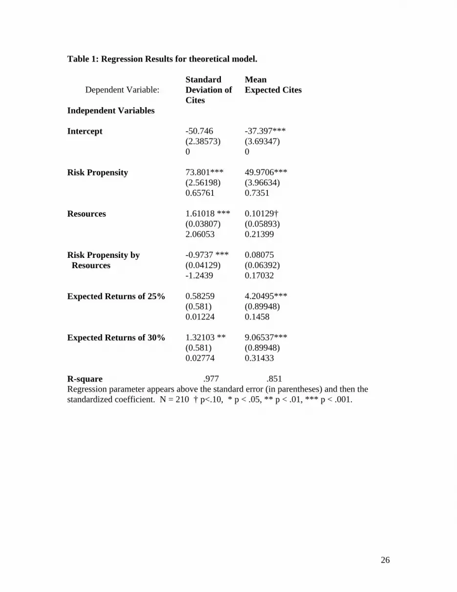
Because risk propensity and resources interact to influence the outcomes, we used

regression to interpret the model predictions. The results appear in Table 1. The

explanatory variables are risk propensity, resources available, the interaction of risk

propensity by resources available, and finally, dummy variables for expected returns of

25 and 30 percent:

Y = b0 + b1 RiskPropensity + b2 Resources + b3 Resources * RiskPropensity

+ b4 ExpectedReturns25%Dummy + b5 Expected Returns30%Dummy + e (7)

where Y can be either the mean citations or the standard deviation of citations.

Applying regression to these data provides a heuristic for interpretation. Because the

data come from an inherently deterministic process, the regression coefficients and their

12

standard errors do not have the normal statistical interpretations. While in the discussion

below we do consider statistical significance, we recognize this as a heuristic. 2

Table 1 presents the regression results on expected citations and standard deviation in

expected citations from the model solutions. Within this model, we allow for the

possibility that the impact of Risk Propensity on citations depends on the level of

Resources (as represented by the interaction of Risk Propensity and Resources). That is,

Equation 7 can be rewritten as:

Y = b0 + (b1 + b3 Resources) * RiskPropensity + b2 Resources

+ b4 ExpectedReturns25%Dummy + b5 Expected Returns30%Dummy + e (8)

The influence of Risk Propensity on Y thus depends on {b1 + b3 Resources}. The

statistical test requires consideration of the total variance of this equation, rather than

simply the variance of the parameters individually. A symmetric analysis gives similar

results for the influence of Resources on the dependent variable. We used the approach

noted in Friedrich (1982) to estimate total effects and their statistical significance.

Risk Propensity and Resources both positively and significantly influence expected

citation rates. Their interaction, however, was not significant. This leads to the

following hypotheses:

2 Earlier work (Bromiley and Fleming 2000) also ran tobit models that demonstrated no substantive differences in results. We retain the basic regression models for ease of interpretation.

13

H1: Risk Propensity positively influences expected citations. H2: Resources positively influences expected citations.

The results for the standard deviation of expected citations are slightly more complex

because the interactions demonstrated significance. Risk Propensity positively influences

expected citations for low levels of Resources but the influence declines and becomes

negative for higher levels of Resources. The influences are statistically significant across

most of the range of Resources. Resources positively influence expected citations but the

magnitude of the influence declines for higher levels of Risk Propensity (although

remaining positively and statistically significant even at high levels of Risk Propensity).

This leads to the following hypotheses:

H3: At low levels of Resources, Risk Propensity positively influences the standard

deviation of expected citations. H4: The influence of Risk Propensity on the standard deviation of expected citations

declines with Resources and becomes negative for high levels of Resources. H5: Resources positively influence the standard deviation of expected citations. H6: The magnitude of Resources' influence on the standard deviation of expected

citations decreases with the level of Risk Propensity.

14

Data and Measures An empirical test of the model requires specification of the measures for the quality of a

firm’s inventions, Risk Propensity, Resources, and control variables. To these we now

turn.

Invention Quality We analyze the patents granted to publicly traded U.S. firms during the

months of May and June of 1990, downloaded from the Micro Patent product. The

dependent variable of citations came from a count of prior art citations from patents over

the future 6 years and 5 months.3 We identified the CUSIP number associated with each

firm and downloaded firm characteristics such as sales and R&D investment from

Compustat for each firm in the years prior to patent application. Use of current

Compustat database introduces a public ownership, size, and survival bias. While we

made use of historical data in Compustat (that is, we included data on dead firms or those

whose name had changed or since acquired), we are currently broadening our data

gathering efforts to correct any remaining survival bias. The research assistants only

identified exact matches between the patent assignee and Compustat CUSIP, i.e., they did

not identify subsidiaries or conglomerates. This ensures the most accurate association

between observed firm characteristics and patent citation data.

The model only considers the technological success of firm search strategies and does not

consider a firm’s ability to profit from its inventions. As such, the empirical test should

3 We chose this period to make maximal use of our data that end in November of 1996. This period should capture the bulk of citations to a patent as these citations typically peak within six years from the grant date (Hall, Jaffe, and Trajtenberg 2000). While there appears to be strong correlation between the rates of early and later citations to a patent, researchers are actively pursuing the topic (Hall, Jaffe, and Trajtenberg 2000).

15

separate invention and innovation, that is, the difference between generating a new

technology and profiting from it (Schumpeter 1939 pg. 85). Much work has

demonstrated that patents that receive greater number of future art citations are more

important technologically (Hall, B. and A. Jaffe, M. Trajtenberg 2000). While this work

has also demonstrated a positive correlation between citations and social and economic

value, we do not consider such issues in the current work, or the relationship between

highly cited patents and firm valuation and technology commercialization. We refer the

reader to recent work on this topic (Deng, Lev, and Narin 1999).

Risk Propensity Behavioral work in organizational economics provides a model of risk

propensity. Cyert and March (1992) assume that firms have a level of performance to

which they aspire (an aspirations level) and a level they actually achieve. The level of

aspirations depends largely on comparison to other firms in the industry. Thus, a

regulated utility perceives its performance as inadequate if it earns less than comparable

utilities, while a software company compares itself to other software companies. Cyert

and March's (1992) behavioral theory of the firm predicts that firms that perform below

their aspiration levels will search for ways to improve. Furthermore, firms that perform

well above their aspiration levels will also take risks because they can afford to do so

without risking falling below their aspiration level. In the R&D realm, such search

involves moving R&D activities to riskier but potentially more profitable activities. In

other words, a firm's distance below its reference point strongly, positively influences its

risk propensity while a firm's distance above its reference point moderately, and

positively influences its risk propensity.

16

Much of the behavioral literature uses industry mean return on assets as a firm's reference

point (Fiegenbaum and Thomas, 1986; 1988). Basically, the firm compares its return on

assets to the industry mean. Due to the influence of small and usually loss making firms,

we found that the industry mean was typically negative. As a result, almost all of our

firms performed above average. To reduce this influence of small negative outliers, we

used the industry median. Both aspiration measures gave similar results.

We therefore include the difference between a firm's performance (return on assets) and

its industry's median return on assets as an indicator of risk propensity, as measured in

the years prior to patent application, and differentiate between cases where the firm is

above or below the industry median. We calculated ROA as income before extraordinary

expenses divided by total assets, for each firm and its industry average. Compustat three

digit SIC codes provided the firm’s industry and enabled comparison to other firms with

the same three digits. The data gathering process resulted in a total of 371 different

firms, with 729 patents from firms below their industry median and 1863 from firms

above. The preponderance of above median firms may indicate a survival bias, or that

firms that patent are more technologically advanced and innovative. Such firms probably

do better in their industry, relative to firms that do not patent.

Resources have a straightforward representation as funds allocated to research and

development. The interaction of Resources and Risk Propensity is simply R&D spending

times distance from industry median.

17

Controls We include two controls. Size may influence citations to patents, because large

and higher status firms are more likely to be cited (Podolny and Stuart 1995). We control

for differences in firm size by including firm sales in the year of patent application.

Patent practices also vary across technologies. Following the logic of fixed-effects

modeling, the models include a control for differences in the mean and variance of

citation rates across technology classes. Computation of both the technology mean and

variance controls proceeds with similar two-step processes. In the first step, we calculate

the average number of citations that each patent in a particular class receives from patents

granted between January of 1985 and June of 1990 (9).4 If all patents belonged to only

one class, we could use this measure to control for differences in citation likelihood

across classes, but most patents fit in more than one class. In the second step, we weight

this term according to a patent’s class assignments (equation 10) where p indicates the

proportion of patent k’s sub-class memberships that fall in class i. Calculating the

technology variance control follows a nearly identical process detailed in (11,12). While

this control variable will vary across industries and correlate with industry membership, it

is actually superior to an explicit industrial control, because most firms straddle multiple

industries. Tables 2 and 3 list descriptive and correlation statistics.

iji ij

j

i class-subin patents ofCount

7/90) (before Citations classpatent in citations Average

∑∈=≡ µ (9)

Technology mean control patent k M pk ik i≡ = µ (10)

4 We allow all patents issued between January 1985 and June 30, 1990 to enter the estimation of the technology controls. This means that the patents used to calculate the technology controls vary in the time during which they can receive citations. Alternatively, we could select a small set of patents from 1985 and base the measures on the subsequent five years of citations; however, this approach would ignore the patent activity just prior to our sample.

18

( )

iji ij

j

i class-subin patents ofCount

-7/90) (before Citations classpatent in arianceCitation v

2i

2∑

∈=≡µ

σ (11)

Technology variance control patent k V pk ik i≡ = σ 2 (12)

Empirical Model

We estimated the predictions of our model on the mean expected citation rate and

variance in citation rate. The dependent variable of citation counts takes on only whole

number values (that is, 0,1,2, etc.). Use of a linear regression model on such data could

yield inefficient, inconsistent, and biased coefficient estimates (Long 1997). Explicit

count models can avoid these problems. Researchers often use Poisson models to

analyze count data, but Poisson models assume that the mean and variance of the

observed distribution are equal. These data, like most count data, exhibit over-dispersion

– the variance is greater than the mean. Negative binomial regressions explicitly

accommodate this over-dispersion, however, by enabling the variance to be greater than

the mean. Recent developments (King 1989, Jorgensen 1997) also support independent

estimation of effects on the mean, and the variance of the predicted mean, as functions of

potentially differing sets of variables.

To begin with, consider a model that estimates the mean number of citations that a patent

should receive, given its independent variables. The observed citations to the patent will

not correspond exactly to the prediction, however, and will be distributed with some

19

variance around the expected mean. We operationalize the variance in quality of

invention by estimating the effects of substantive variables on this variance.

Most derivations of the negative binomial start from a basic Poisson model (13). The

basic Poisson model estimates the probability of an observed count, conditional on an

expected mean iµ . To avoid negative (i.e., undefined) expected values for the mean iµ ,

Poisson models typically parameterize explanatory variables as an exponential function

(14). The method of maximum likelihood is then applied to the joint frequency formed

from the product of the marginal frequencies of (13), to determine the coefficient values

that are most likely to result in the observed counts.

(13) !

)|Pr(i

yi

ii yey

ii µµ−

=x

(14) )|( )( βµ ixiii eyE ==x

The negative binomial model replaces the Poisson mean iµ with the random variable i

~µ

(15). This replacement enables the inclusion of an error term ieiεδ = and allows the

predicted mean to vary according to the distribution of the error term. Substitution of

i

~µ for iµ in (13) results in (16).

(15) )(~

iix

iiie δµµ εβ == +

(16) !

)(),|Pr(

i

yii

iii ye

yiii δµ

δδµ−

=x

20

When i

~µ replaces iµ in (16), the probability of the observed count becomes conditional

on the error distribution. This conditioning can be removed, however, by specifying the

error distribution and integrating with its probability density function to obtain the

marginal density. Most formulations specify a gamma distribution for iδ with parameter

iν and probability density function )( ig δ as in (17) (Hausman, Hall, and Griliches 1984,

Cameron and Trivedi 1986, King 1989, Long 1997). Although the error term can take

other distributions, this parameterization is flexible, computationally tractable, and can be

derived from a variety of assumptions. While other versions of the gamma distribution

take two parameters, this derivation (from Long 1997 pg. 232) sets both to iν , which

forces the mean of iδ equal to one and the variance of iδ equal to iν/1 . Integrating (16)

with the density function of (17) gives the probability of the negative binomial of (18),

which is then conditional only on independent variables ix .

(17)dt et)( and 0, for e )(

)( t-

0

1-i

)(- ii1 ∫∞

=Γ>Γ

= − ννδνν

ννδν

νδ ii

ii

iig

(18) )()()(!)()|Pr( ii y

ii

i

ii

i

ii

iiii y

yyµν

µµν

ννν ν

++Γ+Γ

=x

While the first term of (15) fully specifies the mean of the negative binomial, various

parameterizations of iν remain possible. Cameron and Trivedi (1986) propose the

negative binomial II parameterization (or Neg Bin II) when the variance/mean ratio of the

observed data is linear in the mean. By contrast, the Negbin I holds the variance/mean

ratio constant. The Neg Bin II specification is also much more robust to distributional

21

misspecification than other parameterizations (Cameron and Trivedi 1986). 5

Equation (19) specifies the Neg Bin II parameterization of the conditional variance. iα is

the inverse of iν and is parameterized as an exponential function, similar to the mean

specification but with potentially different variables. Since iii ανδ == /1)var( , greater

variance of the error term will result in an increase of iα . Variables that decrease α will

decrease the variability of inventive outcomes. STATA estimates (18) by the method of

maximum likelihood. This technique estimates both the mean iµ and variance iν/1 from

(18), and hence produces only a single log likelihood.

(19) )1()|( 2ii

i

iiiyVar αµµ

νµ

µ +=+=x

Results

Table 4 lists the results of the negative binomial model estimation. Stata provides a

robust estimator (White 1980, Rogers 1993) that controls for the lack of independence

between observations of multiple patents from a single firm. This deflates standard errors

and allows for firm differences. For example, assuming that firm patenting policies

remain stable over the years of observation (88% of patents were applied for in 1988 and

5 We verified use of the quadratic formulation by linear regression of

citationspredictedcitationspredictedcitations

) ( 2− on predicted citations from a simple Poisson model. This

regression estimated the coefficients of the constant and regressor as 4.78 (1.89) and .302 (.291), indicating an over-dispersed Poisson whose variance does not significantly exceed a linear scaling of the mean (i.e., the relationship between the mean and variance may be constant). Although the 95% confidence interval of the regressor [-.27, .87] includes 0, all previous analyses of the larger dataset (all 17,264 patents of May and June of 1990) did not. Hence we are reluctant to abandon the Neg Bin II but will also estimate the Neg Bin I.

22

1989 and the remainder in years prior to that), then the cluster command would control

for differences in patenting policies across firms. The largest cluster of patents comprises

137 patents or 5.3% of the sample, and hence does not violate the small sample

assumptions of the estimator (Rogers 1993). Exploratory analyses did not reveal any

significant non-linear relationships. Given that the lagged effect of research and

development spending is not clear (Hausman, Hall, and Griliches 1984), we include

separate models of lagged years prior to the year of patent application. Model 3 includes

the variables from three years prior to the patent application, model 4 from two years, and

model 5 from the year prior to application. The coefficient estimates in the mean are

stable across the different lag structures, with the exception of the interaction effect

between below industry median firms and R&D spending. In our analyses below, we

will consider mainly the results from model 5, for the year immediately prior to the patent

application.

Examining the results on mean patent citation counts, we find a strong positive influence

of distance from industry median ROA. The effects for being below and above are

roughly comparable. For firms below industry median ROA, lowering their ROA

increases the subsequent citation rate to their patents (parameter of 1.80, p<.05). A one

standard deviation increase below the median increases the expected patent citation count

by 6.4%. 6 Over the entire range of the variable, the expected count increases 133%. For

firms above industry ROA, increasing their ROA also increases the subsequent citation

rate to their patents (parameter of 1.9, p<.01). A one standard deviation increase below

6 From the coefficient estimate of model 5 and standard deviation of the variable: .064.1)0345.0*7972.1( =e

23

the median increases the expected patent citation count by 10.6%. Over the entire range

of the variable, the expected count increases 100%. These results agree with the model's

representation of the impact of risk propensity and the use of an aspirations model to

represent risk propensity.

In further support of the model, we find a strong positive influence of R@D spending

upon mean citation counts (parameter of 0.19, p<.05). A one standard deviation increase

in spending results in a 22% increase in citations. Over the entire range of the variable,

the expected count increases 138%. Although not predicted by the theory model, we also

find a strong and negative interaction effect between aspiration and resources. For firms

below their industry median, the interaction of distance and spending has a negative

effect (parameter of –1.28, p<.001). The interaction is stronger for firms above

(parameter of –2.74, p<.001). It appears the effects of risk propensity and resources

become much less as the other variable increases. A tobit model for the mean citation

count returned similar substantive results as the negative binomial dispersion model,

although some significance levels changed.

The estimates for the dispersion returned generally insignificant and contrary results.

Only the below industry median estimate was significant in model 5 (parameter of –3.18,

p<.05) and in the opposite direction to the model’s predictions. At the mean of citations

and the conditional mean of the variable, a one standard deviation increase in the variable

24

would result in a decrease of 13.5% in the variance of citations. 7 The influence of firm

R@D was also consistently negative although generally not significant. Interestingly, it

had its strongest and most significant effect in model 3, for the three year lag, where a

one standard deviation increase would decrease the variance by 21.2%. This result is

consistent with arguments that research and development spending is mostly aimed at

reducing technology to practice (Rosenberg 1990). Previous estimates of all the original

patents in this dataset have returned very significant interaction effects in the dispersion

parameter (Fleming and Sorenson 2001). Those models used 17,264 data points,

however, and thus provide additional evidence that patent citation data are extremely

noisy (Scherer and Harhoff 2000).

Conclusion

We presented a formal model that predicts mean citations and variance in citations to a

firm’s patents, based on a firm’s Risk Propensity and R&D Resources. We measured a

firm’s Risk Propensity as its absolute distance from industry median ROA in the years

prior to patent application. We measured R&D Resources as R&D investment and

estimated effects with negative binomial dispersion models.

The empirical results indicate that the underlying model correctly predicts the positive

effects of risk propensity and resources on the mean of citations to a firm’s patents.

7 The variance at the mean citation count of 5.03 and the conditional mean of below industry median (0.0393) would have been 12.31]03.5[03.5 2)0393.0*797.1()0393.0*179.3()0393.0*797.1(2 =+=+ − eeeαµµ . At one standard deviation more, the variance would be:

93.26]03.5[03.5 2))0559.00393.0*(797.1())0559.00393.0*(179.3())0559.00393.0*(797.1(2 =+=+ ++−+ eeeαµµ . (31.12-26.93)/31.12 = 13.5%.

25

Although the theory model did not predict a significant interaction effect, the empirical

results indicated a strong and negative interaction between risk propensity and resources.

The hypothesized effects on the dispersion of citation counts were not supported,

however, and in some cases were contrary to predictions. While the possibility of the

measures being flawed merits investigation, we note that the measures do have strong

associations with the dependent variables – the model explains significant portions of the

variation in the dependent variables even if the parameters do not always have the

expected signs. This suggests a need for an alternative theoretical approach to

understanding the influence of Risk Propensity and Resources on citations, and in

particular, the dispersion of citations.

The model, data, and empirical method provide a rich basis for future investigations

regarding the mean and variance of inventive search. For example, the patents of firms

that take more inventive risks might be more highly cited, but these citations depend on

the firm first receiving a patent. Will greater risk taking result in fewer, but more highly

cited patents? The citation payoff could be modeled stochastically, since even if a project

results in a patent, the patent’s success cannot be accurately predicted. Aspiration points

can also be empirically investigated, for example, whether firms compare themselves to

other firms or their recent past performance (Greve 1998). Future work with patent

citation count data and negative binomial decomposition models will ultimately enable

research into the outliers of technological breakthroughs, events that many have

previously argued are unpredictable and therefore not amenable to rigorous study.

26

Table 1: Regression Results for theoretical model.

Dependent Variable:

Independent Variables

Standard Deviation of Cites

Mean Expected Cites

Intercept -50.746 -37.397*** (2.38573) (3.69347) 0 0 Risk Propensity 73.801*** 49.9706*** (2.56198) (3.96634) 0.65761 0.7351 Resources 1.61018 *** 0.10129† (0.03807) (0.05893) 2.06053 0.21399 Risk Propensity by -0.9737 *** 0.08075 Resources (0.04129) (0.06392) -1.2439 0.17032 Expected Returns of 25% 0.58259 4.20495*** (0.581) (0.89948) 0.01224 0.1458 Expected Returns of 30% 1.32103 ** 9.06537*** (0.581) (0.89948) 0.02774 0.31433 R-square .977 .851 Regression parameter appears above the standard error (in parentheses) and then the standardized coefficient. N = 210 † p<.10, * p < .05, ** p < .01, *** p < .001.

27

Table 2: Summary statistics mean sd min maxCitations 5.03 6.09 0.00 58.00Mean technology control 1.29 0.43 0.35 3.03Variance technology control 5.40 2.87 0.36 20.55Firm sales in year of application control 17.59 25.03 0.00 124.99Above industry median ROA dummy 0.72 0.45 0.00 1.00Distance below industry median ROA 0.01 0.03 0.00 0.47Distance above industry median ROA 0.04 0.05 0.00 0.36Firm R&D 0.72 1.08 0.00 4.75Distance below median * Firm R&D 0.01 0.03 0.00 0.29Distance above median * Firm R&D 0.02 0.05 0.00 0.34

Table 3: Correlation matrixCites Mean Variance Sales Dummy Below Above R&D Below*R&D

Mean technology control 0.32Variance technology control 0.31 0.94Firm sales control 0.01 0.12 0.09Above industry median ROA dummy 0.03 -0.01 -0.01 -0.29Distance below industry median ROA 0.01 0.04 0.03 -0.04 -0.51Distance above industry median ROA 0.07 -0.03 0.02 -0.20 0.48 -0.25Firm R&D 0.06 0.23 0.20 0.90 -0.19 -0.03 -0.09Distance below median * Firm R&D 0.03 0.12 0.09 0.30 -0.32 0.37 -0.16 0.34Distance above median * Firm R&D 0.06 0.22 0.23 0.30 0.28 -0.14 0.37 0.57 -0.09

28

Table 4: Negative binomial dispersion models of citation counts to patents granted in May and June 1990 (all variables except controls lagged as indicated from year of patent application, +p<0.01, *p<0.05, **p<0.01, ***p<0.001, stnd errors in parantheses, robust estimation adjusted on firm).

Model 3 Model 4 Model 5(year t - 3) (year t - 2) (year t - 1)

mean parametersMean technology control 0.8214*** 0.8284*** 0.8751***

(0.0730) (0.0669) (0.0665)

Firm sales in year of application control -0.0035 -0.0028 -0.0038(billion $) (0.0023) (0.0020) (0.0025)

Above industry median ROA dummy 0.0439 0.0222 0.1605*(0.0788) (0.0816) (0.0812)

Distance below industry median ROA 1.9899** 2.0089* 1.7972*(absolute value) (0.7357) (0.8377) (0.7388)

Distance above industry median ROA 2.5989** 2.6614*** 1.9124**(0.8377) (0.8024) (0.6346)

Firm R&D (billion $) 0.1687* 0.1164+ 0.1825*(0.0818) (0.0680) (0.0749)

Distance below median * Firm R&D -1.0611 1.1521 -1.2785***(0.9326) (0.9013) (0.3777)

Distance above median * Firm R&D -1.7882** -1.7463** -2.7391***(0.6013) (0.6289) (0.7130)

Constant 0.3151** 0.3409** 0.2002+(0.1207) (0.1107) (0.1145)

dispersion parametersVariance technology control -0.0231 -0.0288* -0.0286*

(0.0145) (0.0139) (0.0134)

Firm sales in year of application control 0.0081+ 0.0059 0.0055(billion $) (0.0045) (0.0044) (0.0049)

Above industry median ROA dummy -0.2650* -0.0242 -0.0049(0.1222) (0.1171) (0.1479)

Distance below industry median ROA -2.2492 -1.4783 -3.1794*(absolute value) (1.5970) (1.2924) (1.5612)

Distance above industry median ROA 1.1145 0.6600 -0.0358(0.9927) (0.8368) (0.8074)

Firm R&D (billion $) -0.2920+ -0.2216 -0.1841(0.1533) (0.1374) (0.1314)

Distance below median * Firm R&D -1.7199 1.9147 0.4898(1.8480) (1.4621) (0.6719)

Distance above median * Firm R&D 0.6673 0.4163 0.3253(0.9982) (1.1564) (1.1027)

Constant 0.1704 0.0398 0.0724(0.1374) (0.1239) (0.1522)

log likelihood -5899.71 -6577.39 -6828.7n 2249 2489 2592

29

References Albert, M. B. and F. Narin, D. Avery, P. McAllister (1991), "Direct Validation of Citation Counts as Indicators of Industrially Important Patents," Research Policy; 20:251-259. Bromiley, P. and L. Fleming (2000), "A Positive Model of Allocation of Research Expenditure Allocation," under submission and available from lfleming@hbs.edu.

Cameron, A. and P. Trivedi (1986) “Econometric Models Based on Count Data: Comparisons and Applications of Some Estimators and Tests, Journal of Applied Econometrics, Vol. 1: 29-53. Cohen, W. and S. Klepper (1996), “Firm Size and the Nature of Innovation within Industries: The Case of Process and Product R&D,” The Review of Economics and Statistics, pp. 232-243. Cyert, R. and J. March (1992), A Behavioral Theory of the Firm, Blackwell Publishers Ltd. Oxford. Deng, Z. and B. Lev, F. Narin (1999), “Science and technology as predictors of stock performance”, Financial Analysts Journal, Charlottesville, Vol. 55, Iss. 3; pg. 20-33. Fleming, L. (forthcoming), “Recombinant Uncertainty in Technological Search,” forthcoming in Management Science, January 2001. Fleming, L. and O. Sorenson (2001), “Science, Technological Interdependence, and Invention,” working paper available from the first author. Fiegenbaum, A., & Thomas, H. (1986), "Dynamic and risk measurement perspectives on Bowman's risk-return paradox for strategic management: An empirical study," Strategic Management Journal, 7: 395-407. Fiegenbaum, A., & Thomas, H. (1988), "Attitudes toward risk and the risk-return paradox: Prospect theory explanations," Academy of Management Journal, 31: 85-106. Friedrich, R. (1982), “In Defense of Multiplicative Terms in Multiple Regression Equations,” American Journal of Political Science, 26:4:797-833. Greve, H. (1998), “Performance, aspirations, and risky organizational change,” Administrative Science Quarterly, 43:1: 58-77. Hall, B. and A. Jaffe, M. Trajtenberg (2000), “Market Value and Patent Citations: A First Look,” NBER Working Paper 7741. Hausman, J. and B. Hall, Z. Griliches (1984), “Econometric Models for Count Data with an Application to the Patents-R&D Relationship,” Econometrica, 52: 909-938. Henderson, R. and I. Cockburn (1996), “Scale, scope, and spillovers: the determinants of research productivity in drug discovery,” Rand Journal of Economics, Spring, pp. 32-59. Jensen, M. and Meckling, W. (1976), “Theory of the firm: Managerial behavior, agency costs and ownership structure,” Journal of Financial Economics, 3, 305-360. Jorgensen, B. (1997), The Theory of Dispersion Models, Chapman and Hall, London.

30

Kahneman, D. and D. Lovallo (1993), 'Timid decisions and bold forecasts: A cognitive perspective on risk taking', Management Science, Vol. 39, pp. 17-31. King, G. (1989), “Event Count Models for International Relations: Generalizations and Applications,” International Studies Quarterly, 33:123-147. Long, J. (1997), Regression Models for Frequency and Count Data, London, Sage Publications. Mansfield, E. and J. Rapoport, A. Romeo, S. Wagner, G. Beardsley (1977), “Social and Private Rates of Return from Industrial Innovations,” Quarterly Journal of Economics, vol. 91:2:221-240. March, J. and Z. Shapira (1992), “Variable Risk Preferences and the Focus of Attention,” Psychological Review, 99:1:172-183. Podolny, J. and T. Stuart (1995), "A Role Based Model of Technological Change," American Journal of Sociology, Volume 100, no. 5, pp. 1224-1260. Rogers, W. (1993), “Regression standard errors in clustered samples,” Stata Technical Bulletin, 13: 88-94. Rosenberg, N. (1990), “Why do firms do basic research?” Research Policy 19:165-174. Scherer, F. and D. Harhoff (2000), “Technology Policy for a world of skew-distributed outcomes,” Research Policy, 29:559-566. Schumpeter, J. (1939), Business Cycles, New York, McGraw-Hill Book Company, Inc. Sorenson, J. and T. Stuart (2000), “Aging, Obsolescence, and Organizational Innovation,” Administration Science Quarterly, forthcoming. Trajtenberg, M. (1990), “A Penny for Your Quotes: Patent Citations and the Value of Innovations,” Rand Journal of Economics, 21(1), pp. 172-187. Trajtenberg, M., Henderson, R., and A. Jaffe (1997), “University Versus Corporate Patents: A Window on the Basicness of Invention,” Economic Innovation and New Technology, Vol. 5: 19-50. Tversky, A. and D. Kahneman (1992), “Advances in Prospect Theory: Cumulative Representation of Uncertainty," Journal of Risk and Uncertainty, 5, pp. 297-323. White, H. (1980), “Heteroskedasticity-Consistent Covariance Matrix Estimator and a Direct Test of Heteroskedasticity,” Econometrica, 48:4:817-838.