Aberrations in curved x-ray multilayers

Ch. Morawe*a, J-P. Guigaya, V. Mocellaa,b, C. Ferreroa, H. Mimurac, S. Handac, K. Yamauchic aESRF, F-38043 Grenoble, France bCNR-IMM, I-80131 Napoli, Italy

cOsaka University, Osaka 565-0871, Japan

ABSTRACT

Aberration effects in curved multilayers for hard X rays are studied using a simple analytical approach. The method is based on geometrical ray tracing including refraction effects up to the first order of the refractive index decrement �. The interpretation of the underlying equations provides fundamental insight into the focusing properties of these devices. Using realistic values for the multilayer parameters the impact on spot broadening and chromaticity is evaluated. The work is complemented by a comparison with experimental focusing results obtained with a W/B4C multilayer mirror.

Keywords: X-ray optics, x-ray multilayers, nano-focusing, aberrations

1. INTRODUCTION Recent years have seen a rapid evolution in hard x-ray optics, particularly boosted by the use of extremely brilliant 3rd generation synchrotron radiation sources. X-ray beams were focused down to spots below 50 nm using various optical elements such as Fresnel Zone Plates (FZPs) [1], Compound Refractive Lenses (CRLs) [2], Wave Guides (WGs) [3], capillary optics [4], curved Total Reflection Mirrors (TRMs) [5,6], transmission Multilayer Laue Lenses (MLLs) [7,8], and Reflective Multilayers (RMLs) [9]. The question arose, whether the ultimate spatial resolution of x-ray optical elements is limited by physical properties other than the wavelength and the numerical aperture. Several theoretical studies, mainly numerical wave optical calculations, were published treating the cases of FZPs [10], CRLs [11], TRMs [12,13], and MLLs [14,15]. Advanced numerical ray tracing calculations have been applied to RMLs [16]. Alternatively, a purely analytical approach was proposed [17,18]. This work will resume and update the outcome of these analytical investigations.

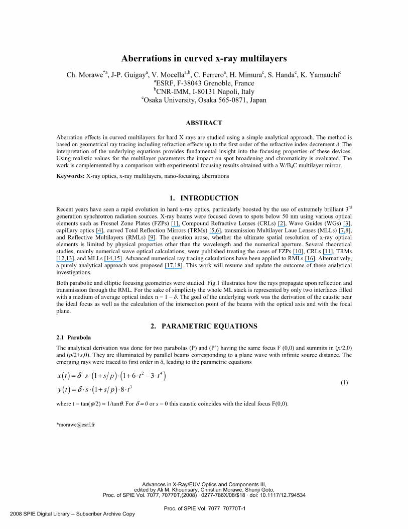
Both parabolic and elliptic focusing geometries were studied. Fig.1 illustrates how the rays propagate upon reflection and transmission through the RML. For the sake of simplicity the whole ML stack is represented by only two interfaces filled with a medium of average optical index n = 1 – �. The goal of the underlying work was the derivation of the caustic near the ideal focus as well as the calculation of the intersection point of the beams with the optical axis and with the focal plane.

2. PARAMETRIC EQUATIONS 2.1 Parabola

The analytical derivation was done for two parabolas (P) and (P’) having the same focus F (0,0) and summits in (p/2,0) and (p/2+s,0). They are illuminated by parallel beams corresponding to a plane wave with infinite source distance. The emerging rays were traced to first order in �, leading to the parametric equations

( ) ( ) ( )( ) ( )

2 4

3

1 1 6 3

1 8

x t s s p t t

y t s s p t

δ

δ

= ⋅ ⋅ + ⋅ + ⋅ − ⋅

= ⋅ ⋅ + ⋅ ⋅ (1)

where t = tan(ϕ/2) ≈ 1/tanθ. For δ = 0 or s = 0 this caustic coincides with the ideal focus F(0,0).

*morawe@esrf.fr

Advances in X-Ray/EUV Optics and Components III,edited by Ali M. Khounsary, Christian Morawe, Shunji Goto,

Proc. of SPIE Vol. 7077, 70770T,(2008) · 0277-786X/08/$18 · doi: 10.1117/12.794534

Proc. of SPIE Vol. 7077 70770T-12008 SPIE Digital Library -- Subscriber Archive Copy

P n=1-5

n10

M

Fig.1: Ray propagation through the curved layered structure. For simplicity, only the parabolic approximation is shown. One ray is reflected from the upper ML surface reaching the ideal focus F. Another ray is first refracted when crossing P in point C, then reflected in point N on P’, and again refracted when crossing P in point D. The curve pointing to F illustrates the resulting envelope of all rays reflected from P’. The polar angle � is defined by the virtual ray reflected in point N without refraction in the ML medium (broken line). The dimensions are not to scale.

2.2 Ellipse

The treatment for a finite source distance and a cylindrical wave front requires two confocal ellipses with focuses in S and F and different eccentricities e and e’. The derivation leads to a set of extended algebraic equations. For eccentricities close to 1, however, the solutions for the caustic converge to the parabolic case (1) [17].

For the sake of simplicity, the following discussion will be based on equations (1).

3. INTERPRETATION OF THE RESULTS Two fundamental cases may be considered to interpret equations (1):

1. Aberrations due to a single interface illuminated at variable angles of incidence where � = const and s = const, while t ranges from t1 to t2 , representing the mirror edges.

2. Aberrations originating from interfaces at variable penetration depths at a given angle of incidence where t = const, while s ranges from 0 (top surface) to smax , given by the extinction depth z of the multilayer.

3.1 Single interface aberrations

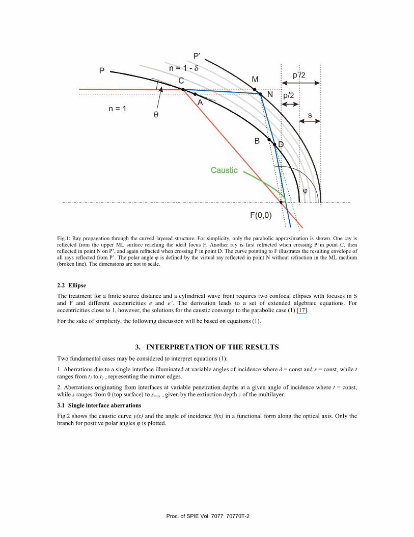
Fig.2 shows the caustic curve y(x) and the angle of incidence �(x) in a functional form along the optical axis. Only the branch for positive polar angles � is plotted.

Proc. of SPIE Vol. 7077 70770T-2

0

100

200

300

400

0

0.5

1

1.5

2

-1 105 -8 104 -6 104 -4 104 -2 104 0

y [n

m]

Grazing angle Θ

[deg]

x [nm]

E = 24550 eVP = 150 mQ = 0.077 mδ = 2.7e-6

p = 5775 nms = 0.253 nm

0

1 10-5

2 10-5

3 10-5

4 10-5

20

30

40

50

60

70

80

90

-1 10-5 -5 10-6 0 5 10-6

Fig.2: Positive branch of the caustic curve y(x) (left scale) and corresponding grazing incidence angle θ(x) (right scale). The insert zooms into the zone around the ideal focus and the corresponding angles of incidence.

The behaviour close to the ideal focal point F(0,0) is illustrated in the insert of Fig.2. The small zero x-offset of

( ) ( )2 1x s s pθ π δ= = ⋅ ⋅ +

at normal incidence can be confirmed using Gaussian optics and the classical conjugation formulas on a sequence of the involved optical surfaces. Obviously, the effect disappears for � = 0 or s = 0.

3.2 Variable penetration

Case 2 can be approximated analytically from equations (1). At a given position on a curved mirror at grazing incidence, the polar angle variation due to variable beam penetration is of the order of

610ϕϕ

−∆ ≈

In the present calculation, t can therefore be considered as constant with depth and s << p for all s. Eliminating the corresponding terms in equations (1) one obtains

( )3

2 4

81 6 3

ty x xt t⋅= ⋅

+ ⋅ − ⋅ (2)

At a given angle of incidence the caustic can therefore be approximated by a straight line through the ideal focus. In other words, both s and � essentially amplify the angular effect at a given location on a curved ML mirror.

Proc. of SPIE Vol. 7077 70770T-3

4. GRAPHICAL REPRESENTATION It is helpful to calculate the trajectories of some rays for a given penetration parameter s. The corresponding equations (2) and (3) in reference [17] can be simplified and for small grazing angles one obtains for the intersection points X(Y=0) with the optical axis and Y(X=0) with the focal plane

( )( )

2 4 4

3 3

( 0) 1 2

( 0) 2 2 2

X Y s t t s t

Y X s t t s t

δ δ

δ δ

= ≈ ⋅ ⋅ + ⋅ + ≈ ⋅ ⋅

= ≈ ⋅ ⋅ ⋅ ⋅ + ≈ ⋅ ⋅ ⋅ (3)

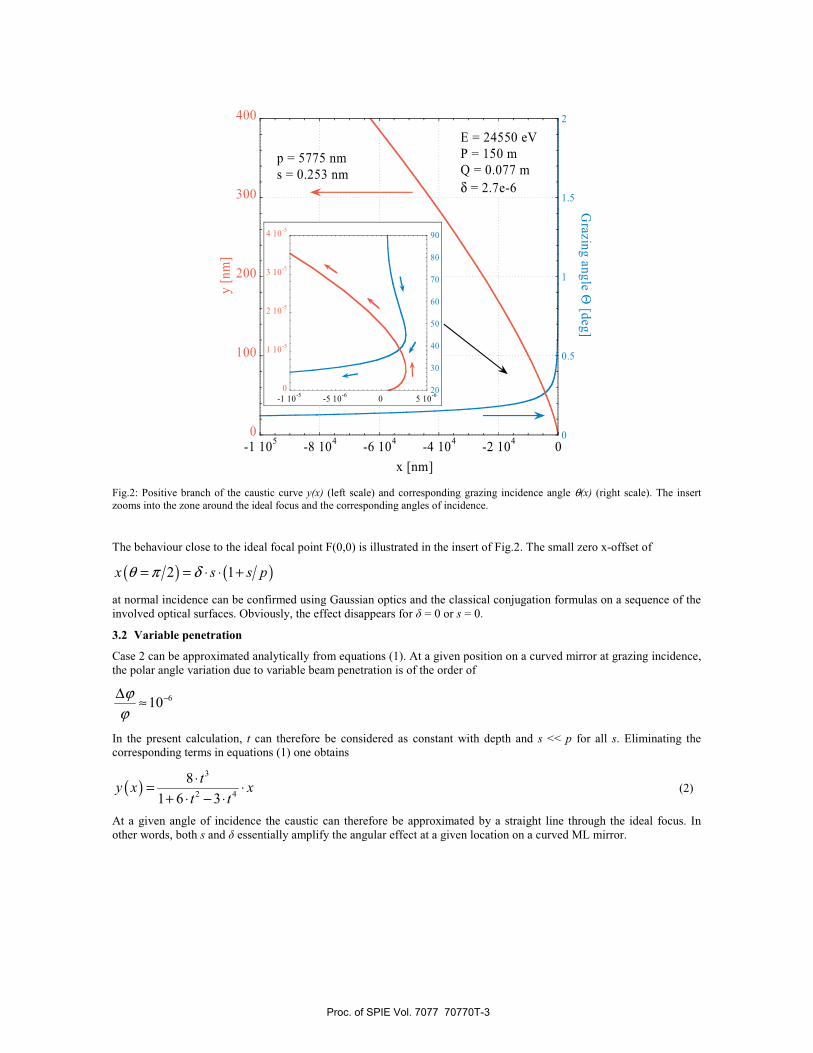
Note that equations (1) and (3) have a very similar structure and their leading terms go with the same power in t. Fig.3 shows how the rays are located with respect to the caustic. Each ray (arrows) is tangential to the caustic (underlying curve) at the point where the latter intersects with the line corresponding to the local grazing angle (broken lines).

0

10

20

30

40

50

-3000 -2000 -1000 0 1000

y [n

m]

x [nm]

θ = 0.30 deg0.35 deg0.40 deg0.45 deg

E = 24550 eVP = 150 mQ = 0.077 mδ = 2.7e-6p = 5776 nms = 0.25 nm

Focalplane

Fig.3: Family of rays (arrows) emerging from a curved RML with constant penetration parameter s but variable grazing angles. The underlying curve is the corresponding caustic. The straight broken lines indicate positions of constant incidence angles.

The intersection points with the focal plane and with the optical axis are plotted in Fig.4 as a function of the grazing angle and for the same parameter set as in Fig.3. The deviation X of the focal length along the optical axis is shown on the left scale, aberrations Y in the focal plane on the right. Calculations using equations (3) are represented by solid lines. The broken lines show exact numerical calculations. As expected, both sets of curves are in very good agreement, except for angles near the critical angle, where the linear approximation in the derivation of equations (1) and (3) fails. Note that X is typically two orders of magnitude larger than Y.

Proc. of SPIE Vol. 7077 70770T-4

0

500

1000

1500

2000

0

5

10

15

20

0.2° 0.3° 0.4° 0.5° 0.6°

Opt

ical

axi

s X [n

m] Focal plane Y

[nm]

Grazing angle Θ

E = 24550 eVP = 150 mQ = 0.077 mδ = 2.7e-6p = 5776 nms = 0.253 nm

Fig.4: Intersection points of the emerging rays with the optical axis (left scale) and with the focal plane (right scale) as a function of the grazing angle. Solid curves were derived from equations (3). Broken lines show exact numerical calculations. The data set corresponds to the case shown in Fig.3. Full circles indicate Y values calculated at Osaka University.

Full circles correspond to Y values obtained with a ray tracing computer program [16] at the University of Osaka, using the same parameter set. There is a reasonably good agreement with the curves calculated at the ESRF. The study of more subtle differences will be a subject for future work.

5. APPLICATION TO MULTILAYERS In a real RML both angular and penetration effects occur at the same time and s and � are not independent variables, but are linked through the angle-dependent penetration. The relation between the local grazing angle � and the local d-spacing � of a curved RML is given by the corrected Bragg equation

2 22 cosm nλ θ⋅ = ⋅Λ ⋅ − (4)

where m denotes the reflection order and n the average optical index in the stack. The local penetration depth z is typically a multiple of �. In this context, z has to be considered as a representative value for the whole ML stack. For a given set of z and θ, one may estimate the corresponding s by projecting the illuminated zone of the RML to the summit of the parabola

θπ 2222 cos2)2(cos2 −⋅⋅≈−⋅⋅ nzns (5)

giving

θδθθ sin2sincos 222 ⋅≈⋅−⋅≈−⋅≈ zznzs (6)

Proc. of SPIE Vol. 7077 70770T-5

Focusing setups at synchrotron beamlines are usually characterized by the source distance P, the image distance Q, and the angle of incidence �. The principal axes of the corresponding ellipse can then be calculated using

( )

2 2

2

sin

a P Q

b P Q

c a b

θ

= +

= ⋅ ⋅

= −

(7)

Due to the grazing incidence angles the ellipse is very eccentric (a >> b) and can be approximated by a parabola using the equations

222 pbaaca =−−=− (8)

where p now denotes the parabola parameter in the normal form 2 2y p x= ⋅ ⋅ . (9)

To extract shape and dimensions of the caustic area for a given RML mirror, dedicated numerical calculations for particular flat MLs were carried out, as presented in section 6.

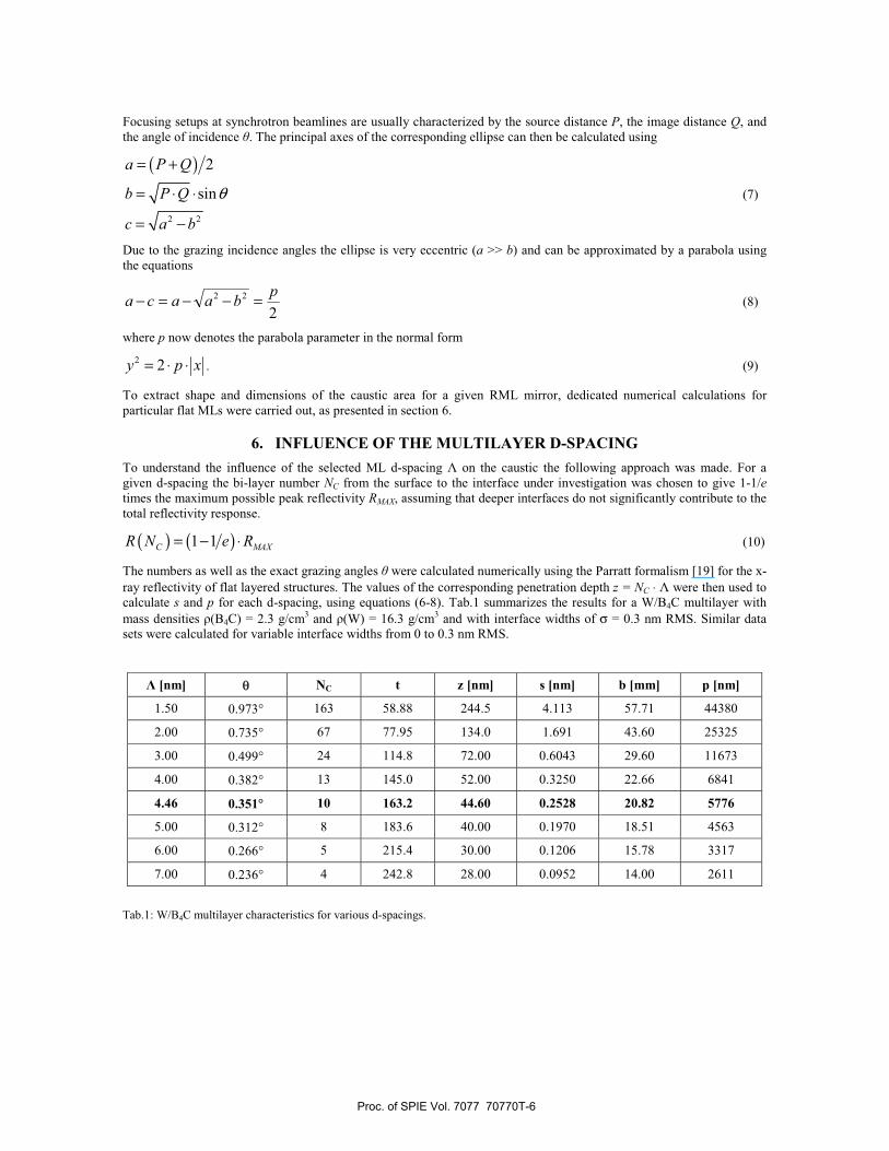
6. INFLUENCE OF THE MULTILAYER D-SPACING To understand the influence of the selected ML d-spacing � on the caustic the following approach was made. For a given d-spacing the bi-layer number NC from the surface to the interface under investigation was chosen to give 1-1/e times the maximum possible peak reflectivity RMAX, assuming that deeper interfaces do not significantly contribute to the total reflectivity response.

( ) ( )1 1C MAXR N e R= − ⋅ (10)

The numbers as well as the exact grazing angles � were calculated numerically using the Parratt formalism [19] for the x-ray reflectivity of flat layered structures. The values of the corresponding penetration depth z = NC ⋅ � were then used to calculate s and p for each d-spacing, using equations (6-8). Tab.1 summarizes the results for a W/B4C multilayer with mass densities �(B4C) = 2.3 g/cm3 and �(W) = 16.3 g/cm3 and with interface widths of σ = 0.3 nm RMS. Similar data sets were calculated for variable interface widths from 0 to 0.3 nm RMS.

� [nm] θ NC t z [nm] s [nm] b [mm] p [nm]

1.50 0.973° 163 58.88 244.5 4.113 57.71 44380

2.00 0.735° 67 77.95 134.0 1.691 43.60 25325

3.00 0.499° 24 114.8 72.00 0.6043 29.60 11673

4.00 0.382° 13 145.0 52.00 0.3250 22.66 6841

4.46 0.351° 10 163.2 44.60 0.2528 20.82 5776

5.00 0.312° 8 183.6 40.00 0.1970 18.51 4563

6.00 0.266° 5 215.4 30.00 0.1206 15.78 3317

7.00 0.236° 4 242.8 28.00 0.0952 14.00 2611

Tab.1: W/B4C multilayer characteristics for various d-spacings.

Proc. of SPIE Vol. 7077 70770T-6

7. CHROMATICITY Equations (3) offer the opportunity to estimate chromatic aberration in curved RMLs and to compare them with other types of focusing elements. The refractive decrement � is energy dependent. For hard x rays and far away from absorption edges it can be described by

21 Eδ � (11)

The change of the focal distance due to dispersive effects can be approximated by the first equation (3). Keeping the focusing geometry constant, it follows

20 0f f f f G E= + ∆ = + , (12)

where G varies only slowly with energy through s. The dispersion can therefore be written as

2RML

df fdE E

∆= ⋅ (13)

It is instructive to compare this result with the cases of FZPs and CRLs

FZP

df fdE E

= (14)

2CRL

df fdE E

= ⋅ (15)

The linear dependence of �f on δ may appear somewhat artificial and caused by the linear approximation on which the model is based. Indeed, higher order terms cannot be excluded, though occurring with very small coefficients. The essential point is, however, the fact that δ acts on �f and not on f.

To calculate the energy bandwidth that can be transmitted by an optical element at for given focusing geometry, one can demand that the chromatic blurring Dchrom must not exceed the diffraction limit Ddiff of the setup.

2 2 2 22tot diff chrom diffD D D D= + ≤ ⋅ (16)

The respective quantities are given by the following expressions

0.44diffD

NAλ⋅= (17)

2chromD NA df= ⋅ ⋅ (18)

for rectangular apertures, where NA is the numerical aperture of the optical element. Inserting expressions (17) and (18) in equation (16) one obtains

2 2

0.88 1.76diff totD Ddf

λ λ= =

⋅ ⋅ (19)

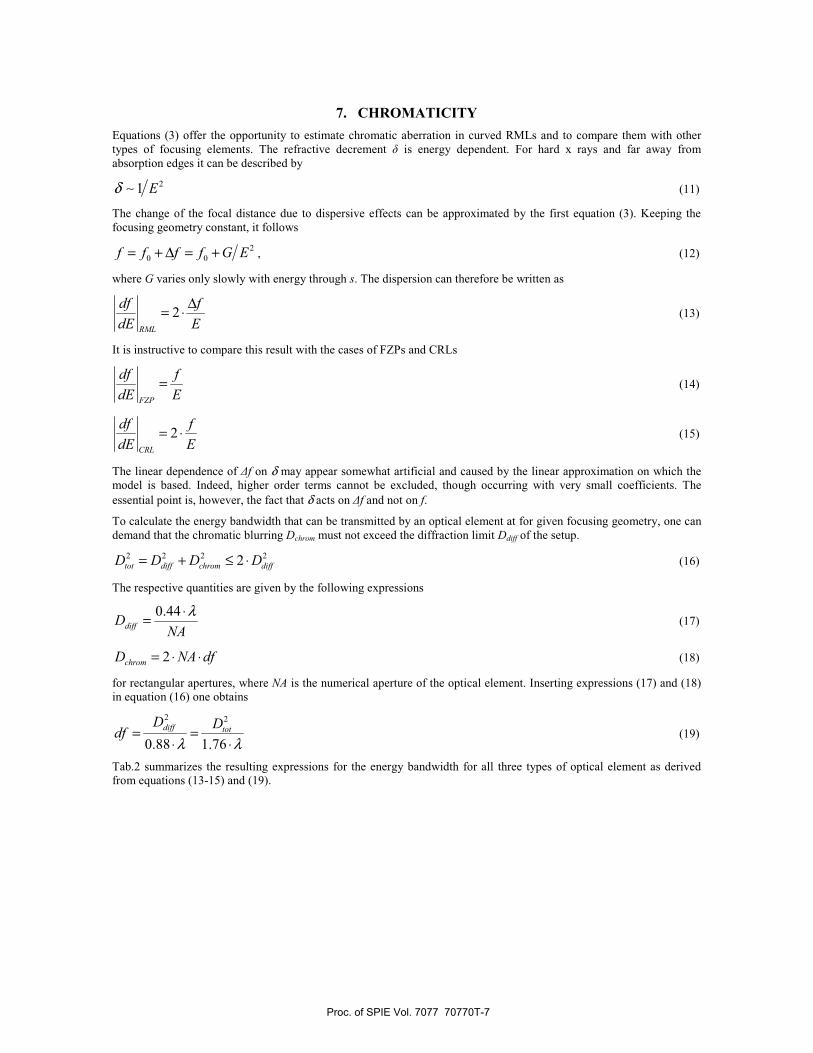
Tab.2 summarizes the resulting expressions for the energy bandwidth for all three types of optical element as derived from equations (13-15) and (19).

Proc. of SPIE Vol. 7077 70770T-7

FZP CRL RML

dEE

2

1.76totDf λ⋅ ⋅

2

3.52totDf λ⋅ ⋅

2

3.52totD

f λ⋅ ∆ ⋅

Tab.2: Comparison of the transmitted energy bandwidth of various optical elements.

The physical background of the different impact on the chromaticity is clearly visible. For FZPs and CRLs the phase shift induced by the optical elements is at the origin of their focusing properties and chromaticity therefore unavoidable. In the case of RMLs, however, it is rather a parasitic effect that should be suppressed as much as possible.

10-7

10-6

10-5

10-4

10-3

10-2

10-1

100

10-1 100 101 102 103

Tole

rate

d ba

ndpa

ss d

E/E

Total spot size Dtot

[nm]

f [mm]

1

10

100

Λ = 6nmMLs

CRLs

Mirrors

Undulator line

E = 20keV

Si(111)

FZPs

W/B4C MLs

Λ = 3nm

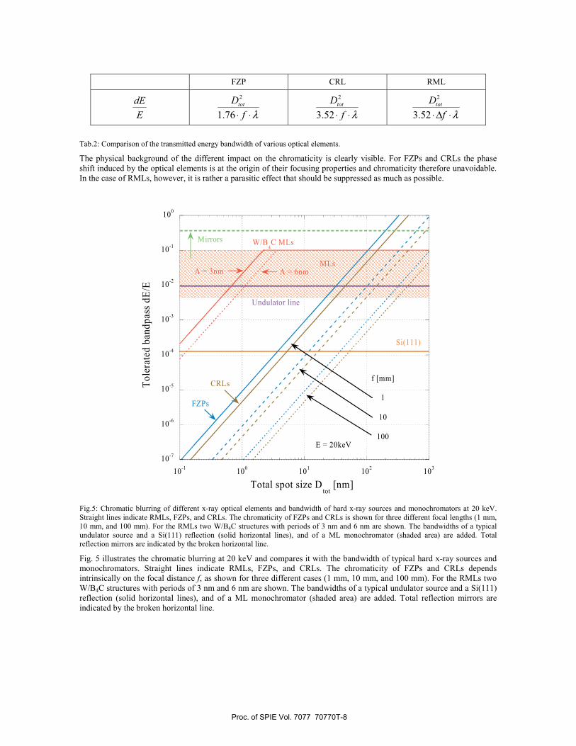
Fig.5: Chromatic blurring of different x-ray optical elements and bandwidth of hard x-ray sources and monochromators at 20 keV. Straight lines indicate RMLs, FZPs, and CRLs. The chromaticity of FZPs and CRLs is shown for three different focal lengths (1 mm, 10 mm, and 100 mm). For the RMLs two W/B4C structures with periods of 3 nm and 6 nm are shown. The bandwidths of a typical undulator source and a Si(111) reflection (solid horizontal lines), and of a ML monochromator (shaded area) are added. Total reflection mirrors are indicated by the broken horizontal line.

Fig. 5 illustrates the chromatic blurring at 20 keV and compares it with the bandwidth of typical hard x-ray sources and monochromators. Straight lines indicate RMLs, FZPs, and CRLs. The chromaticity of FZPs and CRLs depends intrinsically on the focal distance f, as shown for three different cases (1 mm, 10 mm, and 100 mm). For the RMLs two W/B4C structures with periods of 3 nm and 6 nm are shown. The bandwidths of a typical undulator source and a Si(111) reflection (solid horizontal lines), and of a ML monochromator (shaded area) are added. Total reflection mirrors are indicated by the broken horizontal line.

Proc. of SPIE Vol. 7077 70770T-8

Considering presently achievable focal spots sizes of about 100 nm, FZPs and CRLs can be operated with a Si(111) monochromator, for very short focal lengths (<10 mm) even with a full undulator line. RMLs are limited only by their intrinsic bandwidth of several percent. However, when going to focal spots of the order of 10 nm or below, declared aim of most 3rd generation synchrotron sources, FZPs and CRLs would require monochromators with an energy resolution better than 10-4, except for f < 10 mm. RMLs could still accept a full undulator line down to spots of less than 1 nm. The advantage would not only be higher photon flux on the sample. Scattering from nano-objects generally benefits from a broad energy bandpass.

Fig.5 does not describe the absolute focusing limit of the respective element, which is essentially given by equation (17). It complements the understanding by highlighting the influence of chromatic aberrations and helps to select the appropriate optical element for a given situation.

8. COMPARISON WITH EXPERIMENTAL DATA Focusing experiments were carried out on the ESRF insertion device beamline ID19, where a focal line with 45 nm FWHM was achieved [9]. A dynamically bent [W/B4C]25 ML mirror was used under the following conditions:

E = 24550 eV, λ = 0.05051 nm Λ = 4.457 nm � = 2.7 ⋅ 10-6

The ideal surface figure was assumed elliptic with the following values (with respect to the centre of the beam footprint on the mirror):

P = 150018.2 mm or equivalent a = 75047.5 mm Q = 76.9 mm b = 20.82 mm θ = 0.351° c = 75047.5 mm

The incident angle range along the beam footprint was � = 0.334°…0.371°.

This very eccentric ellipse can be approximated by a parabola using equation (8). The corresponding ML characteristics are given in Tab.1 (data row printed in bold).

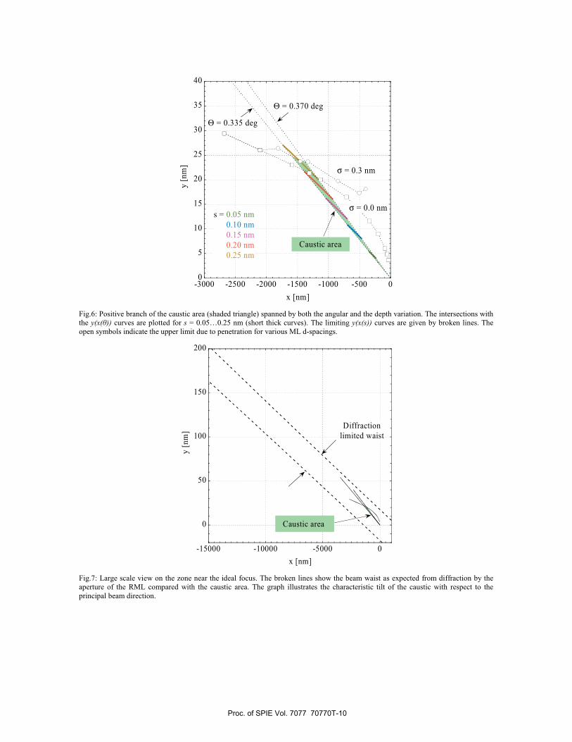
Based on the general interpretation in the previous section, the particular case of the ID19 experiment is illustrated in Fig.6. It shows the positive branch of the caustic area spanned by the angular variation along the RML combined with the depth variation of the reflecting interfaces. The upper limit is estimated by the penetration depth z (see Tab.1). It basically corresponds to a cone with its tip at the ideal focus that stretches up to values of x = -1.5 �m and y = 24 nm. The opening of the cone is limited to �y < 3 nm.

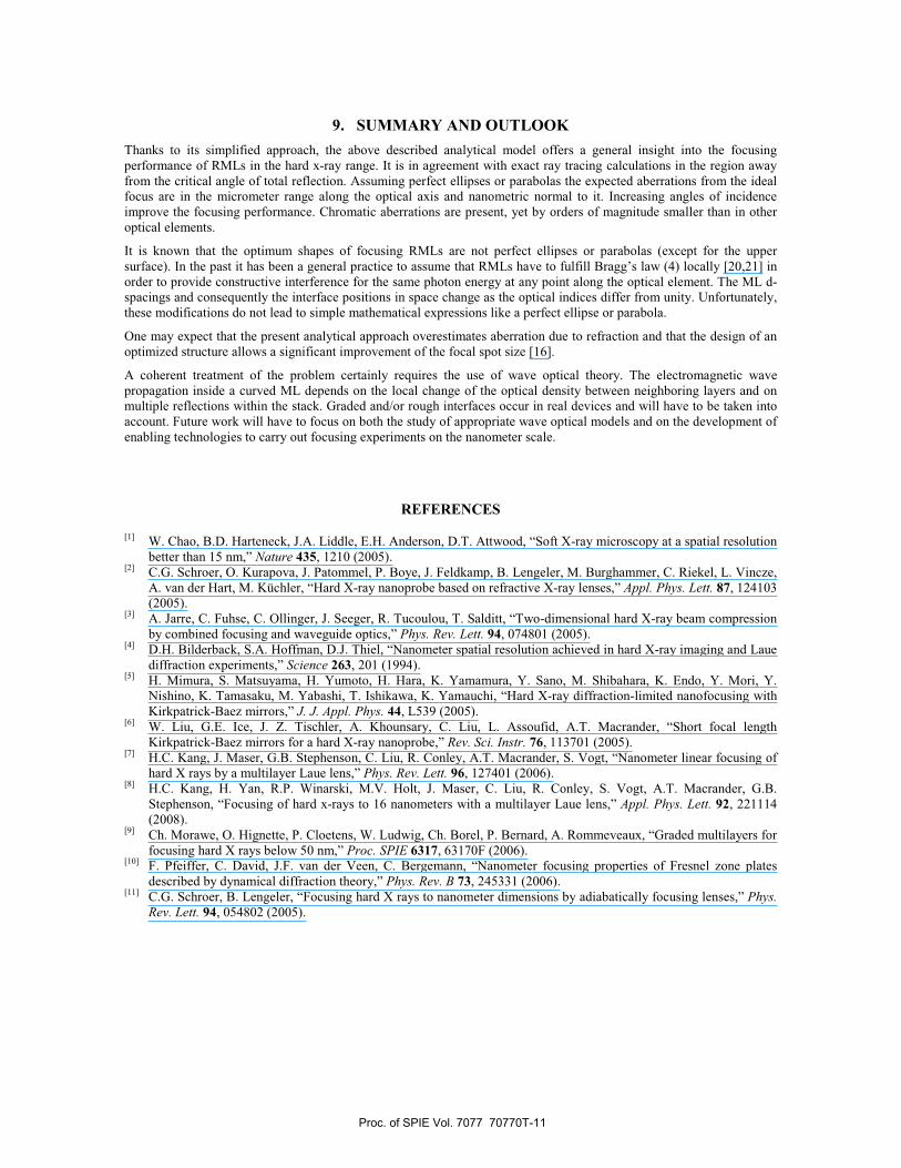
A comparison of the caustic area with the expected diffraction waist from the aperture of the RML is shown in Fig.7. In the present case, the diffraction limited spot size is about 35 nm FWHM. The measured size was 45 nm FWHM. It is evident that the spot size is dominated by diffraction effects and additional mirror imperfections. The figure also shows that the caustic is oriented almost parallel to the principal beam direction. Consequently, its impact on the spot size remains rather limited. If two symmetric RMLs facing each other were to be used, this advantage would disappear. In such a (rather ambitious) optical setup a significant reduction of the aberration effects would be mandatory to benefit from the improved numerical aperture.

It is evident from Fig.7 that the available experimental data is insufficient to confirm the presence of the caustic zone as derived within the analytical framework. RML based focusing optics with a diffraction limit below 10 nm would be needed. So far, such devices are not available, but strong efforts are under way to develop the required technologies [16].

Proc. of SPIE Vol. 7077 70770T-9

0

5

10

15

20

25

30

35

40

-3000 -2500 -2000 -1500 -1000 -500 0

y [n

m]

x [nm]

s = 0.05 nm0.10 nm0.15 nm0.20 nm0.25 nm

Θ = 0.370 deg

Θ = 0.335 deg

σ = 0.0 nm

σ = 0.3 nm

Caustic area

Fig.6: Positive branch of the caustic area (shaded triangle) spanned by both the angular and the depth variation. The intersections with the y(x(�)) curves are plotted for s = 0.05…0.25 nm (short thick curves). The limiting y(x(s)) curves are given by broken lines. The open symbols indicate the upper limit due to penetration for various ML d-spacings.

0

50

100

150

200

-15000 -10000 -5000 0

y [n

m]

x [nm]

Diffractionlimited waist

Caustic area

Fig.7: Large scale view on the zone near the ideal focus. The broken lines show the beam waist as expected from diffraction by the aperture of the RML compared with the caustic area. The graph illustrates the characteristic tilt of the caustic with respect to the principal beam direction.

Proc. of SPIE Vol. 7077 70770T-10

9. SUMMARY AND OUTLOOK Thanks to its simplified approach, the above described analytical model offers a general insight into the focusing performance of RMLs in the hard x-ray range. It is in agreement with exact ray tracing calculations in the region away from the critical angle of total reflection. Assuming perfect ellipses or parabolas the expected aberrations from the ideal focus are in the micrometer range along the optical axis and nanometric normal to it. Increasing angles of incidence improve the focusing performance. Chromatic aberrations are present, yet by orders of magnitude smaller than in other optical elements.

It is known that the optimum shapes of focusing RMLs are not perfect ellipses or parabolas (except for the upper surface). In the past it has been a general practice to assume that RMLs have to fulfill Bragg’s law (4) locally [20,21] in order to provide constructive interference for the same photon energy at any point along the optical element. The ML d-spacings and consequently the interface positions in space change as the optical indices differ from unity. Unfortunately, these modifications do not lead to simple mathematical expressions like a perfect ellipse or parabola.

One may expect that the present analytical approach overestimates aberration due to refraction and that the design of an optimized structure allows a significant improvement of the focal spot size [16].

A coherent treatment of the problem certainly requires the use of wave optical theory. The electromagnetic wave propagation inside a curved ML depends on the local change of the optical density between neighboring layers and on multiple reflections within the stack. Graded and/or rough interfaces occur in real devices and will have to be taken into account. Future work will have to focus on both the study of appropriate wave optical models and on the development of enabling technologies to carry out focusing experiments on the nanometer scale.

REFERENCES

[1] W. Chao, B.D. Harteneck, J.A. Liddle, E.H. Anderson, D.T. Attwood, “Soft X-ray microscopy at a spatial resolution better than 15 nm,” Nature 435, 1210 (2005).

[2] C.G. Schroer, O. Kurapova, J. Patommel, P. Boye, J. Feldkamp, B. Lengeler, M. Burghammer, C. Riekel, L. Vincze, A. van der Hart, M. Küchler, “Hard X-ray nanoprobe based on refractive X-ray lenses,” Appl. Phys. Lett. 87, 124103 (2005).

[3] A. Jarre, C. Fuhse, C. Ollinger, J. Seeger, R. Tucoulou, T. Salditt, “Two-dimensional hard X-ray beam compression by combined focusing and waveguide optics,” Phys. Rev. Lett. 94, 074801 (2005).

[4] D.H. Bilderback, S.A. Hoffman, D.J. Thiel, “Nanometer spatial resolution achieved in hard X-ray imaging and Laue diffraction experiments,” Science 263, 201 (1994).

[5] H. Mimura, S. Matsuyama, H. Yumoto, H. Hara, K. Yamamura, Y. Sano, M. Shibahara, K. Endo, Y. Mori, Y. Nishino, K. Tamasaku, M. Yabashi, T. Ishikawa, K. Yamauchi, “Hard X-ray diffraction-limited nanofocusing with Kirkpatrick-Baez mirrors,” J. J. Appl. Phys. 44, L539 (2005).

[6] W. Liu, G.E. Ice, J. Z. Tischler, A. Khounsary, C. Liu, L. Assoufid, A.T. Macrander, “Short focal length Kirkpatrick-Baez mirrors for a hard X-ray nanoprobe,” Rev. Sci. Instr. 76, 113701 (2005).

[7] H.C. Kang, J. Maser, G.B. Stephenson, C. Liu, R. Conley, A.T. Macrander, S. Vogt, “Nanometer linear focusing of hard X rays by a multilayer Laue lens,” Phys. Rev. Lett. 96, 127401 (2006).

[8] H.C. Kang, H. Yan, R.P. Winarski, M.V. Holt, J. Maser, C. Liu, R. Conley, S. Vogt, A.T. Macrander, G.B. Stephenson, “Focusing of hard x-rays to 16 nanometers with a multilayer Laue lens,” Appl. Phys. Lett. 92, 221114 (2008).

[9] Ch. Morawe, O. Hignette, P. Cloetens, W. Ludwig, Ch. Borel, P. Bernard, A. Rommeveaux, “Graded multilayers for focusing hard X rays below 50 nm,” Proc. SPIE 6317, 63170F (2006).

[10] F. Pfeiffer, C. David, J.F. van der Veen, C. Bergemann, “Nanometer focusing properties of Fresnel zone plates described by dynamical diffraction theory,” Phys. Rev. B 73, 245331 (2006).

[11] C.G. Schroer, B. Lengeler, “Focusing hard X rays to nanometer dimensions by adiabatically focusing lenses,” Phys. Rev. Lett. 94, 054802 (2005).

Proc. of SPIE Vol. 7077 70770T-11

[12] K. Yamauchi, K. Yamamura, H. Mimura, Y. Sano, A. Saito, A. Souvorov, M. Yabashi, K. Tamasaku, T. Ishikawa, Y. Mori, “Nearly diffraction-limited line focusing of hard X-ray beam with an elliptically figured mirror,” J. Synchrotron Rad. 9, 313 (2002).

[13] C.M. Kewish, L. Assoufid, A.T. Macrander, J. Qian, “Wave-optical simulation of hard X-ray nanofocusing by precisely figured elliptical mirrors,” Appl. Optics 46, 2010 (2007).

[14] C.G. Schroer, “Focusing hard X rays to nanometer dimensions using Fresnel zone plates,” Phys. Rev. B 74, 033405 (2006).

[15] H. Yan, J. Maser, A.T. Macrander, Q. Shen, S. Vogt, G.B. Stephenson, H.C. Kang, “Takagi-Taupin description of X-ray dynamical diffraction from diffractive optics with large numerical aperture,” Phys. Rev. B 76, 115438 (2007).

[16] H. Mimura, S. Matsuyama, H. Yumoto, S. Handa, T. Kimura, Y. Sano, K. Tamasaku, Y. Nishino, M. Yabashi, T. Ishikawa, K. Yamauchi, “Reflective optics for sub-10nm hard X-ray focusing,” Proc. SPIE 6705, 67050L (2007).

[17] J-P. Guigay, Ch. Morawe, V. Mocella, C. Ferrero, “An analytical approach to estimating aberrations in curved multilayer optics for hard x-rays: 1. Derivation of caustic shapes,” Opt. Express 16, 12050 (2008).

[18] Ch. Morawe, J-P. Guigay, V. Mocella, C. Ferrero, “An analytical approach to estimating aberrations in curved multilayer optics for hard x-rays: 2. Interpretation and application to focusing experiments,” Opt. Express (submitted)

[19] L.G. Parratt, “Surface studies of solids by total reflection of x-rays,” Phys. Rev. 45, 359 (1954). [20] M. Schuster, H. Göbel, “Parallel beam coupling into channel-cut monochromators using curved graded multilayers”,

J. Phys. D: Appl. Phys., 28, A270 (1995). [21] Ch. Morawe, P. Pecci, J-Ch. Peffen, E. Ziegler, ”Design and performance of graded multilayers as focusing

elements for x-ray optics,” Rev. Sci. Instr. 70, 3227 (1999).

Proc. of SPIE Vol. 7077 70770T-12