Embed Size (px)
Citation preview
Multi-scale representation of differential profiles for high-throughput biomarker datasets 1
Abstract
High-throughput screening (HTS) is a set of measurement techniques relevant in the fields of
biology, chemistry and medicine. Since the publication of the human genome project, HTS has
become a key technology allowing a researcher to quickly conduct millions of chemical, genetic
and pharmacological tests. Results obtained from these tests are usually represented in form of
networks and similar type of diagrams in order to facilitate biological interpretation. However, it is
difficult to find tools which display and manage the massive number of biomarkers involved without
crashing, requiring a lot of computer memory and showing a complex framework to understand
and use.
Therefore, this project specifies, designs and builds methods for the representation of large
datasets from high throughput screening, concretely metabolomics and Gas Chromatography -
Mass Spectrometry (GC-MS). The methodology is based on applying clustering algorithms to
these datasets to visualize the networks they form at different scales. It uses external information
from databases such as KEGG Pathways, Reactome and the Human Metabolome Database in
order to include curated information of signalling pathways and reactions in human biology.
Finally, a lightweight application is developed in order to display and manipulate both small and
large networks, for the latter applying the mentioned methods. This program also includes extra
functionalities which have been requested and specified by potential users through interviews.

2 Multi-scale representation of differential profiles for high-throughput biomarker datasets
Multi-scale representation of differential profiles for high-throughput biomarker datasets 3
Contents
Abstract ......................................................................................................................................... 1
Contents ........................................................................................................................................ 3
List of Figures ............................................................................................................................... 5
1. Introduction ............................................................................................................................... 7
1.1. Motivation ............................................................................................................................. 7
1.2. Objectives ............................................................................................................................ 7
1.3. Reaching .............................................................................................................................. 8
2. Context ...................................................................................................................................... 9
2.1. Kyoto Encyclopedia of Genes and Genomes (KEGG) .......................................................... 9
2.2. Reactome Pathway Database ............................................................................................ 10
2.3. The Human Metabolome Database (HMDB) ...................................................................... 12
2.4. Metabolomics ..................................................................................................................... 12
2.5. Transcriptomics .................................................................................................................. 13
2.6. The Gene Ontology (GO) ................................................................................................... 14
2.7. RStudio and Bioconductor .................................................................................................. 14
3. State of the art ......................................................................................................................... 16
4. Programming language .......................................................................................................... 20
4.1. Alternatives ........................................................................................................................ 20
4.2. Data-Driven Documents (D3.js) and JavaScript ................................................................. 21
4.3. Prototype building .............................................................................................................. 23
5. Specific requirements ............................................................................................................. 25
5.1. Interview 1 .......................................................................................................................... 25
5.2. Interview 2 .......................................................................................................................... 26
5.3. Interview 3 .......................................................................................................................... 28
5.4. Requirements' summarize .................................................................................................. 29
6. Design and development of the application .......................................................................... 31
6.1. Appearance and operation ................................................................................................. 31
6.1.1. Visualization controllers ............................................................................................... 31
6.1.2. Graph display .............................................................................................................. 35
6.1.3. Extended controllers .................................................................................................... 39
6.2. Creation of .json files .......................................................................................................... 43
7. Large networks ....................................................................................................................... 45
7.1. Graph clustering methods .................................................................................................. 45
7.1.1. Spectral clustering ....................................................................................................... 48
7.2. Application of spectral clustering to a big network .............................................................. 51
7.3. Creation of .json files .......................................................................................................... 52
4 Multi-scale representation of differential profiles for high-throughput biomarker datasets
7.4. Visualization of clusters ...................................................................................................... 54
8. Integration with R .................................................................................................................... 57
9. Economic estimation and planning ....................................................................................... 58
9.1. Economic estimation .......................................................................................................... 58
9.2. Planning ............................................................................................................................. 58
10. Environmental impact ........................................................................................................... 60
Conclusions and further work ................................................................................................... 61
Bibliography ................................................................................................................................ 62
A. Interviews ................................................................................................................................ 64
A.1. Interview 1 ......................................................................................................................... 64
A2. Interview 2 .......................................................................................................................... 65
A.3. Interview 3 ......................................................................................................................... 66
B. BIMS Viewer’s full code ......................................................................................................... 68
B.1. index.html .......................................................................................................................... 68
B.2. index2.html ........................................................................................................................ 74
B.3. plot.js ................................................................................................................................. 79
B.4. CreateJSON.R ................................................................................................................. 116
B.5. SpectralClustering.R ........................................................................................................ 133
C. Dijkstra algorithm ................................................................................................................. 137
Multi-scale representation of differential profiles for high-throughput biomarker datasets 5
List of Figures
Fig 2.1: KEGG representation of Cysteine and Methionine metabolism. ....................................... 10
Fig 2.2: Reactome representation of Homo Sapiens pathways and their connections. .................. 11
Fig 2.3: Number of entries of all species contained in Reactome. ................................................. 11
Fig 2.4: GC-MS diagram and GC-MS spectrum. ........................................................................... 13
Fig 2.5: Microarray instruments and signal generated by a microarray. ......................................... 13
Fig 3.1: Example of a network visualized with Cytoscape and with IPA. ........................................ 16
Fig 3.2: Example of one of PHINCH representations and one of BioLayout representations. ........ 17
Fig 3.3: Example of a network visualized with Osprey and with Omix. .......................................... 18
Fig 3.4: Table comparing different programs which display biological data ................................... 18
Fig 4.1: Changing the color of a paragraph using selections. ........................................................ 21
Fig 4.2: Two ways of applying color to several elements with D3.. ................................................ 22
Fig 4.3: Prototype which was shown to all interviewees.. .............................................................. 23
Fig 4.4: Structure of prototype’s code.. .......................................................................................... 24
Fig 5.1: Shiny application developed by the interviewee.. ............................................................. 26
Fig 5.2: Example of a representation using enrichMap function and cnetplot. ............................... 27
Fig 5.3: Example of sunburst, hypertree and treemap. .................................................................. 28
Fig 5.4: Example of a MetScape representation. ........................................................................... 29
Fig 6.1: Welcome screen of BiMS. ................................................................................................ 32
Fig 6.2: Diagram showing the operation of the welcome screen’s buttons.. ................................... 33
Fig 6.3: Code which creates the visualization controllers’ buttons and their functionalities. ........... 34
Fig 6.4: Demonstration of Create Network button’s functionality.. ................................................. 35
Fig 6.5: First commands of viewNetwork function. ........................................................................ 36
Fig 6.6: Creation of visualization area rectangle. ........................................................................... 36
Fig 6.7: Implementation of zoom properties. ................................................................................. 36
Fig 6.8: Addition of extended controllers to the bottom row of buttons. .......................................... 37
Fig 6.9: Setting of nodes’ attributes. .............................................................................................. 38
Fig 6.10: json file with nodes’ and links’ properties. ....................................................................... 38
Fig 6.11: Show/Hide Labels button’s functionality demonstration. ................................................. 39
Fig 6.12: Search Node button’s functionality demonstration.. ........................................................ 40
Fig 6.13: Show Path button’s functionality demonstration. ............................................................ 40
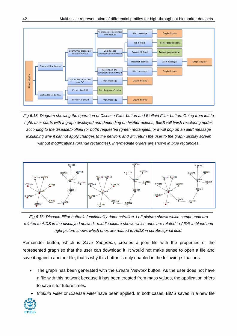
Fig 6.14: Disease Filter’s response when there is more than one disease containing the word
written by the user. ........................................................................................................................ 41
Fig 6.15: Diagram showing the operation of Disease Filter button and Biofluid Filter button.. ........ 42
Fig 6.16: Disease Filter button’s functionality demonstration.. ....................................................... 42
6 Multi-scale representation of differential profiles for high-throughput biomarker datasets
Fig 7.1: K-means operation.. ......................................................................................................... 46
Fig 7.2: Hierarchical clustering (agglomerative) and DBSCAN operation.. .................................... 46
Fig 7.3: Comparison of results given by K-means, hierarchical clustering, spectral clustering and
DBSCAN on different sets of points. ............................................................................................. 47
Fig 7.4: Comparison of results applying different combinations of similarity graphs and Laplacians
in spectral clustering, given a set of points. ................................................................................... 49
Fig 7.5: Table studying parameter adjustment in spectral clustering. ............................................ 50
Fig 7.6: Data frame containing spectral clustering results on the compounds graph.. ................... 52
Fig 7.7: Network with 100 nodes and lots of links with its places decided by the application. ........ 52
Fig 7.8: Nodes’ location before and after applying the algorithm to place all nodes from the same
cluster together. ............................................................................................................................ 53
Fig 7.9: Paint Clusters button’s functionality demonstration. ......................................................... 56
Fig 9.1: Table showing the economic estimation of the project. ..................................................... 58
Fig 9.2: Gant diagram of the project.. ............................................................................................ 59
Multi-scale representation of differential profiles for high-throughput biomarker datasets 7
1. Introduction
1.1. Motivation
The motivation for this project is to create a useful tool for the Bioinformatics and Biomedical
Signals Laboratory (B2SLab). Researchers usually need to represent large datasets (these
obtained, for example, after performing enrichments on metabolomic experiments), in order to infer
biological interpretation from them. This task would be easier with a lightweight and interactive
visualization tool, especially if it could be combined with the statistical programs they use, and this
will be developed during this project.
As the application is meant to give as much service as possible, requirements will be set up after
three interviews to different profiles of professionals, all of them researchers or collaborators of the
B2SLab: a researcher in bioinformatics, a researcher in biomedical datum analysis and a
biochemist. They will be shown a little demonstration of how the tool will work through a simple
prototype in order to make them easier to describe what they need in a final product. Therefore,
the application will be developed by following these steps:
Design of a prototype.
Set up of requirements through interviews.
Building of final application.
1.2. Objectives
The purpose of this project is to develop a lightweight application with the following main
objectives:
Displaying networks and manipulating them.
Implementing a multi-scale feature which also allows representing large graphs.
Building methods to cluster nodes in order to achieve the previous goal.
Allowing integration into statistical analyses tools.
Design oriented towards metabolomics and gas chromatography - mass spectrometry (GC-
MS).

8 Multi-scale representation of differential profiles for high-throughput biomarker datasets
1.3. Reaching
Regarding to the application itself, the reaching of this project will cover the design, development
and building of the application, but not its launching to the market.
Multi-scale representation of differential profiles for high-throughput biomarker datasets 9
2. Context
It has been mentioned before that the application designed in this project uses external information
from databases such as KEGG Pathways, Reactome and the Human Metabolome Database, that
it is oriented towards metabolomics and transcriptomics and that it should be integrated into
statistical analyses tools. All these concepts are important to understand the development of the
project and are introduced within this chapter.
2.1. Kyoto Encyclopedia of Genes and Genomes (KEGG)
KEGG [1] is a database resource for understanding high-level functions and utilities of the
biological system, such as the cell, the organism and the ecosystem, from molecular-level
information, especially large-scale molecular datasets generated by genome sequencing and other
high-throughput experimental technologies.
This database contains various data objects for computer representation of the biological systems,
each one assigned a KEGG identification. The ones of interest of this project and their respective
number of entries (in brackets) are:
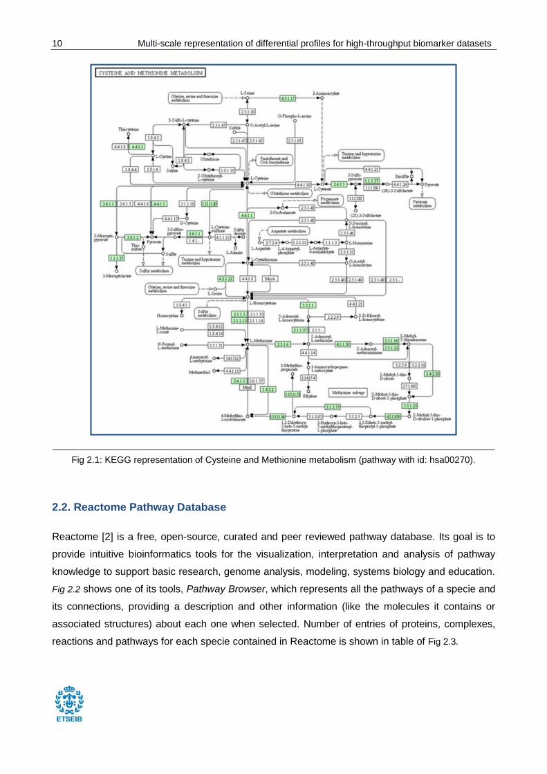
Pathways (474): wiring diagrams of molecular interactions, reactions, and relations (see Fig
2.1).
Modules (706): functional units used for annotation and interpretation of sequenced
genomes.
Enzymes (6.510): macromolecular biological catalysts.
Reactions (9.884): knowledge base for predicting biodegradation and biosynthesis.
Compounds (17.419): small molecules, biopolymers, and other chemical substances which
are relevant to biological systems.
10 Multi-scale representation of differential profiles for high-throughput biomarker datasets
____________________________________________________________________________________________________________
Fig 2.1: KEGG representation of Cysteine and Methionine metabolism (pathway with id: hsa00270).
2.2. Reactome Pathway Database
Reactome [2] is a free, open-source, curated and peer reviewed pathway database. Its goal is to
provide intuitive bioinformatics tools for the visualization, interpretation and analysis of pathway
knowledge to support basic research, genome analysis, modeling, systems biology and education.
Fig 2.2 shows one of its tools, Pathway Browser, which represents all the pathways of a specie and
its connections, providing a description and other information (like the molecules it contains or
associated structures) about each one when selected. Number of entries of proteins, complexes,
reactions and pathways for each specie contained in Reactome is shown in table of Fig 2.3.

Multi-scale representation of differential profiles for high-throughput biomarker datasets 11
____________________________________________________________________________________________________________
Fig 2.2: Reactome representation of Homo Sapiens pathways and their connections.
SPECIES PROTEINS COMPLEXES REACTIONS PATHWAYS
D. discoideum 1668 1387 1435 826
P. falciparum 622 514 500 447
S. pombe 1149 1039 1016 678
S. cerevisiae 1271 1039 1092 689
C. elegans 3943 2572 2510 1044
S. scrofa 8521 5958 5642 1389
B. taurus 8000 6565 6240 1421
C. familiaris 8394 6411 6059 1411
M. musculus 8891 7030 6639 1451
R. norvegicus 8832 6702 6364 1423
*H. sapiens 7951 7895 8169 1762
G. gallus 5835 5580 5172 1442
T. guttata 5846 5016 4685 1347
X. tropicalis 7869 5826 5566 1387
D. rerio 11720 5817 5547 1386
D. melanogaster 6973 3131 3114 1148
A. thaliana 4056 1278 1342 764
O. sativa 4999 1291 1375 774
M. tuberculosis 13 58 40 12
___________________________________________________________________________________________________________
Fig 2.3: Number of proteins’, complexes’, reactions’ and pathways’ entries of all species contained in Reactome.
12 Multi-scale representation of differential profiles for high-throughput biomarker datasets
2.3. The Human Metabolome Database (HMDB)
The Human Metabolome Database (HMDB) [3] is a freely available electronic database containing
detailed information about small molecule metabolites found in the human body. It is intended to be
used for applications in metabolomics, clinical chemistry, biomarker discovery and general
education. The database is designed to contain or link three kinds of data:
chemical data
clinical data
molecular biology/biochemistry data
The database contains 41,993 metabolite entries including both water-soluble and lipid soluble
metabolites as well as metabolites that would be regarded as either abundant (> 1 uM) or relatively
rare (< 1 nM). Additionally, 5,688 protein sequences are linked to these metabolite entries. Each
MetaboCard entry contains more than 110 data fields with 2/3 of the information being devoted to
chemical/clinical data and the other 1/3 devoted to enzymatic or biochemical data. Many data fields
are hyperlinked to other databases (KEGG, PubChem, MetaCyc, ChEBI, PDB, UniProt, and
GenBank) and a variety of structure and pathway viewing applets.
2.4. Metabolomics
Metabolomics [4] is the scientific study of chemical processes involving metabolites, which are
small molecules product of the metabolism. Metabolites have different functions, like fuel,
structure, stimulatory and inhibitory effects on enzymes, catalytic activity of their own, defense and
interactions with other organisms.
There are different ways of performing metabolomics and they divide in separation, ionization and
detection methods. Concretely, the ones of interest of this project are the followings:
Gas chromatography (GC): it is a separation method consisting of separating and analyzing
compounds that can be vaporized without decomposition. It is one of the most widely used
methods for metabolomic analysis, especially when combined with mass spectrometry
(GC-MS).
Mass spectrometry (MS): it is a detection method used to identify and quantify metabolites
after optional separation by GC or other technologies.
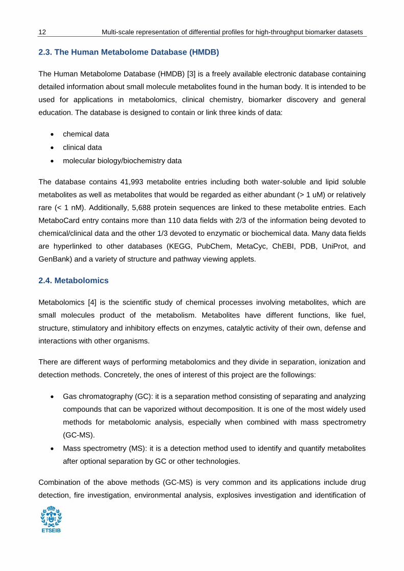
Combination of the above methods (GC-MS) is very common and its applications include drug
detection, fire investigation, environmental analysis, explosives investigation and identification of
Multi-scale representation of differential profiles for high-throughput biomarker datasets 13
unknown samples. Fig 2.4 shows a diagram of GC-MS operation and result.
___________________________________________________________________________________________________________
Fig 2.4: GC-MS diagram (left) and GC-MS spectrum (right).
2.5. Transcriptomics
Transcriptomics is the study of the transcriptome—the complete set of RNA transcripts that are
produced by the genome, under specific circumstances or in a specific cell—using high-throughput
methods, such as microarray analysis. Comparison of transcriptomes allows the identification of
genes that are differentially expressed in distinct cell populations, or in response to different
treatments.
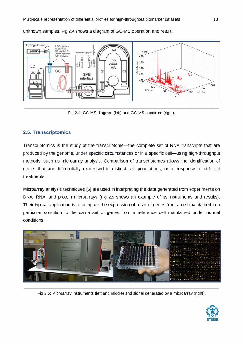
Microarray analysis techniques [5] are used in interpreting the data generated from experiments on
DNA, RNA, and protein microarrays (Fig 2.5 shows an example of its instruments and results).
Their typical application is to compare the expression of a set of genes from a cell maintained in a
particular condition to the same set of genes from a reference cell maintained under normal
conditions.
___________________________________________________________________________________________________________
Fig 2.5: Microarray instruments (left and middle) and signal generated by a microarray (right).
14 Multi-scale representation of differential profiles for high-throughput biomarker datasets
2.6. The Gene Ontology (GO)
Information about genes can be found in the Gene Ontology (GO), a major bioinformatics initiative
to unify the representation of gene and gene product attributes across all species [6]. Founded in
1998, the project began as a collaboration between three model organism databases, FlyBase
(Drosophila), the Saccharomyces Genome Database (SGD) and the Mouse Genome Database
(MGD). The GO Consortium (GOC) has since grown to incorporate many databases, including
several of the world's major repositories for plant, animal, and microbial genomes.
It has developed three structured ontologies that describe gene products in terms of their
associated biological processes, cellular components and molecular functions in a species-
independent manner. These are very interesting in transcriptomics and required at the time of
visualizing results.
Biological Processes (BP): describe series of events accomplished by one or more
organized assemblies of molecular functions. These can be broad terms (for example,
"cellular physiological process" or "signal transduction") or more specific terms (like
"pyrimidine metabolic process" or "alpha-glucoside transport").
Cellular Components (CC): describe components of a cell that are part of larger objects,
such as an anatomical structure (for example, “rough endoplasmic reticulum” or “nucleus”)
or a gene product group (like “ribosome” or “proteasome”).
Molecular Functions (MF): describe activities that occur at the molecular level, such as
"catalytic activity" or "binding activity".
The general rule to assist in distinguishing between a biological process and a molecular function
is that a process must have more than one distinct steps.
2.7. RStudio and Bioconductor
RStudio [7] is a free and open source integrated development environment (IDE) with a powerful
and productive user interface for R, which is a free software environment for statistical computing
and graphics that compiles and runs on a wide variety of UNIX platforms, Windows and MacOS.
Apart from its inner functionalities, RStudio provides lots of extra ones by installing different
packages and it is widely used for statistical data analysis.
Multi-scale representation of differential profiles for high-throughput biomarker datasets 15
Bioconductor [8] is an open source and open development software project to provide tools for the
analysis and comprehension of high-throughput genomic data. It is based primarily on the R
programming language and most of its components are distributed as R packages. The functional
of Bioconductor packages includes the analysis of DNA microarray, sequence and other data, that
is why Rstudio is a very used tool for bioinformatics analysis. These packages are divided in three
groups:
Software: 1.024 packages which are classified, at the same time, in the following groups
according to the analytic calculations they allow performing: Assay Domain, Biological
Question, Infrastructure, Research Field, Statistical Method, Technology and Workflow
Step.
Annotation: 883 database-like packages that provide information linking identifiers (for
example, Entrez gene names or Affymetrix probe ids) to other information (like
chromosomal location, Gene Ontology category).
Experiment: data packages which provide data sets that are used, often by software
packages, to illustrate particular analyses.
Developers often provide or use an existing experiment data package to give a comprehensive
illustration of the methods in the software package.
16 Multi-scale representation of differential profiles for high-throughput biomarker datasets
3. State of the art
The present day, there are lots of good visualization programs focused on displaying biological
data, and they are continuously updating at the same time that new ones appear, all of them to
cover new necessities. So, before starting the design of the application, a market research has
been made in order to see the tendencies they follow and extract conclusions to the current
project. Six software packages have been selected as a sample and, after a short description of
each one, table in Fig 3.4compares its main characteristics.
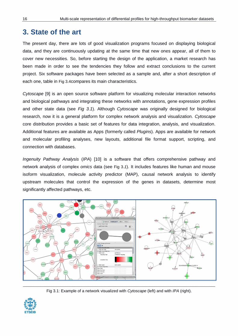
Cytoscape [9] is an open source software platform for visualizing molecular interaction networks
and biological pathways and integrating these networks with annotations, gene expression profiles
and other state data (see Fig 3.1). Although Cytoscape was originally designed for biological
research, now it is a general platform for complex network analysis and visualization. Cytoscape
core distribution provides a basic set of features for data integration, analysis, and visualization.
Additional features are available as Apps (formerly called Plugins). Apps are available for network
and molecular profiling analyses, new layouts, additional file format support, scripting, and
connection with databases.
Ingenuity Pathway Analysis (IPA) [10] is a software that offers comprehensive pathway and
network analysis of complex omics data (see Fig 3.1). It includes features like human and mouse
isoform visualization, molecule activity predictor (MAP), causal network analysis to identify
upstream molecules that control the expression of the genes in datasets, determine most
significantly affected pathways, etc.
____________________________________________________________________________________________________________
Fig 3.1: Example of a network visualized with Cytoscape (left) and with IPA (right).
Multi-scale representation of differential profiles for high-throughput biomarker datasets 17
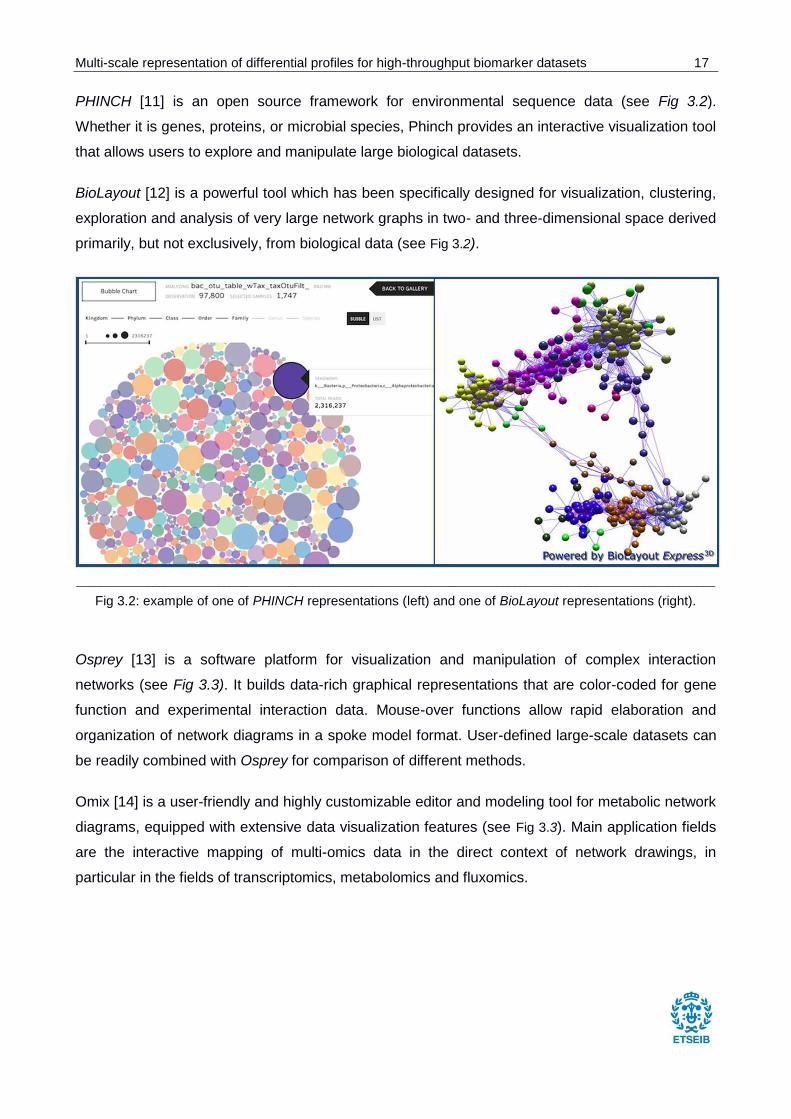
PHINCH [11] is an open source framework for environmental sequence data (see Fig 3.2).
Whether it is genes, proteins, or microbial species, Phinch provides an interactive visualization tool
that allows users to explore and manipulate large biological datasets.
BioLayout [12] is a powerful tool which has been specifically designed for visualization, clustering,
exploration and analysis of very large network graphs in two- and three-dimensional space derived
primarily, but not exclusively, from biological data (see Fig 3.2).
____________________________________________________________________________________________________________
Fig 3.2: example of one of PHINCH representations (left) and one of BioLayout representations (right).
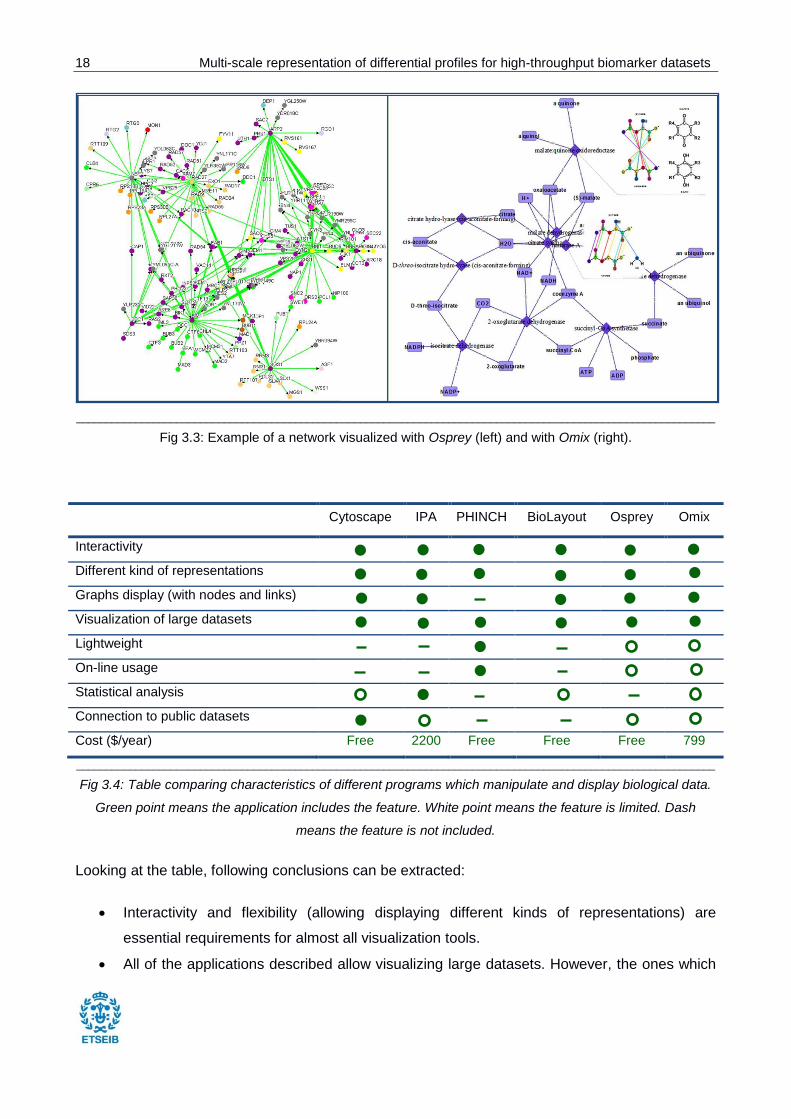
Osprey [13] is a software platform for visualization and manipulation of complex interaction
networks (see Fig 3.3). It builds data-rich graphical representations that are color-coded for gene
function and experimental interaction data. Mouse-over functions allow rapid elaboration and
organization of network diagrams in a spoke model format. User-defined large-scale datasets can
be readily combined with Osprey for comparison of different methods.
Omix [14] is a user-friendly and highly customizable editor and modeling tool for metabolic network
diagrams, equipped with extensive data visualization features (see Fig 3.3). Main application fields
are the interactive mapping of multi-omics data in the direct context of network drawings, in
particular in the fields of transcriptomics, metabolomics and fluxomics.
18 Multi-scale representation of differential profiles for high-throughput biomarker datasets
____________________________________________________________________________________________________________
Fig 3.3: Example of a network visualized with Osprey (left) and with Omix (right).
Cytoscape IPA PHINCH BioLayout Osprey Omix
Interactivity
Different kind of representations
Graphs display (with nodes and links)
Visualization of large datasets
Lightweight
On-line usage
Statistical analysis
Connection to public datasets
Cost ($/year) Free 2200 Free Free Free 799
____________________________________________________________________________________________________________
Fig 3.4: Table comparing characteristics of different programs which manipulate and display biological data.
Green point means the application includes the feature. White point means the feature is limited. Dash
means the feature is not included.
Looking at the table, following conclusions can be extracted:
Interactivity and flexibility (allowing displaying different kinds of representations) are
essential requirements for almost all visualization tools.
All of the applications described allow visualizing large datasets. However, the ones which
Multi-scale representation of differential profiles for high-throughput biomarker datasets 19
require installation (no on-line usage) request for a 2GB minimum space in the user's
computer to use this feature. Unfortunately, the other program, which is capable of
representing large datasets (PHINCH), does not represent networks but other graphics.
Visualization and statistical analysis usually go together in many programs. However, the
latter is often less developed and focused only in gene enrichment analysis.
There are really good visualization tools both free and commercial.
At present day, there are lots of public databases related to different biomedical areas (for
example, KEGG, Reactome or GO) from which applications extract information in order to
make easier researchers' analysis. This is a quite interesting feature to have and that is
why most of the programs described are progressively connecting to more datasets.
In the light of the above, it would be very useful to have a new application which, apart from the
essential interactivity feature, it focused on:
Optimization in visualizing large datasets in form of graphs (in terms of memory
requirements in the computer). It is for this purpose that multi-scale feature will be added in
this project. It will be interesting to study its results, since it has not been implemented in
other programs yet.
Inclusion of a connection to one or a few public datasets different from the ones mentioned
above.
20 Multi-scale representation of differential profiles for high-throughput biomarker datasets
4. Programming language
This chapter explains which programming language has been selected to develop the project and
why, makes a brief introduction about its structure and describes the prototype building.
4.1. Alternatives
The programming tool to build the application has been chosen bearing in mind the following
characteristics:
It must allow representing networks and interacting with them, especially by zooming in
and out in order to develop multi scale functionality.
Preferably the application will be used on the web so that users do not have to install any
software, this way it is easier to access the application and it will have more impact.
Therefore, next alternatives have been considered:
Python: it has been researched whether this language can be used on the web. There are many
libraries (for example, MPLD3, Bokeh or NVD3) which convert Python code into D3.js[15], a
JavaScript library for creating interactive data visualizations for the web [15]. However, these
Python libraries are more focused in charts than networks at the moment, and D3 on its own
seems to suit better the objectives of this project as it offers more possibilities to handle and
display data.
Shiny: “a web application framework for R” (as it is defined on its web site) [16]. This means that
Shiny allows creating web applications from RStudio, described in chapter 2. As the project
includes a statistical part, the one which aims to build methods to analyze and represent large
datasets, this binding between R and Shiny seems a good option to work with. The problem is that
visualization R packages like igraph or ggplot are not dynamic but static and, despite they offer a
decent representation of data, they lack the flexibility and interactivity of D3.
Htlmwidgets: several R packages which “work just like R plots except they produce interactive web
visualizations” (as it is described in the web site) [17]. This line of research has been found by
looking for possible bindings between R and D3, since joining the statistical analysis of R with the
interactivity of D3 and creating a web application easily with Shiny seems a really powerful
combination. One of these htmlwidgets, called networkD3 and created by Chistopher Gandrud, is
focused on networks and supports three types of graphs: force directed networks, sankey
Multi-scale representation of differential profiles for high-throughput biomarker datasets 21
diagrams and tree diagrams [18]. Unfortunately, this package is so newly-made (less than a year)
than its functions are too rigid to develop the application required in this project.
Before definitely setting D3 as the programming tool for the application, other JavaScript libraries
have been considered, like arbor.js, Sigma.js, Protovis or JavaScript InfoVis Toolkit. They do not
seem better nor worse than D3 for the purpose of this project, and as there have been seen the
mentioned attempts to integrate D3 with other well-known programming languages like Python or
R (which means that if so many people work with it, it has to be a good tool, probably there is more
documentation and lots of forums to search for solutions), it has been finally decided to use this
library.
4.2. Data-Driven Documents (D3.js) and JavaScript
D3.js is a JavaScript library for manipulating documents based on data and it was developed by
Mike Bostock in 2011. It uses semantic versioning and its main features are:
Flexibility: it works with existing web technologies instead of constituting a new graphical
representation, so any browser features can be used to program apart from D3's inner
function. This makes quite simple, for example, to display data from an array or from an
external document in a browser in the form of a table, chart, network and lots of other
options.
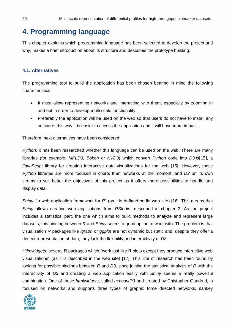
Selections: this is one of the strongest points of D3, that it uses selections. This means that
it costs only one line of code to select one element or a certain group of elements instead of
needing a loop to call them, either to set a property for them or to make them do anything.
That allows really efficient and understandable codes (see Fig 4.1).
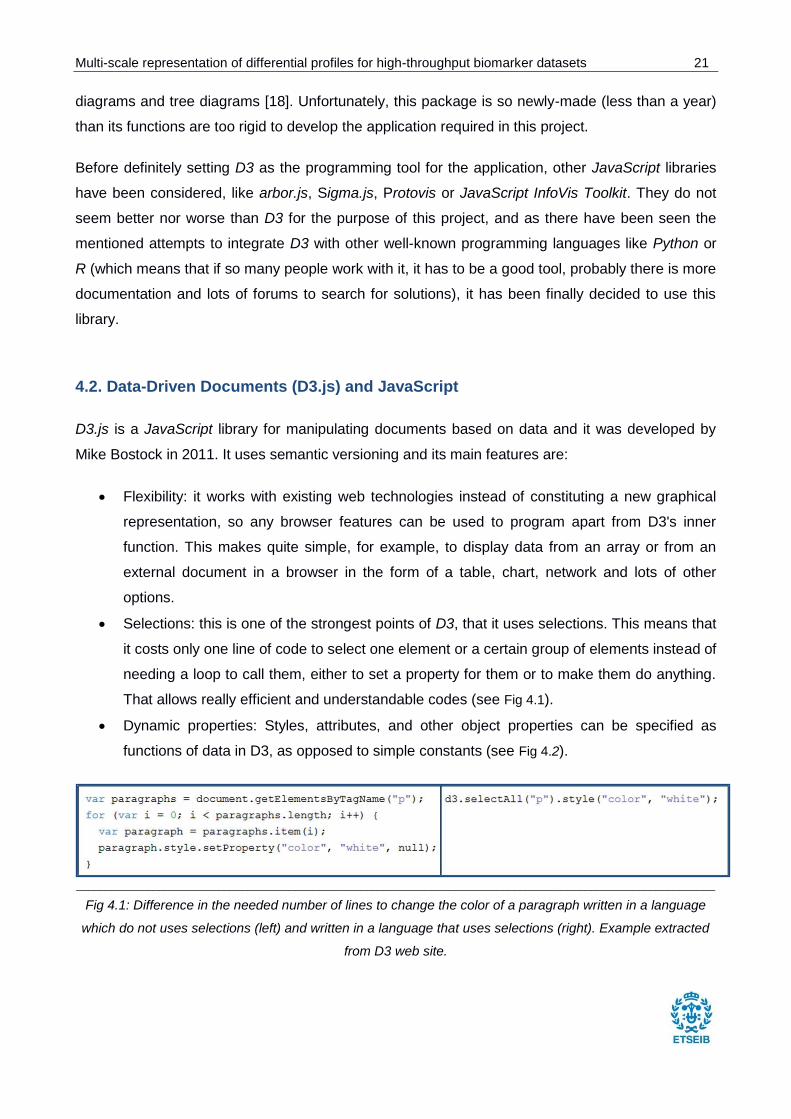
Dynamic properties: Styles, attributes, and other object properties can be specified as
functions of data in D3, as opposed to simple constants (see Fig 4.2).
____________________________________________________________________________________________________________
Fig 4.1: Difference in the needed number of lines to change the color of a paragraph written in a language
which do not uses selections (left) and written in a language that uses selections (right). Example extracted
from D3 web site.
22 Multi-scale representation of differential profiles for high-throughput biomarker datasets
____________________________________________________________________________________________________________
Fig 4.2: two ways of applying color to several elements with D3. Left command will make all paragraphs
show in white color while right command will make them appear in different random colors.
As for its structure, D3 classifies all its functions in the following groups:
Core: fundamental functions for manipulating data. At the same time, this group is divided
in selections, transitions, arrays, math, external resources, string formating, localization and
colors.
Scales: functions that map from an input domain to an output range. They can be
quantitative (for continuous input domains, such as numbers), ordinal (for discrete input
domains, such as names or categories) or time scales (for time domains) and each one has
its own functions.
SVG: utilities for creating Scalable Vector Graphics.
Behaviors: functions containing dragging and zooming properties.
Layouts: algorithms and heuristics to output a set of input data in cohesive
positions/shapes.
Geometry: utilities for 2D geometry.
Geography: project spherical coordinates, latitude and longitude math.
Time: parse or format times, compute calendar intervals, etc.
Regarding JavaScript, it is not the intention of the project to enter into a detailed explanation about
its operation but to stand out two important characteristics:
It does not follow sequential execution of program code, unlike C or C++ or Java. While in
these languages each command starts only after prior has finished, in JavaScript each
command starts after prior has started. This means that if prior command is longer than
current command, some errors can occur if current command depends on results of prior
command. In order to avoid this, it is necessary to apply JavaScript methods to delay the
start of certain commands and build asynchronous code instead of synchronous one, which
can be achieved with callbacks.
To view a web site, code must be written in an .html document. In this .html file, the web
site is edited by tags. For example, inside the <body> tag of the page user can insert
headers, buttons, paragraphs... Inside the <style> tag user can set attributes for certain
Multi-scale representation of differential profiles for high-throughput biomarker datasets 23
elements, etc. Inside a <script> tag there must be a call like this one to D3 library in order to
work with it: <script src="http://d3js.org/d3.v3.min.js"></script>. And if the user wants to call
a function located in an external document (JavaScript documents use .js extension), he or
she must include another <script> tag like this one (assuming external document is called
plot.js): <script src="plot.js"></script>
4.3. Prototype building
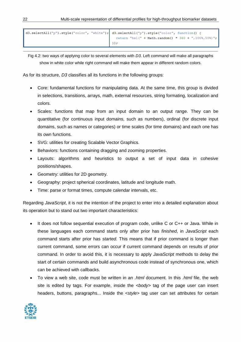
Fig 4.3 shows the prototype which was built as an example for the interviews. It consists in a
simple web page with a 960*500 area of visualization and a small interactive network (eight nodes
and seven links) inside. This interactivity means that the user can drag nodes, zoom in and zoom
out the graph (which apart from increasing and decreasing nodes’ size makes nodes and links
appear and disappear) and view the name of each node by placing the mouse over them.
____________________________________________________________________________________________________________
Fig 4.3: Prototype which was shown to all interviewees. When scale is less than 2 (left picture) only nodes
from group 1 are visible and when scale is greater than 2 (right picture) all of them appear in the browser.
It is important to understand how this zoom process works since it constitutes the base of multi-
scale feature of the application. At every mouse wheel movement the rectangle which contains the
graph is redrawn bigger or smaller and the information to redraw it is obtained by two parameters
[19]:
d3.event.translate: this parameter gives left and top position of the rectangle, bearing in
mind that first time graph is displayed these values are both zero and when scale is
24 Multi-scale representation of differential profiles for high-throughput biomarker datasets
different from 1 new values are expressed in the coordinates of new scale. Manipulating
this translate parameter can be a bit confusing since nodes always maintain the first
coordinate system position while rectangle position is always expressed based on the new
coordinate system. In other words: nodes positions are independent from the coordinate
system and rectangle position depends on it.
d3.event.scale: first time graph is displayed, meaning when the web site is opened,
rectangle is represented at scale 1, so mouse wheel forward movement increases this
scale making the graph bigger and mouse wheel backward movement decreases the scale
making the graph smaller.
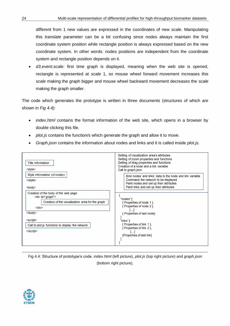
The code which generates the prototype is written in three documents (structures of which are
shown in Fig 4.4):
index.html contains the format information of the web site, which opens in a browser by
double clicking this file.
plot.js contains the function/s which generate the graph and allow it to move.
Graph.json contains the information about nodes and links and it is called inside plot.js.
____________________________________________________________________________________________________________
Fig 4.4: Structure of prototype’s code. index.html (left picture), plot.js (top right picture) and graph.json
(bottom right picture).

Multi-scale representation of differential profiles for high-throughput biomarker datasets 25
5. Specific requirements
This chapter analyses the three interviews which took place in order to get specific requirements
for the application. These requirements are summarized at the end of the chapter and interviews
can be found in Appendix A.
All interviewees were shown the example web site mentioned in section 3.3, they were requested
to interact with it and they were asked the same three questions:
1. Which options and functionalities would you like this application to have?
2. In which format do you have the data to enter to the application?
3. Which program are you using at the moment to display data and why does it not meet your
needs?
5.1. Interview 1
The interviewee is a researcher in bioinformatics and he is working with big networks of
metabolites and graphs with metabolomics data. He mainly works with KEGG database, visualizing
relations between its elements as networks where pathways, modules, enzymes, reactions and
compounds are nodes and connections are links between them.
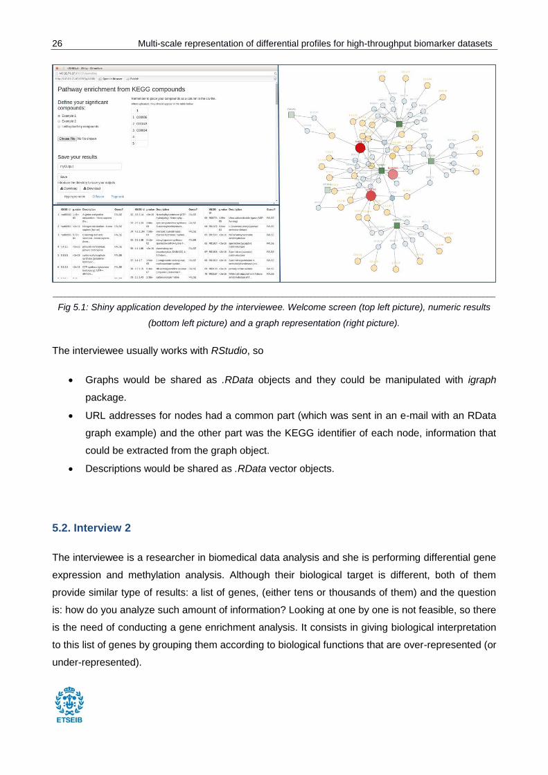
At the moment he is using a Shiny application of his own to represent static networks images and
also make some calculations on them. Reader will find a picture of the Shiny application in Fig 5.1.
The only thing this application lacks is interactivity in the display, that is what he said he needs in
the new application. Therefore, when playing with the example, asked functionalities had to do
essentially with visualization:
To see nodes’ names permanently, not when the mouse goes over them.
To see information about a selected node.
To connect with KEGG’s web site when double clicking a node.
To make nodes appear and disappear.
To save subgraphs.
To be able to make annotations.
To add lost connections.
To search a node.
To change color of nodes.
26 Multi-scale representation of differential profiles for high-throughput biomarker datasets
____________________________________________________________________________________________________________
Fig 5.1: Shiny application developed by the interviewee. Welcome screen (top left picture), numeric results
(bottom left picture) and a graph representation (right picture).
The interviewee usually works with RStudio, so
Graphs would be shared as .RData objects and they could be manipulated with igraph
package.
URL addresses for nodes had a common part (which was sent in an e-mail with an RData
graph example) and the other part was the KEGG identifier of each node, information that
could be extracted from the graph object.
Descriptions would be shared as .RData vector objects.
5.2. Interview 2
The interviewee is a researcher in biomedical data analysis and she is performing differential gene
expression and methylation analysis. Although their biological target is different, both of them
provide similar type of results: a list of genes, (either tens or thousands of them) and the question
is: how do you analyze such amount of information? Looking at one by one is not feasible, so there
is the need of conducting a gene enrichment analysis. It consists in giving biological interpretation
to this list of genes by grouping them according to biological functions that are over-represented (or
under-represented).
Multi-scale representation of differential profiles for high-throughput biomarker datasets 27
The interviewee mainly works with three databases: KEGG PATHWAY, Reactome and The Gene
Ontology (GO).
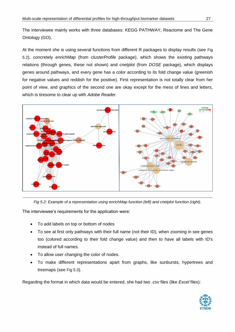
At the moment she is using several functions from different R packages to display results (see Fig
5.2), concretely enrichMap (from clusterProfile package), which shows the existing pathways
relations (through genes, these not shown) and cnetplot (from DOSE package), which displays
genes around pathways, and every gene has a color according to its fold change value (greenish
for negative values and reddish for the positive). First representation is not totally clear from her
point of view, and graphics of the second one are okay except for the mess of lines and letters,
which is tiresome to clear up with Adobe Reader.
____________________________________________________________________________________________________________
Fig 5.2: Example of a representation using enrichMap function (left) and cnetplot function (right).
The interviewee’s requirements for the application were:
To add labels on top or bottom of nodes
To see at first only pathways with their full name (not their ID), when zooming in see genes
too (colored according to their fold change value) and then to have all labels with ID's
instead of full names.
To allow user changing the color of nodes.
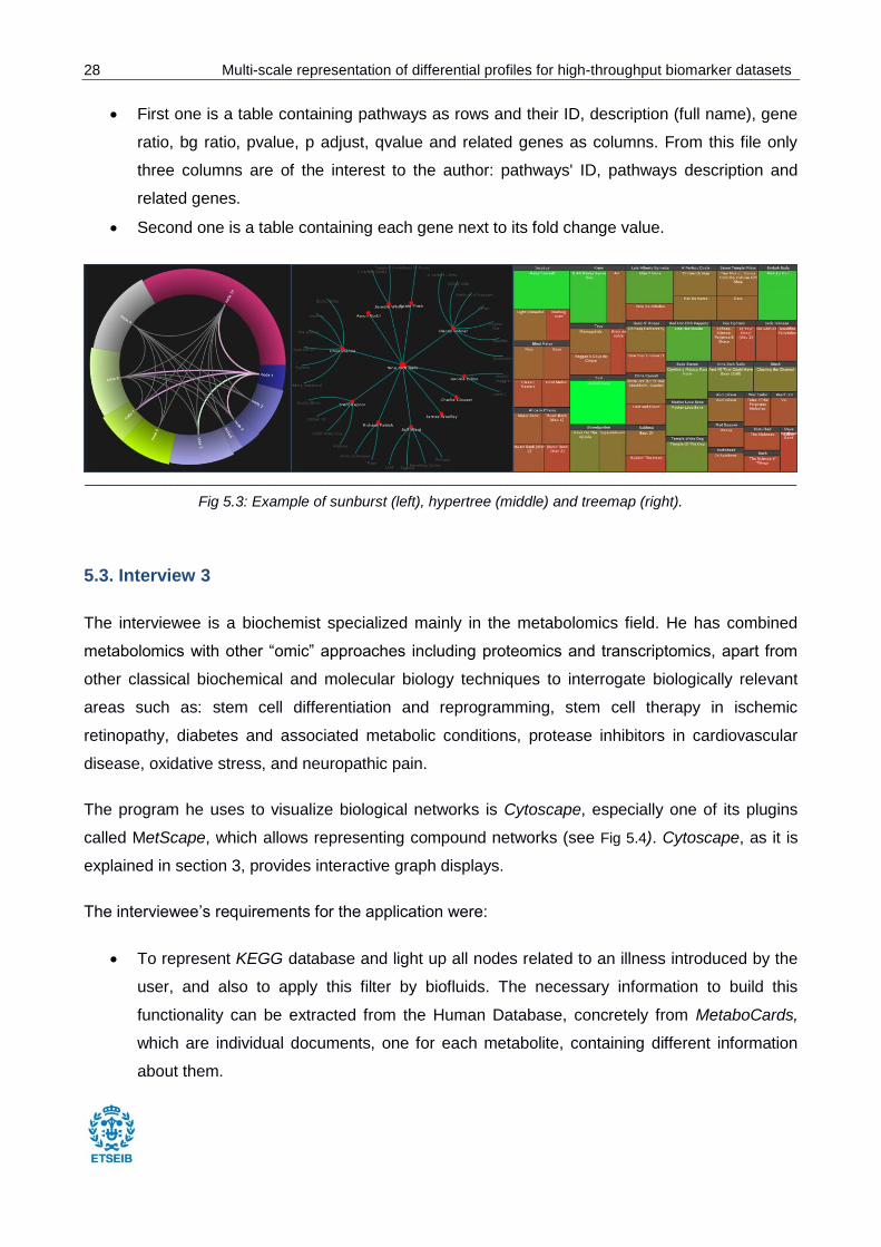
To make different representations apart from graphs, like sunbursts, hypertrees and
treemaps (see Fig 5.3).
Regarding the format in which data would be entered, she had two .csv files (like Excel files):
28 Multi-scale representation of differential profiles for high-throughput biomarker datasets
First one is a table containing pathways as rows and their ID, description (full name), gene
ratio, bg ratio, pvalue, p adjust, qvalue and related genes as columns. From this file only
three columns are of the interest to the author: pathways' ID, pathways description and
related genes.
Second one is a table containing each gene next to its fold change value.
____________________________________________________________________________________________________________
Fig 5.3: Example of sunburst (left), hypertree (middle) and treemap (right).
5.3. Interview 3
The interviewee is a biochemist specialized mainly in the metabolomics field. He has combined
metabolomics with other “omic” approaches including proteomics and transcriptomics, apart from
other classical biochemical and molecular biology techniques to interrogate biologically relevant
areas such as: stem cell differentiation and reprogramming, stem cell therapy in ischemic
retinopathy, diabetes and associated metabolic conditions, protease inhibitors in cardiovascular
disease, oxidative stress, and neuropathic pain.
The program he uses to visualize biological networks is Cytoscape, especially one of its plugins
called MetScape, which allows representing compound networks (see Fig 5.4). Cytoscape, as it is
explained in section 3, provides interactive graph displays.
The interviewee’s requirements for the application were:
To represent KEGG database and light up all nodes related to an illness introduced by the
user, and also to apply this filter by biofluids. The necessary information to build this
functionality can be extracted from the Human Database, concretely from MetaboCards,
which are individual documents, one for each metabolite, containing different information
about them.
Multi-scale representation of differential profiles for high-throughput biomarker datasets 29
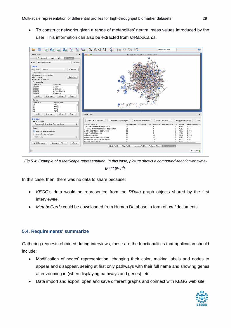
To construct networks given a range of metabolites’ neutral mass values introduced by the
user. This information can also be extracted from MetaboCards.
____________________________________________________________________________________________________________
Fig 5.4: Example of a MetScape representation. In this case, picture shows a compound-reaction-enzyme-
gene graph.
In this case, then, there was no data to share because:
KEGG’s data would be represented from the RData graph objects shared by the first
interviewee.
MetaboCards could be downloaded from Human Database in form of .xml documents.
5.4. Requirements' summarize
Gathering requests obtained during interviews, these are the functionalities that application should
include:
Modification of nodes’ representation: changing their color, making labels and nodes to
appear and disappear, seeing at first only pathways with their full name and showing genes
after zooming in (when displaying pathways and genes), etc.
Data import and export: open and save different graphs and connect with KEGG web site.

30 Multi-scale representation of differential profiles for high-throughput biomarker datasets
Information filters: allow the user to create or stand out subgraphs by selecting metabolites
according to a specific range of mass values, diseases and/or biofluids.
Manual annotations: allowing the user to make annotations about a node or the network in
general and search a concrete node.
Without forgetting these previous requirements:
Implement a multi-scale feature.
Embed the program on an R package in which B2SLab is working at the moment.
Multi-scale representation of differential profiles for high-throughput biomarker datasets 31
6. Design and development of the application
The application is clearly divided in two parts: the one that displays and manipulates graphs with
few nodes and the one that displays and manipulates graphs with lots of nodes. This one word that
changes from one part to another means a great difference at the time of designing the application,
since when working with few nodes they can be represented all at once with D3, while rendering
lots of them would crash the computer and, therefore, alternative methods must be built to face the
problem. Here is where the multi-scale visualization feature of the application gains relevance and
chapter 7 describes in detail how it has been implemented. This feature is also what gives the
program its name: BiMS Viewer, which means Biomedical Multi-Scale Viewer. That said, this
chapter explains the general appearance and operating of BiMS considering networks with less
than 500 nodes (approaching this limit may make the application run slowly) and also deals with
data entering format.
6.1. Appearance and operation
The structure of the application consists in a row of buttons at the top of the browser (these are the
visualization controllers) and another one at the bottom (the extended controllers), the rest of the
screen assigned to the networks' representation area. Since the application is a visualizer, this
distribution of space intends to give the greatest room possible to graphs display in order to make
easier user's analysis.
6.1.1. Visualization controllers
Visualization controllers are the buttons in charge of opening new networks, so they are always
visible and enabled for whenever the user wishes to study a new graph. These buttons are located
at the top of the screen and they are (from left to right):
Browse: allows the user to open a .json file containing nodes and links information to
construct a network (see section 6.2 for more details about .json format). The file selected
by the user must be located in the same folder as the index.html document because
otherwise the graph cannot be displayed. This is because for security reasons browsers do
not allow to keep the path to a file.
Create Network: allows the user to write a minimum and a maximum mass value (or a
single value) and produces a network with all the compounds of the Human Database the
32 Multi-scale representation of differential profiles for high-throughput biomarker datasets
mass of which is between those values (as long as they have a KEGG identifier). If the
number of nodes to draw is greater than 500, the user is requested to make the range of
mass values smaller so that the application does not freeze.
KEGG's Compounds: creates a graph with the compounds of KEGG's database. As there
are more than 7000 and the browser would crash when trying to render all of them,
compounds have been classified in clusters so that no more than 500 are displayed at the
same time. Chapter 7 explains in detail the procedure which has been used to achieve this.
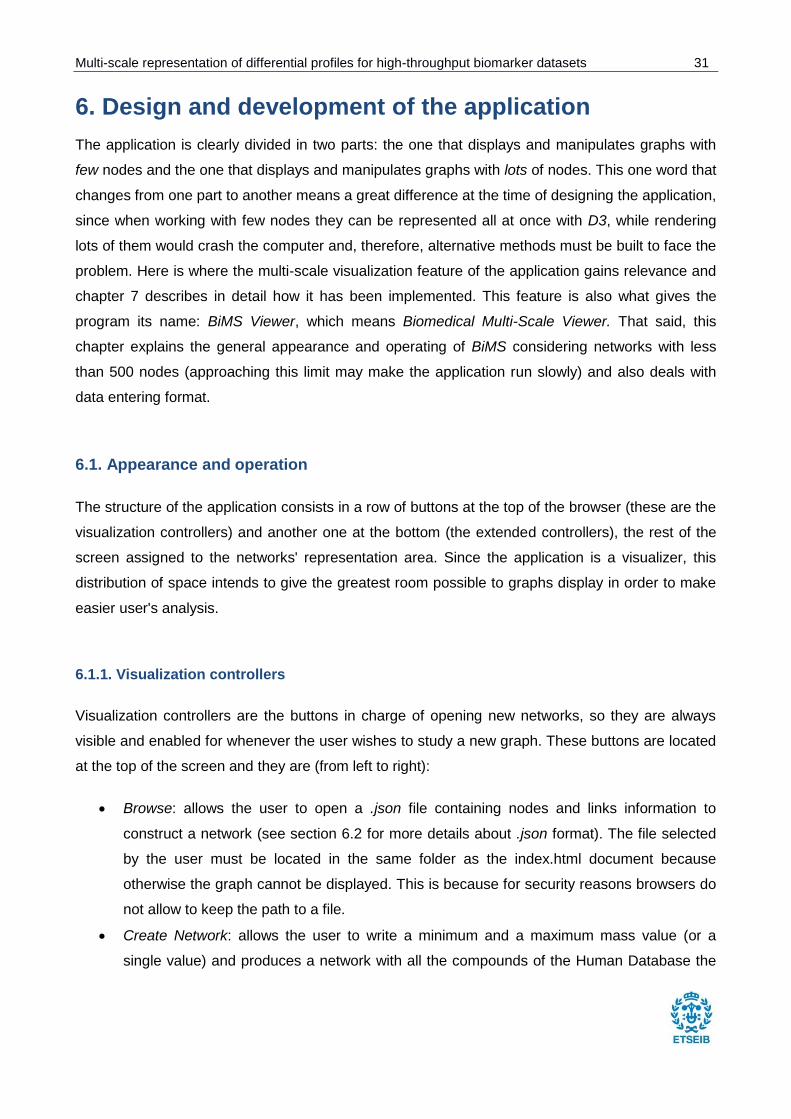
Buttons located at the bottom of the screen (the extended controllers) are in charge of allowing the
interaction with the current graph display, that is why when user opens the application and
welcome screen is shown, only top buttons are visible (see Fig 6.1).
____________________________________________________________________________________________________________
Fig 6.1: Welcome screen of BiMS.
What happens (after clicking Browse button) in the few seconds from when a file is selected to
when the network and the bottom buttons appear? First of all, BiMS verifies if file's format is .json.
When not correct, an alert message is shown and the user returns to the welcome screen. When
correct, the application removes all elements from the visualization area and counts how many
nodes the .json file has:
If it exceeds 500 nodes and they are grouped in clusters, it calls to viewClusters function
(see chapter 7).
If it exceeds 500 nodes but they are not grouped in clusters, an alert message is shown
and the user returns to the welcome screen.
Multi-scale representation of differential profiles for high-throughput biomarker datasets 33
If it does not exceed 500 nodes, it calls to viewNetwork function, which displays the graph.
Create Network’s sequence is shorter than Browse one. It asks the user to insert a range of mass
values in order to select nodes to represent. If these values are between the minimum and
maximum allowed and they mean not to render more than 500 nodes, BiMS removes current
representation and calls to viewNetwork function. Otherwise, an alert message pops up and user
returns to welcome screen.
Finally, Kegg’s Compounds button is the one with the easiest operation, since it always uses the
same data and it does not generate alert messages because the user does not have to input
anything. It only removes current representation, calls viewClusters function and displays Kegg’s
Compounds graph.
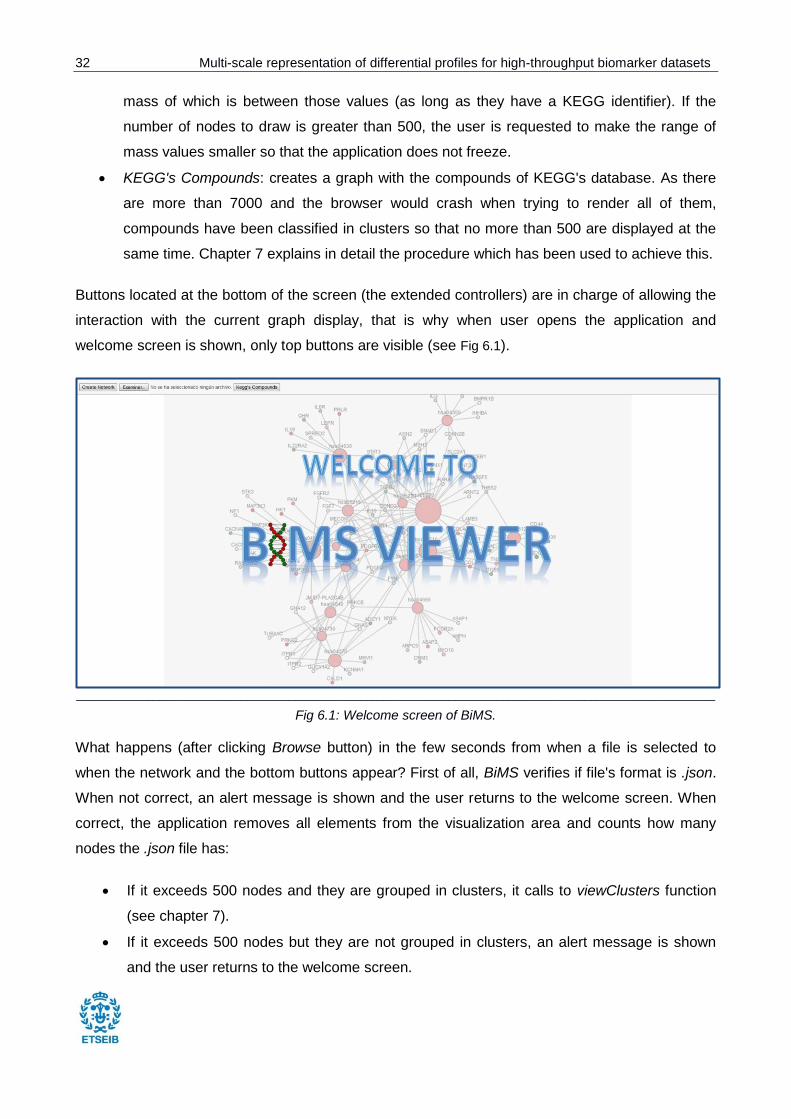
Diagram in Fig 6.2clarifies the above explanation.
____________________________________________________________________________________________________________
Fig 6.2: Diagram showing the operation of the welcome screen’s buttons. Going from left to right, user starts
at welcome screen and depending on his/her actions, BiMS will finish displaying correctly the requested
graph (green rectangles) or it will pop up an alert message explaining why it cannot represent the network
and will return the user to the welcome screen (orange rectangles). Intermediate orders are shown in blue
rectangles.
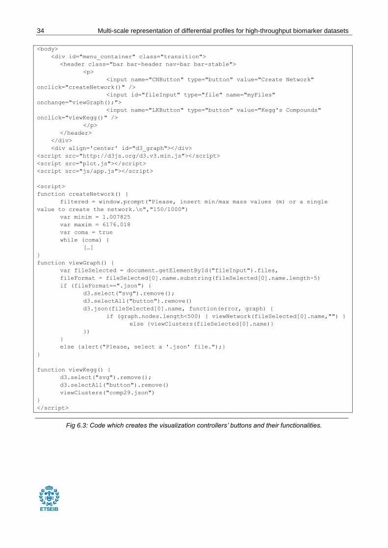
Visualization controllers’ code is located in index.html file because they do not depend on the
graph which is represented, that is why they are edited as web page elements. Fig 6.3 shows part
of the code which creates and builds their functionalities (full code is shown in Appendix B).
34 Multi-scale representation of differential profiles for high-throughput biomarker datasets
<body>
<div id="menu_container" class="transition">
<header class="bar bar-header nav-bar bar-stable">
<p>
<input name="CNButton" type="button" value="Create Network"
onclick="createNetwork()" />
<input id="fileInput" type="file" name="myFiles"
onchange="viewGraph();">
<input name="LKButton" type="button" value="Kegg's Compounds"
onclick="viewKegg()" />
</p>
</header>
</div>
<div align='center' id="d3_graph"></div>
<script src="http://d3js.org/d3.v3.min.js"></script>
<script src="plot.js"></script>
<script src="js/app.js"></script>
<script>
function createNetwork() {
filtered = window.prompt("Please, insert min/max mass values (m) or a single
value to create the network.\n","150/1000")
var minim = 1.007825
var maxim = 6176.018
var coma = true
while (coma) {
[…]
}
function viewGraph() {
var fileSelected = document.getElementById("fileInput").files,
fileFormat = fileSelected[0].name.substring(fileSelected[0].name.length-5)
if (fileFormat==".json") {
d3.select("svg").remove();
d3.selectAll("button").remove()
d3.json(fileSelected[0].name, function(error, graph) {
if (graph.nodes.length<500) { viewNetwork(fileSelected[0].name,"") }
else {viewClusters(fileSelected[0].name)}
})
}
else {alert("Please, select a '.json' file.");}
}
function viewKegg() {
d3.select("svg").remove();
d3.selectAll("button").remove()
viewClusters("comp29.json")
}
</script>
____________________________________________________________________________________________________________
Fig 6.3: Code which creates the visualization controllers’ buttons and their functionalities.
Multi-scale representation of differential profiles for high-throughput biomarker datasets 35
As reader can see, button rectangles are created between tags, concretely inside a paragraph
(<p>) which is inside the <header>, which is at the same time inside the <body> of the web page.
The “value” parameter of each line is the name that appears on each button (meaning the name
that the user sees, like Create Network) and the “on change” parameter calls to the corresponding
function which gives use to the button. Functions are located inside the <script> tag and they
contain the code responsible of the orders shown in Fig 6.2.
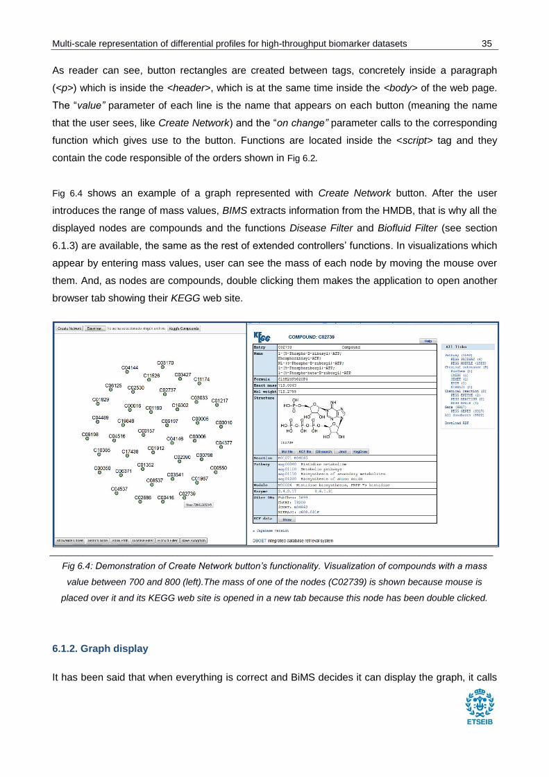
Fig 6.4 shows an example of a graph represented with Create Network button. After the user
introduces the range of mass values, BIMS extracts information from the HMDB, that is why all the
displayed nodes are compounds and the functions Disease Filter and Biofluid Filter (see section
6.1.3) are available, the same as the rest of extended controllers’ functions. In visualizations which
appear by entering mass values, user can see the mass of each node by moving the mouse over
them. And, as nodes are compounds, double clicking them makes the application to open another
browser tab showing their KEGG web site.
____________________________________________________________________________________________________________
Fig 6.4: Demonstration of Create Network button’s functionality. Visualization of compounds with a mass
value between 700 and 800 (left).The mass of one of the nodes (C02739) is shown because mouse is
placed over it and its KEGG web site is opened in a new tab because this node has been double clicked.
6.1.2. Graph display
It has been said that when everything is correct and BiMS decides it can display the graph, it calls
36 Multi-scale representation of differential profiles for high-throughput biomarker datasets
to viewNetwork or viewClusters (both located in plot.js file) after removing the current
representation. It is worth looking at how viewNetwork works (see section 7.4 for viewClusters
code description) before dealing with extended controllers, since it is the responsible function of
making the networks appear.
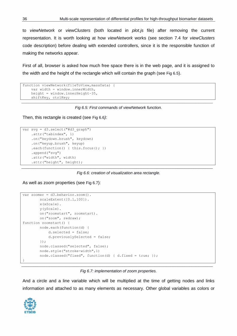
First of all, browser is asked how much free space there is in the web page, and it is assigned to
the width and the height of the rectangle which will contain the graph (see Fig 6.5).
function viewNetwork(fileToView,massData) {
var width = window.innerWidth,
height = window.innerHeight-35,
shiftKey, ctrlKey;
____________________________________________________________________________________________________________
Fig 6.5: First commands of viewNetwork function.
Then, this rectangle is created (see Fig 6.6):
var svg = d3.select("#d3_graph")
.attr("tabindex", 1)
.on("keydown.brush", keydown)
.on("keyup.brush", keyup)
.each(function() { this.focus(); })
.append("svg")
.attr("width", width)
.attr("height", height);
____________________________________________________________________________________________________________
Fig 6.6: creation of visualization area rectangle.
As well as zoom properties (see Fig 6.7):
var zoomer = d3.behavior.zoom().
scaleExtent([0.1,100]).
x(xScale).
y(yScale).
on("zoomstart", zoomstart).
on("zoom", redraw);
function zoomstart() {
node.each(function(d) {
d.selected = false;
d.previouslySelected = false;
});
node.classed("selected", false);
node.style("stroke-width",1)
node.classed("fixed", function(d) { d.fixed = true; });
}
____________________________________________________________________________________________________________
Fig 6.7: implementation of zoom properties.
And a circle and a line variable which will be multiplied at the time of getting nodes and links
information and attached to as many elements as necessary. Other global variables as colors or
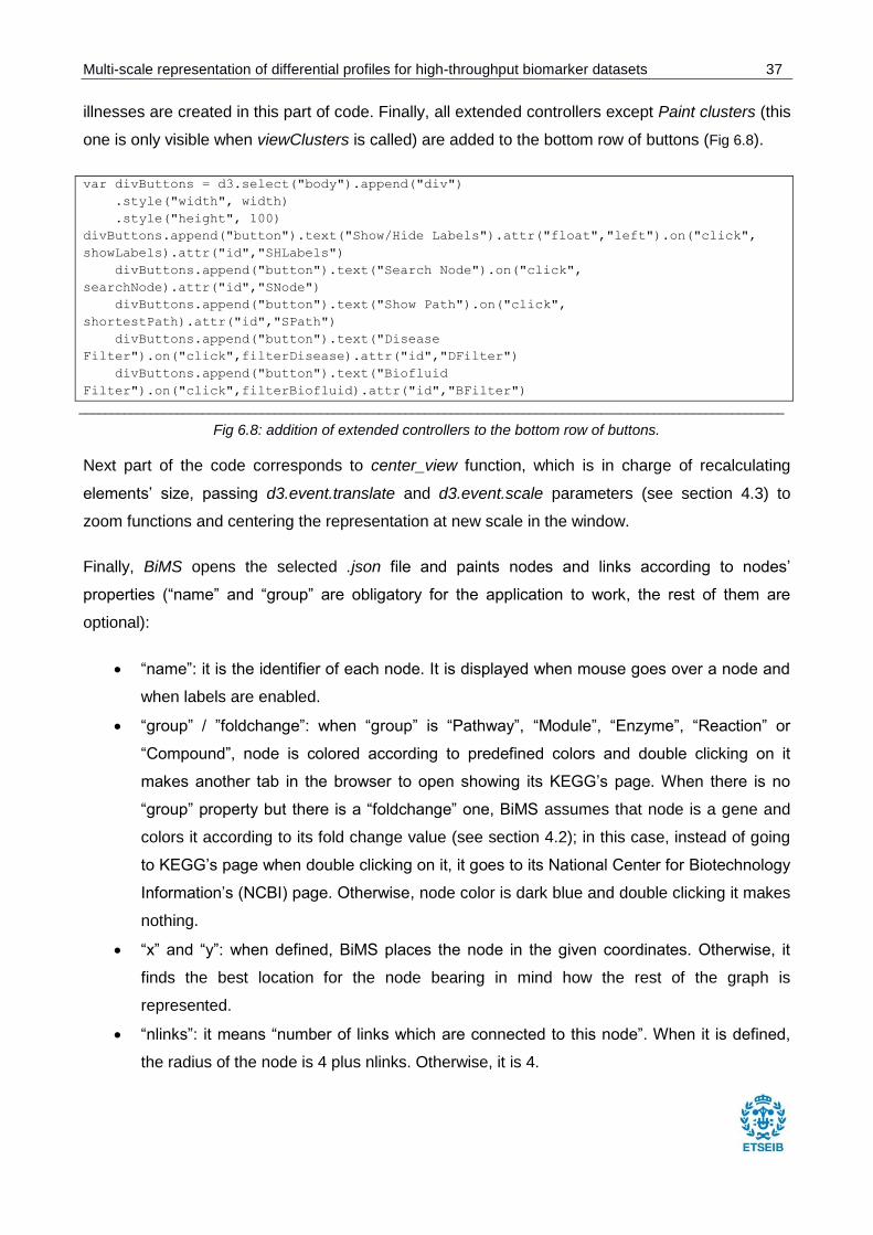
Multi-scale representation of differential profiles for high-throughput biomarker datasets 37
illnesses are created in this part of code. Finally, all extended controllers except Paint clusters (this
one is only visible when viewClusters is called) are added to the bottom row of buttons (Fig 6.8).
var divButtons = d3.select("body").append("div")
.style("width", width)
.style("height", 100)
divButtons.append("button").text("Show/Hide Labels").attr("float","left").on("click",
showLabels).attr("id","SHLabels")
divButtons.append("button").text("Search Node").on("click",
searchNode).attr("id","SNode")
divButtons.append("button").text("Show Path").on("click",
shortestPath).attr("id","SPath")
divButtons.append("button").text("Disease
Filter").on("click",filterDisease).attr("id","DFilter")
divButtons.append("button").text("Biofluid
Filter").on("click",filterBiofluid).attr("id","BFilter")
____________________________________________________________________________________________________________
Fig 6.8: addition of extended controllers to the bottom row of buttons.
Next part of the code corresponds to center_view function, which is in charge of recalculating
elements’ size, passing d3.event.translate and d3.event.scale parameters (see section 4.3) to
zoom functions and centering the representation at new scale in the window.
Finally, BiMS opens the selected .json file and paints nodes and links according to nodes’
properties (“name” and “group” are obligatory for the application to work, the rest of them are
optional):
“name”: it is the identifier of each node. It is displayed when mouse goes over a node and
when labels are enabled.
“group” / ”foldchange”: when “group” is “Pathway”, “Module”, “Enzyme”, “Reaction” or
“Compound”, node is colored according to predefined colors and double clicking on it
makes another tab in the browser to open showing its KEGG’s page. When there is no
“group” property but there is a “foldchange” one, BiMS assumes that node is a gene and
colors it according to its fold change value (see section 4.2); in this case, instead of going
to KEGG’s page when double clicking on it, it goes to its National Center for Biotechnology
Information’s (NCBI) page. Otherwise, node color is dark blue and double clicking it makes
nothing.
“x” and “y”: when defined, BiMS places the node in the given coordinates. Otherwise, it
finds the best location for the node bearing in mind how the rest of the graph is
represented.
“nlinks”: it means “number of links which are connected to this node”. When it is defined,
the radius of the node is 4 plus nlinks. Otherwise, it is 4.
38 Multi-scale representation of differential profiles for high-throughput biomarker datasets
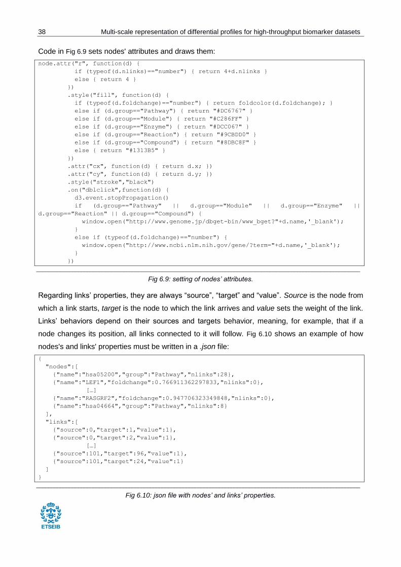
Code in Fig 6.9 sets nodes' attributes and draws them:
node.attr("r", function(d) {
if (typeof(d.nlinks)=="number") { return 4+d.nlinks }
else { return 4 }
})
.style("fill", function(d) {
if (typeof(d.foldchange)=="number") { return foldcolor(d.foldchange); }
else if (d.group=="Pathway") { return "#DC6767" }
else if (d.group=="Module") { return "#C286FF" }
else if (d.group=="Enzyme") { return "#DCC067" }
else if (d.group=="Reaction") { return "#9CBDD0" }
else if (d.group=="Compound") { return "#8DBC8F" }
else { return "#1313B5" }
})
.attr("cx", function(d) { return d.x; })
.attr("cy", function(d) { return d.y; })
.style("stroke","black")
.on("dblclick",function(d) {
d3.event.stopPropagation()
if (d.group=="Pathway" || d.group=="Module" || d.group=="Enzyme" ||
d.group=="Reaction" || d.group=="Compound") {
window.open("http://www.genome.jp/dbget-bin/www_bget?"+d.name,'_blank');
}
else if (typeof(d.foldchange)=="number") {
window.open("http://www.ncbi.nlm.nih.gov/gene/?term="+d.name,'_blank');
}
})
____________________________________________________________________________________________________________
Fig 6.9: setting of nodes’ attributes.
Regarding links’ properties, they are always “source”, “target” and “value”. Source is the node from
which a link starts, target is the node to which the link arrives and value sets the weight of the link.
Links’ behaviors depend on their sources and targets behavior, meaning, for example, that if a
node changes its position, all links connected to it will follow. Fig 6.10 shows an example of how
nodes's and links' properties must be written in a .json file:
{
"nodes":[
{"name":"hsa05200","group":"Pathway","nlinks":28},
{"name":"LEF1","foldchange":0.766911362297833,"nlinks":0},
[…]
{"name":"RASGRF2","foldchange":0.947706323349848,"nlinks":0},
{"name":"hsa04664","group":"Pathway","nlinks":8}
],
"links":[
{"source":0,"target":1,"value":1},
{"source":0,"target":2,"value":1},
[…]
{"source":101,"target":96,"value":1},
{"source":101,"target":24,"value":1}
]
}
____________________________________________________________________________________________________________
Fig 6.10: json file with nodes’ and links’ properties.
Multi-scale representation of differential profiles for high-throughput biomarker datasets 39
6.1.3. Extended controllers
Once the application has been opened, a file has been selected and a network has been
represented, extended buttons come into play. They all apply changes to the graph and have been
created according to specific requirements extracted from interviews (see section 5.4). All of them
are always visible but not enabled, because that depends on the characteristics of each network.
The ones always enabled are:
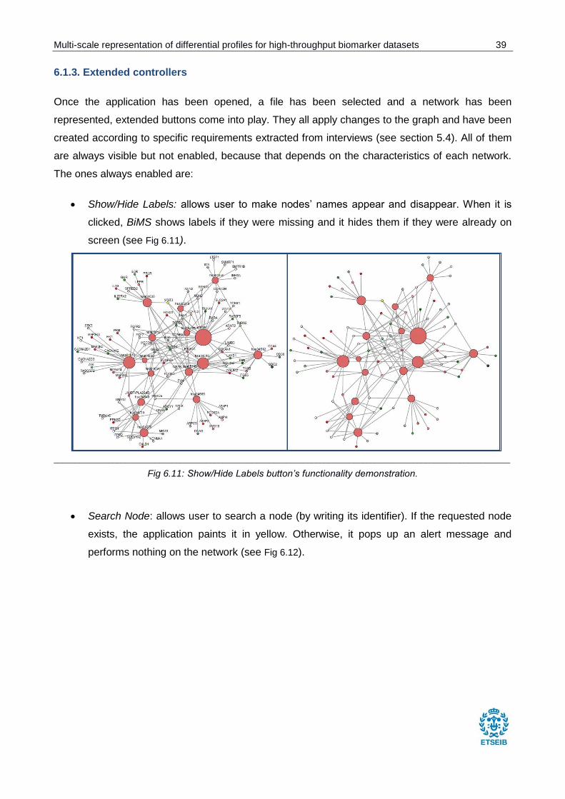
Show/Hide Labels: allows user to make nodes’ names appear and disappear. When it is
clicked, BiMS shows labels if they were missing and it hides them if they were already on
screen (see Fig 6.11).
____________________________________________________________________________________________________________
Fig 6.11: Show/Hide Labels button’s functionality demonstration.
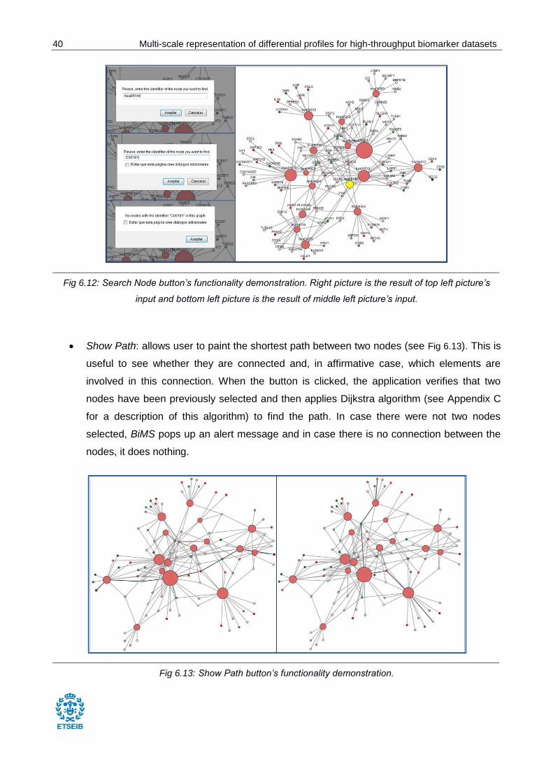
Search Node: allows user to search a node (by writing its identifier). If the requested node
exists, the application paints it in yellow. Otherwise, it pops up an alert message and
performs nothing on the network (see Fig 6.12).
40 Multi-scale representation of differential profiles for high-throughput biomarker datasets
____________________________________________________________________________________________________________
Fig 6.12: Search Node button’s functionality demonstration. Right picture is the result of top left picture’s
input and bottom left picture is the result of middle left picture’s input.
Show Path: allows user to paint the shortest path between two nodes (see Fig 6.13). This is
useful to see whether they are connected and, in affirmative case, which elements are
involved in this connection. When the button is clicked, the application verifies that two
nodes have been previously selected and then applies Dijkstra algorithm (see Appendix C
for a description of this algorithm) to find the path. In case there were not two nodes
selected, BiMS pops up an alert message and in case there is no connection between the
nodes, it does nothing.
____________________________________________________________________________________________________________
Fig 6.13: Show Path button’s functionality demonstration.
Multi-scale representation of differential profiles for high-throughput biomarker datasets 41
Disease Filter and Biofluid Filter are only enabled when the displayed network has compounds as
nodes. This is because they need to search information in the HMDB MetaboCards to work, and
MetaboCards contain only compounds’ properties. That said, these two buttons’ functionalities are
very similar:
Disease Filter allows finding which compounds are related to an illness. There is also the
possibility to find which compounds are in a specific biofluid when they are related to an
illness. This depends on the format in which the user introduces the search, which can be
either disease/biofluid or simply disease. Disease Filter has been implemented in a quite
flexible way in order to make user’s experience as comfortable as possible, meaning that:
o No matter if input is made in capital letters or lower case letters.
o No matter if user does not write an entire word provided that there is only one
disease containing the letters he/she has introduced. For example: BiMS will accept
either Alzheimer or Alz as an input and will show the same results because there is
only one disease (Alzheimer’s Disease according to HMDB) which contains Alz
combination.
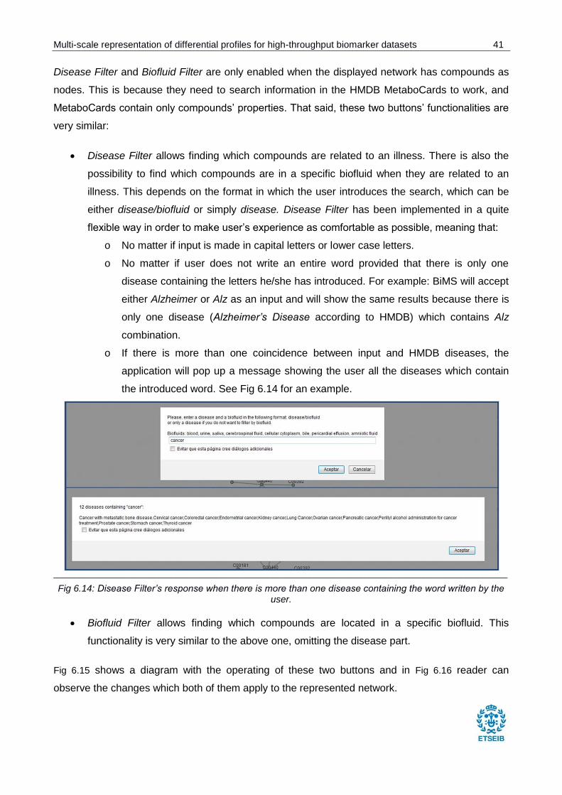
o If there is more than one coincidence between input and HMDB diseases, the
application will pop up a message showing the user all the diseases which contain
the introduced word. See Fig 6.14 for an example.
____________________________________________________________________________________________________________
Fig 6.14: Disease Filter’s response when there is more than one disease containing the word written by the user.
Biofluid Filter allows finding which compounds are located in a specific biofluid. This
functionality is very similar to the above one, omitting the disease part.
Fig 6.15 shows a diagram with the operating of these two buttons and in Fig 6.16 reader can
observe the changes which both of them apply to the represented network.
42 Multi-scale representation of differential profiles for high-throughput biomarker datasets
____________________________________________________________________________________________________________
Fig 6.15: Diagram showing the operation of Disease Filter button and Biofluid Filter button. Going from left to
right, user starts with a graph displayed and depending on his/her actions, BiMS will finish recoloring nodes
according to the disease/biofluid (or both) requested (green rectangles) or it will pop up an alert message
explaining why it cannot apply changes to the network and will return the user to the graph display screen
without modifications (orange rectangles). Intermediate orders are shown in blue rectangles.
____________________________________________________________________________________________________________
Fig 6.16: Disease Filter button’s functionality demonstration. Left picture shows which compounds are
related to AIDS in the displayed network, middle picture shows which ones are related to AIDS in blood and
right picture shows which ones are related to AIDS in cerebrospinal fluid.
Remainder button, which is Save Subgraph, creates a json file with the properties of the
represented graph so that the user can download it. It would not make sense to open a file and
save it again in another file, that is why this button is only enabled in the following situations:
The graph has been generated with the Create Network button. As the user does not have
a file with this network because it has been created from mass values, the application offers
to save it for future times.
Biofluid Filter or Disease Filter have been applied. In both cases, BiMS saves in a new file
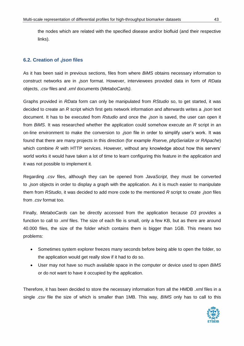
Multi-scale representation of differential profiles for high-throughput biomarker datasets 43
the nodes which are related with the specified disease and/or biofluid (and their respective
links).
6.2. Creation of .json files
As it has been said in previous sections, files from where BiMS obtains necessary information to
construct networks are in .json format. However, interviewees provided data in form of RData
objects, .csv files and .xml documents (MetaboCards).
Graphs provided in RData form can only be manipulated from RStudio so, to get started, it was
decided to create an R script which first gets network information and afterwards writes a .json text
document. It has to be executed from Rstudio and once the .json is saved, the user can open it
from BiMS. It was researched whether the application could somehow execute an R script in an
on-line environment to make the conversion to .json file in order to simplify user’s work. It was
found that there are many projects in this direction (for example Rserve, phpSerialize or RApache)
which combine R with HTTP services. However, without any knowledge about how this servers’
world works it would have taken a lot of time to learn configuring this feature in the application and
it was not possible to implement it.
Regarding .csv files, although they can be opened from JavaScript, they must be converted
to .json objects in order to display a graph with the application. As it is much easier to manipulate
them from RStudio, it was decided to add more code to the mentioned R script to create .json files
from .csv format too.
Finally, MetaboCards can be directly accessed from the application because D3 provides a
function to call to .xml files. The size of each file is small, only a few KB, but as there are around
40.000 files, the size of the folder which contains them is bigger than 1GB. This means two
problems:
Sometimes system explorer freezes many seconds before being able to open the folder, so
the application would get really slow if it had to do so.
User may not have so much available space in the computer or device used to open BiMS
or do not want to have it occupied by the application.
Therefore, it has been decided to store the necessary information from all the HMDB .xml files in a
single .csv file the size of which is smaller than 1MB. This way, BIMS only has to call to this

44 Multi-scale representation of differential profiles for high-throughput biomarker datasets
document and the issues explained above are solved simultaneously.
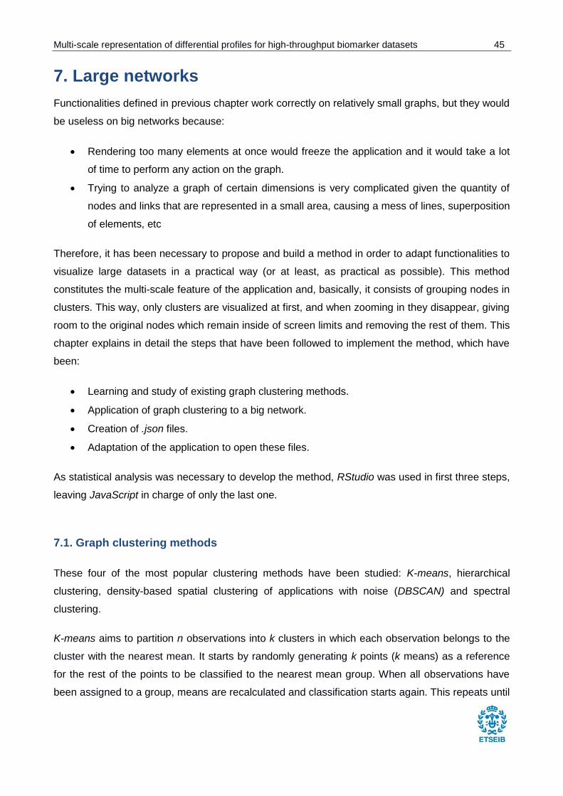
Multi-scale representation of differential profiles for high-throughput biomarker datasets 45
7. Large networks
Functionalities defined in previous chapter work correctly on relatively small graphs, but they would
be useless on big networks because:
Rendering too many elements at once would freeze the application and it would take a lot
of time to perform any action on the graph.
Trying to analyze a graph of certain dimensions is very complicated given the quantity of
nodes and links that are represented in a small area, causing a mess of lines, superposition
of elements, etc
Therefore, it has been necessary to propose and build a method in order to adapt functionalities to
visualize large datasets in a practical way (or at least, as practical as possible). This method
constitutes the multi-scale feature of the application and, basically, it consists of grouping nodes in
clusters. This way, only clusters are visualized at first, and when zooming in they disappear, giving
room to the original nodes which remain inside of screen limits and removing the rest of them. This
chapter explains in detail the steps that have been followed to implement the method, which have
been:
Learning and study of existing graph clustering methods.
Application of graph clustering to a big network.
Creation of .json files.
Adaptation of the application to open these files.
As statistical analysis was necessary to develop the method, RStudio was used in first three steps,
leaving JavaScript in charge of only the last one.
7.1. Graph clustering methods
These four of the most popular clustering methods have been studied: K-means, hierarchical
clustering, density-based spatial clustering of applications with noise (DBSCAN) and spectral
clustering.
K-means aims to partition n observations into k clusters in which each observation belongs to the
cluster with the nearest mean. It starts by randomly generating k points (k means) as a reference
for the rest of the points to be classified to the nearest mean group. When all observations have
been assigned to a group, means are recalculated and classification starts again. This repeats until
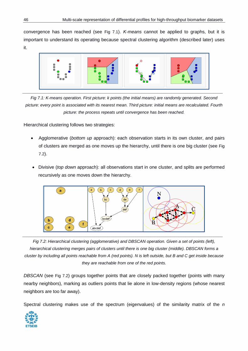
46 Multi-scale representation of differential profiles for high-throughput biomarker datasets
convergence has been reached (see Fig 7.1). K-means cannot be applied to graphs, but it is
important to understand its operating because spectral clustering algorithm (described later) uses
it.
____________________________________________________________________________________________________________
Fig 7.1: K-means operation. First picture: k points (the initial means) are randomly generated. Second
picture: every point is associated with its nearest mean. Third picture: initial means are recalculated. Fourth
picture: the process repeats until convergence has been reached.
Hierarchical clustering follows two strategies:
Agglomerative (bottom up approach): each observation starts in its own cluster, and pairs
of clusters are merged as one moves up the hierarchy, until there is one big cluster (see Fig
7.2).
Divisive (top down approach): all observations start in one cluster, and splits are performed
recursively as one moves down the hierarchy.
____________________________________________________________________________________________________________
Fig 7.2: Hierarchical clustering (agglomerative) and DBSCAN operation. Given a set of points (left),
hierarchical clustering merges pairs of clusters until there is one big cluster (middle). DBSCAN forms a
cluster by including all points reachable from A (red points). N is left outside, but B and C get inside because
they are reachable from one of the red points.
DBSCAN (see Fig 7.2) groups together points that are closely packed together (points with many
nearby neighbors), marking as outliers points that lie alone in low-density regions (whose nearest
neighbors are too far away).
Spectral clustering makes use of the spectrum (eigenvalues) of the similarity matrix of the n
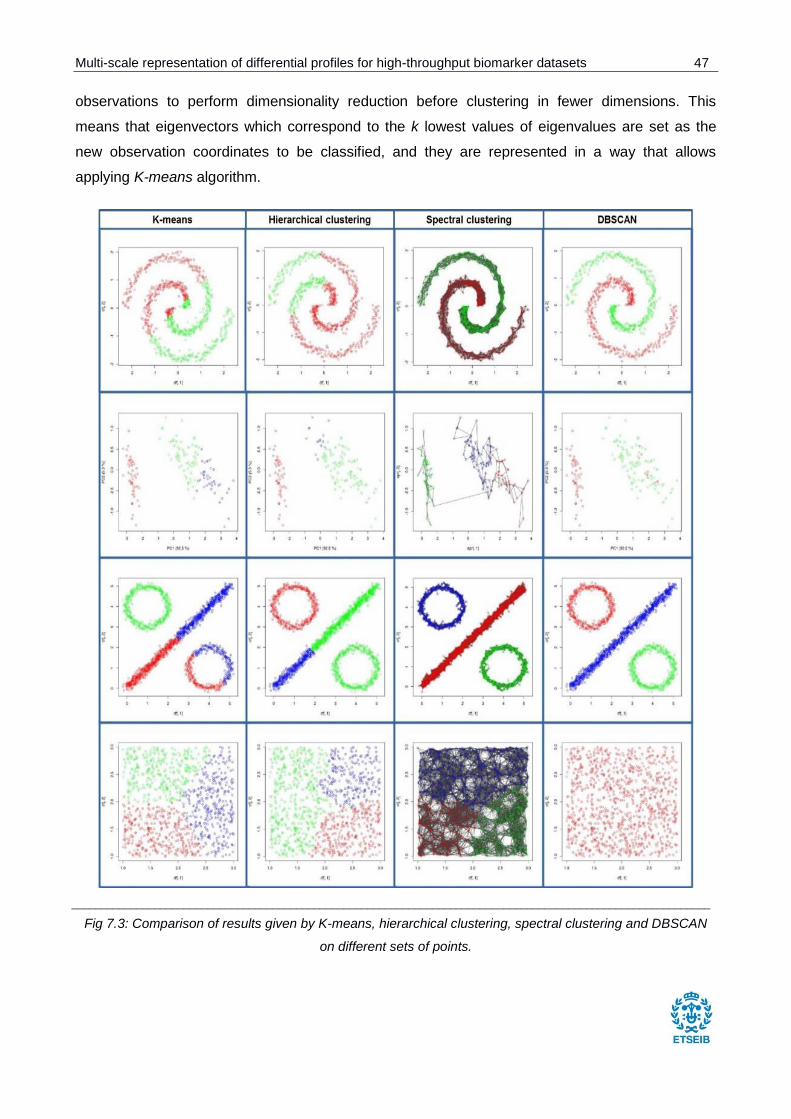
Multi-scale representation of differential profiles for high-throughput biomarker datasets 47
observations to perform dimensionality reduction before clustering in fewer dimensions. This
means that eigenvectors which correspond to the k lowest values of eigenvalues are set as the
new observation coordinates to be classified, and they are represented in a way that allows
applying K-means algorithm.
____________________________________________________________________________________________________________
Fig 7.3: Comparison of results given by K-means, hierarchical clustering, spectral clustering and DBSCAN
on different sets of points.
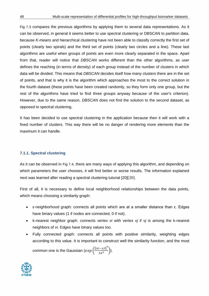
48 Multi-scale representation of differential profiles for high-throughput biomarker datasets
Fig 7.3 compares the previous algorithms by applying them to several data representations. As it
can be observed, in general it seems better to use spectral clustering or DBSCAN to partition data,
because K-means and hierarchical clustering have not been able to classify correctly the first set of
points (clearly two spirals) and the third set of points (clearly two circles and a line). These last
algorithms are useful when groups of points are even more clearly separated in the space. Apart
from that, reader will notice that DBSCAN works different than the other algorithms, as user
defines the reaching (in terms of density) of each group instead of the number of clusters in which
data will be divided. This means that DBSCAN decides itself how many clusters there are in the set
of points, and that is why it is the algorithm which approaches the most to the correct solution in
the fourth dataset (these points have been created randomly, so they form only one group, but the
rest of the algorithms have tried to find three groups anyway because of the user's criterion).
However, due to the same reason, DBSCAN does not find the solution to the second dataset, as
opposed to spectral clustering.
It has been decided to use spectral clustering in the application because then it will work with a
fixed number of clusters. This way there will be no danger of rendering more elements than the
maximum it can handle.
7.1.1. Spectral clustering
As it can be observed in Fig 7.4, there are many ways of applying this algorithm, and depending on
which parameters the user chooses, it will find better or worse results. The information explained
next was learned after reading a spectral clustering tutorial [20][20].
First of all, it is necessary to define local neighborhood relationships between the data points,
which means choosing a similarity graph:
ε-neighborhood graph: connects all points which are at a smaller distance than ε. Edges
have binary values (1 if nodes are connected, 0 if not).
k-nearest neighbor graph: connects vertex vi with vertex vj if vj is among the k-nearest
neighbors of vi. Edges have binary values too.
Fully connected graph: connects all points with positive similarity, weighting edges
according to this value. It is important to construct well the similarity function, and the most
common one is the Gaussian (𝑒𝑥𝑝 (||𝑥𝑖−𝑥𝑗||
2
2𝜎2)).
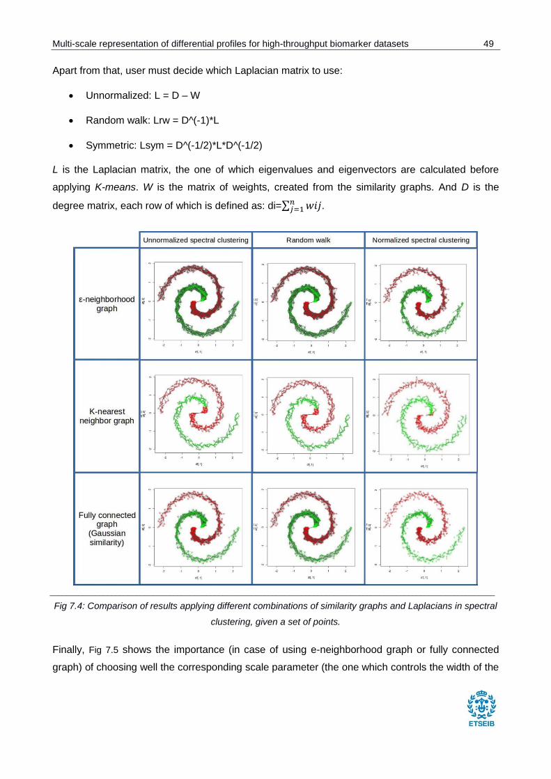
Multi-scale representation of differential profiles for high-throughput biomarker datasets 49
Apart from that, user must decide which Laplacian matrix to use:
Unnormalized: L = D – W
Random walk: Lrw = D^(-1)*L
Symmetric: Lsym = D^(-1/2)*L*D^(-1/2)
L is the Laplacian matrix, the one of which eigenvalues and eigenvectors are calculated before
applying K-means. W is the matrix of weights, created from the similarity graphs. And D is the
degree matrix, each row of which is defined as: di=∑ 𝑤𝑖𝑗𝑛𝑗=1 .
____________________________________________________________________________________________________________
Fig 7.4: Comparison of results applying different combinations of similarity graphs and Laplacians in spectral
clustering, given a set of points.
Finally, Fig 7.5 shows the importance (in case of using e-neighborhood graph or fully connected
graph) of choosing well the corresponding scale parameter (the one which controls the width of the
50 Multi-scale representation of differential profiles for high-throughput biomarker datasets
neighborhoods). It can be observed that:
If the parameter is bigger than its optimal value (or range of values):
◦ The algorithm sets more connections between points, so they join although they are not
part of the same spiral and, therefore, it is more difficult to divide groups correctly.
◦ Time which the algorithm spends to show a solution increases.
◦ In the eigenvectors' graphic (eigenvalues of which are zero) there are not two
completely separated groups. The bigger the scale parameter, the more they approach,
so it is more difficult for the algorithm to apply K-means.
If the parameter is smaller than its optimal value (or range of values):
◦ The algorithm is not capable of identifying all the points which are part of the same
spiral and, therefore, finding two clusters.
◦ In the eigenvectors' graphic (eigenvalues of which are zero) there are more than two
separated groups.
____________________________________________________________________________________________________________
Fig 7.5: Table studying parameter adjustment in spectral clustering using ε-neighborhood similarity graph.
Apart from studying spectral clustering algorithms, many functions have been created during the
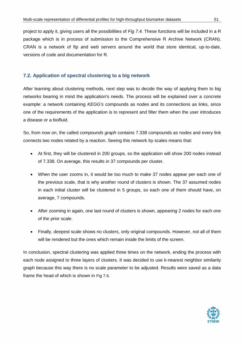
Multi-scale representation of differential profiles for high-throughput biomarker datasets 51
project to apply it, giving users all the possibilities of Fig 7.4. These functions will be included in a R
package which is in process of submission to the Comprehensive R Archive Network (CRAN).
CRAN is a network of ftp and web servers around the world that store identical, up-to-date,
versions of code and documentation for R.
7.2. Application of spectral clustering to a big network
After learning about clustering methods, next step was to decide the way of applying them to big
networks bearing in mind the application's needs. The process will be explained over a concrete
example: a network containing KEGG's compounds as nodes and its connections as links, since
one of the requirements of the application is to represent and filter them when the user introduces
a disease or a biofluid.
So, from now on, the called compounds graph contains 7.338 compounds as nodes and every link
connects two nodes related by a reaction. Seeing this network by scales means that:
At first, they will be clustered in 200 groups, so the application will show 200 nodes instead
of 7.338. On average, this results in 37 compounds per cluster.
When the user zooms in, it would be too much to make 37 nodes appear per each one of
the previous scale, that is why another round of clusters is shown. The 37 assumed nodes
in each initial cluster will be clustered in 5 groups, so each one of them should have, on
average, 7 compounds.
After zooming in again, one last round of clusters is shown, appearing 2 nodes for each one
of the prior scale.
Finally, deepest scale shows no clusters, only original compounds. However, not all of them
will be rendered but the ones which remain inside the limits of the screen.
In conclusion, spectral clustering was applied three times on the network, ending the process with
each node assigned to three layers of clusters. It was decided to use k-nearest neighbor similarity
graph because this way there is no scale parameter to be adjusted. Results were saved as a data
frame the head of which is shown in Fig 7.6.
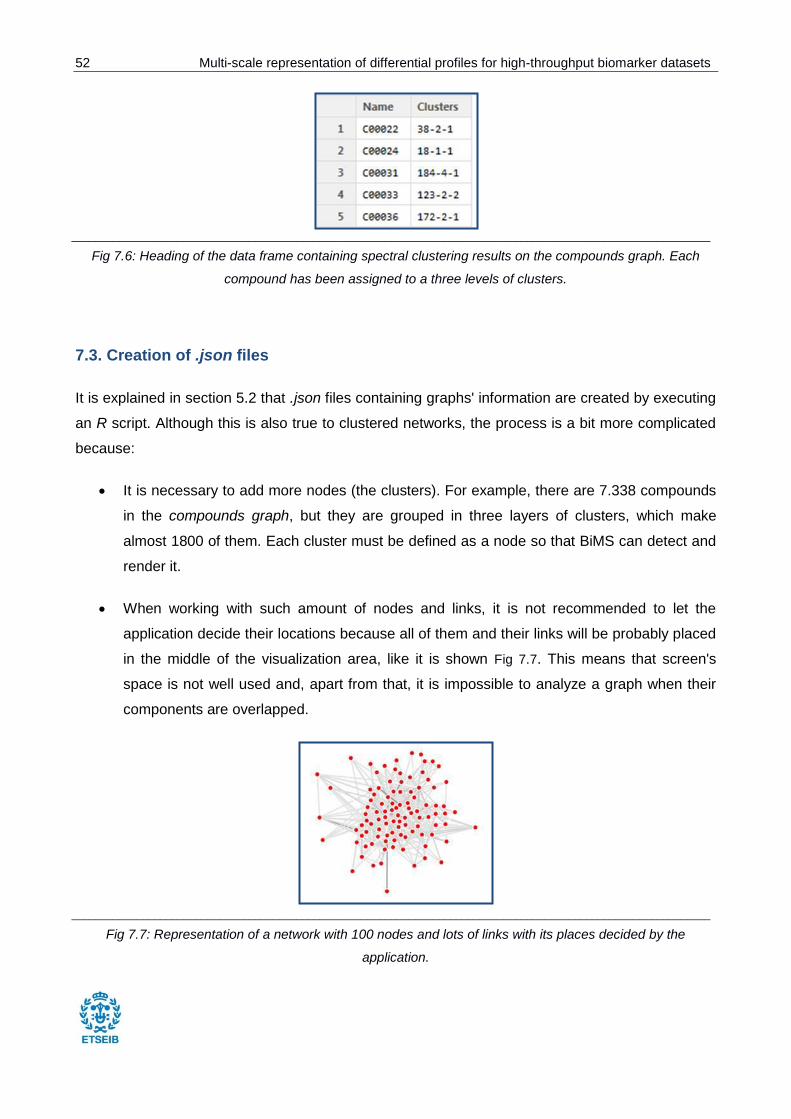
52 Multi-scale representation of differential profiles for high-throughput biomarker datasets
____________________________________________________________________________________________________________
Fig 7.6: Heading of the data frame containing spectral clustering results on the compounds graph. Each
compound has been assigned to a three levels of clusters.
7.3. Creation of .json files
It is explained in section 5.2 that .json files containing graphs' information are created by executing
an R script. Although this is also true to clustered networks, the process is a bit more complicated
because:
It is necessary to add more nodes (the clusters). For example, there are 7.338 compounds
in the compounds graph, but they are grouped in three layers of clusters, which make
almost 1800 of them. Each cluster must be defined as a node so that BiMS can detect and
render it.
When working with such amount of nodes and links, it is not recommended to let the
application decide their locations because all of them and their links will be probably placed
in the middle of the visualization area, like it is shown Fig 7.7. This means that screen's
space is not well used and, apart from that, it is impossible to analyze a graph when their
components are overlapped.
____________________________________________________________________________________________________________
Fig 7.7: Representation of a network with 100 nodes and lots of links with its places decided by the
application.
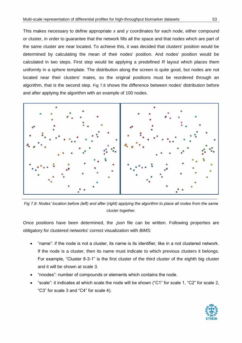
Multi-scale representation of differential profiles for high-throughput biomarker datasets 53
This makes necessary to define appropriate x and y coordinates for each node, either compound
or cluster, in order to guarantee that the network fills all the space and that nodes which are part of
the same cluster are near located. To achieve this, it was decided that clusters' position would be
determined by calculating the mean of their nodes' position. And nodes' position would be
calculated in two steps. First step would be applying a predefined R layout which places them
uniformly in a sphere template. The distribution along the screen is quite good, but nodes are not
located near their clusters' mates, so the original positions must be reordered through an
algorithm, that is the second step. Fig 7.8 shows the difference between nodes' distribution before
and after applying the algorithm with an example of 100 nodes.
____________________________________________________________________________________________________________
Fig 7.8: Nodes’ location before (left) and after (right) applying the algorithm to place all nodes from the same
cluster together.
Once positions have been determined, the .json file can be written. Following properties are
obligatory for clustered networks' correct visualization with BiMS:
“name”: if the node is not a cluster, its name is its identifier, like in a not clustered network.
If the node is a cluster, then its name must indicate to which previous clusters it belongs.
For example, “Cluster 8-3-1” is the first cluster of the third cluster of the eighth big cluster
and it will be shown at scale 3.
“nnodes”: number of compounds or elements which contains the node.
“scale”: it indicates at which scale the node will be shown (“C1” for scale 1, “C2” for scale 2,
“C3” for scale 3 and “C4” for scale 4).
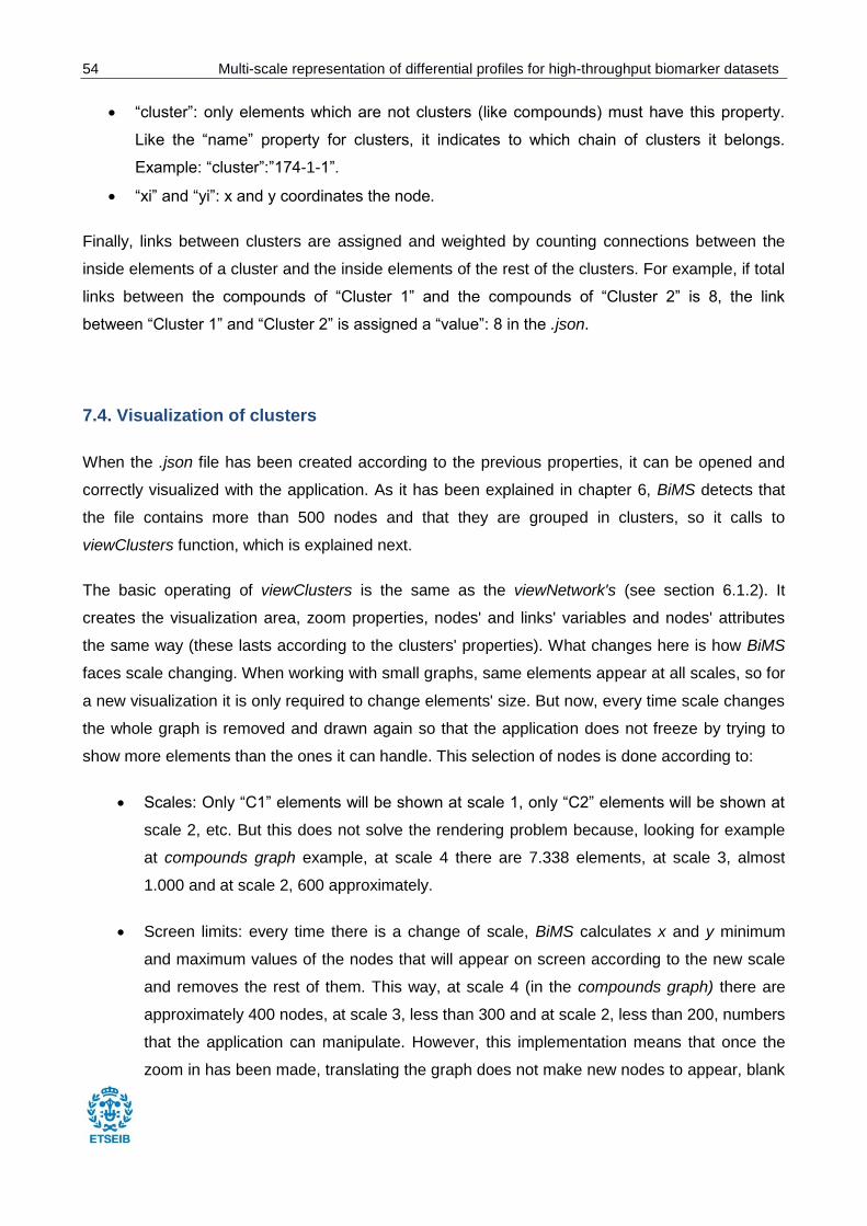
54 Multi-scale representation of differential profiles for high-throughput biomarker datasets
“cluster”: only elements which are not clusters (like compounds) must have this property.
Like the “name” property for clusters, it indicates to which chain of clusters it belongs.
Example: “cluster”:”174-1-1”.
“xi” and “yi”: x and y coordinates the node.
Finally, links between clusters are assigned and weighted by counting connections between the
inside elements of a cluster and the inside elements of the rest of the clusters. For example, if total
links between the compounds of “Cluster 1” and the compounds of “Cluster 2” is 8, the link
between “Cluster 1” and “Cluster 2” is assigned a “value”: 8 in the .json.
7.4. Visualization of clusters
When the .json file has been created according to the previous properties, it can be opened and
correctly visualized with the application. As it has been explained in chapter 6, BiMS detects that
the file contains more than 500 nodes and that they are grouped in clusters, so it calls to
viewClusters function, which is explained next.
The basic operating of viewClusters is the same as the viewNetwork's (see section 6.1.2). It
creates the visualization area, zoom properties, nodes' and links' variables and nodes' attributes
the same way (these lasts according to the clusters' properties). What changes here is how BiMS
faces scale changing. When working with small graphs, same elements appear at all scales, so for
a new visualization it is only required to change elements' size. But now, every time scale changes
the whole graph is removed and drawn again so that the application does not freeze by trying to
show more elements than the ones it can handle. This selection of nodes is done according to:
Scales: Only “C1” elements will be shown at scale 1, only “C2” elements will be shown at
scale 2, etc. But this does not solve the rendering problem because, looking for example
at compounds graph example, at scale 4 there are 7.338 elements, at scale 3, almost
1.000 and at scale 2, 600 approximately.
Screen limits: every time there is a change of scale, BiMS calculates x and y minimum
and maximum values of the nodes that will appear on screen according to the new scale
and removes the rest of them. This way, at scale 4 (in the compounds graph) there are
approximately 400 nodes, at scale 3, less than 300 and at scale 2, less than 200, numbers
that the application can manipulate. However, this implementation means that once the
zoom in has been made, translating the graph does not make new nodes to appear, blank
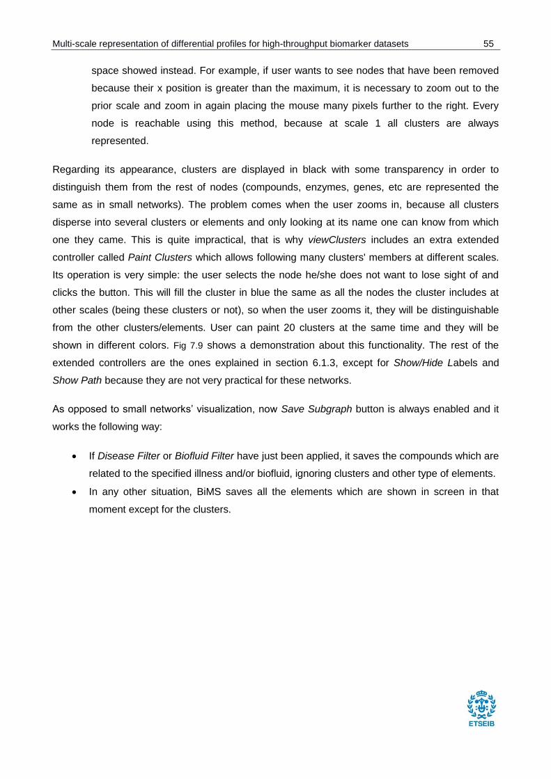
Multi-scale representation of differential profiles for high-throughput biomarker datasets 55
space showed instead. For example, if user wants to see nodes that have been removed
because their x position is greater than the maximum, it is necessary to zoom out to the
prior scale and zoom in again placing the mouse many pixels further to the right. Every
node is reachable using this method, because at scale 1 all clusters are always
represented.
Regarding its appearance, clusters are displayed in black with some transparency in order to
distinguish them from the rest of nodes (compounds, enzymes, genes, etc are represented the
same as in small networks). The problem comes when the user zooms in, because all clusters
disperse into several clusters or elements and only looking at its name one can know from which
one they came. This is quite impractical, that is why viewClusters includes an extra extended
controller called Paint Clusters which allows following many clusters' members at different scales.
Its operation is very simple: the user selects the node he/she does not want to lose sight of and
clicks the button. This will fill the cluster in blue the same as all the nodes the cluster includes at
other scales (being these clusters or not), so when the user zooms it, they will be distinguishable
from the other clusters/elements. User can paint 20 clusters at the same time and they will be
shown in different colors. Fig 7.9 shows a demonstration about this functionality. The rest of the
extended controllers are the ones explained in section 6.1.3, except for Show/Hide Labels and
Show Path because they are not very practical for these networks.
As opposed to small networks’ visualization, now Save Subgraph button is always enabled and it
works the following way:
If Disease Filter or Biofluid Filter have just been applied, it saves the compounds which are
related to the specified illness and/or biofluid, ignoring clusters and other type of elements.
In any other situation, BiMS saves all the elements which are shown in screen in that
moment except for the clusters.
56 Multi-scale representation of differential profiles for high-throughput biomarker datasets
____________________________________________________________________________________________________________
Fig 7.9: Paint Clusters button’s functionality demonstration. Some clusters have been painted at scale 1 (top
left picture) and when zooming in at scale 2 (top right picture), scale 3 (bottom left picture) and scale 4
(bottom right picture), their members are filled in the same color. Pale green nodes are compounds outside
clusters.
Multi-scale representation of differential profiles for high-throughput biomarker datasets 57
8. Integration with R
One of the objectives outlined at the beginning of this project was to allow integrating the final
application with statistical analyses tools. As RStudio is a relevant program for the B2SLab team
(and in bioinformatics in general) and it has been also used during the project for some parts of the
code, this chapter provides a tutorial for including BIMS Viewer in an R package.
Considering a developer who has created many functions which manipulate graphs and make
calculations on them, he/she should include the following commands in the part of the code in
charge of visualizing results:
1. Executing the Rscrip that creates a .json file from an igraph object or from two data frames
containing pathways and genes.
2. Removing last two lines of index2.html and rewriting them. The difference between
index.html and index2.html (see Appendix B for the full code) is that the latter does not
show the welcome screen but directly the graph the user wants to visualize. Although
visualization controllers are no needed for the first representation, they are available in
case other networks are wished to be opened afterwards. In order to make the first graph
to appear when the application starts, index2.html must call to viewNetwork (see chapter
6) passing it the name of the graph, that is why two last lines of this file must be rewritten.
Penultimate line contains this viewNetwork call and last line is </script>.
3. Executing index2.html from R.
Obviously, developer must not forget to include index2.html, plot.js and css folder (these two called
inside index.html) inside his/her R package.
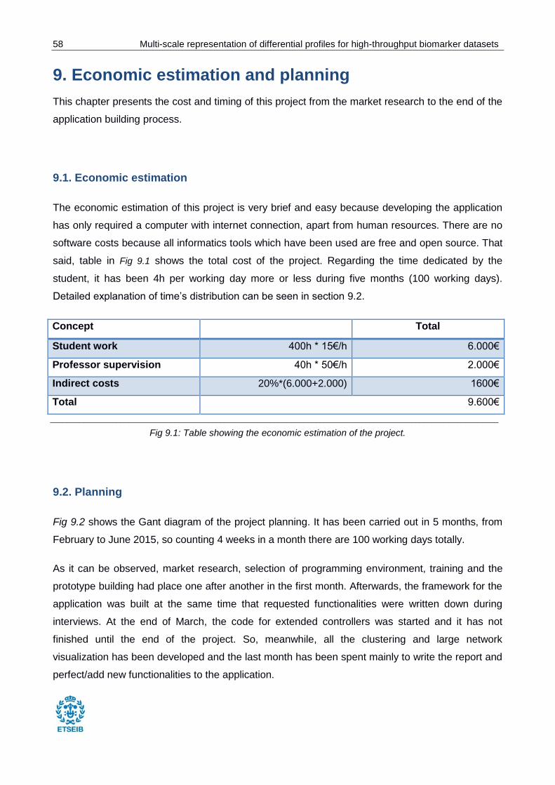
58 Multi-scale representation of differential profiles for high-throughput biomarker datasets
9. Economic estimation and planning
This chapter presents the cost and timing of this project from the market research to the end of the
application building process.
9.1. Economic estimation
The economic estimation of this project is very brief and easy because developing the application
has only required a computer with internet connection, apart from human resources. There are no
software costs because all informatics tools which have been used are free and open source. That
said, table in Fig 9.1 shows the total cost of the project. Regarding the time dedicated by the
student, it has been 4h per working day more or less during five months (100 working days).
Detailed explanation of time’s distribution can be seen in section 9.2.
Concept Total
Student work 400h * 15€/h 6.000€
Professor supervision 40h * 50€/h 2.000€
Indirect costs 20%*(6.000+2.000) 1600€
Total 9.600€
____________________________________________________________________________________________________________
Fig 9.1: Table showing the economic estimation of the project.
9.2. Planning
Fig 9.2 shows the Gant diagram of the project planning. It has been carried out in 5 months, from
February to June 2015, so counting 4 weeks in a month there are 100 working days totally.
As it can be observed, market research, selection of programming environment, training and the
prototype building had place one after another in the first month. Afterwards, the framework for the
application was built at the same time that requested functionalities were written down during
interviews. At the end of March, the code for extended controllers was started and it has not
finished until the end of the project. So, meanwhile, all the clustering and large network
visualization has been developed and the last month has been spent mainly to write the report and
perfect/add new functionalities to the application.
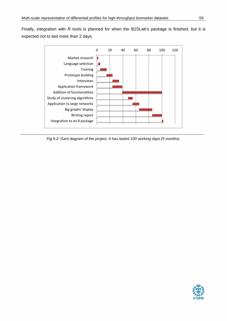
Multi-scale representation of differential profiles for high-throughput biomarker datasets 59
Finally, integration with R tools is planned for when the B2SLab's package is finished, but it is
expected not to last more than 2 days.
____________________________________________________________________________________________________________
Fig 9.2: Gant diagram of the project. It has lasted 100 working days (5 months).
0 20 40 60 80 100 120
Market research
Language selection
Training
Prototype building
Interviews
Application framework
Addition of functionalities
Study of clustering algorithms
Application to large networks
Big graphs' display
Writing report
Integration to an R package
60 Multi-scale representation of differential profiles for high-throughput biomarker datasets
10. Environmental impact
As the product obtained from this project is of software type and it does not generate contaminants
in a direct way, it does not require an exhaustive environmental impact analysis.
The only needed resource to develop it has been a computer, so the basic and unique impact
comes from the electricity it has consumed. Likewise, future users of the application will also need
a computer to make it work, that is why the only impact they will generate is as much electricity as
the time they spend on it. This impact can be reduced by configuring the user device in an energy
saving mode, taking advantage of the new technologies characteristic of the century we live in.
It has not been necessary to use paper during the development of the project because all the tests
and code have been performed on the computer. Apart from that, tutorials and information to
design the application have not been printed but consulted on-line.
Multi-scale representation of differential profiles for high-throughput biomarker datasets 61
Conclusions and further work
At the beginning of the project, a table comparing different characteristics from visualization
programs was made in order to see which line of work would be useful in a new application (see
chapter 2). Now, comparing BiMS with them, it is clear that although this one is not as complete as
the others, it has succeeded on facing the display problem of large networks from its own
perspective. The multi-scale feature joined with the on-line usage generates files smaller than
5MB, while it was said that Cytoscape and other applications require 2GB in the user’s computer.
Considering the time spent in developing this project and the lack of previous knowledge about the
tools used, results are quite satisfactory. Not all of the interviewees’ requests were achieved but
they did the most important ones, as well as all the objectives proposed at the beginning of the
project. Besides, BiMS is simple to understand and use, which is a nice characteristic for new
users, so this project could be the first step to launch a more complete application. This could be
updated every certain time adding statistical analysis, graphics and more information of public
databases, always counting with the assessment of experts in the biological field.
At a personal level, this project has allowed not only going deep in programming languages but
also learning both statistical methods and biological concepts at the same time, so it has been a
really complete and good experience.
Regarding further work, it is recommendable to focus in the following three points, as they would
make the application powerful enough to offer a similar service as the ones described:
Binding the application with an RStudio on-line environment. This would allow, among other
things, widen available entering formats for networks, doing all the clustering calculations
inside BiMS and performing lots of statistical analysis, since RStudio is a very complete tool
in this field.
Implementing the remaining functionalities requested by interviewees.
Including more information about HMDB and KEGG and getting information about more
databases, since this line is being followed by most of this type of applications the present
day, especially Cytoscape.
62 Multi-scale representation of differential profiles for high-throughput biomarker datasets
Bibliography
[1] OGATA, H., GOTO, S., SATO, K., FUJIBUCHI, W., BONO, H., KANEHISA, M.; KEGG:
Kyoto Encyclopedia of Genes and Genomes. Nucleic Acids Res. 27, 29-34 (1999)
[2] JOSHI-TOPE, G [et al]. Reactome: a knowledgebase of biological pathways. Nucleic acids
research (2005)
[3] WISHART DS, TZUR D, KNOX C [et al.], HMDB: the Human Metabolome Database.
Nucleic Acids Res. (January 2007)
[4] DAVISS, Bennett. Growing pains for metabolomics. The Scientist (April 2005)
[5] MADAN BABU M., An Introduction to Microarray Data Analysis.
[6] ASHBURNER [et al]. Gene ontology: tool for the unification of biology (2000)
[7] RSTUDIO INC. RStudio web site. [http://www.rstudio.com/, February 2015]
[8] Gentleman [et al]., Genome Biology 5:R80 (2004)
[9] SHANNON P [et al]. Cytoscape: a software environment for integrated models of
biomolecular interaction networks. Genome Research 2003 Nov; 13(11):2498-504
[10] QIAGEN REDWOOD CITY. INGENUITY Pathway Analysis web site.
[http://www.ingenuity.com/products/ipa, February 2015]
[11] BIK, H.M., BU, S., GRUBBS, W. (manuscript in preparation). Phinch: An interactive,
exploratory data visualization framework for environnmental sequence data.
[https://github.com/PitchInteractiveInc/Phinch, February 2015]
[12] WRIGHT D.W., ANGUS T., ENRIGHT A.J., FREEMAN T.C. Visualisation of BioPAX
Networks using BioLayout Express3D F1000Research. 2014, 3:246 (doi:
10.12688/f1000research.5499.1).
[13] BREITKREUTZ, BOBBY-JOE, STARK, CHRIS, TYERS, MIKE. Osprey: a network
visualization system. Genome Biology 2003, 4:R22
[14] DROSTE, Peter; NÖH, Katharina; WIECHERT, Wolfgang. Omix – A Visualization Tool
for Metabolic Networks with Highest Usability and Customizability in Focus. Chemie
Ingenieur Technik 2013, 85, 6, 849–862
[15] BOSTOCK, MIKE. D3 web site. [http://d3js.org/, February 2015]
[16] RSTUDIO INC. Shiny web site. [http://shiny.rstudio.com/]
[17] VAIDYANATHAN, RAMNATH, RUSSELL, KENGTON, RSTUDIO INC. Htmlwidgets web
site. [http://www.htmlwidgets.org/, February 2015]
[18] GANDRUD, CHRISTOPHER, ALLAIRE JJ. NetworkD3: D3 JavaScript Network Graphs
from R. v0.1.3

Multi-scale representation of differential profiles for high-throughput biomarker datasets 63
[19] MACLEAN, MALCOLM. D3 Tips and Tricks, Interactive Data Visualization in a Web
Browser. 2013 March.
[20] VON LUXBURG, ULRIKE. A Tutorial on Spectral Clustering. Statistics and Computing,
17(4):395{416, dec 2007.
64 Multi-scale representation of differential profiles for high-throughput biomarker datasets
A. Interviews
In this section, reader will find the interviews which took place to get specific requirements for the
application. In the first one, the interviewee is a researcher in bioinformatics; in the second one, a
researcher in biomedical data analysis; and in the last one, a biochemist.
A.1. Interview 1
First interviewee is Sergi Picart, researcher in bioinformatics and member of B2SLab.
1. Which options and functionalities would you like this application to have?
I would like to see nodes’ names as labels permanently instead of only when the mouse is over
them because otherwise it is tiresome to know what each node is representing. Even better if
there is a button which allows labels to appear and disappear. I would also like to see a
description of a node when I click on it and it would be really useful to go to KEGG's URL
address of a node when I double click on it. Basically, what I want is to make this graph as
interactive as possible: making nodes appear and disappear, saving subgraphs, making
annotations, painting lost connections... A button allowing searching for a node would be very
useful too. And do nodes have always these colors? I would like to change them for the ones I
am used to. If you want I can tell you more functionalities, but I think it would be better if you let
me try a new version of the application after Easter and then we talk again.
2. In which format do you have the data to enter to the application?
I usually work with the igraph package (of Rstudio), so I have graphs as igraph objects. I can
convert them to whichever format you need or I can share them as RData objects (in this case I
will also give you two .pdf files containing useful information about igraph). I will send you an e-
mail with these objects and I will include URL address to which I would like to go when double
clicking a node. As for nodes’ descriptions, I think I have them as RData objects too
(dataframes), I will include them on the e-mail.
3. Which program are you using at the moment to display data and why does it not meet
your needs?
I am using a Shiny application of my own which allows me to make different calculations and
analysis over a graph. It also generates .pdf files with results. Networks are represented as
static images and I usually print them to make annotations, painting lost connections, etc. It
would be really useful to study them on the computer instead of by hand, that is why I have
Multi-scale representation of differential profiles for high-throughput biomarker datasets 65
asked for the interactivity features in your application.
A2. Interview 2
Second interviewee is Maria Maqueda, researcher in biomedical data analysis and also member of
B2SLab.
1. Which options and functionalities would you like this application to have?
I already like this display, especially the part of moving nodes, but it lacks labels with their
names on top or bottom of each one. I would also like to see at first only pathways with their full
name (not their ID), when you zoom in I would like to see genes too (colored according to their
fold change value) and then to have all labels with ID's instead of full names. A button or
something which allows user to change the color of nodes would be very useful too. And you
could try another type of representations, like sunburst (significant pathways are placed in a
circle inside of which you have their connections according to the genes they have in common.
Genes are not displayed), hypertree (you could represent all existent pathways and color only
significant ones in the current analysis. The information about pathways and their connections
can be extracted from Reactome) or treemap (this visualization would be useful for GO, it draws
squares grouped by categories). There are several demos about all of these representations in
JavasScrip InfoVis Toolkit, if you want to look at them.
2. In which format do you have the data to enter to the application?
I have two .csv files. The first one contains a table with these columns: pathways’ ID, pathways’
description, gene ratio, bg ratio, pvalue, p adjust, qvalue and the genes related to each
pathway. The second one contains a table with each gene next to its fold change value. I can
copy in your USB device an example of each one so you can work with them.
3. Which program are you using at the moment to display data and why does it not meet
your needs?
Well, first let me say that it is not obligatory to represent results in form of a network, there are
scientists who get the list or table of genes and publish this as the final result. However, I think
results are clearer when you display them. At the moment I am using an R package called
clusterProfile, basically to work with KEGG PATHWAY and Reactome because this package
calls at these databases. Inside this package there is a function called enrichMap (see Fig 4.2),
which shows the existing pathways relations (through genes, these not shown), but its graph
representation is not totally clear from my point of view. One option is to download the code of
66 Multi-scale representation of differential profiles for high-throughput biomarker datasets
the package and modify it, but this means a lot of work. I also use another function called
cnetplot (from another package) which makes better representations: it displays genes around
pathways, and every gene has a color according to its fold change value (greenish for negative
values and reddish for the positive). Graphics are okay when using this function, but there is a
mess of lines and letters and it is tiresome to clear them up with pdf tool, which is what I do.
A.3. Interview 3
Third interviewee is Oscar Yanes, Ph.D. Co-ordinator of the Metabolomics Platform of the Spanish
Biomedical Research Centre in Diabetes and Associated Metabolic Disorders (CIBERDEM) and
Assistant Professor at the Rovira i Virgili University (Tarragona, Spain). He also collaborates with
B2SLab.
1. Which options and functionalities would you like this application to have?
I like Cytoscape’s networks representation, so it would be quite good if your application got to
display graphs the same way. I cannot think of extra functionalities to be added in terms of
visualization, for the moment. However, as you will work with KEGG database, it would be really
useful to apply filters to its metabolites in order to find, for example, which ones are related to
cancer or other diseases. These illnesses' information can be extracted from the Human
Database. If you go to its web site, you will see that every metabolite has a document called
MetaboCard with lots of information (there are like 60000 of them) and that is why it is not
feasible to look one by one. Most of metabolites of the Human Database have a KEGG
identifier, so what I would like you to do is to display KEGG and light up metabolites which are
involved with the disease I write. Apart from that, I would like to filter metabolites by the biofluids
where they are located (blood, urine, etc) and to combine disease and biofluid filter so that I can
ask the application to color nodes which have to do with cancer in blood, for example. Finally,
mass information is also very interesting: you can use the value mono_mass (the neutral value
of the metabolite) as an input to build a network and then use other criterion to prioritize or
enrich the best graph option. Every mass can have several hits in databases and this would be
a way to analyze LC-MS data. There are already some papers pointing at this direction, but they
do not use all the possibilities that MetaboCards can offer.
2. In which format do you have the data to enter to the application?
Well, for the features I have asked you to represent I have not a specific data format. You are
already working with KEGG, so display it with the data you are using at the moment. And as for
the MetaboCards, they are available at HMDB website, you can extract the information from

Multi-scale representation of differential profiles for high-throughput biomarker datasets 67
there.
3. Which program are you using at the moment to display data and why does it not meet
your needs?
I mainly use Cytoscape to display biological networks, especially one of its plugins called
MetScape, which allows representing compound networks. As I have told you before, its
visualizations are really good. In fact, I do not really know its real potential because I have only
used a little part of the program. But it does not have the filters part, so that would be an
interesting step for your application.
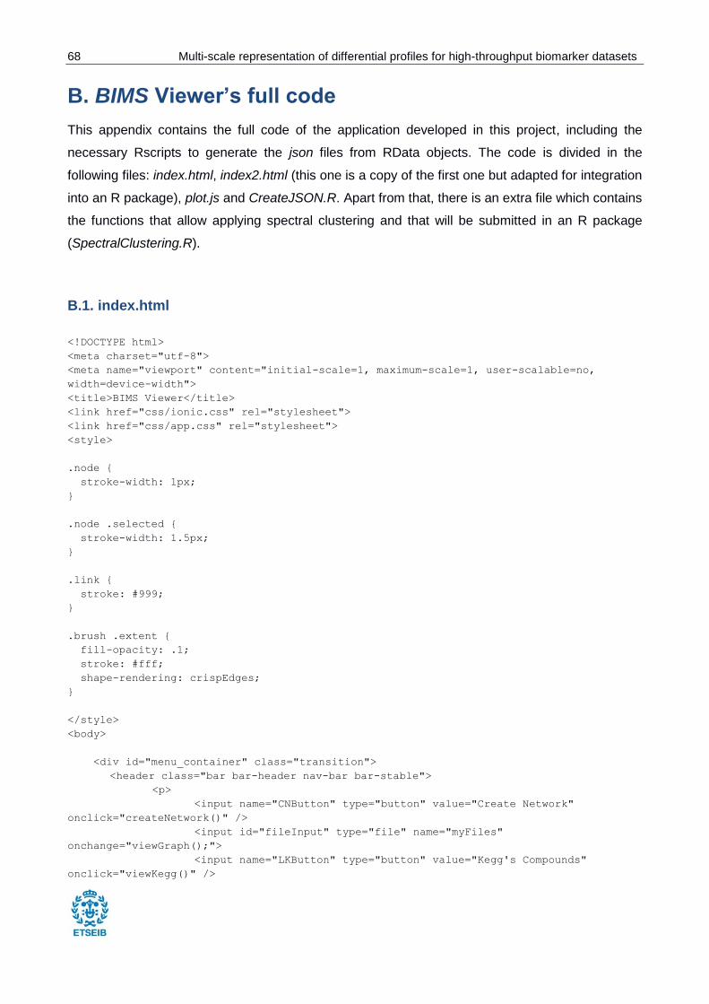
68 Multi-scale representation of differential profiles for high-throughput biomarker datasets
B. BIMS Viewer’s full code
This appendix contains the full code of the application developed in this project, including the
necessary Rscripts to generate the json files from RData objects. The code is divided in the
following files: index.html, index2.html (this one is a copy of the first one but adapted for integration
into an R package), plot.js and CreateJSON.R. Apart from that, there is an extra file which contains
the functions that allow applying spectral clustering and that will be submitted in an R package
(SpectralClustering.R).
B.1. index.html
<!DOCTYPE html>
<meta charset="utf-8">
<meta name="viewport" content="initial-scale=1, maximum-scale=1, user-scalable=no,
width=device-width">
<title>BIMS Viewer</title>
<link href="css/ionic.css" rel="stylesheet">
<link href="css/app.css" rel="stylesheet">
<style>
.node {
stroke-width: 1px;
}
.node .selected {
stroke-width: 1.5px;
}
.link {
stroke: #999;
}
.brush .extent {
fill-opacity: .1;
stroke: #fff;
shape-rendering: crispEdges;
}
</style>
<body>
<div id="menu_container" class="transition">
<header class="bar bar-header nav-bar bar-stable">
<p>
<input name="CNButton" type="button" value="Create Network"
onclick="createNetwork()" />
<input id="fileInput" type="file" name="myFiles"
onchange="viewGraph();">
<input name="LKButton" type="button" value="Kegg's Compounds"
onclick="viewKegg()" />
Multi-scale representation of differential profiles for high-throughput biomarker datasets 69
</p>
</header>
</div>
<div align='center' id="d3_graph"></div>
<script src="http://d3js.org/d3.v3.min.js"></script>
<script src="plot.js"></script>
<script src="js/app.js"></script>
<script>
var width = window.innerWidth,
height = window.innerHeight,
shiftKey, ctrlKey;
var svg = d3.select("body").append("svg")
.attr("width", width)
.attr("height", height)
d3.selectAll('svg')
.append('image')
.attr('xlink:href','wscreen.png')
.attr('class', 'pico')
.attr('height', height)
.attr('width', width)
.attr('x', 0)
.attr('y', 0)
function createNetwork() {
filtered = window.prompt("Please, insert min/max mass values (m) or a single value
to create the network.\n","150/1000")
//el valor mínimo para que haya un nodo es 1.007825 y el máximo es 6176.018
var minim = 1.007825
var maxim = 6176.018
var coma = true
while (coma) {
ind = filtered.indexOf(",")
if (ind!=-1) {filtered[ind] = "."}
else {coma=false}
}
filtered = filtered.split("/")
if (filtered.length==1) {
filtn = Number(filtered[0])
if (isNaN(filtn)) {
minim = 0
alert('"'+filtered[0]+'" is a word, not a number."')
}
else if (filtn<minim && filtn>maxim) {
minim = 0
maxim = 7000
alert("Minimum and maximum allowed values are 1.007825 and
6176.018.")
}
else if (filtn<minim) {
minim = 0
alert("Minimum allowed value is 1.007825.")
}
else if (filtn>maxim) {
70 Multi-scale representation of differential profiles for high-throughput biomarker datasets
maxim = 7000
alert("Maximum allowed value is 6176.018.")
}
else {
minim = filtn
maxim = filtn
}
}
else if (filtered.length==2) {
filt1 = Number(filtered[0])
filt2 = Number(filtered[1])
if (isNaN(filt1) && isNaN(filt2)) {
minim = 0
alert('"'+filtered[0]+'" and "'+filtered[1]+'" are words, not
numbers."')
}
else if (isNaN(filt1)) {
minim = 0
alert('"'+filtered[0]+'" is a word, not a number."')
}
else if (isNaN(filt2)) {
minim = 0
alert('"'+filtered[1]+'" is a word, not a number."')
}
else if (filt1>filt2) {
aux = filt1
filt1 = filt2
filt2 = aux
}
if (filt1<minim && filt2>maxim) {
minim = 0
maxim = 7000
alert("Minimum and maximum allowed values are 1.007825 and
6176.018.")
}
else if (filt1<minim) {
minim = 0
alert("Minimum allowed value is 1.007825.")
}
else if (filt2>maxim) {
maxim = 7000
alert("Maximum allowed value is 6176.018.")
}
else {
minim = filt1
maxim = filt2
}
}
else {
minim = 0
alert("Only one or two values required, not "+filtered.length+".")
}
if (minim>=1.007825 && maxim<=61676.018) {
d3.select("svg").remove();
d3.selectAll("button").remove()
//alert(minim)
//selectableForceDirectedGraph("comp26.json",minim,maxim)}
Multi-scale representation of differential profiles for high-throughput biomarker datasets 71
var nData = new Array();
var mm = new Array();
var conc = new Array();
d3.json("comp29.json", function(error, graph) {
graph.nodes.forEach(function(d) {
if (d.name.substring(0,7)!="Cluster" && d.group=="Compound")
{nData.push(d.name);mm.push(d.name);conc.push(0)}
})
})
setTimeout(function(){//alert(nData.length); }, 40);
//function fillnData () {
//alert(nData.length)
//}
//alert(nData.length)
d3.csv("index-hmdb.csv",function(d) {
return {
kegg_id: d.kegg_id,
path: d.path
};
}, function(error,rows) {
rows.forEach(function(h) {
//alert(nData.indexOf(h.kegg_id))
if (nData.indexOf(h.kegg_id)!=-1) {
d3.xml(h.path,function(xml) {
mm[nData.indexOf(h.kegg_id)] =
xml.documentElement.getElementsByTagName("predicted_properties")
var string =
[].map.call( mm[nData.indexOf(h.kegg_id)], function(dnode){
conc[nData.indexOf(h.kegg_id)] =
dnode.textContent || dnode.innerText || ""
//alert(conc)
conc[nData.indexOf(h.kegg_id)] =
conc[nData.indexOf(h.kegg_id)].split("mono_mass")
//alert(mm2)
conc[nData.indexOf(h.kegg_id)] =
conc[nData.indexOf(h.kegg_id)][1].split("ChemAxon")
conc[nData.indexOf(h.kegg_id)] =
Number(conc[nData.indexOf(h.kegg_id)][0])
//alert(mm4)
if (h.kegg_id=="C00334") {
alert(minim+"
"+conc[nData.indexOf(h.kegg_id)]+" "+maxim)
alert(conc[nData.indexOf(h.kegg_id)]>minim)
alert(conc[nData.indexOf(h.kegg_id)]<maxim)
alert(minim+"
"+conc[nData.indexOf(h.kegg_id)]+" "+maxim)
//alert(typeof(mm4))
//alert(typeof(minim))
}
if
(conc[nData.indexOf(h.kegg_id)]>=minim && conc[nData.indexOf(h.kegg_id)]<=maxim) { return
"yes" }; }).join("")
if (string=="")
{ nData.splice(nData.indexOf(h.kegg_id),1)}
})
72 Multi-scale representation of differential profiles for high-throughput biomarker datasets
}
})
})
setTimeout(function(){alert(conc);alert(nData.indexOf("C00334"));alert(nData.lengt
h)},5000)
},4000)
//while (i<graph.nodes.length) {
// igfound = false
// h = rows.getElementById(graph.nodes[i].name)
// alert(h.kegg_id)
// i = i+1
//}
//alert(nData)
}
}
function viewGraph() {
var fileSelected = document.getElementById("fileInput").files,
fileFormat = fileSelected[0].name.substring(fileSelected[0].name.length-5)
if (fileFormat==".json") {
d3.select("svg").remove();
d3.selectAll("button").remove()
d3.json(fileSelected[0].name, function(error, graph) {
if (graph.nodes.length<500) { viewNetwork(fileSelected[0].name,"") }
else {viewClusters(fileSelected[0].name)}
})
}
else {alert("Please, select a '.json' file.");}
}
function viewKegg() {
d3.select("svg").remove();
d3.selectAll("button").remove()
viewClusters("comp29.json")
}
function selectableForceDirectedGraph(fileSelected,minim,maxim) {
d3.select("svg").remove();
d3.selectAll("button").remove()
//d3.json(fileSelected, function(error, graph) {
//alert("1")
//alert(graph.nodes.length)
if (minim!="" && maxim!="") {
var nData = new Array();
//alert("2")
//dataAsNodes = graph.nodes.filter(isBetweenMM)
//function isBetweenMM(element) {return element}
//alert(dataAsNodes.length)
//alert("5")
//var yes = false
//alert(element.group)
//if (element.group=="Compound"){
//alert("4")
d3.csv("index-hmdb.csv",function(d) {
alert("3")
return {
Multi-scale representation of differential profiles for high-throughput biomarker datasets 73
kegg_id: d.kegg_id,
path: d.path
};
}, function(error,rows) {
i = 0
//alert("7")
while (i<graph.nodes.length) {
//alert("6")
igfound = false
rows.forEach(function(h) {
//alert("8")
if (!igfound) {
if (graph.nodes[i].name==h.kegg_id) {
igfound = true
//alert("9")
d3.xml(h.path,function(xml) {
mm =
xml.documentElement.getElementsByTagName("predicted_properties")
//alert(mm)
var string = [].map.call( mm, function(dnode){
var conc = dnode.textContent
|| dnode.innerText || ""
//alert(conc)
mm2 = conc.split("mono_mass")
//alert(mm2)
mm3 = mm2[1].split("ChemAxon")
mm4 = Number(mm3[0])
//alert(mm4)
if (mm4>=minim &&
mm4<=maxim) { return "yes" }; }).join("")
if (string!="") { nData.push(graph.nodes[i]) }
})
}
}
})
i = i+1
}
})
alert(nData.length)
window.setTimeout(setData,15000)
function setData() {alert(nData.length)}
//if (yes) {return element}
// }
//}
//alert("3")
//if (dataAsNodes.length<500) {
//alert(dataAsNodes)
//viewNetwork(fileSelected,dataAsNodes)
//}
//else {alert("Too many compounds to draw. Please select a smaller range of
values.")}
}
//else {
//if (graph.nodes.length<500) { viewNetwork(fileSelected,"") }
//else {viewClusters(fileSelected)}
//}
//})
74 Multi-scale representation of differential profiles for high-throughput biomarker datasets
}
</script>
B.2. index2.html
<!DOCTYPE html>
<meta charset="utf-8">
<meta name="viewport" content="initial-scale=1, maximum-scale=1, user-scalable=no,
width=device-width">
<title>BIMS Viewer</title>
<link href="css/ionic.css" rel="stylesheet">
<link href="css/app.css" rel="stylesheet">
<style>
.node {
stroke-width: 1px;
}
.node .selected {
stroke-width: 1.5px;
}
.link {
stroke: #999;
}
.brush .extent {
fill-opacity: .1;
stroke: #fff;
shape-rendering: crispEdges;
}
</style>
<body>
<div id="menu_container" class="transition">
<header class="bar bar-header nav-bar bar-stable">
<p>
<input name="CNButton" type="button" value="Create Network"
onclick="createNetwork()" />
<input id="fileInput" type="file" name="myFiles"
onchange="viewGraph();">
<input name="LKButton" type="button" value="Kegg's Compounds"
onclick="viewKegg()" />
</p>
</header>
</div>
<div align='center' id="d3_graph"></div>
<script src="http://d3js.org/d3.v3.min.js"></script>
<script src="plot.js"></script>
<script src="js/app.js"></script>
<script>
Multi-scale representation of differential profiles for high-throughput biomarker datasets 75
function createNetwork() {
filtered = window.prompt("Please, insert min/max mass values (m) or a single value
to create the network.\n","150/1000")
//el valor mínimo para que haya un nodo es 1.007825 y el máximo es 6176.018
var minim = 1.007825
var maxim = 6176.018
var coma = true
while (coma) {
ind = filtered.indexOf(",")
if (ind!=-1) {filtered[ind] = "."}
else {coma=false}
}
filtered = filtered.split("/")
if (filtered.length==1) {
filtn = Number(filtered[0])
if (isNaN(filtn)) {
minim = 0
alert('"'+filtered[0]+'" is a word, not a number."')
}
else if (filtn<minim && filtn>maxim) {
minim = 0
maxim = 7000
alert("Minimum and maximum allowed values are 1.007825 and
6176.018.")
}
else if (filtn<minim) {
minim = 0
alert("Minimum allowed value is 1.007825.")
}
else if (filtn>maxim) {
maxim = 7000
alert("Maximum allowed value is 6176.018.")
}
else {
minim = filtn
maxim = filtn
}
}
else if (filtered.length==2) {
filt1 = Number(filtered[0])
filt2 = Number(filtered[1])
if (isNaN(filt1) && isNaN(filt2)) {
minim = 0
alert('"'+filtered[0]+'" and "'+filtered[1]+'" are words, not
numbers."')
}
else if (isNaN(filt1)) {
minim = 0
alert('"'+filtered[0]+'" is a word, not a number."')
}
else if (isNaN(filt2)) {
minim = 0
alert('"'+filtered[1]+'" is a word, not a number."')
}
else if (filt1>filt2) {
aux = filt1
filt1 = filt2
76 Multi-scale representation of differential profiles for high-throughput biomarker datasets
filt2 = aux
}
if (filt1<minim && filt2>maxim) {
minim = 0
maxim = 7000
alert("Minimum and maximum allowed values are 1.007825 and
6176.018.")
}
else if (filt1<minim) {
minim = 0
alert("Minimum allowed value is 1.007825.")
}
else if (filt2>maxim) {
maxim = 7000
alert("Maximum allowed value is 6176.018.")
}
else {
minim = filt1
maxim = filt2
}
}
else {
minim = 0
alert("Only one or two values required, not "+filtered.length+".")
}
if (minim>=1.007825 && maxim<=61676.018) {
d3.select("svg").remove();
d3.selectAll("button").remove()
//alert(minim)
//selectableForceDirectedGraph("comp26.json",minim,maxim)}
var nData = new Array();
var mm = new Array();
var conc = new Array();
d3.json("comp29.json", function(error, graph) {
graph.nodes.forEach(function(d) {
if (d.name.substring(0,7)!="Cluster" && d.group=="Compound")
{nData.push(d.name);mm.push(d.name);conc.push(0)}
})
})
setTimeout(function(){//alert(nData.length); }, 40);
//function fillnData () {
//alert(nData.length)
//}
//alert(nData.length)
d3.csv("index-hmdb.csv",function(d) {
return {
kegg_id: d.kegg_id,
path: d.path
};
}, function(error,rows) {
rows.forEach(function(h) {
//alert(nData.indexOf(h.kegg_id))
if (nData.indexOf(h.kegg_id)!=-1) {
d3.xml(h.path,function(xml) {
mm[nData.indexOf(h.kegg_id)] =
xml.documentElement.getElementsByTagName("predicted_properties")
var string =
Multi-scale representation of differential profiles for high-throughput biomarker datasets 77
[].map.call( mm[nData.indexOf(h.kegg_id)], function(dnode){
conc[nData.indexOf(h.kegg_id)] =
dnode.textContent || dnode.innerText || ""
//alert(conc)
conc[nData.indexOf(h.kegg_id)] =
conc[nData.indexOf(h.kegg_id)].split("mono_mass")
//alert(mm2)
conc[nData.indexOf(h.kegg_id)] =
conc[nData.indexOf(h.kegg_id)][1].split("ChemAxon")
conc[nData.indexOf(h.kegg_id)] =
Number(conc[nData.indexOf(h.kegg_id)][0])
//alert(mm4)
if (h.kegg_id=="C00334") {
alert(minim+"
"+conc[nData.indexOf(h.kegg_id)]+" "+maxim)
alert(conc[nData.indexOf(h.kegg_id)]>minim)
alert(conc[nData.indexOf(h.kegg_id)]<maxim)
alert(minim+"
"+conc[nData.indexOf(h.kegg_id)]+" "+maxim)
//alert(typeof(mm4))
//alert(typeof(minim))
}
if
(conc[nData.indexOf(h.kegg_id)]>=minim && conc[nData.indexOf(h.kegg_id)]<=maxim) { return
"yes" }; }).join("")
if (string=="")
{ nData.splice(nData.indexOf(h.kegg_id),1)}
})
}
})
})
setTimeout(function(){alert(conc);alert(nData.indexOf("C00334"));alert(nData.lengt
h)},5000)
},4000)
//while (i<graph.nodes.length) {
// igfound = false
// h = rows.getElementById(graph.nodes[i].name)
// alert(h.kegg_id)
// i = i+1
//}
//alert(nData)
}
}
function viewGraph() {
var fileSelected = document.getElementById("fileInput").files,
fileFormat = fileSelected[0].name.substring(fileSelected[0].name.length-5)
if (fileFormat==".json") {
d3.select("svg").remove();
d3.selectAll("button").remove()
d3.json(fileSelected[0].name, function(error, graph) {
if (graph.nodes.length<500) { viewNetwork(fileSelected[0].name,"") }
else {viewClusters(fileSelected[0].name)}
})
78 Multi-scale representation of differential profiles for high-throughput biomarker datasets
}
else {alert("Please, select a '.json' file.");}
}
function viewKegg() {
d3.select("svg").remove();
d3.selectAll("button").remove()
viewClusters("comp29.json")
}
function selectableForceDirectedGraph(fileSelected,minim,maxim) {
d3.select("svg").remove();
d3.selectAll("button").remove()
//d3.json(fileSelected, function(error, graph) {
//alert("1")
//alert(graph.nodes.length)
if (minim!="" && maxim!="") {
var nData = new Array();
//alert("2")
//dataAsNodes = graph.nodes.filter(isBetweenMM)
//function isBetweenMM(element) {return element}
//alert(dataAsNodes.length)
//alert("5")
//var yes = false
//alert(element.group)
//if (element.group=="Compound"){
//alert("4")
d3.csv("index-hmdb.csv",function(d) {
alert("3")
return {
kegg_id: d.kegg_id,
path: d.path
};
}, function(error,rows) {
i = 0
//alert("7")
while (i<graph.nodes.length) {
//alert("6")
igfound = false
rows.forEach(function(h) {
//alert("8")
if (!igfound) {
if (graph.nodes[i].name==h.kegg_id) {
igfound = true
//alert("9")
d3.xml(h.path,function(xml) {
mm =
xml.documentElement.getElementsByTagName("predicted_properties")
//alert(mm)
var string = [].map.call( mm, function(dnode){
var conc = dnode.textContent
|| dnode.innerText || ""
//alert(conc)
mm2 = conc.split("mono_mass")
//alert(mm2)
mm3 = mm2[1].split("ChemAxon")
mm4 = Number(mm3[0])
Multi-scale representation of differential profiles for high-throughput biomarker datasets 79
//alert(mm4)
if (mm4>=minim &&
mm4<=maxim) { return "yes" }; }).join("")
if (string!="") { nData.push(graph.nodes[i]) }
})
}
}
})
i = i+1
}
})
alert(nData.length)
window.setTimeout(setData,15000)
function setData() {alert(nData.length)}
//if (yes) {return element}
// }
//}
//alert("3")
//if (dataAsNodes.length<500) {
//alert(dataAsNodes)
//viewNetwork(fileSelected,dataAsNodes)
//}
//else {alert("Too many compounds to draw. Please select a smaller range of
values.")}
}
//else {
//if (graph.nodes.length<500) { viewNetwork(fileSelected,"") }
//else {viewClusters(fileSelected)}
//}
//})
}
viewNetwork(“TestGraphData.json”,””)
</script>
B.3. plot.js
function viewNetwork(fileToView,massData,massValues) {
var width = window.innerWidth,
height = window.innerHeight-35,
shiftKey, ctrlKey;
var nodeGraph = null;
var vnodeGraph = null;
var xScale = d3.scale.linear()
.domain([0,width]).range([0,width]);
var yScale = d3.scale.linear()
.domain([0,height]).range([0, height]);
var divButtons = d3.select("body").append("div")
.style("width", width)
.style("height", 100)
.attr("id","extendedC")
var svg = d3.select("#d3_graph")
.attr("tabindex", 1)
80 Multi-scale representation of differential profiles for high-throughput biomarker datasets
.on("keydown.brush", keydown)
.on("keyup.brush", keyup)
.each(function() { this.focus(); })
.append("svg")
.attr("width", width)
.attr("height", height);
var zoomer = d3.behavior.zoom().
scaleExtent([0.1,100]).
x(xScale).
y(yScale).
on("zoomstart", zoomstart).
on("zoom", redraw);
function zoomstart() {
node.each(function(d) {
d.selected = false;
d.previouslySelected = false;
});
node.classed("selected", false);
node.style("stroke-width",1)
node.classed("fixed", function(d) { d.fixed = true; });
}
function redraw() {
vis.attr("transform",
"translate(" + d3.event.translate + ")" + " scale(" + d3.event.scale +
")");
}
var brusher = d3.svg.brush()
.x(xScale)
.y(yScale)
.on("brushstart", function(d) {
node.each(function(d) {
d.previouslySelected = shiftKey && d.selected; });
})
.on("brush", function() {
var extent = d3.event.target.extent();
node.classed("selected", function(d) {
return d.selected = d.previouslySelected ^
(extent[0][0] <= d.x && d.x < extent[1][0]
&& extent[0][1] <= d.y && d.y < extent[1][1]);
});
})
.on("brushend", function() {
d3.event.target.clear();
d3.select(this).call(d3.event.target);
});
var svg_graph = svg.append('svg:g')
.call(zoomer)
var rect = svg_graph.append('svg:rect')
.attr('width', width)
.attr('height', height)
Multi-scale representation of differential profiles for high-throughput biomarker datasets 81
.attr('fill', 'transparent')
.attr('stroke', 'transparent')
.attr('stroke-width', 1)
.attr("id", "zrect")
var brush = svg_graph.append("g")
.datum(function() { return {selected: false, previouslySelected: false}; })
.attr("class", "brush");
var vis = svg_graph.append("svg:g");
var pcolor = ["#DC6767", "#C286FF", "#DCC067", "#9CBDD0", "#8DBC8F"];
var color = d3.scale.ordinal().range(pcolor);
var foldcolor = d3.scale.linear()
.domain([-2.5, 0, 2.5])
.range(["red", "white", "green"]);
brush.call(brusher)
.on("mousedown.brush", null)
.on("touchstart.brush", null)
.on("touchmove.brush", null)
.on("touchend.brush", null);
brush.select('.background').style('cursor', 'auto');
var link = vis.append("g")
.attr("class", "link")
.selectAll("line");
var node = vis.append("g")
.selectAll("circle");
var alllinks = vis.append("g")
.attr("class", "link")
.selectAll("line");
var dataa = [[100,100], [150,150], [200,200]];
var labels = true
var hmdb_diseases = ["11-beta-hydroxylase deficiency","2-Aminoadipic aciduria","2-
hydroxyglutaric aciduria","2-ketoadipic acidemia","2-Ketoglutarate dehydrogenase complex
deficiency","21-hydroxylase deficiency","3-Hydroxy-3-
methylglutaryl-CoA lyase deficiency","3-Hydroxyisobutyric aciduria","3-methyl-crotonyl-
glycinuria","3-Methylglutaconic aciduria","3-Methylglutaconic aciduria type I","3-
methylglutaconic aciduria type II","5-oxoprolinase deficiency","
Abetalipoproteinemia", "ACTH deficiency","Acute liver disease ","Acute liver
failure","Acute myelogenous leukemia","Acute promyelocytic leukemia","Acute
seizures","Addison's Disease","Adenosine deaminase deficiency","Adenylosuccinate
lyase deficiency","Adrenal
hypoplasia","Adrenoleukodystrophy","Adrenoleukodystrophy","Adrenomyeloneuropathy","AIDS",
"Alcoholism","Aldehyde dehydrogenase deficiency","Aldosterone biosynthesis
defects","Alkaptonuria","Alpha-1-antitrypsin
deficiency","Alpha-aminoadipic aciduria","Alzheimer's disease","Aminoacylase I
deficiency","Amphetamine psychosis","Amyotrophic lateral sclerosis","Anemia","Anephric
82 Multi-scale representation of differential profiles for high-throughput biomarker datasets
patients","Angina","Anorexia
nervosa","Anoxia","Appendicitis","Argininemia","Argininosuccinic aciduria","Aromatic L-
amino acid decarboxylase
deficiency","Aspartylglucosaminuria","Asthma","Athyreosis","Atrophic
gastritis","Autism","Autosomal dominant polycystic
kidney disease","Bacterial infections","Bacterial meningitis","Benign gynecological
diseases","Benzene exposure","Beta-ketothiolase deficiency","Beta-thalassemia","Beta-
ureidopropionase deficiency","Biliary atresia","Biotinidase
deficiency","Bipolar disorder","Bladder infections","Brain tumors","Cachexia","Cadmium
exposure","Canavan disease","Cancer with metastatic bone disease","Carbamoyl Phosphate
Synthetase Deficiency","Cardiac arrest","Cardiopulmonary
bypass","Cardiopulmonary resuscitation","Carnitine-acylcarnitine translocase
deficiency","Carnosinuria","Celiac disease","Cerebral vasospasm","Cerebrocortical
degeneration","Cerebrotendinous xanthomatosis","Cervical cancer","Cervical
myelopathy","Cholangiocarcinoma","Choledochal cysts","Cholelithiasis","Cholesteryl ester
storage disease","Chronic active hepatitis","Chronic kidney disease","Chronic
pancreatitis","Chronic progressive external ophthalmoplegia and
Kearns-Sayre syndrome","Chronic renal failure","Cirrhosis","Citrullinemia type I","CNS
infections","CNS tumors","Cobalamin malabsorption","Cognitive disorders","Colorectal
cancer","Congenital adrenal hyperplasia","Continuous ambulatory
peritoneal dialysis","Convulsion","Coronary artery disease","Coronary heart
disease","Cortical myoclonus","Cresol poisoning IBS","Creutzfeldt-Jakob
disease","Crigler-Najjar syndrome type I","Critical illnesses","Crohn's
disease","Cushing's Syndrome","Cystathioninuria","Cystic fibrosis","Cystinosis
","Cystinuria","Cytochrome C oxidase deficiency","D-2-hydroxyglutaric aciduria","D-
Glyceric acidemia","Degenerative disc disease","Dementia","Demyelinating
polyneuropathy","Dengue fever","Depersonalization disorder","Dermal fibroproliferative
disorder","Diabetes mellitus type 1","Diabetes mellitus type 2","Dihydropyrimidinase
deficiency","Dihydropyrimidine dehydrogenase
deficiency","Dimethyl sulfide poisoning","Dimethyl sulfone supplementation","Diverticular
disease","Eczema","Encephalitis","Endometrial cancer","Epilepsy","Essential
hypertension","Ethanol intoxication","Ethylene glycol
poisoning","Ethylmalonic encephalopathy","Eucalyptol exposure","Fabry disease","Familial
mediterranean fever","Fanconi syndrome","Fatty Acid Oxidation disorder","Febrile
seizures","Folate deficiency","Formic acid
intoxication","Friedreich's ataxia","Fumarase deficiency","Functional hypothalamic
amenorrhea","Gaba-transaminase deficiency ","Galactose-1-phosphate uridyltransferase
deficiency","Galactosemia type 1","Gallbladder disease","Gamma-
glutamyltransferase deficiency","Gestational diabetes","Glucagon
deficiency","Glucocorticoid deficiency, familial isolated","Glucose transporter type 1
deficiency syndrome","Glutaric acidemia type 2","Glutaric aciduria II","Glutaric
aciduria type 1","Glutaryl-CoA dehydrogenase deficiency (GDHD)","Glutathione synthetase
deficiency","Glycerol intolerance syndrome","Glycerol kinase deficiency","Glycine N-
Multi-scale representation of differential profiles for high-throughput biomarker datasets 83
methyltransferase deficiency","Glycogen storage
disease","Glycolic aciduria","Gout","Growth hormone deficiency","Hartnup
disease","Hawkinsinuria","Head injury","Headache","Heart failure","Heat
stress","Hemodialysis","Hemolytic uremic syndrome","Hepatic and biliary
malignancies","Hepatic coma","Hepatic encephalopathy","Hepatitis","Hepatobiliary
diseases","Hepatocellular carcinoma","Hereditary coproporphyria","Hereditary spastic
paraplegia","Herpes
zoster","Histidinemia","Homocystinuria","Homocystinuria due to defect of N(5,10)-
methylene THF deficiency","Homozygous sickle cell disease","Huntington's
disease","Hydrocephalus","Hydrogen sulfide poisoning","Hydroxyprolinemia","Hyper
beta-alaninemia","Hyperargininemia","Hypercholesterolemia","Hyperdibasic aminoaciduria
I","Hyperlipidemia","Hypermethioninemia","Hyperoxalemia","Hyperthyroidism","Hypervalinemi
a","Hyperzincaemia and
hypercalprotectinaemia","Hypobetalipoproteinemia","Hypogonadism","Hypophosphatemia","Hypo
thyroidism","Hypoxic-ischemic encephalopathy","Idiopathic intracranial
hypertension","Idiopathic oro-facial pain","Idiopathic
polyneuritis","Ileocystoplasty","Ileostomy","Iminoglycinuria","Impaired glucose
tolerance","Infantile Refsum's disease","Intestinal failure","Intrahepatic biliary
hypoplasia","Intraventricular hemorrhage","Invasive
candidiasis","Irritable bowel syndrome","Ischemic heart disease","Isopropyl alcohol
poisoning","Isovaleric acidemia","Juvenile myoclonic epilepsy","Ketosis","Kidney
cancer","Kidney disease","Kidney transplantation","Kynureninase
deficiency","L-2-hydroxyglutaric aciduria","Leigh's syndrome, subacute necrotizing
encephalopathy","Lesch-Nyhan syndrome","Leukemia","Leukoencephalopathy","Lipid
peroxidation","Liver disease","Long chain acyl-CoA dehydrogenase deficiency
(LCAD)","Long-chain-3-hydroxyacyl CoA dehydrogenase deficiency","Lung Cancer","Lysinuric
protein intolerance","Macular degeneration","Major depressive
disorder","Malaria","Malonyl-Coa decarboxylase deficiency","Maple syrup urine
disease","Mastocytosis","Meckels diverticulum","Medium Chain Acyl-CoA Dehydrogenase
Deficiency","Melanoma","Meningitis","Menkes disease","Menstrual cycle","Metachromatic
leukodystrophy","Methanol poisoning","Methionine
adenosyltransferase deficiency","Methotrexate treatment","Methyl formate
exposure","Methylenetetrahydrofolate reductase deficiency","Methylmalonic
acidemia","Migraine","Mild cognitive impairment","Molybedum cofactor deficiency","Motor
neuron disease","Mucopolysaccharidosis IVA","Multi-infarct dementia","Multiple acyl-CoA
dehydrogenase deficiency","Multiple myeloma","Multiple sclerosis","Multiple system
atrophy","Mycobacterium tuberculosis","Myocardial infarction","N-
acetylglutamate synthetase deficiency","Narcolepsy","Neonatal hepatitis","Nephrotic
syndrome","Neuroblastoma","Neuroborreliosis","Neurodegenerative
disease","Neuroinfection","Obesity","Olivopontocerebral atrophy","Ornithine
transcarbamylase deficiency","Orotic aciduria I","Osteoporosis","Ovarian
cancer","Oxidative stress","Paget's disease","Pancreatic cancer","Panic
84 Multi-scale representation of differential profiles for high-throughput biomarker datasets
disorder","Paraquat poisoning","Parkinson's disease","Pellagra","Pentosuria","Perillyl
alcohol administration for cancer treatment","Peripheral neuropathy","Peripheral vascular
disease","Peritoneal dialysis","Peroxisomal biogenesis defect","Peroxisomal disorders,
new type,
liver","Phenylketonuria","Pheochromocytoma","Polycystic ovary
syndrome","Porphyria","Portal vein obstruction","Postpartum
depression","Pregnancy","Pregnene hydroxylation deficiency ","Premenstrual dysphoric
disorder","Prepartum
depression","Preterm birth","Primary biliary cirrhosis","Primary hyperoxaluria","Primary
hyperoxaluria I","Primary hyperoxaluria II","Primary
hypomagnesemia","Prolactinoma","Prolidase deficiency","Propionic acidemia","Prostate
cancer","Proteinuria","Purine nucleoside phosphorylase deficiency","Pyruvate
dehydrogenase deficiency","Quetiapine poisoning","Rachialgia","Refractory localization-
related epilepsy","Refsum's disease","Renal tubular acidosis, distal, RTA
type 1","Rett syndrome","Reye's syndrome","Rhabdomyolysis","Rheumatoid
arthritis","Rhinitis","Ribose-5-phosphate isomerase deficiency","Salla
disease","Sarcoma","Sarcosinemia","Schistosomiasis","Schizophrenia","Segawa
Syndrome","Sepiapterin reductase deficiency","Sepsis","Septic shock","Short bowel
syndrome","Short Chain Acyl-Coa Dehydrogenase Deficiency","Sickle cell
anemia","Sitosterolemia","Sjögren-Larsson syndrome","Small bowel bacterial
overgrowth syndrome","Small intestinal malabsorption","Smith-Lemli-Opitz
syndrome","Smoking","Sodium nitrate consumption","Spina Bifida","Spinal disc
herniation","Spinal stenosis","Stomach cancer","Stress","Stroke","Subarachnoid
hemorrhage","Succinic semialdehyde dehydrogenase deficiency","Sulfite oxidase
deficiency","Supradiaphragmatic malignancy","tert-Amyl-methyl ether exposed","Testicular
adrenal rest tumors","Tetrahydrofuran exposure","Thymidine
treatment","Thyroid cancer","Tic disorder","Transaldolase deficiency","Transcobalamin II
deficiency","Transurethral resection of the prostate","Trauma","Traumatic brain
injury","Trimethylaminuria","Tuberculosis","Tuberculous
meningitis","Tyrosinemia","Tyrosinemia I","Uremia","Very Long Chain Acyl-CoA
Dehydrogenase Deficiency","Vessel occlusion","Viral infection","Vitamin B12
deficiency","Vitiligo","Wilson's disease","Xanthinuria type 1"]
var bnodes = new Array();
var filterApplied = false
divButtons.append("button").text("Show/Hide Labels").attr("float","left").on("click",
showLabels).attr("id","SHLabels")
divButtons.append("button").text("Search Node").on("click",
searchNode).attr("id","SNode")
divButtons.append("button").text("Show Path").on("click",
shortestPath).attr("id","SPath")
divButtons.append("button").text("Disease
Filter").on("click",filterDisease).attr("id","DFilter")
divButtons.append("button").text("Biofluid
Filter").on("click",filterBiofluid).attr("id","BFilter")
divButtons.append("button").text("Save
Subgraph").on("click",saveSubgraph).attr("id","SSubgraph")
Multi-scale representation of differential profiles for high-throughput biomarker datasets 85
function showLabels() {
if (labels) {
d3.selectAll("text").remove()
labels = false
}
else {
if (massData!="") {
function visibleNodes(element) {return massData.indexOf(element.name)!=-1}
dataAsNodes = nodeGraph.nodes.filter(visibleNodes)
}
else { dataAsNodes = nodeGraph.nodes }
var text = vis.append("g")
.attr("class", "labels")
.selectAll("text")
.data(dataAsNodes)
.enter().append("text")
.attr("x", function(d) {
if (typeof(d.nlinks)=="number") { return d.x-14-d.nlinks }
else { return d.x-14 }
})
.attr("y", function(d) {
if (typeof(d.nlinks)=="number") { return d.y-6-d.nlinks }
else { return d.y-6 }
})
.text(function(d) { return d.name})
.attr("font-size", "12px")
labels = true
}
}
function searchNode() {
filtered = window.prompt("Please, enter the identifier of the node you want to
find.","C00181");
if (filtered != null) {
filtered = filtered.split("/")
dfiltered = filtered[0].trim()
}
var correctId = false
node.each(function(d) {
if (d.name==dfiltered) { correctId = true }
})
if (correctId) {
document.getElementById("SSubgraph").disabled = true
filterApplied = true
node.style("fill",function(d) {
if (d.name==dfiltered) { return "#FCF407" }
else if (typeof(d.foldchange)=="number") { return foldcolor(d.foldchange); }
else if (d.group=="Pathway") { return "#DC6767" }
else if (d.group=="Module") { return "#C286FF" }
else if (d.group=="Enzyme") { return "#DCC067" }
else if (d.group=="Reaction") { return "#9CBDD0" }
else if (d.group=="Compound") { return "#8DBC8F" }
else { return "#1313B5" }
})
}
86 Multi-scale representation of differential profiles for high-throughput biomarker datasets
else {
alert('No nodes with the identifier "'+dfiltered+'" in this graph')
}
}
function shortestPath () {
//comprobar que hay solo dos nodos seleccionados
selectedNodes = node.filter(isSelected)
function isSelected (element) { return element.selected }
if (selectedNodes[0].length==2) {
//encontrar camino más corto entre esos dos nodos
var selectedSource = "1"
var selectedGoal = "2"
selectedNodes.each(function(d) {
if (selectedSource=="1") { selectedSource = d.name }
else { selectedGoal = d.name }
})
Q = node
Q.each(function(d) {
if (d.name==selectedSource) { d.dist = 0 }
else { d.dist = 1000000 }
d.prev = "undefined"
d.neighbor = false
d.visited = false
})
var uName = "hola"
var uDist = 2000000
var uPrev = "undefined"
var found = false
var visited = 0
while (Q[0].length>visited && !found) {
Q.each(function(d) { d.neighbor = false; })
uDist = 2000000
Q.each(function(d) {
if (!d.visited && d.dist<uDist) {
uDist = d.dist
uName = d.name
uPrev = d.prev
u = d
}
})
Q.each(function(d) {
if(d.name==uName) { d.visited = true
visited = visited + 1}
})
if (uName==selectedGoal) {
found = true
}
else {
link.each(function(d) {
Q.each(function(e) {
if ((d.source.name==uName && d.target.name==e.name) ||
(d.source.name==e.name && d.target.name==uName)) { e.neighbor = true }
})
})
Q.each(function(d) {
if (d.neighbor) {
Multi-scale representation of differential profiles for high-throughput biomarker datasets 87
alt = uDist + 1
if (alt<d.dist) {
d.dist = alt
d.prev = uName
}
}
})
}
}
if (found) {
NodePath = new Array();
NodePath.push(selectedGoal)
uName = selectedGoal
while (uPrev!="undefined") {
Q.each(function(m) {
if (m.name==uPrev) {
NodePath.push(m.name)
uName = m.name
uPrev = m.prev
}
})
}
link.attr("stroke", function(d) {
for (var j = 0; j<NodePath.length-1;j++) {
if ((d.source.name==NodePath[j] &&
d.target.name==NodePath[j+1]) || (d.target.name==NodePath[j] &&
d.source.name==NodePath[j+1])) { return "#000" }
}
})
}
else { alert("There is no connexion between these two nodes.")}
}
else if (selectedNodes[0].length<2){alert("Please, select two nodes.")}
else { alert ("Please, select only two nodes.")}
}
function filterDisease() {
filtered = window.prompt("Please, enter a disease and a biofluid in the following
format: disease/biofluid\nor only a disease if you do not want to filter by
biofluid.\n\nBiofluids: blood, urine, saliva, cerebrospinal fluid,
cellular cytoplasm, bile, pericardial effusion, amniotic fluid\n","alzheimer/blood");
if (filtered != null) {
filtered = filtered.split("/")
dfiltered = filtered[0].trim()
dfiltered = dfiltered.toLowerCase();
var matches = []
for (var i = 0; i < hmdb_diseases.length - 1; i++) {
var lwdis = hmdb_diseases[i].toLowerCase();
var disindex = lwdis.indexOf(dfiltered);
if (disindex>-1) {matches.push(hmdb_diseases[i])}
}
if (matches.length>1) { alert(matches.length+' diseases containing
"'+dfiltered+'": \n\n'+matches) }
else if (matches.length<1) { alert('No diseases containing
"'+dfiltered) }
else {
88 Multi-scale representation of differential profiles for high-throughput biomarker datasets
var biofluid = false
if (filtered.length>2) { alert("The supported formats to search diseases
are: 'disease/biofluid' or 'disease'") }
else if (filtered.length==2) {
bfiltered = filtered[1].trim()
bfiltered = bfiltered.toLowerCase();
if (bfiltered=="blood" || bfiltered=="urine" ||
bfiltered=="saliva" || bfiltered=="cerebrospinal fluid" || bfiltered=="cellullar
cytoplasm" || bfiltered=="bile" || bfiltered=="pericardial effusion" ||
bfiltered=="amniotic fluid") { biofluid = true }
else {
alert('No biofluid called "'+filtered[1]+'".\nFilter
will be applied only by disease.')
}
}
document.getElementById("SSubgraph").disabled = false
filterApplied = true
d3.csv("table-hmdb.csv",function(d) {
return {
kegg_id: d.kegg_id,
diseases: d.diseases
};
}, function(error,rows) {
node.style("fill",function(e) {
hasdis = false
rows.forEach(function(h) {
if ((e.name==h.kegg_id && h.diseases.indexOf(matches[0])!=-1 &&
biofluid &&
h.diseases[h.diseases.indexOf(matches[0])+matches[0].length+1]==bfiltered[0].toUpperCase(
) && h.diseases[h.diseases.indexOf(matches
[0])+matches[0].length+2]==bfiltered[1] &&
h.diseases[h.diseases.indexOf(matches[0])+matches[0].length+3]==bfiltered[2]) ||
(e.name==h.kegg_id && h.diseases.indexOf(matches[0])!=-1 && !biofluid)) { hasdis =
true }//return
"#990000"}///e.disease = 1 }
})
if (hasdis) {return "#990000"}
else {return "#808080"}
})
})
}
}
}
function filterBiofluid() {
filtered = window.prompt("Please, enter one of the following biofluids: blood,
urine, saliva, cerebrospinal fluid, cellular cytoplasm, bile, pericardial effusion,
amniotic fluid\nto find which compounds are located
there.","blood");
if (filtered != null) {
filtered = filtered.trim()
bfiltered = filtered.toLowerCase();
Multi-scale representation of differential profiles for high-throughput biomarker datasets 89
bfluids = ["blood","urine","saliva","cerebrospinal fluid","cellullar
cytoplasm","bile","pericardial effusion","amniotic fluid"]
if (bfluids.indexOf(bfiltered)==-1) {alert('No biofluid called "'+filtered+'".')}
else {
document.getElementById("SSubgraph").disabled = false
filterApplied = true
d3.csv("table-hmdb.csv",function(d) {
return {
kegg_id: d.kegg_id,
biofluids: d.biofluids
};
}, function(error,rows) {
node.style("fill",function(e) {
inbio = false
rows.forEach(function(h) {
if (e.name==h.kegg_id &&
h.biofluids.toLowerCase().indexOf(bfiltered)!=-1) {inbio = true}
})
if (inbio) {return "#660066" }
else {return "#808080"}
})
})
}
}
}
function saveSubgraph() {
jsonText = '{\n "nodes":['
var nodenames = new Array();
node.each(function(d) {
if (filterApplied) {
if (this.style.fill=="rgb(153, 0, 0)" || this.style.fill=="rgb(102, 0, 102)") {
jsonText = jsonText+'\n {"name":"'+d.name+'","group":"Compound"},'
nodenames.push(d.name)
}
}
else {
if (d.group=="Compound" || massData!="") {
jsonText = jsonText+'\n {"name":"'+d.name+'","group":"Compound"},'
nodenames.push(d.name)
}
else if (d.group=="Pathway") {
jsonText = jsonText+'\n {"name":"'+d.name+'","group":"Pathway"},'
nodenames.push(d.name)
}
else if (d.group=="Enzyme") {
jsonText = jsonText+'\n {"name":"'+d.name+'","group":"Enzyme"},'
nodenames.push(d.name)
}
else if (d.group=="Reaction") {
jsonText = jsonText+'\n {"name":"'+d.name+'","group":"Reaction"},'
nodenames.push(d.name)
}
else if (d.group=="Module") {
jsonText = jsonText+'\n {"name":"'+d.name+'","group":"Module"},'
nodenames.push(d.name)
90 Multi-scale representation of differential profiles for high-throughput biomarker datasets
}
else {
jsonText = jsonText+'\n {"name":"'+d.name+'"},'
nodenames.push(d.name)
}
}
})
jsonText = jsonText.substring(0,jsonText.length-1)
jsonText=jsonText+'\n ],\n "links":['
link.each(function(d) {
indsource = nodenames.indexOf(d.source.name)
indtarget = nodenames.indexOf(d.target.name)
if (indsource!=-1 && indtarget!=-1) {
if (typeof(d.value)=="number") {
jsonText = jsonText+'\n
{"source":'+indsource+',"target":'+indtarget+',"value":'+d.value+'},'
}
else {
jsonText = jsonText+'\n
{"source":'+indsource+',"target":'+indtarget+',"value":1},'
}
}
})
jsonText = jsonText.substring(0,jsonText.length-1)
jsonText = jsonText+'\n ]\n}'
var dref = document.createElement('a');
dref.setAttribute('href', 'data:text/plain;charset=utf-8,' +
encodeURIComponent(jsonText));
dref.setAttribute('download', "network.json");
dref.style.display = 'none';
document.body.appendChild(dref);
dref.click();
document.body.removeChild(dref)
}
center_view = function() {
// Center the view on the molecule(s) and scale it so that everything
// fits in the window
if (nodeGraph === null)
return;
var nodes = nodeGraph.nodes;
//no molecules, nothing to do
if (nodes.length === 0)
return;
// Get the bounding box
min_x = d3.min(nodes.map(function(d) {return d.x;}));
min_y = d3.min(nodes.map(function(d) {return d.y;}));
max_x = d3.max(nodes.map(function(d) {return d.x;}));
max_y = d3.max(nodes.map(function(d) {return d.y;}));
Multi-scale representation of differential profiles for high-throughput biomarker datasets 91
// The width and the height of the graph
mol_width = max_x - min_x;
mol_height = max_y - min_y;
// how much larger the drawing area is than the width and the height
width_ratio = width / mol_width;
height_ratio = height / mol_height;
// we need to fit it in both directions, so we scale according to
// the direction in which we need to shrink the most
min_ratio = Math.min(width_ratio, height_ratio) * 0.8;
// the new dimensions of the molecule
new_mol_width = mol_width * min_ratio;
new_mol_height = mol_height * min_ratio;
// translate so that it's in the center of the window
x_trans = -(min_x) * min_ratio + (width - new_mol_width) / 2;
y_trans = -(min_y) * min_ratio + (height - new_mol_height) / 2;
// do the actual moving
vis.attr("transform",
"translate(" + [x_trans, y_trans] + ")" + " scale(" + min_ratio + ")");
// tell the zoomer what we did so that next we zoom, it uses the
// transformation we entered here
zoomer.translate([x_trans, y_trans ]);
zoomer.scale(min_ratio);
};
function dragended(d) {
//d3.select(self).classed("dragging", false);
node.filter(function(d) { return d.selected; })
.each(function(d) { d.fixed &= ~6; })
}
d3.json(fileToView, function(error, graph) {
document.getElementById("DFilter").disabled = true
document.getElementById("BFilter").disabled = true
if (massData=="") {
document.getElementById("SSubgraph").disabled = true
}
hasCompounds = false
i = 0
while (i<graph.nodes.length && !hasCompounds) {
if (graph.nodes[i].group=="Compound" || massData!="") {
hasCompounds=true
document.getElementById("DFilter").disabled = false
document.getElementById("BFilter").disabled = false
}
i = i+1
}
nodeGraph = graph;
if (massData!="") {
92 Multi-scale representation of differential profiles for high-throughput biomarker datasets
function visibleNodes(element) {return massData.indexOf(element.name)!=-1}
dataAsNodes = graph.nodes.filter(visibleNodes)
}
else { dataAsNodes = graph.nodes }
node = node.data(dataAsNodes).enter().append("circle")
graph.links.forEach(function(d) {
d.source = graph.nodes[d.source];
d.target = graph.nodes[d.target];
});
if (massData!="") {
function visibleLinks(element) {return massData.indexOf(element.source.name)!=-
1 && massData.indexOf(element.target.name)!=-1}
dataAsLinks = graph.links.filter(visibleLinks)
}
else { dataAsLinks = graph.links }
link = link.data(dataAsLinks).enter().append("line")
.attr("x1", function(d) { return d.source.x; })
.attr("y1", function(d) { return d.source.y; })
.attr("x2", function(d) { return d.target.x; })
.attr("y2", function(d) { return d.target.y; })
.attr("stroke-width",2);
var force = d3.layout.force()
.charge(function(d) {
if (massData!="") { return -100 }
else if (link[0].length<node[0].length/2) { return -100 }
else { return -600 }
})
.linkDistance(60)
.nodes(dataAsNodes)
.links(dataAsLinks)
.size([width, height])
.start();
function dragstarted(d) {
d3.event.sourceEvent.stopPropagation();
if (!d.selected && !shiftKey) {
// if this node isn't selected, then we have to unselect every other node
node.classed("selected", function(p) { return p.selected =
p.previouslySelected = false; });
}
d3.select(this).classed("selected", function(p) { d.previouslySelected =
d.selected; return d.selected = true; });
node.filter(function(d) { return d.selected; })
.each(function(d) { d.fixed |= 2; })
.style("stroke-width",2)
node.filter(function(d) { return !d.selected;})
.style("stroke-width",1)
}
function dragged(d) {
node.filter(function(d) { return d.selected; })
Multi-scale representation of differential profiles for high-throughput biomarker datasets 93
.each(function(d) {
d.x += d3.event.dx;
d.y += d3.event.dy;
d.px += d3.event.dx;
d.py += d3.event.dy;
})
force.resume();
}
function fcallback(element) {
if (element.group==1) { return element }
else { return; }
}
node.attr("r", function(d) {
if (massData!="") {return 4}
else if (typeof(d.nlinks)=="number") { return 4+d.nlinks }
else { return 4 }
})
.attr('title', function(d) {
iindx = massData.indexOf(d.name)
return massValues[iindx]
})
.style("fill", function(d) {
if (massData!="") {return "#8DBC8F"}
else if (typeof(d.foldchange)=="number") { return foldcolor(d.foldchange); }
else if (d.group=="Pathway") { return "#DC6767" }
else if (d.group=="Module") { return "#C286FF" }
else if (d.group=="Enzyme") { return "#DCC067" }
else if (d.group=="Reaction") { return "#9CBDD0" }
else if (d.group=="Compound") { return "#8DBC8F" }
else { return "#1313B5" }
})
.attr("cx", function(d) { return d.x; })
.attr("cy", function(d) { return d.y; })
.style("stroke","black")
.on("dblclick",function(d) {
d3.event.stopPropagation()
if (d.group=="Pathway" || d.group=="Module" || d.group=="Enzyme" ||
d.group=="Reaction" || d.group=="Compound" || massData!="") {
window.open("http://www.genome.jp/dbget-bin/www_bget?"+d.name,'_blank');
}
else if (typeof(d.foldchange)=="number") {
window.open("http://www.ncbi.nlm.nih.gov/gene/?term="+d.name,'_blank');
}
})
.on("click", function(d) {
if (d3.event.defaultPrevented) return;
if (!shiftKey) {
//if the shift key isn't down, unselect everything
node.classed("selected", function(p) { return p.selected =
p.previouslySelected = false; })
}
94 Multi-scale representation of differential profiles for high-throughput biomarker datasets
// always select this node
d3.select(this).classed("selected", d.selected = !d.previouslySelected);
})
.on("mouseup", function(d) {
//if (d.selected && shiftKey) d3.select(this).classed("selected", d.selected
= false);
})
.call(d3.behavior.drag()
.on("dragstart", dragstarted)
.on("drag", dragged)
.on("dragend", dragended));
var text = vis.append("g")
.attr("class", "labels")
.selectAll("text")
.data(dataAsNodes)
.enter().append("text")
.text(function(d) { return d.name})
.attr("x", function(d) {
if (typeof(d.nlinks)=="number") { return d.x-14-d.nlinks }
else { return d.x-14 }
})
.attr("y", function(d) {
if (typeof(d.nlinks)=="number") { return d.y-6-d.nlinks }
else { return d.y-6 }
})
.attr("font-size", "12px")
function tick() {
link.attr("x1", function(d) { return d.source.x; })
.attr("y1", function(d) { return d.source.y; })
.attr("x2", function(d) { return d.target.x; })
.attr("y2", function(d) { return d.target.y; });
node.attr('cx', function(d) { return d.x })
.attr('cy', function(d) { return d.y });
text.attr("x", function(d) {
if (typeof(d.nlinks)=="number") { return d.x-14-d.nlinks }
else { return d.x-14 }
})
.attr("y", function(d) {
if (typeof(d.nlinks)=="number") { return d.y-6-d.nlinks }
else { return d.y-6 }
})
};
force.on("tick", tick);
});
function keydown() {
shiftKey = d3.event.shiftKey || d3.event.metaKey;
ctrlKey = d3.event.ctrlKey;
Multi-scale representation of differential profiles for high-throughput biomarker datasets 95
console.log('d3.event', d3.event)
if (d3.event.keyCode == 67) { //the 'c' key
center_view();
}
if (shiftKey) {
svg_graph.call(zoomer)
.on("mousedown.zoom", null)
.on("touchstart.zoom", null)
.on("touchmove.zoom", null)
.on("touchend.zoom", null);
//svg_graph.on('zoom', null);
vis.selectAll('g.gnode')
.on('mousedown.drag', null);
brush.select('.background').style('cursor', 'crosshair')
brush.call(brusher);
}
}
function keyup() {
shiftKey = d3.event.shiftKey || d3.event.metaKey;
ctrlKey = d3.event.ctrlKey;
brush.call(brusher)
.on("mousedown.brush", null)
.on("touchstart.brush", null)
.on("touchmove.brush", null)
.on("touchend.brush", null);
brush.select('.background').style('cursor', 'auto')
svg_graph.call(zoomer);
}
}
function viewClusters(fileToView) {
var width = window.innerWidth,
height = window.innerHeight-35,
shiftKey, ctrlKey;
var nodeGraph = null;
var xScale = d3.scale.linear()
.domain([0,width]).range([0,width]);
var yScale = d3.scale.linear()
.domain([0,height]).range([0, height]);
var divButtons = d3.select("body").append("div")
.style("width", width)
.style("height", 100)
var svg = d3.select("#d3_graph")
.attr("tabindex", 1)
.on("keydown.brush", keydown)
.on("keyup.brush", keyup)
96 Multi-scale representation of differential profiles for high-throughput biomarker datasets
.each(function() { this.focus(); })
.append("svg")
.attr("width", width)
.attr("height", height);
var zoomer = d3.behavior.zoom().
scaleExtent([0.1,100]).
x(xScale).
y(yScale).
on("zoomstart", zoomstart).
on("zoom", redraw);
function zoomstart() {
node.each(function(d) {
d.selected = false;
d.previouslySelected = false;
});
node.classed("selected", false);
node.classed("fixed", function(d) { d.fixed = true; });
}
var prevscale = 1,
prevtransx = 0,
prevtransy = 0,
prevgroup = "C1",
xmin = 0,
xmax = 1250,
ymin = 0,
ymax = 1050,
newScale = "C1",
gfiltered = false;
function redraw() {
vis.attr("transform",
"translate(" + d3.event.translate + ")" + " scale(" + d3.event.scale +
")");
if (!gfiltered) {
xmin = -d3.event.translate[0]/d3.event.scale
xmax = (width-d3.event.translate[0])/d3.event.scale
ymin = -d3.event.translate[1]/d3.event.scale
ymax = (height-d3.event.translate[1])/d3.event.scale
function A(param1,callback) {
d3.selectAll("circle").remove()
d3.selectAll("line").remove()
callback();
}
if (d3.event.scale<1.6 && prevscale>=1.6) {
prevtransx = d3.event.translate[0]
prevgroup = "C1"
A("h",function() {drawing("C1",0,1250,0,1050);})
A("h",function() {drawing("C1",0,1250,0,1050);})
}
else if (d3.event.scale>=1.6 && d3.event.scale<2.7 && (prevscale<1.6 ||
prevscale>=2.7)) {
prevtransx = d3.event.translate[0]
prevgroup = "C2"
A("h",function() {drawing("C2",xmin,xmax,ymin,ymax);})
Multi-scale representation of differential profiles for high-throughput biomarker datasets 97
A("h",function() {drawing("C2",xmin,xmax,ymin,ymax);})
}
else if (d3.event.scale>=2.7 && d3.event.scale<3.6 && (prevscale<2.7 ||
prevscale>=3.6)) {
prevtransx = d3.event.translate[0]
prevgroup = "C3"
A("h",function() {drawing("C3",xmin,xmax,ymin,ymax);})
A("h",function() {drawing("C3",xmin,xmax,ymin,ymax);})
}
else if (d3.event.scale>=3.6 && prevscale<3.6) {
prevtransx = d3.event.translate[0]
prevgroup = "Compound"
A("h",function() {drawing("Compound",xmin,xmax,ymin,ymax);})
A("h",function() {drawing("Compound",xmin,xmax,ymin,ymax);})
}
prevscale = d3.event.scale
}
}
var brusher = d3.svg.brush()
.x(xScale)
.y(yScale)
.on("brushstart", function(d) {
node.each(function(d) {
d.previouslySelected = shiftKey && d.selected; });
})
.on("brush", function() {
var extent = d3.event.target.extent();
node.classed("selected", function(d) {
return d.selected = d.previouslySelected ^
(extent[0][0] <= d.xi && d.xi < extent[1][0]
&& extent[0][1] <= d.yi && d.yi < extent[1][1]);
});
})
.on("brushend", function() {
d3.event.target.clear();
d3.select(this).call(d3.event.target);
});
var svg_graph = svg.append('svg:g')
.call(zoomer)
var rect = svg_graph.append('svg:rect')
.attr('width', width)
.attr('height', height)
.attr('fill', 'transparent')
.attr('stroke', 'transparent')
.attr('stroke-width', 1)
.attr("id", "zrect")
var brush = svg_graph.append("g")
.datum(function() { return {selected: false, previouslySelected: false}; })
.attr("class", "brush");
var vis = svg_graph.append("svg:g");
98 Multi-scale representation of differential profiles for high-throughput biomarker datasets
var pcolor = ["#FF5C0A","#DC6767", "#C286FF", "#DCC067", "#9CBDD0", "#8DBC8F"];
var color = d3.scale.ordinal().range(pcolor);
var plcolor =
["#FFFFFF","#E2E2E2","#D7D7D7","#C9C6C6","#BCBABA","#B5B3B3","#ACAAAA","#A6A5A5","#9E9D9D
","#979696","#8E8D8D"]
var linkcolor = d3.scale.ordinal().range(plcolor)
var ccolor =
["#1f77b4","#ff7f0e","#2ca02c","#d62728","#8A2BE2","#8c564b","#e377c2","#bcbd22","#17becf
","#FFD700","#aec7e8","#ffbb78","#98df8a","#ff9896","#c5b0d5","#c49c94","#f7b6d2","#dbdb8
d","#9edae5","#FFFFCC"]
var ccindx = 0
var color1 = new Array(),
color2 = new Array(),
color3 = new Array(),
color4 = new Array(),
color5 = new Array(),
color6 = new Array(),
color7 = new Array(),
color8 = new Array(),
color9 = new Array(),
color10 = new Array(),
color11 = new Array(),
color12 = new Array(),
color13 = new Array(),
color14 = new Array(),
color15 = new Array(),
color16 = new Array(),
color17 = new Array(),
color18 = new Array(),
color19 = new Array(),
color20 = new Array();
brush.call(brusher)
.on("mousedown.brush", null)
.on("touchstart.brush", null)
.on("touchmove.brush", null)
.on("touchend.brush", null);
brush.select('.background').style('cursor', 'auto');
var link = vis.append("g")
.attr("class", "link")
.selectAll("line");
var node = vis.append("g")
.attr("class", "node")
.selectAll("circle")
var dataAsNodes = new Array();
var dataAsLinks = new Array();
var alllinks = vis.append("g")
.attr("class", "link")
.selectAll("line");
Multi-scale representation of differential profiles for high-throughput biomarker datasets 99
var hmdb_diseases = ["11-beta-hydroxylase deficiency","2-Aminoadipic aciduria","2-
hydroxyglutaric aciduria","2-ketoadipic acidemia","2-Ketoglutarate dehydrogenase complex
deficiency","21-hydroxylase deficiency","3-Hydroxy-3-
methylglutaryl-CoA lyase deficiency","3-Hydroxyisobutyric aciduria","3-methyl-crotonyl-
glycinuria","3-Methylglutaconic aciduria","3-Methylglutaconic aciduria type I","3-
methylglutaconic aciduria type II","5-oxoprolinase deficiency","
Abetalipoproteinemia", "ACTH deficiency","Acute liver disease ","Acute liver
failure","Acute myelogenous leukemia","Acute promyelocytic leukemia","Acute
seizures","Addison's Disease","Adenosine deaminase deficiency","Adenylosuccinate
lyase deficiency","Adrenal
hypoplasia","Adrenoleukodystrophy","Adrenoleukodystrophy","Adrenomyeloneuropathy","AIDS",
"Alcoholism","Aldehyde dehydrogenase deficiency","Aldosterone biosynthesis
defects","Alkaptonuria","Alpha-1-antitrypsin
deficiency","Alpha-aminoadipic aciduria","Alzheimer's disease","Aminoacylase I
deficiency","Amphetamine psychosis","Amyotrophic lateral sclerosis","Anemia","Anephric
patients","Angina","Anorexia
nervosa","Anoxia","Appendicitis","Argininemia","Argininosuccinic aciduria","Aromatic L-
amino acid decarboxylase
deficiency","Aspartylglucosaminuria","Asthma","Athyreosis","Atrophic
gastritis","Autism","Autosomal dominant polycystic
kidney disease","Bacterial infections","Bacterial meningitis","Benign gynecological
diseases","Benzene exposure","Beta-ketothiolase deficiency","Beta-thalassemia","Beta-
ureidopropionase deficiency","Biliary atresia","Biotinidase
deficiency","Bipolar disorder","Bladder infections","Brain tumors","Cachexia","Cadmium
exposure","Canavan disease","Cancer with metastatic bone disease","Carbamoyl Phosphate
Synthetase Deficiency","Cardiac arrest","Cardiopulmonary
bypass","Cardiopulmonary resuscitation","Carnitine-acylcarnitine translocase
deficiency","Carnosinuria","Celiac disease","Cerebral vasospasm","Cerebrocortical
degeneration","Cerebrotendinous xanthomatosis","Cervical cancer","Cervical
myelopathy","Cholangiocarcinoma","Choledochal cysts","Cholelithiasis","Cholesteryl ester
storage disease","Chronic active hepatitis","Chronic kidney disease","Chronic
pancreatitis","Chronic progressive external ophthalmoplegia and
Kearns-Sayre syndrome","Chronic renal failure","Cirrhosis","Citrullinemia type I","CNS
infections","CNS tumors","Cobalamin malabsorption","Cognitive disorders","Colorectal
cancer","Congenital adrenal hyperplasia","Continuous ambulatory
peritoneal dialysis","Convulsion","Coronary artery disease","Coronary heart
disease","Cortical myoclonus","Cresol poisoning IBS","Creutzfeldt-Jakob
disease","Crigler-Najjar syndrome type I","Critical illnesses","Crohn's
disease","Cushing's Syndrome","Cystathioninuria","Cystic fibrosis","Cystinosis
","Cystinuria","Cytochrome C oxidase deficiency","D-2-hydroxyglutaric aciduria","D-
Glyceric acidemia","Degenerative disc disease","Dementia","Demyelinating
polyneuropathy","Dengue fever","Depersonalization disorder","Dermal fibroproliferative
disorder","Diabetes mellitus type 1","Diabetes mellitus type 2","Dihydropyrimidinase
100 Multi-scale representation of differential profiles for high-throughput biomarker datasets
deficiency","Dihydropyrimidine dehydrogenase
deficiency","Dimethyl sulfide poisoning","Dimethyl sulfone supplementation","Diverticular
disease","Eczema","Encephalitis","Endometrial cancer","Epilepsy","Essential
hypertension","Ethanol intoxication","Ethylene glycol
poisoning","Ethylmalonic encephalopathy","Eucalyptol exposure","Fabry disease","Familial
mediterranean fever","Fanconi syndrome","Fatty Acid Oxidation disorder","Febrile
seizures","Folate deficiency","Formic acid
intoxication","Friedreich's ataxia","Fumarase deficiency","Functional hypothalamic
amenorrhea","Gaba-transaminase deficiency ","Galactose-1-phosphate uridyltransferase
deficiency","Galactosemia type 1","Gallbladder disease","Gamma-
glutamyltransferase deficiency","Gestational diabetes","Glucagon
deficiency","Glucocorticoid deficiency, familial isolated","Glucose transporter type 1
deficiency syndrome","Glutaric acidemia type 2","Glutaric aciduria II","Glutaric
aciduria type 1","Glutaryl-CoA dehydrogenase deficiency (GDHD)","Glutathione synthetase
deficiency","Glycerol intolerance syndrome","Glycerol kinase deficiency","Glycine N-
methyltransferase deficiency","Glycogen storage
disease","Glycolic aciduria","Gout","Growth hormone deficiency","Hartnup
disease","Hawkinsinuria","Head injury","Headache","Heart failure","Heat
stress","Hemodialysis","Hemolytic uremic syndrome","Hepatic and biliary
malignancies","Hepatic coma","Hepatic encephalopathy","Hepatitis","Hepatobiliary
diseases","Hepatocellular carcinoma","Hereditary coproporphyria","Hereditary spastic
paraplegia","Herpes
zoster","Histidinemia","Homocystinuria","Homocystinuria due to defect of N(5,10)-
methylene THF deficiency","Homozygous sickle cell disease","Huntington's
disease","Hydrocephalus","Hydrogen sulfide poisoning","Hydroxyprolinemia","Hyper
beta-alaninemia","Hyperargininemia","Hypercholesterolemia","Hyperdibasic aminoaciduria
I","Hyperlipidemia","Hypermethioninemia","Hyperoxalemia","Hyperthyroidism","Hypervalinemi
a","Hyperzincaemia and
hypercalprotectinaemia","Hypobetalipoproteinemia","Hypogonadism","Hypophosphatemia","Hypo
thyroidism","Hypoxic-ischemic encephalopathy","Idiopathic intracranial
hypertension","Idiopathic oro-facial pain","Idiopathic
polyneuritis","Ileocystoplasty","Ileostomy","Iminoglycinuria","Impaired glucose
tolerance","Infantile Refsum's disease","Intestinal failure","Intrahepatic biliary
hypoplasia","Intraventricular hemorrhage","Invasive
candidiasis","Irritable bowel syndrome","Ischemic heart disease","Isopropyl alcohol
poisoning","Isovaleric acidemia","Juvenile myoclonic epilepsy","Ketosis","Kidney
cancer","Kidney disease","Kidney transplantation","Kynureninase
deficiency","L-2-hydroxyglutaric aciduria","Leigh's syndrome, subacute necrotizing
encephalopathy","Lesch-Nyhan syndrome","Leukemia","Leukoencephalopathy","Lipid
peroxidation","Liver disease","Long chain acyl-CoA dehydrogenase deficiency
(LCAD)","Long-chain-3-hydroxyacyl CoA dehydrogenase deficiency","Lung Cancer","Lysinuric
protein intolerance","Macular degeneration","Major depressive
Multi-scale representation of differential profiles for high-throughput biomarker datasets 101
disorder","Malaria","Malonyl-Coa decarboxylase deficiency","Maple syrup urine
disease","Mastocytosis","Meckels diverticulum","Medium Chain Acyl-CoA Dehydrogenase
Deficiency","Melanoma","Meningitis","Menkes disease","Menstrual cycle","Metachromatic
leukodystrophy","Methanol poisoning","Methionine
adenosyltransferase deficiency","Methotrexate treatment","Methyl formate
exposure","Methylenetetrahydrofolate reductase deficiency","Methylmalonic
acidemia","Migraine","Mild cognitive impairment","Molybedum cofactor deficiency","Motor
neuron disease","Mucopolysaccharidosis IVA","Multi-infarct dementia","Multiple acyl-CoA
dehydrogenase deficiency","Multiple myeloma","Multiple sclerosis","Multiple system
atrophy","Mycobacterium tuberculosis","Myocardial infarction","N-
acetylglutamate synthetase deficiency","Narcolepsy","Neonatal hepatitis","Nephrotic
syndrome","Neuroblastoma","Neuroborreliosis","Neurodegenerative
disease","Neuroinfection","Obesity","Olivopontocerebral atrophy","Ornithine
transcarbamylase deficiency","Orotic aciduria I","Osteoporosis","Ovarian
cancer","Oxidative stress","Paget's disease","Pancreatic cancer","Panic
disorder","Paraquat poisoning","Parkinson's disease","Pellagra","Pentosuria","Perillyl
alcohol administration for cancer treatment","Peripheral neuropathy","Peripheral vascular
disease","Peritoneal dialysis","Peroxisomal biogenesis defect","Peroxisomal disorders,
new type,
liver","Phenylketonuria","Pheochromocytoma","Polycystic ovary
syndrome","Porphyria","Portal vein obstruction","Postpartum
depression","Pregnancy","Pregnene hydroxylation deficiency ","Premenstrual dysphoric
disorder","Prepartum
depression","Preterm birth","Primary biliary cirrhosis","Primary hyperoxaluria","Primary
hyperoxaluria I","Primary hyperoxaluria II","Primary
hypomagnesemia","Prolactinoma","Prolidase deficiency","Propionic acidemia","Prostate
cancer","Proteinuria","Purine nucleoside phosphorylase deficiency","Pyruvate
dehydrogenase deficiency","Quetiapine poisoning","Rachialgia","Refractory localization-
related epilepsy","Refsum's disease","Renal tubular acidosis, distal, RTA
type 1","Rett syndrome","Reye's syndrome","Rhabdomyolysis","Rheumatoid
arthritis","Rhinitis","Ribose-5-phosphate isomerase deficiency","Salla
disease","Sarcoma","Sarcosinemia","Schistosomiasis","Schizophrenia","Segawa
Syndrome","Sepiapterin reductase deficiency","Sepsis","Septic shock","Short bowel
syndrome","Short Chain Acyl-Coa Dehydrogenase Deficiency","Sickle cell
anemia","Sitosterolemia","Sjögren-Larsson syndrome","Small bowel bacterial
overgrowth syndrome","Small intestinal malabsorption","Smith-Lemli-Opitz
syndrome","Smoking","Sodium nitrate consumption","Spina Bifida","Spinal disc
herniation","Spinal stenosis","Stomach cancer","Stress","Stroke","Subarachnoid
hemorrhage","Succinic semialdehyde dehydrogenase deficiency","Sulfite oxidase
deficiency","Supradiaphragmatic malignancy","tert-Amyl-methyl ether exposed","Testicular
adrenal rest tumors","Tetrahydrofuran exposure","Thymidine
treatment","Thyroid cancer","Tic disorder","Transaldolase deficiency","Transcobalamin II
deficiency","Transurethral resection of the prostate","Trauma","Traumatic brain
102 Multi-scale representation of differential profiles for high-throughput biomarker datasets
injury","Trimethylaminuria","Tuberculosis","Tuberculous
meningitis","Tyrosinemia","Tyrosinemia I","Uremia","Very Long Chain Acyl-CoA
Dehydrogenase Deficiency","Vessel occlusion","Viral infection","Vitamin B12
deficiency","Vitiligo","Wilson's disease","Xanthinuria type 1"];
var NtoPaint = new Array();
var Nnew = new Array();
var labels = false;
var correctId = new Array();
var filterApp = "none"
var bfilterb = new Array();
var dfilterd = new Array();
divButtons.append("button").text("Search Node").attr("float","left").on("click",
searchNode).attr("id","SNode")
divButtons.append("button").text("Disease
Filter").on("click",filterDisease).attr("id","DFilter")
divButtons.append("button").text("Biofluid
Filter").on("click",filterBiofluid).attr("id","BFilter")
divButtons.append("button").text("Paint Clusters").on("click",
paintClusters).attr("id","PClusters")
divButtons.append("button").text("Save
Subgraph").on("click",saveSubgraph).attr("id","SSubgraph")
function searchNode() {
filtered = window.prompt("Please, enter the identifier of the node you want to
find.","C20686");
if (filtered != null) {
filtered = filtered.split("/")
dfiltered = filtered[0].trim()
}
i = 0
while (i<nodeGraph.nodes.length) {
if (nodeGraph.nodes[i].name==dfiltered && nodeGraph.nodes[i].group=="Compound") {
if (nodeGraph.nodes[i].cluster.length==6) {
c1 = nodeGraph.nodes[i].cluster.substring(0,2)
c1 = ["Cluster",c1].join(" ");
c2 = nodeGraph.nodes[i].cluster.substring(0,4)
c2 = ["Cluster",c2].join(" ");
}
else if (nodeGraph.nodes[i].cluster.length==7) {
c1 = nodeGraph.nodes[i].cluster.substring(0,3)
c1 = ["Cluster",c1].join(" ");
c2 = nodeGraph.nodes[i].cluster.substring(0,5)
c2 = ["Cluster",c2].join(" ");
}
correctId.push(nodeGraph.nodes[i].name)
correctId.push(c1)
correctId.push(c2)
correctId.push(nodeGraph.nodes[i].cluster)
}
i = i+1
}
if (correctId.length!=0) {
filterApp = "s"
node.style("fill",function(d) {
Multi-scale representation of differential profiles for high-throughput biomarker datasets 103
if (correctId.indexOf(d.name)!=-1) { return "#FCF407" }//#DE603A"}
else if (d.name.substring(0,7)=="Cluster") { return "#010000"}//"#1313B5" }
else { return "#8DBC8F" }
})
node.style("fill-opacity",function(d) {
if (correctId.indexOf(d.name)!=-1) { return 1 }
else if (d.name.substring(0,7)=="Cluster") { return 0.5 }
else { return 1 }
})
}
else {
alert('No nodes with the identifier "'+dfiltered+'" in this graph')
}
}
function paintClusters() {
selectedNodes = node.filter(isSelected)
function isSelected (element) { return element.selected &&
element.name.substring(0,7)=="Cluster" }
if (selectedNodes[0].length==1) {
filterApp = "none"
selectedNodes.style("fill",function(d) {
if (ccindx<=19) {return ccolor[ccindx] }
else { return "#010000" }
})
.style("fill-opacity",function(d) {
if (ccindx<=19) {return 1 }
else { return 0.5 }
})
selectedNodes.each(function(d) {
ser = d.name.substring(8)
ser = ser.split("-")
})
i = 0
while (i<nodeGraph.nodes.length) {
if (nodeGraph.nodes[i].name.substring(0,7)=="Cluster") {
ser2 = nodeGraph.nodes[i].name.substring(8)
ser2 = ser2.split("-")
}
else {
if (nodeGraph.nodes[i].group=="C1") { ser2 = [""] }
else { ser2 = nodeGraph.nodes[i].cluster.split("-") }
}
if ((ser.length==1 && ser2[0]==ser[0]) || (ser.length==2 &&
ser2[0]==ser[0] && ser2[1]==ser[1]) || (ser.length==3 && ser2[0]==ser[0] &&
ser2[1]==ser[1] && ser2[2]==ser[2])) {
if (ccindx==0) {color1.push(nodeGraph.nodes[i].name)}
else if (ccindx==1) {color2.push(nodeGraph.nodes[i].name)}
else if (ccindx==2) {color3.push(nodeGraph.nodes[i].name)}
else if (ccindx==3) {color4.push(nodeGraph.nodes[i].name)}
else if (ccindx==4) {color5.push(nodeGraph.nodes[i].name)}
else if (ccindx==5) {color6.push(nodeGraph.nodes[i].name)}
else if (ccindx==6) {color7.push(nodeGraph.nodes[i].name)}
else if (ccindx==7) {color8.push(nodeGraph.nodes[i].name)}
else if (ccindx==8) {color9.push(nodeGraph.nodes[i].name)}
104 Multi-scale representation of differential profiles for high-throughput biomarker datasets
else if (ccindx==9) {color10.push(nodeGraph.nodes[i].name)}
else if (ccindx==10) {color11.push(nodeGraph.nodes[i].name)}
else if (ccindx==11) {color12.push(nodeGraph.nodes[i].name)}
else if (ccindx==12) {color13.push(nodeGraph.nodes[i].name)}
else if (ccindx==13) {color14.push(nodeGraph.nodes[i].name)}
else if (ccindx==14) {color15.push(nodeGraph.nodes[i].name)}
else if (ccindx==15) {color16.push(nodeGraph.nodes[i].name)}
else if (ccindx==16) {color17.push(nodeGraph.nodes[i].name)}
else if (ccindx==17) {color18.push(nodeGraph.nodes[i].name)}
else if (ccindx==18) {color19.push(nodeGraph.nodes[i].name)}
else if (ccindx==19) {color20.push(nodeGraph.nodes[i].name)}
}
i = i+1
}
if (ccindx<19) { ccindx = ccindx+1 }
else { ccindx = 30 }
}
else { alert("Please, select one cluster") }
}
function filterDisease() {
filtered = window.prompt("Please, enter a disease and a biofluid in the following
format: disease/biofluid\nor only a disease if you do not want to filter by
biofluid.\n\nBiofluids: blood, urine, saliva, cerebrospinal fluid,
cellular cytoplasm, bile, pericardial effusion, amniotic fluid\n","alzheimer/blood");
if (filtered != null) {
filtered = filtered.split("/")
dfiltered = filtered[0].trim()
dfiltered = dfiltered.toLowerCase();
var matches = []
for (var i = 0; i < hmdb_diseases.length - 1; i++) {
var lwdis = hmdb_diseases[i].toLowerCase();
var disindex = lwdis.indexOf(dfiltered);
if (disindex>-1) {matches.push(hmdb_diseases[i])}
}
if (matches.length>1) { alert(matches.length+' diseases containing
"'+dfiltered+'": \n\n'+matches) }
else if (matches.length<1) { alert('No diseases containing "'+dfiltered) }
else {
var biofluid = false
if (filtered.length>2) { alert("The supported formats to search
diseases are: 'disease/biofluid' or 'disease'") }
else if (filtered.length==2) {
bfiltered = filtered[1].trim()
bfiltered = bfiltered.toLowerCase();
if (bfiltered=="blood" || bfiltered=="urine" ||
bfiltered=="saliva" || bfiltered=="cerebrospinal fluid" || bfiltered=="cellullar
cytoplasm" || bfiltered=="bile" || bfiltered=="pericardial effusion" ||
bfiltered=="amniotic fluid") { biofluid = true }
else { alert('No biofluid called "'+filtered[1]+'".\nFilter
will be applied only by disease.') }
}
Multi-scale representation of differential profiles for high-throughput biomarker datasets 105
document.getElementById("SSubgraph").disabled = false
filterApp = "d"
dfilterd = new Array();
d3.csv("table-hmdb.csv",function(d) {
return {
kegg_id: d.kegg_id,
diseases: d.diseases
};
}, function(error,rows) {
i = 0
while (i<nodeGraph.nodes.length) {
rows.forEach(function(h) {
if ((nodeGraph.nodes[i].group=="Compound" &&
nodeGraph.nodes[i].name==h.kegg_id && h.diseases.indexOf(matches[0])!=-1 && biofluid &&
h.diseases[h.diseases.indexOf(matches[0])+matches
[0].length+1]==bfiltered[0].toUpperCase() &&
h.diseases[h.diseases.indexOf(matches[0])+matches[0].length+2]==bfiltered[1] &&
h.diseases[h.diseases.indexOf(matches[0])+matches[0].length+3]==bfiltered[2]) ||
(nodeGraph.nodes
[i].group=="Compound" && nodeGraph.nodes[i].name==h.kegg_id &&
h.diseases.indexOf(matches[0])!=-1 && !biofluid)) {
dfilterd.push(nodeGraph.nodes[i].name)
dfilterd.push("Cluster
"+nodeGraph.nodes[i].cluster)
dfilterd.push("Cluster
"+nodeGraph.nodes[i].cluster.split("-")[0]+"-"+nodeGraph.nodes[i].cluster.split("-")[1])
dfilterd.push("Cluster
"+nodeGraph.nodes[i].cluster.split("-")[0])
}
})
i = i+1
}
})
window.setTimeout(function() {
node.style("fill",function(e) {
if (dfilterd.indexOf(e.name)!=-1) {return "#990000" }
else {return "#808080"}
})
.style("fill-opacity",1)
},7000)
}
}
}
function filterBiofluid() {
filtered = window.prompt("Please, enter one of the following biofluids: blood,
urine, saliva, cerebrospinal fluid, cellular cytoplasm, bile, pericardial effusion,
amniotic fluid\nto find which compounds are located
there.","blood");
if (filtered != null) {
filtered = filtered.trim()
bfiltered = filtered.toLowerCase();
106 Multi-scale representation of differential profiles for high-throughput biomarker datasets
bfluids = ["blood","urine","saliva","cerebrospinal fluid","cellullar
cytoplasm","bile","pericardial effusion","amniotic fluid"]
if (bfluids.indexOf(bfiltered)==-1) {alert('No biofluid called "'+filtered+'".')}
else {
document.getElementById("SSubgraph").disabled = false
filterApp = "b"
bfilterb = new Array();
d3.csv("table-hmdb.csv",function(d) {
return {
kegg_id: d.kegg_id,
biofluids: d.biofluids
};
}, function(error,rows) {
i = 0
while (i<nodeGraph.nodes.length) {
rows.forEach(function(h) {
if (nodeGraph.nodes[i].group=="Compound" &&
nodeGraph.nodes[i].name==h.kegg_id && h.biofluids.toLowerCase().indexOf(bfiltered)!=-1) {
bfilterb.push(nodeGraph.nodes[i].name)
bfilterb.push("Cluster "+nodeGraph.nodes[i].cluster)
bfilterb.push("Cluster "+nodeGraph.nodes[i].cluster.split("-
")[0]+"-"+nodeGraph.nodes[i].cluster.split("-")[1])
bfilterb.push("Cluster "+nodeGraph.nodes[i].cluster.split("-
")[0])
}
})
i = i+1
}
})
window.setTimeout(function() {
node.style("fill",function(e) {
if (bfilterb.indexOf(e.name)!=-1) {return "#660066" }
else {return "#808080"}
})
.style("fill-opacity",1)
},7000)
}
}
}
function saveSubgraph() {
jsonText = '{\n "nodes":['
var nodenames = new Array();
if (filterApp=="b") {
i = 0
while (i<nodeGraph.nodes.length) {
if (nodeGraph.nodes[i].group!="C1" && nodeGraph.nodes[i].group!="C2" &&
nodeGraph.nodes[i].group!="C3" && bfilterb.indexOf(nodeGraph.nodes[i].name)!=-1) {
jsonText = jsonText+'\n
{"name":"'+nodeGraph.nodes[i].name+'","group":"Compound"},'
nodenames.push(nodeGraph.nodes[i].name)
}
i = i+1
}
}
else if (filterApp=="d") {
i = 0
Multi-scale representation of differential profiles for high-throughput biomarker datasets 107
while (i<nodeGraph.nodes.length) {
if (nodeGraph.nodes[i].group!="C1" && nodeGraph.nodes[i].group!="C2" &&
nodeGraph.nodes[i].group!="C3" && dfilterd.indexOf(nodeGraph.nodes[i].name)!=-1) {
jsonText = jsonText+'\n
{"name":"'+nodeGraph.nodes[i].name+'","group":"Compound"},'
nodenames.push(nodeGraph.nodes[i].name)
}
i = i+1
}
}
else {
node.each(function(d) {
if (d.name.substring(0,7)!="Cluster" && d.name.substring(0,1)=="C") {
jsonText = jsonText+'\n
{"name":"'+d.name+'","group":"Compound"},'
nodenames.push(d.name)
}
else if (d.name.substring(0,3)=="hsa") {
jsonText = jsonText+'\n {"name":"'+d.name+'","group":"Pathway"},'
nodenames.push(d.name)
}
else if (d.name.split(".").length==4) {
jsonText = jsonText+'\n {"name":"'+d.name+'","group":"Enzyme"},'
nodenames.push(d.name)
}
else if (d.name.substring(0,1)=="R") {
jsonText = jsonText+'\n
{"name":"'+d.name+'","group":"Reaction"},'
nodenames.push(d.name)
}
else if (d.name.substring(0,1)=="M") {
jsonText = jsonText+'\n {"name":"'+d.name+'","group":"Module"},'
nodenames.push(d.name)
}
})
}
jsonText = jsonText.substring(0,jsonText.length-1)
jsonText=jsonText+'\n ],\n "links":['
i = 0
while (i<nodeGraph.links.length) {
indsource = nodenames.indexOf(nodeGraph.links[i].source.name)
indtarget = nodenames.indexOf(nodeGraph.links[i].target.name)
if (indsource!=-1 && indtarget!=-1) {
if (typeof(nodeGraph.links[i].value)=="number") {
jsonText = jsonText+'\n
{"source":'+indsource+',"target":'+indtarget+',"value":'+nodeGraph.links[i].value+'},'
}
else {
jsonText = jsonText+'\n
{"source":'+indsource+',"target":'+indtarget+',"value":1},'
}
}
i = i+1
}
jsonText = jsonText.substring(0,jsonText.length-1)
jsonText = jsonText+'\n ]\n}'
var dref = document.createElement('a');
108 Multi-scale representation of differential profiles for high-throughput biomarker datasets
dref.setAttribute('href', 'data:text/plain;charset=utf-8,' +
encodeURIComponent(jsonText));
dref.setAttribute('download', "network.json");
dref.style.display = 'none';
document.body.appendChild(dref);
dref.click();
document.body.removeChild(dref)
}
center_view = function() {
// Center the view on the molecule(s) and scale it so that everything
// fits in the window
if (nodeGraph === null)
return;
var nodes = nodeGraph.nodes;
//no molecules, nothing to do
if (nodes.length === 0)
return;
// Get the bounding box
min_x = d3.min(nodes.map(function(d) {return d.xi;}));
min_y = d3.min(nodes.map(function(d) {return d.yi;}));
max_x = d3.max(nodes.map(function(d) {return d.xi;}));
max_y = d3.max(nodes.map(function(d) {return d.yi;}));
// The width and the height of the graph
mol_width = max_x - min_x;
mol_height = max_y - min_y;
// how much larger the drawing area is than the width and the height
width_ratio = width / mol_width;
height_ratio = height / mol_height;
// we need to fit it in both directions, so we scale according to
// the direction in which we need to shrink the most
min_ratio = Math.min(width_ratio, height_ratio) * 0.8;
// the new dimensions of the molecule
new_mol_width = mol_width * min_ratio;
new_mol_height = mol_height * min_ratio;
// translate so that it's in the center of the window
x_trans = -(min_x) * min_ratio + (width - new_mol_width) / 2;
y_trans = -(min_y) * min_ratio + (height - new_mol_height) / 2;
// do the actual moving
vis.attr("transform",
"translate(" + [x_trans, y_trans] + ")" + " scale(" + min_ratio + ")");
// tell the zoomer what we did so that next we zoom, it uses the
// transformation we entered here
Multi-scale representation of differential profiles for high-throughput biomarker datasets 109
zoomer.translate([x_trans, y_trans ]);
zoomer.scale(min_ratio);
};
function dragended(d) {
//d3.select(self).classed("dragging", false);
node.filter(function(d) { return d.selected; })
.each(function(d) { d.fixed &= ~6; })
}
d3.json(fileToView, function(error, graph) {
document.getElementById("DFilter").disabled = true
document.getElementById("BFilter").disabled = true
hasCompounds = false
i = 0
while (i<graph.nodes.length && !hasCompounds) {
if (graph.nodes[i].group=="Compound") {
hasCompounds=true
document.getElementById("DFilter").disabled = false
document.getElementById("BFilter").disabled = false
}
i = i+1
}
nodeGraph = graph;
dataAsNodes = graph.nodes.filter(visibleNodes)
function visibleNodes(element) {return element.group=="C1"}
node = node.data(dataAsNodes).enter().append("circle")
//alert(node.length)
graph.links.forEach(function(d) {
d.source = graph.nodes[d.source];
d.target = graph.nodes[d.target];
});
dataAsLinks = graph.links.filter(visibleLinks)
function visibleLinks(element) { return element.source.group=="C1" &&
element.target.group=="C1" }
link = link.data(dataAsLinks).enter().append("line")
.attr("x1", function(d) { return d.source.xi; })
.attr("y1", function(d) { return d.source.yi; })
.attr("x2", function(d) { return d.target.xi; })
.attr("y2", function(d) { return d.target.yi; })
.attr("stroke",function(d) { return linkcolor(d.weight); })
.attr("stroke-width",2);
var force = d3.layout.force()
.charge(-120)
.linkDistance(150)
.nodes(graph.nodes)
.links(graph.links)
.size([width, height])
.start();
function dragstarted(d) {
d3.event.sourceEvent.stopPropagation();
if (!d.selected && !shiftKey) {
// if this node isn't selected, then we have to unselect every other node
110 Multi-scale representation of differential profiles for high-throughput biomarker datasets
node.classed("selected", function(p) { return p.selected =
p.previouslySelected = false; });
}
d3.select(this).classed("selected", function(p) { d.previouslySelected =
d.selected; return d.selected = true; });
node.filter(function(d) { return d.selected; })
.each(function(d) { d.fixed |= 2; })
.style("stroke-width",2)
node.filter(function(d) { return !d.selected;})
.style("stroke-width",1)
}
function dragged(d) {
node.filter(function(d) { return d.selected; })
.each(function(d) {
d.xi += d3.event.dx;
d.yi += d3.event.dy;
d.px += d3.event.dx;
d.py += d3.event.dy;
})
force.resume();
}
node.attr("r", function(d) {
if (d.nnodes>=20 && d.nnodes<100) {return 20}
else if (d.nnodes>=100 && d.nnodes<1000) {return 25}
else if (d.nnodes>=1000) {return 30}
else if (d.nnodes==1) {return 3}
else if (d.nnodes>=2 && d.nnodes<6) {return 5}
else {return d.nnodes}
})
.attr('title', function(d) { return d.name })
.style("fill-opacity",function(d) {
if (d.name.substring(0,7)=="Cluster") { return 0.5 }
else { return 1 }
})
.style("fill", function(d) {
if (d.name.substring(0,7)=="Cluster") { return "#010000"}//"#1313B5" }
else { return "#8DBC8F" }
})
.attr("cx", function(d) { return d.xi; })
.attr("cy", function(d) { return d.yi; })
.each(function(d) { d.fixed = true })
.style("stroke","black")
.on("dblclick",function(d) {
d3.event.stopPropagation()
if (d.name.substring(0,7)=="Cluster") {
var belong = new Array();
var cserie = d.name.substring(8).split("-")
i = 0
while (i<nodeGraph.nodes.length) {
if (graph.nodes[i].group=="Compound") {
Multi-scale representation of differential profiles for high-throughput biomarker datasets 111
nserie = graph.nodes[i].cluster.split("-")
//alert(nserie)
if ((cserie.length==1 && nserie[0]==cserie[0]) || (cserie.length==2 &&
nserie[0]==cserie[0] && nserie[1]==cserie[1]) || (cserie.length==3 &&
nserie[0]==cserie[0] && nserie[1]==cserie[1] && nserie[2]==cserie[2])) {
belong.push(graph.nodes[i].name)
}
}
i = i+1
}
alert("This cluster contains the following "+belong.length+"
compounds:\n\n"+belong)
}
else {
window.open("http://www.genome.jp/dbget-bin/www_bget?"+d.name,'_blank');
}
})
.on("click", function(d) {
if (d3.event.defaultPrevented) return;
if (!shiftKey) {
//if the shift key isn't down, unselect everything
node.classed("selected", function(p) { return p.selected =
p.previouslySelected = false; })
}
// always select this node
d3.select(this).classed("selected", d.selected = !d.previouslySelected);
})
.on("mouseup", function(d) {
//if (d.selected && shiftKey) d3.select(this).classed("selected", d.selected
= false);
})
.call(d3.behavior.drag()
.on("dragstart", dragstarted)
.on("drag", dragged)
.on("dragend", dragended));
function tick() {
link.attr("x1", function(d) { return d.source.xi; })
.attr("y1", function(d) { return d.source.yi; })
.attr("x2", function(d) { return d.target.xi; })
.attr("y2", function(d) { return d.target.yi; });
node.attr('cx', function(d) { return d.xi; })
.attr('cy', function(d) { return d.yi; });
};
force.on("tick", tick);
});
function keydown() {
shiftKey = d3.event.shiftKey || d3.event.metaKey;
112 Multi-scale representation of differential profiles for high-throughput biomarker datasets
ctrlKey = d3.event.ctrlKey;
console.log('d3.event', d3.event)
if (d3.event.keyCode == 67) { //the 'c' key
center_view();
}
if (shiftKey) {
svg_graph.call(zoomer)
.on("mousedown.zoom", null)
.on("touchstart.zoom", null)
.on("touchmove.zoom", null)
.on("touchend.zoom", null);
//svg_graph.on('zoom', null);
vis.selectAll('g.gnode')
.on('mousedown.drag', null);
brush.select('.background').style('cursor', 'crosshair')
brush.call(brusher);
}
}
function keyup() {
shiftKey = d3.event.shiftKey || d3.event.metaKey;
ctrlKey = d3.event.ctrlKey;
brush.call(brusher)
.on("mousedown.brush", null)
.on("touchstart.brush", null)
.on("touchmove.brush", null)
.on("touchend.brush", null);
brush.select('.background').style('cursor', 'auto')
svg_graph.call(zoomer);
}
function drawing (newScale,xmin,xmax,ymin,ymax) {
d3.json(fileToView, function(error, graph) {
nodeGraph = graph;
dataAsNodes = graph.nodes.filter(visibleNodes)
function visibleNodes(element) { return element.group==newScale &&
element.xi>=xmin && element.xi<=xmax && element.yi>=ymin && element.yi<=ymax }
node = node.data(dataAsNodes).enter().append("circle")
graph.links.forEach(function(d) {
d.source = graph.nodes[d.source];
d.target = graph.nodes[d.target];
});
dataAsLinks = graph.links.filter(visibleLinks)
function visibleLinks(element) { return element.source.group==newScale &&
element.target.group==newScale && element.source.xi>=xmin && element.source.xi<=xmax &&
element.source.yi>=ymin && element.source.yi<=ymax &&
Multi-scale representation of differential profiles for high-throughput biomarker datasets 113
element.target.xi>=xmin && element.target.xi<=xmax && element.target.yi>=ymin &&
element.target.yi<=ymax }
link = link.data(dataAsLinks).enter().append("line")
.attr("x1", function(d) { return d.source.xi; })
.attr("y1", function(d) { return d.source.yi; })
.attr("x2", function(d) { return d.target.xi; })
.attr("y2", function(d) { return d.target.yi; })
.attr("stroke",function(d) { return linkcolor(d.weight); })
.attr("stroke-width",2);
function R (param1,callback) {
d3.selectAll("line").remove()
callback();
}
function lDraw(ldata) {
link = link.data(ldata).enter().append("line")
.attr("x1", function(d) { return d.source.xi; })
.attr("y1", function(d) { return d.source.yi; })
.attr("x2", function(d) { return d.target.xi; })
.attr("y2", function(d) { return d.target.yi; })
.attr("stroke",function(d) { return linkcolor(d.weight); })
.attr("stroke-width",2);
}
var force = d3.layout.force()
.charge(-120)
.linkDistance(150)
.nodes(graph.nodes)
.links(graph.links)
.size([width, height])
.start();
function dragstarted(d) {
d3.event.sourceEvent.stopPropagation();
if (!d.selected && !shiftKey) {
// if this node isn't selected, then we have to unselect every other node
node.classed("selected", function(p) { return p.selected =
p.previouslySelected = false; });
}
d3.select(this).classed("selected", function(p) { d.previouslySelected =
d.selected; return d.selected = true; });
node.filter(function(d) { return d.selected; })
.each(function(d) { d.fixed |= 2; })
.style("stroke-width",2)
node.filter(function(d) { return !d.selected;})
.style("stroke-width",1)
}
function dragged(d) {
node.filter(function(d) { return d.selected; })
.each(function(d) {
d.xi += d3.event.dx;
d.yi += d3.event.dy;
114 Multi-scale representation of differential profiles for high-throughput biomarker datasets
d.px += d3.event.dx;
d.py += d3.event.dy;
})
force.resume();
}
node.attr("r", function(d) {
if (d.nnodes>=20 && d.nnodes<100) {return 20}
else if (d.nnodes>=100 && d.nnodes<1000) {return 25}
else if (d.nnodes>=1000) {return 30}
else if (d.nnodes==1) {return 3}
else if (d.nnodes>=2 && d.nnodes<6) {return 5}
else {return d.nnodes}
})
.attr('title', function(d) { return d.name })
.style("fill-opacity",function(d) {
if (filterApp=="s") {
if (correctId.indexOf(d.name)!=-1) { return 1 }
else {return 0.5}
}
else if (filterApp=="b") { return 1 }
else if (filterApp=="d") { return 1 }
else {
if (color1.indexOf(d.name)!=-1 || color2.indexOf(d.name)!=-1 ||
color3.indexOf(d.name)!=-1 || color4.indexOf(d.name)!=-1 || color5.indexOf(d.name)!=-1 ||
color6.indexOf(d.name)!=-1 || color7.indexOf(d.name)!=-1 ||
color8.indexOf(d.name)!=-1 || color9.indexOf(d.name)!=-1 || color10.indexOf(d.name)!=-1
|| color11.indexOf(d.name)!=-1 || color12.indexOf(d.name)!=-1 ||
color13.indexOf(d.name)!=-1 || color14.indexOf(d.name)!=-1 || color15.indexOf
(d.name)!=-1 || color16.indexOf(d.name)!=-1 || color17.indexOf(d.name)!=-1 ||
color18.indexOf(d.name)!=-1 || color19.indexOf(d.name)!=-1 || color20.indexOf(d.name)!=-
1) { return 1 }
else if (d.name.substring(0,7)=="Cluster") { return 0.5 }
else { return 1 }
}
})
.style("fill", function(d) {
if (filterApp=="s") {
if (correctId.indexOf(d.name)!=-1) { return "#FCF407" }//#DE603A"}
else if (d.name.substring(0,7)=="Cluster") { return "#010000"}//"#1313B5" }
else { return "#8DBC8F" }
}
else if (filterApp=="b") {
if (bfilterb.indexOf(d.name)!=-1) {return "#660066" }
else {return "#808080"}
}
else if (filterApp=="d") {
if (dfilterd.indexOf(d.name)!=-1) {return "#990000" }
else {return "#808080"}
}
else {
if (color1.indexOf(d.name)!=-1) { return ccolor[0] }
else if (color2.indexOf(d.name)!=-1) { return ccolor[1] }
Multi-scale representation of differential profiles for high-throughput biomarker datasets 115
else if (color3.indexOf(d.name)!=-1) { return ccolor[2] }
else if (color4.indexOf(d.name)!=-1) { return ccolor[3] }
else if (color5.indexOf(d.name)!=-1) { return ccolor[4] }
else if (color6.indexOf(d.name)!=-1) { return ccolor[5] }
else if (color7.indexOf(d.name)!=-1) { return ccolor[6] }
else if (color8.indexOf(d.name)!=-1) { return ccolor[7] }
else if (color9.indexOf(d.name)!=-1) { return ccolor[8] }
else if (color10.indexOf(d.name)!=-1) { return ccolor[9] }
else if (color11.indexOf(d.name)!=-1) { return ccolor[10] }
else if (color12.indexOf(d.name)!=-1) { return ccolor[11] }
else if (color13.indexOf(d.name)!=-1) { return ccolor[12] }
else if (color14.indexOf(d.name)!=-1) { return ccolor[13] }
else if (color15.indexOf(d.name)!=-1) { return ccolor[14] }
else if (color16.indexOf(d.name)!=-1) { return ccolor[15] }
else if (color17.indexOf(d.name)!=-1) { return ccolor[16] }
else if (color18.indexOf(d.name)!=-1) { return ccolor[17] }
else if (color19.indexOf(d.name)!=-1) { return ccolor[18] }
else if (color20.indexOf(d.name)!=-1) { return ccolor[19] }
else if (d.name.substring(0,7)=="Cluster") { return "#010000"}//"#1313B5" }
else { return "#8DBC8F" }
}
})
.attr("cx", function(d) { return d.xi; })
.attr("cy", function(d) { return d.yi; })
.each(function(d) { d.fixed = true })
.style("stroke","black")
.on("dblclick",function(d) {
d3.event.stopPropagation()
if (typeof(d.foldchange)=="number") {
window.open("http://www.ncbi.nlm.nih.gov/gene/?term="+d.name,'_blank');
}
else if (d.name.substring(0,7)=="Cluster") {
var belong = new Array();
var cserie = d.name.substring(8).split("-")
i = 0
while (i<nodeGraph.nodes.length) {
if (graph.nodes[i].group=="Compound") {
nserie = graph.nodes[i].cluster.split("-")
if ((cserie.length==1 && nserie[0]==cserie[0]) || (cserie.length==2 &&
nserie[0]==cserie[0] && nserie[1]==cserie[1]) || (cserie.length==3 &&
nserie[0]==cserie[0] && nserie[1]==cserie[1] && nserie[2]==cserie[2])) {
belong.push(graph.nodes[i].name)
}
}
i = i+1
}
alert("This cluster contains the following "+belong.length+"
compounds:\n\n"+belong)
}
else {
window.open("http://www.genome.jp/dbget-bin/www_bget?"+d.name,'_blank');
}
})
.on("click", function(d) {
if (d3.event.defaultPrevented) return;
if (!shiftKey) {
116 Multi-scale representation of differential profiles for high-throughput biomarker datasets
//if the shift key isn't down, unselect everything
node.classed("selected", function(p) { return p.selected =
p.previouslySelected = false; })
}
// always select this node
d3.select(this).classed("selected", d.selected = !d.previouslySelected);
})
.on("mouseup", function(d) {
//if (d.selected && shiftKey) d3.select(this).classed("selected", d.selected
= false);
})
.call(d3.behavior.drag()
.on("dragstart", dragstarted)
.on("drag", dragged)
.on("dragend", dragended));
function tick() {
link.attr("x1", function(d) { return d.source.xi; })
.attr("y1", function(d) { return d.source.yi; })
.attr("x2", function(d) { return d.target.xi; })
.attr("y2", function(d) { return d.target.yi; });
node.attr('cx', function(d) { return d.xi; })
.attr('cy', function(d) { return d.yi; });
};
force.on("tick", tick);
});
}
}
B.4. CreateJSON.R
library(igraph)
writeJSON <- function (data,fileName) {
#data can be
#an igraph object,
#list with data$gtable="tableOfGenes.csv" and data$ftable="geneFoldChangeValues.csv"
#list with data$gtable=dataFrameObjectWithTableOfGenes and
ftable=dataFrameObjectWithGeneFoldChangeValues
namef = paste(fileName,".json",sep="")
nfile = file(namef)
writeLines(c('{',' "nodes":['), nfile)
if (class(data)=="igraph") {
#if it has less than 400 nodes, directly write json file. If not, first cluster
if (length(V(data)$name)<=400) {
if (class(V(data)$com[1])=="numeric") {
i <- 1
while (i<length(V(data)$name))
{
gr <- switch(as.character(V(data)$com[i]), "1"="Pathway", "2"="Module",
"3"= "Enzyme", "4"="Reaction", "5"="Compound")
line <- paste(' {"name":"',V(data)$name[i],'","group":',
gr,'},',sep='')
write(line,file=namef,append=TRUE)
Multi-scale representation of differential profiles for high-throughput biomarker datasets 117
i <- i+1
}
gr <- switch(as.character(V(data)$com[i]), "1"="Pathway", "2"="Module",
"3"= "Enzyme", "4"="Reaction", "5"="Compound")
line <- paste(' {"name":"',V(data)$name[i],'","group":',
gr,'}',sep='')
write(line,file=namef,append=TRUE)
}
else {
i <- 1
while (i<length(V(data)$name))
{
line <- paste(' {"name":"',V(data)$name[i],'"},',sep='')
write(line,file=namef,append=TRUE)
i <- i+1
}
line <- paste(' {"name":"',V(data)$name[i],'","}',sep='')
write(line,file=namef,append=TRUE)
}
write(' ],',file=namef,append=TRUE)
write(' "links":[',file=namef,append=TRUE)
dfg <- get.data.frame(data)
i <- 1
while (i<nrow(dfg))
{
st <- match(c(dfg[i,1],dfg[i,2]),V(data)$name)
line <- paste(' {"source":',st[1]-1,',"target":',st[2]-1,',"value":',
dfg[i,3],'},',sep='')
write(line,file=namef,append=TRUE)
i <- i+1
}
st <- match(c(dfg[i,1],dfg[i,2]),V(data)$name)
line <- paste(' {"source":',st[1]-1,',"target":',st[2]-1,',"value":',
dfg[i,3],'}',sep='')
write(line,file=namef,append=TRUE)
}
else {
l <- layout.reingold.tilford(data)
i <- 1
while (i<=nrow(l)) {
l[i,2] <- runif(1,l[i,2]-0.5,l[i,2]+0.5)
i <- i+1
}
if ((max(l[,1])-min(l[,1]))>1200) {
ln <- layout.norm(l,ymin=50,ymax=1000)
minl1 <- min(ln[,1])
i <- 1
while (i<=nrow(ln)) {
ln[i,1] <- ln[i,1]-minl1
i <- i+1
}
} else { ln <- layout.norm(l,50,1200,50,1000) }
ldf <- data.frame(ln)
ldf[,3] <- data.frame(V(data)$name)
k <- c(200,5,2) #number of clusters for each loop
cop <- 1
while (cop<=length(k)) {
#create distance matrix with number of links of each node
if (cop==1) {
M <- shortest.paths(graph = data,v = V(data))
W <- matrix(0,nrow(M),ncol(M))
D <- matrix(0,nrow(M),ncol(M))
# k-nearest neighbor graph
i <- 1
while (i<=nrow(M))
{
118 Multi-scale representation of differential profiles for high-throughput biomarker datasets
dmin <- 1000000
dmin2 <- 1000000
dmin3 <- 1000000
jmin <- i
jmin2 <- i
jmin3 <- jmin2
j <- 1
while (j<=ncol(M))
{
if (M[i,j]<dmin & i!=j)
{
jmin3 <- jmin2
jmin2 <- jmin
jmin <- j
dmin3 <- dmin2
dmin2 <- dmin
dmin <- M[i,j]
}
j <- j+1
}
W[i,jmin] <- 1
W[jmin,i] <- 1
W[i,jmin2] <- 1
W[jmin2,i] <- 1
i <- i+1
}
i <- 1
while (i<=nrow(M))
{
s = 0
j <- 1
while (j<=ncol(M))
{
s <- s+W[i,j]
j <- j+1
}
D[i,i] <- s
i <- i+1
}
L <- D-W
egv <- eigen(L)
index <- order(egv$values)
U <- egv$vectors[,index[1]]
i <- 2
while (i<=k[cop])
{
U <- cbind(U,egv$vectors[,index[i]])
i <- i+1
}
ksc <- kmeans(U,k[cop],nstart=20)
clseriestr <- c()
i <- 1
while (i<=length(ksc$cluster)) {
clseriestr <- c(clseriestr,as.character(ksc$cluster[i]))
i <- i+1
}
data$cluster <- clseriestr
}
else {
clseries <- unique(data$cluster)
a <- 1
while (a<=length(clseries)) {
fromTo <- which(data$cluster==clseries[a])
M <- shortest.paths(graph=data,v=fromTo,to=fromTo)
W <- matrix(0,nrow(M),ncol(M))
D <- matrix(0,nrow(M),ncol(M))
Multi-scale representation of differential profiles for high-throughput biomarker datasets 119
# k-nearest neighbor graph
i <- 1
while (i<=nrow(M))
{
dmin <- 1000000
dmin2 <- 1000000
dmin3 <- 1000000
jmin <- i
jmin2 <- i
jmin3 <- jmin2
j <- 1
while (j<=ncol(M))
{
if (M[i,j]<dmin & i!=j)
{
jmin3 <- jmin2
jmin2 <- jmin
jmin <- j
dmin3 <- dmin2
dmin2 <- dmin
dmin <- M[i,j]
}
j <- j+1
}
W[i,jmin] <- 1
W[jmin,i] <- 1
W[i,jmin2] <- 1
W[jmin2,i] <- 1
i <- i+1
}
i <- 1
while (i<=nrow(M))
{
s = 0
j <- 1
while (j<=ncol(M))
{
s <- s+W[i,j]
j <- j+1
}
D[i,i] <- s
i <- i+1
}
L <- D-W
egv <- eigen(L)
index <- order(egv$values)
U <- egv$vectors[,index[1]]
i <- 2
while (i<=k[cop])
{
U <- cbind(U,egv$vectors[,index[i]])
i <- i+1
}
ksc <- tryCatch({
kmeans(U,k[cop],nstart=20)
}, error = function (cond) { return ("no clusters")})
clseriestr <- data$cluster
i <- 1
j <- 1
if (ksc=="no clusters") {
while (i<=length(clseriestr)) {
if (clseriestr[i]==clseries[a]) {
clseriestr[i] <- paste(clseriestr[i],"-1",sep="")
}
i <- i+1
}
120 Multi-scale representation of differential profiles for high-throughput biomarker datasets
}
else {
while (j<=length(ksc$cluster)) {
if (clseriestr[i]==clseries[a]) {
aux <- as.character(ksc$cluster[j])
clseriestr[i] <- paste(clseriestr[i],"-",aux,sep="")
j <- j+1
}
i <- i+1
}
}
data$cluster <- clseriestr
a <- a+1
}
}
cop <- cop+1
}
ldf[,4] <- data$cluster
#find links' weigth (values between 0 and 10)
dfcg <- get.data.frame(data)
k <- c(200,5,2)
cop <- 1
nfiles <- k[1]+k[1]*k[2]+k[1]*k[2]*k[3]
LW <- matrix(0,nfiles,nfiles)
i<-1
while (i<=nrow(dfcg)) {
st <- match(c(dfcg[i,1],dfcg[i,2]),V(data)$name)
gsource <- strsplit(ldf[st[1],4],"-")
gtarget <- strsplit(ldf[st[2],4],"-")
source1 <- as.numeric(gsource[[1]][1])
source2 <- as.numeric(gsource[[1]][2])
source3 <- as.numeric(gsource[[1]][3])
target1 <- as.numeric(gtarget[[1]][1])
target2 <- as.numeric(gtarget[[1]][2])
target3 <- as.numeric(gtarget[[1]][3])
if (source1<target1)
{
LW[source1,target1] <- LW[source1,target1]+1
}
else if (source1>target1)
{
LW[target1,source1] <- LW[target1,source1]+1
}
if (source2<target2)
{
LW[k[1]+(source1-1)*k[2]+source2,k[1]+(target1-1)*k[2]+target2] <-
LW[k[1]+(source1-1)*k[2]+source2,k[1]+(target1-1)*k[2]+target2]+1
}
else if (source2>target2)
{
LW[k[1]+(target1-1)*k[2]+target2,k[1]+(source1-1)*k[2]+source2] <-
LW[k[1]+(target1-1)*k[2]+target2,k[1]+(source1-1)*k[2]+source2]+1
}
if (source3<target3)
{
LW[k[1]+(source1-1)*k[2]*k[3]+(source2-1)*k[3]+source3,k[1]+(target1-
1)*k[2]*k[3]+(target2-1)*k[3]+target3] <- LW[k[1]+(source1-1)*k[2]*k[3]+(source2-
1)*k[3]+source3,k[1]+(target1-1)*k[2]*k[3]+(target2-1)*k[3]+target3]+1
}
else if (source3>target3)
{
LW[k[1]+(target1-1)*k[2]*k[3]+(target2-1)*k[3]+target3,k[1]+(source1-
1)*k[2]*k[3]+(source2-1)*k[3]+source3] <- LW[k[1]+(target1-1)*k[2]*k[3]+(target2-
1)*k[3]+target3,k[1]+(source1-1)*k[2]*k[3]+(source2-1)*k[3]+source3]+1
}
Multi-scale representation of differential profiles for high-throughput biomarker datasets 121
i <- i+1
}
cop <- 1
while (cop<=length(k)) {
if (cop==1) {
b <- 1
bmax <- k[cop]
}
else if (cop==2) {
b <- k[cop-1]+1
bmax <- k[cop-1]+k[cop-1]*k[cop]
}
else if (cop==3) {
b <- k[cop-2]+k[cop-2]*k[cop-1]+1
bmax <- k[cop-2]+k[cop-2]*k[cop-1]+k[cop-2]*k[cop-1]*k[cop]
}
cmax <- c()
while (b<=bmax) {
cmax <- c(cmax,max(LW[,b]))
b <- b+1
}
maxM <- max(cmax)
if (cop==1) {
b <- 1
bmax <- k[cop]
}
else if (cop==2) {
b <- k[cop-1]+1
bmax <- k[cop-1]+k[cop-1]*k[cop]
}
else if (cop==3) {
b <- k[cop-2]+k[cop-2]*k[cop-1]+1
bmax <- k[cop-2]+k[cop-2]*k[cop-1]+k[cop-2]*k[cop-1]*k[cop]
}
while (b<=bmax)
{
j <- b+1
while (j<=bmax)
{
if (LW[b,j]>0)
{
LW[b,j] <- LW[b,j]*10/maxM
}
j <- j+1
}
b <- b+1
}
cop <- cop+1
}
#change layout grouping in clusters before writing json
#create similarity matrix with following values:
#0: no connection between nodes
#1: connected by a link but from different clusters
#2: same cluster level C1
#3: same cluster level C2
#4: same cluster level C3
#5: same node (only diagonal)
MS <- matrix(0,nrow(ldf),nrow(ldf))
i <- 1
while (i<nrow(ldf)) {
j <- i
while (j<=nrow(ldf)) {
if (j==i) { MS[i,j] <- 5 }
else {
inclusters = strsplit(ldf[i,4],"-")
122 Multi-scale representation of differential profiles for high-throughput biomarker datasets
jnclusters = strsplit(ldf[j,4],"-")
if (as.numeric(inclusters[[1]][1])==as.numeric(jnclusters[[1]][1]) &
as.numeric(inclusters[[1]][2])==as.numeric(jnclusters[[1]][2]) &
as.numeric(inclusters[[1]][3])==as.numeric(jnclusters[[1]][3])) {
MS[i,j] <- 4
MS[j,i] <- 4
}
else if (as.numeric(inclusters[[1]][1])==as.numeric(jnclusters[[1]][1]) &
as.numeric(inclusters[[1]][2])==as.numeric(jnclusters[[1]][2]) &
as.numeric(inclusters[[1]][3])!=as.numeric(jnclusters[[1]][3])) {
MS[i,j] <- 3
MS[j,i] <- 3
}
else if (as.numeric(inclusters[[1]][1])==as.numeric(jnclusters[[1]][1]) &
as.numeric(inclusters[[1]][2])!=as.numeric(jnclusters[[1]][2])) {
MS[i,j] <- 2
MS[j,i] <- 2
}
}
j <- j+1
}
i <- i+1
}
ldf[,5] <- rep(TRUE,nrow(ldf))
options(expressions=30000)
verifyI <- function (i,ldf) {
#ifound <- FALSE
#while (!ifound) {
#if (ldf[i,5]) {
#mirar con cuantos tiene conexion 4 (length(pc4))
ldf[i,5] <- FALSE
pcon <- which(MS[i,]==4)
pcon_av <- which(ldf[pcon,5]==TRUE)
pc4 <- c()
ind <- 1
while (ind<=length(pcon_av)) {
pc4 <- c(pc4,pcon[pcon_av[ind]])
ind <- ind+1
}
if (length(pc4)==0) {
pcon <- which(MS[i,]==3)
pcon_av <- which(ldf[pcon,5]==TRUE)
pc4 <- c()
ind <- 1
while (ind<=length(pcon_av)) {
pc4 <- c(pc4,pcon[pcon_av[ind]])
ind <- ind+1
}
if (length(pc4)==0) {
pcon <- which(MS[i,]==2)
pcon_av <- which(ldf[pcon,5]==TRUE)
pc4 <- c()
ind <- 1
while (ind<=length(pcon_av)) {
pc4 <- c(pc4,pcon[pcon_av[ind]])
ind <- ind+1
}
if (length(pc4)==0) {
ii <- which(ldf[,5]==TRUE)
if (length(ii)==0) {
continue <- FALSE
}
else {
Multi-scale representation of differential profiles for high-throughput biomarker datasets 123
#i <- which(ldf[ii,1]==min(ldf[ii,1]))
res <- verifyI(i=ii[1],ldf=ldf)
i <- res$i
continue <- res$continue
pc4 <- res$pc4
cvalue <- res$cvalue
ldf <- res$ldf
}
}
else {
cvalue <- 2
}
}
else {
cvalue <- 3
}
}
else {
cvalue <- 4
}
result <- list(i=i,continue=continue,pc4=pc4,cvalue=cvalue,ldf=ldf)
return (result)
}
intercambiarCoordenadas <- function (df,f1,f2) {
auxx <- df[f1,1]
auxy <- df[f1,2]
df[f1,1] <- df[f2,1]
df[f1,2] <- df[f2,2]
df[f2,1] <- auxx
df[f2,2] <- auxy
return(df)
}
#for each ldf point:
i <- which(ldf[,1]==min(ldf[,1]))
i <- i[1]
#find how many have connection 4 (length(pc4))
continue <- TRUE %in% ldf[,5]
res <- verifyI(i=i,ldf=ldf)
i <- res$i
continue <- res$continue
pc4 <- res$pc4
cvalue <- res$cvalue
ldf <- res$ldf
while(continue) {
#find its length(pc4) nearer and free points
av_p <- which(ldf[,5]==TRUE)
if (length(av_p)==0) {
continue <- FALSE
}
else {
j <- 1
nearest_distances <- c()
nearest_points <- c()
while (j<=length(pc4)+1) {
distance <- sqrt((ldf[av_p[j],1]-ldf[i,1])^2+(ldf[av_p[j],2]-ldf[i,2])^2)
nearest_distances <- c(nearest_distances,distance)
nearest_points <- c(nearest_points,av_p[j])
j <- j+1
}
while (j<=length(av_p)) {
distance <- sqrt((ldf[av_p[j],1]-ldf[i,1])^2+(ldf[av_p[j],2]-ldf[i,2])^2)
if (distance<max(nearest_distances)) {
124 Multi-scale representation of differential profiles for high-throughput biomarker datasets
maxindex <- which.max(nearest_distances)
nearest_points[maxindex] <- av_p[j]
nearest_distances[maxindex] <- distance
}
j <- j+1
}
maxindex <- which.max(nearest_distances)
#find if all of them have connection 4 and change the ones that do not have it
pcont <- 1
ncont <- 1
while (pcont<=length(pc4)) {
if (ncont!=maxindex) {
if (is.na(nearest_points[ncont])) {
continue <- FALSE
}
else {
if (pc4[pcont]!=nearest_points[ncont]) {
ldf <- intercambiarCoordenadas(ldf,pc4[pcont],nearest_points[ncont])
}
}
ldf[pc4[pcont],5] <- FALSE
pcont <- pcont+1
}
ncont <- ncont+1
}
#find first connection (3 or 2) of initial point and put it instead of the
first nearer point
if (cvalue==4) {
pc4 <- which(MS[i,]==3)
if (length(pc4)!=0) {
a <- 1
afound <- FALSE
while (a<=length(pc4) & !afound) {
if (ldf[pc4[a],5]==TRUE) {
afound <- TRUE
ldf <- intercambiarCoordenadas(ldf,pc4[a],nearest_points[maxindex])
res <- verifyI(i=pc4[a],ldf=ldf)
i <- res$i
continue <- res$continue
pc4 <- res$pc4
cvalue <- res$cvalue
ldf <- res$ldf
}
a <- a+1
}
if (!afound) {
pc4 <- which(MS[i,]==2)
if (length(pc4)!=0) {
a <- 1
aafound <- FALSE
while (a<=length(pc4) & !aafound) {
if (ldf[pc4[a],5]==TRUE) {
aafound <- TRUE
ldf <- intercambiarCoordenadas(ldf,pc4[a],nearest_points[maxindex])
res <- verifyI(i=pc4[a],ldf=ldf)
i <- res$i
continue <- res$continue
pc4 <- res$pc4
cvalue <- res$cvalue
ldf <- res$ldf
}
a <- a+1
}
if (!aafound) {
ii <- which(ldf[,5]==TRUE)
if (length(ii)==0) {
Multi-scale representation of differential profiles for high-throughput biomarker datasets 125
continue <- FALSE
}
else {
i <- which(ldf[ii,1]==min(ldf[ii,1]))
res <- verifyI(i=i[1],ldf=ldf)
i <- res$i
continue <- res$continue
pc4 <- res$pc4
cvalue <- res$cvalue
ldf <- res$ldf
}
}
}
else {
ii <- which(ldf[,5]==TRUE)
if (length(ii)==0) {
continue <- FALSE
}
else {
i <- which(ldf[ii,1]==min(ldf[ii,1]))
res <- verifyI(i=i[1],ldf=ldf)
i <- res$i
continue <- res$continue
pc4 <- res$pc4
cvalue <- res$cvalue
ldf <- res$ldf
}
}
}
}
else {
pc4 <- which(MS[i,]==2)
if (length(pc4)!=0) {
a <- 1
aafound <- FALSE
while (a<=length(pc4) & !aafound) {
if (ldf[pc4[a],5]==TRUE) {
aafound <- TRUE
ldf <- intercambiarCoordenadas(ldf,pc4[a],nearest_points[maxindex])
res <- verifyI(i=pc4[a],ldf=ldf)
i <- res$i
continue <- res$continue
pc4 <- res$pc4
cvalue <- res$cvalue
ldf <- res$ldf
}
a <- a+1
}
if (!aafound) {
ii <- which(ldf[,5]==TRUE)
if (length(ii)==0) {
continue <- FALSE
}
else {
i <- which(ldf[ii,1]==min(ldf[ii,1]))
res <- verifyI(i=i[1],ldf=ldf)
i <- res$i
continue <- res$continue
pc4 <- res$pc4
cvalue <- res$cvalue
ldf <- res$ldf
}
}
}
else {
ii <- which(ldf[,5]==TRUE)
126 Multi-scale representation of differential profiles for high-throughput biomarker datasets
if (length(ii)==0) {
continue <- FALSE
}
else {
i <- which(ldf[ii,1]==min(ldf[ii,1]))
res <- verifyI(i=i[1],ldf=ldf)
i <- res$i
continue <- res$continue
pc4 <- res$pc4
cvalue <- res$cvalue
ldf <- res$ldf
}
}
}
}
else if (cvalue==3) {
pc4 <- which(MS[i,]==2)
if (length(pc4)!=0) {
a <- 1
aafound <- FALSE
while (a<=length(pc4) & !aafound) {
if (ldf[pc4[a],5]==TRUE) {
aafound <- TRUE
ldf <- intercambiarCoordenadas(ldf,pc4[a],nearest_points[maxindex])
res <- verifyI(i=pc4[a],ldf=ldf)
i <- res$i
continue <- res$continue
pc4 <- res$pc4
cvalue <- res$cvalue
ldf <- res$ldf
}
a <- a+1
}
if (!aafound) {
ii <- which(ldf[,5]==TRUE)
if (length(ii)==0) {
continue <- FALSE
}
else {
i <- which(ldf[ii,1]==min(ldf[ii,1]))
res <- verifyI(i=i[1],ldf=ldf)
i <- res$i
continue <- res$continue
pc4 <- res$pc4
cvalue <- res$cvalue
ldf <- res$ldf
}
}
}
else {
ii <- which(ldf[,5]==TRUE)
if (length(ii)==0) {
continue <- FALSE
}
else {
i <- which(ldf[ii,1]==min(ldf[ii,1]))
res <- verifyI(i=i[1],ldf=ldf)
i <- res$i
continue <- res$continue
pc4 <- res$pc4
cvalue <- res$cvalue
ldf <- res$ldf
}
}
}
else {
Multi-scale representation of differential profiles for high-throughput biomarker datasets 127
ii <- which(ldf[,5]==TRUE)
if (length(ii)==0) {
continue <- FALSE
}
else {
i <- which(ldf[ii,1]==min(ldf[ii,1]))
res <- verifyI(i=i[1],ldf=ldf)
i <- res$i
continue <- res$continue
pc4 <- res$pc4
cvalue <- res$cvalue
ldf <- res$ldf
}
}
}
}
#write json file
#nodes
l1originals <- 0
lmissed <- c()
#nodes first cluster
i <- 1
while (i<=k[1]) {
j <- 1
sumx <- 0
sumy <- 0
contn <- 0
#nxmax <- 0
#nymax <- 0
while (j<=nrow(ldf))
{
nclusters = strsplit(ldf[j,4],"-")
if (as.numeric(nclusters[[1]][1])==i) {
sumx = sumx + ldf[j,1]
sumy = sumy + ldf[j,2]
#if (ldf[j,1]>nxmax) {nxmax <- ldf[j,1]}
#if (ldf[j,2]>nymax) {nymax <- ldf[j,2]}
contn = contn+1
if (contn==1) {
nom <- ldf[j,3]
}
}
j <- j+1
}
xmean <- sumx/contn
ymean <- sumy/contn
#rxi <- nxmax-xmean
#ryi <- nymax-ymean
if (contn==1) {
line <- paste('
{"name":"',nom,'","nnodes":',contn,',"group":"C1","xi":',xmean,',"yi":',ymean,'},',sep=''
)
write(line,file=namef,append=TRUE)
}
else {
line <- paste(' {"name":"','Cluster
',i,'","nnodes":',contn,',"group":"C1","xi":',xmean,',"yi":',ymean,'},',sep='')
write(line,file=namef,append=TRUE)
}
l1originals <- l1originals+1
i <- i+1
}
#nodes second cluster
b <- 1
while (b<=k[1]) {
128 Multi-scale representation of differential profiles for high-throughput biomarker datasets
i <- 1
while (i<=k[2]) {
j <- 1
sumx = 0
sumy = 0
contn = 0
node1 <- c()
while (j<=nrow(ldf))
{
nclusters = strsplit(ldf[j,4],"-")
if (as.numeric(nclusters[[1]][1])==b & as.numeric(nclusters[[1]][2])==i) {
sumx = sumx + ldf[j,1]
sumy = sumy + ldf[j,2]
#if (ldf[j,1]>nxmax) {nxmax <- ldf[j,1]}
#if (ldf[j,2]>nymax) {nymax <- ldf[j,2]}
contn = contn+1
if (contn==1) {
nom <- ldf[j,3]
cluster <- ldf[j,4]
}
}
j <- j+1
}
if (contn==1) {
line <- paste('
{"name":"',nom,'","nnodes":',contn,',"group":"C2","cluster":"',cluster,'","xi":',sumx,',"
yi":',sumy,'},',sep='')
write(line,file=namef,append=TRUE)
l1originals <- l1originals+1
}
else if (contn>1) {
xmean = sumx/contn
ymean = sumy/contn
#rxi <- nxmax-xmean
#ryi <- nymax-ymean
line <- paste(' {"name":"','Cluster ',b,"-
",i,'","nnodes":',contn,',"group":"C2","xi":',xmean,',"yi":',ymean,'},',sep='')
write(line,file=namef,append=TRUE)
l1originals <- l1originals+1
}
else {lmissed <- c(lmissed,l1originals)}
i <- i+1
}
b <- b+1
}
#nodes third cluster
a <- 1
while (a<=k[1]) {
b <- 1
while (b<=k[2]) {
i <- 1
while (i<=k[3]) {
j <- 1
sumx = 0
sumy = 0
contn = 0
#nxmax = 0
#nymax = 0
node1 <- c()
while (j<=nrow(ldf))
{
nclusters = strsplit(ldf[j,4],"-")
if (as.numeric(nclusters[[1]][1])==a & as.numeric(nclusters[[1]][2])==b &
as.numeric(nclusters[[1]][3])==i) {
sumx = sumx + ldf[j,1]
sumy = sumy + ldf[j,2]
Multi-scale representation of differential profiles for high-throughput biomarker datasets 129
#if (ldf[j,1]>nxmax) {nxmax <- ldf[j,1]}
#if (ldf[j,2]>nymax) {nymax <- ldf[j,2]}
contn = contn+1
if (contn==1) {
nom <- ldf[j,3]
cluster <- ldf[j,4]
}
}
j <- j+1
}
if (contn==1) {
line <- paste('
{"name":"',nom,'","nnodes":',contn,',"group":"C3","cluster":"',cluster,'","xi":',sumx,',"
yi":',sumy,'},',sep='')
write(line,file=namef,append=TRUE)
l1originals <- l1originals+1
}
if (contn>1) {
xmean = sumx/contn
ymean = sumy/contn
#rxi <- nxmax-xmean
#ryi <- nymax-ymean
line <- paste(' {"name":"','Cluster ',a,"-",b,"-
",i,'","nnodes":',contn,',"group":"C3","xi":',xmean,',"yi":',ymean,'},',sep='')
write(line,file=namef,append=TRUE)
l1originals <- l1originals+1
}
else {lmissed <- c(lmissed,l1originals)}
i <- i+1
}
b <- b+1
}
a <- a+1
}
#original nodes
i <- 1
while (i<length(V(data)$name))
{
line <- paste('
{"name":"',V(data)$name[i],'","nnodes":1,"group":"Compound","cluster":"',ldf[i,4],'","xi"
:',ldf[i,1],',"yi":',ldf[i,2],'},',sep='')
write(line,file=namef,append=TRUE)
i <- i+1
}
line <- paste('
{"name":"',V(data)$name[i],'","nnodes":1,"group":"Compound","cluster":"',ldf[i,4],'","xi"
:',ldf[i,1],',"yi":',ldf[i,2],'}',sep='')
write(line,file=namef,append=TRUE)
#links
write(' ],',file=namef,append=TRUE)
write(' "links":[',file=namef,append=TRUE)
i <- 1
while (i<k[1])
{
j <- i+1
while (j<=k[1])
{
if (LW[i,j]>0.5)
{
line <- paste(' {"source":',i-1,',"target":',j-1,',"weight":',
LW[i,j],'},',sep='')
write(line,file=namef,append=TRUE)
}
j <- j+1
}
i <- i+1
130 Multi-scale representation of differential profiles for high-throughput biomarker datasets
}
i <- i+1
while (i<k[1]+k[2]*k[1])
{
j <- i+1
while (j<=k[1]+k[2]*k[1])
{
if (LW[i,j]>0.5)
{
irestar <- 1
jrestar <- 1
ii <- 1
ifound <- FALSE
jfound <- FALSE
while (ii<=length(lmissed)) {
if (!ifound) {
if (i<lmissed[ii]) { ifound = TRUE }
else { irestar <- irestar+1 }
}
if (!jfound) {
if (j<lmissed[ii]) { jfound = TRUE }
else { jrestar <- jrestar+1 }
}
ii <- ii+1
}
line <- paste(' {"source":',i-irestar,',"target":',j-jrestar,',"weight":',
LW[i,j],'},',sep='')
write(line,file=namef,append=TRUE)
}
j <- j+1
}
i <- i+1
}
i <- i+1
while (lmissed[1]<i) { lmissed <- lmissed[-1] }
while (i<k[1]+k[2]*k[1]+k[1]*k[2]*k[3])
{
j <- i+1
while (j<=k[1]+k[2]*k[1]+k[1]*k[2]*k[3])
{
if (LW[i,j]>0.5)
{
irestar <- 1
jrestar <- 1
ii <- 1
ifound <- FALSE
jfound <- FALSE
while (ii<=length(lmissed)) {
if (!ifound) {
if (i<lmissed[ii]) { ifound = TRUE }
else { irestar <- irestar+1 }
}
if (!jfound) {
if (j<lmissed[ii]) { jfound = TRUE }
else { jrestar <- jrestar+1 }
}
ii <- ii+1
}
line <- paste(' {"source":',i-irestar,',"target":',j-jrestar,',"weight":',
LW[i,j],'},',sep='')
write(line,file=namef,append=TRUE)
}
j <- j+1
}
i <- i+1
}
Multi-scale representation of differential profiles for high-throughput biomarker datasets 131
i <- 1
while (i<nrow(dfcg))
{
st <- match(c(dfcg[i,1],dfcg[i,2]),V(data)$name)
line <- paste(' {"source":',st[1]-1+l1originals,',"target":',st[2]-
1+l1originals,',"weight":',
10,'},',sep='')
write(line,file=namef,append=TRUE)
i <- i+1
}
st <- match(c(dfcg[i,1],dfcg[i,2]),V(data)$name)
line <- paste(' {"source":',st[1]-1+l1originals,',"target":',st[2]-
1+l1originals,',"weight":',
10,'}',sep='')
write(line,file=namef,append=TRUE)
}
}
else if (class(data)=="list") {
if (class(data$gtable)=="character" & substr(data$gtable,nchar(data$gtable)-
3,nchar(data$gtable))==".csv") {
gdf <- read.csv(data$gtable)
}
else if (class(data$gtable)=="data.frame") {
gdf <- data$gtable
}
if (class(data$ftable)=="character" & substr(data$ftable,nchar(data$ftable)-
3,nchar(data$ftable))==".csv") {
fdf <- read.csv(data$ftable)
}
else if (class(data$ftable)=="data.frame") {
fdf <- data$ftable
}
# write nodes
nodes <- c()
i <- 1
while (i<nrow(gdf)) {
name <- as.character(gdf$ID[i])
descr <- as.character(gdf$Description[i])
nodes <- c(nodes,name)
sg <- strsplit(as.character(gdf$geneID[i]),"/")
line <- paste('
{"ID":"',name,'","name":"',descr,'","group":"Pathway","nlinks":',length(sg[[1]]),'},',sep
='')
write(line,file=namef,append=TRUE)
j <- 1
while (j<=length(sg[[1]])) {
name <- sg[[1]][j]
if (!(name %in% nodes)) {
fcfila <- which(fdf$Symbol==name)
foldchange <- fdf$logFC[fcfila]
nodes <- c(nodes,name)
line <- paste('
{"name":"',name,'","group":"Gene","foldchange":',foldchange,',"nlinks":0},',sep='')
write(line,file=namef,append=TRUE)
}
j <- j+1
}
i <- i+1
}
sg <- strsplit(as.character(gdf$geneID[i]),"/")
lastnotinnodes <- 0
j <- length(sg[[1]])
while (j>0 & lastnotinnodes==0) {
name <- sg[[1]][j]
if (!(name %in% nodes)) {
132 Multi-scale representation of differential profiles for high-throughput biomarker datasets
lastnotinnodes <- j
}
j <- j-1
}
if (lastnotinnodes!=0) {
name <- as.character(gdf$ID[i])
nodes <- c(nodes,name)
line <- paste('
{"ID":"',name,'","name":"',descr,'","group":"Pathway","nlinks":',length(sg[[1]]),'},',sep
='')
write(line,file=namef,append=TRUE)
j <- 1
while (j<lastnotinnodes) {
name <- sg[[1]][j]
if (!(name %in% nodes)) {
fcfila <- which(fdf$Symbol==name)
foldchange <- fdf$logFC[fcfila]
nodes <- c(nodes,name)
line <- paste('
{"name":"',name,'","group":"Gene","foldchange":',foldchange,',"nlinks":0},',sep='')
write(line,file=namef,append=TRUE)
}
j <- j+1
}
j <- j+1
while (j<=length(sg[[1]])) {
name <- sg[[1]][j]
if (!(name %in% nodes)) {
fcfila <- which(fdf$Symbol==name)
foldchange <- fdf$logFC[fcfila]
nodes <- c(nodes,name)
line <- paste('
{"name":"',name,'","group":"Gene","foldchange":',foldchange,',"nlinks":0},',sep='')
write(line,file=namef,append=TRUE)
}
j <- j+1
}
name <- sg[[1]][lastnotinnodes]
fcfila <- which(fdf$Symbol==name)
foldchange <- fdf$logFC[fcfila]
nodes <- c(nodes,name)
line <- paste('
{"name":"',name,'","group":"Gene","foldchange":',foldchange,',"nlinks":0}',sep='')
write(line,file=namef,append=TRUE)
} else {
name <- as.character(gdf$ID[i])
nodes <- c(nodes,name)
line <- paste('
{"ID":"',name,'","name":"',descr,'","group":"Pathway","nlinks":',length(sg[[1]]),'}',sep=
'')
write(line,file=namef,append=TRUE)
}
# write links
write(' ],',file=namef,append=TRUE)
write(' "links":[',file=namef,append=TRUE)
i <- 1
while (i<nrow(gdf)) {
lsource <- match(as.character(gdf$ID[i]),nodes)
targets <- strsplit(as.character(gdf$geneID[i]),"/")
j <- 1
while (j<=length(targets[[1]])) {
ltarget <- match(targets[[1]][j],nodes)
line <- paste(' {"source":',lsource-1,',"target":',ltarget-1,',"value":',
1,'},',sep='')
write(line,file=namef,append=TRUE)
Multi-scale representation of differential profiles for high-throughput biomarker datasets 133
j <- j+1
}
i <- i+1
}
lsource <- match(as.character(gdf$ID[i]),nodes)
targets <- strsplit(as.character(gdf$geneID[i]),"/")
j <- 1
while (j<length(targets[[1]])) {
ltarget <- match(targets[[1]][j],nodes)
line <- paste(' {"source":',lsource-1,',"target":',ltarget-1,',"value":',
1,'},',sep='')
write(line,file=namef,append=TRUE)
j <- j+1
}
ltarget <- match(targets[[1]][j],nodes)
line <- paste(' {"source":',lsource-1,',"target":',ltarget-1,',"value":',
1,'}',sep='')
write(line,file=namef,append=TRUE)
}
write(' ]',file=namef,append=TRUE)
write('}',file=namef,append=TRUE)
close(nfile)
}
B.5. SpectralClustering.R
specCluster <- function (data,k,sim_graph,laplacian,width) {
if (class(data)=="data.frame") {
M <- as.matrix(dist(data))
}
else if (class(data)=="dist") {
M <- as.matrix(data)
}
else if (class(data)=="matrix") {
M <- data
}
W <- matrix(0,nrow(M),ncol(M))
D <- matrix(0,nrow(M),ncol(M))
if (sim_graph=="e-neighborhood") {
i <- 1
while (i<=nrow(M))
{
s = 0
j <- 1
while (j<=ncol(M))
{
if (M[i,j]<width)
{
W[i,j] <- 1
}
s <- s+W[i,j]
j <- j+1
}
D[i,i] <- s
i <- i+1
}
}
else if (sim_graph=="knn"){
i <- 1
while (i<=nrow(M))
{
134 Multi-scale representation of differential profiles for high-throughput biomarker datasets
dmin <- 1000000
dmin2 <- 1000000
dmin3 <- 1000000
jmin <- i
jmin2 <- i
jmin3 <- jmin2
j <- 1
while (j<=ncol(M))
{
if (M[i,j]<dmin & i!=j)
{
jmin3 <- jmin2
jmin2 <- jmin
jmin <- j
dmin3 <- dmin2
dmin2 <- dmin
dmin <- M[i,j]
}
j <- j+1
}
W[i,jmin] <- 1
W[jmin,i] <- 1
W[i,jmin2] <- 1
W[jmin2,i] <- 1
i <- i+1
}
i <- 1
while (i<=nrow(M))
{
s = 0
j <- 1
while (j<=ncol(M))
{
s <- s+W[i,j]
j <- j+1
}
D[i,i] <- s
i <- i+1
}
}
else if (sim_graph=="fully-gaussian") {
Md <- M/max(M)
#S <- 1-Md
W <- exp(-abs(Md)^2/(2*width^2))
i <- 1
while (i<=nrow(M))
{
s = 0
j <- 1
while (j<=ncol(M))
{
if (W[i,j]<0.1)
{
W[i,j] <- 0
}
s <- s+W[i,j]
j <- j+1
}
D[i,i] <- s
i <- i+1
}
}
L <- D-W
if (laplacian=="unnormalized") {
egv <- eigen(L)
index <- order(egv$values)
Multi-scale representation of differential profiles for high-throughput biomarker datasets 135
U <- egv$vectors[,index[1]]
i <- 2
while (i<=k)
{
U <- cbind(U,egv$vectors[,index[i]])
i <- i+1
}
MT <- U
}
else if (laplacian=="random walk") {
Lrw <- solve(D)%*%L
egv <- eigen(Lrw)
index <- order(egv$values)
U <- egv$vectors[,index[1]]
i <- 2
while (i<=k)
{
U <- cbind(U,egv$vectors[,index[i]])
i <- i+1
}
MT <- U
}
else if (laplacian=="symmetric") {
"%^%" <- function(x, n)
+ with(eigen(x), vectors %*% (values^n * t(vectors)))
D2 <- D%^%(-0.5)
Lsym <- D2%*%L%*%D2
egv <- eigen(Lsym)
index <- order(egv$values)
U <- egv$vectors[,index[1]]
i <- 2
while (i<=k)
{
U <- cbind(U,egv$vectors[,index[i]])
i <- i+1
}
MT <- matrix(0,nrow(U),ncol(U))
i <- 1
while (i<=nrow(U))
{
s <- 0
j <- 1
while (j<=ncol(U))
{
s <- s + U[i,j]
j <- j+1
}
j <- 1
while (j<=ncol(U))
{
MT[i,j] <- U[i,j]/s
j <- j+1
}
i <- i+1
}
}
ksc <- kmeans(MT,k,nstart=20)
result <- list(clusters=ksc$cluster,egvalues=egv$values,Megvectors=MT,W=W)
return (result)
}
plotCluster <- function (df,clusters,colors,links, W) {
if (links) {
plot(df[,2]~df[,1],col = "white")
i <- 1
136 Multi-scale representation of differential profiles for high-throughput biomarker datasets
while (i<=nrow(W))
{
j <- 1
while (j<=ncol(W))
{
if (W[i,j]>0 & j>i)
{
xl <- c(df[i,1],df[j,1])
yl <- c(df[i,2],df[j,2])
lines(xl,yl,col=rgb(64,64,64,W[i,j]*255,maxColorValue=255))
}
j <- j+1
}
i <- i+1
}
points(df[,1],df[,2],col = colors[as.numeric(clusters)])
}
else {
plot(df[,2]~df[,1],col = colors[as.numeric(clusters)])
}
}
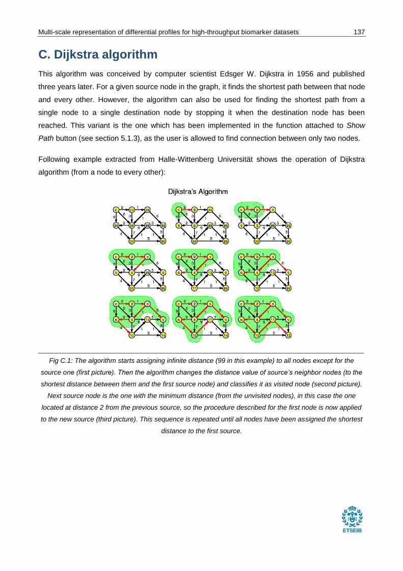
Multi-scale representation of differential profiles for high-throughput biomarker datasets 137
C. Dijkstra algorithm
This algorithm was conceived by computer scientist Edsger W. Dijkstra in 1956 and published
three years later. For a given source node in the graph, it finds the shortest path between that node
and every other. However, the algorithm can also be used for finding the shortest path from a
single node to a single destination node by stopping it when the destination node has been
reached. This variant is the one which has been implemented in the function attached to Show
Path button (see section 5.1.3), as the user is allowed to find connection between only two nodes.
Following example extracted from Halle-Wittenberg Universität shows the operation of Dijkstra
algorithm (from a node to every other):
____________________________________________________________________________________________________________
Fig C.1: The algorithm starts assigning infinite distance (99 in this example) to all nodes except for the
source one (first picture). Then the algorithm changes the distance value of source’s neighbor nodes (to the
shortest distance between them and the first source node) and classifies it as visited node (second picture).
Next source node is the one with the minimum distance (from the unvisited nodes), in this case the one
located at distance 2 from the previous source, so the procedure described for the first node is now applied
to the new source (third picture). This sequence is repeated until all nodes have been assigned the shortest
distance to the first source.


