Tellus (2009), 61A, 35–49 C© 2008 The AuthorsJournal compilation C© 2008 Blackwell Munksgaard

Printed in Singapore. All rights reserved

T E L L U S

Accessing extremes of mid-latitudinal wave activity:methodology and application

By R . V ITO LO 1∗, P. M . RU TI2, A . D ELL’AQ U ILA 2, M . FELIC I1,3, V. LU C A R IN I4

and A . SPER A N ZA 1, 1PASEF – Physics and Applied Statistics of Earth Fluids, Dipartimento di Matematica edInformatica, Universita di Camerino, Via Madonna delle Carceri – 62032 Camerino (MC), Italy; 2ENEA, via

Anguillarese 301 – 00060 S. Maria di Galeria, Roma, SP 091 Italy; 3Dipartimento di Matematica U. Dini, Universitadi Firenze, viale Morgagni 67/A – 50134 Firenze, Italy; 4Dipartimento di Fisica, Universita di Bologna, viale Berti

Pichat 6/2 – 40126 Bologna, Italy

(Manuscript received 30 September 2007; in final form 18 September 2008)

A B S T R A C TA statistical methodology is proposed and tested for the analysis of extreme values of atmospheric wave activity atmid-latitudes. The adopted methods are the classical block-maximum and peak over threshold, respectively based onthe generalized extreme value (GEV) distribution and the generalized Pareto distribution (GPD). Time-series of the‘Wave Activity Index’ (WAI) and the ‘Baroclinic Activity Index’ (BAI) are computed from simulations of the GeneralCirculation Model ECHAM4.6, which is run under perpetual January conditions. Both the GEV and the GPD analysesindicate that the extremes of WAI and BAI are Weibull distributed, this corresponds to distributions with an upper bound.However, a remarkably large variability is found in the tails of such distributions; distinct simulations carried out underthe same experimental setup provide sensibly different estimates of the 200-yr WAI return level. The consequencesof this phenomenon in applications of the methodology to climate change studies are discussed. The atmosphericconfigurations characteristic of the maxima and minima of WAI and BAI are also examined.

1. Introduction

Recently, different aspects of the general circulation of the at-mosphere have been investigated within the framework of eithervery simplified models or state-of-the-art GCMs, namely:

(1) the statistical properties, specifically extreme value statis-tics, of time-series of total energy generated by a baroclinicmodel of intermediate complexity for the atmospheric mid-latitudes (Felici et al., 2007a,b; Lucarini et al., 2007a,b);

(2) the description of wave propagation in the mid-latitudeatmosphere as simulated by a state-of-the-art coupled GCMs(simulations for the IPCC report) and associated products suchas reanalyses (Dell’Aquila et al., 2005; Ruti et al., 2006; Lucariniet al., 2007c).

While in the papers cited in (1) the procedures concerning ex-treme statistics and their parametric inference have been defined,

∗Corresponding author.Current address: School of Engineering, Computing and Mathematics,University of Exeter, Harrison building, North Park Road, Exeter, EX44QF, UK.e-mail: r.vitolo@exeter.ac.ukDOI: 10.1111/j.1600-0870.2008.00375.x

in the papers quoted in (2), dynamically oriented climate met-rics aimed at capturing the basic statistical properties of thefundamental features of the mid-latitude atmospheric variability– for example, synoptic baroclinic waves and planetary waves– have been introduced with the purpose of auditing GCMs andreanalyses. In this paper our purpose is to join the two researchstreams described above. Namely, we aim at developing a soundmethodology to attack the meteo-climatic problem of determin-ing the sensitivity of the (extreme) statistics of mid-latitudinaldisturbances to CO2 increase. The change in the statistics ofmid-latitude disturbances is considered a complex issue, as itis not obvious to determine which mechanisms are involved inthe change of the meridional temperature gradient at the variouspressure levels. The method of investigation we propose is basedon performing rigorous statistical analysis of extreme values of‘dynamically oriented metrics’.

The Northern Hemisphere mid-latitude variability is mainlydriven by large-scale (specifically: planetary scale) processeswhich affect, at different spatial and temporal scales, the variabil-ity of surface parameters (i.e. precipitation, wind, temperature).The latter parameters are those typically observed in the me-teorological networks and stored in the records. Nevertheless,time-series of sufficient length, suitable for reliable statisticalanalysis of extreme values, are not always available. This has

Tellus 61A (2009), 1 35

P U B L I S H E D B Y T H E I N T E R N A T I O N A L M E T E O R O L O G I C A L I N S T I T U T E I N S T O C K H O L M

SERIES ADYNAMIC METEOROLOGYAND OCEANOGRAPHY

36 R. VITOLO ET AL.

sometimes led the researchers to adopt weaker criteria for theselection of events to be used for analysis of extreme value statis-tics. In parametric inference this may introduce a substantial bias(Felici et al., 2007a); in practice, different studies based on thesame data may obtain different quantitative results.

With respect to observations, the usage of model-generateddata has the advantage that it makes it possible to satisfy thenecessary requirements of length and quality of the record, dis-cussed in, for example, Felici et al. (2007a). Indeed, statisti-cal analysis of extreme events has been successfully applied totime-series of surface parameters produced by climate models.Beniston et al. (2007) consider heat waves, heavy precipitation,drought, wind storms and storm surges changes between presentand future climate on the basis of regional climate model sim-ulations produced by the PRUDENCE project. Potential futurechanges in temperature and precipitation extremes have been ex-amined in an ensemble of global coupled climate models used forthe preparation of the Fourth IPCC Assessment Report (Kharinet al., 2007). Temperature and precipitation extremes were al-ready considered in Zwiers and Kharin (1998), Kharin andZwiers (2000). For evident reasons, most of the research onextremes in climate models focuses on surface parameters suchas temperature, precipitation and wind. Here, we wish to explorea different aspect: extremes of planetary and baroclinic atmo-spheric waves. Obviously, surface fields are strongly influencedby planetary-scale driving processes, but the characterization onsound theoretical grounds of a well-defined relation between thetwo is an open (and very hard) problem. One way of tackling thisis through statistical downscaling, see, for example, Friederichsand Hense (2007).

Among the dominant physical processes featured in the mid-latitude atmospheric dynamics, the synoptic waves and the in-teraction between ultra-long waves having zonal wavenumbersmaller than five (Bordi et al., 2004) and topography are mainingredients. The synoptic travelling perturbations can be repre-sented as high-frequency high-wavenumber eastward propagat-ing spectral features, characterized by periods of order 2–7 dand by spatial scales of a few thousand kilometres. These per-turbations can be associated with the release of available energydriven by conventional baroclinic conversion (Blackmon, 1976;Speranza, 1983; Wallace et al., 1988), so that they are oftenreferred to as baroclinic waves. On the other hand, so-calledplanetary waves, which interact with orography (Charney andDeVore, 1979; Charney and Straus, 1980; Buzzi et al., 1984;Benzi et al., 1986) and are catalysed by the subtropical jet(Benzi and Speranza, 1989; Ruti et al., 2006), play a dom-inant role in the low-frequency low-wavenumber spectral re-gion of so-called stationary waves, whose characteristic timeand space scales belong to the interval 10–45 d and 7000–15 000 km, respectively (Hansen and Sutera, 1986).

The methodology of the present work consists in analysing thestatistics of extreme values (in the parametric setting) for indexeslarge-scale atmospheric activity. A state-of-the-art GCM is run

in perpetual winter conditions for present-day atmospheric CO2

concentrations. We generate time-series of the Wave ActivityIndex (WAI) and of the Baroclinic Activity Index (BAI), whichmay be considered as proxies of the activity of the planetary andsynoptic waves, respectively (Benzi et al., 1986; Hansen andSutera, 1986; Dell’Aquila et al., 2007). Extreme value analysisis then performed by fitting generalized extreme value (GEV)distributions and generalized Pareto distributions (GPD) (Coles,2001; Felici et al., 2007a,b) on subsequences of ‘extreme values’extracted from the generated time-series. For the GEV, the ex-treme values are defined as maxima (or minima) computed overblocks of sufficiently large size, whereas for the GPD the ex-tremes are values exceeding a sufficiently high threshold (for thisreason, the latter is also called the peaks over threshold method– POT for shortness). The aim of studying the extremes of theWAI and BAI is to identify dynamically meaningful features ofthe general atmospheric circulation whose response under CO2

increase can be accurately assessed. The latter issue is subject ofcurrent research by some of the authors. We emphasize that theabove methods provide a common ground which can simplifythe comparison of results from different studies, compare with,for example, Beniston et al. (2007).

We now give an outline of the paper. A short description ofthe model, metrics and statistical methodology can be found inSection 2. The general statistical properties of the time-seriesare analysed in Section 3, whereas the extreme value analysis isreported in Section 4. Conclusions and lines of future researchare summarized in Section 6.

2. Data and methods

2.1. Description of the model and experimental setup

The atmospheric model used in this study is ECHAM4.6, anevolution of the model used by Roeckner and Arpe (1995),belonging to the fourth generation of GCM developed at theMax Planck Institute for Meteorology in Hamburg. It is an evo-lution of the spectral weather prediction model of the Euro-pean Centre for Medium Range Weather Forecasts (Simmonset al., 1989). ECHAM4 uses the spectral transform methodfor ‘dry dynamics’ while water vapour, cloud water and traceconstituents are advected by using a shape-preserving semi-Lagrangian scheme (Williamson and Rasch, 1994). The modelatmosphere is vertically resolved in 19 layers, from the surfaceup to 10 hPa. The model contains a set of parametrization forunresolved or not explicitly represented dynamical and physi-cal processes, including radiation (Fouquart and Bonnel, 1980;Morcrette, 1991), cumulus convection (Tiedke, 1989; Nordeng,1994) stratiform clouds (Roeckner, 1995), gravity wave drag(Miller et al., 1989), vertical diffusion and surface fluxes, landsurface processes and horizontal diffusion. A summary of the de-sign and performance of ECHAM4 can be found in Roeckner andArpe (1995).

Tellus 61A (2009), 1

EXTREMES OF MID-LATITUDINAL ACTIVITY 37

The simulations analysed in this paper have been performedat T30 spectral horizontal resolution, corresponding approxi-mately to a grid of 3.75◦ × 3.75◦. The GCM has been run for600 model months (30 d each), under perpetual January condi-tions, with present-day value of CO2 concentration (360 ppmv).The sea surface temperature (SST) and sea ice cover are keptconstant in time and fixed to the climatological mean of themonth of January. The choice of using simulations without sea-sonal cycle has a two-fold motivation, first of all, mid-latitudeatmospheric processes which might be affected by the climatechange, specifically the baroclinic activities, ‘take place underwinter conditions’ (Blackmon, 1976). Moreover, stationarity im-plies that there is no need to detrend the data; for inference ofextreme values this is an important advantage, since it allowsto reduce the number of parameters which are necessary in thestatistical model. This, in turn, allows to more clearly understandthe nature of variability in the time-series, see the discussion inFelici et al. (2007b).

2.2. Wave indexes used for the computationof time-series

Our study focuses on the Northern Hemisphere mid-latitudeatmospheric winter variability, therefore, we consider the lat-itudinal belt 30◦N–60◦N, where both the baroclinic and thelow-frequency planetary wave activities are present in theECHAM4.6 model. The 500 hPa geopotential height field islatitudinally averaged over this belt, to define a one-dimensionallongitudinal field representative of the atmospheric variability atmid-latitudes. We have verified that the results presented beloware not sensitive with respect to small variations in the latitudinalband, this is compatible with the fact that they mainly refer toplanetary-scale coherent atmospheric features. We choose the500 hPa geopotential height because it is one of the typical vari-ables used for the study of the planetary and synoptic scale at-mospheric circulation (Blackmon, 1976) and for the comparisonof different atmospheric data sets of climatological relevance.The indexes of dynamical activity for large-scale features of themid-latitude troposphere are computed according to the follow-ing procedure:

(1) the 500 hPa geopotential height field Z(λ, φ) is averagedwith respect to latitude φ over the latitudinal band boundedbetween 30◦N and 60◦N;

(2) for each day, the 500 hPa geopotential height is Fourierdecomposed in the longitudinal direction λ;

(3) an index is finally computed from the variance associatedto the Fourier coefficients Zk for k ranging from k1 up to kn:

Zk1,kn(t) =

(kn∑

k=k1

2|Zk(t)|2) 1

2

. (1)

The Wave Activity Index (Benzi et al., 1986; Hansen andSutera, 1986), or WAI, is then computed as the root mean square

of the zonal wavenumbers 2–4 of the winter 500 hPa geopotentialheight variance over the channel 30◦N–60◦N, that is, formula (1)with n = 3, k1 = 2 and k3 = 4. Furthermore, an index of synopticdisturbances has been computed using n = 3, k1 = 6 and k3 = 8;we refer to this as the BAI. The physical meaning of the aboveintroduced WAI and BAI is further discussed in Section 3.

2.3. Statistical inference of extreme values

We assume that the time-series generated by the ECHAM model(see Sections 2.1 and 2.2) are realizations of an unknownstochastic process and we use these time-series to perform twokinds of ‘parametric inferences’: point and interval estimations.Two parametric models are chosen for the statistical analysisof extremes: the GEV distribution and the GPD. Different in-ferential procedures are associated to the GEV and GPD: forthe former one typically adopts the ‘annual maximum’ method,whereas the latter is used in conjunction with the POT method(Coles, 2001; Smith, 2004). The GEV distribution function is

G(x) = exp

[−

(1 + ξ

x − μ

σ

)−1/ξ

+

], (2)

where the notation F(x)+ means the following: F(x)+ = F(x)for all x such that F(x) > 0 and F(x)+ = 0 otherwise. For ξ = 0,the GEV reduces to the Gumbel distribution (see Coles, 2001).Given a time-series, the distributional parameters (μ, σ , ξ ) areinferred by maximum likelihood procedures from sequences ofblock maxima extracted from the time-series.1 The methodol-ogy has been described in detail in Felici et al. (2007a,b), alsosee Coles (2001), Smith (2004) for basic theory and more ex-amples. It should be emphasized that the GEV model is validonly ‘asymptotically’. More precisely, one has to assume that theobserved time-series is the realization of a stationary stochasticprocess Xi belonging to the so-called maximum domain of at-traction (Resnick, 1987; Malevergne et al., 2006); denoting themaximum of the first n observations by M∗

n , one must assumethat there exist constants an and bn such that the normalizedmaximum Mn = (M∗

n − bn)/an converges to a non-degeneratedistribution G. Under these assumptions, G is of the form (2). Inthe applications, the parent process Xi is a priori unknown andit is, therefore, not possible to determine whether the constantsan and bn exist or not; one tacitly assumes that they do exist.At any rate, the constants an and bn can be ‘absorbed’ in thepoint estimates of the parameters μ and σ , assuming that oneis in the asymptotic range of the validity of the GEV, that is,

1 In environmental studies, a typical length for the blocks is 1 yr. Forexample, this overcomes the problem of seasonal trend in the data. Fromthis derives the name of ‘annual maximum’ method.

Tellus 61A (2009), 1

38 R. VITOLO ET AL.

Pr (Mn ≤ x) ≈ G(x), then

Pr(M∗n ≤ x) = Pr(Mn ≤ (x − bn)/an) =

= exp

{−

[1 + ξ

(x − μ∗

σ ∗

)]−1/ξ∗}, (3)

where μ∗ = anμ + bn, σ ∗ = anσ and ξ ∗ = ξ . This implies thatthe point estimates of GEV parameters μ∗ and σ ∗, as inferredby the block-maximum method, depend on the block length,whereas ξ ∗ is independent (asymptotically). Therefore, the as-sessment of the stability of the point estimates of ξ ∗ as blocklength is varied gives an indication of goodness-of-fit.

The distribution function of the GPD is

H (x) = 1 −(

1 + ξy

σ

)−1/ξ

+. (4)

Under rather general conditions, the GPD is the limit of thedistribution of a random variable X conditionally on exceedinga (high) threshold u. More precisely, by defining, for y > 0,

Fu(y) = P [X > u + y|X > u], (5)

then for large u the conditional distribution Fu tends to (4). Itturns out that the GEV and the GPD are very closely related;Pickands’ theorem (Pickands, 1975) states that for any sequenceX1, X2, . . . with a given common term X, a GPD arises fromthe large threshold limit of Fu in (5) if and only if there existnormalizing constants an, bn and a non-degenerate distributionfunction G such that

P [(Mn − bn)/an ≤ x] → G(x). (6)

In this case, writing G(x) as in (2), the shape parameter ξ isthe same as in the GPD (4), whereas the scale parameters arerelated by

σ = σ + ξ (u − μ). (7)

Given a sequence of independent and identically distributeddata x1, . . . , xn, extreme value modelling with the GPD isachieved by first selecting all exceedances over a sufficientlyhigh threshold u. Suppose that there are nexc ordered exceedancesx(1) ≥ x(2) ≥ . . . ≥ x(nexc) > u and denote the threshold excessesby yj = x(j ) − u for j = 1, . . . , nexc. Then, the yj are consideredas independent realizations of a random variable whose distri-bution can be approximated by a member of the GPD family.A suitable choice for the threshold u can be obtained by exam-ining the ‘mean excess’ plot (also known as mean residual lifeplot). This is based on the following idea: suppose that the ex-ceedances above a threshold u0 are ‘exactly’ GPD-distributed.Then the same holds for all thresholds u larger than u0 and, by(7), the mean of the excesses above threshold u is given by

E[X − u|X > u] = σu

1 − ξ= σu0 + ξ (u − u0)

1 − ξ. (8)

An empirical estimate for the mean excess is provided by thesample mean of the threshold excesses; by (8), the latter is ex-

pected to vary linearly with u, at least for sufficiently high valuesof u, for which the GPD approximation is valid. Therefore, suit-able threshold values are identified by looking for linearity inthe plot of points

(u,

1

nexc

nexc∑i=1

(x(i) − u)

), u ∈ [umin, umax]. (9)

Once a value for u has been selected, parameter estimation iscarried out by the maximum likelihood method, which also pro-vides confidence intervals. Model checking is performed by avariety of methods: among them, probability, quantile, densityand return level plots. Also, the stability of the estimated modelcan be assessed by examining several fits obtained by vary-ing the threshold. We refer to Coles (2001), Smith (2004) fordetails. A standard chi-squared test is used to assess goodness-of-fit (Perrin et al., 2006). The number of degrees of freedom ofthe chi-squared distribution is computed here as the number ofclasses minus four for the GEV (three for the GPD), to accountfor the parameters which are estimated from the data by themaximum likelihood. The number of classes may vary betweena maximum of 20 and a minimum of 9, to have at least fiveresidual degrees of freedom.

An important feature of the time-series analysed in the presentpaper is that they possess a non-negligible amount of autocorre-lation. In the GEV modelling framework, this typically does notcause serious problems; taking blocks of sufficiently large sizeyields uncorrelated sequences of block maxima. Therefore, onecan apply the GEV method as though the maxima were inde-pendent. However, this is not possible in the GPD approach: fortime-series with autocorrelation, threshold exceedances tend tooccur in ‘clusters’ and there is no general theory which specifiesthe joint distribution of neighbouring excesses (and, therefore,the likelihood function). A simple and widely used techniqueto counter this problem is the usage of so-called ‘decluster-ing’ and is based on the idea that clusters of exceedances areasymptotically independent (Hsing, 1987). ‘Runs declustering’(Leadbetter et al., 1989) consists in marking exceedances as be-longing to the same cluster if they are separated by fewer than afixed number r (the ‘run length’) of consecutive values below thethreshold. Once clusters are identified, the GPD is fitted to thecluster maxima. We emphasize that the selection of the declus-tering parameter r is largely arbitrary. A more sophisticateddeclustering scheme, based on the estimation of the extremalindex, is proposed by Ferro and Segers (2003). However, forsimplicity runs declustering is used in the present paper.

A convenient way to summarize the statistical properties ofextreme values is the ‘return level’. Given a number p with 0 <

p < 1, the return level associated with the ‘return period’ 1/p isdefined as the value zp that has a probability p to be exceededby the block maxima of the time-series. In the GEV modellingframework, a maximum likelihood estimator for zp is obtainedby plugging the estimates for (μ, σ , ξ ) into the formulae for the

Tellus 61A (2009), 1

EXTREMES OF MID-LATITUDINAL ACTIVITY 39

quantiles of G(x), obtained by inverting (2):

z∗p =

{μ∗ − σ∗

ξ∗ {1 − [− log(1 − p)]−ξ∗ } forξ ∗ = 0,

μ∗ − σ ∗ log[− log(1 − p)] forξ ∗ = 0.(10)

Confidence intervals for zp may be obtained from those of (μ∗,σ ∗, ξ ∗) by the ‘delta method’ (Coles, 2001; Felici et al., 2007a).Notice that the delta method makes explicit use of the formof the likelihood. When referring to the estimates of the GEVparameters or of the return levels, for simplicity we will omit thestar, taking for granted the notion that the inferred values maydepend on the selected block length.

Similarly, in the GPD modelling approach, the m-observationreturn level is defined as the level xm which is exceeded onaverage every m observations (in this case, p = 1/m). Again, theestimated values of (σ , ξ ) are plugged into the quantile formulafor the GPD, yielding the maximum likelihood estimator for xm:

xm = u + σ

ξ

[(mζu)ξ − 1

], ζu = nexc

n, (11)

where nexc is the number of exceedances and n is the total numberof observations. If declustering is applied, however, one needsto use the rate at which clusters occur, rather than the rate of allexceedances: this leads to the formula

xm = u + σ

ξ

[(mζuθ )ξ − 1

], ζu = nexc

n, θ = nclu

nexc, (12)

where θ is an estimate for the extremal index and nclu is thenumber of observed clusters (Coles, 2001). It is the latter formulathat we will use for computation of return levels in the GPDframework.

All computations in this paper have been carried out withthe statistical software R (R Development Core Team, 2008),available at www.r-project.org under the GPL license. Thelibraries ismev, which is an R-port of the routines written byStuart Coles as a complement to Coles (2001), and fExtremes

(both downloadable at www.cran.r-project.org) have beenused, as well as self-programmed routines.

3. Statistics of wave activity: a general overview

In this section, we first discuss the physical meaning of the WAIand BAI introduced in Section 2.2, by giving a brief historicalaccount. After this, the statistical properties of the time-seriesgenerated by the ECHAM model are discussed.

One of the classical problems in understanding the generalatmospheric circulation is to characterize the recurrent atmo-spheric patterns of flow which are observed at mid-latitudes inthe Northern Hemisphere winters (Rex, 1950; Baur, 1951; Dole,1983). The practical need motivating this research effort is two-fold: the feasibility of extended range weather forecasts and thedetection of climate change (Corti et al., 1999). As a matterof fact, it still is a subject of debate whether the large-scaleatmospheric circulation undergoes fluctuations around a sin-

gle equilibrium (Nitsche et al., 1994; Stephenson et al., 2004)or multiple equilibria (Charney and DeVore, 1979; Benzi andSperanza, 1989; Hansen and Sutera, 1995a; Mo and Ghil, 1988;Ruti et al., 2006). Hansen and Sutera (1986) find bimodality inthe statistical distribution of time-series of the WAI computedfrom observed data and orographic resonance theories providetheoretical support to the hypothesis of a multimodal distribu-tion for the activity of planetary waves. Specifically, Charneyand DeVore (1979) propose that the interaction between zonalflow and wavefield (via form-drag) explains the occurrence ofmultiple equilibria for the amplitude of planetary waves. How-ever, in their barotropic theory, the transitions between the twoquasi-stable equilibria involve variations of the mean westerlieswhich are much too large (�u ≈ 40 ms−1) with respect to ob-servations (Malguzzi and Speranza, 1981; Benzi et al., 1986).In Ruti et al. (2006), it has been shown that the bimodality ofstatistics of the planetary waves is modulated by the intensityof the subtropical jet, in accordance with the theoretical findingsof Benzi et al. (1986).

Taking into account these features of the general circulationof the atmosphere, the model simulations gathered by the IPCCpossess a reasonable skill in reproducing the high-frequencycomponent of the spectral decomposition, less so for the low-frequency part (Calmanti et al., 2007; Lucarini et al., 2007c).In fact, considering the planetary wave index (WAI), few mod-els reproduce bimodality as in the two reanalyses data sets (Rutiet al., 2006; Calmanti et al., 2007). This highlights a still existingproblem for the coupled simulations to reasonably reproduce thelow-frequency component of the atmospheric flow. In the caseof ECHAM, the AMIP-like experiments show a similar defi-ciency. The ECHAM4.6 model we are using in this work showsa unimodal probability density function of the planetary waveindex (WAI). The results of the IPCC simulation intercompari-son (Calmanti et al., 2007; Lucarini et al., 2007c) suggest thatthe low resolution adopted in the present setup is not the mainfactor affecting the lack of bimodality.

Figure 1a displays the empirical cumulative distribution func-tions of the WAI and BAI time-series generated by the ECHAMmodel in the present setup (see Section 2.1). The correspondingprobability density functions, shown in the panel b, are esti-mated using the kernel technique of Silverman (1986), wherethe smoothing parameter has been chosen as a Gaussian best-fit for each index. Regarding the first statistical moments ofthe time-series (see Table 1), we first note that both the meanvalue and the standard deviation of WAI are much larger thanthose of BAI. This confirms that a large portion of the planetary-scale activity is concentrated on the spatial scales pertainingto the planetary waves (Dell’Aquila et al., 2005; Lucarini et al.,2007c). Confidence intervals have been computed using a block-bootstrap method which takes care of the time autocorrelationof the time-series (Davison and Hinkley, 1997). Basically wehave that the variance of the mean varies as s/(L/τ ), where sis the sample variance, L is the length of the time-series and

Tellus 61A (2009), 1

40 R. VITOLO ET AL.

0 50 100 150

0.0

0.2

0.4

0.6

0.8

1.0empirical cumul. distr. f.

WAI,BAI(m)

ecdf

waibai

(a)

0 50 100 150

0.00

0.01

0.02

0.03

0.04

density

WAI,BAI(m)

pdf

waibai

(b)

Fig. 1. Empirical cumulative distribution function (a) and probabilitydensity function (b) of the time-series of the WAI (thin lines) and BAI(thick lines) indexes. The PDF has been estimated using the kerneltechnique of Silverman (1986).

Table 1. 95% confidence interval of the mean and standard deviation(both expressed in m) of the WAI and BAI time-series

Mean (95% confidence interval) SD

WAI, 1CO2 93.0 ± 0.9 21.0BAI, 1CO2 35.0 ± 0.3 9.0

τ is its decorrelation time (the latter is estimated by requir-ing that the linear autocorrelations drop below 1/e). We havethat in both cases τ ≈ 6 for the BAI and τ ≈ 12 for the WAItime-series.

Our interest in characterizing the extreme value statistics ofthe WAI and BAI falls in the context mentioned above; specifi-cally we aim at understanding which properties may be relevantto assess climate change and the physical processes involved init at the level of general atmospheric circulation. We empha-size that the bimodality (or lack thereof) of the time-series doesnot affect the applicability of the GEV/GPD methods: extremevalue analysis aims at characterizing the upper or lower tailsof a stochastic process, whereas bimodality takes place in thecentral part of the probability distribution function. More specif-ically, one can design a stochastic process having a pre-specifiedtail behaviour, with any other kind of behaviour (unimodal, bi-modal, multimodal, discontinuous) in the central part, so the twoare unrelated.

4. Extreme value analysis

In this section, the block-maximum and threshold-exceedancemethods described in Section 2.3 are applied to the time-seriesof WAI and BAI indicators generated from the ECHAM model.

4.1. GEV analysis

In the block-maximum approach, the time-series are subdividedinto B data blocks, each containing D daily values, where B =L/D and L is the total length (number of daily observations)of the time-series. Maximum values over each data block arecomputed, producing the sequences of values from which theGEV parameters (μ, σ , ξ ) are estimated. The same procedure isapplied to sequences of block minima of the time-series. Sincethe GEV is a limit distribution, obtained in the limit of L and Dgoing to infinity (see Section 2.3), to avoid bias in the estimates itis not sufficient to take a block length, that is, slightly larger thanthe decorrelation time scale τ (see Section 3). This implies thatD = 100 d is likely to be the minimum acceptable block length.To assess the sensitivity and stability of the estimates, we havetried a few values for D: all of them are such that L is exactlydivisible by D, to avoid bias due to a different length of the lastdata block. In Fig. 2, we display the estimated values of ξ (withthe related uncertainty) against the value of D used for inference.The estimates of ξ are rather stable after sampling uncertaintyis taken into account. Of course, uncertainties increase with D,

50 100 150 200 250 300 350

0.0

0.1wai, max

block length

xi

(a)

50 100 150 200 250 300 350

0.0

0.1bai, max

block length

xi

(b)

Fig. 2. Estimated values of the shape parameter ξ as a function of theblock length D over which maxima are computed, for the WAI (a) andBAI (b) time-series. 95% confidence intervals (average plus and minustwo standard deviations) are added.

Tellus 61A (2009), 1

EXTREMES OF MID-LATITUDINAL ACTIVITY 41

Probability Plot

Empirical

Mod

el

0.0 0.5 1.0

0.0

0.5

1.0Quantile Plot

Model

Em

piric

al

89 130 171

89

130

171

100

120

140

160

Ret. Period (# blocks)

Ret

urn

Leve

l (m

)

Return Level Plot Density Plot

WAI (m)

pdf

100 140 180

0.00

0.01

0.02

0.03

(a)

Probability Plot

Empirical

Mod

el

0.0 0.5 1.0

0.0

0.5

1.0Quantile Plot

Model

Em

piric

al

109 140 171

109

140

171

110

120

130

140

150

160

170

Ret. Period (# blocks)

Ret

urn

Leve

l (m

)

Return Level Plot Density Plot

WAI (m)

pdf

110 130 150 170

0.00

0.01

0.02

0.03

(b)

Probability Plot

Empirical

Mod

el

0.0 0.5 1.0

0.0

0.5

1.0Quantile Plot

Model

Em

piric

al

129 150 171

129

150

171

130

140

150

160

170

Ret. Period (# blocks)

Ret

urn

Leve

l (m

)

Return Level Plot Density Plot

WAI (m)

pdf

130 150 170

0.00

0.01

0.02

0.03

(d)

Probability Plot

Empirical

Mod

el

0.0 0.5 1.0

0.0

0.5

1.0Quantile Plot

Model

Em

piric

al

119 145 171

119

145

171

120

130

140

150

160

170

Ret. Period (# blocks)

Ret

urn

Leve

l (m

)

Return Level Plot Density Plot

WAI (m)

pdf

120 140 160

0.00

0.01

0.02

0.03

(c)

Fig. 3. Diagnostic plots for the GEV fits of the WAI computed with sequences of maxima with block length D = 50 (a), 100 (b) 200 (c) and 300 (d).

since one is using less values for the inference. Accordingly, wechoose D in such a way that the inferences are reasonably stableand that the associated uncertainties are not too large. There is agood deal of subjectivity in this choice: as usual in GEV-basedanalysis, one has to adopt a reasonable compromise betweenlong and short data blocks, which boils down to a trade-offbetween variance and bias (Coles, 2001; Felici et al., 2007a,b).

For the time-series of WAI and BAI, block lengths of D = 100or D = 200 seem reasonable: they are large enough to ensuredecorrelation of the extreme values and the point estimates ofthe GEV parameters remain almost constant for D ≥ 100. Thediagnostic plots in Fig. 3 confirm that there is nothing wrong withthe inferences obtained for D = 100, 200, 300: for example, thedisplacements of points from the diagonals are relatively smallin the probability and quantile plots. More graphical diagnostics(not shown), analogous to those in Figs. 2 and 3, suggest that the

same conclusions also hold for the minima. The choice D = 50is not appropriate for various reasons: first of all, a non-trivialamount of linear autocorrelation persists in the relative sequenceof block maxima (figure not shown). Second, the quantile plotreveals lack-of-fit at both ends of the empirical distribution andthe confidence intervals of the return level plot look too narrow,indicating that the balance leans towards bias in the bias-versus-variance trade-off discussed above.

Plots of the return levels zp as functions of the return period(expressed in days) are given in Fig. 4 for the maxima and inFig. 5 for the minima, for D = 100 and 300. For the minima,estimation is performed by first multiplying the time-series by−1, then performing the inference on the maxima, then mul-tiplying again by −1. We observe a very good agreement ofthe return levels for sufficiently large return periods: this con-firms the stability of the inferences with respect to block length.

Tellus 61A (2009), 1

42 R. VITOLO ET AL.

110

120

130

140

150

160

170

180

Return Period (years)

Ret

urn

Leve

l (m

)

0.5 1 5 10 50 200

wai,max

D=100D=300

(a)

wai,max

D=100D=300

(a)

50

55

60

65

70

75

80

85

Return Period (years)

Ret

urn

Leve

l (m

)

0.5 1 5 10 50 200

bai,max

D=100D=300

(b)

bai,max

D=100D=300

(b)

Fig. 4. Return level plots for maxima of the WAI (a) and BAI (b)time-series, using blocks of length D = 100 d (solid lines) and D = 300(dashed lines). Time is expressed in years (365 model days) andWAI/BAI in metres.

10

20

30

40

50

60

70

Return Period (years)

Ret

urn

Leve

l (m

)

0.5 1 5 10 50 200

wai,min

D=100D=300

(a)

wai,min

D=100D=300

(a)

10

15

20

25

Return Period (years)

Ret

urn

Leve

l (m

)

0.5 1 5 10 50 200

bai,min

D=100D=300

(b)

bai,min

D=100D=300

(b)

Fig. 5. Same as Fig. 4 for the minima of the same time-series.

However, the estimated uncertainties are in general fairly large:from a ‘physical’ point of view, a word of caution must be spenthere, because a small (in relative terms) variation of absolutevalue of WAI corresponds to a large variation in the correspond-ing planetary-scale fields. For example, the upper and lowerbounds of the 95% confidence interval for the 200-yr return

level of the WAI maxima differ by roughly 15.5 m. The WAIdifference between amplified wave patterns and zonal flow ofabout 20 m corresponds to local anomalies up to 200–300 m(Hansen and Sutera, 1995b).

4.2. GPD analysis

We now compare the results of the GEV analysis reported inthe previous section to those obtained by the GPD approach.Throughout this section, a run-declustering scheme is applied tothe data, with r = 10; we have verified that for larger values ofr (say, up to r = 20), the number of identified clusters does notchange much, whereas there are larger differences between thecases r = 0 and r = 1, 2.

The first step is to identify a suitable threshold u for theselection of exceedances. Mean excess plots for the WAI andBAI series are given in Fig. 6 (Fig. 7) for exceedances beyondhigh (below low) levels. This suggests the following intervalsof linearity: [135, 143] and [60, 65] for high levels of WAI andBAI, respectively; [35, 60] and [15, 20] for low levels of WAI andBAI, respectively. For each case, the GPD is fitted to the clustermaxima of the exceedances for a range of thresholds within theabove ranges. The resulting estimates of ξ , displayed below therespective mean excess plots, are consistent across the selectedrange. We have also plotted the estimates obtained with runlengths r = 3 and r = 20 (dashed and dotted lines, respectively).This shows that there is little sensitivity with respect to runlength, particularly so for larger thresholds.

We fix thresholds u of 136 and 60 for high levels of WAIand BAI, respectively. Return level curves computed by (12) areshown in Fig. 8 and reveal an excellent agreement with the GEVestimates obtained for D = 200, also see Tables 2 and 3. Thethresholds have been chosen within the ranges discussed above,in such a way that the number of identified clusters is not toodifferent from the number of block maxima used for the GEVinference. For u = 140, wider confidence intervals are obtainedfor WAI (shown with dotted lines in Fig. 8a), but the chi-squaredtest with 20 classes rejects the fit at the 95% level of confidence(the test with 19 classes is passed, with a t-value of 0.07 Table 2).All other tests do not indicate lack-of-fit and using a thresholdof 131 yield a plot (not shown) which is very similar to that foru = 136.

We also emphasize that the estimated value of the parameterξ is always negative, corresponding to a Weibull distribution(Coles, 2001), except for a few cases (not shown) where thenumber of values used for inference is too low and the samplinguncertainty is extremely large (indicating lack-of-fit). The sup-port of Weibull probability density functions is bounded fromabove, there exists a value z∞ = μ − σ/ξ which may be consid-ered as a return level with unbounded return period, since valueslarger than z∞ form a set having zero probability (the Weibullprobability density function is identically zero for those values).The fact that ξ is negative with overwhelming confidence is

Tellus 61A (2009), 1

EXTREMES OF MID-LATITUDINAL ACTIVITY 43

80 100 120 140 160

0

10

20

30

40

50

60wai

threshold (m)

Mea

n E

xces

s (m

)

(a)

30 40 50 60 70

0

10

20

30

40

bai

threshold (m)

Mea

n E

xces

s (m

)

(b)

55 60 65

0.0

0.2

Threshold (m)

Sha

pe

(d)

130 135 140 145

0.00.20.4

Threshold (m)

Sha

pe

(c)

Fig. 6. (a and b) Mean excess plots for high level exceedances of theWAI (a) and BAI (b) time-series. (c and d) Shape parameter ξ of theGPD distribution for the WAI (c) and BAI (d) time-series, estimatedfrom maxima of cluster exceedances for a range of values of thethreshold u. A run-declustering algorithm is used with r = 10 (solid lineand confidence bars), r = 3 (dashed lines) and r = 20 (dotted lines).

compatible with the existence of upper and lower bounds forthe considered indexes. In a much simpler model (Felici et al.,2007a), it has been shown that such bounds do exist, providing‘physical constraints’ of the system. For the ECHAM model,we interpret this result as follows: in a system with a finite en-ergy input, energy of the perturbations cannot grow indefinitely.Therefore, the probability density function of the (extreme) per-turbations is bounded and the shape parameter is negative. Thistheory is fully compatible with all of the estimates which we haveobtained from the simulation data. For more common physical

0

5

10

15

20

25

bai

threshold (m)

Mea

n E

xces

s (m

)

(b)

0.0

Threshold (m)

Sha

pe

(d)

0

10

20

30

40

50

60

wai

threshold (m)

Mea

n E

xces

s (m

)

(a)

0.00.2

Threshold (m)

Sha

pe

(c)

Fig. 7. Same as Fig. 6 for the exceedances below low levels.

variables, wind speeds in both extratropical latitudes (Perrinet al., 2006) and in tropical storms and hurricanes (Neumann,1987; Elsner et al., 2008) are often observed to be Weibull dis-tributed, whereas hydrological variables such as precipitationoften display heavy tails (with a positive value of the shape pa-rameter), see Coles (2001), Felici et al. (2007a), Smith (2004)for more references.

4.3. On the possibility of slow convergence of GEVestimators

In this section, we analyse the sensitivity of the extremevalue statistical properties with respect to changes in model

Tellus 61A (2009), 1

44 R. VITOLO ET AL.

140

150

160

170

180

190

Return Period (years)

Ret

urn

Leve

l (m

)

0.5 5 50 200 1000

wai,max

GEVGPD,u=136GPD,u=140

(a)

60

65

70

75

80

85

Return Period (years)

Ret

urn

Leve

l (m

)

0.5 5 50 200 1000

bai,max

GEVGPD,u=60GPD,u=63

(b)

Fig. 8. Joint GEV–GPD return level plots for the maxima-high levelexceedances of WAI (a) and BAI (b). The GEV maximum likelihoodestimates and 95% confidence intervals are plotted with dashed lines,whereas solid and dotted lines are used for GPD fits obtained with twodifferent threshold values. Empirical estimates (points) are added forthe GPD fit lower threshold. The estimated parameter values and otherinformation concerning the inferences are reported in Table 2 for WAIand in Table 3 for BAI.

configuration. Two runs of the ECHAM model, with CO2 con-centration equal to five times the present-day value (1800 ppmv)are carried out. For simplicity, the SSTs are kept the same asin the 1CO2 run examined in the rest of this paper. We empha-size that this rules out any interpretation of the results of thepresent section in terms of climatic change, based on the com-parison with the 1CO2 run. For this reason, such a comparisonis not even attempted. The present experiments aim exclusivelyat getting more information on the sensitivity of the statisticalestimates based on data generated by the ECHAM model, toestablish the experimental requirements for studies of climaticchange based on the present methodology.

The two 5CO2 runs only differ from each other in the initialcondition, the remaining parameters and settings being identicalto those described in Section 2.1. For this reason, time-seriesextracted from the two runs should be considered as differ-ent realizations of the same stochastic process and should pos-

Table 2. Summary of the GEV (top row) and GPD (bottom row) fitscorresponding to the inference in Fig. 8a (the GPD fits with r = 3 andthat with u = 131 are not shown in the plot). Standard errors for theparameters are reported inside parentheses, whereas nd is the numberof degrees of freedom for the chi-squared goodness-of-fit test

μ σ ξ B D t-value, nd

136.7 (1.1) 9.8 (0.8) −0.20 (0.06) 90 200 0.75 (15)

u σ ξ nclu r136 8.3 (1.0) −0.14 (0.07) 121 3 0.15 (16)136 9.0 (1.1) −0.16 (0.08) 105 10 0.18 (16)140 7.7 (1.3) −0.12 (0.11) 68 10 0.1 (15)131 9.1 (0.9) −0.13 (0.07) 187 10 0.39 (16)

Table 3. Same as Table 2 for the inference Fig. 8b. The GPD fit with r

= 3 is not shown in the plot

μ σ ξ B D t-value (nd)60.1 (0.5) 4.8 (0.4) −0.19 (0.07) 90 200 0.33 (15)

u σ ξ nclu r60 5.1 (0.8) −0.22 (0.11) 82 3 0.84 (16)60 5.1 (0.8) −0.21 (0.11) 81 10 0.85 (16)63 5.3 (1.1) −0.33 (0.16) 41 10 0.47 (16)

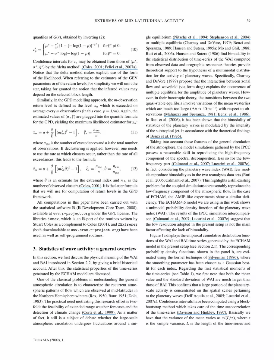
sess the same statistical properties. GEV analysis is carried outon time-series of WAI and BAI for these 5CO2 runs (to dis-tinguish them we refer to the second one as 5CO2Bis). For themaxima of the WAI, one obtains huge differences in the pointestimates of the return levels and even much larger variationsif confidence intervals are taken into account, see Fig. 9a. Thepoint estimates of the 1000-yr return levels of the WAI differ byroughly 15 m (an idea of the physically relevance of such a valueis given in a remark at the end of Section 4.1). A similar discrep-ancy is also found using the GPD method, although a smalleruncertainty is obtained (Fig. 9b). This suggests the followingscenario: even under identical experimental setup, except for theinitial condition from which the model is started, one may ob-tain quantitatively different point estimates for the return values.Now in the experimental setting which we have considered, thewide confidence interval helps us reject the hypothesis that thetwo populations are different. However, if shorter data blocksare used, then narrower confidence intervals might be obtained.In this case, the different experiments would obtain differentresults at the same level of confidence.

These discrepancies are largely accounted for by a few excep-tionally large values of the WAI in the 5CO2Bis series: for exam-ple, by taking away the two largest block maxima of 5CO2Bis,the difference in the return level plots is much smaller (Fig. 9c).Moreover, the remaining block maxima of 5CO2Bis are smallerthen the maximum of 5CO2. Similar considerations hold for theGPD method, see Fig. 9d. This suggests that there exist states of

Tellus 61A (2009), 1

EXTREMES OF MID-LATITUDINAL ACTIVITY 45

140

150

160

170

180

190

200Return Level Plot

Return period (years)

Ret

urn

leve

l (m

)

0.5 5 10 50 200 1000

(b)

140

150

160

170

180

190

200

Return Period (years)

Ret

urn

Leve

l (m

)

0.5 5 10 50 200 1000

Return Level PlotReturn Level Plot(a)

140

150

160

170

180

190

200

Return Period (years)

Ret

urn

Leve

l (m

)

0.5 5 10 50 200 1000

Return Level PlotReturn Level Plot(c)

140

150

160

170

180

190

200Return Level Plot

Return period (years)

Ret

urn

leve

l (m

)

0.5 5 10 50 200 1000

(d)

Fig. 9. (a) Return level plot obtained by the GEV method from the maxima of two distinct 5CO2 runs of the ECHAM model, see text for the details.(c) Same as (a), where the two largest block maxima of the 5CO2Bis series have been removed. (b and d) Same as (a and c), respectively, for a GPDfit of the same time-series; threshold values for (b and d) are equal to those used for Figs. 8 (a) and (b), respectively.

remarkable WAI amplitude which are visited very rarely by theECHAM model; it appears that to include such states in the anal-ysis, time-series of great length are necessary. This requirementis likely to be even more stringent when simulations by fullycoupled AOGCMs with seasonal cycle are examined. This phe-nomenon might bear relation to the slowness of convergence ofthe GEV estimators which has been found in a quasi-geostrophicmodel (Vannitsem, 2007) but also in a stochastic volatility pro-cess with long-memory modelling stock returns (Malevergneet al., 2006). We believe that assessing the speed of convergenceof the extreme value distribution estimators and its possible re-lation to long-memory processes (Maraun et al., 2004; Eichneret al., 2006) is of remarkable scientific and, in view of the en-visaged applications, societal importance.

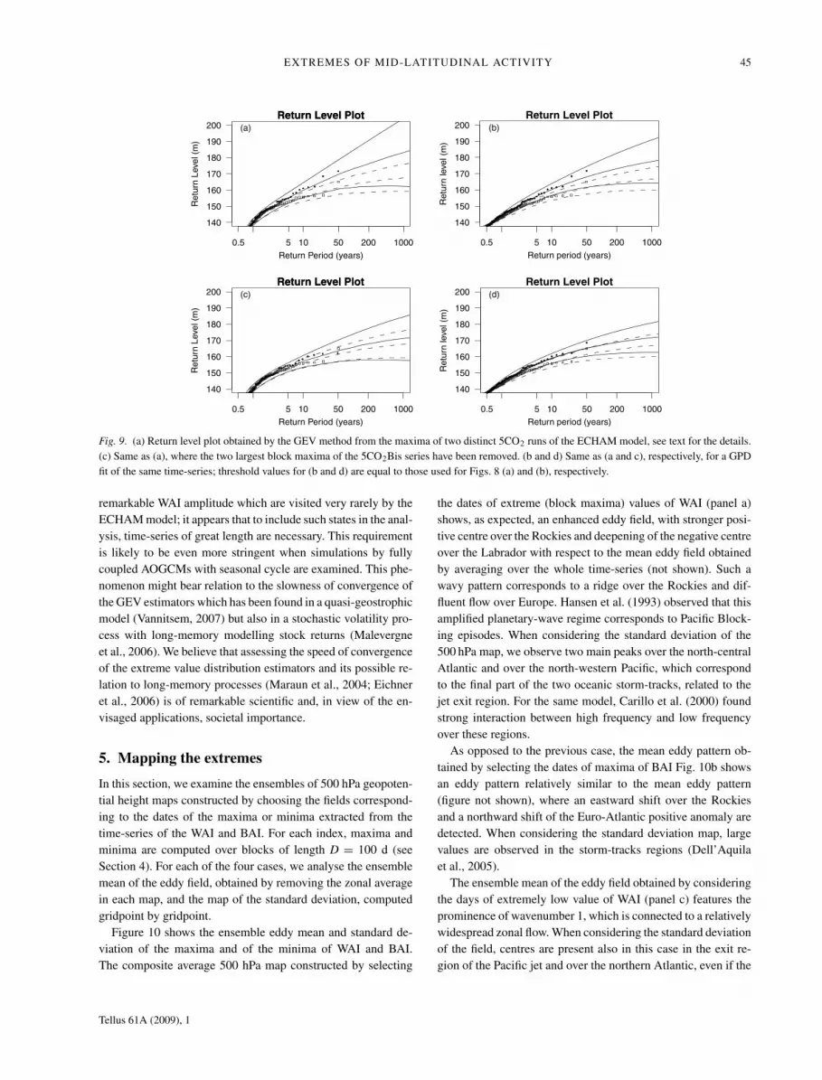
5. Mapping the extremes

In this section, we examine the ensembles of 500 hPa geopoten-tial height maps constructed by choosing the fields correspond-ing to the dates of the maxima or minima extracted from thetime-series of the WAI and BAI. For each index, maxima andminima are computed over blocks of length D = 100 d (seeSection 4). For each of the four cases, we analyse the ensemblemean of the eddy field, obtained by removing the zonal averagein each map, and the map of the standard deviation, computedgridpoint by gridpoint.

Figure 10 shows the ensemble eddy mean and standard de-viation of the maxima and of the minima of WAI and BAI.The composite average 500 hPa map constructed by selecting

the dates of extreme (block maxima) values of WAI (panel a)shows, as expected, an enhanced eddy field, with stronger posi-tive centre over the Rockies and deepening of the negative centreover the Labrador with respect to the mean eddy field obtainedby averaging over the whole time-series (not shown). Such awavy pattern corresponds to a ridge over the Rockies and dif-fluent flow over Europe. Hansen et al. (1993) observed that thisamplified planetary-wave regime corresponds to Pacific Block-ing episodes. When considering the standard deviation of the500 hPa map, we observe two main peaks over the north-centralAtlantic and over the north-western Pacific, which correspondto the final part of the two oceanic storm-tracks, related to thejet exit region. For the same model, Carillo et al. (2000) foundstrong interaction between high frequency and low frequencyover these regions.

As opposed to the previous case, the mean eddy pattern ob-tained by selecting the dates of maxima of BAI Fig. 10b showsan eddy pattern relatively similar to the mean eddy pattern(figure not shown), where an eastward shift over the Rockiesand a northward shift of the Euro-Atlantic positive anomaly aredetected. When considering the standard deviation map, largevalues are observed in the storm-tracks regions (Dell’Aquilaet al., 2005).

The ensemble mean of the eddy field obtained by consideringthe days of extremely low value of WAI (panel c) features theprominence of wavenumber 1, which is connected to a relativelywidespread zonal flow. When considering the standard deviationof the field, centres are present also in this case in the exit re-gion of the Pacific jet and over the northern Atlantic, even if the

Tellus 61A (2009), 1

46 R. VITOLO ET AL.

(a)

(m)

(b)

(m)

(c)

(m)

(d)

(m)

Fig. 10. The eddy ensemble mean (contour) and the standard deviation (shaded) of the 100-d maxima of WAI (a) and BAI (b) and of the 100-dminima of WAI (c) and BAI (d).

variability is much lower than what depicted in Fig. 10. As forthe maxima, the ensemble mean of the eddy field obtained byselecting the extremely low BAI events Fig. 10d is similar tothe mean eddy pattern (figure not shown), while the two stan-dard deviation maps feature larger variance in correspondencewith the Pacific and Atlantic jet exit regions, but with reducedvariability with respect to what shown in Fig. 10.

6. Summary and conclusions

In this paper, we have proposed a methodology for the analysis ofextreme atmospheric wave activity at mid-latitudes. The method-ology has been applied to various simulations obtained by theGeneral Circulation Model ECHAM4.6. The wave indexes wehave examined can be considered as proxies of planetary-scaleactivity at different spatial and temporal scales. The mid-latitudedynamics features upper planetary and synoptic waves as typ-ical ingredients. Since synoptic and planetary waves provide arelevant contribution to the meridional transport of energy andmomentum in the mid-latitudes, the physical processes drivingsuch phenomena are sensible ingredients for the characterizationof the climate system (Speranza, 1983). The statistical behaviourof extreme values of the various time-series is studied by theblock-maximum method (fitting GEV distributions) and by the

POT method (fitting GPDs). The statistical significance of theseresults has been thoroughly assessed by a variety of diagnostictools. The analysis of extreme values is complemented by anexamination of composite maps of the extremes of the maxima,to highlight the spatial patterns.

Rather large uncertainties are obtained here, both for the GEVparameters and for the return levels. It might be questionedwhether there are problems of convergence for the GEV estima-tor. In this sense, our results bear some resemblance with thoseby Vannitsem (2007), who finds that extremely long time-seriesare necessary to reach satisfactory convergence of the statisticalestimators in a quasi-geostrophic model. The fact that such alarge amount of uncertainty is obtained for the extreme valuestatistics even in the present, idealized simulations (no seasonalcycle) suggests the possibility that time-series of almost pro-hibitive length might be necessary for accurate estimations in amore realistic setup, such as an atmospheric GCM coupled witha slab ocean or even a fully coupled AOGCM with seasonalcycle. Of course, this problem is likely to be even more seriouswhen dealing with observed data or reanalyses, as sensitivitystudies with respect to length of the time-series cannot be car-ried out. As expected, usage of the GPD-based approach mayyield a somewhat reduced uncertainty. However, in our studyof two stationary runs which only differ in the intial condition

Tellus 61A (2009), 1

EXTREMES OF MID-LATITUDINAL ACTIVITY 47

(and, therefore, may be considered as two realizations of thesame stochastic process), a marked difference in the two pointestimates is obtained.

The analysis of the composite maps allow us to feature thespatial patterns associated with the extremes in low and highwavy regimes. The maxima in the WAI shows enhanced eddyfield, with stronger positive centre over the Rockies and deepen-ing of the negative centre over the Labrador. The correspondingstandard deviation features high amplitudes, where strong inter-action between high frequency and low frequency is observed.Considering the maxima of the BAI index, the standard devia-tion pattern is quite similar to what observed for the WAI, butstronger on the American east coast where the Atlantic storm-tracks origin. The eddy pattern is not enhanced as in the WAImaxima: this could suggest that the link between planetary andbaroclinic waves is not linear. The analysis of the relationshipbetween high and low frequencies will be further developed in astudy with AMIP-like simulations forced by SST from a globalscenario coupled simulation.

We conclude by remarking that, for the general strategy ofsetting up model comparisons, the statistical nature of the se-lected diagnostic indicators might be of essential importance.We believe that the indicators of planetary-scale activity consid-ered in the present paper and, particularly, the extreme statisticsof such indicators, can be used for model intercomparison asa complement to the surface parameters (such as temperature,precipitation, wind) typically examined in research on extremesin climate models.

7. Acknowledgments

This work has been partially funded by the CIRCE EU project(IP-036961) and by the MUR PRIN 2006 grant ‘Deterministicand statistical properties of large-scale vortices in the atmosphereand the ocean: a phenomenological, mathematical, numericalstudy’.

References

Baur, F. 1951. Extended range weather forecasting. In: Compendium of

Meteorology. Amer. Meteor. Soc., Boston, Massachussets, 814–833.Beniston, M., Stephenson, D. B., Christensen, O. B., Ferro, C. A. T.,

Frei, C. and co-authors. 2007. Future extreme events in Europeanclimate: an exploration of regional climate model projections. Clim.Change 81(Suppl. 1), 71–95.

Benzi, R. and Speranza, A. 1989. Statistical properties of low frequencyvariability in the Northern Hemisphere. J. Clim. 2, 367–379.

Benzi, R., Malguzzi, P., Speranza, A. and Sutera, A. 1986. The statisticalproperties of general atmospheric circulation. Observational evidenceand a minimal theory of bimodality. Quart. J. Roy. Meteorol. Soc. 112,661–674.

Blackmon, M. L. 1976. A climatological spectral study of the 500 mbgeopotential height of the Northern Hemisphere. J. Atmos. Sci. 33,1607–1623.

Bordi, I., Dell’Aquila, A., Speranza, A. and Sutera, A. 2004. On the mid-latitude tropopause height and the orographic-baroclinic adjustmenttheory. Tellus 56A, 278–286, doi:10.1111/j.1600-0870.2004.00065.x.

Buzzi, A., Trevisan, A. and Speranza, A. 1984. Instabilities of a baro-clinic flow related to topographic forcing. J. Atmos. Sci. 41, 637–650.

Calmanti, S., Dell’Aquila, A., Lucarini, V., Ruti, P. M. and Speranza, A.2007. Statistical properties of mid-latitude atmospheric variability. In:Nonlinear Dynamics in Geosciences (eds. A. Tsonis and J. Elsner).Springer, (New York, USA), ISBN 978-0-387-34917-6.

Carillo, A., Ruti, P. M. and Navarra, A. 2000. Storm tracks and meanflow variability: a comparison between observed and simulated data.Clim. Dyn. 16, 218–229.

Charney, J. G. and DeVore, J. G. 1979. Multiple flow equilibria in theatmosphere and blocking. J. Atmos. Sci. 36, 1205–1216.

Charney, J. G. and Straus, D. M. 1980. Form-drag instability, multipleequilibria and propagating planetary waves in baroclinic, orographi-cally forced, planetary wave systems. J. Atmos. Sci. 37, 1157–1176.

Coles, S. 2001. An Introduction to Statistical Modelling of Extremes

Values. Springer-Verlag, Berlin and Heidelberg, 208 pp.Corti, S., Molteni, F. and Palmer, T. N. 1999. Signature of recent climate

change in frequencies of natural atmospheric circulation regimes.Nature 398, 799–802.

Davison, A. C. and Hinkley, D. V. 1997. Bootstrap Methods and TheirApplication. Cambridge University Press, Cambridge.

Dell’Aquila, A., Lucarini, V., Ruti, P. M. and Calmanti, S. 2005. Hayashispectra of the Northern Hemisphere mid-latitude atmospheric vari-ability in the NCEP-NCAR and ECMWF reanalyses. Clim. Dyn., 25,639–652.

Dell’Aquila, A., Ruti, P. M. and Sutera, A. 2007. Effects of the baroclinicadjustment on the tropopause in the NCEP-NCAR reanalysis. Clim.Dyn. 28, doi:10.1007/s00382-006-0199-4.

Dole, R. M. 1983. Persistent anomalies of the extratropical NorthernHemisphere wintertime circulation. In: Large-Scale Dynamical Pro-

cesses in the Atmosphere, (eds. B. J. Hoskins and R. P. Pearce).Elsevier, New York, 95–109.

Eichner, J. F., Kantelhardt, J. W., Bunde, A. and Havlin, S. 2006. Extremevalue statistics in records with long-term persistence. Phys. Rev. E 73,016130.

Elsner, J. B., Jagger, T. H. and Liu, K. b. 2008. Comparison of Hurricanereturn levels using historical and geological records. J. Appl. Meteorol.Climatol. 47, 368–374.

Felici, M., Lucarini, V., Speranza, A. and Vitolo, R. 2007a. Extremevalue statistics of the total energy in an intermediate complexity modelof the mid-latitude atmospheric jet. Part I: stationary case. J. Atmos.

Sci. 64, 2137–2158.Felici, M., Lucarini, V., Speranza, A. and Vitolo, R. 2007b. Extreme

value statistics of the total energy in an intermediate complexitymodel of the mid-latitude atmospheric jet. Part II: trend detectionand assessment. J. Atmos. Sci. 64, 2159–2175.

Ferro, C. A. T. and Segers, J. 2003. Inference for clusters of extremevalues. J. R. Stat. Soc. 65B, 545–556.

Fouquart, Y. and Bonnel, B. 1980. Computations of solar heating of theEarth’s atmosphere. A new parametrization. Contrib. Phys. Atmos.

53, 35–62.Friederichs, P. and Hense, A. 2007. Statistical downscaling of extreme

precipitation events using censored quantile regression. Mon. Wea.

Rev. 135, 2365–2378.

Tellus 61A (2009), 1

48 R. VITOLO ET AL.

Hansen, A. R. and Sutera, A. 1986. On the probability density distri-bution of planetary-scale atmospheric wave amplitude. J. Atmos. Sci.43, 3250–3265.

Hansen, A. R. and Sutera, A. 1995a. The probability density distributionof planetary-scale atmospheric wave amplitude revisited. J. Atmos.Sci. 52, 2463–2472.

Hansen, A. R. and Sutera, A. 1995b. Large amplitude flow anoma-lies in Northern Hemisphere mid-latitudes. J. Atmos. Sci. 52, 2133–2151.

Hansen, A., Pandolfo, J. and Sutera, A. 1993. Midtropospheric flowregimes and persistent wintertime anomalies of surface layer pressureand temperature. J. Clim. 6, 2136–2143.

Hsing, T. 1987. On the characterization of certain point processes.Stochast. Process. Appl. 26, 297–316.

Kharin, V. V. and Zwiers, F. W. 2000. Changes in the extremes in anensemble of transient climate simulations with a coupled atmosphere-ocean GCM. J. Clim. 13, 3760–3788.

Kharin, V. V., Zwiers, F. W., Zhang, X. and Hegerl, G. C. 2007. Changesin temperature and precipitation extremes in the IPCC ensemble ofglobal coupled model simulations. J. Clim. 20, 1419–1444.

Leadbetter, M. R., Weissman, I., de Haan, L. and Rootzen, H. 1989. Onclustering of high values in statistically stationary series. Technical

Report 253. Center for Stochastic Processes, University of NorthCarolina, Chapel Hill.

Lucarini, V., Speranza, A. and Vitolo, R. 2007a. Parametric smooth-ness and self-scaling of the statistical properties of a minimal climatemodel: what beyond the mean field theories? Physica D 234, 105–123.

Lucarini, V., Speranza, A. and Vitolo, R. 2007b. Self-scaling of the sta-tistical properties of a minimal model of the atmospheric circulation.In: Nonlinear Dynamics in Geosciences (eds. A. Tsonis and J. Elsner).Springer, New York, USA, ISBN 978-0-387-34917-6.

Lucarini, V., Calmanti, S., Dell’Aquila, A., Ruti, P. M. and Speranza,A. 2007c. Intercomparison of the northern hemisphere winter mid-latitude atmospheric variability of the IPCC models. Clim. Dyn. 28,829–849, doi:10.1007/s00382-006-0213-x.

Malevergne, Y., Pisarenko, V. and Sornette, D. 2006. On the power ofgeneralized extreme value (GEV) and generalized Pareto distribution(GPD) estimators for empirical distributions of stock returns. Appl.

Financ. Econ. 16, 271–289.Malguzzi, P. and Speranza, A. 1981. Local multiple equilibria and re-

gional atmospheric blocking. J. Atmos. Sci. 38, 1939–1948.Maraun, D., Rust, H. W. and Timmer, J. 2004. Tempting long-memory—

on the interpretation of DFA results. Nonlin. Processes Geophys. 11,495–503.

Miller, M. J., Palmer, T. N. and Swinbank, R. 1989. Parameterizationand influence of sub-grid scale orography in general circulation andnumerical weather prediction models. Meteorol. Atmos. Phys. 40, 84–109.

Mo, K. and Ghil, M. 1988. Cluster analysis of multiple planetary flowregimes. J. Geophys. Res. 93, 10 927–10 952.

Morcrette, J. J. 1991. Radiation and cloud radiative properties in theEuropean Center for Medium Range Forecasts forecasting system. J.

Geophys. Res. 96, 9121–9132.Morcrette, J. J. and Jakob, C. 2000. The response of the ECMWF Model

to changes in the cloud overlap assumption. Mon. Wea. Rev. 128,1707–1732.

Guilyardi, E., Delecluse, P., Gualdi, S. and Navarra, A. 2002. Mech-anisms for ENSO phase change in a coupled GCM. J. Clim. 16,1141–1158.

Neumann, C. J. 1987. The national hurricane center risk analysis pro-gram (HURISK). NOAA/National Hurricane Center Technical Memo.NWS NHC 38, 59 pp.

Nitsche, G., Wallace, J. M. and Kooperberg, C. 1994. Is there evidenceof multiple equilibria in planetary wave amplitude statistics? J. Atmos.Sci. 51, 314–322.

Nordeng, T. E. 1994. Extended versions of the convective parameteriza-tion scheme at ECMWF and their impact on the mean and transientactivity of the model in the tropics. ECMWF, Technical Memo n. 206,Reading, England, 41 pp.

Perrin, O., Rootzen, H. and Taesler, R. 2006. A discussion of statisticalmethods used to estimate extreme wind speeds. Theor. Appl. Climatol.

85, 203–215.Pickands, J. 1975. Statistical inference using extreme order statistics.

Ann. Statist. 3, 119–131.R Development Core Team 2008. R: A Language and Environment

for Statistical Computing, R Foundation for Statistical Comput-ing, Vienna, Austria, ISBN 3-900051-07-0, available at http://www.R-project.org.

Resnick, S. I. 1987. Extreme Values, Regular Variation, and Point Pro-cesses, Springer Series in Operations Research and Financial Engi-neering, 2nd printing, 2008, 320 pp, ISBN 978-0-387-75952-4.

Rex, D. F. 1950. Blocking action in the middle troposphere and its effectupon regional climate. Part 2: the climatology of blocking action.Tellus 2, 275–301.

Roeckner, E. 1995. Parameterization of cloud radiative properties inthe ECHAM4 model. In: Proceedings of the WCRP Workshop: cloud

microphysics parameterizations in global circulation models, WCRPReport n. 93, WMO/TD-no 713, 105–116.

Roeckner, E. and Arpe, K. 1995. AMIP experiments with the new MaxPlanck Institute for Meteorology Model ECHAM4. In: Proceedingsof the “AMIP Scientific Conference”, May 15-19, 1995, Monterey,USA, WCRP-Report No. 92, 307-312, WMP/TD-No. 732.

Ruti, P. M., Lucarini, V., Dell’Aquila, A., Calmanti, S. and Speranza,A. 2006. Does the subtropical jet catalyze the midlati-tude atmospheric regimes? Geophys. Res. Lett. 33, L06814,doi:10.1029/2005GL024620.

Silverman, B. W. 1986. Density Estimation for Statistics and Data

Analysis. Chapman & Hall, London.Simmons, A. J., Burridge, D. M., Jarraud, M., Girard, C. and Wergen, W.

1989. The ECMWF medium-range prediction models. Developmentof the numerical formulations and the impact of increased resolution.Meteorol. Atmos. Phys. 40, 28–60.

Smith, R. L. 1985. Maximum likelihood estimation in a class of non-regular cases. Biometrika 72, 67–92.

Smith, R. L. 2004. Statistics of extremes, with applications in en-vironment, insurance and finance. In: Extreme Values in Finance,

Telecommunications and the Environment (eds. B. Finkenstadt andH. Rootzen). Chapman and Hall/CRC Press, London, 1–78.

Speranza, A. 1983. Deterministic and statistical properties of the West-erlies. Paleogeophysics 121, 512–562.

Stephenson, D. B., Hannachi, A. and O’Neil, A. 2004. On the exis-tence of multiple climate regimes. Q. J. R. Meteorol. Soc. 130, 583–605.

Tellus 61A (2009), 1

EXTREMES OF MID-LATITUDINAL ACTIVITY 49

Tiedke, M. 1989. A comprehensive mass flux scheme for cumulusparameterization in large-scale models. Mon. Wea. Rev. 117, 1779–1800.

Vannitsem, S. 2007. Statistical properties of the temperature maxima inan intermediate order Quasi-Geostrophic model. Tellus 59A, 80–95.doi:10.1111/j.1600-0870.2006.00206.x

Wallace, J. M., Lim, G. and Blackmon, M. L. 1988. Relationship

between cyclone tracks, anticyclone tracks and baroclinic waveguides.J. Atmos. Sci. 45, 439–462.

Williamson, D. L. and Rasch, P. J. 1994. Water vapour transport in theNCAR CCM2. Tellus 46A, 34–51.

Zwiers, F. W. and Kharin, V. V. 1998. Changes in the extremes of theclimate simulated by CCC GCM2 under CO2 doubling. J. Clim. 11,2200–2222.

Tellus 61A (2009), 1