ACCURACY ASSESSMENTOF NUMERICAL TRACING OFTHREE-DIMENSIONAL MAGNETICFIELD LINES IN TOKAMAKS WITHANALYTICAL INVARIANTS

R. ALBANESE,a,b* M. DE MAGISTRIS,a,b R. FRESA,a,c F. MAVIGLIA,a,b andS. MINUCCIa,b

aConsorzio CREATE, Naples, ItalybUniversita di Napoli FEDERICO II, Dip. di Ingegneria Elettrica e delle Tecnologiedell’Informazione (DIETI), Naples, ItalycUniversita della Basilicata, Scuola di Ingegneria, Potenza, Italy

Received December 16, 2014

Accepted for Publication February 25, 2015

http://dx.doi.org/10.13182/FST15-127

We consider the problem of the accurate tracing oflong magnetic field lines in tokamaks, which is in generalcrucial for the determination of the plasma boundary aswell as for the magnetic properties of the scrape-off layer.Accurate field line tracing is strictly related to basicproperties of ordinary differential equation (ODE)integrators, in terms of preservation of invariant proper-ties and local accuracy for long-term analysis.We introduce and discuss some assessment criteria anda procedure for the specific problem, using them tocompare standard ODE solvers with a volume-preservingalgorithm for given accuracy requirements. In particular,after the validation for an axisymmetric plasma, a three-dimensional (3-D) configuration is described by means ofClebsch potentials, which provide analytical invariants

for assessing the accuracy of the numerical integration.A standard fourth-order Runge-Kutta routine at fixed stepis well suited to the problem in terms of reducedcomputational burden, with extremely good results foraccuracy and volume preservation. Then we tackle theproblem of field line tracing in the determination ofplasma-wall gaps for a 3-D configuration, demonstratingthe effective feasibility of the plasma boundary evaluationin tokamaks by tracing field lines with standard tools.

KEYWORDS: magnetic field line tracing, plasma boundary,volume-preserving numerical algorithms

Note: Some figures in this paper may be in color only in the electronicversion.

I. INTRODUCTION

Basic equilibria in tokamaksaremostly two-dimensional(2-D) axisymmetric, whilst the three-dimensional (3-D)perturbations are considered in different contexts, mainlyrelated to plasma stability and control. Three-dimensional

effects are associated with magnetohydrodynamic activity,plasma instabilities (e.g., resistive wall modes, neoclassicaltearing modes, and edge localized modes), and nonaxisym-metric control coils; however, 3-D magnetic fields are alsoproduced during normal operation by the eddy currentsinduced in the 3-D metallic structures, not to mention theripple of the toroidal field and the error fields. Therefore,when realistic estimations of 3-D parameters have to becarried out (shape, scrape-off layer, connection length, wall*E-mail: raffaele.albanese@unina.it

FUSION SCIENCE AND TECHNOLOGY VOL. 68 NOV. 2015 1

Fusion Science and Technology fstfst15-127.3d 1/10/2015 18:46:17

loads, etc.), an accurate tracing of magnetic field lines isrequired.1–7

Once the field is known, in either analytical ornumerical form, the problem is easily recognized as thetracing of a vector field flow, which turns it into thesolution of a given ordinary differential equation (ODE)set. The problem, in principle trivial, is actually challen-ging due to the typical very long magnetic lines needed totrace accurately at an affordable computational cost.8 Thelength of typical lines to be traced is ,103 m, with arequired accuracy of 10–3 m, so achieving a factor 10–6 inrelative precision over the entire integration length.

The problem of the long-term behavior in ODE sets isfaced in several science areas, e.g., in classical nonlineardynamics for the determination of bifurcation diagramsand chaotic attractors. Thus, much effort has been devotedto improving the properties of the algorithms, mainly forthe so-called geometric integrators.9–13 In these cases, themain interest is in the preservation of some averageproperties of the solution. On the other hand, if the plasmageometry has to be determined in tokamaks, the accuracyof every single line traced is crucial for a reliableestimation of the quantities under investigation. The mainaim of this paper is to discuss the performance and resultsof some ODE integrators for 3-D field line integration intokamaks. In particular, this paper largely extendsmethods and results reported by Albanese et al.,14 byintroducing a new full 3-D assessment scheme based on amagnetic field representation using Clebsch potentials.

This paper is organized as follows. Section IIillustrates in general the problem of B-field line tracingformulated as the solution of a divergence-free ODEequation, and then it details the implementation of avolume-preserving (VP) integration scheme. In Sec. III,we introduce and discuss some criteria for comparingalgorithms, with reference to the typical tokamak fieldstructure for both axisymmetric and full 3-D cases; theimplemented VP algorithm is then compared to standardODE Runge-Kutta routines, with overall performance ofthe latter being favorable. In Sec. IV, the Runge-Kuttaalgorithm is viably and successfully used to calculateplasma-wall gaps with a 3-D line-tracing scheme.

II. FIELD LINE EVALUATION

The problem of tracing field lines with an assignedmagnetic flux density field B is equivalent to the tracingof a velocity flow v for incompressible fluids in stationaryconditions, due to the common divergence-free propertyof both vector fields ð7�v ¼ 0$ 7�B ¼ 0Þ. As such, itcan be formulated as the solution of an ODE flow,

dx=dt ¼ BðxÞ , ð1Þ

from a specified starting point x0 at t5 0, where B(x) isthe magnetic flux density field in terms of the position x

(we consider stationary magnetic configurations). There-fore, once the required spatial resolution in the mapping ofthe plasma boundary is assigned, an accurate solution ofEq. (1) is needed, also for very long integration lengths, atan affordable computational burden.

The problem can be faced with standard ODEintegrators, but strict control and verification of theintegration error is needed to ensure reliable results in itsapplication, for example, in 3-D plasma shape reconstruc-tions. Moreover, it is highly desirable that intrinsicinvariant properties, such as the divergence-free structureof the field, are preserved in the numerical solution.Indeed, correct integration of Eq. (1) is VP, like forLagrangian trajectories in incompressible fluids. Suchinvariance can be used, a posteriori, as a figure of merit ofthe integrator accuracy. In this paper, we considerclassical schemes, such as Runge-Kutta of second order(RK-II) and fourth order (RK-IV).

A different approach is the implementation of VPintegration schemes that a priori guarantee the volumeinvariance.9–11 In particular, we implemented a vectorpotential splitting method, which belongs to the class ofgenerating function algorithms.9 It is based on splittingthe 3-D B field as the sum of 2-D divergence-freecomponents, as properly obtained from a vector potentialB ¼ 7 £ A (with the Coulomb gauge) and their inte-gration via any symplectic method, so preserving thevolume. By expressing both the flux density field and thevector potential in Cartesian components, it is possible toconsider the splitting B ¼ B1 þ B2 þ B3 with

B1 ¼ 7Ax £ ix ,

B2 ¼ 7Ay £ iy ,

and

B3 ¼ 7Az £ iz : ð2Þ

Each Bi component is 2-D (the stream function Bi of thei’th ODE set has no component along one axis; e.g.,ix?B15 0), and the corresponding ODE set is Hamiltonian,with Ai the Hamiltonian function. As a consequence, eachBi field is divergence-free; thus, the ODE set can beintegrated with a symplectic/area-preserving numericalintegrator, ensuring the preservation of the solenoidalstructure of the given ODE flow. For such a problem, themidpoint rule (MR) method with step h,

xi,kþ1 ¼ xi,k þ hBixi,kþ1 þ xi,k

2

� �, ð3Þ

where xi,k and xi,k+1 are the positions at steps k and k+1related to integration of the i’th component Bi of the field,is symplectic (area preserving).10 This can be easilyverified by writing Eq. (3) in explicit form as

xi,kþ1 ¼ Ii,kþ1ðxi,k,hÞ : ð4Þ

Albanese et al. NUMERICAL TRACING OF 3-D MAGNETIC FIELD LINES IN TOKAMAKS

2 FUSION SCIENCE AND TECHNOLOGY VOL. 68 NOV. 2015

Fusion Science and Technology fstfst15-127.3d 1/10/2015 18:46:17

Note that the associated Jacobian matrix Ji (wherethe subscript i identifies the corresponding fieldcomponent),

Ji ¼ ›xi,kþ1

›xi,k¼ 12

hFi

2

� �21

1þ hFi

2

� �, with

Fi ¼ ›Bi

›xi,k, ð5Þ

has unitary determinant, since TrðFiÞ ¼ 7�B ¼ 0:

detðJiÞ ¼1þ h

2TrðFiÞ þ h2

4detðFiÞ

12h

2TrðFiÞ þ h2

4detðFiÞ

¼1þ h2

4detðFiÞ

1þ h2

4detðFiÞ

¼ 1 : ð6Þ

Note that the sorted composition of the three 2-D fields,

xkþ1 ¼ x3,kþ1 ¼ I1,kþ1ðxi,k,hÞ8I2,kþ1

� ðx1,kþ1,hÞ8I3,kþ1ðx2,kþ1,hÞ , ð7Þ

is a 3-D VP mapping because the associated determinantis the product of the unitary determinants associated witheach i’th integration substep in Eq. (3). This formuladefines a first-order accuracy algorithm; a second-orderaccuracy multistep algorithm can be obtained via five 2-Dtransformations:

xkþ1 ¼ x5,kþ1 ¼ I1,kþ1ðxi,k,h=2Þ8I2,kþ1

� ðx1,kþ1,h=2Þ8I3,kþ1ðx2,kþ1,hÞ8I2,kþ1

� ðx3,kþ1,h=2Þ8I1,kþ1ðx4,kþ1,h=2Þ : ð8Þ

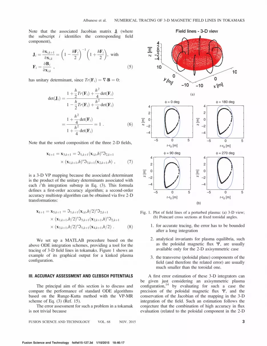
We set up a MATLAB procedure based on theabove ODE integration schemes, providing a tool for thetracing of 3-D field lines in tokamaks. Figure 1 shows anexample of its graphical output for a kinked plasmaconfiguration.

III. ACCURACY ASSESSMENT AND CLEBSCH POTENTIALS

The principal aim of this section is to discuss andcompare the performance of standard ODE algorithmsbased on the Runge-Kutta method with the VP-MRscheme of Eq. (3) (Ref. 15).

The error assessment for such a problem in a tokamakis not trivial because

1. for accurate tracing, the error has to be boundedafter a long integration

2. analytical invariants for plasma equilibria, suchas the poloidal magnetic flux Y, are usuallyavailable only for the 2-D axisymmetric case

3. the transverse (poloidal plane) components of thefield (and therefore the related error) are usuallymuch smaller than the toroidal one.

A first error estimation of these 3-D integrators canbe given just considering an axisymmetric plasmaconfiguration,14 by evaluating for such a case theprecision of the poloidal magnetic flux Y, and theconservation of the Jacobian of the mapping in the 3-Dintegration of the field. Such an estimation follows theconjecture that the combination of high accuracy in fluxevaluation (related to the poloidal component in the 2-D

(a)

–5 0 5

–4

–2

0

2

4

r-r0 [m]z

[m]

φ = 0 deg

–5 0 5

–4

–2

0

2

4

r-r0 [m]

z [m

]

φ = 180 deg

–5 0 5

–4

–2

0

2

4

r-r0 [m]

z [m

]

φ = 90 deg

–5 0 5

–4

2

4

r-r0 [m]

–2

0

z [m

]

φ = 270 deg

(b)

Fig. 1. Plot of field lines of a perturbed plasma: (a) 3-D view;(b) Poincare cross sections at fixed toroidal angles.

Albanese et al. NUMERICAL TRACING OF 3-D MAGNETIC FIELD LINES IN TOKAMAKS

FUSION SCIENCE AND TECHNOLOGY VOL. 68 NOV. 2015 3

Fusion Science and Technology fstfst15-127.3d 1/10/2015 18:46:17

axisymmetric case) with high volume preservation in the3-D integration guarantees good accuracy also forlongitudinal components.

Following such an approach, a DEMO configuration(plasma current Ip5 16 MA, major radius R05 9 m,minor radius a5 2.25 m, poloidal beta bp5 0.8, plasmainternal inductance li5 0.7, and toroidal field of 7 T at R0)is considered and B-field lines 1 km long within theplasma are traced16; then the considered algorithms aretested in terms of accuracy and computation time asfunctions of the integration step size in a cylindricalcoordinate system. Figure 2 shows the relative error interms of DY/Y, for different integration step lengths,whereas in Fig. 3 we illustrate the relative variation of theJacobian determinant as a function of the curvilinearabscissa over the field line. The observed periodicbehavior is explained for the axisymmetry of theconfiguration, after one complete turn in the poloidalplane is made. The local VP condition, |J|215 0, verifiedat the round-off error limit, stays within an accuracy of10210 for both the MR rule and the RK-IV scheme. Forthe latter, this gratifying result is mainly due to the smallintegration step selected for accuracy requirements.

Note that the relative error DY/Y in the evaluation ofthe magnetic flux scales with the integration step inperfect agreement with the algorithm order (Fig. 2), asproof that the considered integration step sizes are largeenough to consider round-off errors negligible withrespect to truncation error.

To evaluate the numerical accuracy in volumepreservation of the considered integration schemes, onehas to consider that the Jacobian matrix, Eq. (5), whoseentries consist of partial derivatives, can be numericallycalculated by a central-point derivation rule with a

second-order approximation. Therefore, the accuracy canbe evaluated with a second-order extrapolation as

JðtÞJð0Þ ¼ 2

Jh2

ðtÞJh2

ð0Þ2JhðtÞJhð0Þ þ O½h2� , ð9Þ

where J 5 det(Ji) is the Jacobian determinant and hindicates the step size for the numerical calculation of thepartial derivatives. As a result we get, for h5 320 mm, theaccuracies of |J|21 5 0 as 0.460 6 10–12 for MR and3.302 6 10–12 for RK-IV.

In Table I, a general comparison of the consideredalgorithms is given in terms of flux accuracy andcomputing time.

A fully 3-D tracing accuracy assessment can bedeveloped by observing that 3-D invariants can be foundusing the Clebsch decomposition for the magnetic fields.Such a representation expresses a divergence-free field asthe cross product of the gradients of two scalar functions as

B ¼ 7U £ 7V : ð10ÞThis representation is used in the description of themagnetic field lines as a Hamiltonian flow.17 In Eq. (10),the two Clebsch potentials U and V label magneticsurfaces (B?7U 5 0 and B?7V 5 0), so a magnetic fieldline is given by the intersection of two surfaces:U 5 constant and V 5 constant.

Using such fundamental properties, a first basicestimate of the accuracy in the numerical tracing of 3-Dmagnetic field lines can be obtained by evaluating therelative error on the U and V potentials along the tracedfield lines. To turn such information into a geometricalerror, it is possible to calculate the minimal distance

Fig. 3. Volume-preserving condition along the integration forMR and RK-IV at the truncation error limit.

35 17.5 8.74 4.36 2.1810–10

10–8

10–6

10–4

10–2

100

Integration Step [mm/T]

ΔΨ/Ψ

Relative Flux Accuracy

RK-IIMRRK-IV

Fig. 2. Flux accuracy in terms of integration step length for theconsidered algorithms: MR, RK-II, and RK-IV.

Albanese et al. NUMERICAL TRACING OF 3-D MAGNETIC FIELD LINES IN TOKAMAKS

4 FUSION SCIENCE AND TECHNOLOGY VOL. 68 NOV. 2015

Fusion Science and Technology fstfst15-127.3d 1/10/2015 18:46:17

kdPkmin between the exact field line U ¼ U0 > V ¼ V0

and the actual numerical line by solving in the least-squares sense the underdetermined set:

7U�dP ¼ U 2 U0

and

7V�dP ¼ V 2 V0 , ð11Þ

whereU and7U, and V and7V are the actual values of theClebsch potentials with their gradients at the points of thecomputed field line;U0 andV0 are the corresponding valuesof the Clebsch potentials on the analytical field line.

Considering the parametric equations of a toroidalhelix, we choose the Clebsch potentials in such a way thatthe corresponding field configuration resembles the fieldof a typical axisymmetric plasma:

U ¼ ðr2 R0Þ2a2

þ ðz2 Z0Þ2b2

þ U0

and

V ¼ u2w

qþ V0 , ð12Þ

where R0 and Z0 are the poloidal coordinates of the centerof the elliptic cross section of the helix, whose axes are aand b; q is the safety factor; w is the toroidal angle; u isobtained from ðr 2 R0Þ tanðuÞ ¼ z2 Z0 using the four-quadrant inverse tangent formula; and U0 and V0 arearbitrary constants.

Figure 4 shows two surfaces, U 5 constant andV 5 constant, defined by Eq. (12); their intersection is atoroidal helix confined inside the vacuum vessel.

Such an axisymmetric field configuration can beeasily modified by adding proper perturbing nonaxisym-metric terms in the expressions of U and V. In thefollowing, two kinds of perturbation will be considered,namely, a global perturbation and a local perturbation.

With regard to the global perturbation, a moderesembling the typical ripple field is given as

U ¼ ðr 2 R0Þ2ðaþ dUÞ2 þ

ðz2 Z0Þ2ðbþ dUÞ2 2 1 ,

dU ¼ dr cosðnwÞ ,and

V ¼ u2w

qþ V0 ð13Þ

and is shown in Fig. 5 for R0 5 9 m, Z0 5 0, a 5 0.75 m,b 5 1.25 m, q 5 2p, dr 5 0.25 m, and n 5 18.

TABLE I

Flux Accuracy for MR and RK with Respectto the Integration Step for an Integration

Length of 1000 m

Dt (mm/T) MR RK-II RK-IV

35.0DY (V?s) 0.911 1.382 5.986e24CPU time (s) 239 60 116

17.5DY (V?s) 0.225 0.346 3.907e25CPU time (s) 480 118 241

8.72DY (V?s) 0.057 0.087 2.492e26CPU time (s) 923 245 489

4.36DY (V?s) 0.014 0.022 1.574e27CPU time (s) 1594 493 990

2.18DY (V?s) 0.003 0.005 9.876e29CPU time (s) 2749 996 1992 Fig. 4. Clebsch surfaces generating a toroidal helix (the solid

line shows the intersection of the two surfaces).

Fig. 5. Ergodic surface covered by a field line in a globallyperturbed field configuration.

Albanese et al. NUMERICAL TRACING OF 3-D MAGNETIC FIELD LINES IN TOKAMAKS

FUSION SCIENCE AND TECHNOLOGY VOL. 68 NOV. 2015 5

Fusion Science and Technology fstfst15-127.3d 1/10/2015 18:46:19

Again, for the Jacobian conservation condition, we carryout the same extrapolation as for the axisymmetric test caseobtaining the accuracies for |J|21 5 0 as 0.4918 610–11

for the MR and 0.3190 610–11 for the RK-IV algorithms.For the local perturbation, we consider the following

(Fig. 6), obtained by adding a smooth function dU,Vp tothe unperturbed field:

U ¼ ðr 2 R0 2 dUÞ2a2

þ ðz2 Z0Þ2b2

2 1 ,

dU ¼ dr�e

a1Dz

2a1ffiffiffiffiffiffiffiffiffiffiffiffiffiffiffiffiffiffiffiffiffiffiffiffiffiffiffiffiffiffiffiffi

Dz2 2 ðZ1 2 zÞ2q

�e

a

Dw2

1ffiffiffiffiffiffiffiffiffiffiffiffiffiffiffiffiffiffiffiffiffiffiffiffiffiffiffiffiffiffiffiffiffiffiDw2 2 ðw1 2 wÞ2

quðr2 R0Þ in Vp

and 0 elsewhere ,

and

V ¼ u2w

qþ V0 , ð14Þ

with R05 9 m, Z05 0, a5 0.75 m, a15 10 m, b5 1.25 m,a 5 1 rad, q 5 2p, dr 5 1 m, Dz 5 0.5 m, X1 5 1.56 m,Y1 5 8.86 m, Z1 5 Z0, Dw 5 20 deg, w1 5 290 deg, and

Vp ¼jzj # z1

jw2 w1j # Dw

( ): ð15Þ

Table II shows the accuracy assessments both in theaxisymmetric and in the two full 3-D configurationsmentioned above, for the MR, RK-II, and RK-IV algorithms.

This analysis suggests that standard integrators, e.g.,Runge-Kutta, are extremely accurate in terms of volumepreservation (basically at the limit of round-off), whenselecting appropriate accuracy requirements (step size).At the same time, they are by far simpler and lessexpensive than VP algorithms from a computational point

Fig. 6. Ergodic surface covered by a field line for a locallyperturbed field configuration.

TABLEII

TracingAccuracy

forMRandRK

Estim

ated

UsingClebschPotentialsforan

IntegrationLength

of1000m

withaStepSizeof2.18mm/T

|U2U0|/U

0|V2V0|/V

0dP(m

)

Axisymmetric

Global

Perturbation

Local

Perturbation

Axisymmetric

Global

Perturbation

Local

Perturbation

Axisymmetric

Global

Perturbation

Local

Perturbation

MR

8.0e2

34.4e2

13e2

37.0e2

32.3e2

12.0e2

23.0e2

41.5e2

28.0e2

4RK-II

2.3e2

52.1e2

38.0e2

41.3e2

52.0e2

44.0e2

48.9e2

71.0e2

44.6e2

5RK-IV

2.1e2

12

4.3e2

81.0e2

71.1e2

11

2.0e2

95.3e2

96.9e2

13

4.0e2

95.5e2

9

Albanese et al. NUMERICAL TRACING OF 3-D MAGNETIC FIELD LINES IN TOKAMAKS

6 FUSION SCIENCE AND TECHNOLOGY VOL. 68 NOV. 2015

Fusion Science and Technology fstfst15-127.3d 1/10/2015 18:46:20

of view. Adaptive ODE solvers might be expected toshow better performance than fixed-step integrators interms of the trade-off between accuracy and computationtime; however, the use of step adaptivity may not preservespatial symmetries with drastic consequences.10

IV. APPLICATION TO PLASMA-WALL GAP CALCULATION

In this section, we determine the plasma-wall gap byevaluating 3-D field lines using the RK-IV scheme.

A practical way to reconstruct the plasma boundary ofgeneral 3-D field configurations is to define the connec-tion length as the length of the trajectory covered by theplasma particles over an entire magnetic field line up to itseventual intersection to the first wall, from a given startingpoint; the Larmor radius at this stage is simply neglected.The lines that never intersect the wall (periodic or ergodic)have infinite connection length and are by definitionwithin the plasma, whilst for a finite connection length,they have to be considered outside.18 By considering asufficiently dense grid of starting points, it is possible tomap the plasma boundary. The problem of tracing infinitelength lines can be practically circumvented by assumingthat a line is closed when it comes back within a givensmall distance from the initial point, or by defining amaximum admissible length much higher than expectedfor lines intersecting the wall.

Following such a connection length approach to thedefinition of the plasma boundary, we designed aprocedure that iteratively calculates the connection lengthfor successive initial positions along a given direction.Once a prescribed accuracy is assigned and a scanningstep defined with reference to the expected accuracy, theconnection length can be calculated along a segment, forinstance, in terms of the distance of the initial point fromthe wall.

We consider again the reference case as in Sec. III, withnow a kink perturbation of 2-deg rotation around the x-axisand a 5-cm shift along the same axis. Referring to such aplasma configuration, the connection lengths of 20 evenlyspaced lines were calculated along a radial direction on themidplane in the poloidal plane, from the first wall to theplasma edge, at w5 0 and w5 p. Figure 7a shows the r–zvalues of these field lines, with a blue color map for linesexternal to the plasma and red for the first internal line. Thecorresponding Poincare cross points are shown in Fig. 7b.

Figure 8 shows the connection length in terms of thedistance from the first wall for both the considered gaps; asharp transition from the external region to the plasmaregion is evident as well as the different distances where itoccurs, which is a consequence of the nonaxisymmetricfield configuration.

These results can be considered as a proof of principleof the viability of 3-D plasma boundary determination bymeans of accurate tracing of field lines and evaluation ofthe connection length. Strategies for an efficient use of

computing power can be easily implemented by consider-ing a bisection algorithm for the determination of theplasma-wall gap on the search direction. Parallel comput-ing is also suitable for concurrent calculation of severalsearch directions.19

V. CONCLUSIONS

We considered the problem of accurate tracing ofmagnetic field lines in tokamaks, where extremely long

(a)

(b)

Fig. 7. (a) Three-dimensional field lines in the r–z plane; (b)Poincare plots of the first internal line at w 5 0 (right)and w 5 p (left).

Albanese et al. NUMERICAL TRACING OF 3-D MAGNETIC FIELD LINES IN TOKAMAKS

FUSION SCIENCE AND TECHNOLOGY VOL. 68 NOV. 2015 7

Fusion Science and Technology fstfst15-127.3d 1/10/2015 18:46:20

lines with high local integration accuracy have to beevaluated. A VP ODE solver and standard RK routineswere validated and compared with the reference for aspecific problem. In particular, the error assessment wasconducted by means of analytical invariants, which for the2-D case are given by the constant poloidal flux values,and for the 3-D case by means of analytical expressionsbased on Clebsch potentials. Accuracy requirements aremet by both integration schemes if the integration stepsize is adequate. The volume preservation of the RK-IVscheme is comparable to that of the VP scheme whenusing the same step size, but the overall performance ofthe RK solver in terms of trade-off in accuracy andcomputational cost is by far higher than the VP scheme.As a result, standard fixed-step RK integrators are wellsuited to the problem and can be effectively used forB-field tracing in tokamaks. As a demonstration, plasma-wall gaps in a full 3-D configuration were calculated,showing the viability of studying the magnetic propertiesof plasma boundary in tokamaks using standard tools.

ACKNOWLEDGMENTS

This work was supported in part by the Italian Ministry ofEducation and Research under grant PRIN-2010SPS9B3. Theauthors gratefully acknowledge the contribution of A. Guarinoin the definition of some test cases.

REFERENCES

1. R. MAINGI et al., “Magnetic Field Line TracingCalculations for Conceptual PFC Design in the NationalCompact Stellarator Experiment,” Proc. XXXIII EPS Conf.,Rome, Italy, June 19–23, 2006.

2. M. W. JAKUBOWSKI et al., “Modelling of theMagnetic Field Structures and First Measurements of HeatFluxes for TEXTOR-DED Operation,” Nucl. Fusion, 44, S1(2004); http://dx.doi.org/10.1088/0029-5515/44/6/S01.

3. A. PUNJABI and H. ALI, “Symplectic Approach toCalculation of Magnetic Field Line Trajectories in PhysicalSpace with Realistic Magnetic Geometry in Divertor Toka-maks,” Phys. Plasmas, 15, 122502 (2008); http://dx.doi.org/10.1063/1.3028310.

4. F. MAVIGLIA et al., “Electromagnetic Models ofPlasma Breakdown in the JET Tokamak,” IEEE Trans.Magn., 50, 2, 937 (2014); http://dx.doi.org/10.1109/TMAG.2013.2282351.

5. M. SHOJI et al., “Investigation of the Helical DivertorFunction and the Future Plan of a Closed Divertor forEfficient Particle Control in the LHD Plasma Periphery,”Fusion Sci. Technol., 58, 1, 208 (2010); http://dx.doi.org/10.13182/FST10-04.

6. T. K. MAU et al., “Divertor Configuration and Heat LoadStudies for the ARIES-CS Fusion Plant,” Fusion Sci. Technol.,54, 3, 771 (2008); http://dx.doi.org/10.13182/FST08-27.

7. A. BRUSCHI et al., “A New Launcher for Real-TimeECRH Experiments on FTU,” Fusion Sci. Technol., 55, 1, 94(2009); http://dx.doi.org/10.13182/FST09-27.

8. B. D. BLACKWELL et al., “Algorithms for Real TimeMagnetic Field Tracing and Optimization,” Comput. Phys.Commun., 142, 243 (2001); http://dx.doi.org/10.1016/S0010-4655(01)00326-5.

9. R. I. McLACHLAN, G. REINOUT, and G. R. W.QUISPEL, “Geometric Integrators for ODEs,” J. Phys.A: Math. Gen., 39, 5251 (2006); http://dx.doi.org/10.1088/0305-4470/39/19/S01.

10. R. I. McLACHLAN and G. R. W. QUISPEL, “SixLectures on Geometric Integration,” Foundations of Com-putational Mathematics, R. DEVORE, A. ISERLES, andE. SULI, Eds., p. 155, Cambridge University Press,Cambridge (2001).

11. J. M. FINN and L. CHACON, “Volume PreservingIntegrators for Solenoidal Fields on a Grid,” Phys. Plasmas,12, 054503 (2005); http://dx.doi.org/10.1063/1.1889156.

12. D. BONFIGLIO et al., “Magnetic Chaos Healing in theHelical Reversed-Field Pinch: Indications from the Volume-Preserving Field Line Tracing Code NEMATO,” J. Phys. Conf.Ser., 260, 012003 (2010); http://dx.doi.org/10.1088/1742-6596/260/1/012003.

13. G. CIACCIO et al., “Numerical Verification of Orbitand Nemato Codes for Magnetic Topology Diagnosis,”Phys. Plasmas, 20, 062505 (2013); http://dx.doi.org/10.1063/1.4811380.

14. R. ALBANESE et al., “Numerical Formulations forAccurate Magnetic Field Flow Tracing in Fusion Tokamaks,”Proc. 9th IET Int. Conf. Computation in Electromagnetics,London, United Kingdom, March 31–April 1 (2014); http://dx.doi.org/10.1049/cp.2014.0211.

0 0.1 0.2 0.3 0.4 0.5102

102

103

Distance from the First Wall [m]

Line

Len

gth

[m]

Gap φ = 0

Gap φ = π

Fig. 8. Connection lengths versus the distance from the firstwall on the outboard equatorial plane z 5 0 at twodifferent toroidal locations (the integration stops after,2 km).

Albanese et al. NUMERICAL TRACING OF 3-D MAGNETIC FIELD LINES IN TOKAMAKS

8 FUSION SCIENCE AND TECHNOLOGY VOL. 68 NOV. 2015

Fusion Science and Technology fstfst15-127.3d 1/10/2015 18:46:21

15. J. R. DORMAND and P. J. PRINCE, “A Family ofEmbedded Runge-Kutta Formulae,” J. Comput. Appl. Math., 6,19 (1980); http://dx.doi.org/10.1016/0771-050X(80)90013-3.

16. G. FEDERICI et al., “Overview of EU DEMO Design andR&D Activities,” Fusion Eng. Des., 89, 7–8, 882 (2014); http://dx.doi.org/10.1016/j.fusengdes.2014.01.070.

17. S. V. BULANOV et al., “Current Sheet Formation inThree-Dimensional Magnetic Configurations,” Phys. Plasmas,9, 3835 (2002); http://dx.doi.org/10.1063/1.1501093.

18. M. ITAGAKI et al., “Use of a Twisted 3D CauchyCondition Surface to Reconstruct the Last Closed MagneticSurface in a Non-Axisymmetric Fusion Plasma,” Plasma Phys.Controlled Fusion, 54, 125003 (2012); http://dx.doi.org/10.1088/0741-3335/54/12/125003.

19. R. TSUJI, “Parallel Computing for Tracing Torus MagneticField Line,” Proc. Int. Conf. Parallel Computing in ElectricalEngineering, Trois-Rivieres, Quebec, Canada, August 27–30,2000, IEEE (2000).

Albanese et al. NUMERICAL TRACING OF 3-D MAGNETIC FIELD LINES IN TOKAMAKS

FUSION SCIENCE AND TECHNOLOGY VOL. 68 NOV. 2015 9

Fusion Science and Technology fstfst15-127.3d 1/10/2015 18:46:21