Embed Size (px)
Citation preview

ORIGINAL ARTICLE
Acoustic thoracic image of crackle sounds using linearand nonlinear processing techniques
Sonia Charleston-Villalobos • Guadalupe Dorantes-Mendez •
Ramon Gonzalez-Camarena • Georgina Chi-Lem • Jose G. Carrillo •
Tomas Aljama-Corrales
Received: 21 January 2010 / Accepted: 4 July 2010 / Published online: 21 July 2010
� International Federation for Medical and Biological Engineering 2010
Abstract In this study, a novel approach is proposed, the
imaging of crackle sounds distribution on the thorax based
on processing techniques that could contend with the
detection and count of crackles; hence, the normalized
fractal dimension (NFD), the univariate AR modeling
combined with a supervised neural network (UAR-SNN),
and the time-variant autoregressive (TVAR) model were
assessed. The proposed processing schemes were tested
inserting simulated crackles in normal lung sounds
acquired by a multichannel system on the posterior thoracic
surface. In order to evaluate the robustness of the pro-
cessing schemes, different scenarios were created by
manipulating the number of crackles, the type of crackles,
the spatial distribution, and the signal to noise ratio (SNR)
at different pulmonary regions. The results indicate that
TVAR scheme showed the best performance, compared
with NFD and UAR-SNN schemes, for detecting and
counting simulated crackles with an average specificity
very close to 100%, and average sensitivity of 98 ± 7.5%
even with overlapped crackles and with SNR correspond-
ing to a scaling factor as low as 1.5. Finally, the perfor-
mance of the TVAR scheme was tested against a human
expert using simulated and real acoustic information. We
conclude that a confident image of crackle sounds distri-
bution by crackles counting using TVAR on the thoracic
surface is thoroughly possible. The crackles imaging might
represent an aid to the clinical evaluation of pulmonary
diseases that produce this sort of adventitious discontinu-
ous lung sounds.
Keywords Discontinuous adventitious sound imaging �Lung sound � Fine and coarse crackles � Time-variant
autoregressive model � Fractal dimension
1 Introduction
Physicians use the classical auscultation procedure on the
chest wall to look for peculiar lung sounds (LS), breathing
and adventitious sounds, to diagnose lung disorders [30].
However, the findings are biased by the physician’s
expertise to correctly identify diverse adventitious sounds
[21]. Furthermore, the classical auscultation is performed
using a single stethoscope at different positions on the
thoracic surface, and the physician needs to integrate in a
qualitative way the whole spatial and temporal acoustic
information to reach a diagnosis. Several pulmonary dis-
orders are described by the occurrence of discontinuous
adventitious LS, also known as crackles, that depending on
the severity of the disease the physicians are capable to
perceive [28]. It is accepted that to know the extent of the
pulmonary area where crackles are occurring is clinically
important [31]. Therefore, providing a confident image of
the spatial distribution of the pulmonary pathology by
detecting and counting crackles using multiple acoustic
sensors might help to overcome the restrictions of the
clinical auscultation with the stethoscope.
S. Charleston-Villalobos (&) � G. Dorantes-Mendez �T. Aljama-Corrales
Department of Electrical Engineering, Universidad Autonoma
Metropolitana, Mexico City 09340, Mexico
e-mail: [email protected]
R. Gonzalez-Camarena
Department of Health Science, Universidad Autonoma
Metropolitana, Mexico City 09340, Mexico
G. Chi-Lem � J. G. Carrillo
National Institute of Respiratory Diseases, Mexico City 14080,
Mexico
123
Med Biol Eng Comput (2011) 49:15–24
DOI 10.1007/s11517-010-0663-5

Murphy et al. [26] and then Hoevers and Loudon [14]
have described crackles through their time-expanded
waveform-analysis (TEWA), defining by visual inspection
time parameters as the initial deflection width (IDW), the
two cycle duration (2CD) and the largest deflection width
(LDW). Based on TEWA, fine and coarse crackles were
differentiated and associated to different pathologies [1].
Mori et al. [24] and Munakata et al. [25] studied crackle
sounds in the frequency domain and reported crackle
spectral content mainly in the range from 0.1 to 1000 Hz.
In particular, crackle sounds have been associated to both
cardiac and pulmonary diseases [29]. Furthermore, fine and
coarse crackles have been reported appearing during
inspiration and expiration phases, depending on the pul-
monary disorder. In fibrotic lung diseases, as it occurs in
many parenchymal lung diseases, fine crackles are more
frequently found at the ending of the inspiratory phase [29].
Several efforts have been made to automatically detect
fine and coarse crackles. Among such techniques are non-
linear digital filters [27], the spectral stationarity of LS [15],
high-order statistics AR modeling [10], wavelet transform
[11], neurofuzzy modeling [32], fractal dimension [12], the
empirical mode decomposition [3, 8], and recently a texture-
based classification [9]. Nevertheless, the solution for auto-
mated crackle detection remains as a challenging research
area due to factors such as: (a) non-stationarity behavior of
crackle and breathing sounds (BS), (b) the signal-to-noise
ratio (SNR) between crackle and BS, (c) temporal crackles
overlapping, (d) crackle waveform distortion by BS, and (e)
the task complexity in a multichannel scenario due to tem-
poral and spatial changes of crackle and BS characteristics. It
is interesting to note that most of the actual studies related to
crackles utilize the counting obtained by clinical experts
using TEWA to validate the results. However, it has been
shown that physicians have visual and auditory limitations to
detect fine or coarse crackles [17]. Here, we hypothesize that
2D imaging of crackles distribution on the thoracic surface is
feasible by processing multichannel acoustic information.
The 2D image modality has the advantage to be non-invasive
and related to the function of the lung. Besides, the meth-
odology can be applied to image other kind of adventitious
LS, as wheezes or squawk sounds.
The aim of this article is to propose a novel concept, the
imaging of crackle sounds to determine their spatial dis-
tribution, and the estimated number of crackles using linear
and non-linear processing schemes in a multichannel
framework.
2 Methodology
The methodology for imaging crackles or discontinuous
adventitious LS is depicted in Fig. 1. In order to construct a
simulated database controlling the extent of the abnormal
pulmonary zones, the SNR, the type, and the number of
crackles, a multichannel LS acquisition from healthy sub-
jects, was carried out. Afterward, simulated fine and coarse
crackles were inserted in normal breathing LS by an
additive model. As can be seen in Fig. 1, three schemes
were proposed to estimate and count the number of
crackles based on the normalized fractal dimension (NFD),
the univariate autoregressive modeling combined with a
supervised feedforward neural network (UAR-SNN), and
the time variant autoregressive modeling (TVAR). Finally,
the image of crackle sounds distribution was formed using
the estimated number of crackles or the mapping of a
crackling index.
2.1 Normal breathing (basic) LS and preprocessing
stage
The acquisition protocol was carried out at the Digital
Signal and Image Processing Laboratory of the Metropol-
itan Autonomous University in collaboration with the
Acoustic Laboratory of the National Institute of Respira-
tory Diseases, at Mexico City. Multichannel LS signals
were acquired from 10 healthy subjects with an average
age, weight, and height of 24.3 ± 1.5 years, 77.8 ± 11.0 kg,
and 174.8 ± 7.8 cm, respectively, who signed an informed
consent according to Helsinki guidelines. The sensor array
of 5-by-5, attached to the subject’s posterior thoracic sur-
face, consisted of electret microphones inserted in plastic
bells with a flat frequency response from 50 Hz to 3 kHz.
Nomenclature of the sensor array is described in detail
elsewhere [2, 3]. During the acquisition, the subjects were
seated, breathing through a calibrated type Fleisch pneu-
motachometer at airflow of 1.5 l s-1, and wearing a nose
clip; the acquisition session lasted 15 s with initial and final
apnea phases of 5 s. In order to digitize the multichannel
LS and airflow signals, a 12-bit A/D converter was used
with a sampling frequency of 10 kHz. LS signals were
processed by band pass filtering with cutoff frequencies of
75 and 1,000 Hz; the lower cutoff frequency was selected
to attenuate heart sounds interference. In this study, only
inspiratory phases were used and segmented by the airflow
signal as reference signal.
2.2 Simulation of abnormal LS and pattern images
In order to simulate different spatial distributions of
abnormal LS, mathematically simulated crackles (SCs)
were embedded by an additive model within the acquired
normal breathing LS signals from 10 healthy subjects. Two
crackle types were simulated using the mathematical
function proposed by Kiyokawa et al. [17], which is
16 Med Biol Eng Comput (2011) 49:15–24
123
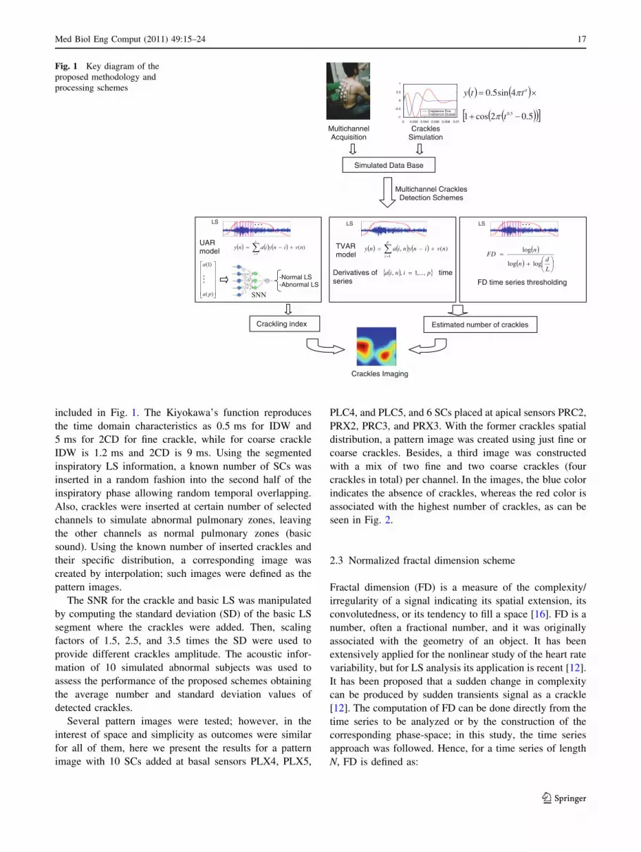
included in Fig. 1. The Kiyokawa’s function reproduces
the time domain characteristics as 0.5 ms for IDW and
5 ms for 2CD for fine crackle, while for coarse crackle
IDW is 1.2 ms and 2CD is 9 ms. Using the segmented
inspiratory LS information, a known number of SCs was
inserted in a random fashion into the second half of the
inspiratory phase allowing random temporal overlapping.
Also, crackles were inserted at certain number of selected
channels to simulate abnormal pulmonary zones, leaving
the other channels as normal pulmonary zones (basic
sound). Using the known number of inserted crackles and
their specific distribution, a corresponding image was
created by interpolation; such images were defined as the
pattern images.
The SNR for the crackle and basic LS was manipulated
by computing the standard deviation (SD) of the basic LS
segment where the crackles were added. Then, scaling
factors of 1.5, 2.5, and 3.5 times the SD were used to
provide different crackles amplitude. The acoustic infor-
mation of 10 simulated abnormal subjects was used to
assess the performance of the proposed schemes obtaining
the average number and standard deviation values of
detected crackles.
Several pattern images were tested; however, in the
interest of space and simplicity as outcomes were similar
for all of them, here we present the results for a pattern
image with 10 SCs added at basal sensors PLX4, PLX5,
PLC4, and PLC5, and 6 SCs placed at apical sensors PRC2,
PRX2, PRC3, and PRX3. With the former crackles spatial
distribution, a pattern image was created using just fine or
coarse crackles. Besides, a third image was constructed
with a mix of two fine and two coarse crackles (four
crackles in total) per channel. In the images, the blue color
indicates the absence of crackles, whereas the red color is
associated with the highest number of crackles, as can be
seen in Fig. 2.
2.3 Normalized fractal dimension scheme
Fractal dimension (FD) is a measure of the complexity/
irregularity of a signal indicating its spatial extension, its
convolutedness, or its tendency to fill a space [16]. FD is a
number, often a fractional number, and it was originally
associated with the geometry of an object. It has been
extensively applied for the nonlinear study of the heart rate
variability, but for LS analysis its application is recent [12].
It has been proposed that a sudden change in complexity
can be produced by sudden transients signal as a crackle
[12]. The computation of FD can be done directly from the
time series to be analyzed or by the construction of the
corresponding phase-space; in this study, the time series
approach was followed. Hence, for a time series of length
N, FD is defined as:
Derivatives of time series
UARmodel
L
dn
nFD
loglog
log)(,1
nvinynianyp
i
)(1
nvinyianyp
i
SNN
pinia ,...,1,,
)(
)1(
pa
a
-Normal LS -Abnormal LS
LS LS LS
FD time series thresholding
TVARmodel
…
…
MultichannelAcquisition
Crackles Simulation
Simulated Data Base
0 0.002 0.004 0.006 0.008 0.01-1
-0.5
0
0.5
1
Crepitancia FinaCrepitancia Gruesa
Multichannel Crackles Detection Schemes
5.02cos1
4sin5.0
5.0t
tty
…
Estimated number of cracklesCrackling index
Crackles Imaging
Fig. 1 Key diagram of the
proposed methodology and
processing schemes
Med Biol Eng Comput (2011) 49:15–24 17
123

DF ¼ log Lð Þlog dð Þ;
where L is the total length of the signal, calculated as the
sum of all the distances between any two consecutive
points, and d corresponds to the diameter or planar extend
of the signal, calculated as the maximum distance between
the starting point and any other point in the signal. In order
to avoid the dependency of FD on signal’s units, we use the
normalized fractal dimension (NFD) version, Fig. 1, given
by:
NFD ¼ log nð Þlog nð Þ þ log d=Lð Þ;
where n = N - 1. Each inspiratory phase was divided into
99% overlapping temporal windows of length 0.006 times
the sampling frequency in accordance to other authors [12].
The NFD was calculated for each temporal window in the
second half of the inspiratory phase. Afterward, the esti-
mated number of crackles was obtained for each channel
by testing different threshold values on the NFD time series
and then a matrix of 5-by-5 was formed with the estimated
values. Finally, the matrix was interpolated by the Hermite
function to form the crackle sounds image.
2.4 Univariate AR modeling-SNN scheme
A stationary random process can be modeled as the output
of a time invariant linear all-pole filter excited by white
noise as follows:
u½n� ¼ �a1u½n� 1� � a2u½n� 2�. . .� apu½n� p� þ v½n�;
where u[n], the actual sample of the process, is represented
by a lineal combination of its p previous samples and the
actual sample of the error signal. The univariate autore-
gressive (UAR) model involves second-order statistical
information of the stationary process [19] and the param-
eters {ai, i = 1,…,p}, so as the model order p, need to be
determined. Burg’s algorithm was used to estimate the AR
coefficients, and the Akaike criterion was employed to
select the order of the AR model. It is assumed that normal
and abnormal LS are characterized by different sets of AR
coefficients representing two different classes in the feature
space.
In order to classify acoustic information as being normal
(absence of crackles) or abnormal (presence of crackles) by
a SNN, each inspiratory phase was segmented into 30
windows overlapped by 25% [22]. According to the Akaike
criterion, a sixth-order UAR model was obtained for each
6 6
6 6
10 10
10 10
6 6
6 6
9 9
9 9
6 7
6 6
10 10
10 10
5 6
5 5
10 10
9 10
1 1
2 1
4
1 1
2 3 1
1 4
1
1
3 6 1
2 2 4
26 26
26 26
48 48
48 48
33 33
33 33
46 45
46 46
30 30
30 30
54 54
54 54
TVAR NFD UAR-SNN
PATTERN IMAGE
(a) (b) (c)
Fig. 2 Estimated images for
fine simulated crackles
detection using a univariate
autoregressive model-neural
network scheme (UAR-SNN),
b normalized fractal dimension
scheme (NFD), and c time
variant autoregressive model
scheme (TVAR) for the three
scaling factors 1.5, 2.5, and 3.5,
from top to bottom, respectively
18 Med Biol Eng Comput (2011) 49:15–24
123

temporal window, Fig. 1, providing 30 feature vectors of
length 6 for each inspiratory phase and for each channel.
The SNN architecture was defined with two hidden layers;
the number of hidden nodes was varied from 5 to 30, until
the best performance was obtained according to the mean
squared error (MSE). Finally, a SNN with two hidden
layers having 20 and 10 neurons, and a single output unit
was applied for classification purpose. For adjusting the
SNN’s weights, the supervised training algorithm used the
hyperbolic tangent sigmoid function and the gradient-
descendent Levenberg–Marquardt method [7]. Besides,
each temporal window of the training data set was labeled
as normal or abnormal according to the position and
duration of the SCs. The temporal window was labeled as 1
for normal and -1 for abnormal condition. The simulated
database was divided in training (80% of database), vali-
dation (10% of database), and testing data (10% of data-
base). For the case of UAR-SNN scheme, we propose the
crackling index to indicate the relevance of crackle sounds
by the ratio:
Crackling index
¼ Number of windows classified as abnormal
Number of windows classified as normal� 100;
where a temporal window was classified as normal if the
SNN output node value was C0.8. Otherwise, if SNN
output was B-0.8, the information was labeled as abnor-
mal. The crackling index was obtained for each inspiratory
phase, represented by 30 feature vectors, for each one of
the 25 channels. Finally, the crackle image was formed
interpolating the 25 crackling index values by the Hermite
function.
2.5 Time variant AR model scheme
The time variant autoregressive (TVAR) model is proposed
to estimate the number of crackles by accounting for
temporal non-stationary changes produced by the occur-
rence of crackles. The TVAR model is given by:
Xp
i¼0
a�i ðnÞu n� kð Þ ¼ v nð Þ;
where the AR coefficients {ai(n), i = 1,…,p} are calcu-
lated sample by sample. The TVAR coefficients were
obtained by the recursive least squares (RLS) algorithm
minimizing the cost function n(n) =P
i=1n kn-i|e(i)|2,
where k represents the forgetting factor, and e(i) = u(i) -
y(i) is the error signal in terms of the output of the adaptive
filter that depends on the past values of u(n) [13]. The
forgetting factor, k [ (0, 1), controls the influence of prior
information on which the cost function is minimized, i.e.,
with a small k value the RLS algorithm has short memory
length, being more sensitive to recent samples. For crackle
detection, k = 0.97 was found to be adequate for tracking
sudden nonstationary changes by the RLS algorithm,
allowing a confident count of the crackles into the basic
LS. Although the forgetting factor can be determined
adaptively, this approach was not explored here. The order
of TVAR model, for all the channels, was fixed at four.
In addition, we propose a criterion to decide the pres-
ence of a crackle based on the abrupt changes in the
derivative of the TVAR coefficient time series. A thres-
holding procedure was applied to the four derivatives and
only if an abrupt change was above the threshold in the
four time series the information was considered as pro-
duced by a crackle. For all the scaling factors, a threshold
of 0.035 times the standard deviation of the derivatives of
the AR coefficient time series was empirically established.
The estimated number of crackles for each channel was
interpolated by the Hermite function and a discontinuous
adventitious sounds image was constructed.
2.6 Processing schemes assessment
The processing schemes were evaluated by their ability to
detect the simulated abnormal regions of the lung in
accordance with the estimated number of inserted SCs. The
robustness of the processing schemes was achieved fol-
lowing two approaches: (a) controlling the SNR, the
number of crackles, their timing in the inspiratory phase
and their spatial distribution and (b) contrasting the results
against the performance of a human expert to detect by
TEWA simulated and real crackle sounds.
3 Results
3.1 Influence of SNR on crackles morphology
A factor that influences the performance of almost any
signal detection scheme is the SNR between the desired
signal and the background noise. In order to visually cor-
roborate the influence of the basic LS on crackles mor-
phology, Fig. 3 shows fine SCs embedded in LS signals at
sensors PRC2 and PLX4, using scaling factors 1.5 and 3.5.
The arrows at the top of each signal point out the precise
temporal position of the SCs. Analyzing the signal’s mor-
phology with factor 1.5 in Fig. 3a, it is easy to conclude
that some crackles were barely visible and even lost the
TEWA criterion. On the other hand, and knowing in
advance their temporal position, visual recognition of some
crackles was relatively easy with a factor 3.5, Fig. 3b.
However, the morphology of the sixth embedded crackle
looks severely modified by the surrounding basic LS
increasing the difficulty to detect it even by a specialist.
Med Biol Eng Comput (2011) 49:15–24 19
123

Also, crackles’ morphology was severely distorted as the
crackles were in closer sequence or overlapped, as can be
seen for the first and second crackles in Fig. 3b.
3.2 Estimated images for fine SCs using UAR-SNN
scheme
In Fig. 2, the simulated pattern image for fine crackles is
shown at the center of the first column. The three estimated
images by the UAR-SNN scheme for scale factors 1.5, 2.5,
and 3.5 are shown, from top to bottom, in the second column
of Fig. 2; the color bar is related to the proposed crackling
index. The SNN’s weights were adjusted by considering the
acoustic information of each channel independently, and the
sensitivity obtained in the training phase, for the three scaling
factors, was between 98.6 and 99.1%, while the specificity
was between 95.3 and 96.8%. In the estimated images, there
were two well-defined zones and, more important, they were
associated with the crackle number used to synthesize the
pattern image. The estimated image for the scale factor 3.5
was the closest to the pattern image due to the highest SNR.
Furthermore, even with the lowest scale factor 1.5, it is
possible to recognize two regions containing different
number of crackles in the estimated image. Due to the fact
that the inspiratory phase was divided in 30 segments and the
crackles were inserted in its second half, the crackling index
values 54 and 30 correspond to 10.8 and 6 abnormal temporal
windows, respectively. Certainly, if the number of crackles is
unknown, crackles relevance in the estimated image needs to
be evaluated according to the intensity of the colored area on
the thorax. An extension of the former results is shown in
Fig. 4a, where the image was constructed by averaging the
estimated number of crackles for the 10 simulated abnormal
subjects and for the more critical scaling factor of 1.5.
3.3 Estimated images for fine SCs using NFD scheme
In Fig. 2, and using as reference the same simulated pattern
image, the third column presents the results for the NFD
scheme. In this case, the color bar values represent the
estimated number of crackles. As can be observed in the
estimated image for the scaling factor 3.5, there was a
single zone at the left thoracic base, coinciding with the
image pattern, but the estimated number of crackles was
highly underestimated. The results from the 10 subjects are
not shown here as the NFD scheme gave a very low per-
formance for all the scaling factors.
3.4 Estimated images for fine SCs using TVAR scheme
The results by TVAR are shown in the fourth column of
Fig. 2, where the color bar represents, as for the NFD
scheme, the estimated number of crackles. It is evident that
for the three scaling factors there was a good estimation of
the number of fine crackles, and consequently, the esti-
mated crackle images were in good agreement with the
pattern image. For the 10 simulated abnormal subjects, the
image formed by averaging the estimated crackles is pre-
sented in Fig. 4b, for the scaling factor 1.5. As can been
seen, the estimated average number of crackles was very
close to the number of inserted crackles in the pattern
image with standard deviation lower than 1.0. It is worthy
to note that for the remaining channels, where crackles
were not inserted, the TVAR scheme did not detect the
presence of any crackle. Finally, the average specificity
was very close to 100% and the average sensitivity was
98 ± 7.5%, even with overlapped crackles and with SNR
corresponding to a scaling factor as low as 1.5.
3.5 Estimated images for coarse SCs by TVAR scheme
In case of coarse crackles, all the schemes were also
evaluated. However, here we highlight the results for
TVAR as this scheme gave the best performance for all the
scaling factors and it does not require training for the dif-
ferent simulated scenarios as the UAR-SNN scheme does.
Figure 5 provides the estimated images for the scaling
factors 1.5, 2.5, and 3.5, and the color bar represents the
4.7 4.75 4.8 4.85 4.9 4.95 5 x 10⁴
-10
0
10 ↓ ↓↓ ↓↓ ↓
4.6 4.65 4.7 4.75 4.8 4.85 4.9 x 10⁴
-20 -10
0 10 ↓↓ ↓ ↓↓↓
Samples
Am
plit
ude
(m
V)
Fig. 3 Embedded fine crackles for scaling factors 1.5 (upper signal)and 3.5 (lower signal), arrows point out crackles’ temporal position
25.6±3.0
25.4 ±3.4
25.7±2.6
25.4 ±3.3
39.5 ±4.7
39.4 ±5.1
40.0 ±4.8
40.0 ±4.9
5.6
±0.75.9
±0.6
5.7
±0.55.8
±0.4
9.8 ±0.8
9.8 ±0.8
9.8 ±0.8
9.7 ±0.7
(b) (a)
Fig. 4 Estimated average images for ten subjects using fine
simulated crackles and scaling factor 1.5; a crackling index
(mean ± SD) by UAR-SNN and b crackles number (mean ± SD)
by TVAR schemes
20 Med Biol Eng Comput (2011) 49:15–24
123

number of estimated crackles. The TVAR scheme could
fairly identify the coarse crackle zones for the three scaling
factors, and the estimated number of crackles was very
close to the pattern image of Fig. 2.
3.6 Estimated images for combined fine and coarse
SCs using TVAR scheme
The estimated image by the TVAR for the pattern image in
Fig. 6a, using the scaling factor 1.5, is shown in Fig. 6b.
The result indicates the robustness of the TVAR scheme to
detect fine and coarse crackles as the four inserted crackles
were detected and counted at the right positions.
3.7 Estimated number of fine SCs by TVAR scheme
and the expert
Figure 7 depicts the images derived from detection and
counting of simulated crackles with a scaling factor 3.5 by
the TVAR scheme, Fig. 7a, and by a human expert using
TEWA criteria, Fig. 7b. It can be observed that the expert
had an approximation to the simulated abnormal regions
where the crackles were inserted, but crackles’ counting
was deficient. We corroborated that some crackles were
overlapped and some others were of too low amplitude, so
that detecting them by the expert was very difficult.
3.8 Estimated number of real crackles by TVAR
scheme and the expert
Finally, the performance of TVAR scheme was analyzed
on real acquired LS signals from patients with diagnosis of
idiopathic pulmonary fibrosis (IPF) and compared with the
crackle counting estimation by the expert using TEWA
criteria and listening skill. The IPF is a diffuse parenchy-
mal lung disease of difficult diagnosis and management,
usually leading to relatively short half-life after the diag-
nosis is established. Acoustical information from two IPF
patients with evident large amplitude crackles was used to
facilitate crackles identification by the physician; the
patients suffered dyspnea, cough, pulmonary restrictive
pattern, oxygen desaturation during exercise, and the high
resolution computed tomography (HRCT) showed bilateral
ground-glass with some honeycombing pattern. The
acoustic information was acquired with the patients
breathing at 1.5 l s-1. Figure 8a presents the LS signal
containing crackles from one of the patients. It can be seen
in the time expanded waveform, Fig. 8b, that the amplitude
of the crackles was high enough to visually identify them
matching the TEWA criteria. For the first patient, the
crackle counting was performed for seven inspiratory
phases, Table 1. In average, the TVAR scheme obtained
(a) (b)
(c)
6 7
6 6
10 10
10 10 1
5 6
5 5
10 10
9 9 1
6 6
6 6
10 11
10 11
Fig. 5 Estimated images by detecting and counting coarse crackles
using TVAR scheme; a scaling factor 1.5, b scaling factor 2.5, and
c scaling factor 3.5
(a) (b)
4 4
4 4
4 4
4 4
4 4
4 4
4 5
4 4
Fig. 6 Detection for mixed fine and coarse crackles by TVAR:
a pattern image including four fine and four coarse crackles and
b estimated image
5 4
2 2
0 3
4 5
6 6
6 6
10 10
9 9
(a) (b)
Fig. 7 Crackles’ counting comparison between TVAR and medical
expert in one ‘‘sick’’ subject: a estimated image by TVAR, b estimated
image by expert
Med Biol Eng Comput (2011) 49:15–24 21
123

5.7 crackles, while the expert counted 6.0 crackles. For the
second patient, using six inspiratory phases, TVAR scheme
estimated 3.2 crackles and the expert 3.0 crackles. The
results show that for the two patients, due to the high SNR,
the expert was able to identify and count the number of
crackles and, most important, his performance was in
agreement with the estimation of the TVAR scheme.
4 Discussion
X-ray, tomography, MRI, and other techniques for medical
imaging are currently applied almost in all the medical
fields. Furthermore, visualization of anatomical and func-
tional abnormal zones of the pulmonary fields is the focus
of considerable research. The acoustic imaging of the
thorax has been suggested and explored based on non-
simultaneous and simultaneous multichannel approach.
The acoustical imaging has been developed in two ways; in
the first approach, the focus was on determining breathing
sounds energy distribution on the surface of the thorax, as
an estimation of regional ventilation [6]. Accordingly, in
2004, Charleston et al. [2] encouraged the use of the
respiratory acoustic thoracic imaging (RATHI) to analyze
lung sound origin, spatial distribution, frequency content,
and relationship to ventilation in both healthy and ill sub-
jects. In addition, the same study included the visual cor-
relation between the acoustical image and the X-ray of a
patient to show the potentiality of the mapping of multi-
channel LS intensities. Further, since 2007, other authors
reported studies with some clinical applications of the LS
intensity acoustic image using the Vibration Response
Imaging system [4, 5, 23]. In the second approach, the
research was centered on the estimation of sound sources
within the thorax in an effort to reconstruct airway geom-
etry [18]. However, the second approach has been less
explored and no current clinical applications are derived. In
contrast with the former efforts and as an alternative in
providing additional information to the physician, in the
present work instead of mapping the intensity of LS we
propose the mapping of crackles sounds detecting and
counting them to get their relevance. It can be thought that
the crackle image is a kind of functional imaging associ-
ated with the number of abnormally closed airways that
could evidence the extent of the associated pulmonary
disease. The proposed image overcomes restrictions of the
conventional auscultation procedure where subjectivity and
non-controlled settings are common.
To establish the new concept of crackle imaging simu-
lating different scenarios represents an advantage to deal
with morphological changes of crackles due to the back-
ground LS. Besides, working with simulated scenarios is
relevant when a gold standard is not available. This
approach is one of the strengths of the present work as a
thorough control of the number, type, amplitude, and
timing of crackles was achievable. With real cases, such
control would be unfeasible since the TEWA criteria show
important limitations to identify correctly crackles when
they are overlapping or they have low amplitude. In this
article, the simulated scenarios allowed us to show that it is
feasible to automatically detect low amplitude crackles that
the physician missed using the TEWA criteria. The
robustness of the selected processing schemes was assessed
including both hemithorax using simulated cases and real
signals from two patients.
Our main findings pointed out that in contrast to the
human expert, simulated fine and coarse crackles with low
SNR and overlapped can be detected by UAR-SNN and
TVAR schemes, so that an automated and confident image
representing the spatial distribution of crackles was thor-
oughly possible. It should be considered that one of the
fundamental assumptions in this study was that crackle
sounds are added to the basic LS.
For many years, it has been accepted that crackle sounds
have a well-defined waveform. In fact, Murphy et al. [26]
gave the first description of the amplitude and time
5.64 5.66 5.68 5.7 5.72
-5
0
5
10
Samples
(b)
Am
plitu
de
(mV
)
X 1044 4.5 5 5.5 6 6.5 7
-20
-10
0
10
20
X 104
(a)
Fig. 8 a Acquired real LS signal from an IPF patient with five
inspiratory phases and b time-waveform expansion of the third
inspiratory phase
Table 1 Crackles’ counting by TVAR scheme and expert for real LS
signals
Mean ± SD
TVAR Expert
Patient 1 (n = 7 inspiratory phases) 5.7 ± 1.1 6.0 ± 1.0
Patient 2 (n = 6 inspiratory phases) 3.2 ± 1.9 3.0 ± 1.7
TVAR time variant autoregressive model, LS lung sounds
22 Med Biol Eng Comput (2011) 49:15–24
123

characteristics of crackles (TEWA), suggesting some spe-
cific criteria for their visual detection and parametrization.
Among the suggested characteristics, they pointed out that
amplitude of convincing crackles should be twice the
amplitude of the surrounding LS. However, in a recent
paper of the same group, they gave evidence that crackles
waveform shows some inconsistencies that made difficult
the parametrization of crackles by TEWA [34]. Our results
agree with such observation, as many of the simulated
crackles inserted in basic LS lost their morphology and lost
the conditions to be accepted as a factual crackle, more
even when they are overlapped. On the other hand, in the
same study, Vyshedskiy et al. [34] offer evidences that
support the stress-relaxation quadrupole theory, so that
based on the mechanism of generation of inspiratory and
expiratory crackles these authors explain the crackle’s
morphology. However, it is expected that the amplitude
and general morphology of crackles recorded at the tho-
racic surface depend on the mechanism of generation (i.e.,
transpulmonary pressure), the source’s depth, the trans-
mission properties of the pulmonary structure, and the
presence of destructive and constructive waves. Therefore,
the waveform of crackles recorded on the thoracic surface
may not always hold the TEWA criteria. This is extremely
important because if we use the TEWA criteria we might
be missing many crackles that are of low amplitude and do
not cover the defined deflections. Thus, instead of ampli-
tude and temporal parameters, we choose schemes based
on different parameterizations to estimate low amplitude
and random temporal overlapping crackles.
Although NFD scheme has been suggested by some
authors for detecting and counting real crackles [12], the
results were dependent on the crackles’ amplitude. Our
findings indicate that the NFD scheme was unable to
contend with a scaling factor of 3.5 even applying different
threshold values to the NFD time series, and consequently,
this technique alone could be not enough for this applica-
tion. On the other hand, UAR-SNN and TVAR schemes
seem encouraging for automated detection and counting
fine and coarse crackles even with amplitudes below two
times the amplitude of the surrounding basic LS. Even
though the abnormal regions were rightly detected by both
schemes, at this moment the detection and counting of
factual crackles can be assured only for the TVAR scheme
that even contended with the lowest simulated SNR and
with randomly overlapped crackles. A feasible reason of
the TVAR model performance over the UAR model may
be related to the fact that each time sample is modeled by
four coefficients in comparison with six UAR coefficients
used for all the samples included in each time window. In a
future work, it could be interesting to assess the perfor-
mance of both time variant and invariant AR model using
algorithms to rank the importance of the model coefficients
as stated by Zou et al. [35] and Lu et al. [20] and reported
to provide better results than either RLS or Burg’s algo-
rithms. Furthermore, it could be relevant to determine the
most significant coefficients for different respiratory
pathologies associated with different adventitious sounds.
It is noteworthy that for simulated cases, the UAR-SNN
and TVAR schemes provided a zero counting for pul-
monary regions where crackles were absent indicating that
both schemes have a high sensitivity and specificity for
crackles detection. In this study, the outcome of the UAR-
SNN scheme was related to the crackling index on the
pulmonary zone rather than a precise number of crackles as
provided by the TVAR scheme.
For the case of the comparison of the TVAR scheme
against the expert, our results revealed that the expert could
provide just a rough idea of the abnormal pulmonary
regions but he was unable to indicate the crackles number.
The former indicates the superiority of the automated
processing techniques for detecting and counting crackles
as the expert depends on a well-defined morphology and
high intensity crackles.
Some limitations of the present study, however, must be
pointed out. First, we simulated only two types of crackles,
fine and coarse, with typical waveforms, in accordance
with the mathematical model of Kiyokawa et al. [17].
However, since the mechanism of generation for crackles
varies according with the mechanical and dynamic airway
characteristics several crackles temporal morphologies
might be expected; the limits for detection of diverse
morphologies were not explored. Second, we did not care
at the present study about separating fine and coarse
crackles’ timing within the respiratory phases or even
transmission aspects of crackles sounds [33]. Third,
although the results with real data are encouraging, the
discontinuous sound imaging should be validated using a
large database of patients. Finally, although the threshold
of 0.035 times the standard deviation of the derivatives of
the TVAR coefficient time series performed well for all the
scenarios considered in this study, it is possible that the
threshold needs to be tuned according to different lung
characteristics or if the TVAR scheme is used to detect
other types of abnormal lung sound.
5 Conclusion
We conclude that a confident non-invasive and functional
image of crackle sounds distribution by counting crackles
on the thoracic surface using TVAR is thoroughly possible.
The proposed image might represent an important alter-
native for the clinical evaluation of pulmonary diseases that
present low amplitude and overlapped adventitious
Med Biol Eng Comput (2011) 49:15–24 23
123
discontinuous lung sounds. The concept of discontinuous
adventitious sounds imaging established in this study is
currently explored with real data in a clinical setting.
References
1. Al Jarad N, Davies SW, Logan-Sinclair R, Rudd RM (1994) Lung
crackle characteristics in patients with asbestosis, asbestos-rela-
ted pleural disease and left ventricular failure using a time-
expanded waveform analysis—a comparative study. Respir Med
88:37–46
2. Charleston-Villalobos S, Cortes-Rubiano S, Gonzalez-Camarena
R, Chi-Lem G, Aljama-Corrales T (2004) Respiratory acoustic
thoracic imaging (RATHI): assessing deterministic interpolation
techniques. Med Biol Eng Comput 42:618–626
3. Charleston-Villalobos S, Gonzalez-Camarena R, Chi-Lem G,
Aljama-Corrales T (2007) Crackle sounds analysis by empirical
mode decomposition. IEEE Eng Med Biol Mag 26(1):40–47
4. Dellinger RP, Jean S, Cinel I, Tay C, Rajanala S, Glickman YA,
Parrillo JE (2007) Regional distribution of acoustic-based lung
vibration as a function of mechanical ventilation mode. Crit Care
11(1):R26
5. Dellinger RP, Parrillo JE, Kushnir A, Rossi M, Kushnir I (2008)
Dynamic visualization of lung sounds with a vibration response
device: a case series. Respiration 75(1):60–72
6. Dosani R, Kraman SS (1983) Lung sound intensity variability in
normal men. A contour phonopneumographic study. Chest
83:628–631
7. Duda OR, Hart EP, Store GD (2001) Pattern classification. Wiley,
New York
8. Hadjileontiadis LJ (2007) Empirical mode decomposition and
fractal dimension filter: a novel technique for denoising explosive
lung sounds. IEEE Eng Med Biol Mag 26(1):30–39
9. Hadjileontiadis LJ (2009) A texture-based classification of
crackles and squawks using lacunarity. IEEE Trans Biomed Eng
56(3):718–732
10. Hadjileontiadis LJ, Panas SM (1996) Nonlinear separation of
crackles and squawks from vesicular sounds using third-order
statistics. In: Proceedings 18th annual international conference
IEEE-EMBS, Amsterdam, Netherlands, pp 2217–2220
11. Hadjileontiadis LJ, Panas SM (1997) Separation of discontinuous
adventitious sounds from vesicular sounds using a wavelet-based
filter. IEEE Trans Biomed Eng 44:1269–1281
12. Hadjileontiadis LJ, Rekanos IT (2003) Detection of explosive
lung and bowel sounds by means of fractal dimension. IEEE
Signal Process Lett 10(10):311–314
13. Haykin S (1998) Adaptive filter theory. Prentice Hall, Englewood
Cliffs, NJ
14. Hoevers J, Loudon R (1990) Measuring crackles. Chest
98:1240–1243
15. Kaisla TK, Sovijarvi ARA, Piirila P, Rajala HM, Haltsonen S,
Rosqvist T (1991) Validated method for automatic detection of
lung sounds crackles. Med Biol Eng Comput 29:517–521
16. Katz MJ (1988) Fractals and the analysis of waveforms. Comput
Biol Med 18:145–156
17. Kiyokawa H, Greenberg M, Shirota K, Pasterkamp H (2001)
Auditory detection of simulated crackles in breath sounds. Chest
119:1886–1892
18. Kompis M, Pasterkamp H, Wodicka GR (2001) Acoustic imaging
of the human chest. Chest 120:1309–1321
19. Ljung L (1987) System identification. Prentice Hall, Englewood
Cliffs, NJ
20. Lu S, Ju KH, Chon KH (2001) A new algorithm for linear and
nonlinear ARMA model parameter estimation using affine
geometry. IEEE Trans Biomed Eng 48(10):1116–1124
21. Mangione S, Nieman LZ (1999) Pulmonary auscultatory skills
during training in internal medicine and family practice. Am J
Respir Crit Care Med 159(4 Pt 1):1119–1124
22. Martinez-Hernandez HG, Aljama-Corrales T, Gonzalez-Cama-
rena R, Charleston-Villalobos S, Chi-Lem G (2005) Computer-
ized classification of normal and abnormal lung sounds by
multivariate linear autoregressive model. In: Proceeding 27th
annual international conference IEEE/EMBS, Shanghai, China,
pp 1464–1467
23. Mor R, Kushnir I, Meyer J, Ekstein J, Ben-Dov I (2007) Breath
sound distribution images of patients with pneumonia and pleural
effusion. Respir Care 52(12):1753–1760
24. Mori M, Kinoshita K, Morinari H, Shiraishi T, Koike S, Murao S
(1980) Waveform and spectral analysis of crackles. Thorax
35:843–850
25. Munakata M, Ukita H, Doi I, Ohtsuka Y, Masaki Y, Homma Y,
Kawakami Y (1991) Spectral and waveform characteristics of
fine and coarse crackles. Thorax 46:651–757
26. Murphy RL, Holford SK, Knowler WC (1977) Visual lung sound
characterization by time-expanded waveform analysis. N Engl J
Med 296:968–971
27. Ono M, Arakawa K, Mori M, Sugimoto T, Harashima H (1989)
Separation of fine crackles from vesicular sounds by a nonlinear
digital filter. IEEE Trans Biomed Eng 36:286–291
28. Piirila P, Sovijarvi ARA (1995) Crackles: recording, analysis and
clinical significance. Eur Respir J 8:2139–2148
29. Piirila P, Sovijarvi ARA, Kaisla T, Rajala HM, Katila T (1991)
Crackles in patients with fibrosing alveolitis, bronchiectasis,
COPD, and heart failure. Chest 99:1076–1083
30. Reichert S, Gass R, Brandt C, Andres E (2008) Analysis of
respiratory sounds: state of the art. Clin Med 2:45–58
31. Ryu JH, Daniels CE, Hartman TE, Yi ES (2007) Diagnosis of
interstitial lung diseases. Mayo Clin Proc 82(8):976–986
32. Tolias YA, Hadjileontiadis LJ, Panas SM (1998) Real-time sep-
aration of discontinuous adventitious sounds from vesicular
sounds using a fuzzy rule-based filter. IEEE Trans Inf Technol
Biomed 2:204–215
33. Vyshedskiy A, Bezares F, Paciej R, Ebril M, Shane J, Murphy R
(2005) Transmission of crackles in patients with interstitial pul-monary fibrosis, congestive heart failure and pneumonia. Chest
128:1468–1474
34. Vyshedskiy A, Alhashem RM, Paciej R, Ebril M, Rudman I,
Fredberg JJ, Murphy R (2009) Mechanism of inspiratory and
expiratory crackles. Chest 135:156–164
35. Zou R, Wang H, Chon KH (2003) A robust time-varying iden-
tification algorithm using basis functions. Ann Biomed Eng
31(7):840–853
24 Med Biol Eng Comput (2011) 49:15–24
123


