Actin automata: Phenomenology and localizations

Andrew Adamatzky and Richard MayneUnconventional Computing Center, University of the West of England, Bristol BS16 1QY, UK

(Dated: August 19, 2014)

Actin is a globular protein which forms long filaments in the eukaryotic cytoskeleton, whoseroles in cell function include structural support, contractile activity to intracellular signalling. Wemodel actin filaments as two chains of one-dimensional binary-state semi-totalistic automaton arraysto describe hypothetical signalling events therein. Each node of the actin automaton takes state‘0’ (resting) or ‘1’ (excited) and updates its state in discrete time depending on its neighbour’sstates. We analyse the complete rule space of actin automata using integral characteristics ofspace-time configurations generated by these rules and compute state transition rules that supporttravelling and mobile localizations. Approaches towards selection of the localisation supportingrules using the global characteristics are outlined. We find that some properties of actin automatarules may be predicted using Shannon entropy, activity and incoherence of excitation between thepolymer chains. We also show that it is possible to infer whether a given rule supports travellingor stationary localizations by looking at ratios of excited neighbours are essential for generationsof the localizations. We conclude by applying biomolecular hypotheses to this model and discussthe significance of our findings in context with cell signalling and emergent behaviour in cellularcomputation.

I. INTRODUCTION

Actin is a highly abundant protein which is expressed in all eukaryotic cells. A major component of the cellularcytoskeleton (Fig. 1), it forms an intracellular scaffold whose functions are multifarious and completely essential to life.These include maintaining the cell’s structural integrity, contributing to muscle contraction (via integral tropomyosinunits) and trafficking cytoplasmic molecules and organelles [9]. The roles of the actin component cytoskeleton areconcomitant with those of the entire cytoskeleton, which is comprised of helical actin microfilaments, bundles of tubulinmicrotubules and a range of intermediate filaments and cytoskeletal-binding proteins. Where actin and tubulin areubiquitous and highly conserved, the range of intermediate filaments present in a cell differ to represent its role, e.g.human epithelia contain large amounts of cytokeratins for enhanced structural integrity [22].

FIG. 1: Confocal laser scanning micrograph of the intracellular actin network (red) of slime mould Physarum polycephalum.Articulations onto the slime mould’s myriad nuclei (blue) can be seen.

arX

iv:1

408.

3676

v1 [

cs.E

T]

15

Aug

201

4

2

FIG. 2: Simplified schematic diagram showing the component proteins of the focal adhesion complex. Actin is able to detectmechanical stress and extracellular signalling events from the membrane/stimulation of integrins bound to the extracellularmatrix. Signalling pathways are not shown. α-I & β-I: alpha & beta integrin; M: phospholipid membrane; V: vinculin; T: talin;Arp2/3: Arp2/3 protein complex; AMF: actin microfilament; αA: alpha actinin. Adapted from [13, 17, 20].

The cytoskeleton is also thought to be extensively involved in cell signalling events. These may include, but are notlimited to, signal transduction pathways, electrical potential, quantum events (e.g. changes in protein conformationalstate) and mechanical stress [10, 13, 14]. When viewed from a perspective of natural computation, the cytoskeletonrepresents an attractive model for describing how data is transduced and transmitted within a cell. Whilst exactmechanisms for many of these process have yet to be fully elucidated, it has been suggested that ‘data’ travellingthrough actin filaments may undergo computation via collisions between mobile localizations representing the data [1–3, 7, 23, 26]. The cytoskeleton may also play the role of a cell’s ‘processor’ to some degree, e.g. by Boolean logicaloperations as signals pass through certain proteins or branches in the cytoskeletal network [15].

Cytoskeletal actin is a filamentous protein (f-actin) arranged in a double helix, comprised of polymerised globular(g-)actin monomers. Microfilaments are typically less than 1µm in length and 8nm (80A) in diameter [17]. Individualactin filaments are polymerised, joined together, crosslinked and bound to the cytoskeleton and other cellular structuresby a range of actin-bnding proteins (ABPs); examples of common ABPs which fulfil these functions are profilin, Arp2/3complex, filamin, spectrin and α-actinin, respectively [25].

As a signalling element, much evidence is available to demonstrate how actin is able to detect and transduce arange of environmental stimuli by its associations with the cell membrane and membrane-bound proteins, such asion channels and receptors [13]. For example, cell-cell signalling events and mechanical stress may be transmitted byactin filaments via the focal adhesion complex; a complex multi-protein structure bound to the cell membrane Fig. I,the stimulation of which causes the transduction of mechanical ‘signals’ down associated microfilaments via a varietyof signalling cascades and/or direct transmission of mechanical force [11, 20].

There is also evidence to suggest that actin may also transmit electrical potential/ionic waves [24] and quantumprotein transitions [8, 10], in addition to mechanical force and signalling cascades. These events may therefore alsobe considered as discrete data packets from a computational perspective.

In a previous study, we have discussed the putative role of the cytoskeleton in facilitating apparently intelligent be-haviour in non-animal models (Fig. 1) via structuring of cellular sensorimotor data streams [16]. In this investigation,we model a generalised ‘information transmission’ energetic event which propagates from one G-actin molecule toits neighbours through the chemical bonds between actin molecules. When stimulated, a G-actin molecule enters anexcited state which corresponds with a net increase in energy; when this state is transferred to neighbouring molecules,the molecule returns to a non-excited resting state. This model has been engineered to apply to multiple forms of‘data’ which may be transmitted in the acin-component cytoskeleton; e.g. conduction of electrical potential, quantum

3

(a)

x chain

y chain

xi-1 xi xi+1

yi yi+1yi-1

(b)

FIG. 3: Schemematic digram of F-actin strands. (a) Structure of actin detected by X-ray fiber diffraction. Adapted from [19].(b) Actin automata.

energy states or physical waves/strand compression. The model intimates that actin filaments are stimulated at ahypothetical point where environmental data is perceived by the cell — i.e. articulations to the cell membrane ormembrane-bound receptors — and that the associated ‘output’ is a generalised system by which the data packetelicits a repeatable, predictable response, e.g. activation of a signal transduction cascade at a target protein withinan organelle.

II. AUTOMATON MODEL

Each G-actin molecule (except those at the ends of F-actin strands) has four neighbours, as demonstrated in Fig. 3.An actin automaton consists of two chains x and y of semi-totalistic binary-state automata. Each automaton takestwo states ‘0’ (resting) and ‘1’ (excited). Automata update their states by the same rule in discrete time. Eachautomaton updates its state depending on states of its immediate neighbours. The neighbourhood of an automatonxi in chain x (Fig. 3) is u(xi) = {xi−1, xi+1, yi, yi−1} and neighbourhood of an automaton yi in chain y is u(yi) ={yi−1, yi+1, xi, xi+1} states of automata xi and yi at time step t are xti and yti .

Let σtxi= xti−1+xti+1+yti+y

ti−1 and σtyi = yti−1+yti+1+xti+x

ti+1 be sums of excited, state ‘1’, neighbours of automata

xi and yi. Automaton state transition function is determined by a two-dimensional matrix F = (fi,j), 0 ≤ i ≤ 1 and0 ≤ j ≤ 4, fi,j ∈ {0, 1}. Each automaton updates its states as the following xt+1 = fxt

i,σtxi

and yt+1 = fyti ,σtyi

. There

are 1024 states of F : each determines a unique automaton state transition rules. We will decode the rules via decimalrepresentations of sub-matrices F0 and F1. For example, rule (10, 4) encodes the transition when F0 = (01010) andF1 = (00100), or in words, a node in state ‘0’ takes state ‘1’, or excites, if it has one or three neighbours in state ‘1’(otherwise, the cell remains in the resting state ’0’) and a cell in state ‘1’ remains in the state ‘1’, or remains excited,if it has two neighbours in state ‘1’; otherwise, the cells switches to state ’0’, or returns to the resting state.

Assuming there are n automata in each chain and the actin automaton evolves for τ time step, the following integralmeasures are calculated on space-time configurations generated by actin automata rules. In experiments presentedhere n = 300 and τ = 1000. To compute the characteristics defined below we excited a resting actin automaton witha random configuration of ‘0’ and ‘1’ states, where each state is represented with probability 0.5. We evolved theautomata t steps and collect linear configurations into a two-dimensional matrix M = (mij), where 1 ≤ i ≤ n and1 ≤ j ≤ τ and mij is a state of automaton i at time step j. The integral measures are

• Shannon entropy H. Let W be a set of all possible configurations of a 9-cell neighbourhood of entry (i, j)of matrix M . We calculate number of non-resting configurations as η =

∑a∈M ε(a), where ε(a) = 0 if for

every resting a all its neighbours are resting, and ε(a) = 1 otherwise. The Shannon entropy is calculated as−∑w∈W (ν(w)/η · ln(ν(w)/η)), where ν(w) is a number of times the neighbourhood configuration w is found in

matrix M .

• Simpson diversity index D = 1−∑w∈W (ν(w)/η)2.

• Space filling P is a ratio of non-resting nodes in actin chains in space time configuration of n × τ of entities:P =

∑1≤i≤n,1≤j≤τ mij .

• Morphological richness R is a ratio of different w found in M to the total number of possible w.

• Activity A = (∑

1≤i≤n,1≤t≤τ xti) · (n · τ)−1,

4

FIG. 4: Development of Rule (28, 17) actin automaton.

• Incoherence I = |∑

1≤i≤n,1≤t≤τ xti −

∑1≤i≤n,1≤t≤τ y

ti | · (n · τ)−1

• Compressibility Z = s−1, where s is a size of space-configuration M , in bytes, compressed by LZ algorithmusing Java Zip library.

These measures are proven to be successful in characterising behaviour of one- and two-dimensional automatonnetworks, as demonstrated in our previous works [4–6, 18, 21].

The following approach to detect rules supporting localisation was used. We excited resting chains x and y withseeds x = (....000...0x0x1x2x3x40...000...) and y = (....000...0y0y1y2y3y40...000...) where xi, yj ∈ {0, 1} for 0 ≤ i ≤ 4.For each seed we started the evolution of actin automata from a seed s = 〈x,y〉, evolved for τ steps and calculatedactivity A. If 10 ≤ A ≤ 6 · τ then s is assumed to generate travelling or stationary localisation. For each rulewe counted a number T of seeds generating travelling localizations and a number S of seeds generating stationarylocalizations. Only localizations on otherwise resting background were taken into account, as we did not considerlocalizations travelling in the periodically changing backgrounds, as e.g. one shown in Fig. 4.

We illustrate the dynamics of actin automata only with space-time configurations of x chains. Morphologicaldifferences between configurations of x and y chains do not make a substantial contribution of characterisation ofthe automaton dynamics (Fig. 5). Patterns of incoherence indeed give us additional insights into dynamic of actinautomata, highlighting a potential topic for further study.

III. GLOBAL CHARACTERISTICS

A plot of Shannon entropy H versus Simpson diversity index D is shown in Fig. 6a. An accurate approximationwould be polynomial D = 0.05+0.08∗H+0.62∗H2−0.38)∗H3 +0.08∗H4−0.01∗H5 although a simpler logarithmicapproximation D = 0.3 ln(H) + 0.6 provides a good result with coefficient of determination R2 = 0.905. Values ofD are further provided in this paper for completeness, but our statements will consequently be based on H. Thedistribution of rules verses H values is shown in Fig. 7. The distribution is well approximated by a polynomial withmaxima at entropy values around 1.8 and 4.3. If we arrange rules in ascending order of their values H we find thatfor H < 1.8 rules generate solid configurations, filled with either ‘0’ or ‘1’ states, or patterns of still localizations inotherwise resting chains. When H exceeds 1.8 space-time the chains become filled with regular patterns of activity.Morphology of the space-time become less regular and more complex when H exceeds 4.5.

Rules with the highest H values exhibit disordered, quasi-chaotic dynamics with no apparently visible structure,e.g. the space-time configuration generated by rule (10, 10) is shown in Fig. 6b–g. The emergence of local domains ofregularly arranged states is manifested in decrease of H, e.g. the configuration transitions seen in Fig. 6c to Fig. 6d:note how the triangles of solid ‘1’-state domains get their sharp boundaries. Further decreases in entropy are due tothe formation of stationary domains of activity co-existing with propagating wave-like patterns (Fig. 6ef). Stationarylocalizations dominate the automata chains for low values of the Shannon entropy (Fig. 6g).

Node state transition rules are described by vectors F0 and F1, where F0i = 1 means that a resting cell becomesexcited if it has i excited neighbours. Is there any particular value of i, 0 ≤ i ≤ 4, which is responsible for space-timeconfigurations having particular value of the Shannon entropy? To answer the question we rank all rules on values of

5

FIG. 5: Development of Rule (4, 25) actin automaton. (Left) Space-time configuration of x chain. (Centre) Space-timeconfiguration of y chain. (Right) Pattern of incoherence between configurations of x and y chains.

entropies of configurations generated by the functions and split rules in classes L = {L1, · · · , L50} of entropy valuesstarting from 0, incrementing with 0.1 and ending at 5. There are between 7 to 30 rules in each of 50 classes of entropy.Then we calculate frequency vectors frequency vectors Gz0 and Gz1 as follows: Gzki = |Lz|−1 ·

∑{F0i : F0 ∈ Lz}, k = 0, 1,

|Lz| is a size of class Lz. That is the frequency vector Gzk shows how often value ’1’ appears in vectors Fk, k = 0, 1for classes of entropy, normalised by size of each class.

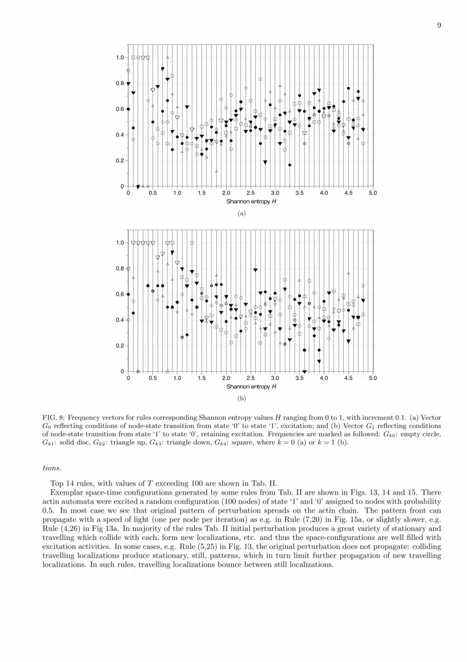
The frequency vectors as a function of Shannon entropy are shown in Fig. 8. Let us exemplify the construction. InFig. 8a for H = 0.9 we see labels in the following order: empty square, empty triangle up, empty circle, solid triangledown and solid disk. This means that rule-vector F0 corresponding to the rule generating configuration with entropyH = 0.9 more often has 1 in position 4, F04 = 1, less often in position 2, less often in position 0, less often in position3 and less often in position 1. In words, if a rule generates space-time configurations with entropy H = 0.9 then morelike a resting is excited if it has four neighbours, less like two neighbours, less likely zero neighbours, less likely threeneighbours and almost never one neighbour. To detect what number of neighbours exciting a node is most responsiblefor generating configurations of certain entropy we select, for each class/interval of entropy, only positions which havemaximum frequencies in the class/interval. Thus for a transition from state ‘0’ to state ‘1’ the following numbers ofexcited neighbours are most critical, they are ordered in increase of H: 444443324234 344000000110 4402222222411433141211. The corresponding sequence for a transition from state ‘1’ to state ‘1’ is 444444444434 400121330034331110401244 0003442420. The sequences are intentionally split into four parts each, the parts corresponds to fourequal intervals of the entropy H. For each interval we calculate dominating position as follows. For 0 ≤ H ≤ 1.25transitions 0→ 1 and 1→ 1 happen more likely if four neighbours are excited. For entropy in the interval ]1.25, 2.5]node excites or remains excited even if no neighbours are excited, autonomous excitation. Autonomous excitationspose little interest in term communication of signals via travelling localizations, therefore we discard dominatingposition 0 and look at the sub-sequences 344000000110 (transition 0 → 1) and 400121330034 (transition 1 → 1).We see that dominating positions for transition 0 → 1 are 1 and 4, and for transition 1 → 1 dominating positionis 3. When entropy exceeds 2.5 and yet remains below 3.75 a resting cell excites more likely when it has 2 excitedneighbours and remains excited if it has 1 excited neighbour. For the highest values of entropy, 3.75 < H ≤ 5 weobserve dominating number of neighbours 1 for transition 0→ 1 and 0 for 1→ 1.

Proposition 1 Shannon entropy of space-time configurations generated by actin automata is proportional to sensi-tivity of actin chain nodes: the higher is sensitivity the larger values of entropy the configurations have.

6

Sim

pson

div

ersi

ty in

dex

D

0

0.2

0.4

0.6

0.8

1.0

Shannon entropy H0 0.5 1.0 1.5 2.0 2.5 3.0 3.5 4.0 4.5 5.0 5.5

(a)

(b) (c)

(d) (e)

(f) (g)

FIG. 6: Shannon entropy versus Simpson diversity index. (a) Plot H vs. D. (b–g) Space-time configurations developed ofautomaton x chain governed by exemplar rules: (b) Rule (10,10), H(10, 10) = 4.8, (c) Rule (11,6), H(11, 6) = 4.5, (d) Rule(7,29), H(7, 29) = 4, (e) Rule (11,14), H(11, 14) = 3.5, (f) Rule (14,9), H(14, 9) = 3, (g) Rule (20,13), H(20, 13) = 2.5. Timegoes down. A node in state ‘1’ is black pixel, and in state ‘0’ is blank. Initially the automata are perturbed by a randomconfiguration of 100 nodes, where each takes ‘0’ or ‘1’ with probability 0.5.

7

Num

ber o

f rul

es

0

10

20

30

40

Shannon entropy H0 0.5 1.0 1.5 2.0 2.5 3.0 3.5 4.0 4.5 5.0

FIG. 7: Distribution of a number of rules on Shannon entropy H values of the space-time configurations. The line is anapproximation of the distribution by a polynomial of degree five.

With increase of entropy dominating number of neighbours necessary to excite a resting node or to keep excitednode excited is decreasing as 4 to 1, 4 to 2 to 1 and 4 to 3 to 1 to 0. This is a reflection of increased sensitivity ofactin nodes. Decrease of local excitation necessary to keep a node excited (4→ 3→ 1→ 0 can be also interpreted asincrease in sustainability of excitation, or even as a transition from lateral excitation to lateral inhibition. Namely, forentropy in the interval H ∈ [0, 1.25] an excited node stays excited if it has four excited neighbours and H ∈]1.25, 2.5]if it has three excited neighbours. That is excited nodes in actin automata stimulate each other and thus stay excitedlonger. The situation is changed from lateral stimulation to rather lateral inhibition when entropy exceeds 2.5: anexcited node remains excited if one neighbour, H ∈]2.5, 3.75], or no neighbours, H ∈]3.75, 5], are excited; this can beinterpreted as that an excessive amount of excited neighbours inhibits excitation of a node.

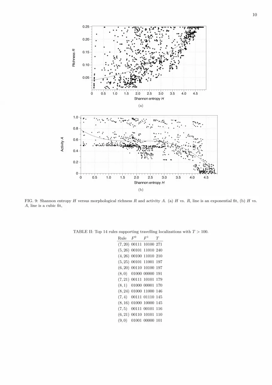
We could expect that morphological richness R, ratios of different 3× 3 patterns in space-time configurations willbe proportional to entropy H. As we can see in Fig. 9a, this is indeed the case. Richness R grows exponentially withincrease of the entropy. Activity A is not a good indicator of morphological complexity the automata dynamics, aswe can see in Fig. 9b, activity remains rather stable for the entropy below 3.5 and only starts to substantially dropdown when H exceed 4. This is because A depends a ratio of excited nodes and truly complex structures have ratherlow level of excitations yet elaborately arranged interacting patterns of the excitation.

There is a poor correlation between Shannon entropy H and incoherence I (Fig. 10a). The incoherence indicateshow strongly are two chains of actin polymers are desynchronised and might reflect that there are different typesof patterns propagating almost independently on the parallel chains of actin units. With regards to compressibilityZ, the relation could be approximated by quadratic polynomial, where rules with H between 2 and 2 has lowestindicators of compressibility (Fig. 10b).

IV. LOCALIZATIONS

Distribution of rules on a number of seeds supporting localizations (Fig. 11) is quite uniform, there are rules whichdevelop fifty seeds into localizations and there are rules where almost every seeds leads to a stationary or propagatinglocalisation. 705 of 1024 rules, e.g. almost 69%, do not support any localizations, neither stationary nor travelling.By arranging rules in the descending order on a number of seeds they develop into localisation we can consider threeimportant cases: rules that support traveling localizations, rules that support stationary, rules that support bothstationary and mobile localisation.

A. Travelling localisations

Rules supporting travelling localizations and the integral characteristics of the rules are shown in Tab. I. A plot ofentropy H versus T (Fig. 12) shows that rules with lowest values of the localizations richness T show high dispersionin H, they exhibit oscillations in entropy, with amplitude circa 1.5. The rules with T exceeding 40, i.e. those whichdevelop 40 seeds into the localizatios, show entropy values around 4.

Proposition 2 Higher values of Shannon entropy are typical for rules supporting large number of travelling localiza-

8

TABLE I: Rules supporting travelling localizations.Rule T H D R P A I Z

(7, 20) 271 4.31 0.98 0.22 0.84 0.32 0.28 6.67E-006

(5, 26) 240 4.70 0.99 0.25 0.92 0.39 0.39 6.40E-006

(4, 26) 210 4.54 0.99 0.25 0.86 0.31 0.34 6.92E-006

(5, 25) 197 3.83 0.95 0.25 0.73 0.14 0.19 1.37E-005

(6, 20) 197 4.37 0.98 0.25 0.86 0.37 0.28 6.33E-006

(8, 0) 191 3.50 0.96 0.08 0.83 0.23 0.26 6.82E-006

(7, 21) 179 4.31 0.98 0.22 0.97 0.56 0.39 5.97E-006

(8, 1) 170 3.50 0.96 0.09 0.84 0.23 0.26 6.81E-006

(8, 24) 146 3.71 0.97 0.19 0.80 0.25 0.18 7.39E-006

(7, 4) 145 2.75 0.92 0.20 0.54 0.06 0.07 1.82E-004

(8, 16) 145 3.54 0.96 0.13 0.77 0.24 0.17 7.61E-006

(7, 5) 116 4.31 0.98 0.21 0.93 0.29 0.24 8.71E-006

(6, 21) 110 4.40 0.98 0.25 0.70 0.14 0.14 1.28E-005

(9, 0) 101 3.69 0.97 0.09 0.92 0.30 0.36 6.17E-006

(9, 1) 85 3.70 0.97 0.09 0.91 0.30 0.36 6.15E-006

(9, 16) 85 3.63 0.96 0.14 0.81 0.26 0.18 7.18E-006

(10, 16) 78 3.96 0.98 0.16 0.90 0.32 0.29 6.19E-006

(10, 24) 77 4.20 0.98 0.23 0.92 0.34 0.29 6.14E-006

(10, 0) 72 3.69 0.97 0.09 0.93 0.30 0.39 6.15E-006

(8, 2) 64 4.02 0.98 0.18 0.90 0.29 0.32 6.19E-006

(8, 3) 63 4.03 0.98 0.18 0.90 0.29 0.32 6.18E-006

(10, 1) 58 3.69 0.97 0.09 0.92 0.30 0.40 6.14E-006

(9, 24) 57 3.79 0.97 0.21 0.82 0.27 0.20 7.21E-006

(5, 6) 52 4.20 0.98 0.25 0.88 0.46 0.20 6.43E-006

(6, 26) 44 4.67 0.99 0.25 0.96 0.49 0.45 6.19E-006

(5, 24) 38 2.57 0.83 0.22 0.54 0.08 0.14 5.61E-005

(8, 17) 38 4.25 0.98 0.18 0.91 0.33 0.26 6.17E-006

(4, 28) 37 2.83 0.86 0.19 0.94 0.50 0.39 2.35E-005

(5, 28) 36 4.24 0.98 0.23 0.91 0.41 0.34 6.11E-006

(8, 8) 36 4.26 0.98 0.20 0.93 0.32 0.39 6.26E-006

(5, 21) 32 3.31 0.92 0.25 0.36 0.06 0.08 1.08E-005

(8, 9) 32 4.31 0.98 0.21 0.93 0.33 0.40 6.17E-006

(9, 2) 32 4.11 0.98 0.19 0.94 0.31 0.36 6.05E-006

(9, 3) 32 4.13 0.98 0.19 0.94 0.32 0.36 6.02E-006

(10, 17) 31 4.38 0.99 0.21 0.95 0.37 0.36 5.91E-006

(10, 25) 29 4.57 0.99 0.25 0.94 0.39 0.35 5.90E-006

(6, 10) 28 4.62 0.99 0.25 0.90 0.46 0.45 6.36E-006

(8, 25) 27 4.28 0.98 0.22 0.91 0.33 0.28 6.25E-006

(10, 2) 27 4.19 0.98 0.23 0.95 0.34 0.42 5.92E-006

(10, 3) 27 4.28 0.98 0.22 0.95 0.36 0.41 5.90E-006

(6, 24) 25 3.35 0.92 0.21 0.84 0.16 0.25 2.00E-005

(4, 27) 22 4.20 0.97 0.25 0.88 0.27 0.23 1.02E-005

(6, 11) 22 1.07 0.39 0.24 0.98 0.84 0.04 1.54E-004

(7, 24) 22 3.96 0.97 0.19 0.93 0.43 0.71 1.27E-005

(4, 6) 21 2.18 0.85 0.23 0.97 0.60 0.58 1.21E-004

(6, 5) 20 3.60 0.95 0.25 0.47 0.07 0.08 1.51E-004

(10, 8) 20 4.48 0.99 0.23 0.95 0.37 0.39 5.90E-006

(11, 16) 19 4.03 0.98 0.16 0.95 0.36 0.34 5.98E-006

(10, 9) 18 4.61 0.99 0.25 0.96 0.39 0.41 5.84E-006

(11, 24) 17 4.27 0.98 0.23 0.96 0.40 0.35 6.00E-006

(6, 4) 16 2.55 0.90 0.23 0.44 0.05 0.04 4.65E-004

(6, 25) 15 3.25 0.94 0.23 0.98 0.61 0.33 1.03E-005

(8, 21) 15 4.53 0.99 0.23 0.95 0.39 0.41 5.87E-006

(4, 21) 13 3.05 0.87 0.25 0.39 0.03 0.06 1.83E-004

(5, 20) 13 2.74 0.85 0.25 0.39 0.03 0.06 1.87E-004

(5, 11) 11 1.81 0.55 0.25 0.45 0.19 0.04 3.46E-004

(7, 10) 11 4.35 0.98 0.22 0.94 0.50 0.46 6.47E-006

(4, 25) 10 3.34 0.91 0.23 0.60 0.10 0.14 1.98E-005

(9, 21) 10 4.57 0.99 0.25 0.96 0.40 0.42 5.83E-006

(4, 20) 8 2.57 0.84 0.25 0.38 0.03 0.06 2.71E-006

(7, 8) 8 1.84 0.69 0.17 0.92 0.42 0.83 1.71E-006

(5, 10) 6 4.41 0.98 0.25 0.09 0.00 0.00 2.68E-004

(8, 10) 6 4.48 0.98 0.23 0.96 0.37 0.45 5.92E-006

(8, 11) 6 4.43 0.98 0.23 0.96 0.39 0.44 5.97E-006

(5, 27) 5 0.54 0.13 0.25 0.98 0.32 0.04 2.51E-004

(4, 22) 4 2.62 0.89 0.24 0.93 0.41 0.39 1.74E-004

(5, 4) 4 2.95 0.92 0.23 0.25 0.02 0.02 8.79E-004

(5, 5) 4 3.45 0.95 0.25 0.24 0.04 0.04 5.32E-004

(5, 14) 3 2.80 0.88 0.12 0.96 0.37 0.25 7.01E-005

(4, 10) 2 4.48 0.98 0.25 0.05 0.00 0.00 4.36E-004

(7, 9) 2 4.19 0.98 0.22 0.95 0.48 0.58 8.30E-006

(7, 11) 2 0.78 0.25 0.15 0.98 0.85 0.01 1.99E-006

(7, 19) 1 2.93 0.90 0.15 0.93 0.48 0.17 1.40E-004

(8, 20) 1 4.42 0.98 0.23 0.95 0.37 0.37 5.99E-006

(12, 0) 1 2.85 0.92 0.08 0.84 0.24 0.10 1.45E-005

(12, 1) 1 2.85 0.92 0.08 0.84 0.24 0.27 1.25E-005

(12, 16) 1 2.85 0.92 0.09 0.84 0.24 0.13 1.45E-005

9

0

0.2

0.4

0.6

0.8

1.0

Shannon entropy H0 0.5 1.0 1.5 2.0 2.5 3.0 3.5 4.0 4.5 5.0

(a)

0

0.2

0.4

0.6

0.8

1.0

Shannon entropy H0 0.5 1.0 1.5 2.0 2.5 3.0 3.5 4.0 4.5 5.0

(b)

FIG. 8: Frequency vectors for rules corresponding Shannon entropy values H ranging from 0 to 1, with increment 0.1. (a) VectorG0 reflecting conditions of node-state transition from state ‘0’ to state ‘1’, excitation; and (b) Vector G1 reflecting conditionsof node-state transition from state ‘1’ to state ‘0’, retaining excitation. Frequencies are marked as followed: Gk0: empty circle,Gk1: solid disc, Gk2: triangle up, Gk3: triangle down, Gk4: square, where k = 0 (a) or k = 1 (b).

tions.

Top 14 rules, with values of T exceeding 100 are shown in Tab. II.Exemplar space-time configurations generated by some rules from Tab. II are shown in Figs. 13, 14 and 15. There

actin automata were excited a random configuration (100 nodes) of state ‘1’ and ‘0’ assigned to nodes with probability0.5. In most case we see that original pattern of perturbation spreads on the actin chain. The pattern front canpropagate with a speed of light (one per node per iteration) as e.g. in Rule (7,20) in Fig. 15a, or slightly slower, e.g.Rule (4,26) in Fig 13a. In majority of the rules Tab. II initial perturbation produces a great variety of stationary andtravelling which collide with each, form new localizations, etc. and thus the space-configurations are well filled withexcitation activities. In some cases, e.g. Rule (5,25) in Fig. 13, the original perturbation does not propagate: collidingtravelling localizations produce stationary, still, patterns, which in turn limit further propagation of new travellinglocalizations. In such rules, travelling localizations bounce between still localizations.

10

RIc

hnes

s R

0.05

0.10

0.15

0.20

0.25

Shannon entropy H0 0.5 1.0 1.5 2.0 2.5 3.0 3.5 4.0 4.5

(a)

Activ

ity A

0

0.2

0.4

0.6

0.8

1.0

Shannon entropy H0 0.5 1.0 1.5 2.0 2.5 3.0 3.5 4.0 4.5

(b)

FIG. 9: Shannon entropy H versus morphological richness R and activity A. (a) H vs. R, line is an exponential fit, (b) H vs.A, line is a cubic fit,

TABLE II: Top 14 rules supporting travelling localizations with T > 100.

Rule F 0 F 1 T

(7, 20) 00111 10100 271

(5, 26) 00101 11010 240

(4, 26) 00100 11010 210

(5, 25) 00101 11001 197

(6, 20) 00110 10100 197

(8, 0) 01000 00000 191

(7, 21) 00111 10101 179

(8, 1) 01000 00001 170

(8, 24) 01000 11000 146

(7, 4) 00111 01110 145

(8, 16) 01000 10000 145

(7, 5) 00111 00101 116

(6, 21) 00110 10101 110

(9, 0) 01001 00000 101

11

Inco

here

nce I

0

0.0005

0.0010

0.0015

Shannon entropy H0 0.5 1.0 1.5 2.0 2.5 3.0 3.5 4.0 4.5 5.0

(a)

Com

pres

sibi

lity Z

0

0.0005

0.0010

0.0015

Shannon entropy H0 0.5 1.0 1.5 2.0 2.5 3.0 3.5 4.0 4.5 5.0

(b)

FIG. 10: The entropy versus incoherence and compressibility. (a) H vs. I, .(b) H vs. Z.

Num

ber o

f fun

ctio

ns

0

5

10

15

20

Number of seeds100 200 300 400 500 600 700 800 900 1000

FIG. 11: Distribution of a number of rules supporting localizations on a number of seeds which leads to the localizations.

12

Shan

non

entro

py H

0

1

2

3

4

5

Travelling localisations richness T0 20 40 60 80 100 120 140 160 180 200 220 240 260

FIG. 12: Travelling localizations richness T versus Shannon entropy H

(a) (b)

FIG. 13: Exemplar space-time configurations generated by (a) Rule (4,26) and (b) Rule (5,25).

13

(a) (b)

FIG. 14: Exemplar space-time configurations generated by (a) Rule (5,26) and (b) Rule (6,20).

Let us calculate frequency vectors V 0 and V 1 from F 0 and F 1. There are fourteen rules in Tab. II, V 0i is a ratio of ‘1’

in F 0i to 7, the same for V1. Thus we have V 0 = (0 5

14914

64

714 ) and V 1 = ( 9

14514

614

314

514 ). Probabilities of excitation can

be represented via a polynomial approximation of vectors V 0 and V 1 shown in Fig. 16a, compare with the probabilityof excitation of the rules not supporting any localizations in Fig. 16b.

Assuming 0.5 is a cut off frequency, we can transform the vector to a simplified form: ∗V 0 = (00101) and ∗V 1 =(10000).

Proposition 3 A rule more likely supports large number of traveling localizations if it has the following node statetransitions. A resting node becomes excited if it has two or four excited neighbours. An excited node remains excitedif it has no excited neighbours.

B. Stationary localisations

Let us calculate frequency vectors V 0 and V 1 from F 0 and F 1 for rules supporting stationary localizations. Thereare 39 rules that exhibit stationary localizations for over 900 (of 1024) seeds. V 0

i is a ratio of ’1’ in F 0i to 39, the

14

(a) (b)

FIG. 15: Exemplar space-time configurations generated by (a) Rule (7,20) and (b) Rule (7,21).

same for V1. Thus we have V 0 = (00 1539

2039

1939 ) and V 1 = ( 27

392739

3039

2139

1939 ). Probabilities of excitation can be represented

via a polynomial approximation of vectors V 0 and V 1 shown in Fig. 17a, compare with the probability of excitationof the rules that support travelling localizations in Fig. 16b and rules that do not support any localizations inFig. 16b. Assuming 0.5 is a cut off frequency, we can transform the vectors to a simplified form: ∗V 0 = (00010) and∗V 1 = (11110).

Proposition 4 A rule more likely supports large number of stationary localizations if it has the following node statetransitions. A resting node becomes excited only if three of its four neighbours are excited. An excited node remainsexcited if it has less four excited neighbours.

C. On rules supporting both stationary and travelling localisaitons

Scatter of a number T of seeds supporting travelling localizations in each rule R vs number T of seeds supportingstationary localizations in the same rule R is shown in Fig. 18. The plot shows that typically the more travelling

15

Prob

abilit

y of

exc

itatio

n

0

0.2

0.4

0.6

Neighbourhood occupancy0 0.5 1.0 1.5 2.0 2.5 3.0 3.5 4.0 4.5

(a)

Prob

abilit

y of

exc

itatio

n

0

0.2

0.4

0.6

0.8

1.0

Neighbourhood occupancy0 0.5 1.0 1.5 2.0 2.5 3.0 3.5 4.0 4.5

(b)

FIG. 16: Dependence of a probability of excitation of a node in actin automaton (a) supporting travelling localizations and(b) not supporting any localizations (neither stationary nor travelling) on a number of excited neighbours of the node. Thepolynomial of the probability (a) is calculated on 14 rules that exhibit travelling localizations for largest number of seeds, andthe polynomial of the probability (b) is calculated on 705 rules not supporting any localizations. Dashed line shows probabilityof excitation of a resting node, solid line of an excited node, i.e. of an excited node to remain excited.

Prob

abilit

y of

exc

itatio

n

0

0.5

1.0

Neighbourhood occupancy0 0.5 1.0 1.5 2.0 2.5 3.0 3.5 4.0 4.5

FIG. 17: Dependence of a probability of excitation of a node in actin automaton supporting stationary localizations on anumber of excited neighbours of the node. The polynomial of the probability is calculated on 39 rules that exhibit stationarylocalizations for 900 seeds. Dashed line shows probability of excitation of a resting node, solid line of an excited node, i.e. ofan excited node to remain excited.

Stat

iona

ry S

0

200

400

600

800

1000

Travelling T0 50 100 150 200 250 300

FIG. 18: Scatter of a number T of seeds supporting travelling localizations in each rule R vs number T of seeds supportingstationary localizations in the same rule R

16

TABLE III: Rules developing a maximum number of seeds into travelling and stationary localizations.

Rule F 0 F 1 T S H D R P A I Z

(4,26) 00100 11010 210 731 4.54 0.98 0.25 0.86 0.31 0.34 6.9E-6

(5,25) 00101 11001 197 724 3.83 0.95 0.25 0.73 0.14 0.19 1.3E-5

(7,4) 00111 00100 145 791 2.75 0.92 0.19 0.54 0.06 0.07 1.8E-4

(5,26) 00101 11010 240 388 4.70 0.99 0.25 0.92 0.39 0.39 6.4E-6

(6,21) 00110 10101 110 694 4.40 0.98 0.25 0.70 0.14 0.14 1.3E-5

(7,5) 00111 00101 116 682 4.31 0.98 0.21 0.93 0.29 0.24 8.7E-6

(7,21) 00111 10101 179 358 4.31 0.98 0.22 0.97 0.56 0.39 6E-6

localizations a rule exhibit the less stationary localizations the rule shows. There are however rules which show highnumber of seeds leading to travelling and seeds leading to stationary localizations. They are shown in Tab. III.

Configurations generated by rules in Tab. III from selected seeds are shown in Fig. 19. Rules (4,26) and (5,25)show a rich dynamics of traveling localizations (Fig. 19a–g). For most seeds the developments leads to formation ofseveral propagating localizations, some of them could be classed as glider guns, often travelling localizations producestationary localizations during their interactions with each other, e.g. Fig. 19be. In some cases, e.g. Fig. 19cfg wecan observe very elaborate trajectories of travelling licalisaitons.

In rule (7,4) a seed typically leads to formation of a single glider (Fig. 19h) or a pair of gliders moving in oppositedirections (Fig. 19i); some seeds can produce a glider and a stationary localisation (Fig. 19j). Rule (7,5) exhibitscombinations of travelling localizations and breathers: periodically oscillating stationary localizations (Fig. 19kl).

A good variety of travelling and stationary localizations is given in space-time dynamics of rule (7,21). Theseinclude large gliders propagating with a speed less than sped of light (‘speed of light’ glider translate one node periteration) (Fig. 19m), very slowly propagating localizations, or complex clusters of gliders, emitting stationary andtravelling localisaitons (Fig. 19n), combinations of large still lifes and gliders (Fig. 19p) and generation of two glidersof different sizes from a single seed (Fig. 19q).

What is important for a rule to be supportive for both travelling and stationary localizations?Let us calculate frequency vectors V 0 and V 1 from F 0 and F 1. There are seven rules in Tab. III, V 0

i is a ratio of‘1’ in F 0

i to 7, the same for V1. Thus we have V 0 = (001 4757 ) and V 1 = ( 5

737472747 ). Probabilities of excitation can

be represented via a polynomial approximation of vectors V 0 and V 1 shown in Fig. 20. Assuming 0.5 is a cut offfrequency, we can transform the vector to a simplified form: ∗V 0 = (00111) and ∗V 1 = (10101).

Proposition 5 An actin automaton supports highest number of travelling and stationary localizations if its localactivity is governed as follows. A resting node excites if it necessarily has two excited neighbours or likely three ormore likely five excited neighbours. An excited node remains excited if it has no excited neighbours or two or fourexcited neighbours.

Thus rule (7, 4) is most representative in terms F0 and rule (6, 12) is most representative in terms of F1.What integral characteristics are typical for the above localisation supporting rules?The Shannon entropy H is over 4 for most rules in Tab. III but rule (7, 4). Simpson diversity index D is over

0.9. Thus the rules which support both stationary and travelling localizations show very rich space time dynamics ofexcitations, R, when perturbed with a random initial pattern. They also show a moderate degree of space filling D,where, in case of random stimulation, the dynamical excitation fills over 50% of the automaton chains. Rule (7,21) isa highest space filler, with almost 97% of nodes being excited and rule (7,4) is a lowest space filler with just a half ofnodes typically occupied by excitation during the automaton development.

The space-time configurations are not overly rich morphologically with only circa 25% of possible local configu-rations presented. Activity levels vary substantially between the rules in Tab. III. Rule (7,4) shows lowest level ofoverall excitation activity followed by rules (5, 25) and (6,21). Highest level of activity are observed in space-timeconfigurations of rule (7,21). Rules (7,4), (5,21) and (6,21) show highest compressibility Z, which is due to lowerrichness R and, partly, space filling P .

Proposition 6 Rules supporting both travelling and stationary localizations are characterised by high Shannon entropyand Simpson diversity, low levels of activity, and high degree of compressibility.

Can we detect rules supporting localizations from integral characteristics of the space-time configurations generatedby the rules? Let us look at the Tab. IV. We see that space filling P is not a reliable discriminator but Shannon entropyH, activity level A and incoherence I are good discriminators on absence/presence and mobility of localizations.

17

(a) (b) (c)

(d) (e) (f)

(g) (h) (i)

(j) (k) (l)

(m) (n) (o)

(p) (q)

FIG. 19: Exemplar configuration of rules from Tab. III. In each subfigure space-time states of chain x, left, and y, right, areshown. (a) Rule (4, 26), seeds 01100 and 10001, (b) Rule (5, 25), seeds 00100 and 00011, (c) Rule (5, 25), seeds 00101 and00011, (d) Rule (5, 25), seeds 00101 and 01101, (e) Rule (5, 25), seeds 00110 and 00001, (f) Rule (5, 25), seeds 10001 and10111, (g) Rule (5, 25), seeds 11010 and 10011, (h) Rule (7, 4), seeds 00001 and 00111, (i) Rule (7, 4), seeds 00001 and 01111,(j) Rule (7, 4), seeds 00001 and 11100, (k) Rule (7, 5), seeds 00101 and 00111, (l) Rule (7, 5), seeds 00111 and 00100, (m) Rule(7, 21), seeds 00011 and 10110, (n) Rule (7, 21), seeds 00011 and 11111, (o) Rule (7, 21), seeds 00100 and 10001, (p) Rule (7,21), seeds 01001 and 01000, (r) Rule (7, 21), seeds 10110 and 11100.

Proposition 7 Actin automata rules supporting highest number travelling localizations show high Shannon entropyH, medium activity A and high incoherence I. The rules supporting highest number of stationary localizations showlow entropy H, low activity A and low incoherence I.

V. DISCUSSION

In an exhaustive computational analysis of automaton models of hypothetical actin fibre communication events, wehave discovered how to pinpoint rules supporting travelling and stationary localizations from global characteristicsof space-time configurations generated by the actin automata rules. Nearly one third of node-state transition rulessupport either stationary or travelling localizations. Most the rules supporting localizations are ‘specialized’: theysupport either stationary localizations or travelling localizations. Around 3% of the rules shows rich dynamics ofboth travelling and stationary localizations, these rules are rare finds in the space of actin automaton node-state

18

Prob

abilit

y of

exc

itatio

n

−0.5

0

0.5

1.0

Neighbourhood occupancy0 0.5 1.0 1.5 2.0 2.5 3.0 3.5 4.0 4.5

FIG. 20: Dependence of a probability of excitation of a node in actin automaton supporting stationary and travelling local-izations n a number of excited neighbours of the node. The polynomial of the probability is calculated on 7 rules that exhibitstationary and travelling localizations for largest number of seeds. Dashed line shows probability of excitation of a resting node,solid line of an excited node, i.e. of an excited node to remain excited.

TABLE IV: Statistical characterisation of main groups of rules. For each characteristics the table shows average and standarddeviation

H, σ D, σ R, σ P , σ A, σ I, σ

All rules 2.8, 1.2 0.8, 0.2 0.1, 0.1 0.9, 0.2 0.5, 0.2 0.2, 0.2

Rules supporting travelling localizations 3.6, 0.9 0.9, 0.1 0.2, 0.0 0.8, 02 0.3, 0.2 0.3, 0.2

Rules supporting stationary localizations 2.3, 0.6 0.8, 0.1 0.1, 0.1 0.7, 0.2 0.1, 0.1 0.1, 0.0

Rules supporting travelling and stationary localizations 4.1, 0.7 1.0, 0.0 0.2, 0.0 0.8, 0.2 0.3, 0.2 0.2, 0.1

Rules supporting no localizations 2.9, 1.3 0.8, 0.2 0.2, 0.1 0.9, 0.1 0.6, 0.2 0.3, 0.2

transitions. Rules supporting large numbers of travelling localizations usually produce space-time configurations withhigh Shannon entropy values, i.e. a higher potential information content. Rules which support both travelling andstationary localizations generate configurations with high Shannon entropy and Simpson diversity index yet showinglow levels of excitation activity and high degrees of compressibility. The rules supporting only stationary localizationsexhibit low levels of excitation activity, low incoherence and low Shannon entropy.

The above findings are valuable yet not efficient when searching for localizations in chains of biopolymers such asactin. It would seem to be more practical to decide on whether a rule supports localisation incidence by analysingthe structure of the rule; we have proposed how this can be done.

We also found that a rule supports travelling localizations if a resting node excites if it has two or four excitedneighbours (50% or 100% of neighbourhood excitation) and an excited node remains excited if it has no excited neigh-bours. Indeed, additional modes of excitability might be necessary to support propagation of the localisation. A rulesupports stationary localizations if a resting node excites if it has three excited neighbours (c. 70% of neighbourhoodis excited) and an excited node remains excited if it has less than four excited neighbours.

But how can these models be applied to the proposed biophysical model of actin-based cellular communications?Whilst analysis of automaton patterns is inherently subjective [12], rules which support travelling localizations ar-guably form random patterns, whereas the few rules which support travelling and stationary localizations tend toappear more oscillatory. The observation the former, which may be described as emergent (i.e. apparent complexityarising from simple inputs and rules), provides a theoretical basis for describing the evolution and dynamics of complexpatterns in biological systems. For example, if the actin cytoskeleton is considered as a sensorimotor data network,as we are suggesting, it may reasonably be hypothesised that emergent data patterns therein are a viable origin forthe evolution of diverse, complex behaviours, even in unicellular organisms: such behaviours may be interpreted asintelligence, or at least efficient adaptations to cellular computation which favour survival. This finding substantiatesour hypotheses in a previous paper [16], in which we attempt to explain how apparently ‘intelligent’ behaviour inuni/acellular organisms such as protists may be generated in a cytoskeletal cellular communications system.

Our further studies will concern with developing working computing circuits on actin filament networks whichtopologies are closely matching topologies of the real intracellular networks.

[1] Andrew Adamatzky. Collision-based computing in biopolymers and their automata models. International Journal ofModern Physics C, 11(07):1321–1346, 2000.

19

[2] Andrew Adamatzky. In Andrew Adamatzky, editor, Collision-based Computing, chapter New Media for Collision-basedComputing, pages 411–442. Springer-Verlag, London, UK, UK, 2002.

[3] Andrew Adamatzky. Topics in reaction-diffusion computers. Journal of Computational and Theoretical Nanoscience,8(3):295–303, 2011.

[4] Andrew Adamatzky. On diversity of configurations generated by excitable cellular automata with dynamical excitationintervals. International Journal of Modern Physics C, 23(12), 2012.

[5] Andrew Adamatzky. Patterns of conductivity in excitable automata with updatable intervals of excitations. PhysicalReview E, 86(5):056105, 2012.

[6] Andrew Adamatzky and Leon O Chua. Phenomenology of retained refractoriness: On semi-memristive discrete media.International Journal of Bifurcation and Chaos, 22(11), 2012.

[7] Andrew I Adamatzky. Universal computation in excitable media: the 2+ medium. Advanced materials for optics andelectronics, 7(5):263–272, 1997.

[8] L Belmont, A Orlova, D Drubin, and E Egelman. A change in actin conformation associated with filament instability afterpi release. PNAS, 96(1):29–34, 1999.

[9] R Dominguez and K Holmes. Actin structure and function. Annual Review of Biophysics, 40:169–86, 2011.[10] S Hameroff. Quantum computation in brain microtubules? the penrose—hameroff ‘orch or’ model of consciousness.

Philosophical Transactions of the Royal Society of London A, 356(1743):1869–1896, 1998.[11] Y Hwang and A Barakat. Dynamics of mechanical signal transmission through prestressed stress fibres. PLoS One,

7(4):e35343, 2012.[12] Navot Israeli and Nigel Goldenfeld. Coarse-graining of cellular automata, emergence, and the predictability of complex

systems. Phys. Rev. E, 73:026203, Feb 2006.[13] P Janmey. The cytoskeleton and cell signalling: component localization and mechanical coupling. Physiological Reviews,

78(3):763–781, 1998.[14] M Jibu, S Hagan, S Hameroff, K Pribram, and K Yasue. Quantum optical coherence in cytoskeletal microtubules:

implications for brain function. Biosystems, 32(3):195–209, 1994.[15] R Lahoz-Beltra, S Hameroff, and J Dayhoff. Cytoskeletal logic: a model for molecular computation via boolean operations

in microtubules and microtubule-associated proteins. Biosystems, 29(1):1–23, 1993.[16] R Mayne, J Jones, and A Adamatzky. On the role of the plasmodial cytoskeleton infacilitating intelligent behaviour in the

slime mould physarum polycephalum. In press, 2014.[17] M Mofrad and R Kamm. Cytoskeletal mechanics: models and measurements in cell mechanics. Cambridge University

Press, Cambridge, first edition, 2006.[18] Shigeru Ninagawa and Andrew Adamatzky. Classifying elementary cellular automata using compressibility, diversity and

sensitivity measures. International Journal of Modern Physics C, 25(03), 2014.[19] Toshiro Oda, Mitsusada Iwasa, Tomoki Aihara, Yuichiro Maeda, and Akihiro Narita. The nature of the globular-to

fibrous-actin transition. Nature, 457(7228):441–445, 2009.[20] V Petit and JP Thiery. Focal adhesions: structure and dynamics. Biology of the Cell, 92:477–494, 2000.[21] Markus Redeker, Andrew Adamatzky, and Genaro J Martınez. Expressiveness of elementary cellular automata. Interna-

tional Journal of Modern Physics C, 24(03), 2013.[22] J Southgate, P Harnden, and L Trejdosiewicz. Cytokeratin expression patterns in normal and malignant urothelium: a

review of the biological and diagnostic implications. Histology and Histopathology, 14(2):657–664, 1999.[23] Rita Toth, Christopher Stone, Ben de Lacy Costello, Andrew Adamatzky, and Larry Bull. Simple collision-based chemical

logic gates with adaptive computing. International Journal of Nanotechnology and Molecular Computation (IJNMC),1(3):1–16, 2009.

[24] J Tuszynski, S Portet, J Dixon, C Luxford, and H Cantiello. Ionic wave propagation along actin filaments. BiophysicalJournal, 86:1890–1903, 2004.

[25] S Winder and K Ayscough. Cell science at a glance: Actin-binding proteins. Journal of Cell Science, 118:651–654, 2005.[26] Liang Zhang and Andrew Adamatzky. Collision-based implementation of a two-bit adder in excitable cellular automaton.

Chaos, Solitons & Fractals, 41(3):1191–1200, 2009.