Embed Size (px)
Citation preview
1
ACTUATORS AND SENSORS IN STRUCTURAL DYNAMICS
W. GAWRONSKI Jet Propulsion Laboratory California Institute of Technology Pasadena, CA 91 I09 [I. S. A.
1. Introduction
Flexible structure dynamics depend on the location and gains of actuator and sensors. This fact is often underestimated, although it is an important factor in the planning of structural dynamic tests, and in designing structural controllers. In this work we describe the impact of actuators and sensors gains and locations on structural Sroperties, which includes structural controllability and observability, and structural a x i modal norms. Using these properties we show how to detect a damage of structural members, how to place actuators and sensors for structural testing and control, and how to tune actuators or sensors to excite a selected mode or a set of selected modes. The reader can find background material in my book [ 5 ] . The analysis is conducted in modal state-space coordinates, which are described at the beginning of this paper.
2. Modal State-Space Representation
In this section both the standard and generalized state-space representations of a structure are discussed. Both representations are presented in modal coordinates.
2.1. STANDARD STATE-SPACE REPRESENTATION
Models of a linear time-invariant system are described in a standard form called state space representation, which is of the following form
X = Ax+Bu (1) y = c x
In the above equations the N-dimensional vector x is called the state vector, the s- dimensional vector u is the system input, and the r-dimensional vector y is the system output. The A, B, and C matrices are real constant matrices of approprihte dimensions (A is NxN, B is Nxs, and C is r x w .
A structural model, however, is typically represented by the well-known second-order model. Let n, be a number of degrees of fieedom of the system, let r be a number of
2
outputs, and let s be a number of inputs. A flexible structure in nodal coordinates is represented by the following equation:
Mq+ Dq+ Kq = B<,u
Y = coqq + C,,”9
In this equation q is the n, x 1 displacement vector; u is the s x 1 input vector, y is the output vector, r x 1 ; M is the mass matrix, n, x n, , D is the damping matrix, n, x n, , and K is the stiffness matrix, n, x nd . The input matrix Bo is n, x s , the displacement output matrix C, is r x n , , and the velocity output matrix C,, is r x n , . The mass matrix is positive definite, and the stifhess and damping matrices are positive semidefinite. On details of the derivation of these types of equations see [ 141, and [7].
The same equation can be represented in modal coordinates. Define the matrix of mode shapes (or modal matrix) Cg of dimensions n, x n , which consists of n natural modes of a structure
@=[4 42 ... 4”l
where 4j, i = 1, ..., n , is the ith modal vector. The modal matrix diagonalizes mass and stiffness matrices M and K, namely
The matrices M , and K,,, are diagonal. The matrix M , is called modal mass matrix, and K,,, is modal stiffness matrix.
The same transformation can be applied to the damping matrix
where Dm is the modal damping matrix. This matrix is not always obt;?ined diagonal. A damping matrix that can be diagonalized by the above transformation is called a matrix of proportional damping. For example, a linear combination of the stifhess and mass matrices, D = a,K + a,M , produces a proportional damping matrix, see [2], [7] (a, and a2 are non-negative scalars).
The second-order structural model (2) can be also expressed in modal coordinates by introducing a new variable, q, , called a modal displacement, such that
After some manipulations (see [SI) Eq.(2) is in the form
3
q, + 2ZRqm + R2qm = B,u
Y = Cmqqm +Cmvqm (7)
In the above equation R = diug(w,, w,, .... w,) is the matrix of natural frequencies, Z is the modal damping matrix, Z = diug(c, , c,,. .. ,<,) . where Ci is the damping of the ith
mode. The modal input matrix B, is obtained as
and in Eq.(7) we used the following modal displacement and rate matrices
Note that equation (7) is a set of uncoupled equations, since the matrices R and Z are diagonal. Thus, this set of equations can be re-written as follows
" i = 1 ..... n, where y = c y i , bmi is the ith row of B,,, . and cmqi . c,,. are the ith columns
i = l
of Cmq and C,, , respectively. In the above equations yi is the system output due to the zth mode dynamics. Note that the structural response y is a sum of modal responses y j , which is a key property used to derive structural properties in modal coordinates.
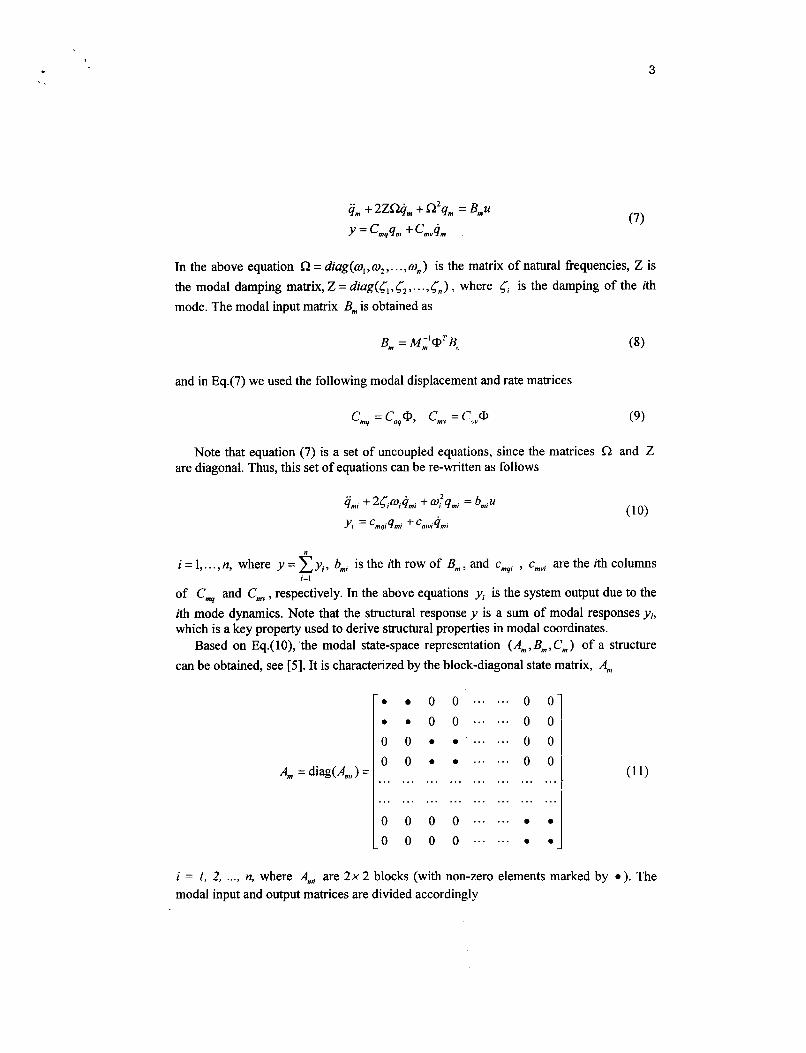
Based on Eq.( lo), 'the modal state-space representation (A,,,, B,, C,) of a structure can be obtained, see [ 5 ] . It is characterized by the block-diagonal state matrix, A,,,
4, = diag(&) =
. . . . . . . 0 0 0 0 0 0 0 0 0 0 0 0 . . . . . . . 0 0 0 0 0 . . . . . . . 0 0
. . . . . . .
. . . . . . . . . . . . . . . . . . . . . . . .
. . . . . . . . . . . . . . . . . . . . . . . . 0 0 0 0 . . . . . . 0 0
0 0 0 0 . . . . . . 0 0
i = I, 2, .... n, where Ai are 2x 2 blocks (with non-zero elements marked by 0 ) . The modal input and output matrices are divided accordingly
4
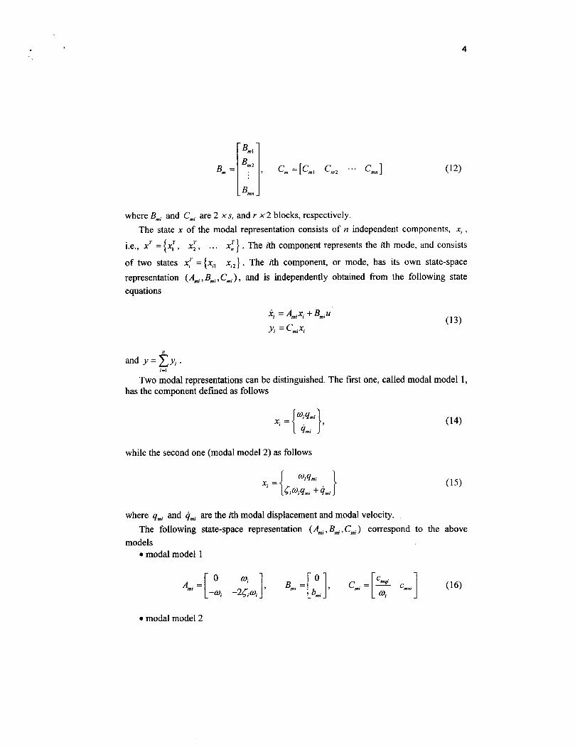
where B,, and C,; are 2 xs, and r x 2 blocks, respectively. The state x of the modal representation consists of n independent components, x, ,
i.e., x = {x, , x2, ... x:} . The ith component represents the ith mode, and consists
of two states x,T = {x,, x , ~ } . The ith component, or mode, has its own state-space representation (A,,,;, Bmi , Cmi) , and is independently obtained fiom the following state equations
T T T
xi = A,,,p; + Bmiu
y; = c,;xi (13)
Two modal representations can be distinguished. The first one, called modal model 1, has the component defined as follows
xi = { 7 }, while the second one (modal model 2) as follows
where qmi and qmi are the ith modal displacement and modal velocity.
models The following state-space representation (A,,,;, B,";, Cmj ) correspond to the above
0 modal model 1
0 modal model 2
5
2.2. GENERALIZED STATE-SPACE REPRESENTATION
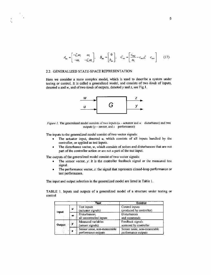
Here we consider a more complex model, which is used to describe a system under testing or control. It is called a generalized model, and consists of two kinds of inputs, denoted u and w, and of two kinds of outputs, denoted y and z, see Fig. 1.
W Z b
Figure 1. The generalized model consists of two inputs (u - actuator and w - disturbance) and two outputs 0, - sensor, and z - performance)
The inputs to the generalized model consist of two vector signals: 0
0
The actuator input, denoted u, which consists of all inputs handled by the controller, or applied as test inputs. The disturbance vector, w, which consists of noises and disturbances that are not part ofthe controller action or are not a part of the test input.
The sensor vector, y: it is the controller feedback signal or the measured test signal. The performance vector, z: the signal that represents closed-loop performance or test performance.
The outputs of the generalized model consist of two vector signals: 0
0
The input and output selection in the generalized model are listed in Table 1.
TABLE 1. Inputs and outputs of a generalized model of a structure under testing or control
6
Let A be the state matrix of the system, Bu and B, are the input matrices of u and w,
respectively, and Cy and C, are the output matrices of y and z, respectively; then the state space representation of the generalized model is as follows
X = Ax + B,u + B,w
Y = Cy%
z = C,Z
This model is transformed into the modal state-space representation the same way as the standard model previously described.
3. Controllability and Observability
System dynamics, excited at the input and measured at the output, are described by the state variables. However, the input may not be able to excite all states; consequently, it cannot fully control the system. Also, not all states may be represented at the output i.e., state dynamics may not be fully observed. Based on these two observations, we call a system controllable if the input excites all states and we call it observable if all the states are represented in the output
3.1. GRAMMIANS
We use grammians to evaluate the system controllability and observability properties. They are defined as follows (see, for example, [9], and [ 151)
m m
W, = jeA'BBTeAr'dz, W, = jeAr'CTCeA'dz 0 0
and are obtained fiom the Lyapunov equations:
A Wc + We A7' + BB" = 0, A" w, -t w, A + C7C = 0 (20)
For stable A, the obtained grammians W, and W, are positive definite. The eigenvalues of the grammians change during the coordinate transformation.
However, the eigenvalues of the grammian product are invariant. These invariants are denoted yi ,
where i = 1, . . . , N , and are called the Hankel singular values of the system.
7
3.2. BALANCED REPRESENTATION - WHERE ACTUATORS AND SENSORS ARE EQUALLY IMPORTANT
Consider a case when controllability and observability grammians are equal and diagonal (see [ 121) i.e., when
where r = diag(y ,,..., y,) , and yi 2 0 , i = 1, . .., N. The diagonal entries yi are called Hankel singular values of the system (earlier introduced as eigenvalues of product of the controllability and observability grammians). For a matrix that transforms a system into a balanced representation see [5].
The diagonality means that each state has an independent measure of controllability and observability. The equality means that each state is equally controllable and observable. The diagonality of grammians allows to evaluate each state (or mode) separately, and to determine how important they are for testing and for control purposes. Indeed, if a state is weakly controllable and, at the same time, weakly observable, it can be neglected without impacting the accuracy of analysis, dynamic testing, or control design procedures. On the other hand, if a state is strongly controllable and strongly observable, it must be retained in the system model in order to preserve accuracy of analysis, test, or control system design.
3.3. INPUT AND OUTPUT GAINS AS AN ALTERNATIVE MEASURE OF CONTROLLABILITY AND OBSERVABILITY
Consider the input and output matrices in modal coordinates, as in Eq.(12). Their two- norms, 1 1 2 and [IC,,, [ I 2 , are called the input and output gains of the structure
They contain information on structural controllability and observability. Additionally, each mode has its own gain, namely llBm, I ( 2 , which is the input gain of the ith mode, and
llC,,,, 1 1 2 , which is the output gain of the ith mode, where Bmi and C,, are given in modal coordinates, as in (16) and (17); thus, by definition
It is easy to show that the gains of a structure are the root-mean-square sum of the modal gains

8
3.4. CONTROLLABILITY AND OBSERVABILITY OF A STRUCTURAL MODEL
In the following approximate relationships are used and denoted with the approximate equality sign “z”. They are applied in the following sense: two variables, x and y, are approximately equal (x E y) if x = y + E and l l~ l l <c llyll.
Assuming small damping, the grammians in modal coordinates are diagonally dominant. This is expressed in the following property:
W, E diag(w,,I,), W , E diag(w,,Z,) (27)
i = 1, ..., n , where w,, > 0 and w,,, > 0 are the modal controllability and observability coefficients. Using this property the approximate Hankel singular values are obtained as a geometric mean of the modal controllability and observability coefficients
The profiles of grammians and system matrix A in modal coordinates are drawn in Fig. 2.
System matrix A Grammians
Values: 0 zero, IJ small, large
Figure 2. Profiles of the system matrix A (diagonal) and the grammians (diagonally dominant) in the modal coordinates.
Next, we express the grammians of each mode in a closed form. Let Bmi and C,,,, be the 2xs and rx2 blocks of B,,, and Cm , then the diagonal entries of the controllability and observability grammians are as follows (for the derivation see [ 5 ] ) :
9
Note from (29) that for a balanced structure the modal input and output gains are approximately equal
The approximate Hankel singular values are obtained from
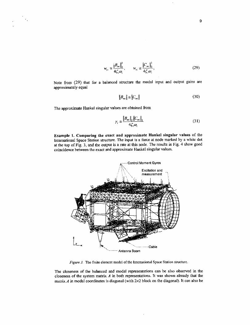
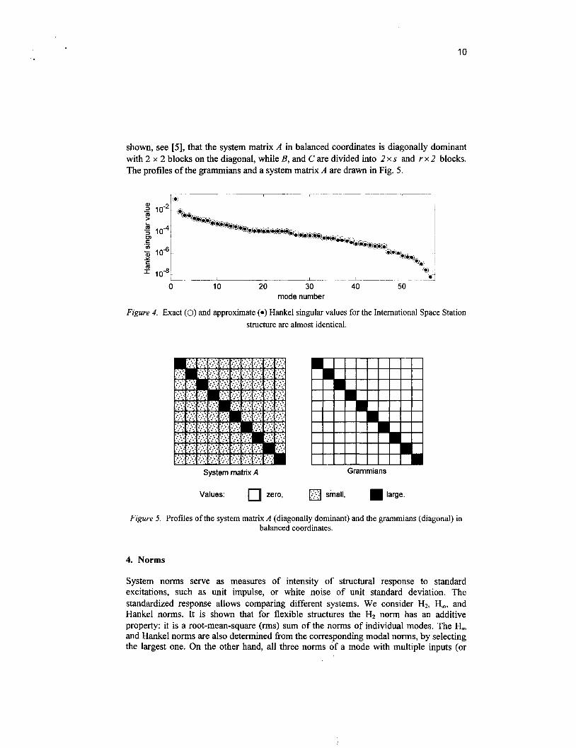
Example 1. Comparing the exact and approximate Hankel singular values of the International Space Station structure. The input is a force at node marked by a white dot at the top of Fig. 3, and the output is a rate at this node. The results in Fig. 4 show good coincidence between the exact and approximate Hankel singular values.
Control Moment Gyros
1 1 1 Excitation and ~
measurement
K--
I Cable Antenna Boom ---\ -~
Figure 3. The finite element model of the Intemational Space Station structure.
The closeness of the balanced and modal representations can be also observed in the closeness of the system matrix A in both representations. It was shown already that the matrix A in modal coordinates is diagonal (with 2x2 block on the diagonal). It can also be
10
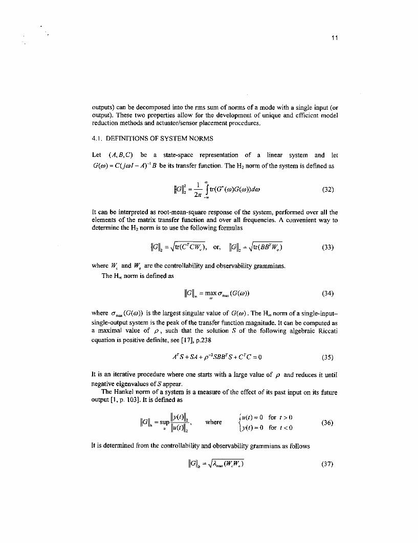
shown, see [ 5 ] , that the system matrix A in balanced coordinates is diagonally dominant with 2 x 2 blocks on the diagonal, while B, and C are divided into 2 x s and r x 2 blocks. The profiles of the grammians and a system matrix A are drawn in Fig. 5 .
0 10 20 30 40 50 mode number
Figure 4. Exact (0) and approximate ( 0 ) Hankel singular values for the International Space Station structure are almost identical.
System matrix A U U
Grammians
Values: zero, Q small, large.
Figure 5. Profiles of the system matrix A (diagonally dominant) and the grammians (diagonal) in balanced coordinates.
4. Norms
System norms serve as measures of intensity of structural response to standard excitations, such as unit impulse, or white noise of unit standard deviation. The standardized response allows comparing different systems. We consider H1, b, and Hankel norms. It is shown that for flexible structures the H2 norm has an additive property: it is a root-mean-square (rms) sum of the norms of individual modes. The H, and Hankel norms are also determined fkom the corresponding modal norms, by selecting the largest one. On the other hand, all three norms of a mode with multiple inputs (or
11
outputs) can be decomposed into the rms sum of norms of a mode with a single input (or output). These two properties allow for the development of unique and efficient model reduction methods and actuator/sensor placement procedures.
4.1. DEFINITIONS OF SYSTEM NORMS
Let ( A , B , C ) be a state-space representation of a linear system and let G(w) = C(jwZ - A)-' B be its transfer function. The H2 norm of the system is defined as
It can be interpreted as root-mean-square response of the system, performed over all the elements of the matrix transfer fbnction and over all fi-equencies. A convenient way to determine the H2 norm is to use the following formulas
where Wc and Wo are the controllability and observability grammians. The H, norm is defined as
where o,(G(w)) is the largest singular value of G(w) . The H, norm of a single-input- single-output system is the peak of the transfer fhction magnitude. It can be computed as a maximal value of p , such that the solution S of the following algebraic Riccati equation is positive definite, see [17], p.238
A T S + S A + p - 2 S B B T S + C T C = O (35)
It is an iterative procedure where one starts with a large value of p and reduces it until negative eigenvalues of S appear.
The Hankel norm of a system is a measure of the effect of its past input on its future output [ 1 , p. 1031. It is defined as
It is determined from the controllability and observability grammians as follows
12
where Am(.) denotes the largest eigenvalue. Thus, the Hankel norm of the system is therefore the largest Hankel singular value of the system, llGllh = y,- .
4.2. NORMS OF A SINGLE MODE
For structures in the modal representation each mode is independent, thus the norms of a single mode are independent as well. Consider the ith natural mode and its state-space representation (Ami, Bmi, Cmi) , see( 13). For this representation one obtains the following closed-form expression for the H2 norm, see [ 5 ] :
The Ha norm of a natural mode can be approximately expressed in the closed-form as follows:
In order to prove this, note that the largest amplitude of the mode is approximately at the ith natural fiequency, thus
The Hankel norm is approximately obtained f?om the following formula:
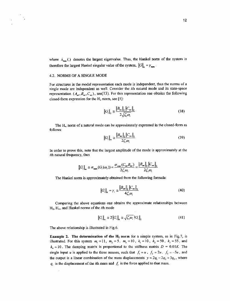
Comparing the above equations one obtains the approximate relationships between HZ, Ha, and Hankel norms of the ith mode
The above relationship is illustrated in Fig.6.
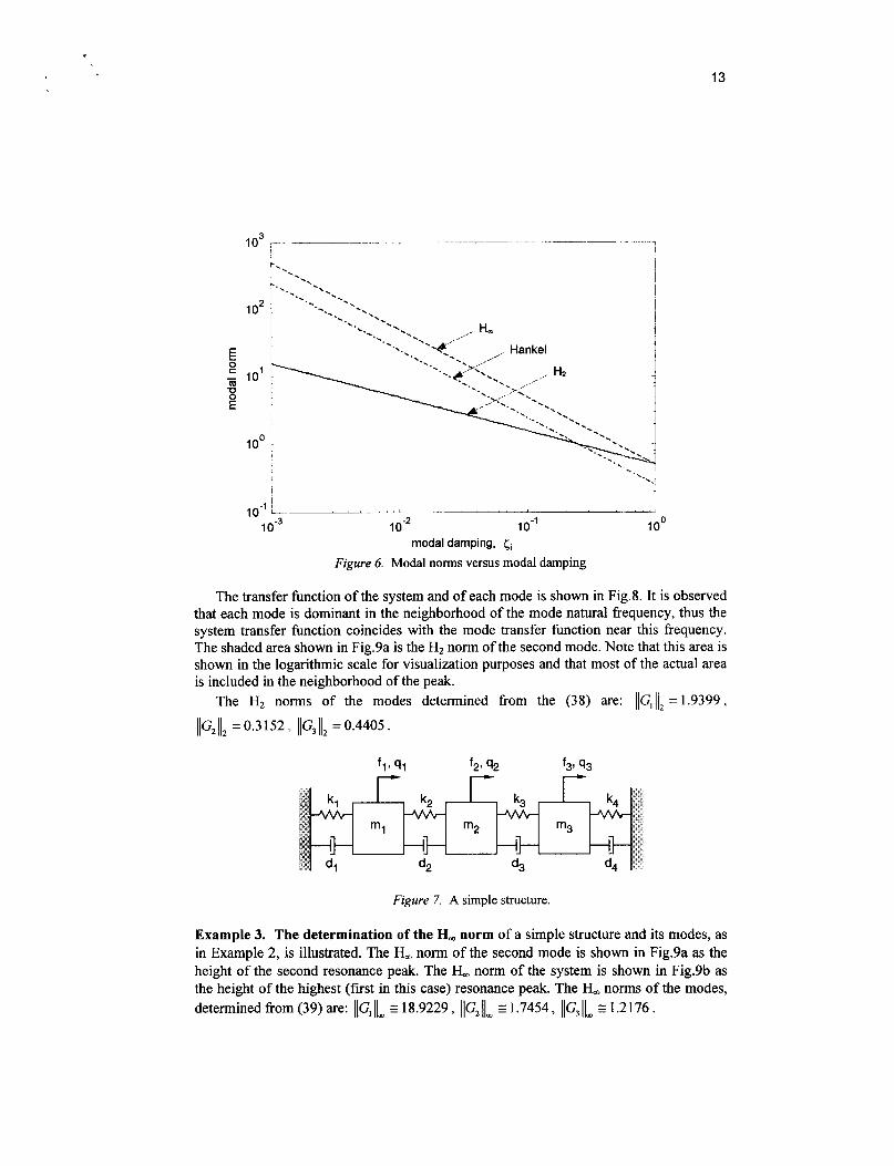
Example 2. The determination of the H2 norm for a simple system, as in Fig.7, is illustrated. For this system m, = 11, m, = 5 , m3 = 10, k, = 10, k, = 50, k, = 55, and k4 = 10. The damping matrix is proportional to the stiffness matrix D = 0.01K. The single input u is applied to the three masses, such that f ; = u , f, = 2u, f , = - 5 u , and the output is a linear combination of the mass displacements y = 2q, - 2q2 + 3q, , where qi is the displacement of the ith mass and is the force applied to that mass.
13
-. t --. !
10-1 i- , . , , , , , , I --. , , , 1 . , I , ,.-
1 o - ~ lo-* 1 0-1 loo modal damping, ci
Figure 6. Modal norms versus modal damping
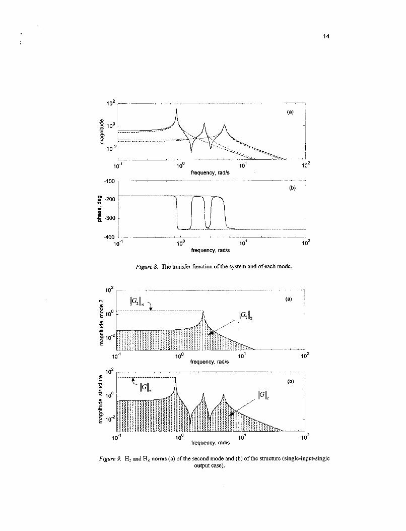
The transfer function of the system and of each mode is shown in Fig.8. It is observed that each mode is dominant in the neighborhood of the mode natural frequency, thus the system transfer function coincides with the mode transfer function near this frequency. The shaded area shown in Fig.9a is the H2 norm of the second mode. Note that this area is shown in the logarithmic scale for visualization purposes and that most of the actual area is included in the neighborhood of the peak.
The H2 norms of the modes determined from the (38) are: IlC, 1 1 2 = 1.9399,
f29 92 f39 93
Figure 7. A simple structure.
Example 3. The determination of the H, norm of a simple structure and its modes, as in Example 2, i s illustrated. The H, norm of the second mode is shown in Fig.9a as the height of the second resonance peak. The H, norm of the system is shown in Fig.9b as the height of the highest (first in this case) resonance peak. The H, norms of the modes, determined fiom (39) are: llG, [Im E 18.9229 , llG2 Ilm E 1.7454 , llG, [Im E 1.2 176 .
14
_ L l ,----L - u J -400 L ' ' I
1 0-1 1 oo 10' 1 o2 frequency, radls
Figure 8. The transfer function of the system and of each mode.
(a) I
I I -
I
I I
A-
1 0-1 1 oo I O 1 I o2 frequency, radls
10-I I O ' frequency, radls
1 oo 1 o2
Figure 9. H2 and H, norms (a) of the second mode and (b) of the structure (single-input-single output case).
15
Example 4. Determination of the H, norm of a single mode from the Ricccati equation (35). This norm is equal to the smallest positive parameter p for which the solution S of this equation is positive definite
Due to almost-independence of modes, the solution S of the Riccati equation is diagonally dominant, S z diag(s,, s2, ..., s,) , where, by inspection, one can find si as a solution of the following equation
where i = 1,2, ..., n , and A,,,; is given by Eq.(17), B,; is two-row block of B,
corresponding to block A,,,; of 4, and C,; is two-column block of C,: corresponding to block A,,,, of A,. For the balanced mode the Lyapunov equations (20) are
Introducing them to the previous equation we obtain
or, for a stable system
s, 2 --s,+p, P,’ 2 z o Yi
with two solutions sy) and s,!~)
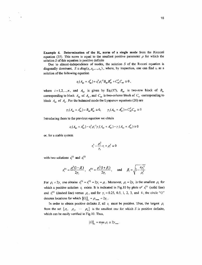
For pi = 2yi one obtains sy) = s,? = 2yi = pi . Moreover, pi = 2y; is the smallest pi for which a positive solution si exists. It is indicated in Fig.10 by plots of s,? (solid line) and s!~) (dashed line) versus pi , and for y; = 0.25, 0.5, 1, 2, 3, and 4 ; the circle “0”
denotes locations for which llG;II, = p,,, = 2y, .
from the set {p, , p2,
which can be easily verified in Fig. 10. Thus,
In order to obtain positive definite S, all si must be positive. Thus, the largest p,
p,,} is the smallest one for which S is positive definite, ...
16
“0 1 2 3 4 5 6 7 8 9 10
Pi
Figure 10. Solutions s,? (solid lines) and si(’) (dashed lines); note that pi = 2y, at locations marked “0”.
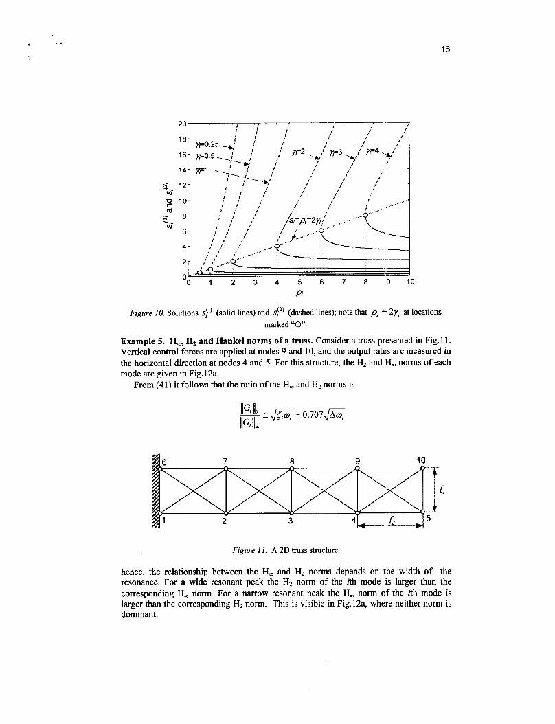
Example 5. k, H2 and Hankel norms of a truss. Consider a truss presented in Fig. 1 1. Vertical control forces are applied at nodes 9 and 10, and the output rates are measured in the horizontal direction at nodes 4 and 5. For this structure, the H2 and H, norms of each mode are given in Fig. 12a.
From (41) it follows that the ratio of the H, and H2 norms is
Figure 11. A 2D truss structure.
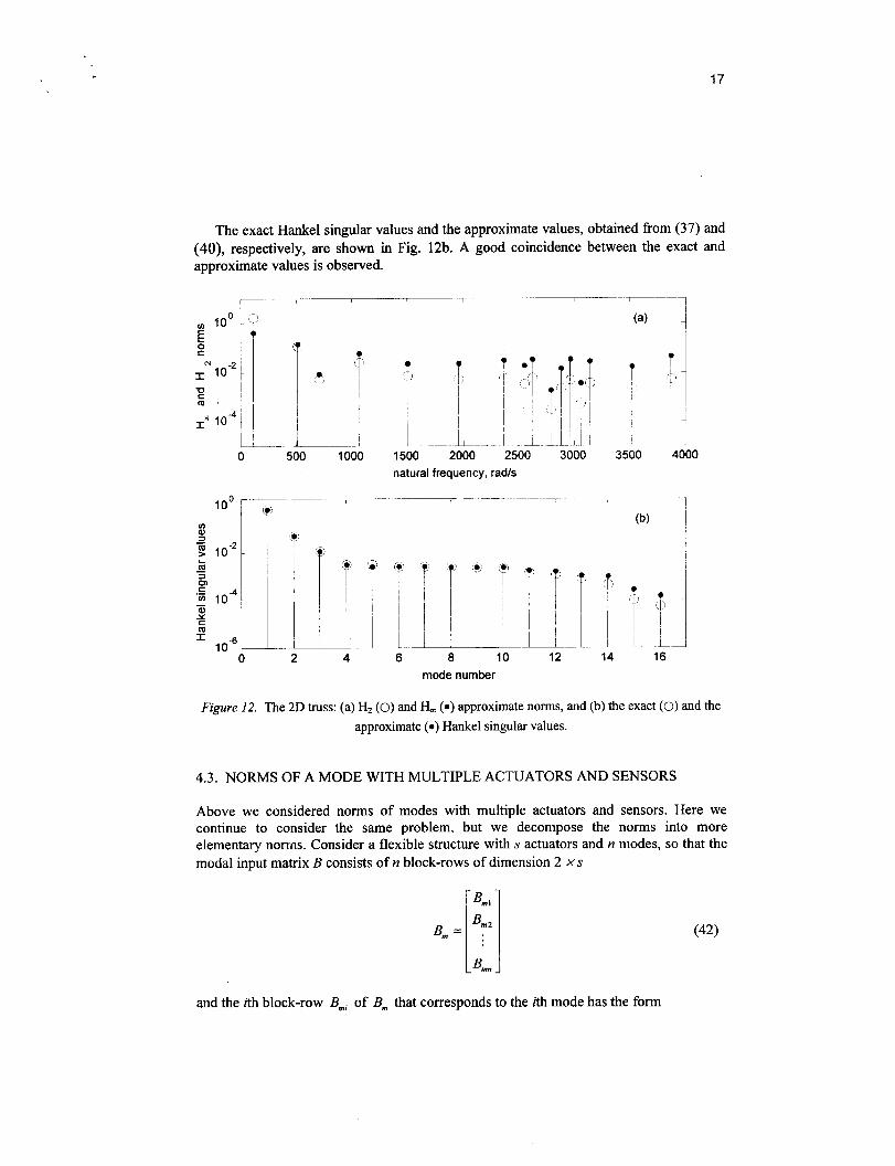
hence, the relationship between the H, and H2 norms depends on the width of the resonance. For a wide resonant peak the H2 norm of the zth mode is larger than the corresponding H, norm. For a narrow resonant peak the H, norm of the ith mode is larger than the corresponding H2 norm. This is visible in Fig. 12a, where neither norm is dominant.
17
The exact Hankel singular values and the approximate values, obtained from (37) and (40), respectively, are shown in Fig. 12b. A good coincidence between the exact and approximate values is observed.
m I
500 1000 1500 2000 2500 3000 3500 4000 natural frequency, radls
mode number
Figure 12. The 2D truss: (a) H2 (0) and H, (*) approximate norms, and (b) the exact (0) and the approximate ( 0 ) Hankel singular values.
4.3. NORMS OF A MODE WITH MULTIPLE ACTUATORS AND SENSORS
Above we considered norms of modes with multiple actuators and sensors. Here we continue to consider the same problem, but we decompose the norms into more elementary noms. Consider a flexible structure with s actuators and n modes, so that the modal input matrix B consists of n block-rows of dimension 2 x s
and the ith block-row Bmi of B, that corresponds to the ith mode has the form
18
where Bm, corresponds to the kth actuator at the ith mode. Similarly to the actuator properties one can derive sensor properties. For r sensors of
an n mode structure, the output matrix is as follows:
cm =[G, cm2 ... cmn], cm; = (44)
where Cmi is the output matrix of the ith mode, and Cmji is the 1 x2 block of thejth output at the ith mode.
Denote Gmlk the ith mode with kth actuator only, i.e. with the state-space representation ( 4j, Bmik, C m i ) . Let GmV be a structure with jth sensor only, i.e. with the state-space representation (Ai, Bmj,C,, ,+). The question arises as to how the norm of a mode with a single actuator or sensor corresponds to the norm of the same mode with multiple actuators or sensors.
We show that the H2, H,, and Hankel norms of the ith mode with a set of s actuators is the rms sum of the corresponding norms of the ith mode with a single actuator, i.e.,
where 11.11 denotes either HZ, H,, or Hankel norm. In order to show it, note that the norm of the ith mode with the kth actuator and the norm of the ith mode with all actuators are
where ai = 2&& for the H2 norm, a;. = 26iwi for the H, norm, and ai = 4 6 p i for the Hankel norm. But, from the definition of the norm and from (43) it follows that
Introducing the above equation to the previous one, one obtains (45). Similarly to the actuator properties one can derive sensor properties. For r sensors of
n modes the output matrix is as in Eq.(44). For this output matrix the Hz, H,, and Hankel norms of the ith mode of a structure with a set of r sensors is the rms sum of the corresponding norms of the mode with each single actuator from this set., Le.,
19
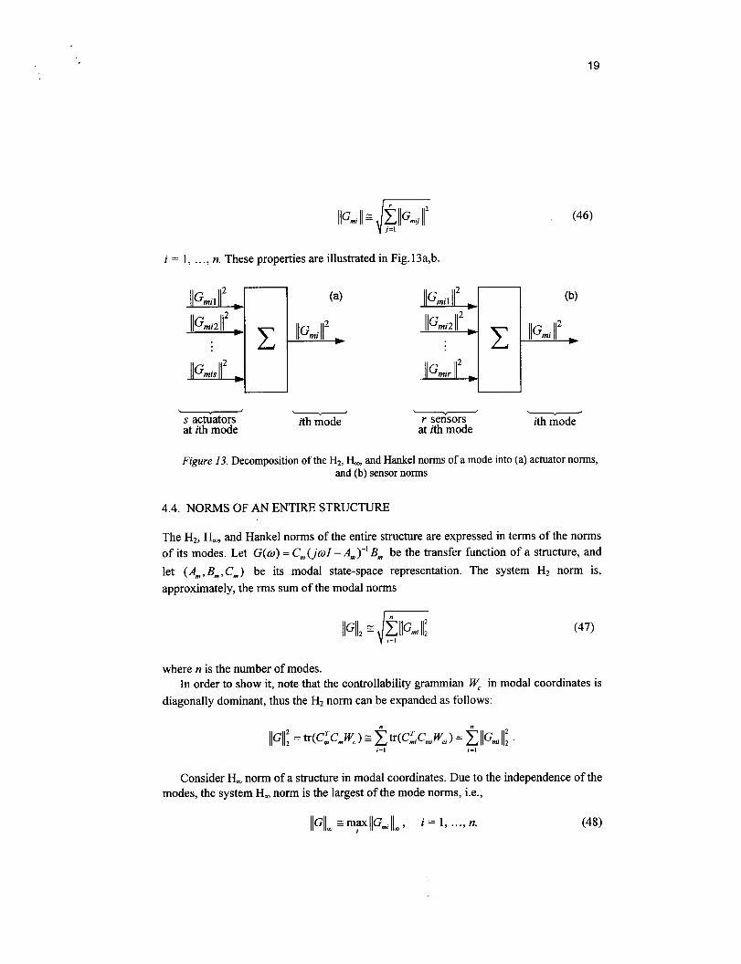
i = 1, . . ., n. These properties are illustrated in Fig. 13a,b.
I
s actuators at ith mode
- - r sensors ith mode at ith mode
Figure 13. Decomposition of the H2, &, and Hankel norms of a mode into (a) actuator norms, and (b) sensor norms
4.4. NORMS OF AN ENTIRE STRUCTURE
The HZ, H,, and Hankel norms of the entire structure are expressed in terms of the norms of its modes. Let G(w) = C,(jwI - A,)-' B, be the transfer function of a structure, and let (A,,,,Bm,Cm) be its modal state-space representation. The system H2 norm is, approximately, the rms sum of the modal norms
where n is the number of modes.
diagonally dominant, thus the H2 norm can be expanded as follows: In order to show it, note that the controllability grammian W, in modal coordinates is
Consider H, norm of a structure in modal coordinates. Due to the independence of the modes, the system H, norm is the largest of the mode norms, Le.,
20
This property says that for a single-input-single-output system the largest modal peak response determines the worst-case response.
The Hankel norm of the structure is the largest norm of its modes, Le.,
where y- is the largest Hankel singular value of the system.
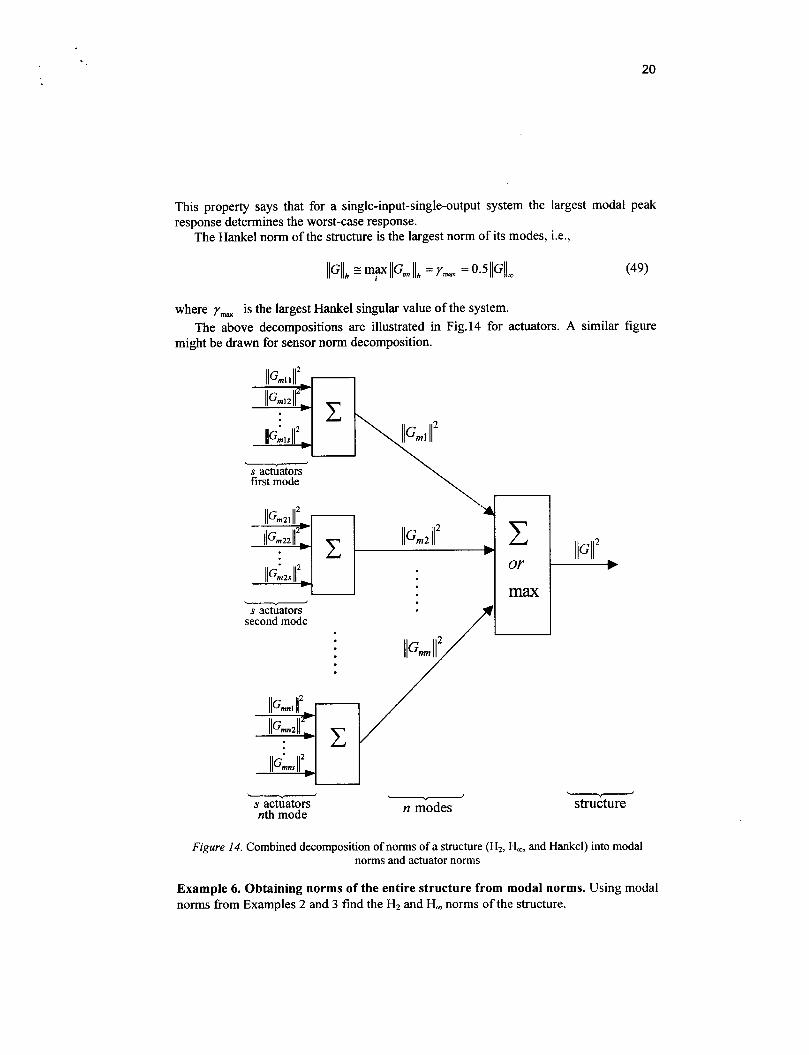
might be drawn for sensor norm decomposition. The above decompositions are illustrated in Fig.14 for actuators. A similar figure
- s actuators first mode
I -
s achiators second mode
I m a I
s actuators nth mode n modes
- structure
Figure 14. Combined decomposition of norms of a structure (H2, b, and Hankel) into modal norms and actuator norms
Example 6. Obtaining norms of the entire structure from modal norms. Using modal norms from Examples 2 and 3 find the H2 and Hm norms of the structure.
21
The H2 norm of the entire structure is represented by the shaded area in Fig.8b, which is approximately a sum of areas of each mode. We find fiom Eq.(47) that the approximate value of the system norm is the rms sum of modal norms, that is IIGl12 z J2.O14l2 +0.31522 +0.44052 = 2.0141. This value is equal to the exact value of the system norm.
The H, norm is the largest of the modal norms, see Eq.(48); using the results of Example 3 we found that the system norm is equal to the largest (first) modal norm, i.e., that llGllm = llGj ]Im z 18.9619 ; it is equal to the exact value of the system norm computed independently.
Example 7. Using norms to detect structural damage. We illustrate the application of Hz modal and sensor norms to determine damage locations. In particular, we localize damaged elements, and assess the modes particularly impacted by the damage.
Denote norm of the jth sensor of a healthy structure by IIGXh, 1 1 2 , and norm of the jth
sensor of a damaged structure by llGX4 ti2. The jth sensor index of the structural damage is defined as a weighted difference between the jth sensor norms of a healthy and damaged structure, Le.,
The sensor index reflects the impact of the structural damage on the jth sensor. Similarly, denote the norm of the ith mode of a healthy structure by llGmh, , and the
norm of the ith mode of a damaged structure by [lGmd, 1 1 2 . The ith mode index of the structural damage is defined as a weighted difference between the ith mode norm of a healthy and damaged structure, Le.,
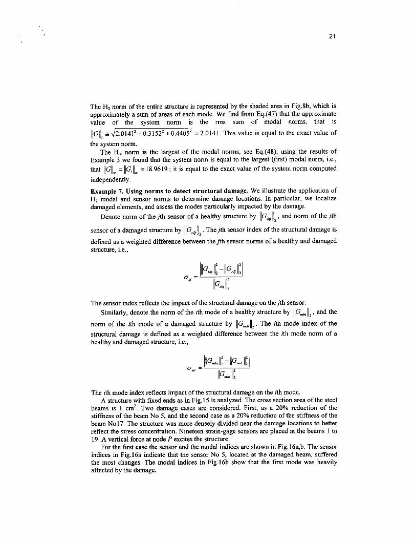
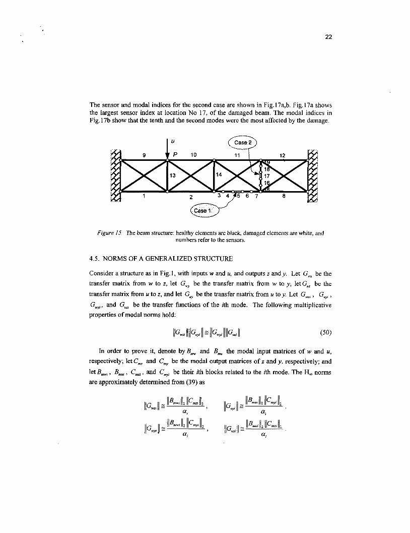
The ith mode index reflects impact of the structural damage on the ith mode. A structure with fKed ends as in Fig. 15 is analyzed. The cross section area of the steel
beams is 1 cm’. Two damage cases are considered. First, as a 20% reduction of the stiffness of the beam No 5 , and the second case as a 20% reduction of the stifkess of the beam No17. The structure was more densely divided near the damage locations to better reflect the stress concentration. Nineteen strain-gage sensors are placed at the beams 1 to 19. A vertical force at node P excites the structure.
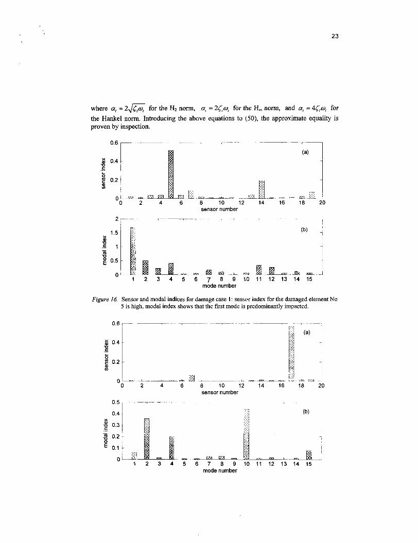
For the first case the sensor and the modal indices are shown in Fig. 16a,b. The sensor indices in Fig.16a indicate that the sensor No 5 , located at the damaged beam, suffered the most changes. The modal indices in Fig.16b show that the first mode was heavily affected by the damage.
22
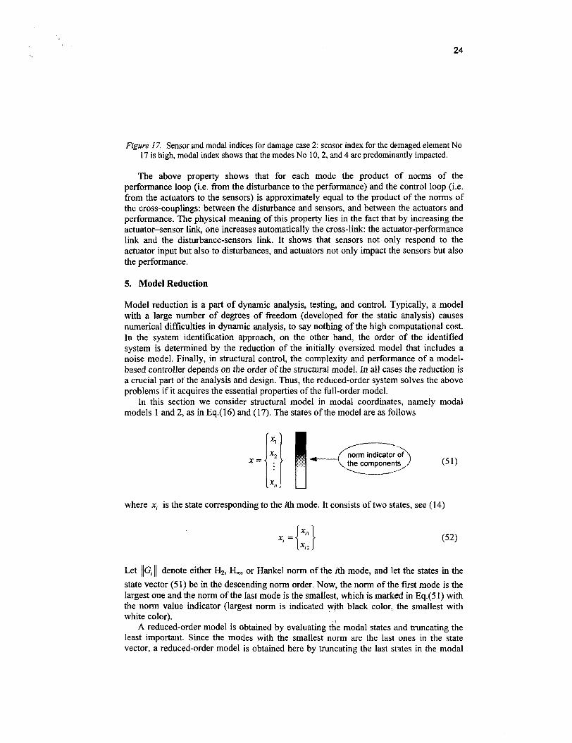
The sensor and modal indices for the second case are shown in Fig. 17a,b. Fig. 17a shows the largest sensor index at location No 17, of the damaged beam. The modal indices in Fig. 17b show that the tenth and the second modes were the most affected by the damage.
Figure 15. The beam structure: healthy elements are black, damaged elements are white, and numbers refer to the sensors.
4.5. NORMS OF A GENERALIZED STRUCTUW
Consider a structure as in Fig. 1, with inputs w and u, and outputs z and v. Let G,“, be the transfer matrix from w to z, let Gwy be the transfer matrix from w to y, let be the transfer matrix from u to z, and let Guy be the transfer matrix from u to v. Let G,,, , Guy, , G,,,, and G, be the transfer functions of the ith mode. The following multiplicative properties of modal norms hold:
In order to prove it, denote by B, and Bmu the modal input matrices of w and u,
respectively; let C, and C,, be the modal output matrices of z and y , respectively; and let B,, , B,, , C,, , and Cmp be their ith blocks related to the ith mode. The H, norms are approximately determined from (39) as
23
where al = 2 6 for the H2 norm, a, = 2<w, for the H, norm, and al = 4601, for the Hankel norm. Introducing the above equations to (50), the approximate equality is proven by inspection.
17-7- ----- 17.- p-7-y
8 0.4
b e 0.2 %
1 0 1-s UD- I rL 0 2 4 6 8 10 12 14 16 18 20
sensor number
2 - - - - 7 - 7-j--, r p - 7 ~ 7 - r 1 , (b) 1.5
.E 1
0.5
G -0
m -0
i -
1 2 3 4 5 6 7 8 9 1 0 1 1 1 2 1 3 1 4 1 5 mode number
Figure 16. Sensor and modal indices for damage case 1 : sensor index for the damaged element No 5 is high, modal index shows that the first mode is predominantly impacted.
0.6 r---
e 0.2 (u In : I
0 L. 0 12 14 16 18 20
sensor number
051 - r - 7 1
0 4
2 0.3 X
.- - g 0.2
E 0.1 0
'I 2 3 4 5 6 7 8 9 1 0 1 1 1 2 1 3 1 4 1 5 mode number
24
Figure 17. Sensor and modal indices for damage case 2: sensor index for the &maged element No 17 is high, modal index shows that the modes No 10,2, and 4 are predominantly impacted.
The above property shows that for each mode the product of norms of the performance loop (i.e. fiom the disturbance to the performance) and the control loop (Le. from the actuators to the sensors) is approximately equal to the product of the norms of the cross-couplings: between the disturbance and sensors, and between the actuators and performance. The physical meaning of this property lies in the fact that by increasing the actuator-sensor link, one increases automatically the cross-link: the actuator-performance link and the disturbance-sensors link. It shows that sensors not only respond to the actuator input but also to disturbances, and actuators not only impact the sensors but also the performance.
5. Model Reduction
Model reduction is a part of dynamic analysis, testing, and control. Typically, a model with a large number of degrees of fteedom (developed for the static analysis) causes numerical difficulties in dynamic analysis, to say nothing of the high computational cost. In the system identification approach, on the other hand, the order of the identified system is determined by the reduction of the initially oversized model that includes a noise model. Finally, in structural control, the complexity and performance of a model- based controller depends on the order of the structural model. In all cases the reduction is a crucial part of the analysis and design. Thus, the reduced-order system solves the above problems if it acquires the essential properties of the full-order model.
In this section we consider structural model in modal coordinates, namely modal models 1 and 2, as in Eq.(16) and (17). The states ofthe model are as follows
where x, is the state corresponding to the ith mode. It consists of two states, see (14)
Let llG, 11 denote either Hz, H,, or Hankel norm of the rth mode, and let the states in the state vector (5 1) be in the descending norm order. Now, the norm of the first mode is the largest one and the norm of the last mode is the smallest, which is marked in Eq.(5 1 ) with the norm value indicator (largest norm is indicated with black color. the smallest with white color).
A reduced-order model is obtained by evaluating the modal states and truncating the least important. Since the modes with the smallest norm are the last ones in the state vector, a reduced-order model is obtained here by truncating the last states in the modal
25
vector. How many of them? It depends on the system requirements, and is up to design engineer to check the reduced model accuracy. Let(4,,Bm,Cm) be the modal representation corresponding to the modal state vector x as in (51). Let x be partitioned as follows:
x = { : ) (53)
where x, is the vector of the retained states, and x, is a vector of truncated states. If there are k < n retained modes, x, is a vector of 2k states, and x, is a vector of 2(n-k) states. Let the state triple (A, , B, , C, ) be partitioned accordingly,
The reduced model is obtained by deleting the last 2(n-k) rows of An, and B,,, , and the last 2(n-k) columns of A,,, and C, .
Modal reduction by a truncation of a stable model always produces a stable reduced model, since the poles of the reduced model have not been changed.
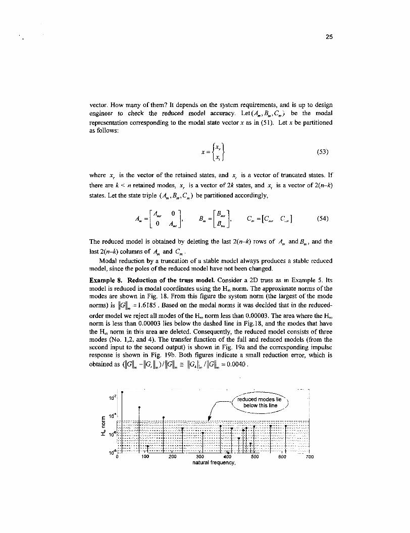
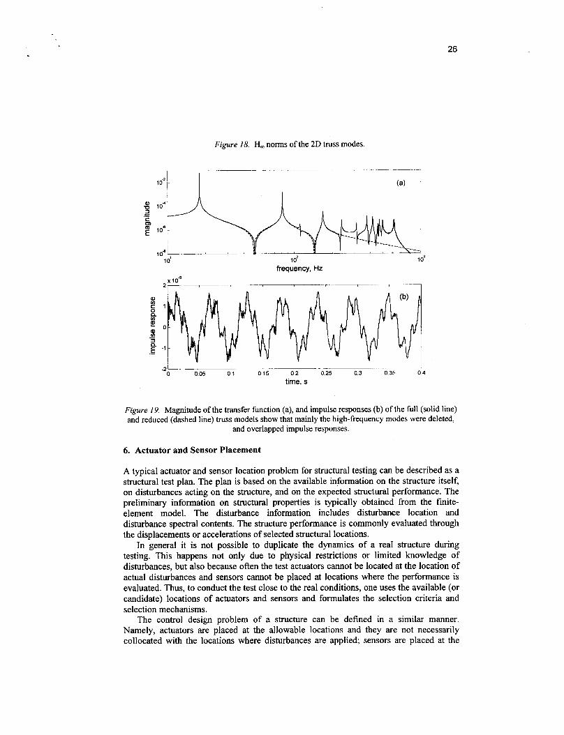
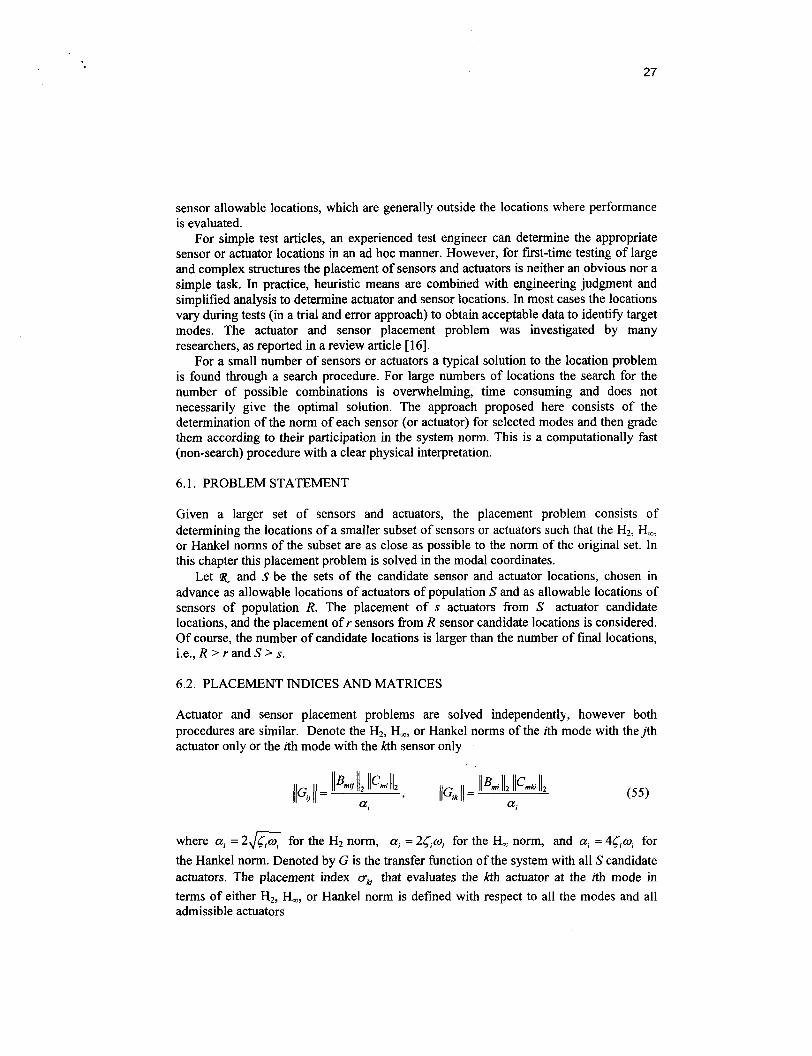
Example 8. Reduction of the truss model. Consider a 2D truss as in Example 5. Its model is reduced in modal coordinates using the H, norm. The approxirnate norms of the modes are shown in Fig. 18. From this figure the system norm (the largest of the mode norms) is IlGll, = 1.6185 . Based on the modal norms it was decided that in the reduced- order model we reject all modes of the H, norm less than 0.00003. The area where the H, norm is less than 0.00003 lies below the dashed line in Fig.18, and the modes that have the H, norm in this area are deleted. Consequently, the reduced model consists of three modes (No. 1,2, and 4). The transfer function of the full and reduced models (from the second input to the second output) is shown in Fig. 19a and the corresponding impulse response is shown in Fig. 19b. Both figures indicate a small reduction error, which is obtained as (IlGll, - llGrIlm)/llGllm G IIG,llm /IIGllm = 0.0040 .
natural frequency,
26
Figure 18. H, norms of the 2D truss modes.
frequency, Hz
. L I - L - .
0 05 0 1 0 15 0 2 0 25 03 0 35 0 4 -2 0
time, s
Figure 19. Magnitude of the transfer function (a), and impulse responses (b) of the full (solid line) and reduced (dashed line) truss models show that mainly the high-frequency modes were deleted,
and overlapped impulse responses.
6. Actuator and Sensor Placement
A typical actuator and sensor location problem for structural testing can be described as a structural test plan. The plan is based on the available information on the structure itself, on disturbances acting on the structure, and on the expected structural performance. The preliminary information on structural properties is typically obtained from the fmite- element model. The disturbance information includes disturbance location and disturbance spectral contents. The structure performance is commonly evaluated through the displacements or accelerations of selected structural locations.
In general it is not possible to duplicate the dynamics of a rea1 structure during testing. This happens not only due to physical restrictions or limited knowledge of disturbances, but also because often the test actuators cannot be located at the location of actual disturbances and sensors cannot be placed at locations where the performance is evaluated. Thus, to conduct the test close to the real conditions, one uses the available (or candidate) locations of actuators and sensors and formulates the selection criteria and selection mechanisms.
The control design problem of a structure can be defined in a similar manner. Namely, actuators are placed at the allowable locations and they are not necessarily collocated with the locations where disturbances are applied; sensors are placed at the
27
sensor allowable locations, which are generally outside the locations where performance is evaluated.
For simple test articles, an experienced test engineer can determine the appropriate sensor or actuator locations in an ad hoc manner. However, for first-time testing of large and complex structures the placement of sensors and actuators is neither an obvious nor a simple task. In practice, heuristic means are combined with engineering judgment and simplified analysis to determine actuator and sensor locations. In most cases the locations vary during tests (in a trial and error approach) to obtain acceptable data to identify target modes. The actuator and sensor placement problem was investigated by many researchers, as reported in a review article [ 161.
For a small number of sensors or actuators a typical solution to the location problem is found through a search procedure. For large numbers of locations the search for the number of possible combinations is overwhelming, time consuming and does not necessarily give the optimal solution. The approach proposed here consists of the determination of the norm of each sensor (or actuator) for selected modes and then grade them according to their participation in the system norm. This is a computationally fast (non-search) procedure with a clear physical interpretation.
6.1. PROBLEM STATEMENT
Given a larger set of sensors and actuators, the placement problem consists of determining the locations of a smaller subset of sensors or actuators such that the €IZ, H,, or Hankel norms of the subset are as close as possible to the norm of the original set. In this chapter this placement problem is solved in the modal coordinates.
and S be the sets of the candidate sensor and actuator locations, chosen in advance as allowable locations of actuators of population S and as allowable locations of sensors of population R. The placement of s actuators from S actuator candidate locations, and the placement of r sensors from R sensor candidate locations is considered. Of course, the number of candidate locations is larger than the number of final locations, i.e., R > r and S
Let
s.
6.2. PLACEMENT INDICES AND MATRICES
Actuator and sensor placement problems are solved independently, however both procedures are similar. Denote the H2, H,, or Hankel norms of the ith mode with thejth actuator only or the ith mode with the kth sensor only
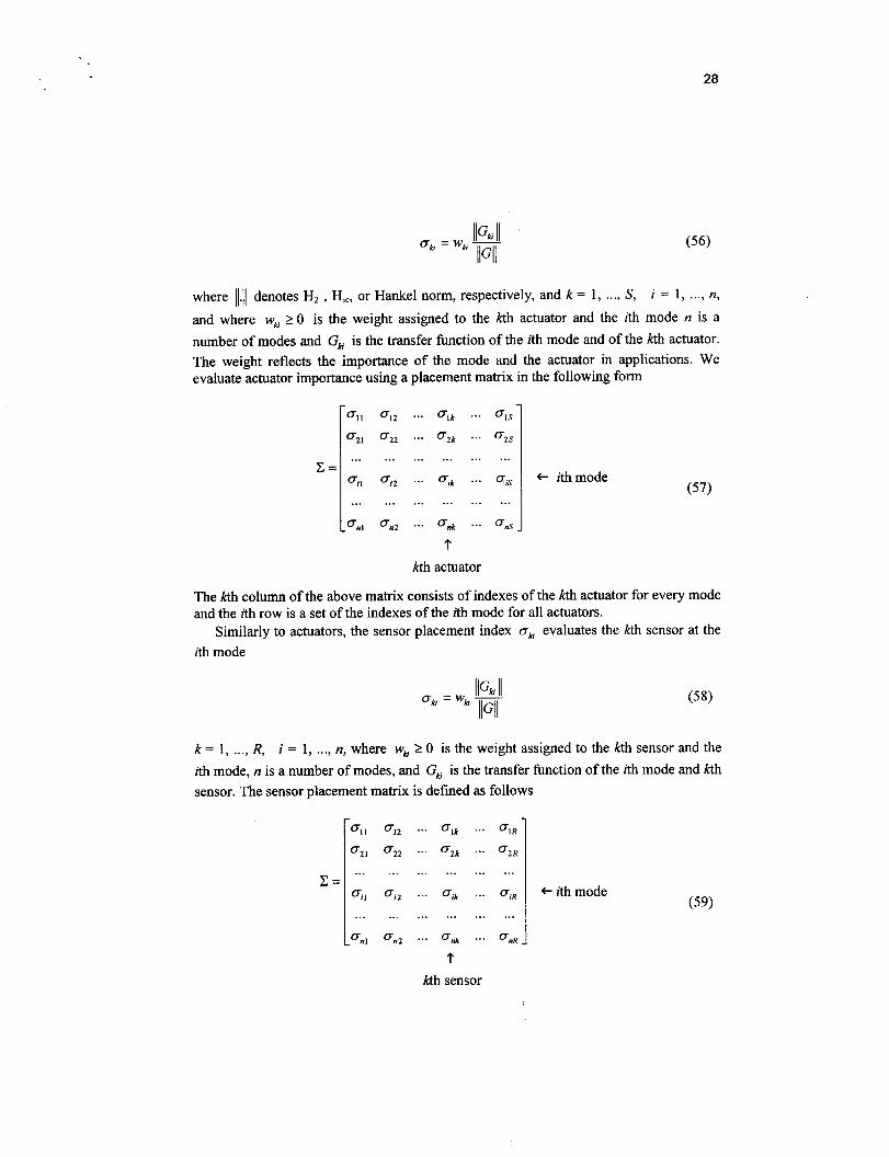
where a, = 2% for the H2 norm, ai = 2<pi for the H, norm, and ai = 4<pi for the Hankel norm. Denoted by G is the transfer function of the system with all S candidate actuators. The placement index a, that evaluates the kth actuator at the ith mode in terms of either HZ, H,, or Hankel norm is defined with respect to all the modes and all admissible actuators
28
where 11.11 denotes H2 . H,, or Hankel norm, respectively, and k = 1, .... S, i = 1, .... n,
and where w, 20 is the weight assigned to the kth actuator and the ith mode n is a number of modes and Gk is the transfer function of the ith mode and of the kth actuator. The weight reflects the importance of the mode and the actuator in applications. We evaluate actuator importance using a placement matrix in the following form
c =
a,, a,* ... Olk ... (TIS
a,, ... cT2k ...
a,, a,, ... a, ... (Tis
a,, a,, ... a, ... an,s
. . . . . . . . . . . . . . . . . .
. . . . . . . . . . . . . . . . . .
t kth actuator
+ ithmode (57)
The kth column of the above matrix consists of indexes of the kth actuator for every mode and the ith row i s a set of the indexes of the ith mode for all actuators.
Similarly to actuators, the sensor placement index akj evaluates the kth sensor at the ith mode
k = 1, .... R, i = 1, .... n, where w, 2 0 is the weight assigned to the kth sensor and the zth mode, n is a number of modes, and G, is the transfer function of the zth mode and kth sensor. The sensor placement matrix is defined as follows
c =
- a,, ... CTlk ... a,, a,, ... ...
a,, ... a,, ... aiR
. . . . . . . . . . . . . . .
. . . . . . . . . . . . ... I
ith mode (59)
29
where the kth column consists of indexes of the kth sensor for every mode and the ith row is a set of the indexes of the ith mode for all sensors.
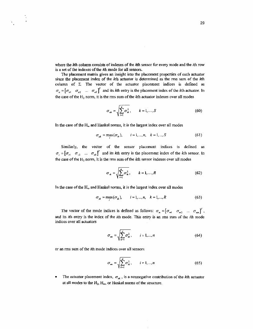
The placement matrix gives an insight into the placement properties of each actuator since the placement index of the kth actuator is determined as the rms s u m of the kth column of C. The vector of the actuator placement indices is defined as aa = [a,, aaoZ ... and its kth entry is the placement index of the kth actuator. In the case of the H2 norm, it is the rms sum of the kth actuator indexes over all modes
In the case of the H, and Hankel norms, it is the largest index over all modes
a,k = mv(aik) , i = 1 ,..., n, k = 1 ,..., S (61) I
Similarly, the vector of the sensor placement indices is defined as ... 0 . ~ 1 ~ and its kth entry is the placement index of the kth sensor. In a, = [os,
the case of the H2 norm, it is the rms sum of the kth sensor indexes over all modes as2
In the case of the H, and Hankel norms, it is the largest index over all modes
ask = mp(oik) , i = 1 ,..., n, k = 1 ,..., R (63)
The vector of the mode indices is defined as follows: a, =[a,, a,, ... a,,I7, and its ith entry is the index of the ith mode. This entry is an rms sum of the ith mode indices over all actuators
a,,,, = @ a i , i = l , ..., n k=l
or an rms sum of the ith mode indices over all sensors
a,,,, = & a i , i = l , ..., n
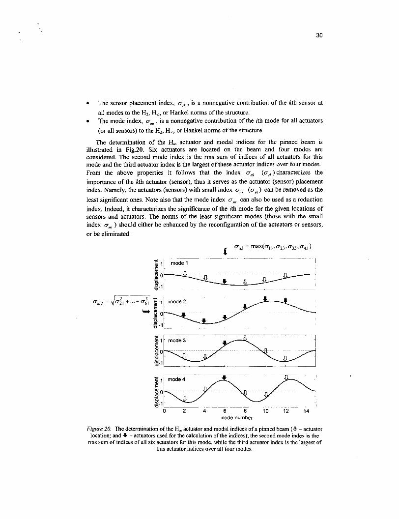
The actuator placement index, 0, , is a nonnegative contribution of the kth actuator at all modes to the H1, H,, or Hankel norms of the structure.
30
0 The sensor placement index, o , ~ ~ , is a nonnegative contribution of the kth sensor at all modes to the H2, H,, or Hankel norms of the structure. The mode index, a,,,, , is a nonnegative contribution of the zth mode for all actuators (or all sensors) to the HZ, H,, or Hankel norms of the structure.
The determination of the H, actuator and modal indices for the pinned beam is illustrated in Fig.20. Six actuators are located on the beam and four modes are considered. The second mode index is the rms sum of indices of all actuators for this mode and the third actuator index is the largest of these actuator indices over four modes. From the above properties it follows that the index oak (a,)characterizes the importance of the kth actuator (sensor), thus it serves as the actuator (sensor) placement index. Namely, the actuators (sensors) with small index a, (a,) can be removed as the least significant ones. Note also that the mode index a,,,, can also be used as a reduction index. Indeed, it characterizes the significance of the ith mode for the given locations of sensors and actuators. The norms of the least significant modes (those with the small index a,,,, ) should either be enhanced by the reconfiguration of the actuators or sensors, or be eliminated.
am2 = K+ ...+
0 2 4 6 8 10 12 14 node number
Figure 20. The determination of the H, actuator and modal indices of a pinned beam (0 - actuator location; and * - actuators used for the calculation of the indices); the second mode index is the
rms sum of indices of all six actuators for this mode, while the third actuator index is the largest of this actuator indices over all four modes.
31
Actuator Sensor (fixed location) (variable location)
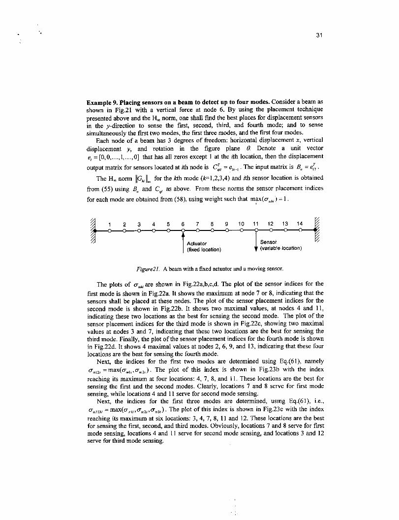
Example 9. Placing sensors on a beam to detect up to four modes. Consider a beam as shown in Fig.21 with a vertical force at node 6. By using the placement technique presented above and the H, norm, one shall find the best places for displacement sensors in the y-direction to sense the first, second, third, and fourth mode; and to sense simultaneously the first two modes, the first three modes, and the first four modes.
Each node of a beam has 3 degrees of freedom: horizontal displacement x, vertical displacement y , and rotation in the figure plane 8. Denote a unit vector e, = [O,O,. . ., 1,. . . ,O] that has all zeros except 1 at the ith location, then the displacement output matrix for sensors located at ith node is Ci, = e,,_, . The input matrix is Bo = e; .
The H, norm IlG, 11, for the kth mode (k=l,2,3,4) and ith sensor location is obtained from (55) using Bo and C,, as above. From these norms the sensor placement indices for each mode are obtained from (58), using weight such that max(o,,, ) = 1 .
FigureZI. A beam with a fixed actuator and a moving sensor.
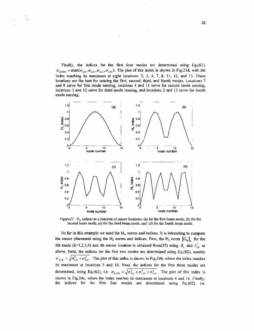
The plots of a,, are shown in Fig.22a,b,c,d. The plot of the sensor indices for the first mode is shown in Fig.22a. It shows the maximum at node 7 or 8, indicating that the sensors shall be placed at these nodes. The plot of the sensor placement indices for the second mode is shown in Fig.22b. It shows two maximal values, at nodes 4 and 11, indicating these two locations as the best for sensing the second mode. The plot of the sensor placement indices for the third mode is shown in Fig.22c, showing two maximal values at nodes 3 and 7, indicating that these two locations are the best for sensing the third mode. Finally, the plot of the sensor placement indices for the fourth mode is shown in Fig.22d. It shows 4 maximal values at nodes 2, 6, 9, and 13, indicating that these four locations are the best for sensing the fourth mode.
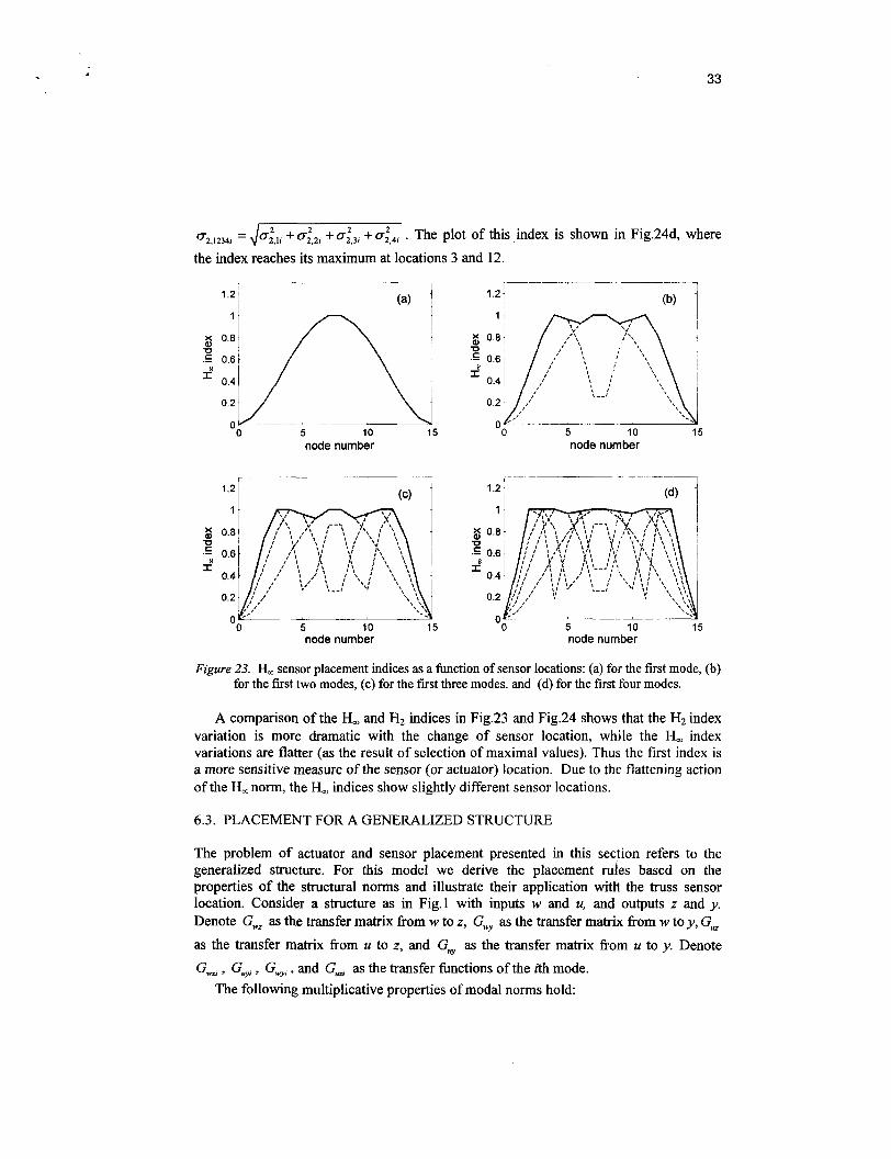
Next, the indices for the first two modes are determined using Eq.(61), namely omlz, = max(om,,,am2,). The plot of this index is shown in Fig.23b with the index reaching its maximum at four locations: 4, 7, 8, and 11. These locations are the best for sensing the first and the second modes. Clearly, locations 7 and 8 serve for first mode sensing, while locations 4 and 11 serve for second mode sensing.
Next, the indices for the first three modes are determined, using Eq.(61), Le., = max(a,,,,a,,,,o,,,). The plot of this index is shown in Fig.23~ with the index
reaching its maximum at six locations: 3, 4, 7, 8, 11 and 12. These locations are the best for sensing the first, second, and third modes. Obviously, locations 7 and 8 serve for first mode sensing, locations 4 and 11 serve for second mode sensing, and locations 3 and 12 serve for third mode sensing.
32
Finally, the indices for the first four modes are determined using Eq.(61), omlU4, = max(o,,, ,om2, ,om3,,om4,). The plot of this index is shown in Fig.23d, with the index reaching its maximum at eight locations: 2, 3, 4, 7, 8, 11, 12, and 13. These locations are the best for sensing the first, second, third, and fourth modes. Locations 7 and 8 serve for first mode sensing, locations 4 and 11 serve for second mode sensing, locations 3 and 12 serve for third mode sensing, and locations 2 and 13 serve for fourth mode sensing.
~~ __ __
0 5 10 15 0 5 10 15 node number node number
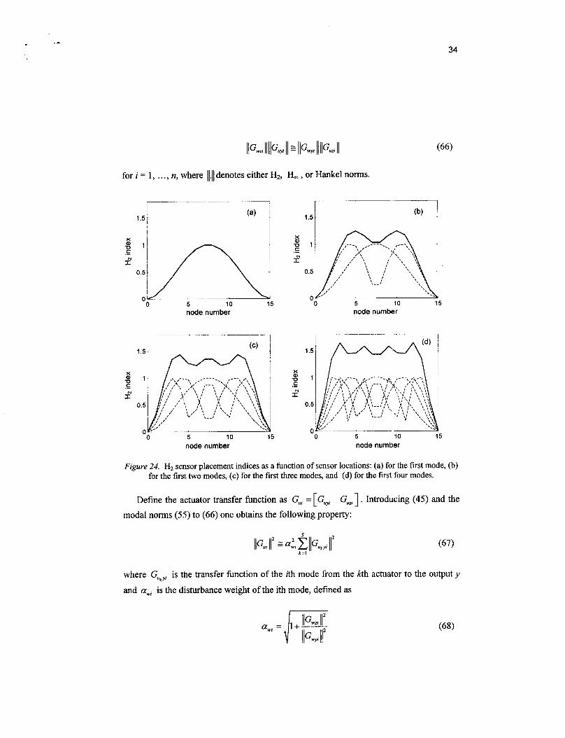
Fzgure22 H, indices as a function of sensor locations: (a) for the first beam mode, (b) for the second beam mode, (c) for the third beam mode, and (d) for the fourth beam mode.
So far in this example we used the H, norms and indices. It is interesting to compare the sensor placement using the H2 norms and indices. First, the H2 norm llGkII, for the kth mode (k=1,2,3,4) and ith sensor location is obtained fiom(55) using Bo and C,,, as above. Next, the indices for the first two modes are determined using Eq.(62), namely cr2,12, = ,/-. The plot of this index is shown in Fig.24b, where the index reaches its maximum at locations 5 and 10. Next, the indices for the first three modes are determined, using Eq.(62), i.e. CT~,,~,, = ,/-. The plot of this index is shown in Fig.24c, where the index reaches its maximum at locations 4 and 11. Finally, the indices for the first four modes are determined using Eq.(62), i.e.
33
C T ~ , ~ ~ ~ ~ ~ = Ja,,,, 2 +&, +u& +& . The plot of this index is shown in Fig.24d, where
the index reaches its maximum at locations 3 and 12.
node number
7 ' 1
1.21 (a i
"0 5 10 15 node number
0 5 10 15 0 5 10 15 node number node number
Figure 23. H, sensor placement indices as a function of sensor locations: (a) for the first mode, (b) for the first two modes, (c) for the first three modes, and (d) for the first four modes.
A comparison of the H, and H2 indices in Fig.23 and Fig.24 shows that the H2 index variation is more dramatic with the change of sensor location, while the H, index variations are flatter (as the result of selection of maximal values). Thus the first index is a more sensitive measure of the sensor (or actuator) location. Due to the flattening action of the H, norm, the H, indices show slightly different sensor locations.
6.3 . PLACEMENT FOR A GENERALIZED STRUCTURE
The problem of actuator and sensor placement presented in this section refers to the generalized structure. For this model we derive the placement rules based on the properties of the structural norms and illustrate their application with the truss sensor location. Consider a structure as in Fig.1 with inputs w and u, and outputs z and y. Denote Gwz as the transfer matrix fkom w to z, Gwy as the transfer matrix fkom w toy, G, as the transfer matrix fkom u to z, and Guy as the transfer matrix fiom u to y. Denote G,,, , Guy , Gwy3 , and G, as the transfer functions of the ith mode.
The following multiplicative properties of modal norms hold:
34
; X I ly$ 051
I
~ - _. 15
0 0 5 10
node number 0 5 10 15
node number
" 0 5 10 15
node number node number
Figure 24. H2 sensor placement indices as a function of sensor locations: (a) for the first mode, (b) for the first two modes, (c) for the first three modes, and (d) for the first four modes.
Define the actuator transfer function as Cui = [G,,$ Gu,]. Introducing (45) and the modal norms (55) to (66) one obtains the following property:
where G,,kyi is the transfer fbnction of the ith mode from the kth actuator to the output y
and a,, is the disturbance weight of the ith mode, defined as
35
To show it, note that
Note also that from Eq.(45) one obtains
where Gukzj is the transfer function of the ith mode from the kth actuator to the performance z. Introducing the above equations to Eq.(69) we obtained the following
relationship: llG,,i 112 = k( llGUkzi l(2 + llGukr l(2 ) . Next, Eq.(66) gives k=l
which, introduced to the previous equation gives (67). Note that the disturbance weight a,, does not depend on the actuator location: it characterizes structural dynamics caused by the disturbances w.
Similarly, one obtains the additive property of the sensor locations of a generalized structure. Define the sensor transfer h c t i o n as Gyi =[Gw. Guyl ] , thus
IIGp 112 E IIGwy, 112 + ilGuYl 1 1 2 , then the following property holds:
where
is the performance weight of the ith mode. Note that the performance weight azj characterizes part of the structural dynamics that is observed at the performance output; hence, it does not depend on the sensor location.
The above properties are the basis of the actuator and sensor search procedure of a generalized structure. The actuator index evaluates the actuator usefulness in test, and is defined as follows:
36
o,, ... aZk ... azs
where llGu 112 = IlG,,,, 11’ + llG, 112, while the sensor index is
. . . . . . . . . . . . . . . . . . ai, ai, ... a, ... o,
where llGy 112 = [IC, 112 + IlGWY 112 . The indices are the building blocks of the actuator placement matrix C
+ ith mode (74) . . . . . . . . . . . . . . .
=“I O n 2 ..’ onk ”’ ... 7
kth actuator
and a similar matrix for sensor placement. The placement index of the kth actuator (sensor) is determined from the kth column of
C. In the case of the H2 norm, it is the rms sum of the kth actuator indexes over all modes,
k = 1, .... S or R , and in the case of the H, and Hankel norms it is the largest index over all modes
i = l , .... n, k-1, .... S o r R . This property shows that the index for the set of sensorslactuators is determined from
the indexes of each individual sensor or actuator. ‘This decomposition allows for the evaluation of an individual sensorlactuator through its participation in the performance of the whole set of sensorslactuators.
Example 10. Sensor placement for a generalized structure. Consider the 3D truss as in Fig.25. The disturbance w is applied at node 7 in the horizontal direction. The
37
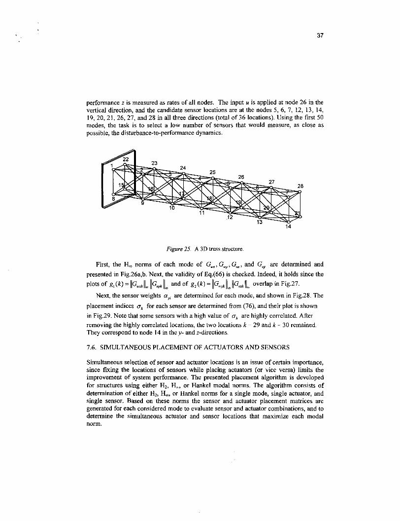
performance z is measured as rates of all nodes. The input u is applied at node 26 in the vertical direction, and the candidate sensor locations are at the nodes 5 , 6, 7, 12, 13, 14, 19, 20, 21, 26, 27, and 28 in all three directions (total of 36 locations). Using the first 50 modes, the task is to select a low number of sensors that would measure, as close as possible, the disturbance-to-performance dynamics.
Figure 25. A 3D truss structure.
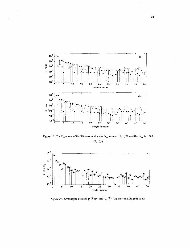
First, the H, norms of each mode of G,,, Gw,, G,, and G, are determined and presented in Fig.26a,b. Next, the validity of Eq.(66) is checked. Indeed, it holds since the plots Of gl ( k ) = (I'wzk Ilm llGuyk Ilm and Of g2 ( k ) = IIGwyk (Im llGuzk (Im Overlap in Fig'27'
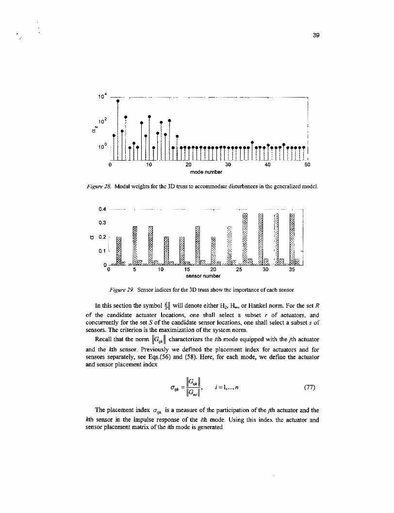
Next, the sensor weights a,# are determined for each mode, and shown in Fig.28. The placement indices ok for each sensor are determined from (76), and their plot is shown in Fig.29. Note that some sensors with a high value of o, are highly correlated. After removing the highly correlated locations, the two locations k = 29 and k = 30 remained. They correspond to node 14 in they- and z-directions.
7.6. SIMULTANEOUS PLACEMENT OF ACTUATORS AND SENSORS
Simultaneous selection of sensor and actuator locations is an issue of certain importance, since fixing the locations of sensors while placing actuators (or vice versa) limits the improvement of system performance. The presented placement algorithm is developed for structures using either HZ, H,, or Hankel modal norms. The algorithm consists of determination of either H1, H,, or Hankel norms for a single mode, single actuator, and single sensor. Based on these norms the sensor and actuator placement matrices are generated for each considered mode to evaluate sensor and actuator combinations, and to determine the simultaneous actuator and sensor locations that maximize each modal norm.
38
0 5 10 15 20 25 30 35 40 45 50 mode number
, --I--, I-- ,
I 1 1 2 1
5 10 15 20 25 30 35 40 45 50 mode number
Figure 26. The H, norms of the 3D truss modes: (a) G,, ( 0 ) and G,,,, (0); ard (b) Gwy ( 0 ) and
G, (0)
mode number
Figure 27. Overlapped plots of g, ( k ) ( 0 ) and g, ( k ) (0) show that Eq.(66) holds.
39
lo4
IO2 N d
0
i! a I
mode number
Figure 28. Modal weights for the 3D truss to accommodate disturbances in the generalized model.
sensor number
Figure 29. Sensor indices for the 3D truss show the importance of each sensor.
In this section the symbol 11.11 will denote either HZ, H,, or Hankel norm. For the set R of the candidate actuator locations, one shall select a subset r of actuators, and concurrently for the set S of the candidate sensor locations, one shall select a subset s of sensors. The criterion is the maximization of the system norm.
Recall that the norm ~ ~ G o k ~ ~ characterizes the ith mode equipped with thejth actuator and the kth sensor. Previously we defined the placement index for actuators and for sensors separately, see Eqs.(56) and (58). Here, for each mode, we define the actuator and sensor placement index
The placement index o,,~ is a measure of the participation of theJth actuator and the kth sensor in the impulse response of the ith mode. Using this index the actuator and sensor placement matrix of the ith mode is generated
40
a,,, ... Uilk ... airs a;,, ... OiZk ... OiZS
. . . . . . . . . . . . . . . oij2 ... Oijk ... a$
a,, ... aim ... aiRI
1' kth sensor
. . . . . . . . . . . . . . . + j th actuator
i=l, .... n. For the rth mode the jth actuator index oat is the rms sum over all selected sensors, and the kth sensor index asik is the rms sum over all selected actuators
These indices, however, cannot be readily evaluated since for evaluation of the actuator index one needs to know the sensor locations (which have not been yet selected), and vice versa. This difficulty can be overcome by using the property similar to Eq.(66). Namely, for the placement indices we obtain
This property can be proven by the substitution of the norms as either in Eq.(38), (39) or (40) into the above equation.
It follows fkom this property that by choosing the two largest indices for the zth mode, sayo,,& and a,!, (such that aVk > a,lm), the corresponding indices a,,, and a,, are also large. In order to show it, note that a,,m IaIlllm I azlk holds and a I silk 5 a,,k also holds as a result of (80) and the fact that a,,m I avk and a,, I oVk . In consequence, by selecting individual actuator and sensor locations with the largest indices one automatically maximize the indices (79) of the sets of actuators and sensors.
The determination of locations of large indices is illustrated with the following example. Let qZ4 , aIs8, and a,,, be the largest indices selected for the first mode. They correspond to 2, 5 , and 6 actuator locations and 3, 4, and 8 sensor locations. They are marked in dark color in Fig.30. According to (80) the indices oI2,, CT,,, , a,,,, a,,, , a164, and a168 are also large. They are marked in white color with white spots in Fig.30. Now we see that the rms summation for actuators is over all selected sensors (3, 4, and 8), the rms summation for sensors is for over all selected actuators (2, 5, and 6), and that both summations maximize the actuator and sensor indices. Example 11. Simultaneous placement of actuator and sensor for a clamped beam as in Fig.21 The candidate actuator locations are the vertical forces at nodes 1 to 14 and the candidate sensor locations are the vertical rate sensors located at nodes I to 14. Using the

41
H, norm and considering the first four modes, we shall determine at most 4 actuator and 4 sensor locations (one for each mode).
1 2 3 4 5 6 7 8 9 1 0
sensor number
Figure 30. An example of the actuator and sensor placement matrix for the first mode; the largest indices are dark, and the large indices are dark with white spots.
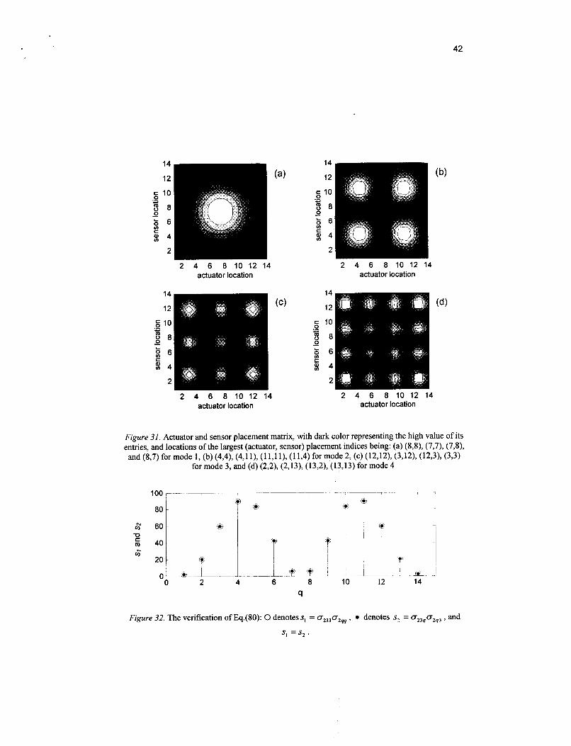
In this example n=4 and R=S=14. Using Eqs.(79) the placement matrices for the first four modes were determined and plotted in Figs.3 la-d. Before the placement procedure is applied the accuracy of Eq.(80) is checked. For this purpose the second mode is chosen, Le., i=2, and the following actuator and sensor locations are selected: j=k=3, l=m=q, and q=1, ..., 14. For these parameters Eq.(80) is as follows
q=l, . ..,14. The plots of the left- and right-hand side of the above equations are shown in Fig.32, showing good coincidence.
The maximal values of the actuator and sensor index in the placement matrix determine the preferred location of the actuator and sensor for each mode. Note that for each mode four locations - two sensor locations and two actuator locations - have the same maximal value. Moreover, they are symmetrical with respect to the beam center, see Fig.3 1. We selected four collocated sensors and actuators at the left-hand side of the beam center, one for each mode. Namely, for mode 1 - node 8, for mode 2 - node 4, for mode 3 - node 3, and for mode 4 - node 2.
7. Modal Actuators and Sensors
In some structural tests it is desirable to isolate (Le., excite and measure) a single mode. Such technique considerably simplifies the determination of modal parameters, see Ref.[ 131. This was first achieved by using the force appropriation method, called also the Asher method, see [ l l ] , or phase separation method, see 131. In this method a spatial distribution and the amplitudes of a harmonic input force are chosen to excite a single structural mode. Modal actuators or sensors were presented also in 141, [lo], and [SI with application to structural acoustic problems. This section follows Ref.[6].
42
2 4 6 8 10 12 14 actuator location
2 4 6 8 10 12 14 actuator location
2 4 6 8 10 12 14 actuator location
2 4 6 8 10 12 14 actuator location
Figure 31. Actuator and sensor placement matrix, with dark color representing the high value of its entries, and locations of the largest (actuator, sensor) placement indices being: (a) (8,8), (7,7), (7,8), and (8,7) for mode 1, (b) (4,4), (4,l I), (1 1,l l), (1 1,4) for mode 2, (c) (1 2,12), (3,12), (1 2,3), (3,3)
for mode 3, and (d) (2,2), (2,13), (13,2), (13,13) for mode 4
Figure 32. The verification of Eq.(80): 0 denotes s, = a2,,a2, , denotes s, = CT, ,~~ , , , , and s, = s2 .
43
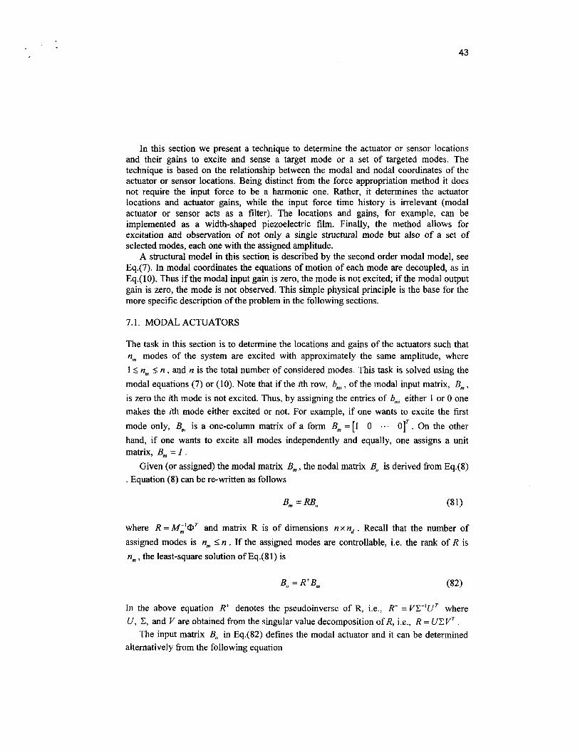
In this section we present a technique to determine the actuator or sensor locations and their gains to excite and sense a target mode or a set of targeted modes. The technique is based on the relationship between the modal and nodal coordinates of the actuator or sensor locations. Being distinct from the force appropriation method it does not require the input force to be a harmonic one. Rather, it determines the actuator locations and actuator gains, while the input force time history is irrelevant (modal actuator or sensor acts as a filter). The locations and gains, for example, can be implemented as a width-shaped piezoelectric film. Finally, the method allows for excitation and observation of not only a single structural mode but also of a set of selected modes, each one with the assigned amplitude.
A structural model in this section is described by the second order modal model, see Eq.(7). In modal coordinates the equations of motion of each mode are decoupled, as in Eq.( 10). Thus if the modal input gain is zero, the mode is not excited; if the modal output gain is zero, the mode is not observed. This simple physical principle is the base for the more specific description of the problem in the following sections.
7.1. MODAL ACTUATORS
The task in this section is to determine the locations and gains of the actuators such that nm modes of the system are excited with approximately the same amplitude, where 1 s n, I n , and n is the total number of considered modes. This task is solved using the modal equations (7) or (10). Note that if the ith row, b,, , of the modal input matrix, B, , is zero the ith mode is not excited. Thus, by assigning the entries of b,,,, either 1 or 0 one makes the ith mode either excited or not. For example, if one wants to excite the first mode only, B, is a one-column matrix of a form B, = [I 0 ... 01' . On the other hand, if one wants to excite all modes independently and equally, one assigns a unit matrix, B, = I .
Given (or assigned) the modal matrix B,,, , the nodal matrix Bo is derived fiom Eq.(8) . Equation (8) can be re-written as follows
where R = M;'cDT and matrix R is of dimensions n x nJ . Recall that the number of assigned modes is n, I n . If the assigned modes are controllable, i.e. the rank of R is n, , the least-square solution of Eq.(81) is
In the above equation R' denotes the pseudoinverse of R, i.e., R' = VC-'UT where U , C, and V are obtained from the singular value decomposition of R, Le., R = UCVT .
The input matrix Bo in Eq.(82) defines the modal actuator and it can be determined alternatively ftom the following equation
44
Bo = MOB, (83)
which does not require pseudoinverse and is equivalent to Eq.(81). Indeed, left- multiplication of Eq.(83) by Or gives @Bo = @*MOB,,, or OTBo = M,B,,,. Left- multiplication of the latter equation by Mi' results in Eq.(8 1).
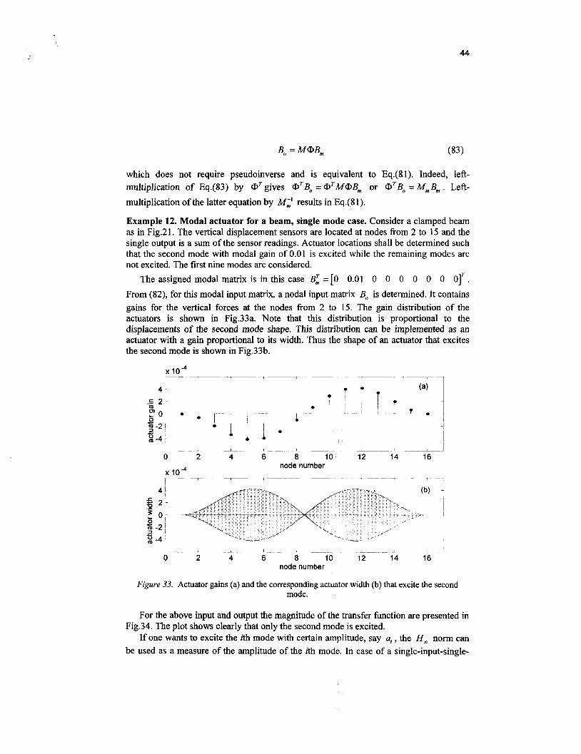
Example 12. Modal actuator for a beam, single mode case. Consider a clamped beam as in Fig.2 1. The vertical displacement sensors are located at nodes from 2 to 15 and the single output is a sum of the sensor readings. Actuator locations shall be determined such that the second mode with modal gain of 0.01 is excited while the remaining modes are not excited. The first nine modes are considered.
The assigned modal matrix is in this case B,' =[0 0.01 0 0 0 0 0 0 01' . From (82), for this modal input matrix, a nodal input matrix Bo is determined. It contains gains for the vertical forces at the nodes from 2 to 15. The gain distribution of the actuators is shown in Fig.33a. Note that this distribution is proportional to the displacements of the second mode shape. This distribution can be implemented as an actuator with a gain proportional to its width. Thus the shape of an actuator that excites the second mode is shown in Fig.33b.
4 .
I 7 I
1 7- 1
__
i 1
c
? I I.
T T
1
x I O " node number
- - _L ----I i--- - I -
0 2 4 6 8 10 12 14 16 node number
Figure 33. Actuator gains (a) and the corresponding actuator width (b) that excite the second mode.
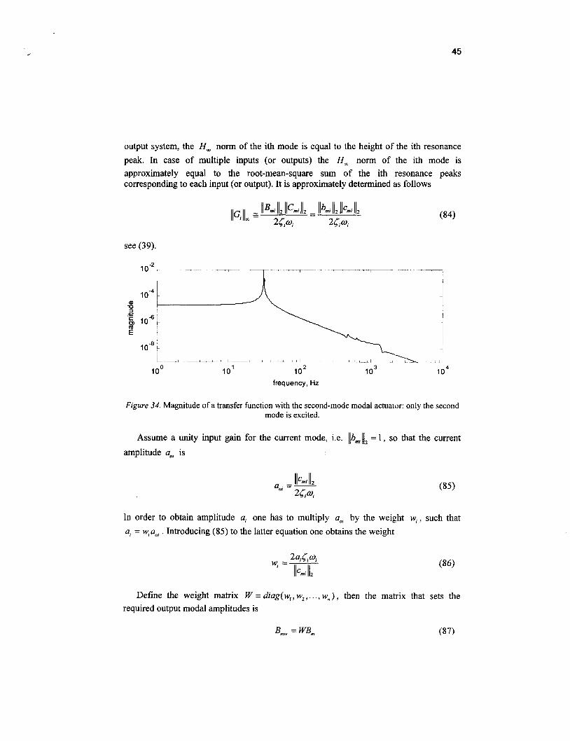
For the above input and output the magnitude of the transfer h c t i o n are presented in Fig.34. The plot shows clearly that only the second mode is excited.
If one wants to excite the ith mode with certain amplitude, say a,, the H , norm can be used as a measure of the amplitude of the ith mode. In case of a single-input-single-
, 45
output system, the Hm norm of the ith mode is equal to the height of the ith resonance peak. In case of multiple inputs (or outputs) the H, norm of the ith mode is approximately equal to the root-mean-square sum of the ith resonance peaks corresponding to each input (or output). It is approximately determined as follows
--.
frequency, Hz
Figure 34. Magnitude of a transfer function with the second-mode modal actuator: only the second mode is excited.
Assume a unity input gain for the current mode, i.e. llbml [Iz = 1, so that the current amplitude a,, is
In order to obtain amplitude a, one has to multiply a,,, by the weight w,, such that a, = w,a,, . Introducing ( 8 5 ) to the latter equation one obtains the weight
Define the weight matrix W = diag(w,, wz,. . ., w,,) , then the matrix that sets the required output modal amplitudes is
46
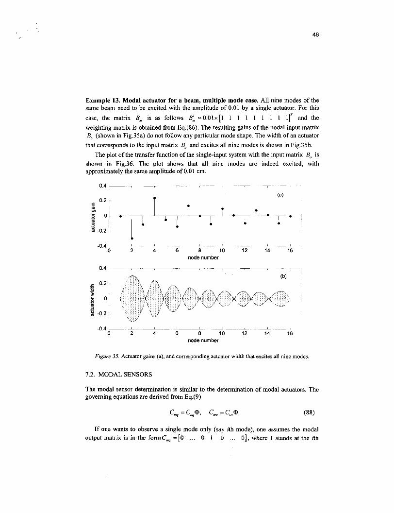
Example 13. Modal actuator for a beam, multiple mode case. All nine modes of the same beam need to be excited with the amplitude of 0.01 by a single actuator. For this case, the matrix B, is as follows B: =O.Olx[l 1 1 1 1 1 1 1 l]' and the weighting matrix is obtained from Eq.(86). The resulting gains of the nodal input matrix Bo (shown in Fig.35a) do not follow any particular mode shape. The width of an actuator that corresponds to the input matrix Bo and excites all nine modes is shown in Fig.35b.
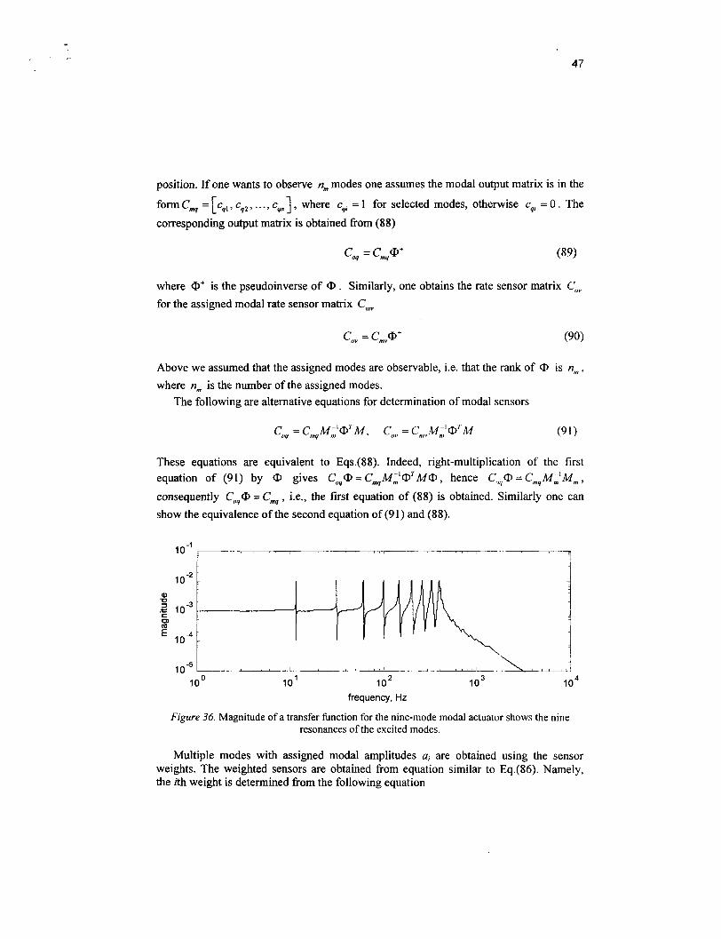
The plot of the transfer function of the single-input system with the input matrix Bo is shown in Fig.36. The plot shows that all nine modes are indeed excited, with approximately the same amplitude of 0.01 cm.
t
L i
I I I - 0 2 4 6 8 10 12 14 16
-0.4
node number
~- 0.4 -___ , 1-- , -__
Figure 35. Actuator gains (a), and corresponding actuator width that excites all nine modes.
7.2. MODAL SENSORS
The modal sensor determination is similar to the determination of modal actuators. The governing equations are derived from Eq.(9)
If one wants to observe a single mode only (say ith mode), one assumes the modal output matrix is in the form Cmq = [0 . . . 0 1 0 . . . 01, where 1 stands at the ith
47
position. If one wants to observe n,,, modes one assumes the modal output matrix is in the
form Cw = [ cq, , cq2 . . . , cqn ] where cq, = 1 for selected modes, otherwise cq, = 0 . The corresponding output matrix is obtained from (88)
where Q,+ is the pseudoinverse of Q, . Similarly, one obtains the rate sensor matrix C,,
for the assigned modal rate sensor matrix C,,,,
Above we assumed that the assigned modes are observable, i.e. that the rank of Q, is n,,, , where n,,, is the number of the assigned modes.
The following are alternative equations for determination of modal sensors
These equations are equivalent to Eqs.(88). Indeed, right-multiplication of the first equation of (91) by Q, gives Co,@ = C,,,qM;'OTMQ,, hence Coq@ = C,,,,M;'M,,
consequently Coq@ = C,,,,, , Le., the first equation of (88) is obtained. Similarly one can show the equivalence of the second equation of (91) and (88).
IO" 1 I I
l o o IO' IO2 i o 3 frequency, Hz
Figure 36. Magnitude of a transfer function for the nine-mode modal actuator shows the nine resonances of the excited modes.
Multiple modes with assigned modal amplitudes ai are obtained using the sensor weights. The weighted sensors are obtained from equation similar to Eq.(86). Namely, the ith weight is determined from the following equation
4%
where ai is the amplitude of the ith mode.
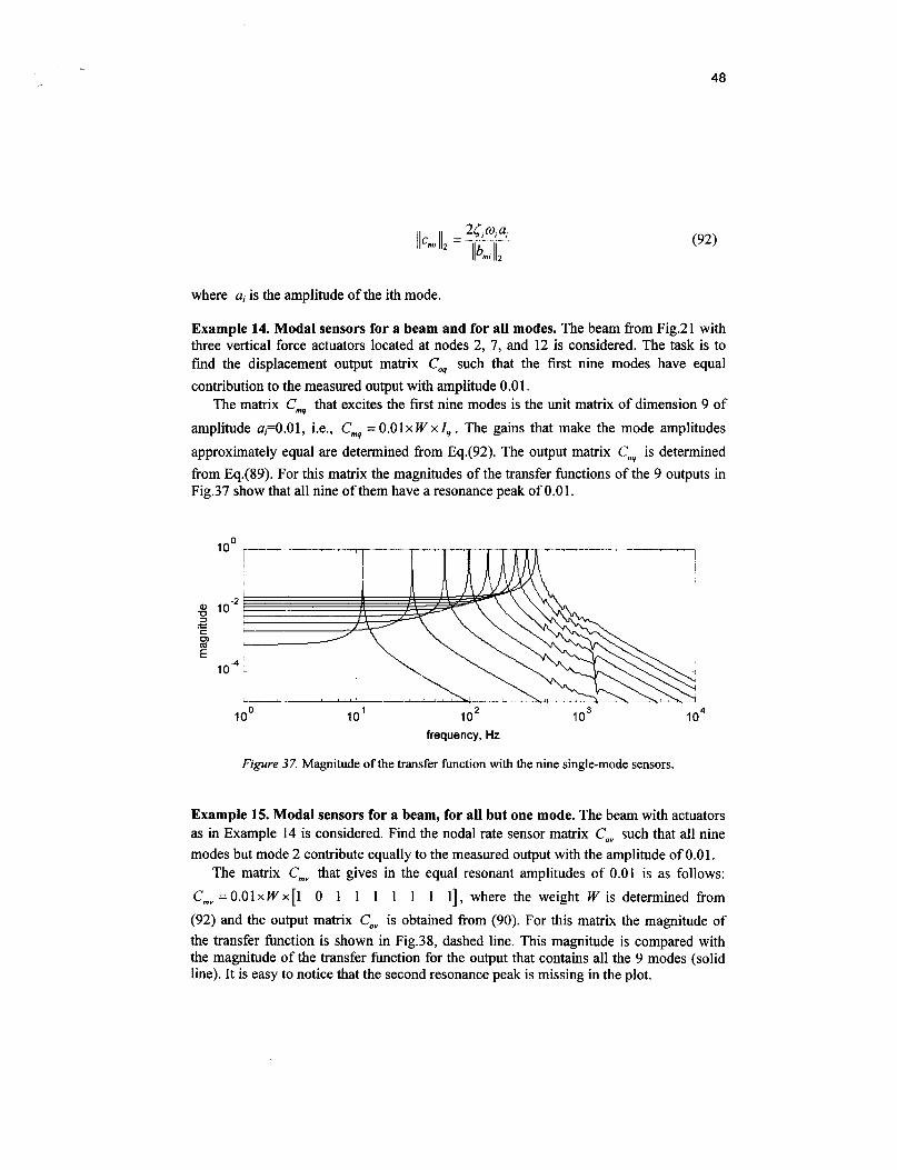
Example 14. Modal sensors for a beam and for all modes. The beam from Fig.21 with three vertical force actuators located at nodes 2, 7, and 12 is considered. The task is to find the displacement output matrix Co, such that the first nine modes have equal contribution to the measured output with amplitude 0.0 1.
The matrix Cmq that excites the first nine modes is the unit matrix of dimension 9 of amplitude u,=O.Ol, i.e., Cmq = 0 . 0 1 ~ W x l , . The gains that make the mode amplitudes approximately equal are determined from Eq.(92). The output matrix Coq is determined from Eq.(89). For this matrix the magnitudes of the transfer functions of the 9 outputs in Fig.37 show that all nine of them have a resonance peak of 0.01.
I O 0
@ lo-* s 8 c .- c
E I O 4
I O 0 I O ’ I O 2 i o 4 frequency, Hz
Figure 37. Magnitude of the transfer function with the nine single-mode sensors.
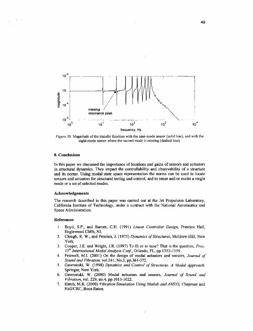
Example 15. Modal sensors for a beam, for all but one mode. The beam with actuators as in Example 14 is considered. Find the nodal rate sensor matrix C,, such that all nine modes but mode 2 contribute equally to the measured output with the amplitude of 0.0 1.
The matrix C,,,, that gives in the equal resonant amplitudes of 0.01 is as follows: C,,,, = O.OlxWx[l 0 1 1 1 1 1 1 11, where the weight W is determined from (92) and the output matrix C,, is obtained from (90). For this matrix the magnitude of the transfer function is shown in Fig.38, dashed line. This magnitude is compared with the magnitude of the transfer function for the output that contains all the 9 modes (solid line). It is easy to notice that the second resonance peak is missing in the plot.
49
resonance peak
L I 1 1 L 1 1
1 oo 10' IO2 1 o4 frequency, Hz
Fzgure 38 Magnitude of the transfer function with the nine-mode sensor (solid line), and with the eight-mode sensor where the second mode is missing (dashed line).
8. Conclusions
In this paper we discussed the importance of locations and gains of sensors and actuators in structural dynamics. They impact the controllability and observability of a structure and its norms. Using modal state space representation the norms can be used to locate sensors and actuators for structural testing and control, and to sense andior excite a single mode or a set of selected modes.
Acknowledgements The research described in this paper was carried out at the Jet Propulsion Laboratory, California Institute of Technology, under a contract with the National Aeronautics and Space Administration.
References 1.
2.
3.
4.
5.
6.
7.
Boyd, S.P., and Barratt, C.H. (1991) Linear Controller Design, Prentice Hall, Englewood Cliffs, NJ. Clough, R. W., and Penzien, J. (1975) Dynamics of Structures, McGraw-Hill, New York. Cooper, J.E. and Wright, J.R. (1997) To fit or to tune? That is the question, Proc. I f h International Modal Analysis Conf, Orlando, FL, pp.1353-1359. Friswell, M.I. (2001) On the design of modal actuators and sensors, Journal of Sound and Vibration, ~01.241, No.3, pp.361-372. Gawronski, W. (1998) Dynamics and Control of Structures. A Modal Approach. Springer, New York. Gawronski, W. (2000) Modal actuators and sensors, Journal of Sound and Vibration, vol. 229, no.4, pp.1013-1022. Hatch, M.R. (2000) Vibration Simulation Using Matlab and ANSYS, Chapman and HaWCRC, Boca Raton.
50
8. Hsu, C.-Y., Lin, C.-C. and Gaul, L., (1998) Vibration and sound radiation controls of beams using layered modal sensors and actuators, Smart Materials and Structures, vo1.7, pp.446-455.
9. Kailath, T. (1980) Linear Systems, Prentice Hall, Englewood Cliffs, NJ. 10. Lee, C.-K. and Moon, F.C. (1990) Modal sensorslactuators, J. of Applied
Mechanics, Trans. ASME, vol. 57, pp.434-44 1. 1 1. Maia, N.M.M., and Silva, J.M.M. (Eds.), (1997) Theoretical and Experimental
Modal Analysis, Research Studies Press Ltd., Taunton, England. 12. Moore, B.C. (1981) Principal component analysis in linear systems, controllability,
observability and model reduction, IEEE Trans. Autom. Control, vo1.26, pp. 17-32. 13. Phillips, A.W., and Allemang, R.J. (1996) Single degree-of-fieedom modal
parameter estimation methods. Proc. 1 4Ih International Modal Anabsis Con$, Deabom, MI, pp.253-260.
14. Preumont, A. (1997) Vibration Control of Active Structures, Kluwer Academic Publishers, Dordrecht.
15. Skogestad, S., and Postlethwaite, I. (1996) Multivariable Feedback Control, Wiley, Chichester, England.
16. Van de Wal, M., and de Jager, B. (2001) A review of methods for input/output selection, Automatica, ~01.37, pp.487-5 10.
17. Zhou, K., and Doyle, J.C. (1998) Essentials of Robust Control, Prentice Hall, Upper Saddle River, NJ.


