Embed Size (px)
Citation preview

Trigonometry Adapted from Precalculus by
Edition 2.1
David Lippman Melonie Rasmussen

ii
Copyright © 2018 David Lippman and Melonie Rasmussen
This text is licensed under a Creative Commons Attribution-Share Alike 3.0 United States License.
To view a copy of this license, visit http://creativecommons.org/licenses/by-sa/3.0/us/ or send a letter to Creative Commons, 171 Second Street, Suite 300, San Francisco, California, 94105, USA.
You are free: to Share — to copy, distribute, display, and perform the work to Remix — to make derivative works
Under the following conditions: Attribution. You must attribute the work in the manner specified by the author or licensor (but not in
any way that suggests that they endorse you or your use of the work). Share Alike. If you alter, transform, or build upon this work, you may distribute the resulting work
only under the same, similar or a compatible license.
With the understanding that: Waiver. Any of the above conditions can be waived if you get permission from the copyright holder. Other Rights. In no way are any of the following rights affected by the license:
• Your fair dealing or fair use rights;• Apart from the remix rights granted under this license, the author's moral rights;• Rights other persons may have either in the work itself or in how the work is used, such as
publicity or privacy rights.• Notice — For any reuse or distribution, you must make clear to others the license terms of
this work. The best way to do this is with a link to this web page:http://creativecommons.org/licenses/by-sa/3.0/us/
In addition to these rights, we give explicit permission to remix small portions of this book (less than 10% cumulative) into works that are CC-BY, CC-BY-SA-NC, or GFDL licensed.
Selected exercises were remixed from Precalculus by D.H. Collingwood and K.D. Prince, originally licensed under the GNU Free Document License, with permission from the authors. These are marked in the book as [UW].
Portions of chapter 3 were remixed from College Algebra by Carl Stitz and Jeff Zeager, originally licensed under a Creative Commons Attribution ShareAlike Non-Commercial license, used with permission from the authors.
Portions of chapter 9 were remixed from work by Lara Michaels, and contains content remixed from Precalculus by OpenStax, originally licensed under a Creative Commons Attribution license. The original version is available online for free at OpenStax.org.
Cover photos by Ralph Morasch and David Lippman, of artwork by John Rogers. Lituus, 2010. Dichromatic glass and aluminum. Washington State Arts Commission in partnership with Pierce College

i
About the Authors
David Lippman received his master’s degree in mathematics from Western Washington University and has been teaching at Pierce College since Fall 2000. Melonie Rasmussen also received her master’s degree in mathematics from Western Washington University and has been teaching at Pierce College since Fall 2002. Prior to this Melonie taught for the
Puyallup School district for 6 years after receiving her teaching credentials from Pacific Lutheran University. We have both been long time advocates of open learning, open materials, and basically any idea that will reduce the cost of education for students. It started by supporting the college’s calculator rental program, and running a book loan scholarship program. Eventually the frustration with the escalating costs of commercial text books and the online homework systems that charged for access led them to take action. First, David developed IMathAS, open source online math homework software that runs WAMAP.org and MyOpenMath.com. Through this platform, we became integral parts of a vibrant sharing and learning community of teachers from around Washington State that support and contribute to WAMAP. Our pioneering efforts, supported by dozens of other dedicated faculty and financial support from the WA-SBCTC, have led to a system used by thousands of students every quarter, saving hundreds of thousands of dollars over comparable commercial offerings. David continued further and wrote his first open textbook, Math in Society, a math for liberal arts majors book, after being frustrated by students having to pay $100+ for a textbook for a terminal course. Together, frustrated by both cost and the style of commercial texts, we began writing PreCalculus: An Investigation of Functions in 2010. Since then, David has contributed to several other open texts.

ii
Acknowledgements We would like to thank the following for their generous support and feedback.
• The community of WAMAP users and developers for creating a majority of the homework content used in our online homework sets.
• Pierce College students in our Fall 2010 - Summer 2011 Math 141 and Math 142 classes for helping correct typos, identifying videos related to the homework, and being our willing test subjects.
• The Open Course Library Project for providing the support needed to produce a full course package for these courses.
• Mike Kenyon, Chris Willett, Tophe Anderson, and Vauhn Foster-Grahler for reviewing the course and giving feedback and suggestions.
• Our Pierce College colleagues for providing their suggestions.
• Tophe Anderson, James Gray, and Lawrence Morales for their feedback and suggestions in content and examples.
• Jeff Eldridge for extensive proofreading and suggestions for clarification.
• James Sousa for developing videos associated with the online homework.
• Kevin Dimond for his work on indexing the book and creating PowerPoint slides.
• Faculty at Green River Community College and the Maricopa College District for their feedback and suggestions.
• Lara Michaels for contributing the basis for a conics chapter.
• The dozens of instructors who have sent us typos or suggestions over the years.

iii
Preface Over the years, when reviewing books we found that many had been mainstreamed by the publishers in an effort to appeal to everyone, leaving them with very little character. There were only a handful of books that had the conceptual and application driven focus we liked, and most of those were lacking in other aspects we cared about, like providing students sufficient examples and practice of basic skills. The largest frustration, however, was the never ending escalation of cost and being forced into new editions every three years. We began researching open textbooks, however the ability for those books to be adapted, remixed, or printed were often limited by the types of licenses, or didn’t approach the material the way we wanted. This book is available online for free, in both Word and PDF format. You are free to change the wording, add materials and sections or take them away. We welcome feedback, comments and suggestions for future development at [email protected]. Additionally, if you add a section, chapter or problems, we would love to hear from you and possibly add your materials so everyone can benefit. In writing this book, our focus was on the story of functions. We begin with function notation, a basic toolkit of functions, and the basic operation with functions: composition and transformation. Building from these basic functions, as each new family of functions is introduced we explore the important features of the function: its graph, domain and range, intercepts, and asymptotes. The exploration then moves to evaluating and solving equations involving the function, finding inverses, and culminates with modeling using the function. The "rule of four" is integrated throughout - looking at the functions verbally, graphically, numerically, as well as algebraically. We feel that using the “rule of four” gives students the tools they need to approach new problems from various angles. Often the “story problems of life” do not always come packaged in a neat equation. Being able to think critically, see the parts and build a table or graph a trend, helps us change the words into meaningful and measurable functions that model the world around us. There is nothing we hate more than a chapter on exponential equations that begins "Exponential functions are functions that have the form f(x)=ax." As each family of functions is introduced, we motivate the topic by looking at how the function arises from life scenarios or from modeling. Also, we feel it is important that precalculus be the bridge in level of thinking between algebra and calculus. In algebra, it is common to see numerous examples with very similar homework exercises, encouraging the student to mimic the examples. Precalculus provides a link that takes students from the basic plug & chug of formulaic calculations towards building an understanding that equations and formulas have deeper meaning and purpose. While you will find examples and similar exercises for the basic skills in this book, you will also find examples of multistep problem solving along with exercises in multistep problem solving. Often times these exercises will not exactly mimic the exercises, forcing the students to employ their critical thinking skills and apply the skills they've learned to new situations. By

iv
developing students’ critical thinking and problem solving skills this course prepares students for the rigors of Calculus. While we followed a fairly standard ordering of material in the first half of the book, we took some liberties in the trig portion of the book. It is our opinion that there is no need to separate unit circle trig from triangle trig, and instead integrated them in the first chapter. Identities are introduced in the first chapter, and revisited throughout. Likewise, solving is introduced in the second chapter and revisited more extensively in the third chapter. As with the first part of the book, an emphasis is placed on motivating the concepts and on modeling and interpretation.
About the Second Edition About 4 years and several minor typo revisions after the original release of this book, we started contemplating creating a second edition. We didn’t want to change much; we’ve always found it very annoying when new editions change things just for the sake of making it seem different. However, in talking with instructors from around the country, we knew there were a few topics that we had left out that other schools need. We didn’t want to suffer the same “content bloat” that many commercial books do, but we also wanted to make it easier for more schools to adopt open resources. We put our plans for a new revision on hold after OpenStax started working on a precalculus book, using the first edition of this text as a base. After the final product came out, though, we felt it had strayed a bit far from our original vision. We had written this text, not to be an encyclopedic reference text, but to be a concise, easy-to-read, student-friendly approach to precalculus. We valued contextual motivation and conceptual understanding over procedural skills. Our book took, in places, a non-traditional approach to topics and content ordering. Ultimately, we decided to go ahead with this second edition. The primary changes in the second edition are:
• New, higher resolution graphs throughout • New sections added to Chapter 3:
o 3.4 Factor theorem (includes long division of polynomials) o 3.5 Real zeros of polynomials (using rational roots theorem) o 3.6 Complex zeros of polynomials
• Coverage of oblique asymptotes added to the rational equations section (now 3.7) • A new section 8.5 on dot product of vectors • A new chapter 9 on conic sections
There were many additional refinements, some new examples added, and Try it Now answers expanded, but most of the book remains unchanged.

v
Instructor Resources As part of the Washington Open Course Library project, we developed a full course package to accompany this text. The course shell was built for the IMathAS online homework platform, and is available for Washington State faculty at www.wamap.org and mirrored for others at www.myopenmath.com. It contains:
• Online homework for each section (algorithmically generated, free response), most with video help associated.
• Video lessons for each section. The videos were mostly created and selected by James Sousa, of Mathispower4u.
• A selection of printable class worksheets, activities, and handouts • Support materials for an example course (does not include all sections):
o Suggested syllabus and Day by day course guide o Instructor guide with lecture outlines and examples o Discussion forums o Diagnostic review o Chapter review problems o Sample quizzes and sample chapter exams
The course shell was designed to follow Quality Matters (QM) guidelines, but has not yet been formally reviewed. Getting Started To get started using this textbook and the online supplementary materials,
• Request an instructor account on WAMAP (in Washington) or MyOpenMath (outside Washington).
• Review the table of contents of the text, and compare it to your course outcomes or student learning objectives. Determine which sections you will need to cover, and which to omit. If there are topics in your outcomes that are not in the text, explore other sources like the Stitz/Zeager Precalc or OpenStax Precalc to supplement from. Also check the book’s website, as we may offer additional online-only topics.
• Once your instructor account is approved, log in, and click Add New Course • From the “Use content from a template course”, select “Precalculus –
Lippman/Rasmussen 2nd Ed”. Note that you might also see two half-book templates, one covering chapters 1 – 4, and the other covering chapters 5 – 9.
• Once you have copied the course, go through and remove any sections you don’t need for your course. Refer to the Training Course Quickstart videos in MyOpenMath and WAMAP for more details on how to make those changes.

vi
How To Be Successful In This Course This is not a high school math course, although for some of you the content may seem familiar. There are key differences to what you will learn here, how quickly you will be required to learn it and how much work will be required of you. You will no longer be shown a technique and be asked to mimic it repetitively as the only way to prove learning. Not only will you be required to master the technique, but you will also be required to extend that knowledge to new situations and build bridges between the material at hand and the next topic, making the course highly cumulative. As a rule of thumb, for each hour you spend in class, you should expect this course will require an average of 2 hours of out-of-class focused study. This means that some of you with a stronger background in mathematics may take less, but if you have a weaker background or any math anxiety it will take you more. Notice how this is the equivalent of having a part time job, and if you are taking a fulltime load of courses as many college students do, this equates to more than a full time job. If you must work, raise a family and take a full load of courses all at the same time, we recommend that you get a head start & get organized as soon as possible. We also recommend that you spread out your learning into daily chunks and avoid trying to cram or learn material quickly before an exam. To be prepared, read through the material before it is covered in class and note or highlight the material that is new or confusing. The instructor’s lecture and activities should not be the first exposure to the material. As you read, test your understanding with the Try it Now problems in the book. If you can’t figure one out, try again after class, and ask for help if you still can’t get it. As soon as possible after the class session recap the day’s lecture or activities into a meaningful format to provide a third exposure to the material. You could summarize your notes into a list of key points, or reread your notes and try to work examples done in class without referring back to your notes. Next, begin any assigned homework. The next day, if the instructor provides the opportunity to clarify topics or ask questions, do not be afraid to ask. If you are afraid to ask, then you are not getting your money’s worth! If the instructor does not provide this opportunity, be prepared to go to a tutoring center or build a peer study group. Put in quality effort and time and you can get quality results. Lastly, if you feel like you do not understand a topic. Don’t wait, ASK FOR HELP! ASK: Ask a teacher or tutor, Search for ancillaries, Keep a detailed list of questions FOR: Find additional resources, Organize the material, Research other learning options HELP: Have a support network, Examine your weaknesses, List specific examples & Practice Best of luck learning! We hope you like the course & love the price. David & Melonie

vii
Table of Contents
About the Authors ............................................................................................................ i Acknowledgements ......................................................................................................... ii Preface ........................................................................................................................... iii About the Second Edition .............................................................................................. iv Instructor Resources ...................................................... Error! Bookmark not defined. How To Be Successful In This Course .......................................................................... vi Table of Contents .......................................................................................................... vii
Chapter 1: Functions ........................................................................................................ 1
Section 1.1 Functions and Function Notation ................................................................. 1 Section 1.2 Domain and Range ..................................................................................... 22 Section 1.3 Rates of Change and Behavior of Graphs .................................................. 36 Section 1.4 Composition of Functions .......................................................................... 51 Section 1.5 Transformation of Functions ..................................................................... 64 Section 1.6 Inverse Functions ....................................................................................... 93
Chapter 2: Linear Functions........................................................................................ 101 Section 2.1 Linear Functions ...................................................................................... 101 Section 2.2 Graphs of Linear Functions ..................................................................... 114 Section 2.3 Modeling with Linear Functions .............................................................. 129 Section 2.4 Fitting Linear Models to Data .................................................................. 141 Section 2.5 Absolute Value Functions ........................................................................ 140
Chapter 3: Polynomial and Rational Functions ......................................................... 159 Section 3.1 Power Functions & Polynomial Functions .............................................. 159 Section 3.2 Quadratic Functions ................................................................................. 167 Section 3.3 Graphs of Polynomial Functions ............................................................. 181 Section 3.4 Factor Theorem and Remainder Theorem ............................................... 194 Section 3.5 Real Zeros of Polynomials ....................................................................... 203 Section 3.6 Complex Zeros ......................................................................................... 210 Section 3.7 Rational Functions ................................................................................... 218 Section 3.8 Inverses and Radical Functions ............................................................... 239
Chapter 4: Exponential and Logarithmic Functions ................................................. 249 Section 4.1 Exponential Functions ............................................................................. 249 Section 4.2 Graphs of Exponential Functions ............................................................ 267 Section 4.3 Logarithmic Functions ............................................................................. 277 Section 4.4 Logarithmic Properties ............................................................................ 289 Section 4.5 Graphs of Logarithmic Functions ............................................................ 300 Section 4.6 Exponential and Logarithmic Models ...................................................... 308 Section 4.7 Fitting Exponential Models to Data ......................................................... 328

viii
Chapter 5: Trigonometric Functions of Angles ......................................................... 337 Section 5.1 Circles ...................................................................................................... 337 Section 5.2 Angles ...................................................................................................... 347 Section 5.3 Points on Circles Using Sine and Cosine ................................................. 362 Section 5.4 The Other Trigonometric Functions ........................................................ 375 Section 5.5 Right Triangle Trigonometry ................................................................... 385
Chapter 6: Periodic Functions ..................................................................................... 395 Section 6.1 Sinusoidal Graphs .................................................................................... 395 Section 6.2 Graphs of the Other Trig Functions ......................................................... 412 Section 6.3 Inverse Trig Functions ............................................................................. 422 Section 6.4 Solving Trig Equations ............................................................................ 430 Section 6.5 Modeling with Trigonometric Functions ................................................. 441
Chapter 7: Trigonometric Equations and Identities ................................................. 453 Section 7.1 Solving Trigonometric Equations with Identities .................................... 453 Section 7.2 Addition and Subtraction Identities ......................................................... 461 Section 7.3 Double Angle Identities ........................................................................... 477 Section 7.4 Modeling Changing Amplitude and Midline ........................................... 495
Chapter 8: Further Applications of Trigonometry.................................................... 497 Section 8.1 Non-Right Triangles: Laws of Sines and Cosines ................................... 497 Section 8.2 Polar Coordinates ..................................................................................... 514 Section 8.3 Polar Form of Complex Numbers ............................................................ 528 Section 8.4 Vectors ..................................................................................................... 541 Section 8.5 Dot Product .............................................................................................. 555 Section 8.6 Parametric Equations ............................................................................... 564
Chapter 9: Conics ......................................................................................................... 579 Section 9.1 Ellipses ..................................................................................................... 579 Section 9.2 Hyperbolas ............................................................................................... 597 Section 9.3 Parabolas and Non-Linear Systems ......................................................... 617 Section 9.4 Conics in Polar Coordinates .................................................................... 630
Answers to Selected Exercises...................................................................................... 641 Index ............................................................................................................................... 691

This chapter is part of Precalculus: An Investigation of Functions © Lippman & Rasmussen 2017. This material is licensed under a Creative Commons CC-BY-SA license.
Chapter 5: Trigonometric Functions of Angles In the previous chapters, we have explored a variety of functions which could be combined to form a variety of shapes. In this discussion, one common shape has been missing: the circle. We already know certain things about the circle, like how to find area and circumference, and the relationship between radius and diameter, but now, in this chapter, we explore the circle and its unique features that lead us into the rich world of trigonometry.
Section 5.1 Circles ...................................................................................................... 337 Section 5.2 Angles ...................................................................................................... 347 Section 5.3 Points on Circles using Sine and Cosine.................................................. 362 Section 5.4 The Other Trigonometric Functions ........................................................ 375 Section 5.5 Right Triangle Trigonometry ................................................................... 385
Section 5.1 Circles To begin, we need to find distances. Starting with the Pythagorean Theorem, which relates the sides of a right triangle, we can find the distance between two points.
Pythagorean Theorem The Pythagorean Theorem states that the sum of the squares of the legs of a right triangle will equal the square of the hypotenuse of the triangle. In graphical form, given the triangle shown, 2 2 2a b c+ = .
We can use the Pythagorean Theorem to find the distance between two points on a graph. Example 1
Find the distance between the points (-3, 2) and (2, 5). By plotting these points on the plane, we can then draw a right triangle with these points at each end of the hypotenuse. We can calculate horizontal width of the triangle to be 5 and the vertical height to be 3.
a
b
c

338 Chapter 5
From these we can find the distance between the points using the Pythagorean Theorem:
34
3435 222
=
=+=
dist
dist
Notice that the width of the triangle was calculated using the difference between the x (input) values of the two points, and the height of the triangle was found using the difference between the y (output) values of the two points. Generalizing this process gives us the distance formula.
Distance Formula The distance between two points ),( 11 yx and ),( 22 yx can be calculated as
212
212 )()( yyxxdist −+−=
Try it Now 1. Find the distance between the points (1, 6) and (3, -5). Circles If we wanted to find an equation to represent a circle with a radius of r centered at a point (h, k), we notice that the distance between any point (x, y) on the circle and the center point is always the same: r. Noting this, we can use our distance formula to write an equation for the radius:
22 )()( kyhxr −+−= Squaring both sides of the equation gives us the standard equation for a circle.
Equation of a Circle The equation of a circle centered at the point (h, k) with radius r can be written as
222 )()( rkyhx =−+− Notice that a circle does not pass the vertical line test. It is not possible to write y as a function of x or vice versa.
r
(h, k)
(x, y)

Section 5.1 Circles 339
Example 2 Write an equation for a circle centered at the point (-3, 2) with radius 4. Using the equation from above, h = -3, k = 2, and the radius r = 4. Using these in our formula,
222 4)2())3(( =−+−− yx simplified, this gives 16)2()3( 22 =−++ yx
Example 3
Write an equation for the circle graphed here. This circle is centered at the origin, the point (0, 0). By measuring horizontally or vertically from the center out to the circle, we can see the radius is 3. Using this information in our formula gives:
222 3)0()0( =−+− yx simplified, this gives 922 =+ yx
Try it Now 2. Write an equation for a circle centered at (4, -2) with radius 6. Notice that, relative to a circle centered at the origin, horizontal and vertical shifts of the circle are revealed in the values of h and k, which are the coordinates for the center of the circle. Points on a Circle As noted earlier, an equation for a circle cannot be written so that y is a function of x or vice versa. To find coordinates on the circle given only the x or y value, we must solve algebraically for the unknown values. Example 4
Find the points on a circle of radius 5 centered at the origin with an x value of 3. We begin by writing an equation for the circle centered at the origin with a radius of 5.
2522 =+ yx Substituting in the desired x value of 3 gives an equation we can solve for y.

340 Chapter 5
416
16925253
2
22
±=±=
=−=
=+
y
yy
There are two points on the circle with an x value of 3: (3, 4) and (3, -4).
Example 5
Find the x intercepts of a circle with radius 6 centered at the point (2, 4). We can start by writing an equation for the circle.
36)4()2( 22 =−+− yx To find the x intercepts, we need to find the points where y = 0. Substituting in zero for y, we can solve for x.
36)40()2( 22 =−+−x 3616)2( 2 =+−x
20)2( 2 =−x 202 ±=−x
522202 ±=±=x The x intercepts of the circle are ( )0,522 + and ( )0,522 −
Example 6
In a town, Main Street runs east to west, and Meridian Road runs north to south. A pizza store is located on Meridian 2 miles south of the intersection of Main and Meridian. If the store advertises that it delivers within a 3-mile radius, how much of Main Street do they deliver to? This type of question is one in which introducing a coordinate system and drawing a picture can help us solve the problem. We could either place the origin at the intersection of the two streets, or place the origin at the pizza store itself. It is often easier to work with circles centered at the origin, so we’ll place the origin at the pizza store, though either approach would work fine. Placing the origin at the pizza store, the delivery area with radius 3 miles can be described as the region inside the circle described by 922 =+ yx . Main Street, located 2 miles north of the pizza store and running east to west, can be described by the equation y = 2.

Section 5.1 Circles 341
To find the portion of Main Street the store will deliver to, we first find the boundary of their delivery region by looking for where the delivery circle intersects Main Street. To find the intersection, we look for the points on the circle where y = 2. Substituting y = 2 into the circle equation lets us solve for the corresponding x values.
236.25
54992
2
22
±≈±=
=−=
=+
x
xx
This means the pizza store will deliver 2.236 miles down Main Street east of Meridian and 2.236 miles down Main Street west of Meridian. We can conclude that the pizza store delivers to a 4.472 mile long segment of Main St.
In addition to finding where a vertical or horizontal line intersects the circle, we can also find where an arbitrary line intersects a circle. Example 7
Find where the line xxf 4)( = intersects the circle 16)2( 22 =+− yx . Normally, to find an intersection of two functions f(x) and g(x) we would solve for the x value that would make the functions equal by solving the equation f(x) = g(x). In the case of a circle, it isn’t possible to represent the equation as a function, but we can utilize the same idea. The output value of the line determines the y value: xxfy 4)( == . We want the y value of the circle to equal the y value of the line, which is the output value of the function. To do this, we can substitute the expression for y from the line into the circle equation.
16)2( 22 =+− yx replace y with the line formula: xy 4= 16)4()2( 22 =+− xx expand
161644 22 =++− xxx simplify 164417 2 =+− xx since this equation is quadratic, we arrange one side to be 0 012417 2 =−− xx
Since this quadratic doesn’t appear to be easily factorable, we can use the quadratic formula to solve for x:
348324
)17(2)12)(17(4)4()4( 2 ±=
−−−±−−=x , or approximately x ≈ 0.966 or -0.731
From these x values we can use either equation to find the corresponding y values.

342 Chapter 5
Since the line equation is easier to evaluate, we might choose to use it:
923.2)731.0(4)731.0(864.3)966.0(4)966.0(−=−=−=
===fyfy
The line intersects the circle at the points (0.966, 3.864) and (-0.731, -2.923).
Try it Now 3. A small radio transmitter broadcasts in a 50 mile radius. If you drive along a straight
line from a city 60 miles north of the transmitter to a second city 70 miles east of the transmitter, during how much of the drive will you pick up a signal from the transmitter?
Important Topics of This Section Distance formula Equation of a Circle Finding the x coordinate of a point on the circle given the y coordinate or vice versa Finding the intersection of a circle and a line
Try it Now Answers 1. 55 2. 36)2()4( 22 =++− yx 3. The circle can be represented by 222 50=+ yx .
Finding a line from (0,60) to (70,0) gives xy706060 −= .
Substituting the line equation into the circle gives 2
2 26060 5070
x x + − =
.
Solving this equation, we find x = 14 or x = 45.29, corresponding to points (14, 48) and (45.29, 21.18). The distance between these points is 41.21 miles.

Section 5.1 Circles 343
Section 5.1 Exercises
1. Find the distance between the points (5,3) and (-1,-5).
2. Find the distance between the points (3,3) and (-3,-2).
3. Write an equation of the circle centered at (8 , -10) with radius 8.
4. Write an equation of the circle centered at (-9, 9) with radius 16.
5. Write an equation of the circle centered at (7, -2) that passes through (-10, 0).
6. Write an equation of the circle centered at (3, -7) that passes through (15, 13).
7. Write an equation for a circle where the points (2, 6) and (8, 10) lie along a diameter.
8. Write an equation for a circle where the points (-3, 3) and (5, 7) lie along a diameter.
9. Sketch a graph of ( ) ( )2 22 3 9x y− + + = .
10. Sketch a graph of ( ) ( )2 21 2 1 6x y+ + − = .
11. Find the y intercept(s) of the circle with center (2, 3) with radius 3.
12. Find the x intercept(s) of the circle with center (2, 3) with radius 4.
13. At what point in the first quadrant does the line with equation 2 5y x= + intersect a circle with radius 3 and center (0, 5)?
14. At what point in the first quadrant does the line with equation 2y x= + intersect the circle with radius 6 and center (0, 2)?
15. At what point in the second quadrant does the line with equation 2 5y x= + intersect a circle with radius 3 and center (-2, 0)?
16. At what point in the first quadrant does the line with equation 2y x= + intersect the circle with radius 6 and center (-1,0)?
17. A small radio transmitter broadcasts in a 53 mile radius. If you drive along a straight line from a city 70 miles north of the transmitter to a second city 74 miles east of the transmitter, during how much of the drive will you pick up a signal from the transmitter?
18. A small radio transmitter broadcasts in a 44 mile radius. If you drive along a straight
line from a city 56 miles south of the transmitter to a second city 53 miles west of the transmitter, during how much of the drive will you pick up a signal from the transmitter?

344 Chapter 5
19. A tunnel connecting two portions of a space
station has a circular cross-section of radius 15 feet. Two walkway decks are constructed in the tunnel. Deck A is along a horizontal diameter and another parallel Deck B is 2 feet below Deck A. Because the space station is in a weightless environment, you can walk vertically upright along Deck A, or vertically upside down along Deck B. You have been assigned to paint “safety stripes” on each deck level, so that a 6 foot person can safely walk upright along either deck. Determine the width of the “safe walk zone” on each deck. [UW]
20. A crawling tractor sprinkler is
located as pictured here, 100 feet south of a sidewalk. Once the water is turned on, the sprinkler waters a circular disc of radius 20 feet and moves north along the hose at the rate of ½ inch/second. The hose is perpendicular to the 10 ft. wide sidewalk. Assume there is grass on both sides of the sidewalk. [UW]
a) Impose a coordinate system.
Describe the initial coordinates of the sprinkler and find equations of the lines forming and find equations of the lines forming the north and south boundaries of the sidewalk.
b) When will the water first strike the sidewalk? c) When will the water from the sprinkler fall completely north of the sidewalk? d) Find the total amount of time water from the sprinkler falls on the sidewalk. e) Sketch a picture of the situation after 33 minutes. Draw an accurate picture of the
watered portion of the sidewalk. f) Find the area of grass watered after one hour.

Section 5.1 Circles 345
21. Erik’s disabled sailboat is floating anchored 3 miles East and 2 miles north of Kingsford. A ferry leaves Kingsford heading toward Eaglerock at 12 mph. Eaglerock is 6 miles due east of Kingsford. After 20 minutes the ferry turns, heading due south. Bander is 8 miles south and 1 mile west of Eaglerock. Impose coordinates with Bander as the origin. [UW]
a) Find equations for the lines along which the ferry is moving and draw in these
lines. b) The sailboat has a radar scope that will detect any object within 3 miles of the
sailboat. Looking down from above, as in the picture, the radar region looks like a circular disk. The boundary is the “edge” or circle around this disk, the interior is everything inside of the circle, and the exterior is everything outside of the circle. Give the mathematical description (an equation or inequality) of the boundary, interior and exterior of the radar zone. Sketch an accurate picture of the radar zone by determining where the line connecting Kingsford and Eaglerock would cross the radar zone.
c) When does the ferry enter the radar zone? d) Where and when does the ferry exit the radar zone? e) How long does the ferry spend inside the radar zone?
North
Kingsford Eaglerock
Bander

346 Chapter 5
22. Nora spends part of her summer driving a combine during the wheat harvest. Assume she starts at the indicated position heading east at 10 ft/sec toward a circular wheat field of radius 200 ft. The combine cuts a swath 20 feet wide and begins when the corner of the machine labeled “a” is 60 feet north and 60 feet west of the western-most edge of the field. [UW]
a) When does Nora’s combine first start cutting the wheat? b) When does Nora’s combine first start cutting a swath 20 feet wide? c) Find the total amount of time wheat is being cut during this pass across the field. d) Estimate the area of the swath cut during this pass across the field.
23. The vertical cross-section of a drainage ditch is
pictured to the right. Here, R indicates in each case the radius of a circle with R = 10 feet, where all of the indicated circle centers lie along a horizontal line 10 feet above and parallel to the ditch bottom. Assume that water is flowing into the ditch so that the level above the bottom is rising at a rate of 2 inches per minute. [UW]
a) When will the ditch be completely full? b) Find a piecewise defined function that
models the vertical cross-section of the ditch. c) What is the width of the filled portion of the ditch after 1 hour and 18 minutes? d) When will the filled portion of the ditch be 42 feet wide? 50 feet wide? 73 feet
wide?

Section 5.2 Angles 347
Section 5.2 Angles Because many applications involving circles also involve a rotation of the circle, it is natural to introduce a measure for the rotation, or angle, between two rays (line segments) emanating from the center of a circle. The angle measurement you are most likely familiar with is degrees, so we’ll begin there.
Measure of an Angle The measure of an angle is a measurement between two intersecting lines, line segments or rays, starting at the initial side and ending at the terminal side. It is a rotational measure, not a linear measure.
Measuring Angles
Degrees A degree is a measurement of angle. One full rotation around the circle is equal to 360 degrees, so one degree is 1/360 of a circle. An angle measured in degrees should always include the unit “degrees” after the number, or include the degree symbol °. For example, 90 degrees = °90 .
Standard Position When measuring angles on a circle, unless otherwise directed, we measure angles in standard position: starting at the positive horizontal axis and with counter-clockwise rotation.
Example 1
Give the degree measure of the angle shown on the circle. The vertical and horizontal lines divide the circle into quarters. Since one full rotation is 360 degrees= °360 , each quarter rotation is 360/4 = °90 or 90 degrees.
Example 2
Show an angle of °30 on the circle. An angle of °30 is 1/3 of °90 , so by dividing a quarter rotation into thirds, we can sketch a line at °30 .
initial side
terminal side
angle

348 Chapter 5
Going Greek When representing angles using variables, it is traditional to use Greek letters. Here is a list of commonly encountered Greek letters.
θ ϕ or φ α β γ theta phi alpha beta gamma
Working with Angles in Degrees Notice that since there are 360 degrees in one rotation, an angle greater than 360 degrees would indicate more than 1 full rotation. Shown on a circle, the resulting direction in which this angle’s terminal side points would be the same as for another angle between 0 and 360 degrees. These angles would be called coterminal.
Coterminal Angles After completing their full rotation based on the given angle, two angles are coterminal if they terminate in the same position, so their terminal sides coincide (point in the same direction).
Example 3
Find an angle θ that is coterminal with °800 , where 0 360θ° ≤ < ° Since adding or subtracting a full rotation, 360 degrees, would result in an angle with terminal side pointing in the same direction, we can find coterminal angles by adding or subtracting 360 degrees. An angle of 800 degrees is coterminal with an angle of 800-360 = 440 degrees. It would also be coterminal with an angle of 440-360 = 80 degrees. The angle °= 80θ is coterminal with °800 . By finding the coterminal angle between 0 and 360 degrees, it can be easier to see which direction the terminal side of an angle points in.
Try it Now 1. Find an angle α that is coterminal with °870 , where °<≤° 3600 α .

Section 5.2 Angles 349
On a number line a positive number is measured to the right and a negative number is measured in the opposite direction (to the left). Similarly a positive angle is measured counterclockwise and a negative angle is measured in the opposite direction (clockwise). Example 4
Show the angle °− 45 on the circle and find a positive angleα that is coterminal and °<≤° 3600 α .
Since 45 degrees is half of 90 degrees, we can start at the positive horizontal axis and measure clockwise half of a 90 degree angle. Since we can find coterminal angles by adding or subtracting a full rotation of 360 degrees, we can find a positive coterminal angle here by adding 360 degrees:
°=°+°− 31536045 Try it Now 2. Find an angle β coterminal with 300− ° where 0 360β° ≤ < ° .
It can be helpful to have a familiarity with the frequently encountered angles in one rotation of a circle. It is common to encounter multiples of 30, 45, 60, and 90 degrees. These values are shown to the right. Memorizing these angles and understanding their properties will be very useful as we study the properties associated with angles Angles in Radians While measuring angles in degrees may be familiar, doing so often complicates matters since the units of measure can get in the way of calculations. For this reason, another measure of angles is commonly used. This measure is based on the distance around a circle.
-45°
315°
0°
30°
60° 90°
120°
150°
180°
210°
240° 270°
300°
330°
45° 135°
225° 315°

350 Chapter 5
Arclength Arclength is the length of an arc, s, along a circle of radius r subtended (drawn out) by an angleθ . It is the portion of the circumference between the initial and terminal sides of the angle.
The length of the arc around an entire circle is called the circumference of a circle. The circumference of a circle is rC π2= . The ratio of the circumference to the radius, produces the constant π2 . Regardless of the radius, this ratio is always the same, just as how the degree measure of an angle is independent of the radius. To elaborate on this idea, consider two circles, one with radius 2 and one with radius 3. Recall the circumference (perimeter) of a circle is rC π2= , where r is the radius of the circle. The smaller circle then has circumference ππ 4)2(2 = and the larger has circumference ππ 6)3(2 = . Drawing a 45 degree angle on the two circles, we might be interested in the length of the arc of the circle that the angle indicates. In both cases, the 45 degree angle draws out an arc that is 1/8th of the full circumference, so for the smaller circle, the
arclength = 1 1(4 )8 2
π π= , and for the larger circle, the length of the
arc or arclength = 1 3(6 )8 4
π π= .
Notice what happens if we find the ratio of the arclength divided by the radius of the circle:
Smaller circle:
112
2 4
ππ=
Larger circle:
314
3 4
ππ=
The ratio is the same regardless of the radius of the circle – it only depends on the angle. This property allows us to define a measure of the angle based on arclength.
θ r s
45° 2 3

Section 5.2 Angles 351
Radians The radian measure of an angle is the ratio of the length of the circular arc subtended by the angle to the radius of the circle. In other words, if s is the length of an arc of a circle, and r is the radius of the circle, then
radian measure sr
=
If the circle has radius 1, then the radian measure corresponds to the length of the arc. Because radian measure is the ratio of two lengths, it is a unitless measure. It is not necessary to write the label “radians” after a radian measure, and if you see an angle that is not labeled with “degrees” or the degree symbol, you should assume that it is a radian measure. Considering the most basic case, the unit circle (a circle with radius 1), we know that 1 rotation equals 360 degrees, °360 . We can also track one rotation around a circle by finding the circumference, rC π2= , and for the unit circle π2=C . These two different ways to rotate around a circle give us a way to convert from degrees to radians. 1 rotation = °360 = π2 radians ½ rotation = °180 = π radians
¼ rotation = °90 = 2π radians
Example 5
Find the radian measure of one third of a full rotation. For any circle, the arclength along such a rotation would be one third of the
circumference, 3
2)2(31 rrC ππ == . The radian measure would be the arclength divided
by the radius:
Radian measure = 2 23 3
rrπ π
= .

352 Chapter 5
Converting Between Radians and Degrees
1 degree = 180π radians
or: to convert from degrees to radians, multiply by radians180
π°
1 radian = 180π
degrees
or: to convert from radians to degrees, multiply by 180radiansπ
°
Example 6
Convert 6π radians to degrees.
Since we are given a problem in radians and we want degrees, we multiply by π°180 .
Remember radians are a unitless measure, so we don’t need to write “radians.”
6π radians = 30180
6=
°⋅π
π degrees.
Example 7
Convert 15 degrees to radians. In this example, we start with degrees and want radians so we use the other conversion
°180π so that the degree units cancel and we are left with the unitless measure of radians.
15 degrees = 12180
15 ππ=
°⋅°
Try it Now
3. Convert 107π radians to degrees.

Section 5.2 Angles 353
Just as we listed all the common angles in degrees on a circle, we should also list the corresponding radian values for the common measures of a circle corresponding to degree multiples of 30, 45, 60, and 90 degrees. As with the degree measurements, it would be advisable to commit these to memory. We can work with the radian measures of an angle the same way we work with degrees. Example 8
Find an angle β that is coterminal with 194π , where πβ 20 <≤ .
When working in degrees, we found coterminal angles by adding or subtracting 360 degrees, a full rotation. Likewise, in radians, we can find coterminal angles by adding or subtracting full rotations of 2π radians. 19 19 8 112
4 4 4 4π π π ππ− = − =
The angle 114π is coterminal, but not less than 2π , so we subtract another rotation.
11 11 8 324 4 4 4π π π ππ− = − =
The angle 34π is coterminal with 19
4π .
Try it Now
4. Find an angle φ that is coterminal with 176π
− where πφ 20 <≤ .
0, 2π
6π
4π
3π 2
π 23π
34π
56π
π
76π
54π
43π 3
2π
53π
74π
116π

354 Chapter 5
Arclength and Area of a Sector Recall that the radian measure of an angle was defined as the ratio of the arclength of a
circular arc to the radius of the circle, sr
θ = . From this relationship, we can find
arclength along a circle given an angle.
Arclength on a Circle The length of an arc, s, along a circle of radius r subtended by angleθ in radians is s rθ=
Example 9
Mercury orbits the sun at a distance of approximately 36 million miles. In one Earth day, it completes 0.0114 rotation around the sun. If the orbit was perfectly circular, what distance through space would Mercury travel in one Earth day? To begin, we will need to convert the decimal rotation value to a radian measure. Since one rotation = 2π radians, 0.0114 rotation = 2 (0.0114) 0.0716π = radians. Combining this with the given radius of 36 million miles, we can find the arclength:
(36)(0.0716) 2.578s = = million miles travelled through space. Try it Now 5. Find the arclength along a circle of radius 10 subtended by an angle of 215 degrees. In addition to arclength, we can also use angles to find the area of a sector of a circle. A sector is a portion of a circle contained between two lines from the center, like a slice of pizza or pie. Recall that the area of a circle with radius r can be found using the formula 2A rπ= . If a sector is cut out by an angle of θ , measured in radians, then the fraction of full circle that
angle has cut out is 2θπ
, since 2π is one full rotation. Thus, the area of the sector would
be this fraction of the whole area:
Area of sector 2
2 212 2 2
rr rθ θππ θπ π
= = =

Section 5.2 Angles 355
Area of a Sector The area of a sector of a circle with radius r subtended by an angle θ , measured in radians, is
Area of sector 212
rθ=
Example 10
An automatic lawn sprinkler sprays a distance of 20 feet while rotating 30 degrees. What is the area of the sector of grass the sprinkler waters? First, we need to convert the angle measure into radians. Since 30 degrees is one of our common angles, you ideally should already know the equivalent radian measure, but if not we can convert:
30 degrees = 30180 6π π
⋅ = radians.
The area of the sector is then Area 21 (20) 104.722 6
π = =
ft2
Try it Now 6. In central pivot irrigation, a large irrigation
pipe on wheels rotates around a center point, as pictured here1. A farmer has a central pivot system with a radius of 400 meters. If water restrictions only allow her to water 150 thousand square meters a day, what angle should she set the system to cover?
Linear and Angular Velocity When your car drives down a road, it makes sense to describe its speed in terms of miles per hour or meters per second. These are measures of speed along a line, also called linear velocity. When a point on a circle rotates, we would describe its angular velocity, or rotational speed, in radians per second, rotations per minute, or degrees per hour. 1 http://commons.wikimedia.org/wiki/File:Pivot_otech_002.JPG CC-BY-SA
r θ
20 ft 30°

356 Chapter 5
Angular and Linear Velocity As a point moves along a circle of radius r, its angular velocity, ω , can be found as the angular rotation θ per unit time, t.
tθω =
The linear velocity, v, of the point can be found as the distance travelled, arclength s, per unit time, t.
svt
=
Example 11
A water wheel completes 1 rotation every 5 seconds. Find the angular velocity in radians per second.2 The wheel completes 1 rotation = 2π radians in 5 seconds, so the
angular velocity would be 2 1.2575πω = ≈ radians per second.
Combining the definitions above with the arclength equation, s rθ= , we can find a relationship between angular and linear velocities. The angular velocity equation can be solved for θ , giving tθ ω= . Substituting this into the arclength equation gives s r r tθ ω= = . Substituting this into the linear velocity equation gives
s r tv rt t
ω ω= = =
Relationship Between Linear and Angular Velocity When the angular velocity is measured in radians per unit time, linear velocity and angular velocity are related by the equation v rω=
2 http://en.wikipedia.org/wiki/File:R%C3%B6mische_S%C3%A4gem%C3%BChle.svg CC-BY

Section 5.2 Angles 357
Example 12 A bicycle has wheels 28 inches in diameter. A tachometer determines the wheels are rotating at 180 RPM (revolutions per minute). Find the speed the bicycle is travelling down the road. Here we have an angular velocity and need to find the corresponding linear velocity, since the linear speed of the outside of the tires is the speed at which the bicycle travels down the road. We begin by converting from rotations per minute to radians per minute. It can be helpful to utilize the units to make this conversion
rotations 2 radians radians180 360minute rotation minute
π π⋅ =
Using the formula from above along with the radius of the wheels, we can find the linear velocity
radians inches(14 inches) 360 5040minute minute
v π π = =
You may be wondering where the “radians” went in this last equation. Remember that radians are a unitless measure, so it is not necessary to include them. Finally, we may wish to convert this linear velocity into a more familiar measurement, like miles per hour.
inches 1 feet 1 mile 60 minutes5040 14.99minute 12 inches 5280 feet 1 hour
π ⋅ ⋅ ⋅ = miles per hour (mph).
Try it Now 7. A satellite is rotating around the earth at 27,934 kilometers per minute at an altitude of
242 km above the earth. If the radius of the earth is 6378 kilometers, find the angular velocity of the satellite.

358 Chapter 5
Important Topics of This Section Degree measure of angle Radian measure of angle Conversion between degrees and radians Common angles in degrees and radians Coterminal angles Arclength Area of a sector Linear and angular velocity
Try it Now Answers 1. °=−−= 150360360870α 2. °=+−= 60360300β
3. °=°
⋅ 126180107
ππ
4. 6
76
126
126
17226
17 πππππππ=++−=++−
5. 215° = 180
215π radians. 525.3718
215180
21510 ≈=⋅=ππs
6. 000,150)400(21 2 =θ . 875.1=θ , or °43.107
7. v = 27934. r = 6378+242=6620. 2196.4662027934
===rvω radians per hour.

Section 5.2 Angles 359
Section 5.2 Exercises
1. Indicate each angle on a circle: 30°, 300°, -135°, 70°, 23π , 7
4π
2. Indicate each angle on a circle: 30°, 315°, -135°, 80°, 76π , 3
4π
3. Convert the angle 180° to radians.
4. Convert the angle 30° to radians.
5. Convert the angle 56π from radians to degrees.
6. Convert the angle 11 6π from radians to degrees.
7. Find the angle between 0° and 360° that is coterminal with a 685° angle.
8. Find the angle between 0° and 360° that is coterminal with a 451° angle.
9. Find the angle between 0° and 360° that is coterminal with a -1746° angle.
10. Find the angle between 0° and 360° that is coterminal with a -1400° angle.
11. Find the angle between 0 and 2π in radians that is coterminal with the angle 26 9π .
12. Find the angle between 0 and 2π in radians that is coterminal with the angle 17 3π .
13. Find the angle between 0 and 2π in radians that is coterminal with the angle 3 2π
− .
14. Find the angle between 0 and 2π in radians that is coterminal with the angle 7 6π
− .
15. On a circle of radius 7 miles, find the length of the arc that subtends a central angle of
5 radians.
16. On a circle of radius 6 feet, find the length of the arc that subtends a central angle of 1 radian.

360 Chapter 5
17. On a circle of radius 12 cm, find the length of the arc that subtends a central angle of 120 degrees.
18. On a circle of radius 9 miles, find the length of the arc that subtends a central angle of
800 degrees.
19. Find the distance along an arc on the surface of the Earth that subtends a central angle of 5 minutes (1 minute = 1/60 degree). The radius of the Earth is 3960 miles.
20. Find the distance along an arc on the surface of the Earth that subtends a central angle
of 7 minutes (1 minute = 1/60 degree). The radius of the Earth is 3960 miles.
21. On a circle of radius 6 feet, what angle in degrees would subtend an arc of length 3 feet?
22. On a circle of radius 5 feet, what angle in degrees would subtend an arc of length 2
feet?
23. A sector of a circle has a central angle of 45°. Find the area of the sector if the radius of the circle is 6 cm.
24. A sector of a circle has a central angle of 30°. Find the area of the sector if the radius
of the circle is 20 cm.
25. A truck with 32-in.-diameter wheels is traveling at 60 mi/h. Find the angular speed of the wheels in rad/min. How many revolutions per minute do the wheels make?
26. A bicycle with 24-in.-diameter wheels is traveling at 15 mi/h. Find the angular speed
of the wheels in rad/min. How many revolutions per minute do the wheels make? 27. A wheel of radius 8 in. is rotating 15°/sec. What is the linear speed v, the angular
speed in RPM, and the angular speed in rad/sec? 28. A wheel of radius 14 in. is rotating 0.5 rad/sec. What is the linear speed v, the angular
speed in RPM, and the angular speed in deg/sec? 29. A CD has diameter of 120 millimeters. When playing audio, the angular speed varies
to keep the linear speed constant where the disc is being read. When reading along the outer edge of the disc, the angular speed is about 200 RPM (revolutions per minute). Find the linear speed.
30. When being burned in a writable CD-R drive, the angular speed of a CD is often
much faster than when playing audio, but the angular speed still varies to keep the linear speed constant where the disc is being written. When writing along the outer edge of the disc, the angular speed of one drive is about 4800 RPM (revolutions per minute). Find the linear speed.

Section 5.2 Angles 361
31. You are standing on the equator of the Earth (radius 3960 miles). What is your linear
and angular speed? 32. The restaurant in the Space Needle in Seattle rotates at the rate of one revolution
every 47 minutes. [UW] a) Through how many radians does it turn in 100 minutes? b) How long does it take the restaurant to rotate through 4 radians? c) How far does a person sitting by the window move in 100 minutes if the radius of
the restaurant is 21 meters?
362 Chapter 5
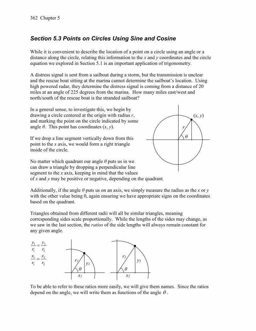
Section 5.3 Points on Circles Using Sine and Cosine While it is convenient to describe the location of a point on a circle using an angle or a distance along the circle, relating this information to the x and y coordinates and the circle equation we explored in Section 5.1 is an important application of trigonometry. A distress signal is sent from a sailboat during a storm, but the transmission is unclear and the rescue boat sitting at the marina cannot determine the sailboat’s location. Using high powered radar, they determine the distress signal is coming from a distance of 20 miles at an angle of 225 degrees from the marina. How many miles east/west and north/south of the rescue boat is the stranded sailboat? In a general sense, to investigate this, we begin by drawing a circle centered at the origin with radius r, and marking the point on the circle indicated by some angle θ. This point has coordinates (x, y). If we drop a line segment vertically down from this point to the x axis, we would form a right triangle inside of the circle. No matter which quadrant our angle θ puts us in we can draw a triangle by dropping a perpendicular line segment to the x axis, keeping in mind that the values of x and y may be positive or negative, depending on the quadrant. Additionally, if the angle θ puts us on an axis, we simply measure the radius as the x or y with the other value being 0, again ensuring we have appropriate signs on the coordinates based on the quadrant. Triangles obtained from different radii will all be similar triangles, meaning corresponding sides scale proportionally. While the lengths of the sides may change, as we saw in the last section, the ratios of the side lengths will always remain constant for any given angle.
1 2
1 2
y yr r=
1 2
1 2
x xr r=
To be able to refer to these ratios more easily, we will give them names. Since the ratios depend on the angle, we will write them as functions of the angle θ .
(x, y)
r
θ
r1
θ y1
x1
r2
θ
y2
x2

Section 5.3 Points on Circles Using Sine and Cosine 363
Sine and Cosine For the point (x, y) on a circle of radius r at an angle of θ , we can define two important functions as the ratios of the sides of the corresponding triangle:
The sine function: ry
=)sin(θ
The cosine function: rx
=)cos(θ
In this chapter, we will explore these functions using both circles and right triangles. In the next chapter, we will take a closer look at the behavior and characteristics of the sine and cosine functions. Example 1
The point (3, 4) is on the circle of radius 5 at some angle θ. Find )cos(θ and )sin(θ . Knowing the radius of the circle and coordinates of the point, we can evaluate the cosine and sine functions as the ratio of the sides.
53)cos( ==
rxθ
54)sin( ==
ryθ
There are a few cosine and sine values which we can determine fairly easily because the corresponding point on the circle falls on the x or y axis. Example 2
Find )90cos( ° and )90sin( ° On any circle, the terminal side of a 90 degree angle points straight up, so the coordinates of the corresponding point on the circle would be (0, r). Using our definitions of cosine and sine,
00)90cos( ===°rr
x
1)90sin( ===°rr
ry
(x, y)
r
θ y
x
r 90°
(0, r)

364 Chapter 5
Try it Now 1. Find cosine and sine of the angle π . Notice that the definitions above can also be stated as:
Coordinates of the Point on a Circle at a Given Angle On a circle of radius r at an angle of θ , we can find the coordinates of the point (x, y) at that angle using
)cos(θrx = )sin(θry =
On a unit circle, a circle with radius 1, )cos(θ=x and )sin(θ=y .
Utilizing the basic equation for a circle centered at the origin, 222 ryx =+ , combined with the relationships above, we can establish a new identity.
222 ryx =+ substituting the relations above, 222 ))sin(())cos(( rrr =+ θθ simplifying,
22222 ))(sin())(cos( rrr =+ θθ dividing by 2r 1))(sin())(cos( 22 =+ θθ or using shorthand notation
1)(sin)(cos 22 =+ θθ Here )(cos2 θ is a commonly used shorthand notation for 2))(cos(θ . Be aware that many calculators and computers do not understand the shorthand notation. In Section 5.1 we related the Pythagorean Theorem 222 cba =+ to the basic equation of a circle 222 ryx =+ , which we have now used to arrive at the Pythagorean Identity.
Pythagorean Identity The Pythagorean Identity. For any angle θ, 1)(sin)(cos 22 =+ θθ .
One use of this identity is that it helps us to find a cosine value of an angle if we know the sine value of that angle or vice versa. However, since the equation will yield two possible values, we will need to utilize additional knowledge of the angle to help us find the desired value.
Section 5.3 Points on Circles Using Sine and Cosine 365
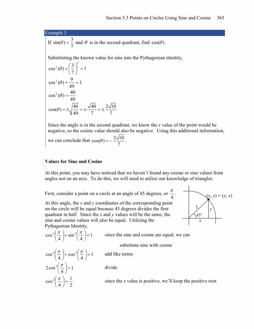
Example 3
If 73)sin( =θ and θ is in the second quadrant, find )cos(θ .
Substituting the known value for sine into the Pythagorean identity,
173)(cos
22 =
+θ
1499)(cos2 =+θ
4940)(cos2 =θ
40 40 2 10cos( )49 7 7
θ = ± = ± = ±
Since the angle is in the second quadrant, we know the x value of the point would be negative, so the cosine value should also be negative. Using this additional information,
we can conclude that 2 10cos( )7
θ = − .
Values for Sine and Cosine At this point, you may have noticed that we haven’t found any cosine or sine values from angles not on an axis. To do this, we will need to utilize our knowledge of triangles.
First, consider a point on a circle at an angle of 45 degrees, or 4π .
At this angle, the x and y coordinates of the corresponding point on the circle will be equal because 45 degrees divides the first quadrant in half. Since the x and y values will be the same, the sine and cosine values will also be equal. Utilizing the Pythagorean Identity,
14
sin4
cos 22 =
+
ππ since the sine and cosine are equal, we can
substitute sine with cosine
14
cos4
cos 22 =
+
ππ add like terms
14
cos2 2 =
π divide
21
4cos2 =
π since the x value is positive, we’ll keep the positive root
1 45°
y
x
(x, y) = (x, x)

366 Chapter 5
21
4cos =
π often this value is written with a rationalized denominator
Remember, to rationalize the denominator we multiply by a term equivalent to 1 to get rid of the radical in the denominator.
22
42
22
21
4cos ===
π
Since the sine and cosine are equal, 22
4sin =
π as well. The (x, y) coordinates for a
point on a circle of radius 1 at an angle of 45 degrees are
22,
22
.
Example 4
Find the coordinates of the point on a circle of radius 6 at an angle of 4π .
Using our new knowledge that 22
4sin =
π and
22
4cos =
π , along with our
relationships that stated )cos(θrx = and )sin(θry = , we can find the coordinates of the point desired:
23226
4cos6 =
=
=πx
23226
4sin6 =
=
=πy
Try it Now 2. Find the coordinates of the point on a circle of radius 3 at an angle of °90 . Next, we will find the cosine and sine at an angle of
30 degrees, or 6π . To do this, we will first draw a
triangle inside a circle with one side at an angle of 30 degrees, and another at an angle of -30 degrees. If the resulting two right triangles are combined into one
r
30°
(x, y)

Section 5.3 Points on Circles Using Sine and Cosine 367
large triangle, notice that all three angles of this larger triangle will be 60 degrees. Since all the angles are equal, the sides will all be equal as well. The vertical line has length 2y, and since the sides are all
equal we can conclude that 2y = r, or 2ry = . Using this, we
can find the sine value:
211
22
6sin =⋅===
rr
r
r
ryπ
Using the Pythagorean Identity, we can find the cosine value:
16
sin6
cos 22 =
+
ππ
121
6cos
22 =
+
π
43
6cos2 =
π since the x value is positive, we’ll keep the positive root
23
43
6cos ==
π
The (x, y) coordinates for the point on a circle of radius 1 at an angle of 30 degrees are
21,
23
.
By drawing a the triangle inside the unit circle with a 30 degree angle and reflecting it
over the line y = x, we can find the cosine and sine for 60 degrees, or 3π , without any
additional work.
By this symmetry, we can see the coordinates of the point on the unit circle at an angle of
60 degrees will be
23,
21
, giving
30°
21
23
1
y = x
30°
21
1
60°
y = x
23
60°
60°
60°
r
r
y
y

368 Chapter 5
21
3cos =
π and
23
3sin =
π
We have now found the cosine and sine values for all the commonly encountered angles in the first quadrant of the unit circle.
Angle 0 6π , or 30°
4π , or 45°
3π , or 60°
2π , or 90°
Cosine 1 32
22
12
0
Sine 0 12
22
32
1
For any given angle in the first quadrant, there will be an angle in another quadrant with the same sine value, and yet another angle in yet another quadrant with the same cosine value. Since the sine value is the y coordinate on the unit circle, the other angle with the same sine will share the same y value, but have the opposite x value. Likewise, the angle with the same cosine will share the same x value, but have the opposite y value. As shown here, angle α has the same sine value as angle θ; the cosine values would be opposites. The angle β has the same cosine value as the angle θ; the sine values would be opposites.
)sin()sin( αθ = and )cos()cos( αθ −= )sin()sin( βθ −= and )cos()cos( βθ =
It is important to notice the relationship between the angles. If, from the angle, you measured the smallest angle to the horizontal axis, all would have the same measure in absolute value. We say that all these angles have a reference angle of θ.
(x, y)
r θ α
(x, y)
r θ
β

Section 5.3 Points on Circles Using Sine and Cosine 369
Reference Angle An angle’s reference angle is the size of the smallest angle to the horizontal axis. A reference angle is always an angle between 0
and 90 degrees, or 0 and 2π radians.
Angles share the same cosine and sine values as their reference angles, except for signs (positive or negative) which can be determined from the quadrant of the angle.
Example 5
Find the reference angle of 150 degrees. Use it to find )150cos( ° and )150sin( ° . 150 degrees is located in the second quadrant. It is 30 degrees short of the horizontal axis at 180 degrees, so the reference angle is 30 degrees. This tells us that 150 degrees has the same sine and cosine values as 30 degrees, except
for sign. We know that 21)30sin( =° and
23)30cos( =° . Since 150 degrees is in the
second quadrant, the x coordinate of the point on the circle would be negative, so the cosine value will be negative. The y coordinate is positive, so the sine value will be positive.
21)150sin( =° and
23)150cos( −=°
The (x, y) coordinates for the point on a unit circle at an angle of °150 are
−21,
23
.
Using symmetry and reference angles, we can fill in cosine and sine values at the rest of the special angles on the unit circle. Take time to learn the (x, y) coordinates of all the major angles in the first quadrant!
(x, y)
θ
θ
θ
θ

370 Chapter 5
Example 6
Find the coordinates of the point on a circle of radius 12 at an angle of 6
7π .
Note that this angle is in the third quadrant, where both x and y are negative. Keeping this in mind can help you check your signs of the sine and cosine function.
362
3126
7cos12 −=
−=
=πx
62112
67sin12 −=
−=
=πy
The coordinates of the point are )6,36( −− .
Try it Now
3. Find the coordinates of the point on a circle of radius 5 at an angle of 53π .
3 130 , , ,
6 2 2
π°
2 245 , , ,
4 2 2
π°
1 360 , ,
3 2 2,π
°
( )90 , , 0 1
2,π
° 2 1 3120 , ,
3 2 2,π
° −
3 2 2135 , ,
4 2 2,π
° −
5 3 1150 , ,
6 2 2,π
° −
( )180 , , 1 0,π° −
5 2 2225 , ,
4 2 2,π
° − −
4 1 3240 , ,
3 2 2,π
° − −
( )3270 , , 0 1
2,π
° − 5 1 3
300 , ,3 2 2
,π°
−
7 2 2315 , ,
4 2 2,π
°
−
11 3 1330 , ,
6 2 2,π
°
−
( )( )
0 , 0, 1, 0
360 , 2 , 1, 0π
°
°
7 3 1210 , ,
6 2 2,π
° − −

Section 5.3 Points on Circles Using Sine and Cosine 371
Example 7 We now have the tools to return to the sailboat question posed at the beginning of this section. A distress signal is sent from a sailboat during a storm, but the transmission is unclear and the rescue boat sitting at the marina cannot determine the sailboat’s location. Using high powered radar, they determine the distress signal is coming from a point 20 miles away at an angle of 225 degrees from the marina. How many miles east/west and north/south of the rescue boat is the stranded sailboat? We can now answer the question by finding the coordinates of the point on a circle with a radius of 20 miles at an angle of 225 degrees.
( ) 142.142
220225cos20 −≈
−=°=x miles
( ) 142.142
220225sin20 −≈
−=°=y miles
The sailboat is located 14.142 miles west and 14.142 miles south of the marina.
The special values of sine and cosine in the first quadrant are very useful to know, since knowing them allows you to quickly evaluate the sine and cosine of very common angles without needing to look at a reference or use your calculator. However, scenarios do come up where we need to know the sine and cosine of other angles. To find the cosine and sine of any other angle, we turn to a computer or calculator. Be aware: most calculators can be set into “degree” or “radian” mode, which tells the calculator the units for the input value. When you evaluate “cos(30)” on your calculator, it will evaluate it as the cosine of 30 degrees if the calculator is in degree mode, or the cosine of 30 radians if the calculator is in radian mode. Most computer software with cosine and sine functions only operates in radian mode.
20 mi
225° E
W
N
S

372 Chapter 5
Example 8
Evaluate the cosine of 20 degrees using a calculator or computer. On a calculator that can be put in degree mode, you can evaluate this directly to be approximately 0.939693. On a computer or calculator without degree mode, you would first need to convert the
angle to radians, or equivalently evaluate the expression
⋅
18020cos π .
Important Topics of This Section The sine function The cosine function Pythagorean Identity Unit Circle values Reference angles Using technology to find points on a circle
Try it Now Answers 1. 1)cos( −=π 0)sin( =π
2. 313
2sin3
0032
cos3
=⋅=
=
=⋅=
=
π
π
y
x
3.
−=
235,
25
35sin5,
35cos5 ππ

Section 5.3 Points on Circles Using Sine and Cosine 373
Section 5.3 Exercises 1. Find the quadrant in which the terminal point determined by t lies if
a. sin( ) 0t < and cos( ) 0t < b. sin( ) 0t > and cos( ) 0t <
2. Find the quadrant in which the terminal point determined by t lies if a. sin( ) 0t < and cos( ) 0t > b. sin( ) 0t > and cos( ) 0t >
3. The point P is on the unit circle. If the y-coordinate of P is 35
, and P is in quadrant II,
find the x coordinate.
4. The point P is on the unit circle. If the x-coordinate of P is 15
, and P is in quadrant
IV, find the y coordinate.
5. If ( ) 1cos7
θ = and θ is in the 4th quadrant, find ( )sin θ .
6. If ( ) 2cos9
θ = and θ is in the 1st quadrant, find ( )sin θ .
7. If ( ) 3sin8
θ = and θ is in the 2nd quadrant, find ( )cos θ .
8. If ( ) 1sin4
θ = − and θ is in the 3rd quadrant, find ( )cos θ .
9. For each of the following angles, find the reference angle and which quadrant the
angle lies in. Then compute sine and cosine of the angle. a. 225° b. 300° c. 135° d. 210°
10. For each of the following angles, find the reference angle and which quadrant the angle lies in. Then compute sine and cosine of the angle. a. 120° b. 315° c. 250° d. 150°
11. For each of the following angles, find the reference angle and which quadrant the angle lies in. Then compute sine and cosine of the angle.
a. 54π b. 7
6π c. 5
3π d. 3
4π
12. For each of the following angles, find the reference angle and which quadrant the
angle lies in. Then compute sine and cosine of the angle.
a. 43π b. 2
3π c. 5
6π d. 7
4π

374 Chapter 5
13. Give exact values for ( )sin θ and ( )cos θ for each of these angles.
a. 34π
− b. 236π c.
2π
− d. 5π
14. Give exact values for ( )sin θ and ( )cos θ for each of these angles.
a. 23π
− b. 174π c.
6π
− d. 10π
15. Find an angle θ with 0 360θ< < ° or 0 2θ π< < that has the same sine value as:
a. 3π b. 80° c. 140° d. 4
3π e. 305°
16. Find an angle θ with 0 360θ< < ° or 0 2θ π< < that has the same sine value as:
a. 4π b. 15° c. 160° d. 7
6π e. 340°
17. Find an angle θ with 0 360θ< < ° or 0 2θ π< < that has the same cosine value as:
a. 3π b. 80° c. 140° d. 4
3π e. 305°
18. Find an angle θ with 0 360θ< < ° or 0 2θ π< < that has the same cosine value as:
a. 4π b. 15° c. 160° d. 7
6π e. 340°
19. Find the coordinates of the point on a circle with radius 15 corresponding to an angle
of 220°.
20. Find the coordinates of the point on a circle with radius 20 corresponding to an angle of 280°.
21. Marla is running clockwise around a circular track. She runs at a constant speed of 3 meters per second. She takes 46 seconds to complete one lap of the track. From her starting point, it takes her 12 seconds to reach the northernmost point of the track. Impose a coordinate system with the center of the track at the origin, and the northernmost point on the positive y-axis. [UW]
a) Give Marla’s coordinates at her starting point. b) Give Marla’s coordinates when she has been running for 10 seconds. c) Give Marla’s coordinates when she has been running for 901.3 seconds.

Section 5.4 The Other Trigonometric Functions 375
Section 5.4 The Other Trigonometric Functions In the previous section, we defined the sine and cosine functions as ratios of the sides of a right triangle in a circle. Since the triangle has 3 sides there are 6 possible combinations of ratios. While the sine and cosine are the two prominent ratios that can be formed, there are four others, and together they define the 6 trigonometric functions.
Tangent, Secant, Cosecant, and Cotangent Functions For the point (x, y) on a circle of radius r at an angle of θ , we can define four additional important functions as the ratios of the sides of the corresponding triangle:
The tangent function: xy
=)tan(θ
The secant function: xr
=)sec(θ
The cosecant function: yr
=)csc(θ
The cotangent function: yx
=)cot(θ
Geometrically, notice that the definition of tangent corresponds with the slope of the line segment between the origin (0, 0) and the point (x, y). This relationship can be very helpful in thinking about tangent values. You may also notice that the ratios defining the secant, cosecant, and cotangent are the reciprocals of the ratios defining the cosine, sine, and tangent functions, respectively. Additionally, notice that using our results from the last section,
)cos()sin(
)cos()sin()tan(
θθ
θθθ ===
rr
xy
Applying this concept to the other trig functions we can state the reciprocal identities.
Identities The other four trigonometric functions can be related back to the sine and cosine functions using these basic relationships:
)cos()sin()tan(
θθθ =
)cos(1)sec(θ
θ = )sin(
1)csc(θ
θ = 1 cos( )cot( )tan( ) sin( )
θθθ θ
= =
(x, y)
r
θ y
x
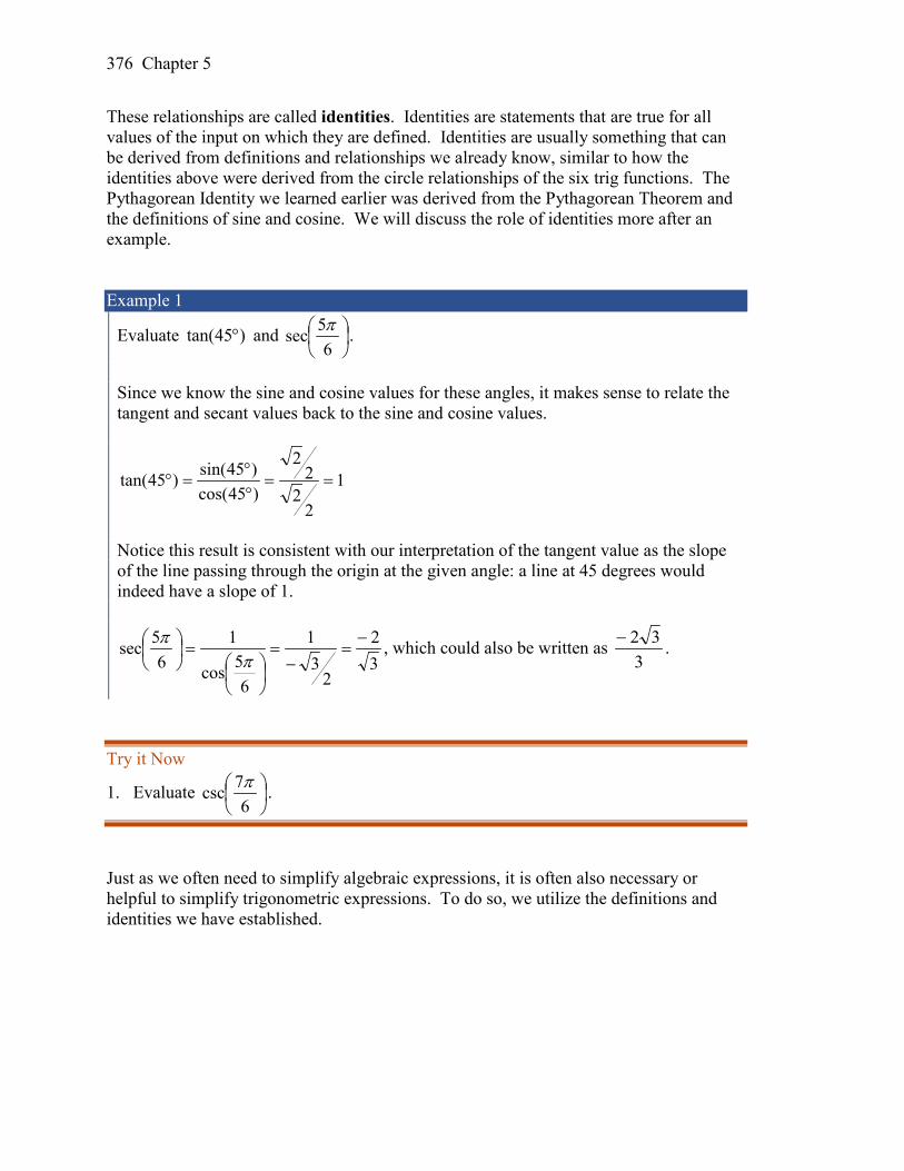
376 Chapter 5
These relationships are called identities. Identities are statements that are true for all values of the input on which they are defined. Identities are usually something that can be derived from definitions and relationships we already know, similar to how the identities above were derived from the circle relationships of the six trig functions. The Pythagorean Identity we learned earlier was derived from the Pythagorean Theorem and the definitions of sine and cosine. We will discuss the role of identities more after an example. Example 1
Evaluate )45tan( ° and
65sec π .
Since we know the sine and cosine values for these angles, it makes sense to relate the tangent and secant values back to the sine and cosine values.
1
22
22
)45cos()45sin()45tan( ==°°
=°
Notice this result is consistent with our interpretation of the tangent value as the slope of the line passing through the origin at the given angle: a line at 45 degrees would indeed have a slope of 1.
32
23
1
65cos
16
5sec −=
−=
=
ππ , which could also be written as
332− .
Try it Now
1. Evaluate
67csc π .
Just as we often need to simplify algebraic expressions, it is often also necessary or helpful to simplify trigonometric expressions. To do so, we utilize the definitions and identities we have established.

Section 5.4 The Other Trigonometric Functions 377
Example 2
Simplify ( )( )θθ
tansec .
We can simplify this by rewriting both functions in terms of sine and cosine
( )( )
( )( )
( )θθ
θθθ
cossin
cos1
tansec
= To divide the fractions we could invert and multiply
( )( )( )θθ
θ sincos
cos1
= cancelling the cosines,
( ) ( )θθ
cscsin
1== simplifying and using the identity
By showing that ( )( )θθ
tansec can be simplified to ( )θcsc , we have, in fact, established a new
identity: that ( )( ) ( )θθθ csc
tansec
= .
Occasionally a question may ask you to “prove the identity” or “establish the identity.” This is the same idea as when an algebra book asks a question like “show that
12)1( 22 +−=− xxx .” In this type of question, we must show the algebraic manipulations that demonstrate that the left and right side of the equation are in fact equal. You can think of a “prove the identity” problem as a simplification problem where you know the answer: you know what the end goal of the simplification should be, and just need to show the steps to get there. To prove an identity, in most cases you will start with the expression on one side of the identity and manipulate it using algebra and trigonometric identities until you have simplified it to the expression on the other side of the equation. Do not treat the identity like an equation to solve – it isn’t! The proof is establishing if the two expressions are equal, so we must take care to work with one side at a time rather than applying an operation simultaneously to both sides of the equation. Example 3
Prove the identity 1 cot( ) sin( ) cos( )csc( )
α α αα
+= + .
Since the left side seems a bit more complicated, we will start there and simplify the expression until we obtain the right side. We can use the right side as a guide for what might be good steps to make. In this case, the left side involves a fraction while the right side doesn’t, which suggests we should look to see if the fraction can be reduced.

378 Chapter 5
Additionally, since the right side involves sine and cosine and the left does not, it suggests that rewriting the cotangent and cosecant using sine and cosine might be a good idea. 1 cot( )
csc( )α
α+ Rewriting the cotangent and cosecant
cos( )1sin( )1
sin( )
αα
α
+= To divide the fractions, we invert and multiply
cos( ) sin( )1sin( ) 1
α αα
= +
Distributing,
sin( ) cos( ) sin( )11 sin( ) 1α α α
α= ⋅ + ⋅ Simplifying the fractions,
sin( ) cos( )α α= + Establishing the identity.
Notice that in the second step, we could have combined the 1 and cos( )sin( )
αα
before
inverting and multiplying. It is very common when proving or simplifying identities for there to be more than one way to obtain the same result.
We can also utilize identities we have previously learned, like the Pythagorean Identity, while simplifying or proving identities. Example 4
Establish the identity ( )( ) ( )θθθ sin1
sin1cos2
−=+
.
Since the left side of the identity is more complicated, it makes sense to start there. To simplify this, we will have to reduce the fraction, which would require the numerator to have a factor in common with the denominator. Additionally, we notice that the right side only involves sine. Both of these suggest that we need to convert the cosine into something involving sine. Recall the Pythagorean Identity told us 1)(sin)(cos 22 =+ θθ . By moving one of the trig functions to the other side, we can establish:
)(cos1)(sin 22 θθ −= and )(sin1)(cos 22 θθ −= Utilizing this, we now can establish the identity. We start on one side and manipulate:

Section 5.4 The Other Trigonometric Functions 379
( )( )θθ
sin1cos2
+ Utilizing the Pythagorean Identity
=( )( )θθ
sin1sin1 2
+−
Factoring the numerator
( )( ) ( )( )( )θ
θθsin1
sin1sin1+
+−= Cancelling the like factors
( )θsin1−= Establishing the identity We can also build new identities from previously established identities. For example, if we divide both sides of the Pythagorean Identity by cosine squared (which is allowed since we’ve already shown the identity is true),
)(cos1
)(cos)(sin)(cos
22
22
θθθθ
=+ Splitting the fraction on the left,
)(cos1
)(cos)(sin
)(cos)(cos
22
2
2
2
θθθ
θθ
=+ Simplifying and using the definitions of tan and sec
)(sec)(tan1 22 θθ =+ . Try it Now 2. Use a similar approach to establish that )(csc1)(cot 22 θθ =+ .
Identities Alternate forms of the Pythagorean Identity
)(sec)(tan1 22 θθ =+
)(csc1)(cot 22 θθ =+ Example 5
If 72)tan( =θ and θ is in the 3rd quadrant, find )cos(θ .
There are two approaches to this problem, both of which work equally well.

380 Chapter 5
Approach 1
Since xy
=)tan(θ and the angle is in the third quadrant, we can imagine a triangle in a
circle of some radius so that the point on the circle is (-7, -2), so 72
72=
−−
=xy .
Using the Pythagorean Theorem, we can find the radius of the circle:
222 )2()7( r=−+− , so 53=r . Now we can find the cosine value:
537)cos( −
==rxθ
Approach 2 Using the )(sec)(tan1 22 θθ =+ form of the Pythagorean Identity with the known tangent value,
)(sec)(tan1 22 θθ =+
)(sec721 2
2
θ=
+
)(sec4953 2 θ=
753
4953)sec( ±=±=θ
Since the angle is in the third quadrant, the cosine value will be negative so the secant value will also be negative. Keeping the negative result, and using definition of secant,
753)sec( −=θ
753
)cos(1
−=θ
Inverting both sides
53537
537)cos( −=−=θ
Try it Now
3. If 37)sec( −=φ and
2π φ π< < , find tan( )φ and sin( )φ .

Section 5.4 The Other Trigonometric Functions 381
Important Topics of This Section 6 Trigonometric Functions:
Sine Cosine Tangent Cosecant Secant Cotangent
Trig identities Try it Now Answers
1. 22
11
67sin
16
7csc −=−
=
=
ππ
2.
)(csc1)(cot
)(sin1
)(sin)(sin
)(sin)(cos
1sin
)(sin)(cos
22
22
2
2
2
2
22
θθ
θθθ
θθ
θθθ
=+
=+
=+
3. 37)sec( −=φ . By definition,
37
)cos(1
−=φ
, so 73)cos( −=φ .
Using Pythagorean Identity with the sec, 2
2
37)(tan1
−=+ φ . Solving gives
340)tan(−
=φ . We use the negative square root since an angle in the second quadrant
would have a negative tangent.
Using Pythagorean Identity with the cos, 173)(sin
22 =
−+φ . Solving,
740)sin( =φ .

382 Chapter 5
Section 5.4 Exercises
1. If 4πθ = , find exact values for ( ) ( ) ( ) ( )sec ,csc , tan , cot θ θ θ θ .
2. If 7 4πθ = , find exact values for ( ) ( ) ( ) ( )sec ,csc , tan , cot θ θ θ θ .
3. If 5 6πθ = , find exact values for ( ) ( ) ( ) ( )sec ,csc , tan , cot θ θ θ θ .
4. If 6πθ = , find exact values for ( ) ( ) ( ) ( )sec ,csc , tan , cotθ θ θ θ .
5. If 2 3πθ = , find exact values for ( ) ( ) ( ) ( )sec ,csc , tan , cot θ θ θ θ .
6. If 4 3πθ = , find exact values for ( ) ( ) ( ) ( )sec ,csc , tan , cotθ θ θ θ .
7. Evaluate: a. ( )sec 135° b. ( )csc 210° c. ( )tan 60° d. ( )cot 225°
8. Evaluate: a. ( )sec 30° b. ( )csc 315° c. ( )tan 135° d. ( )cot 150°
9. If ( ) 3sin4
θ = , and θ is in quadrant II, find ( ) ( ) ( ) ( ) ( )cos , sec ,csc , tan , cotθ θ θ θ θ .
10. If ( ) 2sin7
θ = , and θ is in quadrant II, find ( ) ( ) ( ) ( ) ( )cos , sec ,csc , tan , cotθ θ θ θ θ .
11. If ( ) 1cos3
θ = − , and θ is in quadrant III, find
( ) ( ) ( ) ( ) ( )sin , sec ,csc , tan , cotθ θ θ θ θ .
12. If ( ) 1cos5
θ = , and θ is in quadrant I, find ( ) ( ) ( ) ( ) ( )sin , sec ,csc , tan , cotθ θ θ θ θ .
13. If ( ) 12tan5
θ = , and 02πθ≤ < , find ( ) ( ) ( ) ( ) ( )sin , cos ,sec , csc , cotθ θ θ θ θ .
14. If ( )tan 4θ = , and 02πθ≤ < , find ( ) ( ) ( ) ( ) ( )sin , cos ,sec , csc , cotθ θ θ θ θ .

Section 5.4 The Other Trigonometric Functions 383
15. Use a calculator to find sine, cosine, and tangent of the following values:
a. 0.15 b. 4 c. 70° d. 283°
16. Use a calculator to find sine, cosine, and tangent of the following values:
a. 0.5 b. 5.2 c. 10° d. 195°
Simplify each of the following to an expression involving a single trig function with no fractions. 17. ( )csc( ) tant t
18. ( )cos( )csct t
19. ( )( )
seccsc
tt
20. ( )( )
cotcsc
tt
21. ( ) ( )( )
sec cossint t
t−
22. ( )( ) ( )tan
sec cost
t t−
23. ( )( )
1 cot1 tan
tt
++
24. ( )( )
1 sin1 csc
tt
++
25. ( ) ( )
( )
2 2
2
sin coscost t
t+
26. ( )
( )
2
2
1 sinsin
tt
−

384 Chapter 5
Prove the identities.
27. ( )( ) ( )
2sin1 cos
1 cosθ
θθ
= −+
28. ( )
22
1tan ( ) 1cos
tt
= −
29. ( ) ( ) ( ) ( )sec cos sin tana a a a− =
30. ( )
( )
22
2
1 tancsc ( )
tanb
bb
+=
31. ( ) ( )( ) ( ) ( ) ( )
2 2csc sincos cot
csc sinx x
x xx x−
=+
32. ( ) ( )( ) ( ) ( ) ( )sin cos
sin cossec csc
θ θθ θ
θ θ−
=−
33. ( )
( ) ( ) ( )2
2
csc 11 sin
csc cscα
αα α
−= +
−
34. ( ) ( ) ( ) ( )( )1 cot cos sec cscx x x x+ = +
35. ( )( )
( )( )
1 cos sinsin 1 cos
u uu u
+=
−
36. ( ) ( )( ) ( )
22
1 sin 12seccos 1 sin
tt
t t−
= +−
37. ( ) ( )( ) ( ) ( ) ( )
4 4sin cossin cos
sin cosγ γ
γ γγ γ
−= +
−
38. ( )( ) ( )( )
( ) ( )1 cos 1 cos
sinsinA A
AA
+ −=

Section 5.5 Right Triangle Trigonometry 385
Section 5.5 Right Triangle Trigonometry In section 5.3 we were introduced to the sine and cosine function as ratios of the sides of a triangle drawn inside a circle, and spent the rest of that section discussing the role of those functions in finding points on the circle. In this section, we return to the triangle, and explore the applications of the trigonometric functions to right triangles where circles may not be involved. Recall that we defined sine and cosine as
ry
=)sin(θ
rx
=)cos(θ
Separating the triangle from the circle, we can make equivalent but more general definitions of the sine, cosine, and tangent on a right triangle. On the right triangle, we will label the hypotenuse as well as the side opposite the angle and the side adjacent (next to) the angle.
Right Triangle Relationships Given a right triangle with an angle of θ
hypotenuseopposite)sin( =θ
hypotenuseadjacent)cos( =θ
adjacentopposite)tan( =θ
A common mnemonic for remembering these relationships is SohCahToa, formed from the first letters of “Sine is opposite over hypotenuse, Cosine is adjacent over hypotenuse, Tangent is opposite over adjacent.”
(x, y)
r
θ y
x
θ
adjacent
opposite hypotenuse

386 Chapter 5
Example 1 Given the triangle shown, find the value for )cos(α . The side adjacent to the angle is 15, and the hypotenuse of the triangle is 17, so
1715
hypotenuseadjacent)cos( ==α
When working with general right triangles, the same rules apply regardless of the orientation of the triangle. In fact, we can evaluate the sine and cosine of either of the two acute angles in the triangle.
Example 2
Using the triangle shown, evaluate )cos(α , )sin(α , )cos(β , and )sin(β .
53
hypotenuse oadjacent t)cos( ==αα
54
hypotenuse opposite)sin( ==αα
54
hypotenuse oadjacent t)cos( ==ββ
53
hypotenuse opposite)sin( ==ββ
Try it Now 1. A right triangle is drawn with angle α opposite a side with length 33, angle β
opposite a side with length 56, and hypotenuse 65. Find the sine and cosine of α andβ .
α β
Adjacent to α Opposite β
Hypotenuse
Adjacent to β Opposite α
α
15
8 17
α β
3
5
4

Section 5.5 Right Triangle Trigonometry 387
You may have noticed that in the above example that )sin()cos( βα = and )sin()cos( αβ = . This makes sense since the side opposite α is also adjacent to β. Since
the three angles in a triangle need to add to π, or 180 degrees, then the other two angles
must add to 2π , or 90 degrees, so απβ −=
2, and βπα −=
2. Since )sin()cos( βα = ,
then
−= απα
2sin)cos( .
Cofunction Identities The cofunction identities for sine and cosine are:
−= θπθ
2sin)cos(
−= θπθ
2cos)sin(
In the previous examples, we evaluated the sine and cosine on triangles where we knew all three sides of the triangle. Right triangle trigonometry becomes powerful when we start looking at triangles in which we know an angle but don’t know all the sides. Example 3
Find the unknown sides of the triangle pictured here.
Since hypotenuse
opposite)sin( =θ , b7)30sin( =° .
From this, we can solve for the side b.
7)30sin( =°b
)30sin(7
°=b
To obtain a value, we can evaluate the sine and simplify
142
17
==b
To find the value for side a, we could use the cosine, or simply apply the Pythagorean Theorem:
222 7 ba =+ 222 147 =+a
147=a
30°
a
7
b

388 Chapter 5
Notice that if we know at least one of the non-right angles of a right triangle and one side, we can find the rest of the sides and angles. Try it Now
2. A right triangle has one angle of 3π and a hypotenuse of 20. Find the unknown sides
and angles of the triangle. Example 4
To find the height of a tree, a person walks to a point 30 feet from the base of the tree, and measures the angle from the ground to the top of the tree to be 57 degrees. Find the height of the tree. We can introduce a variable, h, to represent the height of the tree. The two sides of the triangle that are most important to us are the side opposite the angle, the height of the tree we are looking for, and the adjacent side, the side we are told is 30 feet long. The trigonometric function which relates the side opposite of the angle and the side adjacent to the angle is the tangent.
30adjacentopposite)57tan( h
==° Solving for h,
)57tan(30 °=h Using technology, we can approximate a value 2.46)57tan(30 ≈°=h feet
The tree is approximately 46 feet tall.
Example 5
A person standing on the roof of a 100 foot tall building is looking towards a skyscraper a few blocks away, wondering how tall it is. She measures the angle of declination from the roof of the building to the base of the skyscraper to be 20 degrees and the angle of inclination to the top of the skyscraper to be 42 degrees.
57°
30 feet

Section 5.5 Right Triangle Trigonometry 389
To approach this problem, it would be good to start with a picture. Although we are interested in the height, h, of the skyscraper, it can be helpful to also label other unknown quantities in the picture – in this case the horizontal distance x between the buildings and a, the height of the skyscraper above the person. To start solving this problem, notice we have two right triangles. In the top triangle, we know one angle is 42 degrees, but we don’t know any of the sides of the triangle, so we don’t yet know enough to work with this triangle. In the lower right triangle, we know one angle is 20 degrees, and we know the vertical height measurement of 100 ft. Since we know these two pieces of information, we can solve for the unknown distance x.
x100
adjacentopposite)20tan( ==° Solving for x
100)20tan( =°x
)20tan(100
°=x
Now that we have found the distance x, we know enough information to solve the top right triangle.
)20tan(100adjacent
opposite)42tan(°
===°a
xa
100)20tan()42tan( °
=°a
)20tan()42tan(100 °=° a
a=°°
)20tan()42tan(100
Approximating a value,
4.247)20tan(
)42tan(100≈
°°
=a feet
Adding the height of the first building, we determine that the skyscraper is about 347 feet tall.
100 ft
h a
x 42°
20° 100 ft

390 Chapter 5
Important Topics of This Section SOH CAH TOA Cofunction identities Applications with right triangles
Try it Now Answers
1. 33sin( )65
α = 56cos( )65
α = 56sin( )65
β = 6533)cos( =β
2. 20Adj
hypoteuseadjacent
3cos ==
π so, 10
2120
3cos20adjacent =
=
=π
20
OpphypoteuseOpposite
3sin ==
π so, 310
2320
3sin20opposite =
=
=π
Missing angle = 180-90-60 = 30 degrees or 6π .

Section 5.5 Right Triangle Trigonometry 391
Section 5.5 Exercises Note: pictures may not be drawn to scale. In each of the triangles below, find ( ) ( ) ( ) ( ) ( ) ( )sin ,cos , tan ,sec ,csc ,cotA A A A A A . 1. 2. In each of the following triangles, solve for the unknown sides and angles. 3. 4.
5. 6.
7. 8. 9. A 33-ft ladder leans against a building so that the angle between the ground and the
ladder is 80°. How high does the ladder reach up the side of the building? 10. A 23-ft ladder leans against a building so that the angle between the ground and the
ladder is 80°. How high does the ladder reach up the side of the building?
60°
a 10
c A
10° b
a 12 B
65°
b a
10
B
A 8
10
A
10
4
30°
7 c B
b
35° 7
c B
b
62°
a 10
c A

392 Chapter 5
11. The angle of elevation to the top of a building in New York is found to be 9 degrees from the ground at a distance of 1 mile from the base of the building. Using this information, find the height of the building.
12. The angle of elevation to the top of a building in Seattle is found to be 2 degrees from the ground at a distance of 2 miles from the base of the building. Using this information, find the height of the building.
13. A radio tower is located 400 feet from a building. From a window in the building, a person determines that the angle of elevation to the top of the tower is 36° and that the angle of depression to the bottom of the tower is 23°. How tall is the tower?
14. A radio tower is located 325 feet from a building. From a window in the building, a person determines that the angle of elevation to the top of the tower is 43° and that the angle of depression to the bottom of the tower is 31°. How tall is the tower?
15. A 200 foot tall monument is located in the distance. From a window in a building, a person determines that the angle of elevation to the top of the monument is 15° and that the angle of depression to the bottom of the tower is 2°. How far is the person from the monument?
16. A 400 foot tall monument is located in the distance. From a window in a building, a person determines that the angle of elevation to the top of the monument is 18° and that the angle of depression to the bottom of the tower is 3°. How far is the person from the monument?
17. There is an antenna on the top of a building. From a location 300 feet from the base of the building, the angle of elevation to the top of the building is measured to be 40°. From the same location, the angle of elevation to the top of the antenna is measured to be 43°. Find the height of the antenna.
18. There is lightning rod on the top of a building. From a location 500 feet from the
base of the building, the angle of elevation to the top of the building is measured to be 36°. From the same location, the angle of elevation to the top of the lightning rod is measured to be 38°. Find the height of the lightning rod.
19. Find the length x. 20. Find the length x.
x
85
36° 50°
x
82
63° 39°

Section 5.5 Right Triangle Trigonometry 393
21. Find the length x. 22. Find the length x.
23. A plane is flying 2000 feet above sea level
toward a mountain. The pilot observes the top of the mountain to be 18o above the horizontal, then immediately flies the plane at an angle of 20o above horizontal. The airspeed of the plane is 100 mph. After 5 minutes, the plane is directly above the top of the mountain. How high is the plane above the top of the mountain (when it passes over)? What is the height of the mountain? [UW]
24. Three airplanes depart SeaTac Airport. A United flight is heading in a direction 50°
counterclockwise from east, an Alaska flight is heading 115° counterclockwise from east and a Delta flight is heading 20° clockwise from east. [UW]
a. Find the location of the United flight when it is 20 miles north of SeaTac. b. Find the location of the Alaska flight when it is 50 miles west of SeaTac. c. Find the location of the Delta flight when it is 30 miles east of SeaTac.
(a) The flight paths of three airplanes
(b) Modeling the paths of each flight
Alaska United
Delta
Alaska United
Delta
x
119
70° 26°
x
115
56° 35°
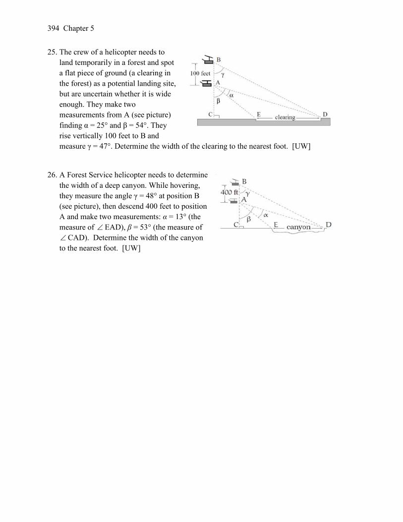
394 Chapter 5
25. The crew of a helicopter needs to land temporarily in a forest and spot a flat piece of ground (a clearing in the forest) as a potential landing site, but are uncertain whether it is wide enough. They make two measurements from A (see picture) finding α = 25° and β = 54°. They rise vertically 100 feet to B and measure γ = 47°. Determine the width of the clearing to the nearest foot. [UW]
26. A Forest Service helicopter needs to determine
the width of a deep canyon. While hovering, they measure the angle γ = 48° at position B (see picture), then descend 400 feet to position A and make two measurements: α = 13° (the measure of ∠EAD), β = 53° (the measure of ∠CAD). Determine the width of the canyon to the nearest foot. [UW]

This chapter is part of Precalculus: An Investigation of Functions © Lippman & Rasmussen 2017. This material is licensed under a Creative Commons CC-BY-SA license.
Chapter 6: Periodic Functions In the previous chapter, the trigonometric functions were introduced as ratios of sides of a right triangle, and related to points on a circle. We noticed how the x and y values of the points did not change with repeated revolutions around the circle by finding coterminal angles. In this chapter, we will take a closer look at the important characteristics and applications of these types of functions, and begin solving equations involving them.
Section 6.1 Sinusoidal Graphs .................................................................................... 395 Section 6.2 Graphs of the Other Trig Functions ......................................................... 412 Section 6.3 Inverse Trig Functions ............................................................................. 422 Section 6.4 Solving Trig Equations ............................................................................ 430 Section 6.5 Modeling with Trigonometric Equations ................................................. 441
Section 6.1 Sinusoidal Graphs The London Eye1 is a huge Ferris wheel 135 meters (394 feet) tall in London, England, which completes one rotation every 30 minutes. When we look at the behavior of this Ferris wheel it is clear that it completes 1 cycle, or 1 revolution, and then repeats this revolution over and over again. This is an example of a periodic function, because the Ferris wheel repeats its revolution or one cycle every 30 minutes, and so we say it has a period of 30 minutes. In this section, we will work to sketch a graph of a rider’s height above the ground over time and express this height as a function of time.
Periodic Functions A periodic function is a function for which a specific horizontal shift, P, results in the original function: )()( xfPxf =+ for all values of x. When this occurs we call the smallest such horizontal shift with P > 0 the period of the function.
1 London Eye photo by authors, 2010, CC-BY

396 Chapter 6
You might immediately guess that there is a connection here to finding points on a circle, since the height above ground would correspond to the y value of a point on the circle. We can determine the y value by using the sine function. To get a better sense of this function’s behavior, we can create a table of values we know, and use them to sketch a graph of the sine and cosine functions. Listing some of the values for sine and cosine on a unit circle, θ 0
6π
4π
3π
2π
3
2π
43π
6
5π
π
cos 1
23
22 2
1
0 21
− 22
− 23
− -1
sin 0 21
22
23
1
23
22 2
1
0
Here you can see how for each angle, we use the y value of the point on the circle to determine the output value of the sine function.
Plotting more points gives the full shape of the sine and cosine functions.
6π
4π
3π
2π
θ
f(θ) = sin(θ)

Section 6.1 Sinusoidal Graphs 397
Notice how the sine values are positive between 0 and π, which correspond to the values of sine in quadrants 1 and 2 on the unit circle, and the sine values are negative between π and 2π, corresponding to quadrants 3 and 4.
Like the sine function we can track the value of the cosine function through the 4 quadrants of the unit circle as we place it on a graph. Both of these functions are defined for all real numbers, since we can evaluate the sine and cosine of any angle. By thinking of sine and cosine as coordinates of points on a unit circle, it becomes clear that the range of both functions must be the interval ]1,1[− .
Domain and Range of Sine and Cosine The domain of sine and cosine is all real numbers, ( , )−∞ ∞ . The range of sine and cosine is the interval [-1, 1].
Both these graphs are called sinusoidal graphs. In both graphs, the shape of the graph begins repeating after 2π. Indeed, since any coterminal angles will have the same sine and cosine values, we could conclude that
)sin()2sin( θπθ =+ and )cos()2cos( θπθ =+ . In other words, if you were to shift either graph horizontally by 2π, the resulting shape would be identical to the original function. Sinusoidal functions are a specific type of periodic function.
Period of Sine and Cosine The periods of the sine and cosine functions are both 2π.

398 Chapter 6
Looking at these functions on a domain centered at the vertical axis helps reveal symmetries. sine cosine
The sine function is symmetric about the origin, the same symmetry the cubic function has, making it an odd function. The cosine function is clearly symmetric about the y axis, the same symmetry as the quadratic function, making it an even function.
Negative Angle Identities The sine is an odd function, symmetric about the origin, so )sin()sin( θθ −=− .
The cosine is an even function, symmetric about the y-axis, so )cos()cos( θθ =− . These identities can be used, among other purposes, for helping with simplification and proving identities.
You may recall the cofunction identity from last chapter,
−= θπθ
2cos)sin( .
Graphically, this tells us that the sine and cosine graphs are horizontal transformations of each other. We can prove this by using the cofunction identity and the negative angle identity for cosine.
−=
−−=
+−=
−=
2cos
2cos
2cos
2cos)sin( πθπθπθθπθ
Now we can clearly see that if we horizontally shift the cosine function to the right by π/2 we get the sine function. Remember this shift is not representing the period of the function. It only shows that the cosine and sine function are transformations of each other.

Section 6.1 Sinusoidal Graphs 399
Example 1
Simplify )tan()sin(
θθ− .
We start by using the negative angle identity for sine.
)tan()sin(
θθ− Rewriting the tangent
)cos()sin(
)sin(
θθ
θ− Inverting and multiplying
)sin()cos()sin(
θθθ ⋅− Simplifying we get
)cos(θ− Transforming Sine and Cosine Example 2
A point rotates around a circle of radius 3. Sketch a graph of the y coordinate of the point. Recall that for a point on a circle of radius r, the y coordinate of the point is
)sin(θry = , so in this case, we get the equation )sin(3)( θθ =y . The constant 3 causes a vertical stretch of the y values of the function by a factor of 3. Notice that the period of the function does not change.
Since the outputs of the graph will now oscillate between -3 and 3, we say that the amplitude of the sine wave is 3. Try it Now 1. What is the amplitude of the function )cos(7)( θθ =f ? Sketch a graph of this
function.

400 Chapter 6
Example 3 A circle with radius 3 feet is mounted with its center 4 feet off the ground. The point closest to the ground is labeled P. Sketch a graph of the height above ground of the point P as the circle is rotated, then find a function that gives the height in terms of the angle of rotation. Sketching the height, we note that it will start 1 foot above the ground, then increase up to 7 feet above the ground, and continue to oscillate 3 feet above and below the center value of 4 feet. Although we could use a transformation of either the sine or cosine function, we start by looking for characteristics that would make one function easier to use than the other. We decide to use a cosine function because it starts at the highest or lowest value, while a sine function starts at the middle value. A standard cosine starts at the highest value, and this graph starts at the lowest value, so we need to incorporate a vertical reflection. Second, we see that the graph oscillates 3 above and below the center, while a basic cosine has an amplitude of one, so this graph has been vertically stretched by 3, as in the last example. Finally, to move the center of the circle up to a height of 4, the graph has been vertically shifted up by 4. Putting these transformations together,
4)cos(3)( +−= θθh
Midline The center value of a sinusoidal function, the value that the function oscillates above and below, is called the midline of the function, corresponding to a vertical shift. The function kf += )cos()( θθ has midline at y = k.
Try it Now 2. What is the midline of the function 4)cos(3)( −= θθf ? Sketch a graph of the
function.
3 ft
4 ft
P

Section 6.1 Sinusoidal Graphs 401
To answer the Ferris wheel problem at the beginning of the section, we need to be able to express our sine and cosine functions at inputs of time. To do so, we will utilize composition. Since the sine function takes an input of an angle, we will look for a function that takes time as an input and outputs an angle. If we can find a suitable )(tθfunction, then we can compose this with our )cos()( θθ =f function to obtain a sinusoidal function of time: ))(cos()( ttf θ= . Example 4
A point completes 1 revolution every 2 minutes around a circle of radius 5. Find the x coordinate of the point as a function of time, if it starts at (5, 0). Normally, we would express the x coordinate of a point on a unit circle using
)cos(θrx = , here we write the function )cos(5)( θθ =x . The rotation rate of 1 revolution every 2 minutes is an angular velocity. We can use this rate to find a formula for the angle as a function of time. The point begins at an angle of 0. Since the point rotates 1 revolution = 2π radians every 2 minutes, it rotates π radians every minute. After t minutes, it will have rotated:
tt πθ =)( radians Composing this with the cosine function, we obtain a function of time.
)cos(5))(cos(5)( tttx πθ == Notice that this composition has the effect of a horizontal compression, changing the period of the function. To see how the period relates to the stretch or compression coefficient B in the equation
( )Bttf sin)( = , note that the period will be the time it takes to complete one full revolution of a circle. If a point takes P minutes to complete 1 revolution, then the
angular velocity is minutesradians2
Pπ . Then t
Pt πθ 2)( = . Composing with a sine function,
== t
Pttf πθ 2sin))(sin()(
From this, we can determine the relationship between the coefficient B and the period:
PB π2= .
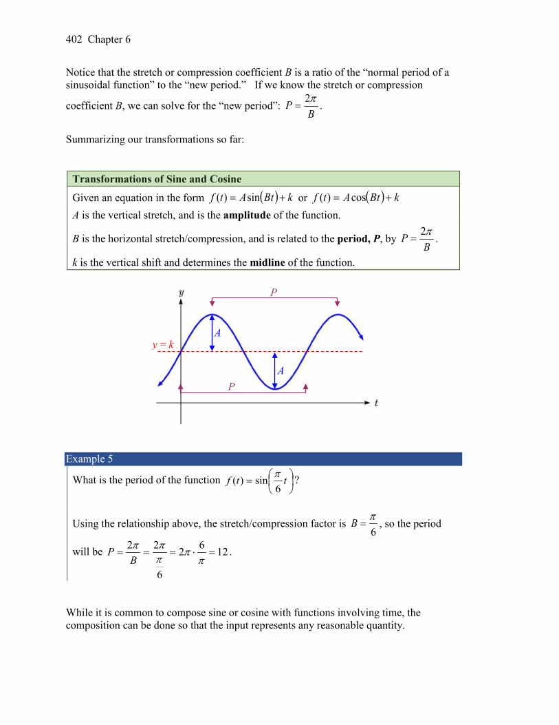
402 Chapter 6
Notice that the stretch or compression coefficient B is a ratio of the “normal period of a sinusoidal function” to the “new period.” If we know the stretch or compression
coefficient B, we can solve for the “new period”: B
P π2= .
Summarizing our transformations so far:
Transformations of Sine and Cosine
Given an equation in the form ( ) kBtAtf += sin)( or ( ) kBtAtf += cos)( A is the vertical stretch, and is the amplitude of the function.
B is the horizontal stretch/compression, and is related to the period, P, by B
P π2= .
k is the vertical shift and determines the midline of the function.
Example 5
What is the period of the function
= ttf
6sin)( π ?
Using the relationship above, the stretch/compression factor is 6π
=B , so the period
will be 1262
6
22=⋅===
ππ
πππ
BP .
While it is common to compose sine or cosine with functions involving time, the composition can be done so that the input represents any reasonable quantity.
y = k A
A
P
P

Section 6.1 Sinusoidal Graphs 403
Example 6 A bicycle wheel with radius 14 inches has the bottom-most point on the wheel marked in red. The wheel then begins rolling down the street. Write a formula for the height above ground of the red point after the bicycle has travelled x inches. The height of the point begins at the lowest value, 0, increases to the highest value of 28 inches, and continues to oscillate above and below a center height of 14 inches. In terms of the angle of rotation, θ:
14)cos(14)( +−= θθh In this case, x is representing a linear distance the wheel has travelled, corresponding to an arclength along the circle. Since arclength and angle can be related by θrs = , in this case we can write θ14=x , which allows us to express the angle in terms of x:
14)( xx =θ
Composing this with our cosine-based function from above,
14141cos1414
14cos14))(()( +
−=+
−== xxxhxh θ
The period of this function would be ππππ 28142
141
22=⋅===
BP , the circumference
of the circle. This makes sense – the wheel completes one full revolution after the bicycle has travelled a distance equivalent to the circumference of the wheel.
Example 7
Determine the midline, amplitude, and period of the function ( ) 12sin3)( += ttf . The amplitude is 3
The period is πππ===
222
BP
The midline is at 1y = Amplitude, midline, and period, when combined with vertical flips, allow us to write equations for a variety of sinusoidal situations.
θ
Starting
Rotated by θ
14in
x

404 Chapter 6
Try it Now 3. If a sinusoidal function starts on the midline at point (0,3), has an amplitude of 2, and
a period of 4, write a formula for the function Example 8
Find a formula for the sinusoidal function graphed here. The graph oscillates from a low of -1 to a high of 3, putting the midline at y = 1, halfway between. The amplitude will be 2, the distance from the midline to the highest value (or lowest value) of the graph. The period of the graph is 8. We can measure this from the first peak at x = -2 to the second at x = 6. Since the period is 8, the stretch/compression factor we will use will be
4822 πππ
===P
B
At x = 0, the graph is at the midline value, which tells us the graph can most easily be represented as a sine function. Since the graph then decreases, this must be a vertical reflection of the sine function. Putting this all together,
14
sin2)( +
−= ttf π
With these transformations, we are ready to answer the Ferris wheel problem from the beginning of the section. Example 9
The London Eye is a huge Ferris wheel in London, England, which completes one rotation every 30 minutes. The diameter of the wheel is 120 meters, but the passenger capsules sit outside the wheel. Suppose the diameter at the capsules is 130 meters, and riders board from a platform 5 meters above the ground. Express a rider’s height above ground as a function of time in minutes. It can often help to sketch a graph of the situation before trying to find the equation.

Section 6.1 Sinusoidal Graphs 405
With a diameter of 130 meters, the wheel has a radius of 65 meters. The height will oscillate with amplitude of 65 meters above and below the center. Passengers board 5 meters above ground level, so the center of the wheel must be located 65 + 5 = 70 meters above ground level. The midline of the oscillation will be at 70 meters. The wheel takes 30 minutes to complete 1 revolution, so the height will oscillate with period of 30 minutes. Lastly, since the rider boards at the lowest point, the height will start at the smallest value and increase, following the shape of a flipped cosine curve. Putting these together: Amplitude: 65 Midline: 70
Period: 30, so 1530
2 ππ==B
Shape: negative cosine An equation for the rider’s height would be
( ) 65cos 7015
h t tπ = − +
Try it Now 4. The Ferris wheel at the Puyallup Fair2 has a diameter of about 70
feet and takes 3 minutes to complete a full rotation. Passengers board from a platform 10 feet above the ground. Write an equation for a rider’s height above ground over time.
While these transformations are sufficient to represent many situations, occasionally we encounter a sinusoidal function that does not have a vertical intercept at the lowest point, highest point, or midline. In these cases, we need to use horizontal shifts. Since we are combining horizontal shifts with horizontal stretches, we need to be careful. Recall that when the inside of the function is factored, it reveals the horizontal shift.
2 Photo by photogirl7.1, http://www.flickr.com/photos/kitkaphotogirl/432886205/sizes/z/, CC-BY

406 Chapter 6
Horizontal Shifts of Sine and Cosine
Given an equation in the form ( ) khtBAtf +−= )(sin)( or ( ) khtBAtf +−= )(cos)( h is the horizontal shift of the function
Example 10
Sketch a graph of
−=
44sin3)( ππ ttf .
To reveal the horizontal shift, we first need to factor inside the function:
−= )1(
4sin3)( ttf π
This graph will have the shape of a sine function, starting at the midline and increasing,
with an amplitude of 3. The period of the graph will be 842
4
22=⋅===
ππ
πππ
BP .
Finally, the graph will be shifted to the right by 1.
In some physics and mathematics books, you will hear the horizontal shift referred to as phase shift. In other physics and mathematics books, they would say the phase shift of
the equation above is 4π , the value in the unfactored form. Because of this ambiguity, we
will not use the term phase shift any further, and will only talk about the horizontal shift.

Section 6.1 Sinusoidal Graphs 407
Example 11 Find a formula for the function graphed here. With highest value at 1 and lowest value at -5, the midline will be halfway between at -2. The distance from the midline to the highest or lowest value gives an amplitude of 3. The period of the graph is 6, which can be measured from the peak at x = 1 to the next peak at x = 7, or from the distance between the lowest
points. This gives 36
22 πππ===
PB .
For the shape and shift, we have more than one option. We could either write this as: A cosine shifted 1 to the right A negative cosine shifted 2 to the left A sine shifted ½ to the left A negative sine shifted 2.5 to the right While any of these would be fine, the cosine shifts are easier to work with than the sine shifts in this case, because they involve integer values. Writing these:
2)1(3
cos3)( −
−= xxy π or
2)2(3
cos3)( −
+−= xxy π
Again, these functions are equivalent, so both yield the same graph.
Try it Now 5. Write a formula for the function graphed here.
408 Chapter 6
Important Topics of This Section Periodic functions Sine and cosine function from the unit circle Domain and range of sine and cosine functions Sinusoidal functions Negative angle identity Simplifying expressions Transformations Amplitude Midline Period Horizontal shifts
Try it Now Answers 1. 7
2. -4
3. ( ) 2sin 32
f x xπ = +
4. 2( ) 35cos 453
h t tπ = − +
5. Two possibilities: ( ) 4cos ( 3.5) 45
f x xπ = − +
or ( ) 4sin ( 1) 45
f x xπ = − +

Section 6.1 Sinusoidal Graphs 409
Section 6.1 Exercises 1. Sketch a graph of ( ) ( )3sinf x x= − .
2. Sketch a graph of ( ) ( )4sinf x x= .
3. Sketch a graph of ( ) ( )2cosf x x= .
4. Sketch a graph of ( ) ( )4cosf x x= − . For the graphs below, determine the amplitude, midline, and period, then find a formula for the function.
5. 6.
7. 8.
9. 10.

410 Chapter 6
For each of the following equations, find the amplitude, period, horizontal shift, and midline. 11. 3sin(8( 4)) 5y x= + +
12. 4sin ( 3) 72
y xπ = − +
13. 2sin(3 21) 4y x= − + 14. 5sin(5 20) 2y x= + −
15. sin 36
y xπ π = + −
16. 7 78sin 66 2
y xπ π = + +
Find a formula for each of the functions graphed below.
17.
18.

Section 6.1 Sinusoidal Graphs 411
19.
20. 21. Outside temperature over the course of a day can be modeled as a sinusoidal function.
Suppose you know the temperature is 50 degrees at midnight and the high and low temperature during the day are 57 and 43 degrees, respectively. Assuming t is the number of hours since midnight, find a function for the temperature, D, in terms of t.
22. Outside temperature over the course of a day can be modeled as a sinusoidal function. Suppose you know the temperature is 68 degrees at midnight and the high and low temperature during the day are 80 and 56 degrees, respectively. Assuming t is the number of hours since midnight, find a function for the temperature, D, in terms of t.
23. A Ferris wheel is 25 meters in diameter and boarded from a platform that is 1 meters
above the ground. The six o'clock position on the Ferris wheel is level with the loading platform. The wheel completes 1 full revolution in 10 minutes. The function
( )h t gives your height in meters above the ground t minutes after the wheel begins to turn.
a. Find the amplitude, midline, and period of ( )h t .
b. Find a formula for the height function ( )h t . c. How high are you off the ground after 5 minutes?
24. A Ferris wheel is 35 meters in diameter and boarded from a platform that is 3 meters
above the ground. The six o'clock position on the Ferris wheel is level with the loading platform. The wheel completes 1 full revolution in 8 minutes. The function
( )h t gives your height in meters above the ground t minutes after the wheel begins to turn.
a. Find the amplitude, midline, and period of ( )h t .
b. Find a formula for the height function ( )h t . c. How high are you off the ground after 4 minutes?

412 Chapter 6
Section 6.2 Graphs of the Other Trig Functions In this section, we will explore the graphs of the other four trigonometric functions. We’ll begin with the tangent function. Recall that in Chapter 5 we defined tangent as y/x or sine/cosine, so you can think of the tangent as the slope of a line through the origin making the given angle with the positive x axis. At an angle of 0, the line would be horizontal with a slope of zero. As the angle increases towards π/2, the slope increases more and more. At an angle of π/2, the line would be vertical and the slope would be undefined. Immediately past π/2, the line would have a steep negative slope, giving a large negative tangent value. There is a break in the function at π/2, where the tangent value jumps from large positive to large negative. We can use these ideas along with the definition of tangent to sketch a graph. Since tangent is defined as sine/cosine, we can determine that tangent will be zero when sine is zero: at -π, 0, π, and so on. Likewise, tangent will be undefined when cosine is zero: at -π/2, π/2, and so on. The tangent is positive from 0 to π/2 and π to 3π/2, corresponding to quadrants 1 and 3 of the unit circle. Using technology, we can obtain a graph of tangent on a standard grid. Notice that the graph appears to repeat itself. For any angle on the circle, there is a second angle with the same slope and tangent value halfway around the circle, so the graph repeats itself with a period of π; we can see one continuous cycle from - π/2 to π/2, before it jumps and repeats itself. The graph has vertical asymptotes and the tangent is undefined wherever a line at that angle would be vertical: at π/2, 3π/2, and so on. While the domain of the function is limited in this way, the range of the function is all real numbers.

Section 6.2 Graphs of the Other Trig Functions 413
Features of the Graph of Tangent The graph of the tangent function )tan()( θθ =m The period of the tangent function is π
The domain of the tangent function is ππθ k+≠2
, where k is an integer
The range of the tangent function is all real numbers, ( , )−∞ ∞ With the tangent function, like the sine and cosine functions, horizontal stretches/compressions are distinct from vertical stretches/compressions. The horizontal stretch can typically be determined from the period of the graph. With tangent graphs, it is often necessary to determine a vertical stretch using a point on the graph. Example 1
Find a formula for the function graphed here. The graph has the shape of a tangent function, however the period appears to be 8. We can see one full continuous cycle from -4 to 4, suggesting a horizontal stretch. To stretch π to 8, the input values would have to
be multiplied byπ8 . Since the constant k in
( )( ) tanf a kθ θ= is the reciprocal of the
horizontal stretch π8 , the equation must have
form
= θπθ
8tan)( af .
We can also think of this the same way we did with sine and cosine. The period of the tangent function is π but it has been transformed and now it is 8; remember the ratio of
the “normal period” to the “new period” is 8π and so this becomes the value on the
inside of the function that tells us how it was horizontally stretched. To find the vertical stretch a, we can use a point on the graph. Using the point (2, 2)
=
⋅=
4tan2
8tan2 ππ aa . Since 1
4tan =
π , a = 2.
This function would have a formula
= θπθ
8tan2)(f .

414 Chapter 6
Try it Now
1. Sketch a graph of
= θπθ
6tan3)(f .
For the graph of secant, we remember the reciprocal identity where )cos(
1)sec(θ
θ = .
Notice that the function is undefined when the cosine is 0, leading to a vertical asymptote in the graph at π/2, 3π/2, etc. Since the cosine is always no more than one in absolute value, the secant, being the reciprocal, will always be no less than one in absolute value. Using technology, we can generate the graph. The graph of the cosine is shown dashed so you can see the relationship.
)cos(1)sec()(θ
θθ ==f
The graph of cosecant is similar. In fact, since
−= θπθ
2cos)sin( , it follows that
−= θπθ
2sec)csc( , suggesting the cosecant graph is a horizontal shift of the secant
graph. This graph will be undefined where sine is 0. Recall from the unit circle that this occurs at 0, π, 2π, etc. The graph of sine is shown dashed along with the graph of the cosecant.
)sin(1)csc()(θ
θθ ==f

Section 6.2 Graphs of the Other Trig Functions 415
Features of the Graph of Secant and Cosecant The secant and cosecant graphs have period 2π like the sine and cosine functions.
Secant has domain ππθ k+≠2
, where k is an integer
Cosecant has domain πθ k≠ , where k is an integer Both secant and cosecant have range of ),1[]1,( ∞∪−−∞
Example 2
Sketch a graph of 12
csc2)( +
= θπθf . What is the domain and range of this
function? The basic cosecant graph has vertical asymptotes at the integer multiples of π. Because
of the factor 2π inside the cosecant, the graph will be compressed by
π2 , so the vertical
asymptotes will be compressed to kk 22=⋅= π
πθ . In other words, the graph will have
vertical asymptotes at the integer multiples of 2, and the domain will correspondingly be k2≠θ , where k is an integer. The basic sine graph has a range of [-1, 1]. The vertical stretch by 2 will stretch this to [-2, 2], and the vertical shift up 1 will shift the range of this function to [-1, 3]. The basic cosecant graph has a range of ),1[]1,( ∞∪−−∞ . The vertical stretch by 2 will stretch this to ),2[]2,( ∞∪−−∞ , and the vertical shift up 1 will shift the range of this function to ),3[]1,( ∞∪−−∞ . The resulting graph is shown to the right. Notice how the graph of the transformed cosecant relates to the graph of
12
sin2)( +
= θπθf shown dashed.

416 Chapter 6
Try it Now
2. Given the graph of 12
cos2)( +
= θπθf shown, sketch the
graph of 12
sec2)( +
= θπθg on the same axes.
Finally, we’ll look at the graph of cotangent. Based on its definition as the ratio of cosine to sine, it will be undefined when the sine is zero: at at 0, π, 2π, etc. The resulting graph is similar to that of the tangent. In fact, it is a horizontal flip and shift of the tangent function, as we’ll see shortly in the next example.
Features of the Graph of Cotangent The cotangent graph has period π Cotangent has domain πθ k≠ , where k is an integer Cotangent has range of all real numbers, ( , )−∞ ∞
In Section 6.1 we determined that the sine function was an odd function and the cosine was an even function by observing the graph and establishing the negative angle identities for cosine and sine. Similarly, you may notice from its graph that the tangent function appears to be odd. We can verify this using the negative angle identities for sine and cosine:
( ) ( )( )
( )( ) ( )θθθ
θθθ tan
cossin
cossintan −=
−=
−−
=−
The secant, like the cosine it is based on, is an even function, while the cosecant, like the sine, is an odd function.

Section 6.2 Graphs of the Other Trig Functions 417
Negative Angle Identities Tangent, Cotangent, Secant and Cosecant
( ) ( )θθ tantan −=− ( ) ( )θθ cotcot −=−
( ) ( )θθ secsec =− ( ) ( )θθ csccsc −=− Example 3
Prove that ( )
−−=
2cottan πθθ
( )θtan Using the definition of tangent ( )( )θθ
cossin
= Using the cofunction identities
−
−
=θπ
θπ
2sin
2cos
Using the definition of cotangent
−= θπ
2cot Factoring a negative from the inside
−−=
2cot πθ Using the negative angle identity for cot
−−=
2cot πθ
Important Topics of This Section The tangent and cotangent functions Period Domain Range The secant and cosecant functions Period Domain Range Transformations Negative Angle identities

418 Chapter 6
Try it Now Answers
1.
2.

Section 6.2 Graphs of the Other Trig Functions 419
Section 6.2 Exercises Match each trigonometric function with one of the graphs. 1. ( ) ( )tanf x x= 2. ( ) ( ) sec xxf =
3. ( ) csc( )f x x= 4. ( ) ( )cotf x x=
I II
III IV
Find the period and horizontal shift of each of the following functions. 5. ( ) ( )2 tan 4 32f x x= − 6. ( ) ( )3tan 6 42g x x= +
7. ( ) ( )2sec 14
h x xπ = +
8. ( ) 3sec 22
k x x π = +
9. ( ) 6csc3
m x xπ π = +
10. ( ) 5 204csc3 3
n x xπ π = −

420 Chapter 6
11. Sketch a graph of #7 above. 12. Sketch a graph of #8 above. 13. Sketch a graph of #9 above. 14. Sketch a graph of #10 above.
15. Sketch a graph of ( ) tan2
j x xπ =
.
16. Sketch a graph of ( ) 2 tan2
p t t π = −
.
Find a formula for each function graphed below.
17. 18.
19. 20.

Section 6.2 Graphs of the Other Trig Functions 421
21. If tan 1.5x = − , find ( )tan x− . 22. If tan 3x = , find ( )tan x− . 23. If sec 2x = , find ( )sec x− . 24. If sec 4x = − , find ( )sec x− . 25. If csc 5x = − , find ( )csc x− . 26. If csc 2x = , find ( )csc x− . Simplify each of the following expressions completely. 27. ( ) ( ) ( )cot cos sinx x x− − + − 28. ( ) ( ) ( )cos tan sinx x x− + − −

422 Chapter 6
Section 6.3 Inverse Trig Functions In previous sections, we have evaluated the trigonometric functions at various angles, but at times we need to know what angle would yield a specific sine, cosine, or tangent value. For this, we need inverse functions. Recall that for a one-to-one function, if baf =)( , then an inverse function would satisfy abf =− )(1 . You probably are already recognizing an issue – that the sine, cosine, and tangent functions are not one-to-one functions. To define an inverse of these functions, we will need to restrict the domain of these functions to yield a new function that is one-to-one. We choose a domain for each function that includes the angle zero.
Sine, limited to
−
2,
2ππ
Cosine, limited to [ ]π,0 Tangent, limited to ,2 2π π −
On these restricted domains, we can define the inverse sine, inverse cosine, and inverse tangent functions.
Inverse Sine, Cosine, and Tangent Functions
For angles in the interval
−
2,
2ππ
, if ( ) a=θsin , then ( ) θ=− a1sin
For angles in the interval [ ]π,0 , if ( ) a=θcos , then ( ) θ=− a1cos
For angles in the interval
−
2,
2ππ
, if ( ) a=θtan , then ( ) θ=− a1tan
( )1sin x− has domain [-1, 1] and range
−
2,
2ππ
( )1cos x− has domain [-1, 1] and range [ ]π,0
( )1tan x− has domain of all real numbers and range
−
2,
2ππ

Section 6.3 Inverse Trig Functions 423
The ( )1sin x− is sometimes called the arcsine function, and notated ( )aarcsin . The ( )1cos x− is sometimes called the arccosine function, and notated ( )aarccos . The ( )1tan x− is sometimes called the arctangent function, and notated ( )aarctan . The graphs of the inverse functions are shown here:
( )1sin x− ( )1cos x− ( )1tan x−
Notice that the output of each of these inverse functions is an angle. Example 1
Evaluate
a)
−
21sin 1 b)
−−
22sin 1 c)
−−
23cos 1 d) ( )1tan 1−
a) Evaluating
−
21sin 1 is the same as asking what angle would have a sine value of
21 .
In other words, what angle θ would satisfy ( )21sin =θ ?
There are multiple angles that would satisfy this relationship, such as 6π and
65π , but
we know we need the angle in the range of ( )1sin x− , the interval
−
2,
2ππ
, so the
answer will be 62
1sin 1 π=
− .
Remember that the inverse is a function so for each input, we will get exactly one output.

424 Chapter 6
b) Evaluating
−−
22sin 1 , we know that
45π and
47π both have a sine value of
22
− , but neither is in the interval
−
2,
2ππ
. For that, we need the negative angle
coterminal with 4
7π . 42
2sin 1 π−=
−− .
c) Evaluating
−−
23cos 1 , we are looking for an angle in the interval [ ]π,0 with a
cosine value of 23
− . The angle that satisfies this is 6
523cos 1 π
=
−− .
d) Evaluating ( )1tan 1− , we are looking for an angle in the interval
−
2,
2ππ
with a
tangent value of 1. The correct angle is ( )4
1tan 1 π=− .
Try It Now 1. Evaluate
a) ( )1sin 1 −− b) ( )1tan 1 −− c) ( )1cos 1 −− d)
−
21cos 1
Example 2
Evaluate ( )97.0sin 1− using your calculator. Since the output of the inverse function is an angle, your calculator will give you a degree value if in degree mode, and a radian value if in radian mode. In radian mode, 1sin (0.97) 1.3252− ≈ In degree mode, ( )1sin 0.97 75.93− ≈ °
Try it Now 2. Evaluate ( )4.0cos 1 −− using your calculator.

Section 6.3 Inverse Trig Functions 425
In Section 5.5, we worked with trigonometry on a right triangle to solve for the sides of a triangle given one side and an additional angle. Using the inverse trig functions, we can solve for the angles of a right triangle given two sides. Example 3
Solve the triangle for the angle θ. Since we know the hypotenuse and the side adjacent to the angle, it makes sense for us to use the cosine function.
( )129cos =θ Using the definition of the inverse,
= −
129cos 1θ Evaluating
7227.0≈θ , or about 41.4096° There are times when we need to compose a trigonometric function with an inverse trigonometric function. In these cases, we can find exact values for the resulting expressions Example 4
Evaluate
−
613cossin 1 π .
a) Here, we can directly evaluate the inside of the composition.
23
613cos =
π
Now, we can evaluate the inverse function as we did earlier.
323sin 1 π
=
−
Try it Now
3. Evaluate
−−
411sincos 1 π .
12
9 θ

426 Chapter 6
Example 5
Find an exact value for
−
54cossin 1 .
Beginning with the inside, we can say there is some angle so
= −
54cos 1θ , which
means ( )54cos =θ , and we are looking for ( )θsin . We can use the Pythagorean identity
to do this.
( ) ( ) 1cossin 22 =+ θθ Using our known value for cosine
( ) 154sin
22 =
+θ Solving for sine
( )25161sin 2 −=θ
( )53
259sin ±=±=θ
Since we know that the inverse cosine always gives an angle on the interval [ ]π,0 , we
know that the sine of that angle must be positive, so 1 4 3sin cos sin( )5 5
θ− = =
Example 6
Find an exact value for
−
47tansin 1 .
While we could use a similar technique as in the last example, we will demonstrate a different technique here. From the inside, we
know there is an angle so ( )47tan =θ . We can envision this as the
opposite and adjacent sides on a right triangle. Using the Pythagorean Theorem, we can find the hypotenuse of this triangle:
222 74 hypotenuse=+ 65=hypotenuse
Now, we can represent the sine of the angle as opposite side divided by hypotenuse.
7
4 θ

Section 6.3 Inverse Trig Functions 427
( )657sin =θ
This gives us our desired composition
1 7 7sin tan sin( )4 65
θ− = = .
Try it Now
4. Evaluate
−
97sincos 1 .
We can also find compositions involving algebraic expressions Example 7
Find a simplified expression for
−
3sincos 1 x , for 33 ≤≤− x .
We know there is an angle θ so that ( )3
sin x=θ . Using the Pythagorean Theorem,
( ) ( ) 1cossin 22 =+ θθ Using our known expression for sine
( ) 1cos3
22
=+
θx Solving for cosine
( )9
1cos2
2 x−=θ
( )3
99
9cos22 xx −
±=−
±=θ
Since we know that the inverse sine must give an angle on the interval
−
2,
2ππ
, we
can deduce that the cosine of that angle must be positive. This gives us
39
3sincos
21 xx −
=
−

428 Chapter 6
Try it Now
5. Find a simplified expression for ( )( )x4tansin 1− , for 41
41
≤≤− x .
Important Topics of This Section Inverse trig functions: arcsine, arccosine and arctangent Domain restrictions Evaluating inverses using unit circle values and the calculator Simplifying numerical expressions involving the inverse trig functions Simplifying algebraic expressions involving the inverse trig functions
Try it Now Answers
1. a) 2π
− b) 4π
− c) π d) 3π
2. 1.9823 or 113.578°
3. 22
411sin −=
−
π . 4
322cos 1 π
=
−−
4. Let
= −
97sin 1θ so
97)sin( =θ . .
Using Pythagorean Identity, 1cossin 22 =+ θθ , so 1cos97 2
2
=+
θ .
Solving, ( )9
24cos97sincos 1 ==
− θ .
5. Let ( )x4tan 1−=θ , so x4)tan( =θ . We can represent this on a
triangle as 14)tan( x
=θ .
The hypotenuse of the triangle would be ( ) 14 2 +x .
( )( )116
4)sin(4tansin2
1
+==−
x
xx θ
4x
1 θ

Section 6.3 Inverse Trig Functions 429
Section 6.3 Exercises Evaluate the following expressions, giving the answer in radians.
1. 1 2sin2
−
2. 1 3sin2
−
3. 1 1sin2
− −
4. 1 2sin2
− −
5. 1 1cos2
−
6. 1 2cos2
−
7. 1 2cos2
− −
8. 1 3cos2
− −
9. ( )1tan 1− 10. ( )1tan 3− 11. ( )1tan 3− − 12. ( )1tan 1− −
Use your calculator to evaluate each expression, giving the answer in radians. 13. ( )4.0cos 1 −− 14. ( )8.0cos 1− 15. ( )8.0sin 1 −− 16. ( )6tan 1− Find the angle θ in degrees.
17. 18. Evaluate the following expressions.
19.
−
4cossin 1 π 20.
−
6sincos 1 π
21.
−
34cossin 1 π 22.
−
45sincos 1 π
23.
−
73sincos 1 24.
−
94cossin 1
25. ( )( )4tancos 1− 26.
−
31sintan 1
Find a simplified expression for each of the following.
27.
−
5cossin 1 x , for 55 ≤≤− x 28.
−
2costan 1 x , for 22 ≤≤− x
29. ( )( )x3tansin 1− 30. ( )( )x4tancos 1−
12
19 θ
10 7
θ

430 Chapter 6
Section 6.4 Solving Trig Equations In Section 6.1, we determined the height of a rider on the London Eye Ferris wheel could
be determined by the equation ( ) 65cos 7015
h t tπ = − +
.
If we wanted to know length of time during which the rider is more than 100 meters above ground, we would need to solve equations involving trig functions. Solving using known values In the last chapter, we learned sine and cosine values at commonly encountered angles. We can use these to solve sine and cosine equations involving these common angles. Example 1
Solve ( )21sin =t for all possible values of t.
Notice this is asking us to identify all angles, t, that have a sine value of 12
. While
evaluating a function always produces one result, solving for an input can yield multiple
solutions. Two solutions should immediately jump to mind from the last chapter: 6π
=t
and 6
5π=t because they are the common angles on the unit circle with a sin of 1
2.
Looking at a graph confirms that there are more than these two solutions. While eight are seen on this graph, there are an infinite number of solutions!
Remember that any coterminal angle will also have the same sine value, so any angle coterminal with these our first two solutions is also a solution. Coterminal angles can be found by adding full rotations of 2π, so we can write the full set of solutions:
kt ππ 26+= where k is an integer, and kt ππ 2
65
+= where k is an integer.

Section 6.4 Solving Trig Equations 431
Example 2 A circle of radius 25 intersects the line x = -5 at two points. Find the angles θ on the interval πθ 20 <≤ , where the circle and line intersect. The x coordinate of a point on a circle can be found as ( )θcosrx = , so the x coordinate of points on this circle would be ( )θcos25=x . To find where the line x = -5 intersects the circle, we can solve for where the x value on the circle would be -5.
( )θcos255 =− Isolating the cosine
( )θcos21=
− Recall that 2
221 −=
− , so we are solving
( )2
2cos −=θ
We can recognize this as one of our special cosine values from our unit circle, and it corresponds with angles
43πθ = and
45πθ = .
Try it Now 1. Solve ( )tan 1t = for all possible values of t.
Example 3
The depth of water at a dock rises and falls with the tide, following the equation
712
sin4)( +
= ttf π
, where t is measured in hours after midnight. A boat requires a
depth of 9 feet to tie up at the dock. Between what times will the depth be 9 feet? To find when the depth is 9 feet, we need to solve f(t) = 9.
9712
sin4 =+
tπ
Isolating the sine
212
sin4 =
tπ
Dividing by 4
21
12sin =
tπ
We know ( )21sin =θ when
65
6πθπθ == or

432 Chapter 6
While we know what angles have a sine value of 12
, because of the horizontal
stretch/compression it is less clear how to proceed. To deal with this, we can make a substitution, defining a new temporary variable u to be
tu12π
= , so our equation 21
12sin =
tπ
becomes
( )21sin =u
From earlier, we saw the solutions to this equation were
ku ππ 26+= where k is an integer, and
ku ππ 26
5+= where k is an integer
To undo our substitution, we replace the u in the solutions with tu12π
= and solve for t.
kt πππ 2612+= where k is an integer, and kt πππ 2
65
12+= where k is an integer.
Dividing by π/12, we obtain solutions
kt 242 += where k is an integer, and kt 2410 += where k is an integer.
The depth will be 9 feet and the boat will be able to approach the dock between 2am and 10am. Notice how in both scenarios, the 24k shows how every 24 hours the cycle will be repeated.
In the previous example, looking back at the original simplified equation 21
12sin =
tπ
,
we can use the ratio of the “normal period” to the stretch factor to find the period:
24122
12
2=
=
π
πππ
. Notice that the sine function has a period of 24, which is reflected
in the solutions: there were two unique solutions on one full cycle of the sine function, and additional solutions were found by adding multiples of a full period.

Section 6.4 Solving Trig Equations 433
Try it Now 2. Solve 11)5sin(4 =−t for all possible values of t.
Solving using the inverse trig functions Not all equations involve the “special” values of the trig functions to we have learned. To find the solutions to these equations, we need to use the inverse trig functions. Example 4
Use the inverse sine function to find one solution to ( ) 8.0sin =θ . Since this is not a known unit circle value, calculating the inverse, ( )8.0sin 1−=θ . This requires a calculator and we must approximate a value for this angle. If your calculator is in degree mode, your calculator will give you an angle in degrees as the output. If your calculator is in radian mode, your calculator will give you an angle in radians. In radians, ( ) 927.08.0sin 1 ≈= −θ , or in degrees, ( )1sin 0.8 53.130θ −= ≈ ° .
If you are working with a composed trig function and you are not solving for an angle, you will want to ensure that you are working in radians. In calculus, we will almost always want to work with radians since they are unit-less. Notice that the inverse trig functions do exactly what you would expect of any function – for each input they give exactly one output. While this is necessary for these to be a function, it means that to find all the solutions to an equation like ( ) 8.0sin =θ , we need to do more than just evaluate the inverse function. To find additional solutions, it is good to remember four things:
• The sine is the y-value of a point on the unit circle • The cosine is the x-value of a point on the unit circle • The tangent is the slope of a line at a given angle • Other angles with the same sin/cos/tan will have the same reference angle
Example 5
Find all solutions to ( ) 8.0sin =θ . We would expect two unique angles on one cycle to have this sine value. In the previous example, we found one solution to be ( ) 927.08.0sin 1 ≈= −θ . To find the other, we need to answer the question “what other angle has the same sine value as an angle of 0.927?”

434 Chapter 6
We can think of this as finding all the angles where the y-value on the unit circle is 0.8. Drawing a picture of the circle helps how the symmetry. On a unit circle, we would recognize that the second angle would have the same reference angle and reside in the second quadrant. This second angle would be located at
)8.0(sin 1−−= πθ , or approximately 214.2927.0 =−≈ πθ . To find more solutions we recall that angles coterminal with these two would have the same sine value, so we can add full cycles of 2π.
kπθ 2)8.0(sin 1 += − and kππθ 2)8.0(sin 1 +−= − where k is an integer, or approximately, kπθ 2927.0 += and kπθ 2214.2 += where k is an integer.
Example 6
Find all solutions to ( )98sin −=x on the interval °<≤° 3600 x .
We are looking for the angles with a y-value of -8/9 on the unit circle. Immediately we can see the solutions will be in the third and fourth quadrants. First, we will turn our calculator to degree mode. Using the
inverse, we can find one solution °−≈
−= − 734.62
98sin 1x .
While this angle satisfies the equation, it does not lie in the domain we are looking for. To find the angles in the desired domain, we start looking for additional solutions. First, an angle coterminal with °− 734.62 will have the same sine. By adding a full rotation, we can find an angle in the desired domain with the same sine.
°=°+°−= 266.297360734.62x There is a second angle in the desired domain that lies in the third quadrant. Notice that
°734.62 is the reference angle for all solutions, so this second solution would be °734.62 past °180
°=°+°= 734.242180734.62x The two solutions on °<≤° 3600 x are x = °266.297 and x = °734.242
θ
0.8
0.929
1
-8/9
-67.7° 1

Section 6.4 Solving Trig Equations 435
Example 7 Find all solutions to ( ) 3tan =x on π20 <≤ x . Using the inverse tangent function, we can find one solution ( ) 249.13tan 1 ≈= −x . Unlike the sine and cosine, the tangent function only attains any output value once per cycle, so there is no second solution in any one cycle. By adding π, a full period of tangent function, we can find a second angle with the same tangent value. Notice this gives another angle where the line has the same slope. If additional solutions were desired, we could continue to add multiples of π, so all solutions would take on the form
πkx += 249.1 , however we are only interested in π20 <≤ x .
391.4249.1 =+= πx The two solutions on π20 <≤ x are x = 1.249 and x = 4.391.
Try it Now 3. Find all solutions to ( )tan 0.7x = on °<≤° 3600 x .
Example 8
Solve ( ) 24cos3 =+t for all solutions on one cycle, 0 2t π≤ <
( ) 24cos3 =+t Isolating the cosine ( ) 2cos3 −=t
( )32cos −=t Using the inverse, we can find one solution
301.232cos 1 ≈
−= −t
We’re looking for two angles where the x-coordinate on a unit circle is -2/3. A second angle with the same cosine would be located in the third quadrant. Notice that the location of this angle could be represented as 301.2−=t . To represent this as a positive angle we could find a coterminal angle by adding a full cycle.
π2301.2 +−=t = 3.982 The equation has two solutions between 0 and 2π, at t = 2.301 and t = 3.982.
1
1.249
4.391
-2.301 or 3.982
2.301
23
− 1

436 Chapter 6
Example 9
Solve ( ) 2.03cos =t for all solutions on two cycles, 3
40 π<≤ t .
As before, with a horizontal compression it can be helpful to make a substitution, tu 3= Making this substitution simplifies the equation to a form we have already solved.
( ) 2.0cos =u ( ) 369.12.0cos 1 ≈= −u
A second solution on one cycle would be located in the fourth quadrant with the same reference angle.
914.4369.12 =−= πu In this case, we need all solutions on two cycles, so we need to find the solutions on the second cycle. We can do this by adding a full rotation to the previous two solutions.
197.112914.4653.72369.1
=+==+=
ππ
uu
Undoing the substitution, we obtain our four solutions: 3t = 1.369, so t = 0.456 3t = 4.914 so t = 1.638 3t = 7.653, so t = 2.551 3t = 11.197, so t = 3.732
Example 10
Solve ( ) 2sin3 −=tπ for all solutions.
( ) 2sin3 −=tπ Isolating the sine
( )32sin −=tπ We make the substitution tu π=
( )32sin −=u Using the inverse, we find one solution
730.032sin 1 −≈
−= −u
This angle is in the fourth quadrant. A second angle with the same sine would be in the third quadrant with 0.730 as a reference angle:
871.3730.0 =+= πu
We can write all solutions to the equation ( )32sin −=u as
ku π2730.0 +−= or ku π2871.3 += , where k is an integer.

Section 6.4 Solving Trig Equations 437
Undoing our substitution, we can replace u in our solutions with tu π= and solve for t
kt ππ 2730.0 +−= or kt ππ 2871.3 += Divide by π kt 2232.0 +−= or kt 2232.1 +=
Try it Now
4. Solve 032
sin5 =+
tπ
for all solutions on one cycle, 40 <≤ t .
Solving Trig Equations 1) Isolate the trig function on one side of the equation 2) Make a substitution for the inside of the sine, cosine, or tangent (or other trig
function) 3) Use inverse trig functions to find one solution 4) Use symmetries to find a second solution on one cycle (when a second exists) 5) Find additional solutions if needed by adding full periods 6) Undo the substitution
We now can return to the question we began the section with. Example 11
The height of a rider on the London Eye Ferris wheel can be determined by the equation
( ) 65cos 7015
h t tπ = − +
. How long is the rider more than 100 meters above ground?
To find how long the rider is above 100 meters, we first find the times at which the rider is at a height of 100 meters by solving h(t) = 100.
100 65cos 7015
tπ = − +
Isolating the cosine
30 65cos15
tπ = −
30 cos65 15
tπ = − We make the substitution tu
15π
=
30 cos( )65
u=−
Using the inverse, we find one solution

438 Chapter 6
1 30cos 2.05165
u − = ≈ −
This angle is in the second quadrant. A second angle with the same cosine would be symmetric in the third quadrant. This angle could be represented as u = -2.051, but we need a coterminal positive angle, so we add 2π:
2 2.051 4.230u π= − ≈ Now we can undo the substitution to solve for t
2.05115
tπ= so t = 9.793 minutes after the start of the ride
4.23015
tπ= so t = 20.197 minutes after the start of the ride
A rider will be at 100 meters after 9.793 minutes, and again after 20.197 minutes. From the behavior of the height graph, we know the rider will be above 100 meters between these times. A rider will be above 100 meters for 20.197 - 9.793 = 10.404 minutes of the ride.
Important Topics of This Section Solving trig equations using known values Using substitution to solve equations Finding answers in one cycle or period vs. finding all possible solutions Method for solving trig equations
Try it Now Answers
1. From our special angles, we know one answer is 4π
=t . Tangent equations only have
one unique solution per cycle or period, so additional solutions can be found by
adding multiples of a full period, π. kt ππ+=
4.
2. 11)5sin(4 =−t
21)5sin( =t . Let tu 5= so this becomes
21)sin( =u , which has solutions
kku ππππ 26
5,26
++= . Solving kkut ππππ 26
5,26
5 ++== gives the solutions
kt5
230
ππ+= kt
52
6ππ
+=
1
u = 2.051
u = -2.051 or 4.230

Section 6.4 Solving Trig Equations 439
3. The first solution is °≈= − 992.34)7.0(tan 1x .
For a standard tangent, the second solution can be found by adding a full period, 180°, giving °=°+°= 992.21499.34180x .
4. 53
2sin −=
tπ . Let tu
2π
= , so this becomes ( )53sin −=u .
Using the inverse, 6435.053sin 1 −≈
−= −u . Since we want positive solutions, we
can find the coterminal solution by adding a full cycle: 6397.526435.0 =+−= πu . Another angle with the same sin would be in the third quadrant with the reference angle 0.6435. 7851.36435.0 =+= πu .
Solving for t, 6397.52
== tu π , so 5903.326397.5 =
=π
t
and 7851.32
== tu π , so 4097.227851.3 =
=π
t .
t = 2.4097 or t = 3.5903.

440 Chapter 6
Section 6.4 Exercises Give all answers in radians unless otherwise indicated. Find all solutions on the interval 0 2θ π≤ < . 1. ( )2sin 2θ = − 2. ( )2sin 3θ = 3. ( )2cos 1θ = 4. ( )2cos 2θ = −
5. ( )sin 1θ = 6. ( )sin 0θ = 7. ( )cos 0θ = 8. ( )cos 1θ = −
Find all solutions. 9. ( )2cos 2θ = 10. ( )2cos 1θ = − 11. ( )2sin 1θ = − 12. ( )2sin 3θ = − Find all solutions. 13. ( )2sin 3 1θ = 14. ( )2sin 2 3θ = 15. ( )2sin 3 2θ = −
16. ( )2sin 3 1θ = − 17. ( )2cos 2 1θ = 18. ( )2cos 2 3θ =
19. ( )2cos 3 2θ = − 20. ( )2cos 2 1θ = − 21. cos 14π θ = −
22. sin 13π θ = −
23. ( )2sin 1πθ = . 24. 2cos 35π θ =
Find all solutions on the interval 0 2x π≤ < . 25. ( )sin 0.27x = 26. ( )sin 0.48x = 27. ( )sin 0.58x =− 28. ( )sin 0.34x = −
29. ( )cos 0.55x = − 30. ( )sin 0.28x = 31. ( )cos 0.71x = 32. ( )cos 0.07x = −
Find the first two positive solutions. 33. ( )7sin 6 2x = 34. ( )7sin 5 6x = 35. ( )5cos 3 3x = − 36. ( )3cos 4 2x =
37. 3sin 24
xπ =
38. 7sin 65
xπ =
39. 5cos 13
xπ =
40. 3cos 22
xπ = −

Section 6.5 Modeling with Trigonometric Functions 441
Section 6.5 Modeling with Trigonometric Functions Solving right triangles for angles In Section 5.5, we used trigonometry on a right triangle to solve for the sides of a triangle given one side and an additional angle. Using the inverse trig functions, we can solve for the angles of a right triangle given two sides. Example 1
An airplane needs to fly to an airfield located 300 miles east and 200 miles north of its current location. At what heading should the airplane fly? In other words, if we ignore air resistance or wind speed, how many degrees north of east should the airplane fly? We might begin by drawing a picture and labeling all of the known information. Drawing a triangle, we see we are looking for the angle α. In this triangle, the side opposite the angle α is 200 miles and the side adjacent is 300 miles. Since we know the values for the opposite and adjacent sides, it makes sense to use the tangent function.
300200)tan( =α Using the inverse,
588.0300200tan 1 ≈
= −α , or equivalently about 33.7 degrees.
The airplane needs to fly at a heading of 33.7 degrees north of east.
Example 2
OSHA safety regulations require that the base of a ladder be placed 1 foot from the wall for every 4 feet of ladder length3. Find the angle such a ladder forms with the ground. For any length of ladder, the base needs to be one quarter of the distance the foot of the ladder is away from the wall. Equivalently, if the base is a feet from the wall, the ladder can be 4a feet long. Since a is the side adjacent to the angle and 4a is the hypotenuse, we use the cosine function.
41
4)cos( ==
aaθ Using the inverse
52.7541cos 1 ≈
= −θ degrees
The ladder forms a 75.52 degree angle with the ground. 3 http://www.osha.gov/SLTC/etools/construction/falls/4ladders.html
200
300 α
a
4a
θ
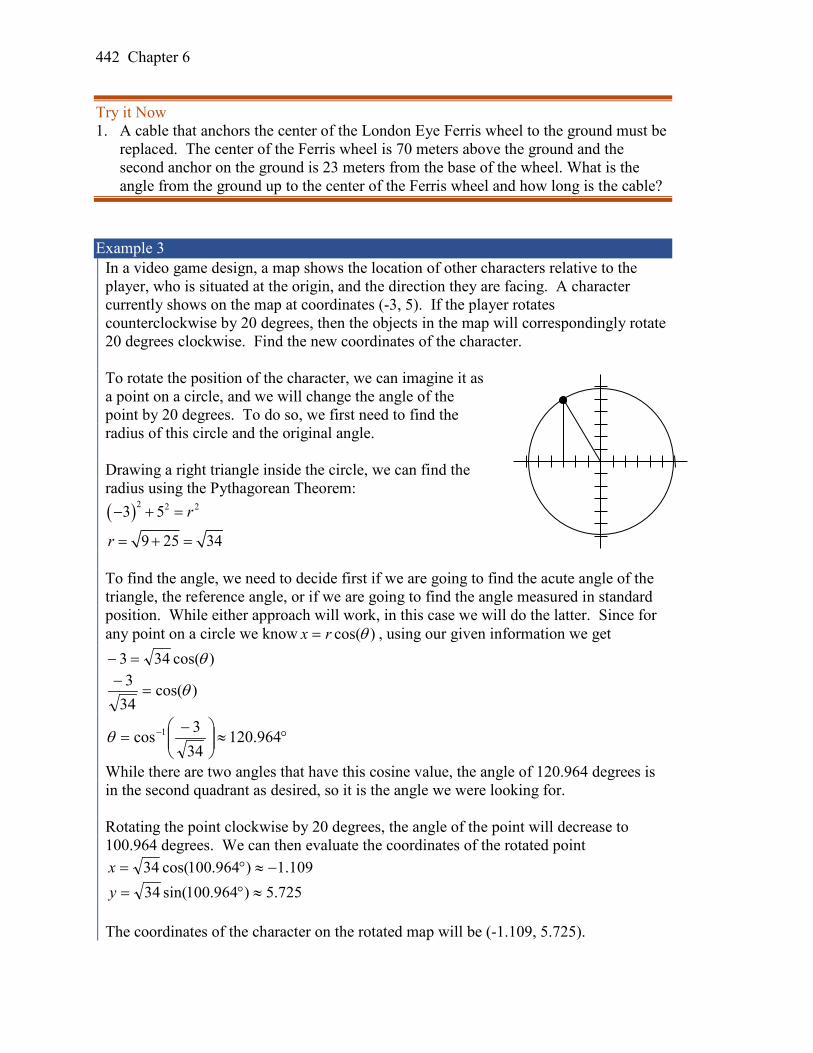
442 Chapter 6
Try it Now 1. A cable that anchors the center of the London Eye Ferris wheel to the ground must be
replaced. The center of the Ferris wheel is 70 meters above the ground and the second anchor on the ground is 23 meters from the base of the wheel. What is the angle from the ground up to the center of the Ferris wheel and how long is the cable?
Example 3
In a video game design, a map shows the location of other characters relative to the player, who is situated at the origin, and the direction they are facing. A character currently shows on the map at coordinates (-3, 5). If the player rotates counterclockwise by 20 degrees, then the objects in the map will correspondingly rotate 20 degrees clockwise. Find the new coordinates of the character. To rotate the position of the character, we can imagine it as a point on a circle, and we will change the angle of the point by 20 degrees. To do so, we first need to find the radius of this circle and the original angle. Drawing a right triangle inside the circle, we can find the radius using the Pythagorean Theorem: ( )2 2 23 5
9 25 34
r
r
− + =
= + =
To find the angle, we need to decide first if we are going to find the acute angle of the triangle, the reference angle, or if we are going to find the angle measured in standard position. While either approach will work, in this case we will do the latter. Since for any point on a circle we know )cos(θrx = , using our given information we get
)cos(343 θ=−
)cos(343 θ=
−
°≈
−= − 964.120
343cos 1θ
While there are two angles that have this cosine value, the angle of 120.964 degrees is in the second quadrant as desired, so it is the angle we were looking for. Rotating the point clockwise by 20 degrees, the angle of the point will decrease to 100.964 degrees. We can then evaluate the coordinates of the rotated point
The coordinates of the character on the rotated map will be (-1.109, 5.725).
109.1)964.100cos(34 −≈°=x725.5)964.100sin(34 ≈°=y

Section 6.5 Modeling with Trigonometric Functions 443
Modeling with sinusoidal functions Many modeling situations involve functions that are periodic. Previously we learned that sinusoidal functions are a special type of periodic function. Problems that involve quantities that oscillate can often be modeled by a sine or cosine function and once we create a suitable model for the problem we can use that model to answer various questions. Example 4
The hours of daylight in Seattle oscillate from a low of 8.5 hours in January to a high of 16 hours in July4. When should you plant a garden if you want to do it during a month where there are 14 hours of daylight? To model this, we first note that the hours of daylight oscillate with a period of 12
months. 212 6
B π π= = corresponds to the horizontal stretch, found by using the ratio of
the original period to the new period. With a low of 8.5 and a high of 16, the midline will be halfway between these values, at
25.122
5.816=
+ .
The amplitude will be half the difference between the highest and lowest values:
75.32
5.816=
− , or equivalently the
distance from the midline to the high or low value, 16-12.25=3.75. Letting January be t = 0, the graph starts at the lowest value, so it can be modeled as a flipped cosine graph. Putting this together, we get a model:
25.126
cos75.3)( +
−= tth π
h(t) is our model for hours of day light t months after January. To find when there will be 14 hours of daylight, we solve h(t) = 14.
25.126
cos75.314 +
−= tπ Isolating the cosine
4 http://www.mountaineers.org/seattle/climbing/Reference/DaylightHrs.html

444 Chapter 6
−= t
6cos75.375.1 π Subtracting 12.25 and dividing by -3.75
=− t
6cos
75.375.1 π Using the inverse
0563.275.375.1cos
61 ≈
−= −tπ multiplying by the reciprocal
927.360563.2 =⋅=π
t t=3.927 months past January
There will be 14 hours of daylight 3.927 months into the year, or near the end of April. While there would be a second time in the year when there are 14 hours of daylight, since we are planting a garden, we would want to know the first solution, in spring, so we do not need to find the second solution in this case.
Try it Now 2. The author’s monthly
gas usage (in therms) is shown here. Find a function to model the data.
Example 6
An object is connected to the wall with a spring that has a natural length of 20 cm. The object is pulled back 8 cm past the natural length and released. The object oscillates 3 times per second. Find an equation for the horizontal position of the object ignoring the effects of friction. How much time during each cycle is the object more than 27 cm from the wall? If we use the distance from the wall, x, as the desired output, then the object will oscillate equally on either side of the spring’s natural length of 20, putting the midline of the function at 20 cm. If we release the object 8 cm past the natural length, the amplitude of the oscillation will be 8 cm. We are beginning at the largest value and so this function can most easily be modeled using a cosine function.
020406080100120140160
Jan Feb Mar Apr May Jun Jul Aug Sep Oct Nov Dec

Section 6.5 Modeling with Trigonometric Functions 445
Since the object oscillates 3 times per second, it has a frequency of 3 and the period of one oscillation is 1/3 of second. Using this we find the horizontal compression using the
ratios of the periods: ππ 63/1
2= .
Using all this, we can build our model:
( ) 206cos8)( += ttx π To find when the object is 27 cm from the wall, we can solve x(t) = 27
( ) 206cos827 += tπ Isolating the cosine ( )tπ6cos87 =
( )tπ6cos87= Using the inverse
505.087cos6 1 ≈
= −tπ
0268.06505.0
==π
t
Based on the shape of the graph, we can conclude that the object will spend the first 0.0268 seconds more than 27 cm from the wall. Based on the symmetry of the function, the object will spend another 0.0268 seconds more than 27 cm from the wall at the end of the cycle. Altogether, the object spends 0.0536 seconds each cycle at a distance greater than 27 cm from the wall.
In some problems, we can use trigonometric functions to model behaviors more complicated than the basic sinusoidal function. Example 7
A rigid rod with length 10 cm is attached to a circle of radius 4cm at point A as shown here. The point B is able to freely move along the horizontal axis, driving a piston5. If the wheel rotates counterclockwise at 5 revolutions per second, find the location of point B as a function of time. When will the point B be 12 cm from the center of the circle?
5 For an animation of this situation, see http://www.mathdemos.org/mathdemos/sinusoidapp/engine1.gif
A
B 10 cm 4cm
θ

446 Chapter 6
To find the position of point B, we can begin by finding the coordinates of point A. Since it is a point on a circle with radius 4, we can express its coordinates as
))sin(4),cos(4( θθ , where θ is the angle shown. The angular velocity is 5 revolutions per second, or equivalently 10π radians per second. After t seconds, the wheel will rotate by 10 tθ π= radians. Substituting this, we can find the coordinates of A in terms of t.
))10sin(4),10cos(4( tt ππ Notice that this is the same value we would have obtained by observing that the period of the rotation is 1/5 of a second and calculating the stretch/compression factor:
ππ 105
12
""""
=new
original .
Now that we have the coordinates of the point A, we can relate this to the point B. By drawing a vertical line segment from A to the horizontal axis, we can form a right triangle. The height of the triangle is the y coordinate of the point A: 4sin(10 )tπ . Using the Pythagorean Theorem, we can find the base length of the triangle: ( )2 2 24sin(10 ) 10t bπ + =
2 2100 16sin (10 )b tπ= − 2100 16sin (10 )b tπ= −
Looking at the x coordinate of the point A, we can see that the triangle we drew is shifted to the right of the y axis by 4cos(10 )tπ . Combining this offset with the length of the base of the triangle gives the x coordinate of the point B:
2( ) 4cos(10 ) 100 16sin (10 )x t t tπ π= + − To solve for when the point B will be 12 cm from the center of the circle, we need to solve x(t) = 12.
212 4cos(10 ) 100 16sin (10 )t tπ π= + − Isolate the square root 212 4cos(10 ) 100 16sin (10 )t tπ π− = − Square both sides
( )2 212 4cos(10 ) 100 16sin (10 )t tπ π− = − Expand the left side 2 2144 96cos(10 ) 16cos (10 ) 100 16sin (10 )t t tπ π π− + = − Move all terms to the left
2 244 96cos(10 ) 16cos (10 ) 16sin (10 ) 0t t tπ π π− + + = Factor out 16
( )2 244 96cos(10 ) 16 cos (10 ) sin (10 ) 0t t tπ π π− + + =
A
B 10 cm
b

Section 6.5 Modeling with Trigonometric Functions 447
At this point, we can utilize the Pythagorean Identity, which tells us that 2 2cos (10 ) sin (10 ) 1t tπ π+ = .
Using this identity, our equation simplifies to 44 96cos(10 ) 16 0tπ− + = Combine the constants and move to the right side
96cos(10 ) 60tπ− = − Divide 60cos(10 )96
tπ = Make a substitution
9660)cos( =u
896.09660cos 1 ≈
= −u By symmetry we can find a second solution
388.5896.02 =−= πu Undoing the substitution 10 0.896tπ = , so t = 0.0285 10 5.388tπ = , so t = 0.1715 The point B will be 12 cm from the center of the circle 0.0285 seconds after the process begins, 0.1715 seconds after the process begins, and every 1/5 of a second after each of those values.
Important Topics of This Section Modeling with trig equations Modeling with sinusoidal functions Solving right triangles for angles in degrees and radians
Try it Now Answers 1. Angle of elevation for the cable is 71.81 degrees and the cable is 73.68 m long
2. Approximately ( ) 66cos ( 1) 876
G t tπ = − +

448 Chapter 6
Section 6.5 Exercises In each of the following triangles, solve for the unknown side and angles. 1. 2. 3. 4.
Find a possible formula for the trigonometric function whose values are in the following tables.
5. x 0 1 2 3 4 5 6 y -2 4 10 4 -2 4 10
6.
x 0 1 2 3 4 5 6 y 1 -3 -7 -3 1 -3 -7
7. Outside temperature over the course of a day can be modeled as a sinusoidal function.
Suppose you know the high temperature for the day is 63 degrees and the low temperature of 37 degrees occurs at 5 AM. Assuming t is the number of hours since midnight, find an equation for the temperature, D, in terms of t.
8. Outside temperature over the course of a day can be modeled as a sinusoidal function. Suppose you know the high temperature for the day is 92 degrees and the low temperature of 78 degrees occurs at 4 AM. Assuming t is the number of hours since midnight, find an equation for the temperature, D, in terms of t.
9. A population of rabbits oscillates 25 above and below an average of 129 during the year, hitting the lowest value in January (t = 0).
a. Find an equation for the population, P, in terms of the months since January, t. b. What if the lowest value of the rabbit population occurred in April instead?
A 5
8
B c
B
7
3
A
c
A
b
7 15 B
B
a 10
12 A

Section 6.5 Modeling with Trigonometric Functions 449
10. A population of elk oscillates 150 above and below an average of 720 during the year, hitting the lowest value in January (t = 0).
a. Find an equation for the population, P, in terms of the months since January, t. b. What if the lowest value of the rabbit population occurred in March instead?
11. Outside temperature over the course of a day can be modeled as a sinusoidal function. Suppose you know the high temperature of 105 degrees occurs at 5 PM and the average temperature for the day is 85 degrees. Find the temperature, to the nearest degree, at 9 AM.
12. Outside temperature over the course of a day can be modeled as a sinusoidal function. Suppose you know the high temperature of 84 degrees occurs at 6 PM and the average temperature for the day is 70 degrees. Find the temperature, to the nearest degree, at 7 AM.
13. Outside temperature over the course of a day can be modeled as a sinusoidal function. Suppose you know the temperature varies between 47 and 63 degrees during the day and the average daily temperature first occurs at 10 AM. How many hours after midnight does the temperature first reach 51 degrees?
14. Outside temperature over the course of a day can be modeled as a sinusoidal function.
Suppose you know the temperature varies between 64 and 86 degrees during the day and the average daily temperature first occurs at 12 AM. How many hours after midnight does the temperature first reach 70 degrees?
15. A Ferris wheel is 20 meters in diameter and boarded from a platform that is 2 meters
above the ground. The six o'clock position on the Ferris wheel is level with the loading platform. The wheel completes 1 full revolution in 6 minutes. How many minutes of the ride are spent higher than 13 meters above the ground?
16. A Ferris wheel is 45 meters in diameter and boarded from a platform that is 1 meter
above the ground. The six o'clock position on the Ferris wheel is level with the loading platform. The wheel completes 1 full revolution in 10 minutes. How many minutes of the ride are spent higher than 27 meters above the ground?
17. The sea ice area around the North Pole fluctuates between about 6 million square kilometers in September to 14 million square kilometers in March. Assuming sinusoidal fluctuation, during how many months are there less than 9 million square kilometers of sea ice?
18. The sea ice area around the South Pole fluctuates between about 18 million square kilometers in September to 3 million square kilometers in March. Assuming sinusoidal fluctuation, during how many months are there more than 15 million square kilometers of sea ice?

450 Chapter 6
19. A respiratory ailment called “Cheyne-Stokes Respiration” causes the volume per breath to increase and decrease in a sinusoidal manner, as a function of time. For one particular patient with this condition, a machine begins recording a plot of volume per breath versus time (in seconds). Let ( )b t be a function of time t that tells us the volume (in liters) of a breath that starts at time t. During the test, the smallest volume per breath is 0.6 liters and this first occurs for a breath that starts 5 seconds into the test. The largest volume per breath is 1.8 liters and this first occurs for a breath beginning 55 seconds into the test. [UW] a. Find a formula for the function ( )b t whose graph will model the test data for this
patient. b. If the patient begins a breath every 5 seconds, what are the breath volumes during
the first minute of the test?
20. Suppose the high tide in Seattle occurs at 1:00 a.m. and 1:00 p.m, at which time the water is 10 feet above the height of low tide. Low tides occur 6 hours after high tides. Suppose there are two high tides and two low tides every day and the height of the tide varies sinusoidally. [UW] a. Find a formula for the function ( )y h t= that computes the height of the tide above
low tide at time t. (In other words, y = 0 corresponds to low tide.) b. What is the tide height at 11:00 a.m.?
21. A communications satellite orbits the earth t
miles above the surface. Assume the radius of the earth is 3,960 miles. The satellite can only “see” a portion of the earth’s surface, bounded by what is called a horizon circle. This leads to a two-dimensional cross-sectional picture we can use to study the size of the horizon slice: [UW] a. Find a formula for α in terms of t. b. If t = 30,000 miles, what is α? What
percentage of the circumference of the earth is covered by the satellite? What would be the minimum number of such satellites required to cover the circumference?
c. If t = 1,000 miles, what is α? What percentage of the circumference of the earth is covered by the satellite? What would be the minimum number of such satellites required to cover the circumference?
d. Suppose you wish to place a satellite into orbit so that 20% of the circumference is covered by the satellite. What is the required distance t?

Section 6.5 Modeling with Trigonometric Functions 451
22. Tiffany is a model rocket enthusiast. She has been working on a pressurized rocket filled with nitrous oxide. According to her design, if the atmospheric pressure exerted on the rocket is less than 10 pounds/sq.in., the nitrous oxide chamber inside the rocket will explode. Tiff worked from a formula /1014.7 hp e−= pounds/sq.in. for the atmospheric pressure h miles above sea level. Assume that the rocket is launched at an angle of α above level ground at sea level with an initial speed of 1400 feet/sec. Also, assume the height (in feet) of the rocket at time t seconds is given by the equation ( ) ( )216 1400siny t t tα= − + . [UW] a. At what altitude will the rocket explode? b. If the angle of launch is α = 12°, determine the minimum atmospheric pressure
exerted on the rocket during its flight. Will the rocket explode in midair? c. If the angle of launch is α = 82°, determine the minimum atmospheric pressure
exerted on the rocket during its flight. Will the rocket explode in midair? d. Find the largest launch angle α so that the rocket will not explode.

452 Chapter 6

Section 7.1 Solving Trigonometric Equations and Identities 453
This chapter is part of Precalculus: An Investigation of Functions © Lippman & Rasmussen 2017. This material is licensed under a Creative Commons CC-BY-SA license.
Chapter 7: Trigonometric Equations and Identities In the last two chapters we have used basic definitions and relationships to simplify trigonometric expressions and solve trigonometric equations. In this chapter we will look at more complex relationships. By conducting a deeper study of trigonometric identities we can learn to simplify complicated expressions, allowing us to solve more interesting applications.
Section 7.1 Solving Trigonometric Equations with Identities .................................... 453 Section 7.2 Addition and Subtraction Identities ......................................................... 461 Section 7.3 Double Angle Identities ........................................................................... 477 Section 7.4 Modeling Changing Amplitude and Midline ........................................... 488
Section 7.1 Solving Trigonometric Equations with Identities In the last chapter, we solved basic trigonometric equations. In this section, we explore the techniques needed to solve more complicated trig equations. Building from what we already know makes this a much easier task. Consider the function 2( ) 2f x x x= + . If you were asked to solve 0)( =xf , it requires simple algebra:
02 2 =+ xx Factor 0)12( =+xx Giving solutions
x = 0 or x = 21
−
Similarly, for ( ) sin( )g t t= , if we asked you to solve 0)( =tg , you can solve this using unit circle values:
0)sin( =t for ππ 2,,0=t and so on. Using these same concepts, we consider the composition of these two functions:
)sin()(sin2))(sin())(sin(2))(( 22 tttttgf +=+= This creates an equation that is a polynomial trig function. With these types of functions, we use algebraic techniques like factoring and the quadratic formula, along with trigonometric identities and techniques, to solve equations. As a reminder, here are some of the essential trigonometric identities that we have learned so far:

454 Chapter 7
Identities Pythagorean Identities
1)(sin)(cos 22 =+ tt )(csc)(cot1 22 tt =+ )(sec)(tan1 22 tt =+ Negative Angle Identities
)sin()sin( tt −=− )cos()cos( tt =− )tan()tan( tt −=− )csc()csc( tt −=− )sec()sec( tt =− )cot()cot( tt −=−
Reciprocal Identities
)cos(1)sec(
tt =
)sin(1)csc(
tt =
)cos()sin()tan(
ttt =
)tan(1)cot(
tt =
Example 1
Solve 0)sin()(sin2 2 =+ tt for all solutions with π20 <≤ t . This equation kind of looks like a quadratic equation, but with sin(t) in place of an algebraic variable (we often call such an equation “quadratic in sine”). As with all quadratic equations, we can use factoring techniques or the quadratic formula. This expression factors nicely, so we proceed by factoring out the common factor of sin(t):
( ) 01)sin(2)sin( =+tt Using the zero product theorem, we know that the product on the left will equal zero if either factor is zero, allowing us to break this equation into two cases:
0)sin( =t or 01)sin(2 =+t We can solve each of these equations independently, using our knowledge of special angles.
0)sin( =t 01)sin(2 =+t
t = 0 or t = π 21)sin( −=t
6
7π=t or
611π
=t
Together, this gives us four solutions to the equation on π20 <≤ t :
611,
67,,0 πππ=t
We could check these answers are reasonable by graphing the function and comparing the zeros.

Section 7.1 Solving Trigonometric Equations and Identities 455
Example 2 Solve 02)sec(5)(sec3 2 =−− tt for all solutions with π20 <≤ t . Since the left side of this equation is quadratic in secant, we can try to factor it, and hope it factors nicely. If it is easier to for you to consider factoring without the trig function present, consider using a substitution )sec(tu = , resulting in 0253 2 =−− uu , and then try to factor:
)2)(13(253 2 −+=−− uuuu Undoing the substitution,
0)2))(sec(1)sec(3( =−+ tt Since we have a product equal to zero, we break it into the two cases and solve each separately.
01)sec(3 =+t Isolate the secant
31)sec( −=t Rewrite as a cosine
31
)cos(1
−=t
Invert both sides
3)cos( −=t Since the cosine has a range of [-1, 1], the cosine will never take on an output of -3. There are no solutions to this case. Continuing with the second case,
02)sec( =−t Isolate the secant 2)sec( =t Rewrite as a cosine
2)cos(
1=
t Invert both sides
21)cos( =t This gives two solutions
3π
=t or 3
5π=t
These are the only two solutions on the interval. By utilizing technology to graph
2( ) 3sec ( ) 5sec( ) 2f t t t= − − , a look at a graph confirms there are only two zeros for this function on the interval [0, 2π), which assures us that we didn’t miss anything.

456 Chapter 7
Try it Now 1. Solve 01)sin(3)(sin2 2 =++ tt for all solutions with π20 <≤ t .
When solving some trigonometric equations, it becomes necessary to first rewrite the equation using trigonometric identities. One of the most common is the Pythagorean Identity, 1)(cos)(sin 22 =+ θθ which allows you to rewrite )(sin 2 θ in terms of )(cos2 θ or vice versa,
Identities Alternate Forms of the Pythagorean Identity
2 2
2 2
sin ( ) 1 cos ( )cos ( ) 1 sin ( )
θ θ
θ θ
= −
= − These identities become very useful whenever an equation involves a combination of sine and cosine functions. Example 3
Solve 1)cos()(sin2 2 =− tt for all solutions with π20 <≤ t . Since this equation has a mix of sine and cosine functions, it becomes more complicated to solve. It is usually easier to work with an equation involving only one trig function. This is where we can use the Pythagorean Identity.
1)cos()(sin2 2 =− tt Using )(cos1)(sin 22 θθ −=
( ) 1)cos()(cos12 2 =−− tt Distributing the 2
1)cos()(cos22 2 =−− tt Since this is now quadratic in cosine, we rearrange the equation so one side is zero and factor.
01)cos()(cos2 2 =+−− tt Multiply by -1 to simplify the factoring
01)cos()(cos2 2 =−+ tt Factor ( )( ) 01)cos(1)cos(2 =+− tt This product will be zero if either factor is zero, so we can break this into two separate cases and solve each independently.

Section 7.1 Solving Trigonometric Equations and Identities 457
01)cos(2 =−t or 01)cos( =+t
21)cos( =t or 1)cos( −=t
3π
=t or 3
5π=t or π=t
Try it Now 2. Solve )cos(3)(sin2 2 tt = for all solutions with π20 <≤ t .
In addition to the Pythagorean Identity, it is often necessary to rewrite the tangent, secant, cosecant, and cotangent as part of solving an equation. Example 4
Solve )sin(3)tan( xx = for all solutions with π20 <≤ x . With a combination of tangent and sine, we might try rewriting tangent
)sin(3)tan( xx =
)sin(3)cos()sin( x
xx
= Multiplying both sides by cosine
)cos()sin(3)sin( xxx = At this point, you may be tempted to divide both sides of the equation by sin(x). Resist the urge. When we divide both sides of an equation by a quantity, we are assuming the quantity is never zero. In this case, when sin(x) = 0 the equation is satisfied, so we’d lose those solutions if we divided by the sine. To avoid this problem, we can rearrange the equation so that one side is zero1.
0)cos()sin(3)sin( =− xxx Factoring out sin(x) from both parts ( ) 0)cos(31)sin( =− xx
From here, we can see we get solutions when 0)sin( =x or 0)cos(31 =− x . Using our knowledge of the special angles of the unit circle,
0)sin( =x when x = 0 or x = π.
1 You technically can divide by sin(x), as long as you separately consider the case where sin(x) = 0. Since it is easy to forget this step, the factoring approach used in the example is recommended.
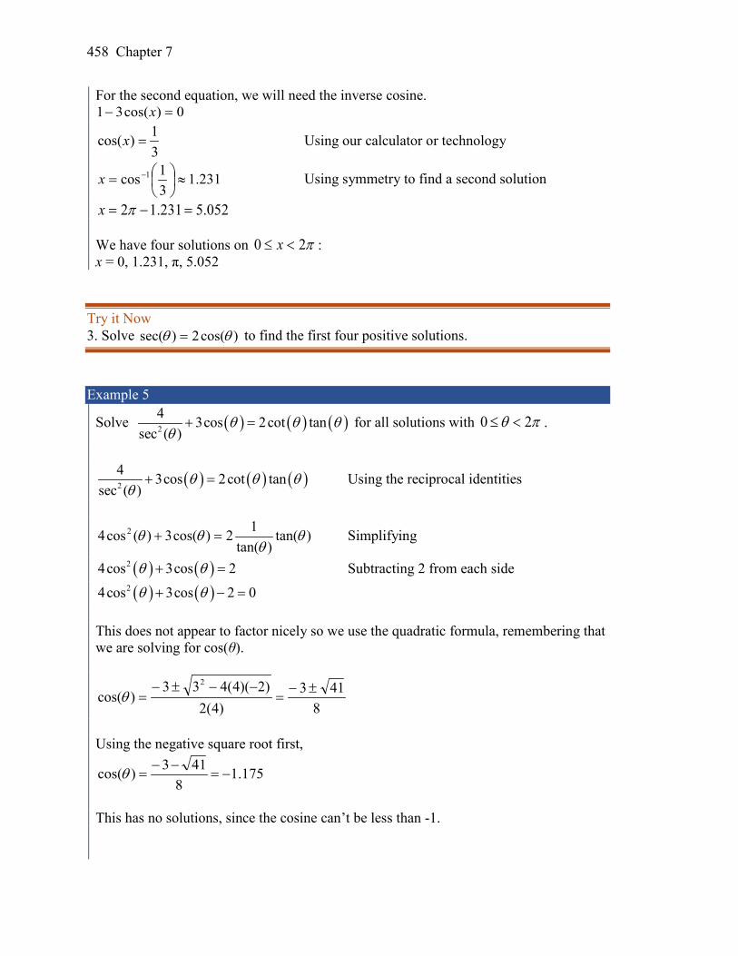
458 Chapter 7
For the second equation, we will need the inverse cosine. 0)cos(31 =− x
31)cos( =x Using our calculator or technology
231.131cos 1 ≈
= −x Using symmetry to find a second solution
052.5231.12 =−= πx We have four solutions on π20 <≤ x : x = 0, 1.231, π, 5.052
Try it Now 3. Solve )cos(2)sec( θθ = to find the first four positive solutions.
Example 5
Solve ( ) ( ) ( )2
4 3cos 2cot tansec ( )
θ θ θθ
+ = for all solutions with 0 2θ π≤ < .
( ) ( ) ( )2
4 3cos 2cot tansec ( )
θ θ θθ
+ = Using the reciprocal identities
)tan()tan(
12)cos(3)(cos4 2 θθ
θθ =+ Simplifying
( ) ( )24cos 3cos 2θ θ+ = Subtracting 2 from each side
( ) ( )24cos 3cos 2 0θ θ+ − = This does not appear to factor nicely so we use the quadratic formula, remembering that we are solving for cos(θ).
8413
)4(2)2)(4(433
)cos(2 ±−
=−−±−
=θ
Using the negative square root first,
175.18
413)cos( −=−−
=θ
This has no solutions, since the cosine can’t be less than -1.

Section 7.1 Solving Trigonometric Equations and Identities 459
Using the positive square root,
425.08
413)cos( =+−
=θ
( ) 131.1425.0cos 1 == −θ By symmetry, a second solution can be found 152.5131.12 =−= πθ
Important Topics of This Section Review of Trig Identities Solving Trig Equations By Factoring Using the Quadratic Formula Utilizing Trig Identities to simplify
Try it Now Answers 1. Factor as ( )( ) 01)sin(1)sin(2 =++ tt
01)sin(2 =+t at 7 11,6 6
t π π=
01)sin( =+t at 32
t π=
7 3 11, ,6 2 6
t π π π=
2. ( ) )cos(3)(cos12 2 tt =−
02)cos(3)(cos2 2 =−+ tt ( )( ) 02)cos(1)cos(2 =+− tt
02)cos( =+t has no solutions
01)cos(2 =−t at 5,3 3
t π π=
3. )cos(2)cos(
1 θθ
=
)(cos21 2 θ=
22
21)cos( ±=±=θ
3 5 7, , ,4 4 4 4π π π πθ =

460 Chapter 7
Section 7.1 Exercises Find all solutions on the interval 0 2θ π≤ < . 1. ( )2sin 1θ = − 2. ( )2sin 3θ = 3. ( )2cos 1θ = 4. ( )2cos 2θ =− Find all solutions.
5. 2sin 1 4
xπ =
6. 2sin 23
xπ =
7. ( )2cos 2 3t = − 8. ( )2cos 3 1t = −
9. 3cos 25
xπ =
10. 8cos 62
xπ =
11. ( )7sin 3 2t = − 12. ( )4sin 4 1t =
Find all solutions on the interval [0, 2 )π . 13. ( ) ( ) ( )10sin cos 6cosx x x= 14. ( ) ( ) ( )3sin 15cos sint t t− =
15. ( )csc 2 9 0x − = 16. ( )sec 2 3θ =
17. ( ) ( ) ( )sec sin 2sin 0x x x− = 18. ( ) ( ) ( )tan sin sin 0x x x− =
19. 2 1sin4
x = 20. 2 1cos2
θ =
21. 2sec 7x = 22. 2csc 3t =
23. 22sin 3sin 1 0w w+ + = 24. ( )28sin 6sin 1 0x x+ + =
25. ( )22cos cos 1t t+ = 26. ( ) ( )28cos 3 2cosθ θ= −
27. ( )24cos ( ) 4 15cosx x− = 28. ( ) 29sin 2 4sin ( )w w− =
29. ( ) ( )212sin cos 6 0t t+ − = 30. ( ) ( )26cos 7sin 8 0x x+ − =
31. 2cos 6sinφ φ= − 32. 2sin cost t=
33. ( ) ( )3tan 3tanx x= 34. ( ) ( )3cos cost t= −
35. ( ) ( )5tan tanx x= 36. ( ) ( )5tan 9 tan 0x x− =
37. ( ) ( ) ( ) ( )4sin cos 2sin 2cos 1 0x x x x+ − − =
38. ( ) ( ) ( ) ( )2sin cos sin 2cos 1 0x x x x− + − =
39. ( ) ( )tan 3sin 0x x− = 40. ( ) ( )3cos cotx x=
41. ( ) ( )22 tan 3sect t= 42. ( ) ( )21 2 tan tanw w− =

Section 7.2 Addition and Subtraction Identities 461
Section 7.2 Addition and Subtraction Identities In this section, we begin expanding our repertoire of trigonometric identities.
Identities The sum and difference identities
)sin()sin()cos()cos()cos( βαβαβα +=−
)sin()sin()cos()cos()cos( βαβαβα −=+
)sin()cos()cos()sin()sin( βαβαβα +=+
)sin()cos()cos()sin()sin( βαβαβα −=−
We will prove the difference of angles identity for cosine. The rest of the identities can be derived from this one. Proof of the difference of angles identity for cosine Consider two points on a unit circle: P at an angle of α from the positive x axis with coordinates ( ))sin(),cos( αα , and Q at an angle of β with coordinates ( ))sin(),cos( ββ . Notice the measure of angle POQ is α – β. Label two more points: C at an angle of α – β, with coordinates ( ))sin(),cos( βαβα −− , D at the point (1, 0). Notice that the distance from C to D is the same as the distance from P to Q because triangle COD is a rotation of triangle POQ. Using the distance formula to find the distance from P to Q yields
( ) ( )22 )sin()sin()cos()cos( βαβα −+− Expanding this
)(sin)sin()sin(2)(sin)(cos)cos()cos(2)(cos 2222 ββααββαα +−++−
β α - β α
P
Q
C
D O

462 Chapter 7
Applying the Pythagorean Identity and simplifying
)sin()sin(2)cos()cos(22 βαβα −− Similarly, using the distance formula to find the distance from C to D
( ) ( )22 0)sin(1)cos( −−+−− βαβα Expanding this
)(sin1)cos(2)(cos 22 βαβαβα −++−−− Applying the Pythagorean Identity and simplifying
2)cos(2 +−− βα Since the two distances are the same we set these two formulas equal to each other and simplify
2)cos(2)sin()sin(2)cos()cos(22 +−−=−− βαβαβα 2)cos(2)sin()sin(2)cos()cos(22 +−−=−− βαβαβα
)cos()sin()sin()cos()cos( βαβαβα −=+ This establishes the identity. Try it Now 1. By writing )cos( βα + as ( )( )βα −−cos , show the sum of angles identity for cosine
follows from the difference of angles identity proven above. The sum and difference of angles identities are often used to rewrite expressions in other forms, or to rewrite an angle in terms of simpler angles. Example 1
Find the exact value of )75cos( ° . Since °+°=° 453075 , we can evaluate )75cos( ° as
)4530cos()75cos( °+°=° Apply the cosine sum of angles identity )45sin()30sin()45cos()30cos( °°−°°= Evaluate
22
21
22
23
⋅−⋅= Simply
426 −
=

Section 7.2 Addition and Subtraction Identities 463
Try it Now
2. Find the exact value of
12
sin π .
Example 2
Rewrite
−
4sin πx in terms of sin(x) and cos(x).
−
4sin πx Use the difference of angles identity for sine
= ( ) ( )
−
4sincos
4cossin ππ xx Evaluate the cosine and sine and rearrange
( ) ( )xx cos22sin
22
−=
Additionally, these identities can be used to simplify expressions or prove new identities Example 3
Prove )tan()tan()tan()tan(
)sin()sin(
baba
baba
−+
=−+
.
As with any identity, we need to first decide which side to begin with. Since the left side involves sum and difference of angles, we might start there
)sin()sin(
baba
−+
Apply the sum and difference of angle identities
)sin()cos()cos()sin()sin()cos()cos()sin(
babababa
−+
=
Since it is not immediately obvious how to proceed, we might start on the other side, and see if the path is more apparent.
)tan()tan()tan()tan(
baba
−+
Rewriting the tangents using the tangent identity

464 Chapter 7
)cos()sin(
)cos()sin(
)cos()sin(
)cos()sin(
bb
aa
bb
aa
−
+= Multiplying the top and bottom by cos(a)cos(b)
)cos()cos()cos()sin(
)cos()sin(
)cos()cos()cos()sin(
)cos()sin(
babb
aa
babb
aa
−
+
= Distributing and simplifying
)cos()sin()cos()sin()cos()sin()cos()sin(
abbaabba
−+
= From above, we recognize this
)sin()sin(
baba
−+
= Establishing the identity
These identities can also be used to solve equations. Example 4
Solve 23)2cos()cos()2sin()sin( =+ xxxx .
By recognizing the left side of the equation as the result of the difference of angles identity for cosine, we can simplify the equation
23)2cos()cos()2sin()sin( =+ xxxx Apply the difference of angles identity
23)2cos( =− xx
23)cos( =−x Use the negative angle identity
23)cos( =x
Since this is a special cosine value we recognize from the unit circle, we can quickly write the answers:
kx
kx
ππ
ππ
26
11
26
+=
+=, where k is an integer

Section 7.2 Addition and Subtraction Identities 465
Combining Waves of Equal Period A sinusoidal function of the form )sin()( CBxAxf += can be rewritten using the sum of angles identity. Example 5
Rewrite
+=
33sin4)( πxxf as a sum of sine and cosine.
+
33sin4 πx Using the sum of angles identity
( ) ( )
+
=
3sin3cos
3cos3sin4 ππ xx Evaluate the sine and cosine
( ) ( )
⋅+⋅=
233cos
213sin4 xx Distribute and simplify
( ) ( )xx 3cos323sin2 += Notice that the result is a stretch of the sine added to a different stretch of the cosine, but both have the same horizontal compression, which results in the same period. We might ask now whether this process can be reversed – can a combination of a sine and cosine of the same period be written as a single sinusoidal function? To explore this, we will look in general at the procedure used in the example above.
)sin()( CBxAxf += Use the sum of angles identity ( ))sin()cos()cos()sin( CBxCBxA += Distribute the A
)sin()cos()cos()sin( CBxACBxA += Rearrange the terms a bit )cos()sin()sin()cos( BxCABxCA +=
Based on this result, if we have an expression of the form )cos()sin( BxnBxm + , we could rewrite it as a single sinusoidal function if we can find values A and C so that
)cos()sin( BxnBxm + )cos()sin()sin()cos( BxCABxCA += , which will require that:
)sin()cos(
CAnCAm
==
which can be rewritten as )sin(
)cos(
CAn
CAm
=
=
To find A,

466 Chapter 7
( ) ( )2222 )sin()cos( CACAnm +=+ )(sin)(cos 2222 CACA +=
( ))(sin)(cos 222 CCA += Apply the Pythagorean Identity and simplify 2A=
Rewriting a Sum of Sine and Cosine as a Single Sine To rewrite )cos()sin( BxnBxm + as )sin( CBxA +
222 nmA += , AmC =)cos( , and
AnC =)sin(
You can use either of the last two equations to solve for possible values of C. Since there will usually be two possible solutions, we will need to look at both to determine which quadrant C is in and determine which solution for C satisfies both equations.
Example 6
Rewrite )2cos(4)2sin(34 xx − as a single sinusoidal function.
Using the formulas above, ( ) ( ) 6416316434 222 =+⋅=−+=A , so A = 8. Solving for C,
23
834)cos( ==C , so
6π
=C or 6
11π=C .
However, notice 21
84)sin( −=
−=C . Sine is negative in the third and fourth quadrant,
so the angle that works for both is 6
11π=C .
Combining these results gives us the expression
+
6112sin8 πx
Try it Now 3. Rewrite )5cos(23)5sin(23 xx +− as a single sinusoidal function.
Rewriting a combination of sine and cosine of equal periods as a single sinusoidal function provides an approach for solving some equations.

Section 7.2 Addition and Subtraction Identities 467
Example 7 Solve 1)2cos(4)2sin(3 =+ xx to find two positive solutions. Since the sine and cosine have the same period, we can rewrite them as a single sinusoidal function.
( ) ( ) 2543 222 =+=A , so A = 5
53)cos( =C , so 927.0
53cos 1 ≈
= −C or 356.5927.02 =−= πC
Since 54)sin( =C , a positive value, we need the angle in the first quadrant, C = 0.927.
Using this, our equation becomes
( ) 1927.02sin5 =+x Divide by 5
( )51927.02sin =+x Make the substitution u = 2x + 0.927
( )51sin =u The inverse gives a first solution
201.051sin 1 ≈
= −u By symmetry, the second solution is
940.2201.0 =−= πu A third solution would be 485.6201.02 =+= πu
Undoing the substitution, we can find two positive solutions for x.
201.0927.02 =+x or 940.2927.02 =+x or 485.6927.02 =+x 726.02 −=x 013.22 =x 558.52 =x
363.0−=x 007.1=x 779.2=x Since the first of these is negative, we eliminate it and keep the two positive solutions,
007.1=x and 779.2=x .

468 Chapter 7
The Product-to-Sum and Sum-to-Product Identities
Identities The Product-to-Sum Identities
( )
( )
( ))cos()cos(21)cos()cos(
)cos()cos(21)sin()sin(
)sin()sin(21)cos()sin(
βαβαβα
βαβαβα
βαβαβα
−++=
+−−=
−++=
We will prove the first of these, using the sum and difference of angles identities from the beginning of the section. The proofs of the other two identities are similar and are left as an exercise. Proof of the product-to-sum identity for sin(α)cos(β) Recall the sum and difference of angles identities from earlier
)sin()cos()cos()sin()sin( βαβαβα +=+ )sin()cos()cos()sin()sin( βαβαβα −=−
Adding these two equations, we obtain
)cos()sin(2)sin()sin( βαβαβα =−++ Dividing by 2, we establish the identity
( ))sin()sin(21)cos()sin( βαβαβα −++=
Example 8
Write )4sin()2sin( tt as a sum or difference. Using the product-to-sum identity for a product of sines
( ))42cos()42cos(21)4sin()2sin( tttttt +−−=
( ))6cos()2cos(21 tt −−= If desired, apply the negative angle identity
( ))6cos()2cos(21 tt −= Distribute
)6cos(21)2cos(
21 tt −=

Section 7.2 Addition and Subtraction Identities 469
Try it Now
4. Evaluate
12cos
1211cos ππ .
Identities The Sum-to-Product Identities
( ) ( )
−
+
=+2
cos2
sin2sinsin vuvuvu
( ) ( )
+
−
=−2
cos2
sin2sinsin vuvuvu
( ) ( )
−
+
=+2
cos2
cos2coscos vuvuvu
( ) ( )
−
+
−=−2
sin2
sin2coscos vuvuvu
We will again prove one of these and leave the rest as an exercise. Proof of the sum-to-product identity for sine functions We define two new variables:
βαβα
−=+=
vu
Adding these equations yields α2=+ vu , giving 2
vu +=α
Subtracting the equations yields β2=− vu , or 2
vu −=β
Substituting these expressions into the product-to-sum identity
( ))sin()sin(21)cos()sin( βαβαβα −++= gives
( ) ( )( )vuvuvu sinsin21
2cos
2sin +=
−
+ Multiply by 2 on both sides
( ) ( )vuvuvu sinsin2
cos2
sin2 +=
−
+ Establishing the identity

470 Chapter 7
Try it Now 5. Notice that, using the negative angle identity, ( ) ( ) )sin()sin(sinsin vuvu −+=− . Use
this along with the sum of sines identity to prove the sum-to-product identity for ( ) ( )vu sinsin − .
Example 9
Evaluate )75cos()15cos( °−° . Using the sum-to-product identity for the difference of cosines,
)75cos()15cos( °−°
°−°
°+°
−=2
7515sin2
7515sin2 Simplify
( ) ( )°−°−= 30sin45sin2 Evaluate
22
21
222 =
−⋅⋅−=
Example 10
Prove the identity )tan()2sin()4sin()2cos()4cos( t
tttt
−=+− .
Since the left side seems more complicated, we can start there and simplify.
)2sin()4sin()2cos()4cos(
tttt
+− Use the sum-to-product identities
−
+
−
+
−=
224cos
224sin2
224sin
224sin2
tttt
tttt
Simplify
( ) ( )( ) ( )tt
ttcos3sin2sin3sin2−
= Simplify further
( )( )t
tcossin−
= Rewrite as a tangent
)tan(t−= Establishing the identity

Section 7.2 Addition and Subtraction Identities 471
Example 11 Solve ( ) ( )sin sin 3 cos( )t t tπ π π+ = for all solutions with 20 <≤ t . In an equation like th is, it is not immediately obvious how to proceed. One option would be to combine the two sine functions on the left side of the equation. Another would be to move the cosine to the left side of the equation, and combine it with one of the sines. For no particularly good reason, we’ll begin by combining the sines on the left side of the equation and see how things work out.
( ) ( )sin sin 3 cos( )t t tπ π π+ = Apply the sum to product identity on the left
3 32sin cos cos( )2 2
t t t t tπ π π π π+ − =
Simplify
( ) ( )2sin 2 cos cos( )t t tπ π π− = Apply the negative angle identity
( ) ( )2sin 2 cos cos( )t t tπ π π= Rearrange the equation to be 0 on one side
( ) ( )2sin 2 cos cos( ) 0t t tπ π π− = Factor out the cosine
( ) ( )( )cos 2sin 2 1 0t tπ π − = Using the Zero Product Theorem we know that at least one of the two factors must be
zero. The first factor, ( )cos tπ , has period 22==
ππP , so the solution interval of
20 <≤ t represents one full cycle of this function.
( )cos 0tπ = Substitute u tπ= ( ) 0cos =u On one cycle, this has solutions
2π
=u or 2
3π=u Undo the substitution
2t ππ = , so
21
=t
32
t ππ = , so 23
=t
The second factor, ( )2sin 2 1tπ − , has period of 122
==ππP , so the solution interval
20 <≤ t contains two complete cycles of this function.
( )2sin 2 1 0tπ − = Isolate the sine
( ) 1sin 22
tπ = Substitute 2u tπ=

472 Chapter 7
21)sin( =u On one cycle, this has solutions
6π
=u or 6
5π=u On the second cycle, the solutions are
613
62 πππ =+=u or
617
652 πππ =+=u Undo the substitution
26
t ππ = , so 121
=t
526
t ππ = , so 125
=t
1326
t ππ = , so 1213
=t
1726
t ππ = , so 1217
=t
Altogether, we found six solutions on
20 <≤ t , which we can confirm by looking at the graph.
1217,
23,
1213,
21,
125,
121
=t
Important Topics of This Section The sum and difference identities Combining waves of equal periods Product-to-sum identities Sum-to-product identities Completing proofs
Try it Now Answers
1.
)sin()sin()cos()cos())sin()(sin()cos()cos()sin()sin()cos()cos(
))(cos()cos(
βαβαβαβαβαβα
βαβα
−−+
−+−−−=+

Section 7.2 Addition and Subtraction Identities 473
2.
−
=
−=
4sin
3cos
4cos
3sin
43sin
12sin πππππππ
22
21
22
23
−=4
26 −
3. ( ) ( ) 362323222 =+−=A . A = 6
22
623)cos( −=
−=C ,
22
623)sin( ==C .
43π
=C
+
435sin6 πx
4.
−+
+=
121211cos
121211cos
21
12cos
1211cos ππππππ
( )
−−=
+=
231
21
65coscos
21 ππ
=4
32 −−
5. )sin()sin( vu − Use negative angle identity for sine
Use sum-to-product identity for sine
Eliminate the parenthesis
Establishing the identity
)sin()sin( vu −+
( ) ( )
−−
−+
2cos
2sin2 vuvu
+
−
2cos
2sin2 vuvu

474 Chapter 7
Section 7.2 Exercises Find an exact value for each of the following. 1. ( )sin 75° 2. ( )sin 195° 3. cos(165 )° 4. cos(345 )°
5. 7cos12π
6. cos12π
7. 5sin12π
8. 11sin12π
Rewrite in terms of ( )sin x and ( )cos x .
9. 11sin6
x π +
10. 3sin4
x π −
11. 5cos6
x π −
12. 2cos3
x π +
Simplify each expression.
13. csc 2
tπ −
14. sec2
wπ −
15. cot2
xπ −
16. tan2
xπ −
Rewrite the product as a sum. 17. ( ) ( )16sin 16 sin 11x x 18. ( ) ( )20cos 36 cos 6t t 19. ( ) ( )2sin 5 cos 3x x 20. ( ) ( )10cos 5 sin 10x x Rewrite the sum as a product. 21. ( ) ( )cos 6 cos 4t t+ 22. ( ) ( )cos 6 cos 4u u+ 23. ( ) ( )sin 3 sin 7x x+ 24. ( ) ( )sin sin 3h h+
25. Given ( ) 2sin3
a = and ( ) 1cos4
b = − , with a and b both in the interval ,2π π
:
a. Find ( )sin a b+ b. Find ( )cos a b−
26. Given ( ) 4sin5
a = and ( ) 1cos3
b = , with a and b both in the interval 0,2π
:
a. Find ( )sin a b− b. Find ( )cos a b+ Solve each equation for all solutions. 27. ( ) ( ) ( ) ( )sin 3 cos 6 cos 3 sin 6 0.9x x x x− =− 28. ( ) ( ) ( ) ( )sin 6 cos 11 cos 6 sin 11 0.1x x x x− =− 29. ( ) ( ) ( ) ( )cos 2 cos sin 2 sin 1x x x x+ =
30. ( ) ( ) ( ) ( ) 3cos 5 cos 3 sin 5 sin 32
x x x x− =
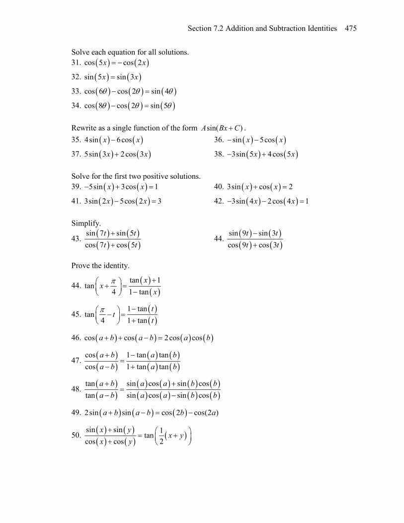
Section 7.2 Addition and Subtraction Identities 475
Solve each equation for all solutions. 31. ( ) ( )cos 5 cos 2x x= −
32. ( ) ( )sin 5 sin 3x x=
33. ( ) ( ) ( )cos 6 cos 2 sin 4θ θ θ− =
34. ( ) ( ) ( )cos 8 cos 2 sin 5θ θ θ− =
Rewrite as a single function of the form sin( ) A Bx C+ . 35. ( ) ( )4sin 6cosx x− 36. ( ) ( )sin 5cosx x− −
37. ( ) ( )5sin 3 2cos 3x x+ 38. ( ) ( )3sin 5 4cos 5x x− +
Solve for the first two positive solutions. 39. ( ) ( )5sin 3cos 1x x− + = 40. ( ) ( )3sin cos 2x x+ =
41. ( ) ( )3sin 2 5cos 2 3x x− = 42. ( ) ( )3sin 4 2cos 4 1x x− − =
Simplify.
43. ( ) ( )( ) ( )
sin 7 sin 5cos 7 cos 5
t tt t++
44. ( ) ( )( ) ( )
sin 9 sin 3cos 9 cos 3
t tt t−+
Prove the identity.
44. ( )( )
tan 1tan
4 1 tanx
xx
π + + = −
45. ( )( )
1 tantan
4 1 tant
tt
π − − = +
46. ( ) ( ) ( ) ( )cos cos 2cos cosa b a b a b+ + − =
47. ( )( )
( ) ( )( ) ( )
cos 1 tan tancos 1 tan tan
a b a ba b a b+ −
=− +
48. ( )( )
( ) ( ) ( ) ( )( ) ( ) ( ) ( )
tan sin cos sin costan sin cos sin cos
a b a a b ba b a a b b+ +
=− −
49. ( ) ( ) ( )2sin sin cos 2 cos(2 )a b a b b a+ − = −
50. ( ) ( )( ) ( ) ( )sin sin 1tan
cos cos 2x y
x yx y+ = + +

476 Chapter 7
Prove the identity.
51. ( )( ) ( ) ( ) ( )cos
1 tan tancos cos
a ba b
a b+
= −
52. ( ) ( ) 2 2cos cos cos sinx y x y x y+ − = −
53. Use the sum and difference identities to establish the product-to-sum identity
( ))cos()cos(21)sin()sin( βαβαβα +−−=
54. Use the sum and difference identities to establish the product-to-sum identity
( ))cos()cos(21)cos()cos( βαβαβα −++=
55. Use the product-to-sum identities to establish the sum-to-product identity
( ) ( )
−
+
=+2
cos2
cos2coscos vuvuvu
56. Use the product-to-sum identities to establish the sum-to-product identity
( ) ( )
−
+
−=−2
sin2
sin2coscos vuvuvu

Section 7.3 Double Angle Identities 477
Section 7.3 Double Angle Identities Two special cases of the sum of angles identities arise often enough that we choose to state these identities separately.
Identities The double angle identities
)cos()sin(2)2sin( ααα =
1)(cos2)(sin21
)(sin)(cos)2cos(
2
2
22
−=−=
−=
αα
ααα
These identities follow from the sum of angles identities. Proof of the sine double angle identity
)2sin( α )sin( αα += Apply the sum of angles identity
)sin()cos()cos()sin( αααα += Simplify )cos()sin(2 αα= Establishing the identity
Try it Now 1. Show )(sin)(cos)2cos( 22 ααα −= by using the sum of angles identity for cosine.
For the cosine double angle identity, there are three forms of the identity stated because the basic form, )(sin)(cos)2cos( 22 ααα −= , can be rewritten using the Pythagorean Identity. Rearranging the Pythagorean Identity results in the equality
)(sin1)(cos 22 αα −= , and by substituting this into the basic double angle identity, we obtain the second form of the double angle identity.
)(sin)(cos)2cos( 22 ααα −= Substituting using the Pythagorean identity )(sin)(sin1)2cos( 22 ααα −−= Simplifying
)(sin21)2cos( 2 αα −=

478 Chapter 7
Example 1
If 53)sin( =θ and θ is in the second quadrant, find exact values for )2sin( θ and
)2cos( θ . To evaluate )2cos( θ , since we know the value for sin( )θ we can use the version of the double angle that only involves sine.
257
25181
5321)(sin21)2cos(
22 =−=
−=−= θθ
Since the double angle for sine involves both sine and cosine, we’ll need to first find
)cos(θ , which we can do using the Pythagorean Identity. 1)(cos)(sin 22 =+ θθ
1)(cos53 2
2
=+
θ
2591)(cos2 −=θ
54
2516)cos( ±=±=θ
Since θ is in the second quadrant, we know that cos(θ) < 0, so
54)cos( −=θ
Now we can evaluate the sine double angle
2524
54
532)cos()sin(2)2sin( −=
−
== θθθ
Example 2
Simplify the expressions a) ( ) 112cos2 2 −° b) ( ) ( )xx 3cos3sin8 a) Notice that the expression is in the same form as one version of the double angle identity for cosine: 1)(cos2)2cos( 2 −= θθ . Using this,
( ) ( ) ( )°=°⋅=−° 24cos122cos112cos2 2 b) This expression looks similar to the result of the double angle identity for sine.
( ) ( )xx 3cos3sin8 Factoring a 4 out of the original expression ( ) ( )xx 3cos3sin24 ⋅ Applying the double angle identity )6sin(4 x

Section 7.3 Double Angle Identities 479
We can use the double angle identities to simplify expressions and prove identities. Example 2
Simplify )sin()cos(
)2cos(tt
t−
.
With three choices for how to rewrite the double angle, we need to consider which will be the most useful. To simplify this expression, it would be great if the denominator would cancel with something in the numerator, which would require a factor of
)sin()cos( tt − in the numerator, which is most likely to occur if we rewrite the numerator with a mix of sine and cosine.
)sin()cos()2cos(
ttt
− Apply the double angle identity
=)sin()cos(
)(sin)(cos 22
tttt
−− Factor the numerator
( )( ))sin()cos(
)sin()cos()sin()cos(tt
tttt−
+−= Cancelling the common factor
)sin()cos( tt += Resulting in the most simplified form Example 3
Prove )(sec2
)(sec)2sec( 2
2
ααα
−= .
Since the right side seems a bit more complicated than the left side, we begin there.
)(sec2)(sec
2
2
αα
− Rewrite the secants in terms of cosine
)(cos12
)(cos1
2
2
α
α
−=
At this point, we could rewrite the bottom with common denominators, subtract the terms, invert and multiply, then simplify. Alternatively, we can multiple both the top and bottom by )(cos2 α , the common denominator:
)(cos)(cos
12
)(cos)(cos
1
22
22
αα
αα
⋅
−
⋅= Distribute on the bottom

480 Chapter 7
⋅−=
)(cos)(cos)(cos2
)(cos)(cos
2
22
2
2
ααα
αα
Simplify
1)(cos21
2 −=
α Rewrite the denominator as a double angle
)2cos(1α
= Rewrite as a secant
)2sec( α= Establishing the identity Try it Now 2. Use an identity to find the exact value of ( ) ( )°−° 75sin75cos 22 .
As with other identities, we can also use the double angle identities for solving equations. Example 4
Solve )cos()2cos( tt = for all solutions with π20 <≤ t . In general when solving trig equations, it makes things more complicated when we have a mix of sines and cosines and when we have a mix of functions with different periods. In this case, we can use a double angle identity to rewrite the cos(2t). When choosing which form of the double angle identity to use, we notice that we have a cosine on the right side of the equation. We try to limit our equation to one trig function, which we can do by choosing the version of the double angle formula for cosine that only involves cosine.
)cos()2cos( tt = Apply the double angle identity )cos(1)(cos2 2 tt =− This is quadratic in cosine, so make one side 0
01)cos()(cos2 2 =−− tt Factor ( )( ) 01)cos(1)cos(2 =−+ tt Break this apart to solve each part separately
01)cos(2 =+t or 01)cos( =−t
21)cos( −=t or 1)cos( =t
32π
=t or 3
4π=t or 0=t
Looking at a graph of cos(2t) and cos(t) shown together, we can verify that these three
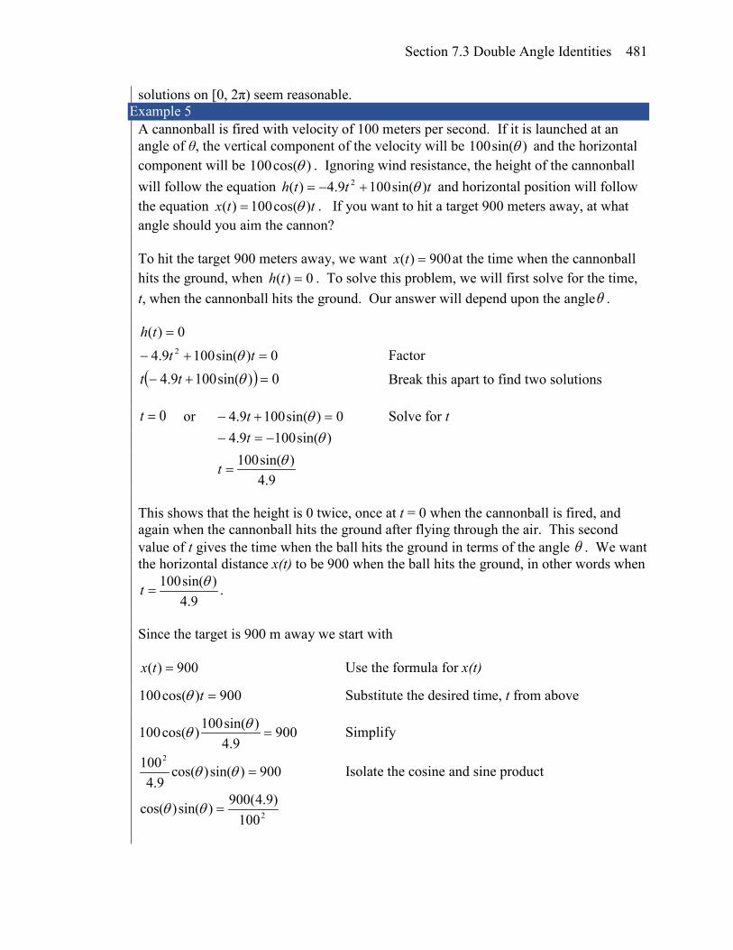
Section 7.3 Double Angle Identities 481
solutions on [0, 2π) seem reasonable. Example 5
A cannonball is fired with velocity of 100 meters per second. If it is launched at an angle of θ, the vertical component of the velocity will be )sin(100 θ and the horizontal component will be )cos(100 θ . Ignoring wind resistance, the height of the cannonball will follow the equation ttth )sin(1009.4)( 2 θ+−= and horizontal position will follow the equation ttx )cos(100)( θ= . If you want to hit a target 900 meters away, at what angle should you aim the cannon? To hit the target 900 meters away, we want 900)( =tx at the time when the cannonball hits the ground, when 0)( =th . To solve this problem, we will first solve for the time, t, when the cannonball hits the ground. Our answer will depend upon the angleθ .
0)( =th
0)sin(1009.4 2 =+− tt θ Factor
( ) 0)sin(1009.4 =+− θtt Break this apart to find two solutions
0=t or 0)sin(1009.4 =+− θt Solve for t )sin(1009.4 θ−=− t
9.4)sin(100 θ
=t
This shows that the height is 0 twice, once at t = 0 when the cannonball is fired, and again when the cannonball hits the ground after flying through the air. This second value of t gives the time when the ball hits the ground in terms of the angle θ . We want the horizontal distance x(t) to be 900 when the ball hits the ground, in other words when
9.4)sin(100 θ
=t .
Since the target is 900 m away we start with
900)( =tx Use the formula for x(t)
900)cos(100 =tθ Substitute the desired time, t from above
9009.4
)sin(100)cos(100 =θθ Simplify
900)sin()cos(9.4
1002
=θθ Isolate the cosine and sine product
2100)9.4(900)sin()cos( =θθ

482 Chapter 7
The left side of this equation almost looks like the result of the double angle identity for sine: ( ) ( )θθθ cossin2)2sin( = . Multiplying both sides of our equation by 2,
2100)9.4)(900(2)sin()cos(2 =θθ Using the double angle identity on the left
2100)9.4)(900(2)2sin( =θ Use the inverse sine
080.1100
)9.4)(900(2sin2 21 ≈
= −θ Divide by 2
540.02080.1
==θ , or about 30.94 degrees
Power Reduction and Half Angle Identities Another use of the cosine double angle identities is to use them in reverse to rewrite a squared sine or cosine in terms of the double angle. Starting with one form of the cosine double angle identity:
1)(cos2)2cos( 2 −= αα Isolate the cosine squared term )(cos21)2cos( 2 αα =+ Add 1
21)2cos()(cos2 +
=αα Divide by 2
21)2cos()(cos2 +
=αα This is called a power reduction identity
Try it Now 3. Use another form of the cosine double angle identity to prove the identity
2)2cos(1)(sin 2 αα −
= .
The cosine double angle identities can also be used in reverse for evaluating angles that
are half of a common angle. Building from our formula 2
1)2cos()(cos2 +=
αα , if we let
αθ 2= , then 2θα = this identity becomes
21)cos(
2cos2 +
=
θθ . Taking the square
root, we obtain
21)cos(
2cos +
±=
θθ , where the sign is determined by the quadrant.

Section 7.3 Double Angle Identities 483
This is called a half-angle identity. Try it Now 4. Use your results from the last Try it Now to prove the identity
2)cos(1
2sin θθ −
±=
.
Identities Half-Angle Identities
21)cos(
2cos +
±=
θθ
2)cos(1
2sin θθ −
±=
Power Reduction Identities
21)2cos()(cos2 +
=αα
2)2cos(1)(sin 2 αα −
=
Since these identities are easy to derive from the double-angle identities, the power reduction and half-angle identities are not ones you should need to memorize separately. Example 6
Rewrite )(cos4 x without any powers.
( )224 )(cos)(cos xx = Using the power reduction formula
2
21)2cos(
+
=x Square the numerator and denominator
( )2cos(2 ) 14x +
= Expand the numerator
41)2cos(2)2(cos2 ++
=xx Split apart the fraction
41
4)2cos(2
4)2(cos2
++=xx Apply the formula above to )2(cos2 x
2 cos(2 2 ) 1cos (2 )2
xx ⋅ +=

484 Chapter 7
41
4)2cos(2
42
1)4cos(
++
+
=x
x
Simplify
41)2cos(
21
81
8)4cos(
+++= xx Combine the constants
83)2cos(
21
8)4cos(
++= xx
Example 7
Find an exact value for ( )°15cos . Since 15 degrees is half of 30 degrees, we can use our result from above:
21)30cos(
230cos)15cos( +°
±=
°
=°
We can evaluate the cosine. Since 15 degrees is in the first quadrant, we need the positive result.
2
123
21)30cos( +=
+°
21
43+=
Important Topics of This Section Double angle identity Power reduction identity Half angle identity Using identities Simplify equations Prove identities Solve equations

Section 7.3 Double Angle Identities 485
Try it Now Answers
1. ( )
)(sin)(cos)sin()sin()cos()cos(
)cos(2cos
22 αα
ααααααα
−
−+=
2. ( ) ( ) )752cos(75sin75cos 22 °⋅=°−° = 2
3)150cos( −=°
3.
( )2 2
2 2
2 2
22
1 cos(2 )2
1 cos ( ) sin ( )2
1 cos ( ) sin ( )2
sin ( ) sin ( )2
2sin ( ) sin ( )2
α
α α
α α
α α
α α
−
− −
− +
+
=
4.
2)cos(1
2sin
22
2cos1
2sin
2
2)2cos(1)sin(
2)2cos(1)(sin 2
θθ
θθ
θα
αα
αα
−±=
−
±=
=
−±=
−=

486 Chapter 7
Section 7.3 Exercises
1. If ( ) 1sin8
x = and x is in quadrant I, then find exact values for (without solving for x):
a. ( )sin 2x b. ( )cos 2x c. ( )tan 2x
2. If ( ) 2cos3
x = and x is in quadrant I, then find exact values for (without solving for x):
a. ( )sin 2x b. ( )cos 2x c. ( )tan 2x Simplify each expression. 3. ( )2 2cos 28 sin (28 )° − ° 4. ( )22cos 37 1° − 5. 21 2sin (17 )− ° 6. ( )2 2cos 37 sin (37 )° − ° 7. ( )2 2cos 9 sin (9 )x x− 8. ( )2 2cos 6 sin (6 )x x− 9. ( )4sin 8 cos(8 )x x 10. ( )6sin 5 cos(5 )x x Solve for all solutions on the interval [0, 2 )π . 11. ( ) ( )6sin 2 9sin 0t t+ = 12. ( ) ( )2sin 2 3cos 0t t+ = 13. ( ) ( )29cos 2 9cos 4θ θ= − 14. ( ) ( )28cos 2 8cos 1α α= −
15. ( ) ( )sin 2 cost t= 16. ( ) ( )cos 2 sint t=
17. ( ) ( )cos 6 cos 3 0x x− = 18. ( ) ( )sin 4 sin 2 0x x− = Use a double angle, half angle, or power reduction formula to rewrite without exponents. 19. 2cos (5 )x 20. 2cos (6 )x 21. 4sin (8 )x 22. ( )4sin 3x 23. 2 4cos sinx x 24. 4 2cos sinx x
25. If ( )csc 7x = and 90 180x° < < ° , then find exact values for (without solving for x):
a. sin2x
b. cos2x
c. tan2x
26. If ( )sec 4x = and 270 360x° < < ° , then find exact values for (without solving for x):
a. sin2x
b. cos2x
c. tan2x
Prove the identity.

Section 7.3 Double Angle Identities 487
27. ( ) ( )2sin cos 1 sin 2t t t− = −
28. ( ) ( )22 4sin 1 cos 2 sinx x x− = +
29. ( ) ( )( )2
2 tansin 2
1 tanx
xx
=+
30. ( ) ( ) ( )( )2
2sin costan 2
2cos 1x x
xx
=−
31. ( ) ( ) ( )cot tan 2cot 2x x x− =
32. ( )( ) ( )sin 2
tan1 cos 2
θθ
θ=
+
33. ( ) ( )( )
2
2
1 tancos 2
1 tanα
αα
−=
+
34. ( )( ) ( )
( )( )
1 cos 2 2cossin 2 cos 2sin 1
t tt t t
+=
− −
35. ( ) ( ) ( )2 3sin 3 3sin cos sin ( )x x x x= −
36. ( ) ( )3 2cos 3 cos ( ) 3sin ( ) cosx x x x= −

488 Chapter 7
Section 7.4 Modeling Changing Amplitude and Midline While sinusoidal functions can model a variety of behaviors, it is often necessary to combine sinusoidal functions with linear and exponential curves to model real applications and behaviors. We begin this section by looking at changes to the midline of a sinusoidal function. Recall that the midline describes the middle, or average value, of the sinusoidal function. Changing Midlines Example 1
A population of elk currently averages 2000 elk, and that average has been growing by 4% each year. Due to seasonal fluctuation, the population oscillates from 50 below average in the winter up to 50 above average in the summer. Find a function that models the number of elk after t years, starting in the winter. There are two components to the behavior of the elk population: the changing average, and the oscillation. The average is an exponential growth, starting at 2000 and growing by 4% each year. Writing a formula for this:
(1 ) 2000(1 0.04)t taverage initial r= + = + For the oscillation, since the population oscillates 50 above and below average, the amplitude will be 50. Since it takes one year for the population to cycle, the period is 1.
We find the value of the horizontal stretch coefficient original period 2 2new period 1
B π π= = = .
The function starts in winter, so the shape of the function will be a negative cosine, since it starts at the lowest value. Putting it all together, the equation would be:
( ) 50cos(2 )P t t midlineπ= − + Since the midline represents the average population, we substitute in the exponential function into the population equation to find our final equation:
( ) 50cos(2 ) 2000(1 0.04)tP t tπ= − + + This is an example of changing midline – in this case an exponentially changing midline.

Section 7.4 Modeling Changing Amplitude and Midline 489
Changing Midline A function of the form )()sin()( tgBtAtf += will oscillate above and below the average given by the function g(t).
Changing midlines can be exponential, linear, or any other type of function. Here are some examples: Linear midline Exponential midline Quadratic midline
( )( ) sin ( )f t A Bt mt b= + + ( )( ) sin ( )tf t A Bt ab= + ( ) 2( ) sin ( )f t A Bt at= +
Example 2
Find a function with linear midline of the form bmttAtf ++
=
2sin)( π that will pass
through the points given below.
Since we are given the value of the horizontal compression coefficient we can calculate
the period of this function: original period 2new period 42Bπ
π= = = .
Since the sine function is at the midline at the beginning of a cycle and halfway through a cycle, we would expect this function to be at the midline at t = 0 and t = 2, since 2 is half the full period of 4. Based on this, we expect the points (0, 5) and (2, 9) to be points on the midline. We can clearly see that this is not a constant function and so we use the two points to calculate a linear function: bmtmidline += . From these two points we can calculate a slope:
224
0259
==−−
=m
Combining this with the initial value of 5, we have the midline: 52 += tmidline .
t 0 1 2 3 f(t) 5 10 9 8

490 Chapter 7
The full function will have form 522
sin)( ++
= ttAtf π . To find the amplitude, we
can plug in a point we haven’t already used, such as (1, 10).
5)1(2)1(2
sin10 ++
=πA Evaluate the sine and combine like terms
710 += A 3=A
A function of the form given fitting the data would be
522
sin3)( ++
= tttf π
Alternative Approach Notice we could have taken an alternate approach by plugging points (0, 5) and (2, 9) into the original equation. Substituting (0, 5),
bmA ++
= )0()0(
2sin5 π Evaluate the sine and simplify
b=5 Substituting (2, 9)
5)2()2(2
sin9 ++
= mA π Evaluate the sine and simplify
529 += m m24 = 2=m , as we found above. Now we can proceed to find A the same way we did before.
Example 3
The number of tourists visiting a ski and hiking resort averages 4000 people annually and oscillates seasonally, 1000 above and below the average. Due to a marketing campaign, the average number of tourists has been increasing by 200 each year. Write an equation for the number of tourists after t years, beginning at the peak season. Again there are two components to this problem: the oscillation and the average. For the oscillation, the number of tourists oscillates 1000 above and below average, giving an amplitude of 1000. Since the oscillation is seasonal, it has a period of 1 year. Since we are given a starting point of “peak season”, we will model this scenario with a cosine function. So far, this gives an equation in the form ( ) 1000cos(2 )N t t midlineπ= + .

Section 7.4 Modeling Changing Amplitude and Midline 491
The average is currently 4000, and is increasing by 200 each year. This is a constant rate of change, so this is linear growth, taverage 2004000 += . This function will act as the midline. Combining these two pieces gives a function for the number of tourists:
( ) 1000cos(2 ) 4000 200N t t tπ= + + Try it Now 1. Given the function 2( ) ( 1) 8cos( )g x x x= − + , describe the midline and amplitude
using words. Changing Amplitude There are also situations in which the amplitude of a sinusoidal function does not stay constant. Back in Chapter 6, we modeled the motion of a spring using a sinusoidal function, but had to ignore friction in doing so. If there were friction in the system, we would expect the amplitude of the oscillation to decrease over time. In the equation
kBtAtf += )sin()( , A gives the amplitude of the oscillation, we can allow the amplitude to change by replacing this constant A with a function A(t).
Changing Amplitude A function of the form kBttAtf += )sin()()( will oscillate above and below the midline with an amplitude given by A(t).
Here are some examples: Linear amplitude Exponential amplitude Quadratic amplitude
( )( ) ( )sinf t mt b Bt k= + + ( )( ) ( )sintf t ab Bt k= + ( )2( ) ( )sinf t at Bt k= +

492 Chapter 7
When thinking about a spring with amplitude decreasing over time, it is tempting to use the simplest tool for the job – a linear function. But if we attempt to model the amplitude with a decreasing linear function, such as
ttA −= 10)( , we quickly see the problem when we graph the equation )4sin()10()( tttf −= . While the amplitude decreases at first as intended, the amplitude hits zero at t = 10, then continues past the intercept, increasing in absolute value, which is not the expected behavior. This behavior and function may model the situation on a restricted domain and we might try to chalk the rest of it up to model breakdown, but in fact springs just don’t behave like this. A better model, as you will learn later in physics and calculus, would show the amplitude decreasing by a fixed percentage each second, leading to an exponential decay model for the amplitude.
Damped Harmonic Motion Damped harmonic motion, exhibited by springs subject to friction, follows a model of the form
kBtabtf t += )sin()( or kBtaetf rt += )sin()( . Example 4
A spring with natural length of feet inches is pulled back 6 feet and released. It oscillates once every 2 seconds. Its amplitude decreases by 20% each second. Find a function that models the position of the spring t seconds after being released. Since the spring will oscillate on either side of the natural length, the midline will be at 20 feet. The oscillation has a period of 2 seconds, and so the horizontal compression coefficient is B π= . Additionally, it begins at the furthest distance from the wall, indicating a cosine model. Meanwhile, the amplitude begins at 6 feet, and decreases by 20% each second, giving an amplitude function of ttA )20.01(6)( −= . Combining this with the sinusoidal information gives a function for the position of the spring:
20)cos()80.0(6)( += ttf t π

Section 7.4 Modeling Changing Amplitude and Midline 493
Example 5 A spring with natural length of 30 cm is pulled out 10 cm and released. It oscillates 4 times per second. After 2 seconds, the amplitude has decreased to 5 cm. Find a function that models the position of the spring.
The oscillation has a period of 14
second, so 2 814
B π π= = . Since the spring will
oscillate on either side of the natural length, the midline will be at 30 cm. It begins at the furthest distance from the wall, suggesting a cosine model. Together, this gives
( ) ( ) cos(8 ) 30f t A t tπ= + . For the amplitude function, we notice that the amplitude starts at 10 cm, and decreases to 5 cm after 2 seconds. This gives two points (0, 10) and (2, 5) that must be satisfied by an exponential function: 10)0( =A and 5)2( =A . Since the function is exponential, we can use the form tabtA =)( . Substituting the first point, 010 ab= , so a = 10. Substituting in the second point,
2105 b= Divide by 10 2
21 b= Take the square root
707.021≈=b
This gives an amplitude function of ttA )707.0(10)( = . Combining this with the oscillation,
( ) 10(0.707) cos(8 ) 30tf t tπ= + Try it Now 2. A certain stock started at a high value of $7 per share, oscillating monthly above and
below the average value, with the oscillation decreasing by 2% per year. However, the average value started at $4 per share and has grown linearly by 50 cents per year.
a. Find a formula for the midline and the amplitude. b. Find a function S(t) that models the value of the stock after t years. Example 6
In AM (Amplitude Modulated) radio, a carrier wave with a high frequency is used to transmit music or other signals by applying the to-be-transmitted signal as the amplitude of the carrier signal. A musical note with frequency 110 Hz (Hertz = cycles per second) is to be carried on a wave with frequency of 2 KHz (KiloHertz = thousands of cycles per second). If the musical wave has an amplitude of 3, write a function describing the broadcast wave.

494 Chapter 7
The carrier wave, with a frequency of 2000 cycles per second, would have period 2000
1
of a second, giving an equation of the form sin(4000 )tπ . Our choice of a sine function here was arbitrary – it would have worked just was well to use a cosine. The musical tone, with a frequency of 110 cycles per second, would have a period of
1101 of a second. With an amplitude of 3, this would correspond to a function of the
form 3sin(220 )tπ . Again our choice of using a sine function is arbitrary. The musical wave is acting as the amplitude of the carrier wave, so we will multiply the musical tone’s function by the carrier wave function, resulting in the function
( ) 3sin(220 )sin(4000 )f t t tπ π=
Important Topics of This Section Changing midline Changing amplitude Linear Changes Exponential Changes Damped Harmonic Motion
Try it Now Answers 1. The midline follows the path of the quadratic 2 1x − and the amplitude is a constant
value of 8.
2. ( ) 4 0.5( ) 7(0.98)t
m t tA t
= +
=
S(t)= ( ) ttt 5.0424cos)98.0(7 ++π

Section 7.4 Modeling Changing Amplitude and Midline 495
Section 7.4 Exercises Find a possible formula for the trigonometric function whose values are given in the following tables.
1. x 0 3 6 9 12 15 18 y -4 -1 2 -1 -4 -1 2
2. x 0 2 4 6 8 10 12 y 5 1 -3 1 5 1 -3
3. The displacement ( )h t , in centimeters, of a mass suspended by a spring is modeled
by the function ( ) 8sin(6 )h t tπ= , where t is measured in seconds. Find the amplitude, period, and frequency of this displacement.
4. The displacement ( )h t , in centimeters, of a mass suspended by a spring is modeled
by the function ( ) 11sin(12 )h t tπ= , where t is measured in seconds. Find the amplitude, period, and frequency of this displacement.
5. A population of rabbits oscillates 19 above and below average during the year, reaching the lowest value in January. The average population starts at 650 rabbits and increases by 160 each year. Find a function that models the population, P, in terms of the months since January, t.
6. A population of deer oscillates 15 above and below average during the year, reaching the lowest value in January. The average population starts at 800 deer and increases by 110 each year. Find a function that models the population, P, in terms of the months since January, t.
7. A population of muskrats oscillates 33 above and below average during the year, reaching the lowest value in January. The average population starts at 900 muskrats and increases by 7% each month. Find a function that models the population, P, in terms of the months since January, t.
8. A population of fish oscillates 40 above and below average during the year, reaching the lowest value in January. The average population starts at 800 fish and increases by 4% each month. Find a function that models the population, P, in terms of the months since January, t.
9. A spring is attached to the ceiling and pulled 10 cm down from equilibrium and released. The amplitude decreases by 15% each second. The spring oscillates 18 times each second. Find a function that models the distance, D, the end of the spring is below equilibrium in terms of seconds, t, since the spring was released.

496 Chapter 7
10. A spring is attached to the ceiling and pulled 7 cm down from equilibrium and released. The amplitude decreases by 11% each second. The spring oscillates 20 times each second. Find a function that models the distance, D, the end of the spring is below equilibrium in terms of seconds, t, since the spring was released.
11. A spring is attached to the ceiling and pulled 17 cm down from equilibrium and released. After 3 seconds the amplitude has decreased to 13 cm. The spring oscillates 14 times each second. Find a function that models the distance, D the end of the spring is below equilibrium in terms of seconds, t, since the spring was released.
12. A spring is attached to the ceiling and pulled 19 cm down from equilibrium and released. After 4 seconds the amplitude has decreased to 14 cm. The spring oscillates 13 times each second. Find a function that models the distance, D the end of the spring is below equilibrium in terms of seconds, t, since the spring was released.
Match each equation form with one of the graphs. 13. a. ( )sin 5xab x+ b. ( )sin 5x mx b+ +
14. a. ( )sin 5xab x b. ( )sin(5 )mx b x+
I II III IV
Find a function of the form sin2
xy ab c xπ = +
that fits the data given.
15. x 0 1 2 3 y 6 29 96 379
16. x 0 1 2 3 y 6 34 150 746
Find a function of the form sin2
y a x m bxπ = + +
that fits the data given.
17. x 0 1 2 3 y 7 6 11 16
18. x 0 1 2 3 y -2 6 4 2
Find a function of the form cxaby x +
=
2cos π that fits the data given.
19. x 0 1 2 3 y 11 3 1 3
20. x 0 1 2 3 y 4 1 -11 1

Section 8.1 Non-Right Triangles: Laws of Sines and Cosines 497
This chapter is part of Precalculus: An Investigation of Functions © Lippman & Rasmussen 2017. This material is licensed under a Creative Commons CC-BY-SA license.
Chapter 8: Further Applications of Trigonometry In this chapter, we will explore additional applications of trigonometry. We will begin with an extension of the right triangle trigonometry we explored in Chapter 5 to situations involving non-right triangles. We will explore the polar coordinate system and parametric equations as new ways of describing curves in the plane. In the process, we will introduce vectors and an alternative way of writing complex numbers, two important mathematical tools we use when analyzing and modeling the world around us.
Section 8.1 Non-Right Triangles: Laws of Sines and Cosines ................................... 497 Section 8.2 Polar Coordinates ..................................................................................... 514 Section 8.3 Polar Form of Complex Numbers ............................................................ 528 Section 8.4 Vectors ..................................................................................................... 541 Section 8.5 Dot Product .............................................................................................. 555 Section 8.6 Parametric Equations ............................................................................... 564
Section 8.1 Non-Right Triangles: Laws of Sines and Cosines Although right triangles allow us to solve many applications, it is more common to find scenarios where the triangle we are interested in does not have a right angle. Two radar stations located 20 miles apart both detect a UFO located between them. The angle of elevation measured by the first station is 35 degrees. The angle of elevation measured by the second station is 15 degrees. What is the altitude of the UFO? We see that the triangle formed by the UFO and the two stations is not a right triangle. Of course, in any triangle we could draw an altitude, a perpendicular line from one vertex to the opposite side, forming two right triangles, but it would be nice to have methods for working directly with non-right triangles. In this section, we will expand upon the right triangle trigonometry we learned in Chapter 5, and adapt it to non-right triangles.
15° 35° 20 miles

498 Chapter 8
Law of Sines Given an arbitrary non-right triangle, we can drop an altitude, which we temporarily label h, to create two right triangles. Using the right triangle relationships,
bh
=)sin(α and ah
=)sin(β .
Solving both equations for h, we get hb =)sin(α and
ha =)sin(β . Since the h is the same in both equations, we establish )sin()sin( βα ab = . Dividing both sides by ab, we conclude that
ba)sin()sin( βα
=
Had we drawn the altitude to be perpendicular to side b or a, we could similarly establish
ca)sin()sin( γα
= and cb
)sin()sin( γβ=
Collectively, these relationships are called the Law of Sines.
Law of Sines Given a triangle with angles and sides opposite labeled as shown, the ratio of sine of angle to length of the opposite side will always be equal, or, symbolically,
cba)sin()sin()sin( γβα
==
For clarity, we call side a the corresponding side of angle α. Similarly, we call angle α, the corresponding angle of side a. Likewise for side b and angle β, and for side c and angle γ.
When we use the law of sines, we use any pair of ratios as an equation. In the most straightforward case, we know two angles and one of the corresponding sides.
α β
a b
c
γ
α β
a b h
γ
c

Section 8.1 Non-Right Triangles: Laws of Sines and Cosines 499
Example 1 In the triangle shown here, solve for the unknown sides and angle. Solving for the unknown angle is relatively easy, since the three angles must add to 180 degrees. From this, we can determine that γ = 180° – 50° – 30° = 100°. To find an unknown side, we need to know the corresponding angle, and we also need another known ratio. Since we know the angle 50° and its corresponding side, we can use this for one of the two ratios. To look for side b, we would use its corresponding angle, 30°.
b)30sin(
10)50sin( °=
° Multiply both sides by b
)30sin(10
)50sin(°=
°b Divide, or multiply by the reciprocal, to solve for b
527.6)50sin(
10)30sin( š
°=b
Similarly, to solve for side c, we set up the equation
c
)100sin(10
)50sin( °=
°
856.12)50sin(
10)100sin( š
°=c
Example 2
Find the elevation of the UFO from the beginning of the section. To find the elevation of the UFO, we first find the distance from one station to the UFO, such as the side a in the picture, then use right triangle relationships to find the height of the UFO, h. Since the angles in the triangle add to 180 degrees, the unknown angle of the triangle must be 180° – 15° – 35° = 130°. This angle is opposite the side of length 20, allowing us to set up a Law of Sines relationship:
50°
10 b
30° c
γ
15° 35° 20 miles
h a

500 Chapter 8
a)35sin(
20)130sin( °=
° Multiply by a
)35sin(20
)130sin(°=
°a Divide, or multiply by the reciprocal, to solve for a
975.14)130sin()35sin(20≈
°°
=a Simplify
The distance from one station to the UFO is about 15 miles. Now that we know a, we can use right triangle relationships to solve for h.
975.14)15sin( h
ah
hypotenuseopposite
===° Solve for h
876.3)15sin(975.14 š=h
The UFO is at an altitude of 3.876 miles.
In addition to solving triangles in which two angles are known, the law of sines can be used to solve for an angle when two sides and one corresponding angle are known. Example 3
In the triangle shown here, solve for the unknown sides and angles. In choosing which pair of ratios from the Law of Sines to use, we always want to pick a pair where we know three of the four pieces of information in the equation. In this case, we know the angle 85° and its corresponding side, so we will use that ratio. Since our only other known information is the side with length 9, we will use that side and solve for its corresponding angle.
9)sin(
12)85sin( β=
° Isolate the unknown
)sin(12
)85sin(9 β=° Use the inverse sine to find a first solution
Remember when we use the inverse function that there are two possible answers.
°≈
°
= − 3438.4812
)85sin(9sin 1β By symmetry we find the second possible solution
°=°−°= 6562.1313438.48180β
9
12
a 85°
β
α

Section 8.1 Non-Right Triangles: Laws of Sines and Cosines 501
In this second case, if β ≈ 132°, then α would be α = 180° – 85° – 132° = –37°, which doesn’t make sense, so the only possibility for this triangle is β = 48.3438°. With a second angle, we can now easily find the third angle, since the angles must add to 180°, so α = 180° – 85° – 48.3438° = 46.6562°. Now that we know α, we can proceed as in earlier examples to find the unknown side a.
a)6562.46sin(
12)85sin( °=
°
7603.8)85sin(
)6562.46sin(12≈
°°
=a
Notice that in the problem above, when we use Law of Sines to solve for an unknown angle, there can be two possible solutions. This is called the ambiguous case, and can arise when we know two sides and a non-included angle. In the ambiguous case we may find that a particular set of given information can lead to 2, 1 or no solution at all. However, when an accurate picture of the triangle or suitable context is available, we can determine which angle is desired. Try it Now 1. Given 121 and ,120,80 ==°= baα , find the corresponding and missing side and
angles. If there is more than one possible solution, show both. Example 4
Find all possible triangles if one side has length 4 opposite an angle of 50° and a second side has length 10. Using the given information, we can look for the angle opposite the side of length 10.
10)sin(
4)50sin( α=
°
915.14
)50sin(10)sin( š
=α
Since the range of the sine function is [-1, 1], it is impossible for the sine value to be 1.915. There are no triangles that can be drawn with the provided dimensions.

502 Chapter 8
Example 5 Find all possible triangles if one side has length 6 opposite an angle of 50° and a second side has length 4. Using the given information, we can look for the angle opposite the side of length 4.
4)sin(
6)50sin( α=
°
511.06
)50sin(4)sin( š
=α Use the inverse to find one solution
( ) °≈= − 710.30511.0sin 1α By symmetry there is a second possible solution °=°−°= 290.149710.30180α
If we use the angle °710.30 , the third angle would be °=°−°−° 290.99710.3050180 . We can then use Law of Sines again to find the third side.
c)290.99sin(
6)50sin( °=
° Solve for c
c = 7.730 If we used the angle α = 149.290°, the third angle would be 180° – 50° – 149.290° = –19.29°, which is impossible, so the previous triangle is the only possible one.
Try it Now 2. Given 10 and ,100,80 ==°= baα find the missing side and angles. If there is more
than one possible solution, show both. Law of Cosines Suppose a boat leaves port, travels 10 miles, turns 20 degrees, and travels another 8 miles. How far from port is the boat? Unfortunately, while the Law of Sines lets us address many non-right triangle cases, it does not allow us to address triangles where the one known angle is included between two known sides, which means it is not a corresponding angle for a known side. For this, we need another tool. Given an arbitrary non-right triangle, we can drop an altitude, which we temporarily label h, to create two right triangles. We will divide the base b into two pieces, one of which we will temporarily label x.
α γ
a c h β
x b - x b
20°
10 mi
8 mi

Section 8.1 Non-Right Triangles: Laws of Sines and Cosines 503
From this picture, we can establish the right triangle relationship
cx
=)cos(α , or equivalently, ( )αcoscx =
Using the Pythagorean Theorem, we can establish ( ) 222 ahxb =+− and 222 chx =+ Both of these equations can be solved for 2h
( )222 xbah −−= and 222 xch −= Since the left side of each equation is 2h , the right sides must be equal
( )2222 xbaxc −−=− Multiply out the right ( )22222 2 xbxbaxc +−−=− Simplify
22222 2 xbxbaxc −+−=− bxbac 2222 +−= Isolate 2a bxbca 2222 −+= Substitute in xc =)cos(α from above
)cos(2222 αbcbca −+= This result is called the Law of Cosines. Depending upon which side we dropped the altitude down from, we could have established this relationship using any of the angles. The important thing to note is that the right side of the equation involves an angle and the sides adjacent to that angle – the left side of the equation involves the side opposite that angle.
Law of Cosines Given a triangle with angles and opposite sides labeled as shown,
)cos(2222 αbcbca −+=
)cos(2222 βaccab −+=
)cos(2222 γabbac −+= Notice that if one of the angles of the triangle is 90 degrees, cos(90°) = 0, so the formula
)90cos(2222 °−+= abbac Simplifies to 222 bac +=
You should recognize this as the Pythagorean Theorem. Indeed, the Law of Cosines is sometimes called the Generalized Pythagorean Theorem, since it extends the Pythagorean Theorem to non-right triangles.
α β
a b
c
γ

504 Chapter 8
Example 6 Returning to our question from earlier, suppose a boat leaves port, travels 10 miles, turns 20 degrees, and travels another 8 miles. How far from port is the boat? The boat turned 20 degrees, so the obtuse angle of the non-right triangle shown in the picture is the supplemental angle, 180° - 20° = 160°. With this, we can utilize the Law of Cosines to find the missing side of the obtuse triangle – the distance from the boat to port.
)160cos()10)(8(2108 222 °−+=x Evaluate the cosine and simplify 3508.3142 =x Square root both sides
730.173508.314 ==x The boat is 17.73 miles from port.
Example 7
Find the unknown side and angles of this triangle. Notice that we don’t have both pieces of any side/angle pair, so the Law of Sines would not work with this triangle. Since we have the angle included between the two known sides, we can turn to Law of Cosines. Since the left side of any of the Law of Cosines equations involves the side opposite the known angle, the left side in this situation will involve the side x. The other two sides can be used in either order.
)30cos()12)(10(21210 222 °−+=x Evaluate the cosine
23)12)(10(21210 222 −+=x Simplify
31202442 −=x Take the square root
013.63120244 ≈−=x Now that we know an angle and its corresponding side, we can use the Law of Sines to fill in the remaining angles of the triangle. Solving for angle θ,
θ
10 x
30° 12
φ
20°
10 mi
8 mi

Section 8.1 Non-Right Triangles: Laws of Sines and Cosines 505
10)sin(
013.6)30sin( θ=
°
013.6)30sin(10)sin( °
=θ Use the inverse sine
°≈
°
= − 256.56013.6
)30sin(10sin 1θ
The other possibility for θ would be θ = 180° – 56.256° = 123.744°. In the original picture, θ is an acute angle, so 123.744° doesn’t make sense if we assume the picture is drawn to scale. Proceeding with θ = 56.256°, we can then find the third angle of the triangle:
°=°−°−°= 744.93256.5630180ϕ . In addition to solving for the missing side opposite one known angle, the Law of Cosines allows us to find the angles of a triangle when we know all three sides. Example 8
Solve for the angle α in the triangle shown. Using the Law of Cosines,
)cos()25)(18(2251820 222 α−+= Simplify )cos(900949400 α−=
)cos(900549 α−=−
)cos(900549 α=
−−
°≈
−−
= − 410.52900549cos 1α
Try it Now 3. Given 20 and ,10,25 ==°= cbα find the missing side and angles.
Notice that since the inverse cosine can return any angle between 0 and 180 degrees, there will not be any ambiguous cases when using Law of Cosines to find an angle.
18
25
20 α
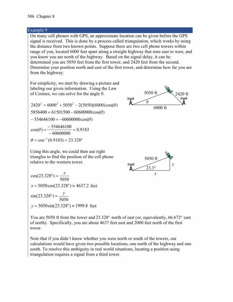
506 Chapter 8
Example 9 On many cell phones with GPS, an approximate location can be given before the GPS signal is received. This is done by a process called triangulation, which works by using the distance from two known points. Suppose there are two cell phone towers within range of you, located 6000 feet apart along a straight highway that runs east to west, and you know you are north of the highway. Based on the signal delay, it can be determined you are 5050 feet from the first tower, and 2420 feet from the second. Determine your position north and east of the first tower, and determine how far you are from the highway. For simplicity, we start by drawing a picture and labeling our given information. Using the Law of Cosines, we can solve for the angle θ.
)cos()6000)(5050(2505060002420 222 θ−+= )cos(60600000615015005856400 θ−=
)cos(60600000554646100 θ−=−
9183.060600000
554646100)cos( =−−
=θ
°== − 328.23)9183.0(cos 1θ Using this angle, we could then use right triangles to find the position of the cell phone relative to the western tower.
5050)328.23cos( x=°
2.4637)328.23cos(5050 š=x feet
5050)328.23sin( y=°
8.1999)328.23sin(5050 ≈°=y feet You are 5050 ft from the tower and °328.23 north of east (or, equivalently, 66.672° east of north). Specifically, you are about 4637 feet east and 2000 feet north of the first tower. Note that if you didn’t know whether you were north or south of the towers, our calculations would have given two possible locations, one north of the highway and one south. To resolve this ambiguity in real world situations, locating a position using triangulation requires a signal from a third tower.
2420 ft 5050 ft
6000 ft θ
5050 ft
23.3° y
x

Section 8.1 Non-Right Triangles: Laws of Sines and Cosines 507
Example 10 To measure the height of a hill, a woman measures the angle of elevation to the top of the hill to be 24 degrees. She then moves back 200 feet and measures the angle of elevation to be 22 degrees. Find the height of the hill. As with many problems of this nature, it will be helpful to draw a picture.
Notice there are three triangles formed here – the right triangle including the height h and the 22 degree angle, the right triangle including the height h and the 24 degree angle, and the (non-right) obtuse triangle including the 200 ft side. Since this is the triangle we have the most information for, we will begin with it. It may seem odd to work with this triangle since it does not include the desired side h, but we don’t have enough information to work with either of the right triangles yet. We can find the obtuse angle of the triangle, since it and the angle of 24 degrees complete a straight line – a 180 degree angle. The obtuse angle must be 180° - 24° = 156°. From this, we can determine that the third angle is 2°. We know one side is 200 feet, and its corresponding angle is 2°, so by introducing a temporary variable x for one of the other sides (as shown below), we can use Law of Sines to solve for this length x.
)2sin(200
)22sin( °=
°x Setting up the Law of Sines
)2sin(200)22sin(
°°=x isolating the x value
77.2146=x ft Now that we know x, we can use right triangle properties to solve for h.
77.2146hypotenuseopposite)24sin( h
xh===°
17.873)24sin(77.2146 =°=h ft. The hill is 873 feet high.
24° 22°
200 ft
h 156°
2°
x
24° 22° 200 ft
h

508 Chapter 8
Important Topics of This Section Law of Sines Solving for sides Solving for angles Ambiguous case, 0, 1 or 2 solutions Law of Cosines Solving for sides Solving for angles Generalized Pythagorean Theorem
Try it Now Answers
1. ( ) ( )121
sin120
80sin β=
°
1st possible solution2.358.162.83
=°=°=
cγβ
2nd solution 9.62.3
8.96
=°=°=
cγβ
If we were given a picture of the triangle it may be possible to eliminate one of these
2. ( ) ( )10
sin120
80sin β=
° . °= 65.5β or °= 35.174β ; only the first is reasonable.
°=°−°−°= 35.948065.5180γ ( ) ( )
c°
=° 35.94sin
12080sin
25.101,35.94,65.5 =°=°= cγβ 3. )25cos()20)(10(22010 222 °−+=a . a = 11.725
( ) ( )10
sin725.1125sin β
=° . °= 1.21β or °= 9.158β ;
only the first is reasonable since 25° + 158.9° would exceed 180°. °=°−°−°= 9.133251.21180γ
725.11,9.133,1.21 =°=°= aγβ

Section 8.1 Non-Right Triangles: Laws of Sines and Cosines 509
Section 8.1 Exercises Solve for the unknown sides and angles of the triangles shown.
1. 2.
3. 4.
5. 6.
7. 8.
Assume α is opposite side a, β is opposite side b, and γ is opposite side c. Solve each triangle for the unknown sides and angles if possible. If there is more than one possible solution, give both.
9. 20, 69, 43 =°=°= bγα 10. 19, 73, 35 =°=°= bγα
11. 14, 26, 119 ==°= baα 12. 32, 10, 113 ==°= cbγ
13. 45,105, 50 ==°= baβ 14. 38,49, 67 ==°= baβ
15. 8.242,2.184, 1.43 ==°= baα 16. 2.242,2.186, 6.36 ==°= baα
30
50 30° 18
40°
25
70° 90
100 65°
5 6
75°
45°
15
120° 6
25°
40° 110°
18
70° 50°
10

510 Chapter 8
Solve for the unknown sides and angles of the triangles shown.
17. 18.
19. 20.
Assume α is opposite side a, β is opposite side b, and γ is opposite side c. Solve each triangle for the unknown sides and angles if possible. If there is more than one possible solution, give both.
21. 13.3, 49.2, 2.41 ==°= baγ 22. 7.15, 6.10, 7.58 ==°= caβ
23. 7, 6, 120 ==°= cbα 24. 23,18, 115 ==°= baγ
25. Find the area of a triangle with sides of length 18, 21, and 32.
26. Find the area of a triangle with sides of length 20, 26, and 37.
27. To find the distance across a small lake, a surveyor has taken the measurements shown. Find the distance across the lake.
28. To find the distance between two cities, a satellite calculates the distances and angle shown (not to scale). Find the distance between the cities.
5
8
10 13
11
20
30° 16 10
60° 20 28
800 ft 900 ft 70°
350 km 370 km 2.1°

Section 8.1 Non-Right Triangles: Laws of Sines and Cosines 511
29. To determine how far a boat is from shore, two radar stations 500 feet apart determine the angles out to the boat, as shown. Find the distance of the boat from the station A, and the distance of the boat from shore.
30. The path of a satellite orbiting the earth causes it to pass directly over two tracking stations A and B, which are 69 mi apart. When the satellite is on one side of the two stations, the angles of elevation at A and B are measured to be 86.2° and 83.9°, respectively. How far is the satellite from station A and how high is the satellite above the ground?
31. A communications tower is located at the top of a steep hill, as shown. The angle of inclination of the hill is 67°. A guy-wire is to be attached to the top of the tower and to the ground, 165 m downhill from the base of the tower. The angle formed by the guy-wire and the hill is 16°. Find the length of the cable required for the guy wire.
32. The roof of a house is at a 20° angle. An 8 foot solar panel is to be mounted on the roof, and should be angled 38° relative to the horizontal for optimal results. How long does the vertical support holding up the back of the panel need to be?
33. A 127 foot tower is located on a hill that is inclined 38° to the horizontal. A guy-wire is to be attached to the top of the tower and anchored at a point 64 feet downhill from the base of the tower. Find the length of wire needed.
70° A
60° B
86.2° 83.9° A B
67°
16° 165m
38° 64 ft
127 ft
20° 38°
8 ft

512 Chapter 8
34. A 113 foot tower is located on a hill that is
inclined 34° to the horizontal. A guy-wire is to be attached to the top of the tower and anchored at a point 98 feet uphill from the base of the tower. Find the length of wire needed.
35. A pilot is flying over a straight highway. He determines the angles of depression to two mileposts, 6.6 km apart, to be 37° and 44°, as shown in the figure. Find the distance of the plane from point A, and the elevation of the plane.
36. A pilot is flying over a straight highway. He determines the angles of depression to two mileposts, 4.3 km apart, to be 32° and 56°, as shown in the figure. Find the distance of the plane from point A, and the elevation of the plane.
37. To estimate the height of a building, two students find the angle of elevation from a point (at ground level) down the street from the building to the top of the building is 39°. From a point that is 300 feet closer to the building, the angle of elevation (at ground level) to the top of the building is 50°. If we assume that the street is level, use this information to estimate the height of the building.
38. To estimate the height of a building, two students find the angle of elevation from a point (at ground level) down the street from the building to the top of the building is 35°. From a point that is 300 feet closer to the building, the angle of elevation (at ground level) to the top of the building is 53°. If we assume that the street is level, use this information to estimate the height of the building.
39. A pilot flies in a straight path for 1 hour 30 min. She then makes a course correction, heading 10 degrees to the right of her original course, and flies 2 hours in the new direction. If she maintains a constant speed of 680 miles per hour, how far is she from her starting position?
34° 98 ft
113 ft
A B
37° 44°
A B
32° 56°

Section 8.1 Non-Right Triangles: Laws of Sines and Cosines 513
40. Two planes leave the same airport at the same time. One flies at 20 degrees east of north at 500 miles per hour. The second flies at 30 east of south at 600 miles per hour. How far apart are the planes after 2 hours?
41. The four sequential sides of a quadrilateral have lengths 4.5 cm, 7.9 cm, 9.4 cm, and 12.9 cm. The angle between the two smallest sides is 117°. What is the area of this quadrilateral?
42. The four sequential sides of a quadrilateral have lengths 5.7 cm, 7.2 cm, 9.4 cm, and 12.8 cm. The angle between the two smallest sides is 106°. What is the area of this quadrilateral?
43. Three circles with radii 6, 7, and 8, all touch as shown. Find the shaded area bounded by the three circles.
44. A rectangle is inscribed in a circle of radius 10 cm as shown. Find the shaded area, inside the circle but outside the rectangle.
55°
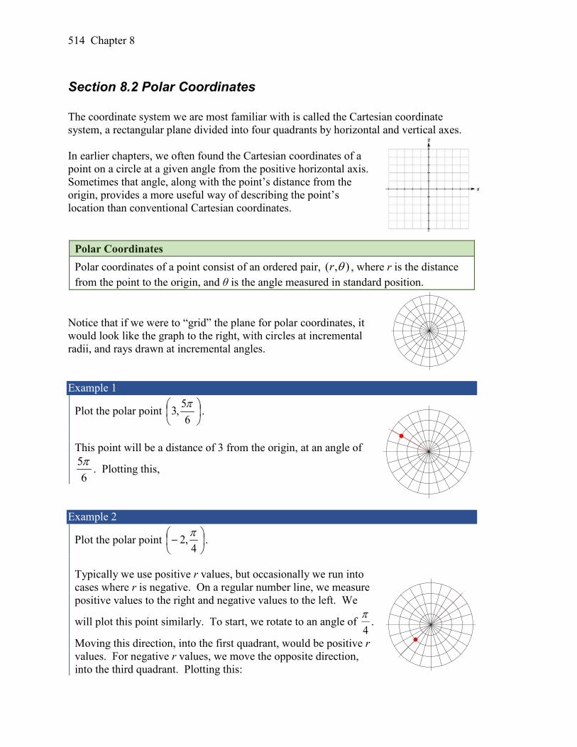
514 Chapter 8
Section 8.2 Polar Coordinates The coordinate system we are most familiar with is called the Cartesian coordinate system, a rectangular plane divided into four quadrants by horizontal and vertical axes. In earlier chapters, we often found the Cartesian coordinates of a point on a circle at a given angle from the positive horizontal axis. Sometimes that angle, along with the point’s distance from the origin, provides a more useful way of describing the point’s location than conventional Cartesian coordinates.
Polar Coordinates Polar coordinates of a point consist of an ordered pair, ),( θr , where r is the distance from the point to the origin, and θ is the angle measured in standard position.
Notice that if we were to “grid” the plane for polar coordinates, it would look like the graph to the right, with circles at incremental radii, and rays drawn at incremental angles. Example 1
Plot the polar point
65,3 π .
This point will be a distance of 3 from the origin, at an angle of
65π
. Plotting this,
Example 2
Plot the polar point
−
4,2 π .
Typically we use positive r values, but occasionally we run into cases where r is negative. On a regular number line, we measure positive values to the right and negative values to the left. We
will plot this point similarly. To start, we rotate to an angle of 4π
.
Moving this direction, into the first quadrant, would be positive r values. For negative r values, we move the opposite direction, into the third quadrant. Plotting this:

Section 8.2 Polar Coordinates 515
Note the resulting point is the same as the polar point 52,4π
. In fact, any Cartesian
point can be represented by an infinite number of different polar coordinates by adding or subtracting full rotations to these points. For example, same point could also be
represented as 132,4π
.
Try it Now 1. Plot the following points given in polar coordinates and label them.
a. 3,6
A π =
b. 2,3
B π = −
c. 34,4
C π =
Converting Points To convert between polar coordinates and Cartesian coordinates, we recall the relationships we developed back in Chapter 5.
Converting Between Polar and Cartesian Coordinates To convert between polar ),( θr and Cartesian (x, y) coordinates, we use the relationships
rx
=)cos(θ )cos(θrx =
ry
=)sin(θ )sin(θry =
xy
=)tan(θ 222 ryx =+
From these relationship and our knowledge of the unit circle, if r = 1 and 3πθ = , the
polar coordinates would be ( , ) 1,3
r πθ =
, and the corresponding Cartesian coordinates
1 3( , ) ,2 2
x y
=
.
(x, y)
r
θ y
x

516 Chapter 8
Remembering your unit circle values will come in very handy as you convert between Cartesian and polar coordinates. Example 3
Find the Cartesian coordinates of a point with polar coordinates
=
32,5),( πθr .
To find the x and y coordinates of the point,
25
215
32cos5)cos( −=
−=
==πθrx
235
235
32sin5)sin( =
=
==πθry
The Cartesian coordinates are
−
235,
25 .
Example 4
Find the polar coordinates of the point with Cartesian coordinates )4,3( −− . We begin by finding the distance r using the Pythagorean relationship 222 ryx =+
222 )4()3( r=−+− 29 16 r+ =
252 =r 5=r
Now that we know the radius, we can find the angle using any of the three trig relationships. Keep in mind that any of the relationships will produce two solutions on the circle, and we need to consider the quadrant to determine which solution to accept. Using the cosine, for example:
53)cos( −
==rxθ
214.253cos 1 ≈
−= −θ By symmetry, there is a second possibility at
069.4214.22 =−= πθ Since the point (-3, -4) is located in the 3rd quadrant, we can determine that the second angle is the one we need. The polar coordinates of this point are )069.4,5(),( =θr .
Try it Now

Section 8.2 Polar Coordinates 517
2. Convert the following. a. Convert polar coordinates ( )πθ ,2),( =r to ),( yx . b. Convert Cartesian coordinates )4,0(),( −=yx to ),( θr .
Polar Equations Just as a Cartesian equation like 2xy = describes a relationship between x and y values on a Cartesian grid, a polar equation can be written describing a relationship between r and θ values on the polar grid. Example 5
Sketch a graph of the polar equation θ=r . The equation θ=r describes all the points for which the radius r is equal to the angle. To visualize this relationship, we can create a table of values.
We can plot these points on the plane, and then sketch a curve that fits the points. The resulting graph is a spiral. Notice that the resulting graph cannot be the result of a function of the form y = f(x), as it does not pass the vertical line test, even though it resulted from a function giving r in terms of θ.
Although it is nice to see polar equations on polar grids, it is more common for polar graphs to be graphed on the Cartesian coordinate system, and so, the remainder of the polar equations will be graphed accordingly. The spiral graph above on a Cartesian grid is shown here. Example 6
Sketch a graph of the polar equation 3=r . Recall that when a variable does not show up in the equation, it is saying that it does not matter what value that variable has; the output for the equation will remain the same. For example, the Cartesian equation y = 3 describes all the points where y = 3, no matter what the x values are, producing a horizontal line.
θ 0 π/4 π/2 3π/4 π 5π/4 3π/2 7π/4 2π r 0 π/4 π/2 3π/4 π 5π/4 3π/2 7π/4 2π

518 Chapter 8
Likewise, this polar equation is describing all the points at a distance of 3 from the origin, no matter what the angle is, producing the graph of a circle.
The normal settings on graphing calculators and software graph on the Cartesian coordinate system with y being a function of x, where the graphing utility asks for f(x), or simply y =. To graph polar equations, you may need to change the mode of your calculator to Polar. You will know you have been successful in changing the mode if you now have r as a function of θ, where the graphing utility asks for r(θ), or simply r =. Example 7
Sketch a graph of the polar equation )cos(4 θ=r , and find an interval on which it completes one cycle. While we could again create a table, plot the corresponding points, and connect the dots, we can also turn to technology to directly graph it. Using technology, we produce the graph shown here, a circle passing through the origin. Since this graph appears to close a loop and repeat itself, we might ask what interval of θ values yields the entire graph. At θ = 0, 4)0cos(4 ==r , yielding the point (4, 0). We want the next θ value when the graph returns to the point (4, 0). Solving for when x = 4 is equivalent to solving 4)cos( =θr .
4)cos( =θr Substituting the equation for r gives 4)cos()cos(4 =θθ Dividing by 4 and simplifying
1)(cos2 =θ This has solutions when 1)cos( =θ or 1)cos( −=θ Solving these gives solutions
0=θ or πθ = This shows us at 0 radians we are at the point (0, 4), and again atπ radians we are at the point (0, 4) having finished one complete revolution. The interval πθ <≤0 yields one complete iteration of the circle.
Try it Now 3. Sketch a graph of the polar equation 3sin( )r θ= , and find an interval on which it
completes one cycle.

Section 8.2 Polar Coordinates 519
The last few examples have all been circles. Next, we will consider two other “named” polar equations, limaçons and roses. Example 8
Sketch a graph of the polar equation 2)sin(4 += θr . What interval of θ values corresponds to the inner loop? This type of graph is called a limaçon. Using technology, we can draw the graph. The inner loop begins and ends at the origin, where r = 0. We can solve for the θ values for which r = 0.
2)sin(40 += θ )sin(42 θ=−
21)sin( −=θ
67πθ = or
611πθ =
This tells us that r = 0, so the graph passes through the origin, twice on the interval [0, 2π).
The inner loop arises from the interval 6
116
7 πθπ≤≤ .
This corresponds to where the function 2)sin(4 += θr takes on negative values, as we could see if we graphed the function in the rθ plane.
Example 9
Sketch a graph of the polar equation )3cos( θ=r . What interval of θ values describes one small loop of the graph? This type of graph is called a 3 leaf rose. We can use technology to produce a graph. The interval [0, π) yields one cycle of this function. As with the last problem, we can note that there is an interval on which one loop of this graph begins and ends at the origin, where r = 0. Solving for θ,
)3cos(0 θ= Substitute u = 3θ )cos(0 u=
2π
=u or 2
3π=u or
25π
=u

520 Chapter 8
Undo the substitution,
23 πθ = or
233 πθ = or
253 πθ =
6πθ = or
2πθ = or
65πθ =
There are 3 solutions on πθ <≤0 which correspond to the 3 times the graph returns to the origin, but the first two solutions we solved for above are enough to conclude that
one loop corresponds to the interval 26πθπ
<≤ .
If we wanted to get an idea of how the computer drew this graph, consider when θ = 0.
cos(3 ) cos(0) 1r θ= = = , so the graph starts at (1,0). As we found above, at 6πθ = and
2πθ = , the graph is at the origin. Looking at the equation,
notice that any angle in between 6π
and 2π
, for example at
3πθ = , produces a negative r: ( )cos 3 cos 1
3r π π = ⋅ = = −
.
Notice that with a negative r value and an angle with terminal side in the first quadrant, the corresponding Cartesian point would be in the third quadrant. Since )3cos( θ=r is negative
on 26πθπ
<≤ , this interval corresponds to the loop of the graph in the third quadrant.
Try it Now 4. Sketch a graph of the polar equation sin(2 )r θ= . Would you call this function a
limaçon or a rose? Converting Equations While many polar equations cannot be expressed nicely in Cartesian form (and vice versa), it can be beneficial to convert between the two forms, when possible. To do this we use the same relationships we used to convert points between coordinate systems.
θ r x y 0 1 1 0
6π
0 0 0
3π
-1 12
− 32
−
2π
0 0 0

Section 8.2 Polar Coordinates 521
Example 10
Rewrite the Cartesian equation yyx 622 =+ as a polar equation. We wish to eliminate x and y from the equation and introduce r and θ. Ideally, we would like to write the equation with r isolated, if possible, which represents r as a function of θ.
yyx 622 =+ Remembering 222 ryx =+ we substitute
yr 62 = )sin(θry = and so we substitute again
)sin(62 θrr = Subtract )sin(6 θr from both sides
0)sin(62 =− θrr Factor ( ) 0)sin(6 =− θrr Use the zero factor theorem
)sin(6 θ=r or r = 0 Since r = 0 is only a point, we reject that solution. The solution )sin(6 θ=r is fairly similar to the one we graphed in Example 7. In fact, this equation describes a circle with bottom at the origin and top at the point (0, 6).
Example 11
Rewrite the Cartesian equation 23 += xy as a polar equation.
23 += xy Use )sin(θry = and )cos(θrx = 2)cos(3)sin( += θθ rr Move all terms with r to one side 2)cos(3)sin( =− θθ rr Factor out r
( ) 2)cos(3)sin( =− θθr Divide
)cos(3)sin(2
θθ −=r
In this case, the polar equation is more unwieldy than the Cartesian equation, but there are still times when this equation might be useful.
Example 12
Rewrite the polar equation )cos(21
3θ−
=r as a Cartesian equation.

522 Chapter 8
We want to eliminate θ and r and introduce x and y. It is usually easiest to start by clearing the fraction and looking to substitute values that will eliminate θ.
)cos(213
θ−=r Clear the fraction
( ) 3)cos(21 =− θr Use rx
=)cos(θ to eliminate θ
321 =
−
rxr Distribute and simplify
32 =− xr Isolate the r xr 23+= Square both sides
( )22 23 xr += Use 222 ryx =+ ( )222 23 xyx +=+
When our entire equation has been changed from r and θ to x and y we can stop unless asked to solve for y or simplify. In this example, if desired, the right side of the equation could be expanded and the equation simplified further. However, the equation cannot be written as a function in Cartesian form.
Try it Now 5. a. Rewrite the Cartesian equation in polar form: 23y x= ± − b. Rewrite the polar equation in Cartesian form: 2sin( )r θ=
Example 13
Rewrite the polar equation )2sin( θ=r in Cartesian form.
)2sin( θ=r Use the double angle identity for sine
)cos()sin(2 θθ=r Use rx
=)cos(θ and ry
=)sin(θ
ry
rxr ⋅⋅= 2 Simplify
2
2rxyr = Multiply by r2
xyr 23 = Since 222 ryx =+ , 22 yxr +=
( ) xyyx 23
22 =+

Section 8.2 Polar Coordinates 523
This equation could also be written as ( ) xyyx 22/322 =+ or ( ) 3/222 2xyyx =+
Important Topics of This Section Cartesian coordinate system Polar coordinate system Plotting points in polar coordinates Converting coordinates between systems Polar equations: Spirals, circles, limaçons and roses Converting equations between systems
Try it Now Answers
1. 2. a. ( )( , ) 2,r θ π= converts to ( )( , ) 2cos( ), 2sin( ) ( 2,0)x y π π= = −
b. ( )( , ) 0, 4x y = − converts to 3( , ) 4, 4,2 2
r orπ πθ = −
3. 3sin( ) 0θ = at 0=θ and πθ = .
It completes one cycle on the interval πθ <≤0 . 4. This is a 4-leaf rose. 5. a. 23y x= ± − can be rewritten as 2 2 3x y+ = , and becomes 3r =
A
B
C
524 Chapter 8
b. 2sin( )r θ= . 2 yrr
= . 2 2r y= . 2 2 2x y y+ =

Section 8.2 Polar Coordinates 525
Section 8.2 Exercises Convert the given polar coordinates to Cartesian coordinates.
1. 77,6π
2. 36,4π
3. 74,4π
4. 49,3π
5.
−
4, 6 π
6. 12,3π −
7. 3,
2π
8. ( )5,π
9. 3,6π −
10. 22,
3π −
11. (3, 2) 12. (7,1)
Convert the given Cartesian coordinates to polar coordinates. 13. (4, 2) 14. (8, 8) 15. ( 4, 6)− 16. ( 5,1 )−
17. (3, 5)− 18. (6, 5)− 19. ( )10, 13− − 20. ( 4, 7)− −
Convert the given Cartesian equation to a polar equation. 21. 3x = 22. 4y = 23. 24y x= 24. 42y x=
25. 2 2 4x y y+ = 26. 2 2 3x y x+ = 27. 2 2x y x− = 28. 2 2 3x y y− =
Convert the given polar equation to a Cartesian equation. 29. ( )3sinr θ= 30. ( )4cosr θ=
31. ( ) ( )
4sin 7cos
rθ θ
=+
32. ( ) ( )
6cos 3sin
rθ θ
=+
33. ( )2secr θ= 34. ( )3cscr θ=
35. ( )cos 2r r θ= + 36. ( ) ( )2 4sec cscr θ θ=

526 Chapter 8
Match each equation with one of the graphs shown. 37. ( )2 2cosr θ= + 38. ( )2 2sinr θ= + 39. ( )4 3cosr θ= +
40. ( )3 4cosr θ= + 41. 5r = 42. ( )2sinr θ=
A B C
D E F
Match each equation with one of the graphs shown.
43. ( )logr θ= 44. ( )cosr θ θ= 45. cos2
r θ =
46. ( ) ( )2sin cosr θ θ= 47. ( )1 2sin 3r θ= + 48. ( )1 sin 2r θ= +
A B C
D E F

Section 8.2 Polar Coordinates 527
Sketch a graph of the polar equation. 49. ( )3cosr θ= 50. ( )4sinr θ= 51. ( )3sin 2r θ=
52. ( )4sin 4r θ= 53. ( )5sin 3r θ= 54. ( )4sin 5r θ=
55. ( )3cos 2r θ= 56. ( )4cos 4r θ= 57. ( )2 2cosr θ= +
58. ( )3 3sinr θ= + 59. ( )1 3sinr θ= + 60. ( )2 4cosr θ= +
61. 2r θ= 62. 1rθ
=
63. ( )3 secr θ= + , a conchoid 64. θ1
=r , a lituus1
65. ( ) ( )2sin tanr θ θ= , a cissoid 66. ( )22 1 sinr θ= − , a hippopede
1 This curve was the inspiration for the artwork featured on the cover of this book.

528 Chapter 8
Section 8.3 Polar Form of Complex Numbers From previous classes, you may have encountered “imaginary numbers” – the square roots of negative numbers – and, more generally, complex numbers which are the sum of a real number and an imaginary number. While these are useful for expressing the solutions to quadratic equations, they have much richer applications in electrical engineering, signal analysis, and other fields. Most of these more advanced applications rely on properties that arise from looking at complex numbers from the perspective of polar coordinates. We will begin with a review of the definition of complex numbers.
Imaginary Number i
The most basic complex number is i, defined to be 1−=i , commonly called an imaginary number. Any real multiple of i is also an imaginary number.
Example 1
Simplify 9− . We can separate 9− as 19 − . We can take the square root of 9, and write the square root of -1 as i.
9− = i319 =− A complex number is the sum of a real number and an imaginary number.
Complex Number A complex number is a number biaz += , where a and b are real numbers a is the real part of the complex number b is the imaginary part of the complex number
1−=i Plotting a complex number We can plot real numbers on a number line. For example, if we wanted to show the number 3, we plot a point:

Section 8.3 Polar Form of Complex Numbers 529
To plot a complex number like i43− , we need more than just a number line since there are two components to the number. To plot this number, we need two number lines, crossed to form a complex plane.
Complex Plane In the complex plane, the horizontal axis is the real axis and the vertical axis is the imaginary axis.
Example 2
Plot the number i43− on the complex plane. The real part of this number is 3, and the imaginary part is -4. To plot this, we draw a point 3 units to the right of the origin in the horizontal direction and 4 units down in the vertical direction. Because this is analogous to the Cartesian coordinate system for plotting points, we can think about plotting our complex number biaz += as if we were plotting the point (a, b) in Cartesian coordinates. Sometimes people write complex numbers as z x yi= + to highlight this relation.
Arithmetic on Complex Numbers Before we dive into the more complicated uses of complex numbers, let’s make sure we remember the basic arithmetic involved. To add or subtract complex numbers, we simply add the like terms, combining the real parts and combining the imaginary parts. Example 3
Add i43− and i52 + . Adding )52()43( ii ++− , we add the real parts and the imaginary parts
ii 5423 +−+ i+5
Try it Now 1. Subtract i52 + from i43− .
real
imaginary

530 Chapter 8
We can also multiply and divide complex numbers. Example 4
Multiply: )52(4 i+ . To multiply the complex number by a real number, we simply distribute as we would when multiplying polynomials.
)52(4 i+ Distribute = i5424 ⋅+⋅ Simplify
i208 += Example 5
Multiply: )41)(32( ii +− . To multiply two complex numbers, we expand the product as we would with polynomials (the process commonly called FOIL – “first outer inner last”).
)41)(32( ii +− Expand
= 212382 iii −−+ Since 1−=i , 12 −=i = )1(12382 −−−+ ii Simplify = i514 +
Example 6
Divide (2 5 )(4 )
ii
+−
.
To divide two complex numbers, we have to devise a way to write this as a complex number with a real part and an imaginary part. We start this process by eliminating the complex number in the denominator. To do this, we multiply the numerator and denominator by a special complex number so that the result in the denominator is a real number. The number we need to multiply by is called the complex conjugate, in which the sign of the imaginary part is changed. Here, 4+i is the complex conjugate of 4–i. Of course, obeying our algebraic rules, we must multiply by 4+i on both the top and bottom. (2 5 ) (4 )(4 ) (4 )
i ii i
+ +⋅
− +
In the numerator,

Section 8.3 Polar Form of Complex Numbers 531
(2 5 )(4 )i i+ + Expand 28 20 2 5i i i= + + + Since 1−=i , 12 −=i
8 20 2 5( 1)i i= + + + − Simplify 3 22i= +
Multiplying the denominator (4 )(4 )i i− + Expand
2(16 4 4 )i i i− + − Since 1−=i , 12 −=i (16 ( 1))− − =17
Combining this we get 3 22 3 22
17 17 17i i+= +
Try it Now 2. Multiply i43− and 2 3i+ . With the interpretation of complex numbers as points in a plane, which can be related to the Cartesian coordinate system, you might be starting to guess our next step – to refer to this point not by its horizontal and vertical components, but using its polar location, given by the distance from the origin and an angle. Polar Form of Complex Numbers Remember, because the complex plane is analogous to the Cartesian plane that we can think of a complex number z x yi= + as analogous to the Cartesian point (x, y) and recall how we converted from (x, y) to polar (r, θ) coordinates in the last section. Bringing in all of our old rules we remember the following:
rx
=)cos(θ )cos(θrx =
ry
=)sin(θ )sin(θry =
xy
=)tan(θ 222 ryx =+
With this in mind, we can write cos( ) sin( )z x yi r irθ θ= + = + .
x + yi
r
θ y
x real
imaginary

532 Chapter 8
Example 7 Express the complex number i4 using polar coordinates. On the complex plane, the number 4i is a distance of 4 from
the origin at an angle of 2π
, so
+
=
2sin4
2cos44 ππ ii
Note that the real part of this complex number is 0.
In the 18th century, Leonhard Euler demonstrated a relationship between exponential and trigonometric functions that allows the use of complex numbers to greatly simplify some trigonometric calculations. While the proof is beyond the scope of this class, you will likely see it in a later calculus class.
Polar Form of a Complex Number and Euler’s Formula The polar form of a complex number is )sin()cos( θθ irrz += .
An alternate form, which will be the primary one used, is θirez = Euler’s Formula states )sin()cos( θθθ irrrei += Similar to plotting a point in the polar coordinate system we need r and θ to find the polar form of a complex number.
Example 8
Find the polar form of the complex number -8. Treating this is a complex number, we can write it as -8+0i. Plotted in the complex plane, the number -8 is on the negative horizontal axis, a distance of 8 from the origin at an angle of π from the positive horizontal axis. The polar form of the number -8 is πie8 . Plugging r = 8 and θ = π back into Euler’s formula, we have:
808)sin(8)cos(88 −=+−=+= iiei πππ as desired. Example 9

Section 8.3 Polar Form of Complex Numbers 533
Find the polar form of i44 +− . On the complex plane, this complex number would correspond to the point (-4, 4) on a Cartesian plane. We can find the distance r and angle θ as we did in the last section.
222 yxr += 222 4)4( +−=r
2432 ==r
To find θ, we can use rx
=)cos(θ
22
244)cos( −=
−=θ
This is one of known cosine values, and since the point is
in the second quadrant, we can conclude that 4
3πθ = .
The polar form of this complex number is i
e 43
24π
. Example 10
Find the polar form of i53 −− . On the complex plane, this complex number would correspond to the point (-3, -5) on a Cartesian plane. First, we find r.
222 yxr += 222 )5()3( −+−=r
34=r
To find θ, we might use xy
=)tan(θ
35)tan(
−−
=θ
0304.135tan 1 =
= −θ
This angle is in the wrong quadrant, so we need to find a second solution. For tangent, we can find that by adding π.
1720.40304.1 =+= πθ The polar form of this complex number is ie 1720.434 .
Try it Now

534 Chapter 8
3. Write 3 i+ in polar form.
Example 11
Write i
e 63π
in complex a bi+ form.
+
=
6sin3
6cos33 6 πππ
iei
Evaluate the trig functions
213
233 ⋅+⋅= i Simplify
23
233 i+=
The polar form of a complex number provides a powerful way to compute powers and roots of complex numbers by using exponent rules you learned in algebra. To compute a power of a complex number, we:
1) Convert to polar form 2) Raise to the power, using exponent rules to simplify 3) Convert back to a + bi form, if needed
Example 12
Evaluate ( )644 i+− . While we could multiply this number by itself five times, that would be very tedious. To compute this more efficiently, we can utilize the polar form of the complex number.
In an earlier example, we found that i
ei 43
2444π
=+− . Using this, ( )644 i+− Write the complex number in polar form
6
43
24
=
ie
π
Utilize the exponent rule mmm baab =)(
( )6
43
624
=
ie
π
On the second factor, use the rule mnnm aa =)(
( ) 64
36
24⋅
=i
eπ
Simplify i
e 29
32768π
= At this point, we have found the power as a complex number in polar form. If we want the answer in standard a + bi form, we can utilize Euler’s formula.
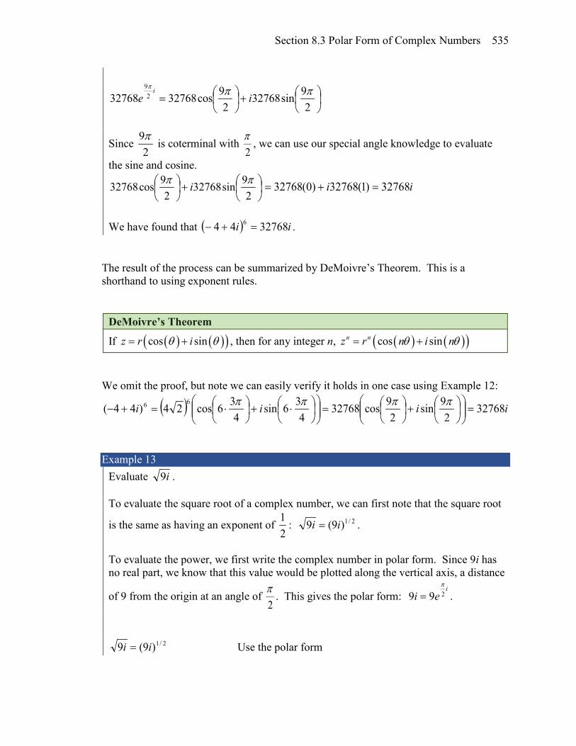
Section 8.3 Polar Form of Complex Numbers 535
+
=
29sin32768
29cos3276832768 2
9 πππ
iei
Since 2
9π is coterminal with
2π
, we can use our special angle knowledge to evaluate
the sine and cosine.
+
29sin32768
29cos32768 ππ i ii 32768)1(32768)0(32768 =+=
We have found that ( ) ii 3276844 6 =+− .
The result of the process can be summarized by DeMoivre’s Theorem. This is a shorthand to using exponent rules.
DeMoivre’s Theorem
If ( ) ( )( )cos sinz r iθ θ= + , then for any integer n, ( ) ( )( )cos sinn nz r n i nθ θ= + We omit the proof, but note we can easily verify it holds in one case using Example 12:
( ) iiii 327682
9sin2
9cos327684
36sin4
36cos24)44(66 =
+
=
⋅+
⋅=+−
ππππ
Example 13
Evaluate i9 . To evaluate the square root of a complex number, we can first note that the square root
is the same as having an exponent of 21
: 2/1)9(9 ii = .
To evaluate the power, we first write the complex number in polar form. Since 9i has no real part, we know that this value would be plotted along the vertical axis, a distance
of 9 from the origin at an angle of 2π
. This gives the polar form: i
ei 299π
= .
2/1)9(9 ii = Use the polar form

536 Chapter 8
=2/1
29
ieπ
Use exponent rules to simplify
2/1
22/19
=
ieπ
21
22/19⋅
=i
eπ
Simplify i
e 43π
= Rewrite using Euler’s formula if desired
+
=
4sin3
4cos3 ππ i Evaluate the sine and cosine
223
223 i+=
Using the polar form, we were able to find a square root of a complex number.
ii2
232
239 +=
Alternatively, using DeMoivre’s Theorem we could write
2/1
29
ieπ
= 1/2 1 19 cos sin 3 cos sin2 2 2 2 4 4
i iπ π π π ⋅ + ⋅ = + and simplify
Try it Now
4. Evaluate ( )63 i+ using polar form.
You may remember that equations like 42 =x have two solutions, 2 and -2 in this case, though the square root 4 only gives one of those solutions. Likewise, the square root we found in Example 11 is only one of two complex numbers whose square is 9i. Similarly, the equation 3 8z = would have three solutions where only one is given by the cube root. In this case, however, only one of those solutions, z = 2, is a real value. To find the others, we can use the fact that complex numbers have multiple representations in polar form. Example 14

Section 8.3 Polar Form of Complex Numbers 537
Find all complex solutions to 3 8z = . Since we are trying to solve 3 8z = , we can solve for z as 1/38z = . Certainly one of these solutions is the basic cube root, giving z = 2. To find others, we can turn to the polar representation of 8. Since 8 is a real number, is would sit in the complex plane on the horizontal axis at an angle of 0, giving the polar form ie08 . Taking the 1/3 power of this gives the real solution: ( ) ( ) 2)0sin(2)0cos(2288 03/103/13/10 =+=== ieee ii However, since the angle 2π is coterminal with the angle of 0, we could also represent the number 8 as ie π28 . Taking the 1/3 power of this gives a first complex solution:
( ) ( ) iiieeeiii 31
232
212
32sin2
32cos2288 3
23/123/13/12 +−=
+
−=
+
===
πππππ
For the third root, we use the angle of 4π, which is also coterminal with an angle of 0.
Altogether, we found all three complex solutions to 3 8z = , 2, 1 3 , 1 3z i i= − + − −
Graphed, these three numbers would be equally spaced on a circle about the origin at a radius of 2.
Important Topics of This Section Complex numbers Imaginary numbers Plotting points in the complex coordinate system Basic operations with complex numbers Euler’s Formula DeMoivre’s Theorem Finding complex solutions to equations

538 Chapter 8
Try it Now Answers 1. (3 4 ) (2 5 ) 1 9i i i− − + = −
2. (3 4 )(2 3 ) 18i i i− + = +
3. 3 i+ would correspond with the point ( )3,1 in the first quadrant.
2 23 1 4 2r = + = =
( ) 1sin2
θ = , so 6πθ =
3 i+ in polar form is 62i
eπ
4. ( )63 i+ = ( )6
662 2 64cos( ) 64sin( ) 64i ie e iπ π π π= = + = −

Section 8.3 Polar Form of Complex Numbers 539
Section 8.3 Exercises Simplify each expression to a single complex number. 1. 9− 2. 16− 3. 6 24− −
4. 3 75− − 5. 2 122
+ − 6. 4 202
+ −
Simplify each expression to a single complex number. 7. ( )3 2 (5 3 )i i+ + − 8. ( ) ( )2 4 1 6i i− − + +
9. ( )5 3 (6 )i i− + − − 10. ( )2 3 (3 2 )i i− − +
11. ( )2 3 (4 )i i+ 12. ( )5 2 (3 )i i−
13. ( )6 2 (5)i− 14. ( )( )2 4 8i− +
15. ( )2 3 (4 )i i+ − 16. ( )1 2 ( 2 3 )i i− + − +
17. ( )4 2 (4 2 )i i− + 18. ( )( )3 4 3 4i i+ −
19. 3 4
2i+
20. 6 2
3i−
21. 5 32
ii
− + 22.
6 4ii+
23. 2 34 3
ii
−+
24. 3 42
ii
+−
25. 6i 26. 11i 27. 17i 28. 24i
Rewrite each complex number from polar form into a bi+ form.
29. 23 ie 30. 44 ie 31. 66i
eπ
32. 38i
eπ
33. 543
ie
π
34. 745
ie
π
Rewrite each complex number into polar ire θ form. 35. 6 36. 8− 37. 4i− 38. 6i
39. 2 2i+ 40. 4 4i+ 41. 3 3i− + 42. 4 4i− −
43. 5 3i+ 44. 4 7i+ 45. 3 i− + 46. 2 3i− +
47. 1 4i− − 48. 3 6i− − 49. 5 i− 50. 1 3i−

540 Chapter 8
Compute each of the following, leaving the result in polar ire θ form.
51. 6 43 2 i i
e eπ π
52. 2 53 32 4
i ie e
π π
53.
34
6
6
3
i
i
e
e
π
π
54.
43
2
24
6
i
i
e
e
π
π 55. 10
42i
eπ
56. 4
63i
eπ
57. 2316
ie
π
58.329
ie
π
Compute each of the following, simplifying the result into a bi+ form. 59. ( )82 2i+ 60. ( )64 4i+ 61. 3 3i− +
62. 4 4i− − 63. 3 5 3i+ 64. 4 4 7i+
Solve each of the following equations for all complex solutions. 65. 5 2z = 66. 7 3z = 67. 6 1z = 68. 8 1z =

Section 8.4 Vectors 541
Section 8.4 Vectors A woman leaves home, walks 3 miles north, then 2 miles southeast. How far is she from home, and in which direction would she need to walk to return home? How far has she walked by the time she gets home? This question may seem familiar – indeed we did a similar problem with a boat in the first section of this chapter. In that section, we solved the problem using triangles. In this section, we will investigate another way to approach the problem using vectors, a geometric entity that indicates both a distance and a direction. We will begin our investigation using a purely geometric view of vectors. A Geometric View of Vectors
Vector A vector is an object that has both a length and a direction. Geometrically, a vector can be represented by an arrow that has a fixed length and indicates a direction. If, starting at the point A, a vector, which means “carrier” in
Latin, moves toward point B, we write AB to represent the vector. A vector may also be indicated using a single letter in boldface type, like u, or by capping the letter representing the vector with an arrow, like u .
Example 1
Draw a vector that represents the movement from the point P(-1, 2) to the point Q(3,3) By drawing an arrow from the first point to the second, we can construct a vector PQ .
Try it Now 1. Draw a vector, , that travels from the origin to the point (3, 5).
v

542 Chapter 8
Using this geometric representation of vectors, we can visualize the addition and scaling of vectors. To add vectors, we envision a sum of two movements. To find vu
+ , we first draw the vector u , then from the end of u we drawn the vector v . This corresponds to the notion that first we move along the first vector, and then from that end position we move along the second vector. The sum vu
+ is the new vector that travels directly from the beginning of u to the end of v in a straight path.
Adding Vectors Geometrically To add vectors geometrically, draw v starting from the end of
. The sum vu
+ is the vector from the beginning of to the end of v .
Example 2
Given the two vectors shown below, draw We draw v starting from the end of , then draw in the sum
vu
+ from the beginning of to the end of v .
Notice that path of the walking woman from the beginning of the section could be visualized as the sum of two vectors. The resulting sum vector would indicate her end position relative to home. Although vectors can exist anywhere in the plane, if we put the starting point at the origin it is easy to understand its size and direction relative to other vectors. To scale vectors by a constant, such as u3 , we can imagine adding uuu
++ . The result will be a vector three times as long in the same direction as the original vector. If we were to scale a vector by a negative number, such as u− , we can envision this as the opposite of u ; the vector so that )( uu
−+ returns us to the starting point. This vector u− would point in the opposite direction as u but have the same length.
u u
vu
+
u
u
u
v
vu
+
u v
u
v
vu
+

Section 8.4 Vectors 543
Another way to think about scaling a vector is to maintain its direction and multiply its length by a constant, so that u3 would point in the same direction but will be 3 times as long.
Scaling a Vector Geometrically To geometrically scale a vector by a constant, scale the length of the vector by the constant. Scaling a vector by a negative constant will reverse the direction of the vector.
Example 3
Given the vector shown, draw u3 , u− , and u2− . The vector u3 will be three times as long. The vector u− will have the same length but point in the opposite direction. The vector will point in the opposite direction and be twice as long.
By combining scaling and addition, we can find the difference between vectors geometrically as well, since )( vuvu
−+=− . Example 4
Given the vectors shown, draw From the end of u we draw , then draw in the result.
u2−
vu
−
v−
u
u3 u−
u2−
u v−
vu
−
u v

544 Chapter 8
Notice that the sum and difference of two vectors are the two diagonals of a parallelogram with the vectors u and as edges. Try it Now 2. Using vector v from Try it Now #1, draw . Component Form of Vectors While the geometric interpretation of vectors gives us an intuitive understanding of vectors, it does not provide us a convenient way to do calculations. For that, we need a handy way to represent vectors. Since a vector involves a length and direction, it would be logical to want to represent a vector using a length and an angle θ, usually measured from standard position.
Magnitude and Direction of a Vector
A vector u can be described by its magnitude, or length, u , and an angle θ.
A vector with length 1 is called unit vector. While this is very reasonable, and a common way to describe vectors, it is often more convenient for calculations to represent a vector by horizontal and vertical components.
Component Form of a Vector The component form of a vector represents the vector using two components.
yxu ,= indicates the vector represents a displacement of x units horizontally and y
units vertically.
Notice how we can see the magnitude of the vector as the length of the hypotenuse of a right triangle, or in polar form as the radius, r.
v
v2−
u
θ x
y
u v vu
−
u v
vu
+
u
θ

Section 8.4 Vectors 545
Alternate Notation for Vector Components
Sometimes you may see vectors written as the combination of unit vectors and j
, where i
points the right and j
points up. In other words, 0,1=i
and .
In this notation, the vector 4,3 −=u would be written as jiu
43 −= since both indicate a displacement of 3 units to the right, and 4 units down.
While it can be convenient to think of the vector yxu ,=
as an arrow from the origin to the point (x, y), be sure to remember that most vectors can be situated anywhere in the plane, and simply indicate a displacement (change in position) rather than a position. It is common to need to convert from a magnitude and angle to the component form of the vector and vice versa. Happily, this process is identical to converting from polar coordinates to Cartesian coordinates, or from the polar form of complex numbers to the a+bi form. Example 5
Find the component form of a vector with length 7 at an angle of 135 degrees. Using the conversion formulas )cos(θrx = and )sin(θry = , we can find the components
227)135cos(7 −=°=x
227)135sin(7 =°=y
This vector can be written in component form as 2
27,2
27− .
Example 6
Find the magnitude and angle θ representing the vector 2,3 −=u . First we can find the magnitude by remembering the relationship between x, y and r:
13)2(3 222 =−+=r 13=r
Second we can find the angle. Using the tangent,
i
1,0=j

546 Chapter 8
32)tan( −
=θ
°−≈
−= − 69.33
32tan 1θ , or written as a coterminal positive angle, 326.31°. This
angle is in the 4th quadrant as desired. Try it Now 3. Using vector v from Try it Now #1, the vector that travels from the origin to the point
(3, 5), find the components, magnitude and angle θ that represent this vector. In addition to representing distance movements, vectors are commonly used in physics and engineering to represent any quantity that has both direction and magnitude, including velocities and forces. Example 7
An object is launched with initial velocity 200 meters per second at an angle of 30 degrees. Find the initial horizontal and vertical velocities. By viewing the initial velocity as a vector, we can resolve the vector into horizontal and vertical components.
205.17323200)30cos(200 ≈⋅=°=x m/sec
10021200)30sin(200 =⋅=°=y m/sec
This tells us that, absent wind resistance, the object will travel horizontally at about 173 meters each second. Gravity will cause the vertical velocity to change over time – we’ll leave a discussion of that to physics or calculus classes.
Adding and Scaling Vectors in Component Form To add vectors in component form, we can simply add the corresponding components. To scale a vector by a constant, we scale each component by that constant.
200 m/s
30° 173 m/s
100 m/s

Section 8.4 Vectors 547
Combining Vectors in Component Form To add, subtract, or scale vectors in component form If 1 2,u u u= , 1 2,v v v=
, and c is any constant, then
2211 , vuvuvu ++=+
2211 , vuvuvu −−=−
21 ,cucuuc =
Example 8
Given 2,3 −=u and 4,1−=v , find a new vector vuw 23 −= Using the vectors given,
vuw 23 −= 4,122,33 −−−= Scale each vector
8,26,9 −−−= Subtract corresponding components
14,11 −= By representing vectors in component form, we can find the resulting displacement vector after a multitude of movements without needing to draw a lot of complicated non-right triangles. For a simple example, we revisit the problem from the opening of the section. The general procedure we will follow is:
1) Convert vectors to component form 2) Add the components of the vectors 3) Convert back to length and direction if needed to suit the context of the question
Example 9
A woman leaves home, walks 3 miles north, then 2 miles southeast. How far is she from home, and what direction would she need to walk to return home? How far has she walked by the time she gets home? Let’s begin by understanding the question in a little more depth. When we use vectors to describe a traveling direction, we often position things so north points in the upward direction, east points to the right, and so on, as pictured here. Consequently, travelling NW, SW, NE or SE, means we are travelling through the quadrant bordered by the given directions at a 45 degree angle. With this in mind, we begin by converting each vector to components.
N NE
E
SE S
SW
W
NW

548 Chapter 8
A walk 3 miles north would, in components, be 3,0 . A walk of 2 miles southeast would be at an angle of 45° South of East. Measuring from standard position the angle would be 315°. Converting to components, we choose to use the standard position angle so that we do not have to worry about whether the signs are negative or positive; they will work out automatically.
414.1,414.12
22,222)315sin(2),315cos(2 −≈
−⋅⋅=°°
Adding these vectors gives the sum of the movements in component form
586.1,414.1414.1,414.13,0 =−+ To find how far she is from home and the direction she would need to walk to return home, we could find the magnitude and angle of this vector.
Length = 125.2586.1414.1 22 =+ To find the angle, we can use the tangent
414.1586.1)tan( =θ
°=
= − 273.48
414.1586.1tan 1θ north of east
Of course, this is the angle from her starting point to her ending point. To return home, she would need to head the opposite direction, which we could either describe as 180°+48.273° = 228.273° measured in standard position, or as 48.273° south of west (or 41.727° west of south). She has walked a total distance of 3 + 2 + 2.125 = 7.125 miles. Keep in mind that total distance travelled is not the same as the length of the resulting displacement vector or the “return” vector.
Try it Now 4. In a scavenger hunt, directions are given to find a buried treasure. From a starting
point at a flag pole you must walk 30 feet east, turn 30 degrees to the north and travel 50 feet, and then turn due south and travel 75 feet. Sketch a picture of these vectors, find their components, and calculate how far and in what direction you must travel to go directly to the treasure from the flag pole without following the map.
3 2

Section 8.4 Vectors 549
While using vectors is not much faster than using law of cosines with only two movements, when combining three or more movements, forces, or other vector quantities, using vectors quickly becomes much more efficient than trying to use triangles. Example 10
Three forces are acting on an object as shown below, each measured in Newtons (N). What force must be exerted to keep the object in equilibrium (where the sum of the forces is zero)?
We start by resolving each vector into components. The first vector with magnitude 6 Newtons at an angle of 30 degrees will have components
3,33216,
236)30sin(6),30cos(6 =⋅⋅=°°
The second vector is only in the horizontal direction, so can be written as 0,7− . The third vector with magnitude 4 Newtons at an angle of 300 degrees will have components
32,22
34,214)300sin(4),300cos(4 −=
−⋅⋅=°°
To keep the object in equilibrium, we need to find a force vector yx, so the sum of
the four vectors is the zero vector, 0,0 .
3 3, 3 7, 0 2, 2 3 , 0, 0x y+ − + − + = Add component-wise
3 3 7 2, 3 0 2 3 , 0, 0x y− + + − + = Simplify
3 3 5, 3 2 3 , 0, 0x y− − + = Solve
, 0, 0 3 3 5, 3 2 3x y = − − −
, 3 3 5, 3 2 3 0.196, 0.464x y = − + − + ≈ −
30°
6 N 7 N
4 N 300°

550 Chapter 8
This vector gives in components the force that would need to be applied to keep the object in equilibrium. If desired, we could find the magnitude of this force and direction it would need to be applied in. Magnitude = 504.0464.0)196.0( 22 =+− N Angle:
196.0464.0)tan(
−=θ
°−=
−
= − 089.67196.0
464.0tan 1θ .
This is in the wrong quadrant, so we adjust by finding the next angle with the same tangent value by adding a full period of tangent:
°=°+°−= 911.112180089.67θ To keep the object in equilibrium, a force of 0.504 Newtons would need to be applied at an angle of 112.911°.
Important Topics of This Section Vectors, magnitude (length) & direction Addition of vectors Scaling of vectors Components of vectors Vectors as velocity Vectors as forces Adding & Scaling vectors in component form Total distance travelled vs. total displacement
Try it Now Answers
1 2.

Section 8.4 Vectors 551
2. °=
=== − 04.59
35tan34magnitude5,3 1θv
3.
50,301.7375)30sin(50),30cos(5030
75,0)30sin(50),30cos(500,30 321
−=−°°+=
−=°°==
fv
vvv
Magnitude = 88.73 feet at an angle of 34.3° south of east.
75 ft
50 ft 30 ft

552 Chapter 8
Section 8.4 Exercises Write the vector shown in component form.
1. 2. Given the vectors shown, sketch vu
+ , vu
− , and u2 .
3. 4. Write each vector below as a combination of the vectors u and v from question #3.
5. 6. From the given magnitude and direction in standard position, write the vector in component form. 7. Magnitude: 6, Direction: 45° 8. Magnitude: 10, Direction: 120° 9. Magnitude: 8, Direction: 220° 10. Magnitude: 7, Direction: 305° Find the magnitude and direction of the vector. 11. 4,0 12. 0,3− 13. 5,6 14. 7,3
15. 1,2− 16. 13,10− 17. 5,2 − 18. 4,8 −
19. 6,4 −− 20. 9,1− Using the vectors given, compute vu
+ , vu
− , and vu 32 − . 21. 5,1, 3,2 =−= vu 22. 1,2, 4,3 −=−= vu

Section 8.4 Vectors 553
23. A woman leaves home and walks 3 miles west, then 2 miles southwest. How far from home is she, and in what direction must she walk to head directly home?
24. A boat leaves the marina and sails 6 miles north, then 2 miles northeast. How far from the marina is the boat, and in what direction must it sail to head directly back to the marina?
25. A person starts walking from home and walks 4 miles east, 2 miles southeast, 5 miles south, 4 miles southwest, and 2 miles east. How far have they walked? If they walked straight home, how far would they have to walk?
26. A person starts walking from home and walks 4 miles east, 7 miles southeast, 6 miles south, 5 miles southwest, and 3 miles east. How far have they walked? If they walked straight home, how far would they have to walk?
27. Three forces act on an object: 7,4,1,0, 5,8 321 −==−−= FFF
. Find the net
force acting on the object.
28. Three forces act on an object: 7,0,3,8, 5,2 321 −=== FFF
. Find the net force
acting on the object.
29. A person starts walking from home and walks 3 miles at 20° north of west, then 5 miles at 10° west of south, then 4 miles at 15° north of east. If they walked straight home, how far would they have to walk, and in what direction?
30. A person starts walking from home and walks 6 miles at 40° north of east, then 2 miles at 15° east of south, then 5 miles at 30° south of west. If they walked straight home, how far would they have to walk, and in what direction?
31. An airplane is heading north at an airspeed of 600 km/hr, but there is a wind blowing from the southwest at 80 km/hr. How many degrees off course will the plane end up flying, and what is the plane’s speed relative to the ground?
32. An airplane is heading north at an airspeed of 500 km/hr, but there is a wind blowing from the northwest at 50 km/hr. How many degrees off course will the plane end up flying, and what is the plane’s speed relative to the ground?
33. An airplane needs to head due north, but there is a wind blowing from the southwest at 60 km/hr. The plane flies with an airspeed of 550 km/hr. To end up flying due north, the pilot will need to fly the plane how many degrees west of north?

554 Chapter 8
34. An airplane needs to head due north, but there is a wind blowing from the northwest
at 80 km/hr. The plane flies with an airspeed of 500 km/hr. To end up flying due north, the pilot will need to fly the plane how many degrees west of north?
35. As part of a video game, the point (5, 7) is rotated counterclockwise about the origin through an angle of 35 degrees. Find the new coordinates of this point.
36. As part of a video game, the point (7, 3) is rotated counterclockwise about the origin through an angle of 40 degrees. Find the new coordinates of this point.
37. Two children are throwing a ball back and forth straight across the back seat of a car. The ball is being thrown 10 mph relative to the car, and the car is travelling 25 mph down the road. If one child doesn't catch the ball and it flies out the window, in what direction does the ball fly (ignoring wind resistance)?
38. Two children are throwing a ball back and forth straight across the back seat of a car. The ball is being thrown 8 mph relative to the car, and the car is travelling 45 mph down the road. If one child doesn't catch the ball and it flies out the window, in what direction does the ball fly (ignoring wind resistance)?

Section 8.5 Dot Product 555
Section 8.5 Dot Product Now that we can add, subtract, and scale vectors, you might be wondering whether we can multiply vectors. It turns out there are two different ways to multiply vectors, one which results in a number, and one which results in a vector. In this section, we'll focus on the first, called the dot product or scalar product, since it produces a single numeric value (a scalar). We'll begin with some motivation. In physics, we often want to know how much of a force is acting in the direction of motion. To determine this, we need to know the angle between direction of force and the direction of motion. Likewise, in computer graphics, the lighting system determines how bright a triangle on the object should be based on the angle between object and the direction of the light. In both applications, we're interested in the angle between the vectors, so let's start there. Suppose we have two vectors, 21 , aaa =
and 21 ,bbb =
. Using our polar coordinate
conversions, we could write )sin(),cos( αα aaa
= and )sin(),cos( ββ bbb
= .
Now, if we knew the angles α and β, we wouldn't have much work to do - the angle between the vectors would be βαθ −= . While we certainly could use some inverse tangents to find the two angles, it would be great if we could find a way to determine the angle between the vector just from the vector components. To help us manipulate βαθ −= , we might try introducing a trigonometric function:
( ) ( )βαθ −= coscos Now we can apply the difference of angles identity
( ) ( ) ( ) ( ) ( )βαβαθ sinsincoscoscos +=
Now )cos(1 αaa
= , so aa
1)cos( =α , and likewise for the other three components.
Making those substitutions,
( )ba
bababb
aa
bb
aa
22112211cos+
=+=θ
( ) 2211cos bababa +=θ
Notice the expression on the right is a very simple calculation based on the components of the vectors. It comes up so frequently we define it to be the dot product of the two vectors, notated by a dot. This gives us two definitions of the dot product.
β
θ
α

556 Chapter 8
Definitions of the Dot Product
2211 bababa +=⋅
Component definition
( )θcosbaba
=⋅ Geometric definition
The first definition, 2211 bababa +=⋅
, gives us a simple way to calculate the dot product
from components. The second definition, ( )θcosbaba
=⋅ , gives us a geometric
interpretation of the dot product, and gives us a way to find the angle between two vectors, as we desired. Example 1
Find the dot product 1,52,3 ⋅− . Using the first definition, we can calculate the dot product by multiplying the x components and adding that to the product of the y components.
13215)1)(2()5)(3(1,52,3 =−=−+=⋅− Example 2
Find the dot product of the two vectors shown. We can immediately see that the magnitudes of the two vectors are 7 and 6. We can quickly calculate that the angle between the vectors is 150°. Using the geometric definition of the dot product,
( ) 3212342)150cos()7)(6(cos =⋅=°==⋅ θbaba
.
Try it Now 1. Calculate the dot product 6,23,7 −−⋅−
Now we can return to our goal of finding the angle between vectors.
30°
6 7

Section 8.5 Dot Product 557
Example 3 An object is being pulled up a ramp in the direction 1,5 by a
rope pulling in the direction 2,4 . What is the angle between the rope and the ramp? Using the component form, we can easily calculate the dot product.
22220)2)(1()4)(5(2,41,5 =+=+=⋅=⋅ba
We can also calculate the magnitude of each vector.
2615 22 =+=a , 2024 22 =+=b
Substituting these values into the geometric definition, we can solve for the angle between the vectors.
( )θcosbaba
=⋅
( )θcos202622 =
°≈
= − 255.15
202622cos 1θ .
Example 4
Calculate the angle between the vectors 4,6 and 3,2− . Calculating the dot product, 01212)3)(4()2)(6(3,24,6 =+−=+−=−⋅ We don't even need to calculate the magnitudes in this case since the dot product is 0.
( )θcosbaba
=⋅
( )θcos0 ba
=
( ) °==
= −− 900cos0cos 11
ba
θ
With the dot product equaling zero, as in the last example, the angle between the vectors will always be 90°, indicating that the vectors are orthogonal, a more general way of saying perpendicular. This gives us a quick way to check if vectors are orthogonal. Also, if the dot product is positive, then the inside of the inverse cosine will be positive, giving an angle less than 90°. A negative dot product will then lead to an angle larger than 90°

558 Chapter 8
Sign of the Dot Product If the dot product is: Zero The vectors are orthogonal (perpendicular). Positive The angle between the vectors is less than 90° Negative The angle between the vectors is greater than 90°
Try it Now 2. Are the vectors 3,7− and 6,2 −− orthogonal? If not, find the angle between them.
Projections In addition to finding the angle between vectors, sometimes we want to know how much one vector points in the direction of another. For example, when pulling an object up a ramp, we might want to know how much of the force is exerted in the direction of motion. To determine this we can use the idea of a projection.
In the picture above, u is a projection of a onto b
. In other words, it is the portion of a that points in the same direction as b
. To find the length of u , we could notice that it is one side of a right triangle. If we
define θ to be the angle between a and u , then au
=)cos(θ , so ua
=)cos(θ .
While we could find the angle between the vectors to determine this magnitude, we could skip some steps by using the dot product directly. Since )cos(θbaba
=⋅ ,
bbaa
⋅=)cos(θ . Using this, we can rewrite )cos(θau
= as b
bau
⋅= . This gives us
the length of the projection, sometimes denoted as b
bauacompb
⋅== .
a a
b
b
u
v

Section 8.5 Dot Product 559
To find the vector u itself, we could first scale b
to a unit vector with length 1: bb
.
Multiplying this by the length of the projection will give a vector in the direction of b
but with the correct length.
bb
babb
bba
bbuaprojb
⋅
=
⋅== 2
Projection Vector
The projection of vector a onto b
is bb
baaprojb
⋅
= 2
The magnitude of the projection is b
baacompb
⋅=
Example 5
Find the projection of the vector 2,3 − onto the vector 6,8 . We will need to know the dot product of the vectors and the magnitude of the vector we are projecting onto.
121224)6)(2()8)(3(6,82,3 =−=−+=⋅−
101003664686,8 22 ==+=+=
The magnitude of the projection will be 56
1012
6,86,82,3
==⋅−
.
To find the projection vector itself, we would multiply that magnitude by 6,8 scaled to a unit vector.
2518,
2524
5036,
50486,8
506
106,8
56
6,86,8
56
==== .
Based on the sketch above, this answer seems reasonable.

560 Chapter 8
Try it Now 3. Find the component of the vector 4,3− that is orthogonal to the vector 4,8−
Work In physics, when a constant force causes an object to move, the mechanical work done by that force is the product of the force and the distance the object is moved. However, we only consider the portion of force that is acting in the direction of motion. This is simply the magnitude of the projection of the force
vector onto the distance vector, d
dF
⋅ . The work done is the
product of that component of force times the distance moved, the magnitude of the distance vector.
dFdd
dFWork
⋅=
⋅=
It turns out that work is simply the dot product of the force vector and the distance vector.
Work
When a force F
causes an object to move some distance d
, the work done is
dFWork
⋅= Example 6
A cart is pulled 20 feet by applying a force of 30 pounds on a rope held at a 30 degree angle. How much work is done? Since work is simply the dot product, we can take advantage of the geometric definition of the dot product in this case.
615.519)30cos()20)(30()cos( ≈°=⋅=⋅= θdFdFWork
ft-lbs.
Try it Now 4. Find the work down moving an object from the point (1, 5) to (9, 14) by the force
vector 2,3=F
30°
30 pounds
20 feet
F
d
u

Section 8.5 Dot Product 561
Important Topics of This Section Calculate Dot Product Using component definition Using geometric definition Find the angle between two vectors Sign of the dot product Projections Work
Try it Now Answers 1. 41814)6)(3()2)(7(6,23,7 −=−=−+−−=−−⋅− 2. In the previous Try it Now, we found the dot product was -4, so the vectors are not
orthogonal. The magnitudes of the vectors are ( ) 5837 22 =+− and
( ) 4062 22 =+− . The angle between the vectors will be
°≈
−= − 764.94
40584cos 1θ
3. We want to find the component of 4,3− that is orthogonal to the
vector 4,8− . In the picture to the right, that component is vector v . Notice that avu
=+ , so if we can find the projection vector, we can find v .
( ) 2,44,880404,8
4)8(
4,84,32
222 −=−=−
+−
−⋅−=
⋅
== bb
baaproju b
.
Now we can solve avu
=+ for v . 2,12,44,3 =−−−=−= uav
4. The distance vector is 9,8514,19 =−− .
The work is the dot product: 4218249,82,3 =+=⋅=⋅= dFWork
a
b
u
v

562 Chapter 8
Section 8.5 Exercises Two vectors are described by their magnitude and direction in standard position. Find the dot product of the vectors. 1. Magnitude: 6, Direction: 45°; Magnitude: 10, Direction: 120° 2. Magnitude: 8, Direction: 220°; Magnitude: 7, Direction: 305° Find the dot product of each pair of vectors. 3. 4,0 ; 0,3− 4. 5,6 ; 7,3
5. 1,2− ; 13,10− 6. 5,2 − ; 4,8 − Find the angle between the vectors 7. 4,0 ; 0,3− 8. 5,6 ; 7,3
9. 4,2 ; 3,1 − 10. 1,4− ; 2,8 −
11. 2,4 ; 4,8 12. 3,5 ; 10,6− 13. Find a value for k so that 7,2 and 4,k will be orthogonal.
14. Find a value for k so that 5,3− and k,2 will be orthogonal. 15. Find the magnitude of the projection of 4,8 − onto 3,1 − .
16. Find the magnitude of the projection of 7,2 onto 5,4 .
17. Find the projection of 10,6− onto 3,1 − .
18. Find the projection of 4,0 onto 7,3 . 19. A scientist needs to determine the angle of reflection when a laser hits a mirror. The
picture shows the vector representing the laser beam, and a vector that is orthogonal to the mirror. Find the acute angle between these, the angle of reflection.
20. A triangle has coordinates at A: (1,4), B: (2,7), and C: (4,2). Find the angle at point B. 21. A boat is trapped behind a log lying parallel to the
dock. It only requires 10 pounds of force to pull the boat directly towards you, but because of the log, you'll have to pull at a 45° angle. How much force will you have to pull with? (We're going to assume that the log is very slimy and doesn't contribute any additional resistance.)

Section 8.5 Dot Product 563
22. A large boulder needs to be dragged to a new position. If pulled directly horizontally, the boulder would require 400 pounds of pulling force to move. We need to pull the boulder using a rope tied to the back of a large truck, forming a 15° angle from the ground. How much force will the truck need to pull with?
23. Find the work done against gravity by pushing a 20 pound cart 10 feet up a ramp that
is 10° above horizontal. Assume there is no friction, so the only force is 20 pounds downwards due to gravity.
24. Find the work done against gravity by pushing a 30 pound cart 15 feet up a ramp that
is 8° above horizontal. Assume there is no friction, so the only force is 30 pounds downwards due to gravity.
25. An object is pulled to the top of a 40 foot ramp that forms a 10°
angle with the ground. It is pulled by rope exerting a force of 120 pounds at a 35° angle relative to the ground. Find the work done.
26. An object is pulled to the top of a 30 foot ramp that forms a 20° angle with the
ground. It is pulled by rope exerting a force of 80 pounds at a 30° angle relative to the ground. Find the work done.
15°
10°
35°

564 Chapter 8
Section 8.6 Parametric Equations Many shapes, even ones as simple as circles, cannot be represented as an equation where y is a function of x. Consider, for example, the path a moon follows as it orbits around a planet, which simultaneously rotates around a sun. In some cases, polar equations provide a way to represent such a path. In others, we need a more versatile approach that allows us to represent both the x and y coordinates in terms of a third variable, or parameter.
Parametric Equations A system of parametric equations is a pair of functions x(t) and y(t) in which the x and y coordinates are the output, represented in terms of a third input parameter, t.
Example 1
Moving at a constant speed, an object moves at a steady rate along a straight path from coordinates (-5, 3) to the coordinates (3, -1) in 4 seconds, where the coordinates are measured in meters. Find parametric equations for the position of the object. The x coordinate of the object starts at -5 meters, and goes to +3 meters, this means the x direction has changed by 8 meters in 4 seconds, giving us a rate of 2 meters per second. We can now write the x coordinate as a linear function with respect to time, t,
ttx 25)( +−= . Similarly, the y value starts at 3 and goes to -1, giving a change in y value of 4 meters, meaning the y values have decreased by 4 meters in 4 seconds, for a rate of -1 meter per second, giving equation tty −= 3)( . Together, these are the parametric equations for the position of the object:
ttyttx
−=+−=
3)(25)(
Using these equations, we can build a table of t, x, and y values. Because of the context, we limited ourselves to non-negative t values for this example, but in general you can use any values. From this table, we could create three possible graphs: a graph of x vs. t, which would show the horizontal position over time, a graph of y vs. t, which would show the vertical position over time, or a graph of y vs. x, showing the position of the object in the plane.
t x y 0 -5 3 1 -3 2 2 -1 1 3 1 0 4 3 -1

Section 8.6 Parametric Equations 565
Position of x as a function of time Position of y as a function of time
Position of y relative to x
Notice that the parameter t does not explicitly show up in this third graph. Sometimes, when the parameter t does represent a quantity like time, we might indicate the direction of movement on the graph using an arrow, as shown above.
There is often no single parametric representation for a curve. In Example 1 we assumed the object was moving at a steady rate along a straight line. If we kept the assumption about the path (straight line) but did not assume the speed was constant, we might get a system like:
2
2
3)(25)(
ttyttx
−=
+−=
This starts at (-5, 3) when t = 0 and ends up at (3, -1) when t = 2. If we graph the x(t) and y(t) function separately, we can see that those are no longer linear, but if we graph x vs. y we will see that we still get a straight-line path.
t

566 Chapter 8
Example 2 Sketch a graph of
ttyttx+=+=
2)(1)( 2
We can begin by creating a table of values. From this table, we can plot the (x, y) points in the plane, sketch in a rough graph of the curve, and indicate the direction of motion with respect to time by using arrows.
Notice that here the parametric equations describe a shape for which y is not a function of x. This is an example of why using parametric equations can be useful – since they can represent such a graph as a set of functions. This particular graph also appears to be a parabola where x is a function of y, which we will soon verify. Example 3
Sketch a graph of ( ) 3cos( )( ) 3sin( )
x t ty t t
==
These equations should look familiar. Back when we first learned about sine and cosine we found that the coordinates of a point on a circle of radius r at an angle of θ will be
cos( ), sin( )x r y rθ θ= = . The equations above are in the same form, with 3r = , and t used in place of θ. This suggests that for each value of t, these parametric equations give a point on a circle of radius 3 at the angle corresponding to t. At 0t = , the graph would be at
3cos(0), 3sin(0)x y= = , the point (3,0). Indeed, these equations describe the equation of a circle, drawn counterclockwise.
t x y -3 10 -1 -2 5 0 -1 2 1 0 1 2 1 2 3 2 5 4
(rcos(θ), rsin(θ))
r
θ y
x
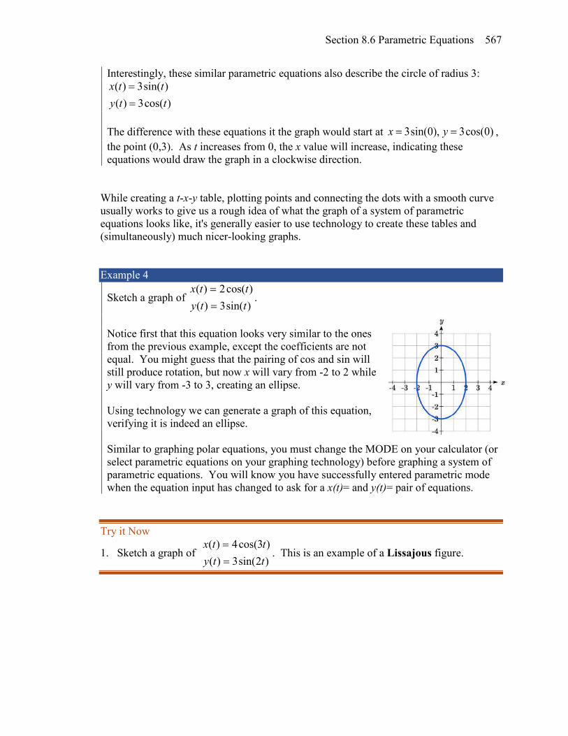
Section 8.6 Parametric Equations 567
Interestingly, these similar parametric equations also describe the circle of radius 3: ( ) 3sin( )( ) 3cos( )
x t ty t t
==
The difference with these equations it the graph would start at 3sin(0), 3cos(0)x y= = , the point (0,3). As t increases from 0, the x value will increase, indicating these equations would draw the graph in a clockwise direction.
While creating a t-x-y table, plotting points and connecting the dots with a smooth curve usually works to give us a rough idea of what the graph of a system of parametric equations looks like, it's generally easier to use technology to create these tables and (simultaneously) much nicer-looking graphs. Example 4
Sketch a graph of )sin(3)()cos(2)(
ttyttx
==
.
Notice first that this equation looks very similar to the ones from the previous example, except the coefficients are not equal. You might guess that the pairing of cos and sin will still produce rotation, but now x will vary from -2 to 2 while y will vary from -3 to 3, creating an ellipse. Using technology we can generate a graph of this equation, verifying it is indeed an ellipse. Similar to graphing polar equations, you must change the MODE on your calculator (or select parametric equations on your graphing technology) before graphing a system of parametric equations. You will know you have successfully entered parametric mode when the equation input has changed to ask for a x(t)= and y(t)= pair of equations.
Try it Now
1. Sketch a graph of )2sin(3)()3cos(4)(
ttyttx
==
. This is an example of a Lissajous figure.

568 Chapter 8
Example 5 The populations of rabbits and wolves on an island over time are given by the graphs below. Use these graphs to sketch a graph in the r-w plane showing the relationship between the number of rabbits and number of wolves.
For each input t, we can determine the number of rabbits, r, and the number of wolves, w, from the respective graphs, and then plot the corresponding point in the r-w plane.
This graph helps reveal the cyclical interaction between the two populations.
Converting from Parametric to Cartesian In some cases, it is possible to eliminate the parameter t, allowing you to write a pair of parametric equations as a Cartesian equation. It is easiest to do this if one of the x(t) or y(t) functions can easily be solved for t, allowing you to then substitute the remaining expression into the second part. Example 6
Write tty
ttx+=+=
2)(1)( 2
as a Cartesian equation, if possible.
Here, the equation for y is linear, so is relatively easy to solve for t. Since the resulting Cartesian equation will likely not be a function, and for convenience, we drop the function notation.
02468
1012141618
0 1 2 3 4 5 6 7
Wol
ves
Years
0
20
40
60
80
100
0 5 10 15 20
Rab
bits
Wolves
0
20
40
60
80
100
0 1 2 3 4 5 6 7
Rab
bits
Years

Section 8.6 Parametric Equations 569
ty += 2 Solve for t ty =− 2 Substitute this for t in the x equation
1)2( 2 +−= yx Notice that this is the equation of a parabola with x as a function of y, with vertex at (1,2), opening to the right. Comparing this with the graph from Example 2, we see (unsurprisingly) that it yields the same graph in the x-y plane as did the original parametric equations.
Try it Now
2. Write 6
3
)()(
ttyttx
=
=as a Cartesian equation, if possible.
Example 7
Write )log()(2)(
ttyttx
=+= as a Cartesian equation, if possible.
We could solve either the first or second equation for t. Solving the first,
2+= tx
tx =− 2 Square both sides
( ) tx =− 22 Substitute into the y equation
( )( )22log −= xy Since the parametric equation is only defined for 0>t , this Cartesian equation is equivalent to the parametric equation on the corresponding domain. The parametric equations show that when t > 0, x > 2 and y > 0, so the domain of the Cartesian equation should be limited to x > 2.
To ensure that the Cartesian equation is as equivalent as possible to the original parametric equation, we try to avoid using domain-restricted inverse functions, such as the inverse trig functions, when possible. For equations involving trig functions, we often try to find an identity to utilize to avoid the inverse functions.

570 Chapter 8
Example 8
Write )sin(3)()cos(2)(
ttyttx
==
as a Cartesian equation, if possible.
To rewrite this, we can utilize the Pythagorean identity 1)(sin)(cos 22 =+ tt .
)cos(2 tx = so )cos(2
tx=
)sin(3 ty = so )sin(3
ty=
Starting with the Pythagorean Identity,
1)(sin)(cos 22 =+ tt Substitute in the expressions from the parametric form
132
22
=
+
yx Simplify
194
22
=+yx
This is a Cartesian equation for the ellipse we graphed earlier.
Parameterizing Curves While converting from parametric form to Cartesian can be useful, it is often more useful to parameterize a Cartesian equation – converting it into parametric form. If the Cartesian equation gives one variable as a function of the other, then parameterization is trivial – the independent variable in the function can simply be defined as t. Example 9
Parameterize the equation yyx 23 −= . In this equation, x is expressed as a function of y. By defining ty = we can then substitute that into the Cartesian equation, yielding ttx 23 −= . Together, this produces the parametric form:
ttytttx
=−=
)(2)( 3

Section 8.6 Parametric Equations 571
Try it Now 3. Write 322 =+ yx in parametric form, if possible.
In addition to parameterizing Cartesian equations, we also can parameterize behaviors and movements. Example 10
A robot follows the path shown. Create a table of values for the x(t) and y(t) functions, assuming the robot takes one second to make each movement. Since we know the direction of motion, we can introduce consecutive values for t along the path of the robot. Using these values with the x and y coordinates of the robot, we can create the tables. For example, we designate the starting point, at (1, 1), as the position at t = 0, the next point at (3, 1) as the position at t = 1, and so on. Notice how this also ties back to vectors. The journey of the robot as it moves through the Cartesian plane could also be displayed as vectors and total distance traveled and displacement could be calculated.
Example 11
A light is placed on the edge of a bicycle tire as shown and the bicycle starts rolling down the street. Find a parametric equation for the position of the light after the wheel has rotated through an angle of θ.
Relative to the center of the wheel, the position of the light can be found as the coordinates of a point on a circle, but since the x coordinate begins at 0 and moves in the negative direction, while the y coordinate starts at the lowest value, the coordinates of the point will be given by:
θ
Starting Rotated by θ
r
t 0 1 2 3 4 5 6 x 1 3 3 2 4 1 1
t 0 1 2 3 4 5 6 y 1 1 2 2 4 5 4

572 Chapter 8
)cos()sin(θθ
ryrx−=−=
The center of the wheel, meanwhile, is moving horizontally. It remains at a constant height of r, but the horizontal position will move a distance equivalent to the arclength of the circle drawn out by the angle, θrs = . The position of the center of the circle is then
ryrx
== θ
Combining the position of the center of the wheel with the position of the light on the wheel relative to the center, we get the following parametric equationw, with θ as the parameter:
( )( ))cos(1)cos(
)sin()sin(θθθθθθ
−=−=−=−=
rrryrrrx
The result graph is called a cycloid.
Example 12
A moon travels around a planet as shown, orbiting once every 10 days. The planet travels around a sun as shown, orbiting once every 100 days. Find a parametric equation for the position of the moon, relative to the center of the sun, after t days. For this example, we’ll assume the orbits are circular, though in real life they’re actually elliptical.
6 30

Section 8.6 Parametric Equations 573
The coordinates of a point on a circle can always be written in the form
)sin()cos(
θθ
ryrx
==
Since the orbit of the moon around the planet has a period of 10 days, the equation for the position of the moon relative to the planet will be
=
=
=
=
ttty
tttx
5sin6
102sin6)(
5cos6
102cos6)(
ππ
ππ
With a period of 100 days, the equation for the position of the planet relative to the sun will be
=
=
=
=
ttty
tttx
50sin30
1002sin30)(
50cos30
1002cos30)(
ππ
ππ
Combining these together, we can find the position of the moon relative to the sun as the sum of the components.
+
=
+
=
ttty
tttx
50sin30
5sin6)(
50cos30
5cos6)(
ππ
ππ
The resulting graph is shown here.
Try it Now 4. A wheel of radius 4 is rolled around the outside of a circle of radius 7. Find a
parametric equation for the position of a point on the boundary of the smaller wheel. This shape is called an epicycloid.

574 Chapter 8
Important Topics of This Section Parametric equations Graphing x(t) , y(t) and the corresponding x-y graph Sketching graphs and building a table of values Converting parametric to Cartesian Converting Cartesian to parametric (parameterizing curves)
Try it Now Answers
1.
2. ( )23ty = , so 2xy =
3. )sin(3)()cos(3)(
ttyttx
==
4. The center of the small wheel rotates in circle with radius 7+4=11.
Since the circumference of the small circle is π8 and the circumference of the large circle is π22 , in the time it takes to roll around the large circle, the small circle will
have rotated 4
11822
=ππ
rotations. We use this as the stretch factor. The position of a
point on the small circle will be the combination of the position of the center of the small wheel around the center of the large wheel, and the position of the point around the small wheel:
( )
( )
11( ) 11cos 4cos4
11( ) 11sin 4sin4
x t t t
y t t t
= − = −

Section 8.6 Parametric Equations 575
Section 8.6 Exercises Match each set of equations with one of the graphs below.
1. ( )( ) 2 1
x t ty t t
= = −
2. ( )( ) 2
1x t ty t t
= − =
3. ( ) ( )( ) ( )
4sin2cos
x t ty t t
= =
4. ( )( )
2sin( )4cos( )
x t ty t t
= =
5. ( )( )
23 2
x t ty t t
= + = −
6. ( )( )
2 23
x t ty t t
= − − = +
A B C
D E F From each pair of graphs in the t-x and t-y planes shown, sketch a graph in the x-y plane.
7. 8.

576 Chapter 8
From each graph in the x-y plane shown, sketch a graph of the parameter functions in the t-x and t-y planes.
9. 10. Sketch the parametric equations for 2 2t− ≤ ≤ .
11. ( )( ) 2
1 2x t ty t t
= + =
12. ( )( ) 3
2 2x t ty t t
= − =
Eliminate the parameter t to rewrite the parametric equation as a Cartesian equation
13. ( )( )
58 2
x t ty t t
= − = −
14. ( )( )
6 310
x t ty t t
= − = −
15. ( )( )
2 1
3
x t t
y t t
= +
= 16. ( )
( ) 2
3 12
x t ty t t
= − =
17. ( )( )
21 5
tx t ey t t
= = −
18. ( ) ( )( )
4log3 2
x t ty t t
= = +
19. ( )( )
3
2x t t ty t t
= − =
20. ( )( )
4
2x t t ty t t
= − = +
21. ( )( )
2
6
t
t
x t ey t e
= =
22. ( )( )
5
10
x t ty t t
= =
23. ( ) ( )( ) ( )
4cos5sin
x t ty t t
= =
24. ( ) ( )( ) ( )
3sin6cos
x t ty t t
= =

Section 8.6 Parametric Equations 577
Parameterize (write a parametric equation for) each Cartesian equation 25. ( ) 23 3y x x= + 26. ( ) ( )2sin 1y x x= +
27. ( ) ( )3logx y y y= + 28. ( ) 2x y y y= +
29. 2 2
14 9x y
+ = 30. 2 2
116 36x y
+ =
Parameterize the graphs shown.
31. 32.
33. 34. 35. Parameterize the line from ( 1,5)− to (2,3) so that the line is at ( 1,5)− at t = 0, and at
(2, 3) at t = 1.
36. Parameterize the line from (4,1) to (6, 2)− so that the line is at (4,1) at t = 0, and at (6, 2)− at t = 1.
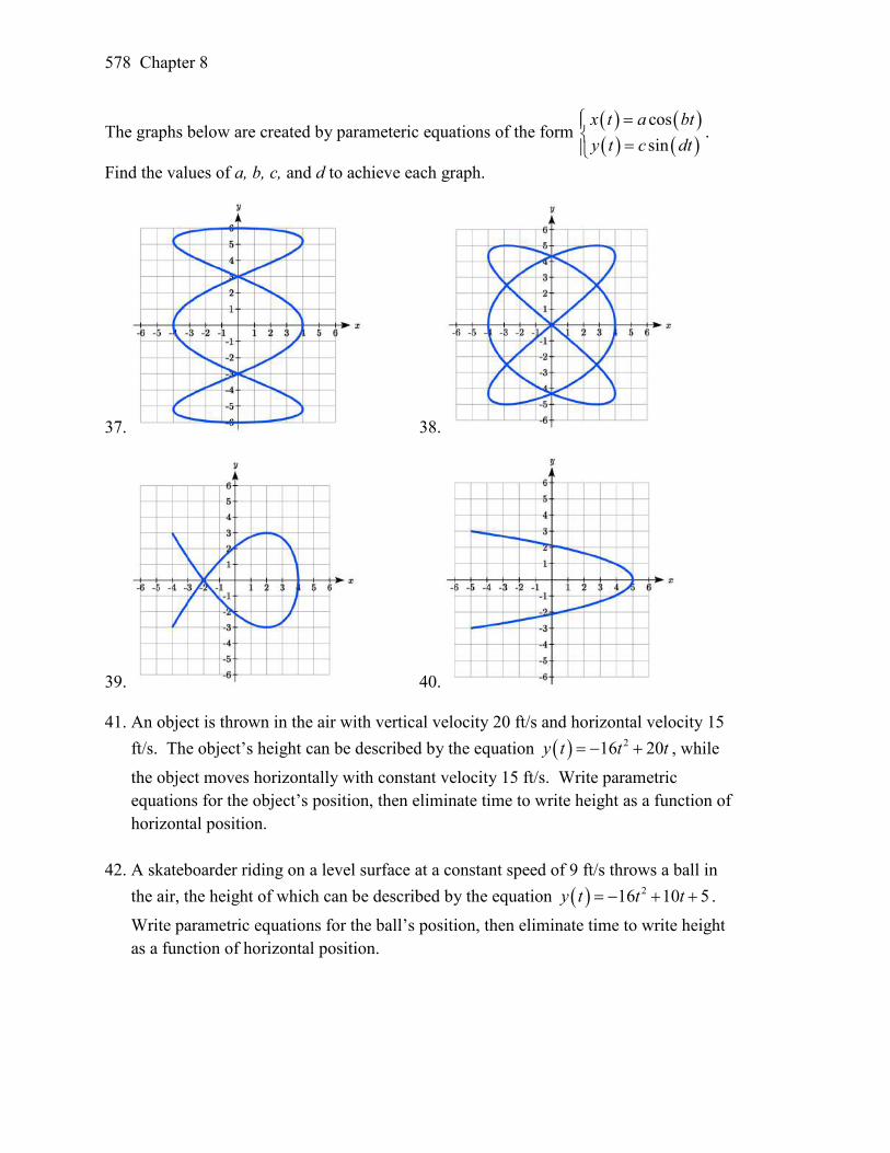
578 Chapter 8
The graphs below are created by parameteric equations of the form ( ) ( )( ) ( )
cossin
x t a bty t c dt
= =
.
Find the values of a, b, c, and d to achieve each graph.
37. 38.
39. 40. 41. An object is thrown in the air with vertical velocity 20 ft/s and horizontal velocity 15
ft/s. The object’s height can be described by the equation ( ) 216 20y t t t= − + , while
the object moves horizontally with constant velocity 15 ft/s. Write parametric equations for the object’s position, then eliminate time to write height as a function of horizontal position.
42. A skateboarder riding on a level surface at a constant speed of 9 ft/s throws a ball in the air, the height of which can be described by the equation ( ) 216 10 5y t t t= − + + .
Write parametric equations for the ball’s position, then eliminate time to write height as a function of horizontal position.

Section 8.6 Parametric Equations 579
43. A carnival ride has a large rotating arm with diameter 40 feet centered 35 feet off the ground. At each end of the large arm are two smaller rotating arms with diameter 16 feet each. The larger arm rotates once every 5 seconds, while the smaller arms rotate once every 2 seconds. If you board the ride when the point P is closest to the ground, find parametric equations for your position over time.
44. A hypocycloid is a shape generated by tracking a fixed
point on a small circle as it rolls around the inside of a larger circle. If the smaller circle has radius 1 and the large circle has radius 6, find parametric equations for the position of the point P as the smaller wheel rolls in the direction indicated.
P
P

664
Chapter 5
Section 5.1
1. 10 3. ( ) ( )2 2 28 10 8x y− + + =
5. ( ) ( )2 27 2 293x y− + + = 7. ( ) ( )2 25 8 1 3x y− + − =
9. 11. (0, 3 5)+ and (0, 3 5)− 13. (1.3416407865, 7.683281573) 15. (-1.07335, 2.8533) 17. 29.87 miles
Section 5.2
1. 3. π 5. 150° 7. 325°
9. 54° 11. 89π 13.
2π
15. 35 miles 17. 8π cm 19. 5.7596 miles 21. 28.6479° 23. 14.1372 cm2 25. 3960 rad/min 630.254 RPM 27. 2.094 in/sec, π/12 rad/sec, 2.5 RPM 29. 75,398.22 mm/min = 1.257 m/sec 31. Angular speed: π/12 rad/hr. Linear speed: 1036.73 miles/hr
30°
70°
-135° 300°
2𝜋𝜋3
7𝜋𝜋4

665
Section 5.3
1. a. III b. II 3. 45
−
5. 4 37
− 7. 558
−
9. a. reference: 45°. Quadrant III. ( ) 2sin 2252
° = − . ( ) 2cos 2252
° = −
b. reference: 60°. Quadrant IV. ( ) 3sin 3002
° = − . ( ) 1cos 3002
° =
c. reference: 45°. Quadrant II. ( ) 2sin 1352
° = . ( ) 2cos 1352
° = −
d. reference: 30°. Quadrant III. ( ) 1sin 2102
° = − . ( ) 3cos 2102
° = −
11. a. reference: 4π . Quadrant III. 5 2sin
4 2π = −
. 5 2cos
4 2π = −
b. reference: 6π . Quadrant III. 7 1sin
6 2π = −
. 7 3cos
6 2π = −
c. reference: 3π . Quadrant IV. 5 3sin
3 2π = −
. 5 1cos
3 2π =
d. reference: 4π . Quadrant II. 3 2sin
4 2π =
. 3 2cos
4 2π = −
13. a. 3 2sin4 2π − = −
3 2cos
4 2π − = −
b. 23 1sin6 2π = −
23 3cos
6 2π =
c. sin 12π − = −
cos 0
2π − =
d. ( )sin 5 0π = ( )cos 5 1π = −
15. a. 23π b. 100° c. 40° d. 5
3π e. 235°
17. a. 53π b. 280° c. 220° d. 2
3π e. 55°
19. (-11.491, -9.642)

666
Section 5.4 1. ( )sec 2θ = , ( )csc 2θ = , ( )tan 1θ = , ( )cot 1θ =
3. ( ) 2 3sec3
θ = − , ( )csc 2θ = , ( ) 3tan3
θ = − , ( )cot 3θ = −
5. ( )sec 2θ = − , ( ) 2 3csc3
θ = , ( )tan 3θ = − , ( ) 3cot3
θ = −
7. a. ( )sec 135 2° = − b. ( )csc 210 2° = − c. ( )tan 60 3° = . d. ( )cot 225 1° =
9. ( ) 7cos4
θ = − , ( ) 4 7sec7
θ = − , ( ) 4csc3
θ = , ( ) 3 7tan7
θ = − , ( ) 7cot3
θ = −
11. ( ) 2 2sin3
θ = − , ( )4
23csc −=θ , ( ) 3sec −=θ , ( )tan 2 2θ = , ( ) 2cot4
θ =
13. ( ) 12sin13
θ = , ( ) 5cos13
θ = , ( ) 13sec5
θ = , ( ) 13csc12
θ = , ( ) 5cot12
θ =
15. a. sin(0.15) = 0.1494 cos(0.15) = 0.9888 tan(0.15) = 0.1511 b. sin(4) = -0.7568 cos(4) = -0.6536 tan(4) = 1.1578 c. sin(70°) = 0.9397 cos(70°) = 0.3420 tan(70°) = 2.7475 d. sin(283°) = -0.9744 cos(283°) = 0.2250 tan(283°) = -4.3315
17. sec( )t 19. tan( )t 21. tan( )t 23. cot( )t 25. ( )2sec( )t
Section 5.5
1. ( ) ( ) ( )
45tan,
41414cos,
41415sin === AAA
( ) ( ) ( )41 41 4sec ,csc ,cot4 5 5
A A A= = =
3. 14, 7 3, 60c b B= = = ° 5. 5.3171, 11.3257, 28a c A= = = ° 7. 9.0631, 4.2262, 25a b B= = = ° 9. 32.4987 ft 11. 836.2698 ft 13. 460.4069 ft 15. 660.35 feet 17. 28.025 ft 19. 143.0427 21. 86.6685

667
Chapter 6
Section 6.1
1. 3. 5. Amp: 3. Period= 2. Midline: y= -4. ( ) ( )3sin 4f t tπ= −
7. Amp: 2. Period= 4π. Midline: y= 1. ( ) 12cos 12
f t t = +
9. Amp: 2. Period= 5. Midline: y= 3. ( ) 22cos 35
f t tπ = − +
11. Amp: 3, Period = 4π , Shift: 4 left, Midline: y = 5
13. Amp: 2, Period = 23π , Shift: 7 right, Midline: y = 4
15. Amp: 1, Period = 12, Shift: 6 left, Midline: y = -3
17. ( ) ( )4sin 15
f x xπ = +
19. ( ) ( )cos 25
f x xπ = +
21. ( ) 50 7sin12
D t tπ = −
23 a. Amp: 12.5. Midline: y = 13.5. Period: 10
b. ( ) 12.5cos 13.55
h t tπ = − +
c. ( )5 26h = meters

668
Section 6.2 1. II 3. I
5. Period: 4π . Horizontal shift: 8 right
7. Period: 8. Horizontal shift: 1 left 9. Period: 6. Horizontal shift: 3 left
11. 13.
15.
17. ( ) 2sec 1 2
f x xπ = −
19. ( ) 2csc 14
f x xπ = +
21. ( )tan 1.5x− = 23. ( )sec 2x− =
25. ( )csc 5x− = 27. ( )csc x−

669
Section 6.3
1. 4π 3.
6π
− 5. 3π
7. 34π 9.
4π 11.
3π
−
13. 1.9823 15. -0.9273 17. 44.427°
19. 4π 21.
6π
− 23. 7102 25.
171
27. 5
25 2x− 29. 19
32 +xx
Section 6.4
1. 5 7,4 4π π 3. 5,
3 3π π 5.
2π 7. 3,
2 2π π
9. 72 , 24 4
k kπ ππ π+ + , where k is an integer
11. 7 112 , 26 6
k kπ ππ π+ + , where k is an integer
13. 2 5 2,18 3 18 3
k kπ π π π+ + , where k is an integer
15. 5 2 7 2,12 3 12 3
k kπ π π π+ + , where k is an integer
17. 5,6 6
k kπ ππ π+ + , where k is an integer
19. 2 5 2,4 3 12 3
k kπ π π π+ + , where k is an integer
21. 4 8k+ , where k is an integer
23. 1 52 , 26 6
k k+ + , where k is an integer
25. 0.2734, 2.8682 27. 3.7603, 5.6645 29. 2.1532, 4.1300 31. 0.7813, 5.5019 33. 0.04829, 0.47531 35. 0.7381, 1.3563 37. 0.9291, 3.0709 39. 1.3077, 4.6923

670
Section 6.5 1. 89c = , A = 57.9946°, B = 32.0054° 3. 1 76b = , A = 27.8181°, B = 62.1819°
5. ( ) ( )6sin 1 42
y x xπ = − +
7. ( ) ( )π50 13cos t 512
D t = − −
9. a. ( ) 129 25cos6
P t tπ = −
b. ( ) 129 25cos ( 3)6
P t tπ = − −
11. 75 degrees 13. 8 15. 2.80869431742 17. 5.035 months
Chapter 7
Section 7.1
1. 7 11,6 6π π 3. 5,
3 3π π
5. 2 83
k+ , and 10 83
k+ , where k is an integer
7. 512
kπ π+ and 712
kπ π+ , where k is an integer
9. 0.1339 10k+ and k106614.8 + , where k is an integer
11. 21.14383
kπ+ and 21.9978
3kπ
+ , where k is an integer
13. 3, , 0.644, 2.4982 2π π 15. 0.056, 1.515, 3.197, 4.647
17. 50, , , 3 3π ππ 19. 5 7 11, , ,
6 6 6 6π π π π
21. 1.183, 1.958, 4.325, 5.100 23. 3 7 11, ,2 6 6π π π
25. 5, ,3 3π ππ 27. 1.823, 4.460
29. 2.301, 3.983, 0.723, 5.560 31. 3.305, 6.120

671
33. 2 4 50, , , , ,3 3 3 3π π π ππ 35. 3 5 70, , , , ,
4 4 4 4π π π ππ
37. 3
4,6
5, 3
2,6
ππππ 39. 0, ,1 .231, 5.052π
41. 5,3 3π π
Section 7.2
1. 2 64+ 3. 2 6
4− −
5. 2 64− 7. 2 6
4+
9. ( ) ( )3 1sin cos2 2
x x− 11. ( ) ( )3 1– cos sin2 2
x x+
13. ( )sec t 15. ( )tan x
17. ( ) ( )( )8 cos 5 cos 27x x− 19. ( ) ( )sin 8 sin 2x x+
21. ( ) ( )2cos 5 cost t 23. ( ) ( )2sin 5 cos 2x x
25. a. 2 1 5 15 2 5 33 4 3 4 12
− − − + − =
b. 5 1 2 15 5 2 153 4 3 4 12
+ − − + =
27. 20.3733
kπ+ and 20.674
3kπ
+ , where k is an integer
29. kπ2 , where k is an integer
31. 47 7
kπ π+ , 3 4
7 7kπ π
+ , 43 3
kπ π+ , and 4
3kππ + , where k is an integer
33. 712
kπ π+ , 1112
kπ π+ , and 4
kπ , where k is an integer
35. 2 13sin( 5.3004)x + or 2 13sin( 0.9828)x −
37. 29sin(3 0.3805x + ) 39. 0.3681, 3.8544
41. 0.7854, 1.8158 43. ( )tan 6t

672
Section 7.3
1. a. 3 732
b. 3132
c. 3 731
3. ( )cos 56°
5. cos(34 )° 7. ( )cos 18x
9. ( )2sin 16x 11. 0, , 2.4189, 3.8643π
13. 0.7297, 2.4119, 3.8713, 5.5535
15. 5 3, , ,6 2 6 2π π π π
17. a. 3
4,3
2, 0,9
16,9
14,9
10,9
8,9
4,9
2 ππππππππ
19. ( )1 cos 10
2x+
21. ( ) ( )xx 32cos8116cos
21
83
+−
23. ( ) ( ) ( ) ( )1 1 1 1cos 2 cos 4 cos 2 cos 416 16 16 16
x x x x− + −
25. a. 1 2 32 7+ b. 1 2 3
2 7− c. 1
7 4 3−
Section 7.4
1. ( )3sin 3 16
y xπ = − −
3. Amplitude: 8, Period: 13
second, Frequency: 3 Hz (cycles per second)
5. ( ) 4019cos 6506 3
P t t tπ = − + +
7. ( ) ( )33cos 900 1.076
tP t tπ = − +

673
9. ( ) ( )10 0.85 cos(36 )tD t tπ= 11. ( ) ( ) ( )17 0.9145 cos 28tD t tπ=
13. a. IV b. III 15. ( )6 4 5sin2
xy xπ = +
17. 3sin 2 72
y xπ = − + +
19. 32
cos218 +
= xy
x π
Chapter 8
Section 8.1
1. 3.
5. 7.
9. β = 68°, a = 14.711, c = 20.138 11. β = 28.096°, γ = 32.904°, c = 16.149
13. Not possible.
15. β = 64.243°, γ = 72.657°, c = 257.328 OR β =115.757°, γ = 21.143°, c = 97.238
17. 19.
21. °=°== 255.86, 545.52,066.2 βαc
70° 50°
10 60°
12.26
11.305
120
6
25°
35° 4.421
9.059
65°
5 6
49.048°
65.952°
6.046
1
40°
25
116.668°
23.222°
11.042
60° 20 28
24.980 43.898° 76.102°
13
11
20
112.620°
30.510°
36.870°

674
23. °=°== 543.32, 457.27,269.11 γβa
25. 177.562 27. 978.515 ft
29. Distance to A: 565.258 ft. Distance to shore: 531.169 ft
31. 529.014 m 33. 173.877 feet
35. 4.642 km, 2.794 km 37. 757.963 ft
39. 2371.129 miles 41. 65.375 cm2
43. 7.72
Section 8.2
1.
−−
27,
237 3. ( )2 2, 2 2−
5. ( )3 2, 3 2− 7. (0,3)
9. 3 3 3,2 2
− −
11. ( 1.248, 2.728)−
13. ( )2 5, 0.464 15. ( )2 13,2.159
17. ( )34,5.253 19. ( )269,4.057
21. ( )θsec3=r 23. ( )( )2
sin4cos
rθθ
=
25. ( )4sinr θ= 27. ( )( ) ( )( )2 2
coscos sin
rθ
θ θ=
−
29. 2 2 3x y y+ = 31. 7 4y x+ =
33. 2x = 35. 2 2 2x y x+ = + 37. A 39. C 41. E 43. C 45. D 47. F
49. 51. 53.

675
55. 57. 59.
61. 63. 65.
Section 8.3 1. 3i 3. 12− 5. 1 3i+ 7. 8 i− 9. 11 4i− + 11. 12 8i− + 13. 30 10i− 15. 11 10i+
17. 20 19. 3 22
i+
21. 3 52 2
i+ 23. 1 1825 25
i− −
25. 1− 27. i 29. ( ) ( )3cos 2 3sin 2 1.248 2.728i i+ = − +
31. 3 3 3i+ 33. 3 2 3 2– –2 2
i
35. 06 ie 37. 324
ie
π
39. 42 2i
eπ
41. 343 2
ie
π
43. 0.54034 ie 45. 2.82010 ie
47. 4.46717 ie 49. 6.086 26 ie
51. 5126
ie
π
53. 7122
ie
π
55. 521024
ie
π
57. 34i
eπ

676
59. 4096 61. 0.788 1.903i+ 63. 1.771 0.322i+ 65. iiii 092.1355.0, 675.0929.0, 675.0929.0, 092.1355.0, 149.125 −−−+−+≈
67. 1 3 1 3 1 3 1 31, , , 1, , 2 2 2 2 2 2 2 2
i i i i+ − + − − − −
Section 8.4 1. 4, 2−
3. The vectors do not need to start at the same point 5. 3v u− 7. 3 2,3 2
9. 6.128, 5.142− − 11. Magnitude: 4, Direction: 90°
13. Magnitude: 7.810, Direction: 39.806°
15. Magnitude: 2.236, Direction: 153.435°
17. Magnitude: 5.385, Direction: 291.801°
19. Magnitude: 7.211, Direction: 236.310°
21. 21,132, 8,1, 2,3 −=−−=−=+ vuvuvu
23. 4.635 miles, 17.764 deg N of E
25. 17 miles. 10.318 miles
27. 4, 11netF = − −
29. Distance: 2.868. Direction: 86.474° North of West, or 3.526° West of North
31. 4.924 degrees. 659 km/hr
33. 4.424 degrees
35. (0.081, 8.602)
37. 21.801 degrees, relative to the car’s forward direction

677
Section 8.5 1. 529.15)75cos(106 =°⋅⋅ 3. 0)0)(4()3)(0( =+− 5. 33)13)(1()10)(2( =+−−
7. °=
− 9034
0cos 1 9. °=
−++
−+− 135)3(142
)3)(4()1)(2(cos2222
1
11. °=
++
+− 04284
)4)(2()8)(4(cos2222
1 13. 0)4)(7())(2( =+k , k = -14
15. 325.6)3(1
)3)(4()1)(8(22
=−+
−−+ 17. 8.10,6.33,1)3(1
)3)(10()1)(6(2
22−=−
−+
−+−
19. The vectors are 3,2 and 2,5 −− . The acute angle between the vectors is 34.509°
21. 14.142 pounds 23. 20,0)10sin(10),10cos(10 −⋅°° , so 34.7296 ft-lbs 25. 277.4350)25cos(12040 =°⋅⋅ ft-lbs
Section 8.6 1. C 3. E 5. F
7.
9. x(t) y(t)
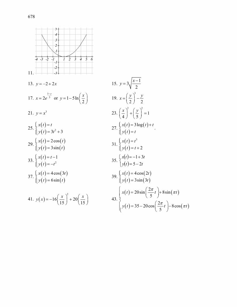
678
11.
13. 2 2y x= − + 15. 13
2xy −
=
17. 1
52y
x e−
= or 1 5ln2xy = −
19.
3
2 2y yx = −
21. 3y x= 23. 2 2
14 5x y + =
25. ( )( ) 23 3
x t ty t t
= = +
27. ( ) ( )( )
3logx t t ty t t
= + =
.
29. ( ) ( )( ) ( )
2cos3sin
x t ty t t
= =
31. ( )( )
3
2x t ty t t
= = +
33. ( )( ) 2
1x t ty t t
= − = −
35. ( )( )
−=+−=
ttyttx
2531
37. ( ) ( )( ) ( )
4cos 36sin
x t ty t t
= =
39. ( ) ( )( ) ( )
4cos 23sin 3
x t ty t t
= =
41. ( )2
16 2015 15x xy x = − +
43.
( ) ( )
( ) ( )
220sin 8sin5
235 20cos 8cos5
x t t t
y t t t
π π
π π
= +
= − −

679
Chapter 9
Section 9.1 1. D 3. B 5. Vertices (0,±5), minor axis endpoints (±2,0), major length = 10, minor length = 4
7. Vertices (±2,0), minor axis endpoints (0,±1), major length = 4, minor length = 2
9. Vertices (±5,0), minor axis endpoints (0,±1), major length = 10, minor length = 2
11. Vertices (0,±4), minor axis endpoints (±3,0), major length = 8, minor length = 6
13. Vertices ( )0, 3 2± , minor axis endpoints ( )2,0± , major length = 6 2 , minor
length = 2 2

680
15. 2 2
116 4x y
+ = 17. 2 2
11024 49
x y+ = 19.
2 2
14 9x y
+ =
21. B 23. C 25. F 27. G 29. Center (1,-2), vertices (6,-2) and (-4,-2), minor axis endpoints (1,0) and (1,-4), major length= 10, minor length = 4
31. Center (-2,3), vertices (-2,8) and (-2,-2), minor axis endpoints (-1,3) and (-3,3), major length = 10, minor length = 2
33. Center (-1,0), vertices (-1,4) and (-1,-4), minor axis endpoints (-1,0) and (3,0), major length = 8, minor length = 4
35. Center (-1,-2), vertices (3,-2) and (-5,-2), minor axis endpoints (-1,0) and (-1,-4), major length = 8, minor length = 4

681
37. Center (2,-1), vertices (2,5) and (2,-7), minor axis endpoints (6,-1) and (-2,-1), major length = 12, minor length = 8
39. ( ) ( )22 1
3 116
yx
+− + = 41.
( ) ( )2 24 31
16 25x y+ −
+ =
43. 2.211083 feet 45. 17 feet 47. 64 feet 49. (±4,0) 51. (-6,6) and (-6,-4)
53. 2 2
19 5x y
+ = 55. 2 2
111 36x y
+ = 57. 2 2
149 24x y
+ = 59. 2 2
14 20x y
+ =
61. 2 2
116 8x y
+ = 63. ( ) ( )2 22 1
112 16
x y+ −+ = 65.
( ) ( )2 23 21
36 11x y− −
+ =
67. ( ) ( )2 23 1
121 25
x y− ++ = 69.
( ) ( )2 21 31
4 5x y− −
+ = 71. ( ) ( )2 22 1
1289 120
x y+ ++ =
73. 31.22 feet 75. 2 2
18640.632025 8638.214
x y+ = 77.
2 2
125 9x y
+ =
79. The center is at (0,0). Since a > b, the ellipse is horizontal. Let (c,0) be the focus on the positive x-axis. Let (c, h) be the endpoint in Quadrant 1 of the latus rectum passing through (c,0).

682
The distance between the focus and latus rectum endpoint can be found by substituting
(c,0) and (c,h) into the distance formula ( ) ( )2 21 2 1 2h x x y y= − + − which yields
( ) ( )2 20h c c h h= − + − = . So h is half the latus rectum distance. Substituting (c,h) into
the ellipse equation to find h gives 2 2
2 2 1c ha b
+ = . Solve for h yields
2 2 2 2 2 2 42 2 2 2 2
2 2 2 2 2 21 c a c a c b bh b b b ba a a a a a
−= − = − = = =
. so
4 2
2
b bha a
= = . The
distance of the latus rectum is 222 bh
a= .
Section 9.2 1. B 3. D 5. Vertices (±2,0), transverse length = 4, asymptotes y = ±5/2x,

683
7. Vertices (0, ±1), transverse length = 2, asymptotes y = ±1/2x,
9. Vertices (±3,0), transverse length = 6, asymptotes y =±1/3x,
11. Vertices (0, ±4), transverse length = 8, asymptotes y =±4/3x
13. Vertices (± 2 ,0), transverse length = 2 2 , asymptotes y =±3x,
15. 2 2
14 9y x
− = 17. 2 2
116 64y x
− = 19. 2 2
19 36x y
− = 21. 2 2
116 16x y
− =
23. C 25. H 27. B 29. A 31. Center (1,-2), vertices (6,-2) and (-4,-2), transverse length = 10, asymptotes y =±2/5(x-1)-2
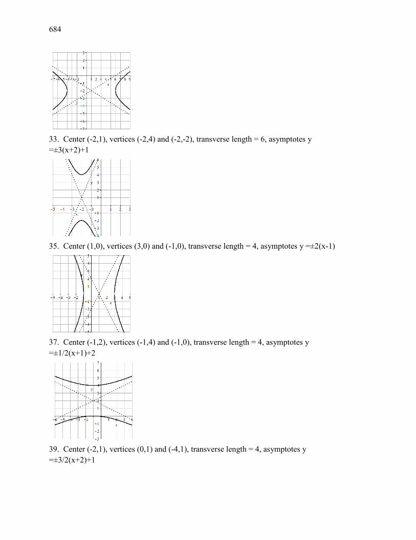
684
33. Center (-2,1), vertices (-2,4) and (-2,-2), transverse length = 6, asymptotes y =±3(x+2)+1
35. Center (1,0), vertices (3,0) and (-1,0), transverse length = 4, asymptotes y =±2(x-1)
37. Center (-1,2), vertices (-1,4) and (-1,0), transverse length = 4, asymptotes y =±1/2(x+1)+2
39. Center (-2,1), vertices (0,1) and (-4,1), transverse length = 4, asymptotes y =±3/2(x+2)+1

685
41. ( ) ( )2 21 4
19 4
y x+ −− = 43.
( ) ( )2 22 11
16 4y x− +
− =
45. Center (0,0), vertices (±1/3,0), transverse length = 2/3, asymptotes y = ±12x
47. Center (-1,1), vertices (-1,3/2) and (-1,1/2), transverse length = 1, asymptotes y = ± 3/2 (x + 1) +1
49. Foci (0,±5) 51. Foci (5,6) and (-3,6) 53. Foci (-4,6) and (-4,-4)
55. 2 2
116 9x y
− = 57. 2 2
1144 25y x
− = 59. 2 2
1225 64x y
− = 61. 2 2
164 36x y
− =
63. ( ) ( )2 22 1
116 9
y x− −− = 65.
( ) ( )2 21 31
25 144x y+ −
− = 67. 2 2
1900 1600x y
− =
69. 2 2
1900 14400.3636x y
− =
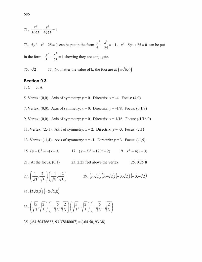
686
71. 2 2
13025 6975
x y− =
73. 2 25 25 0y x− + = can be put in the form 2 2
15 25y x
− = − . 2 2 5 25 0x y− + = can be put
in the form 2 2
15 25y x
− = showing they are conjugate.
75. 2 77. No matter the value of k, the foci are at ( )6,0±
Section 9.3 1. C 3. A 5. Vertex: (0,0). Axis of symmetry: y = 0. Directrix: x = -4. Focus: (4,0) 7. Vertex: (0,0). Axis of symmetry: x = 0. Directrix: y = -1/8. Focus: (0,1/8) 9. Vertex: (0,0). Axis of symmetry: y = 0. Directrix: x = 1/16. Focus: (-1/16,0) 11. Vertex: (2,-1). Axis of symmetry: x = 2. Directrix: y = -3. Focus: (2,1) 13. Vertex: (-1,4). Axis of symmetry: x = -1. Directrix: y = 3. Focus: (-1,5) 15. )3()1( 2 −−=− xy 17. )2(12)3( 2 −=− xy 19. )3(42 −= yx 21. At the focus, (0,1) 23. 2.25 feet above the vertex. 25. 0.25 ft
27.
−−
32,
31,
32,
31 29. ( ) ( ) ( ) ( )2,3,2,3,2,3,2,3 −−−−
31. ( ) ( )8,22,8,22 −
33.
−−
−
−
32,
35,
32,
35,
32,
35,
32,
35
35. (-64.50476622, 93.37848007) ≈ (-64.50, 93.38)

687
Section 9.4 1. e = 3. Directrix: x = 4. Hyperbola. 3. e = 3/4. Directrix: y = -2/3. Ellipse. 5. e = 1. Directrix: x = -1/5. Parabola. 7. e = 2/7. Directrix: x = 2. Ellipse.
9. )cos(51
20θ−
=r 11. )sin(
311
1
θ+=r , or
)sin(33
θ+=r
13. )sin(1
2θ−
=r
15. Hyperbola. Vertices at (-9,0) and (-3,0)
Center at (-6,0). a = 3. c = 6, so b = 27
1279
)6( 22
=−+ yx
17. Ellipse. Vertices at (0,3) and (0,-6)
Center at (0,-1.5). a = 4.5, c = 1.5, 18=b
125.20
)5.1(18
22
=+
+yx
19. Parabola. Vertex at (3,0). p = 3.
)3(122 −−= xy 21. a)
x
y
d(Q,F1) d(Q,F2)
Q=(x,y)
F1 F2
L1 L2
(c,0) (a,0)
x = p

688
b) ( ) pxpxLQd +=−−= )(, 1 , ( ) xpLQd −=2,
c) ( ) ( ) )(,, 11 pxeLQedFQd +== . ( ) ( ) )(,, 22 xpeLQedFQd −==
d) ( ) ( ) epxpepxeFQdFQd 2)()(,, 21 =−++=+ , a constant.
e) At Q = (a, 0), ( ) cacaFQd +=−−= )(, 1 , and ( ) caFQd −=2, , so ( ) ( ) acacaFQdFQd 2)()(,, 21 =−++=+
Combining with the result above, aep 22 = , so eap = .
f) ( ) caFQd −=2, , and ( ) apLQd −=2, ( )( ) e
LQdFQd
=2
2
,, , so e
apca=
−− .
)( apeca −=− . Using the result from (e),
−=− a
eaeca
eaaca −=−
ace =

689

690

691
Index Absolute Value Functions, 149
Graphing, 150 Solving, 151 Solving Inequalities, 152
Ambiguous Case, 501 Amplitude, 399, 402 Angle, 347
Coterminal Angles, 348 Degree, 347 Radian, 351 Reference Angles, 369 Standard Position, 347
Angular Velocity, 356 Annual Percentage Rate (APR), 257 Annual Percentage Yield (APY), 259 Arclength, 350 Arcsine, Arccosine and Arctangent, 423 Area of a Sector, 355 asymptotes of hyperbola, 598 Average Rate of Change, 37 axis of symmetry, 617 Cauchy's Bound, 203 central rectangle, 598 Change of Base, 281, 289 Circles, 338, 518
Area of a Sector, 355 Equation of a Circle, 338 Points on a Circle, 339, 364 Polar Coordinates, 518
Coefficients, 162 Cofunction Identities, 387 Common Log, 279 completing the square, 170 Completing the square, 170 Complex Conjugate, 212, 530 Complex Factorization Theorem, 214 Complex Number, 210, 528 Complex Plane, 529 Component Form, 544 Composition of Functions, 51
Formulas, 54 Tables and Graphs, 52
Compound Interest, 257 Concavity, 43
conic section, 579 Continuous Growth, 260 Correlation Coefficient, 144, 145 Cosecant, 375 Cosecant Function
Domain, 415 Range, 415
Cosine, 363, 385, 398 Cotangent, 375 Cotangent Function
Domain, 416 Period, 416 Range, 416
Coterminal Angles, 348 co-vertices, 580 Damped Harmonic Motion, 492 Decreasing, 40 Degree, 162, 347 Difference of Logs Property, 289 directrix, 617, 630 Domain, 22 Dot Product, 555 Double Angle Identities, 477 Double Zero, 183 Doubling Time, 311 eccentricity, 630 ellipse, 580, 617, 630, 631, 632 Even Functions, 73 Exponential Functions, 249
Finding Equations, 253 Fitting Exponential Functions to Data,
331 Graphs of Exponential Functions, 267 Solving Exponential Equations, 282 Transformations of Exponential
Graphs, 270 Exponential Growth or Decay Function,
251 Exponential Property, 289 Extrapolation, 142 Extrema, 41, 187 Factor Theorem, 196 factored completely, 215 focal length, 617

692 Index
foci, 598 Function, 1
Absolute Value Functions, 149 Composition of Functions, 51 Domain and Range, 22 Exponential Functions, 249 Formulas as Functions, 8 Function Notation, 3 Graphs as Functions, 6 Horizontal Line Test, 7 Inverse of a Function, 93 Linear Functions, 101, 103 Logarithmic Functions, 277 One-to-One Function, 2 Parametric Functions, 564 Periodic Functions, 395 Piecewise Function, 29 Polar Functions, 517 Power Functions, 159 Quadratic Functions, 167 Radical Functions, 239, 240 Rational Functions, 218, 221 Sinusoidal Functions, 397 Solving & Evaluating, 5 Tables as Functions, 4 Tangent Function, 413 Vertical Line Test, 7
Fundamental Theorem of Algebra, 213 Half-Angle Identities, 483 Half-Life, 308 Horizontal Asymptote, 219, 224 Horizontal Intercept, 118 Horizontal Line Test, 7 Horizontal Lines, 119 hyperbola, 598 Imaginary Number, 210, 528
Complex Conjugate, 212, 530 Complex Number, 210, 528 Complex Plane, 529 Polar Form of Complex Numbers, 531
Increasing, 40 Inflection Point, 43 Intercepts, 173, 181, 182, 186, 225
Graphical Behavior, 182 Writing Equations, 186
Interpolation, 142
Interval Notation, 24 Union, 24
Inverse of a Function, 93 Properties of Inverses, 96
Inverse Properties, 289 Inversely Proportional, 218 Inversely Proportional to the Square, 218 Inverses, 239 irreducible quadratic, 215 Law of Cosines
Generalized Pythagorean Theorem, 503
Law of Sines Ambiguous Case, 501
Leading Coefficient, 162 Leading Term, 162 Least-Square Regression, 143 Limaçons, 519 Linear Functions, 101, 103
Fitting Linear Models to Data, 141 Graphing, 114 Horizontal Intercept, 118 Horizontal Lines, 119 Least-Square Regression, 143 Modeling, 129 Parallel Lines, 120 Perpendicular Lines, 120 Veritcal Lines, 119 Vertical Intercept, 115
Linear Velocity, 356 Lissajous Figure, 567 Local Maximum, 41 Local Minimum, 41 Logarithmic Functions, 277
Change of Base, 281, 289 Common Log, 279 Difference of Logs Property, 289 Exponential Property, 280, 289 Graphs of Logarithmic Functions, 300 Inverse Properties, 277, 289 Logarithmic Scales, 314 Log-Log Graph, 329 Moment Magnitude Scale, 318 Natural Log, 279 Orders of Magnitude, 317 Semi-Log Graph, 329
693
Sum of Logs Property, 289 The Logarithm, 277 Transformations of the Logarithmic
Function, 302 Log-Log Graph, 329 Long Division, 194 Long Run Behavior, 161, 163, 219 major axis, 580 Mathematical Modeling, 101 Midline, 400, 402 minor axis, 580 Model Breakdown, 143 Moment Magnitude Scale, 318 multiplicity, 183 Natural Log, 279 Negative Angle Identities, 454 Newton's Law of Cooling, 313 Nominal Rate, 257 oblique asymptote, 230 Odd Functions, 73 One-to-One Function, 2, 7 Orders of Magnitude, 317 orthogonal, 557 Parallel Lines, 120 Parametric Functions, 564
Converting from Parametric to Cartesian, 568
Lissajous Figure, 567 Parameterizing Curves, 570
Period, 395, 402 Periodic Functions, 395
Period, 395 Sinusoidal, 397
Perpendicular Lines, 120 Phase Shift, 406 Piecewise Function, 29 Polar Coordinates
Converting Points, 515 Polar Form of a Conic, 630 Polar Functions, 517
Converting To and From Cartesian Coordinates, 520
Limaçons, 519 Polar Form of Complex Numbers, 531 Roses, 519
Polynomial, 162
Coefficients, 162 Degree, 162 Horizontal Intercept, 183, 186 Leading Coefficient, 162 Leading Term, 162 Long Division, 194 Solving Inequalities, 184 Term, 162
Power Functions, 159 Characterisitcs, 160
Power Reduction Identities, 483 Product to Sum Identities, 468 Projection Vector, 559 Pythagorean Identity, 364, 379
Alternative Forms, 379, 454, 456 Pythagorean Theorem, 337 Quadratic Formula, 175 Quadratic Functions, 167
Quadratic Formula, 175 Standard Form, 169, 170 Transformation Form, 169 Vertex Form, 169
Radian, 351 Radical Functions, 239, 240 Range, 22 Rate of Change, 36
Average, 37 Using Function Notation, 38
Rational Functions, 218, 221 Intercepts, 225 Long Run Behavior, 223
Rational Roots Theorem, 204 Reciprocal Identities, 454 Reference Angles, 369 Remainder Theorem, 196 roots, 164 Roses, 519 Scalar Product, 555 Secant, 375 Secant Function
Domain, 415 Range, 415
Semi-Log Graph, 329 Set-Builder Notation, 24 Short Run Behavior, 164, 167, 173, 181,
219

694 Index
Sign of the Dot Product, 558 Sine, 363, 385, 398 Single Zero, 183 Sinusoidal Functions, 397
Amplitude, 399, 402 Damped Harmonic Motion, 492 Midline, 400, 402 Modeling, 443 Period, 395, 402 Phase Shift, 406 Solving Trig Equations, 437
slant asymptote, 230 Slope, 103, 104, 115
Decreasing, 103 Increasing, 103
Standard Form, 169, 170 Standard Position, 347 Sum and Difference Identities, 461 Sum of Logs Property, 289 Sum to Product Identities, 469 synthetic division, 198 Tangent, 375, 385 Tangent Function, 413
Domain, 413 Period, 413 Range, 413
Term, 162 The Logarithm, 277 Toolkit Functions, 11
Domains and Ranges of Toolkit Functions, 27
Transformation Form, 169 Transformations of Functions, 64
Combining Horizontal Transformations, 79
Combining Vertical Transformations, 79
Horizontal Reflections, 71 Horizontal Shifts, 67 Horizontal Stretch or Compression, 77 Vertical Reflections, 71 Vertical Shifts, 65 Vertical Stretch or Compression, 75
transverse axis, 598 Trigonometric Identities, 376
Alternative Forms of the Pythagorean Identity, 379, 454, 456
Cofunction Identities, 387 Double Angle Identities, 477 Half-Angle Identities, 483 Negative Angle Identities, 454 Power Reduction Identities, 483 Product to Sum Identities, 468 Pythagorean Identity, 364 Reciprocal Identities, 454 Sum and Difference Identities, 461 Sum to Product Identities, 469
Trigonometry Cosecant, 375 Cosine, 363, 385, 398 Cotangent, 375 Right Triangles, 385, 597 Secant, 375 Sine, 363, 385, 398 SohCahToa, 385 Solving Trig Equations, 437 Tangent, 375, 385 The Pythagorean Theorem, 337 Unit Circle, 369
Triple Zero, 183 Unit Circle, 369 Vector, 541, 544
Adding Vectors Geometrically, 542 Adding, Subtracting, or Scaling
Vectors in Component Form, 547 Geometrically Scaling a Vector, 543
Vertex, 167, 169 Vertex Form, 169 Vertical Asymptote, 219, 222 Vertical Intercept, 115 Vertical Line Test, 7 Vertical Lines, 119 Vertices, 580, 598, 617 Work, 560 zeros, 164


