Adaptive numerical schemes for a parabolic problem with blow-up

DEPARTAMENTO DE MATEMÁTICA DOCUMENTO DE TRABAJO

“Adaptive Numerical Schemes for a Parabolic Problem with Blow –Up”

Raúl Ferreira, Pablo Groisman y Julio D. Rossi

D.T.: N° 28 Octubre 2002

Vito Dumas 284, (B1644BID) Victoria, Pcia. de Buenos Aires, Argentina Tel: 4725-7053 Fax: 4725-7010

Email: [email protected]

ADAPTIVE NUMERICAL SCHEMES FOR APARABOLIC PROBLEM WITH BLOW-UP

RAUL FERREIRA, PABLO GROISMAN AND JULIO D. ROSSI

Abstract. In this paper we present adaptive procedures for thenumerical study of positive solutions of the following problem,

ut = uxx (x, t) ∈ (0, 1)× [0, T ),ux(0, t) = 0 t ∈ [0, T ),ux(1, t) = up(1, t) t ∈ [0, T ),u(x, 0) = u0(x) x ∈ (0, 1),

with p > 1. We describe two methods, the first one refines themesh in the region where the solution becomes bigger in a preciseway that allows us to recover the blow-up rate and the blow-up setof the continuous problem. The second one combine the ideas usedin the first one with the moving mesh methods and moves the lastpoints when necessary. This scheme also recovers the blow-up rateand set. Finally we present numerical experiments to illustrate thebehavior of both methods.

1. Introduction.

In this paper we deal with numerical approximations for the followingproblem,

(1.1)

ut = uxx (x, t) ∈ (0, 1)× [0, T ),ux(0, t) = 0 t ∈ [0, T ),ux(1, t) = up(1, t) t ∈ [0, T ),u(x, 0) = u0(x) x ∈ (0, 1).

We assume that u0 is positive and compatible in order to have a regularsolution. If p > 1 it is well known that every positive solution becomesunbounded in finite time, a phenomena that is known as blow-up. If Tis the maximum time of existence of the solution u then

limtT

‖u(·, t)‖∞ = +∞,

see [24], [28], [31] and also [17], [23], [27], [30] for general references onblow-up problems. For (1.1) it is proved in [13], [18] that the blow-up

1991 Mathematics Subject Classification. 35B40, 35K20, 65M50, 65N50.Key words and phrases. numerical blow-up, heat equation, nonlinear boundary

conditions, adaptive mesh.1

2 R. FERREIRA, P. GROISMAN AND J.D. ROSSI

rate is given by,

‖u(·, t)‖L∞ ∼ (T − t)−1

2(p−1) .

The blow-up set, B(u), i.e., the set of points x ∈ [0, 1] where u(x, t)becomes unbounded, is given by,

B(u) = 1.This phenomena is called single point blow-up, see [21].

Here we are interested in numerical approximations of (1.1). Sincethe solution u develops a singularity in finite time, it is an interestingquestion what can be said about numerical approximations of this kindof problems. For previous work on numerical approximations of blow-ing up solutions we refer to [1], [2], [6], [7], [10], [11], [15], [22], [25],[26] the survey [5] and references therein. For approximations of (1.1)we refer to [3], [4] and [14]. Those papers deal with the behaviour ofa semidiscrete numerical approximation in a fixed mesh of size h. It isobserved there that significant differences appear between the continu-ous and the discrete problems. First, it is proved that positive solutionsof the numerical problem blow up if and only if p > 1, see [14], thisis the same blow-up condition that holds for the continuous problem.Next, it is shown in [3] and [4] that the blow-up rate for the numericalapproximation, U , is given by

‖U(t)‖∞ ∼ (Th − t)−1

p−1 .

Therefore the blow-up rate does not coincide with the expected for thecontinuous problem. Concerning the blow-up set it holds,

B(U) = [1− Lh, 1] if p > 1,

see [4], [16]. The constant L depends only on p, L is the only integerthat verifies

L + 1

L< p ≤ L

L− 1.

Hence the numerical blow-up set can be larger than a single point,x = 1, but as L does not depend on h,

B(U) → B(u), as h → 0.

Collecting all these results, we observe that when computing numer-ical approximations of a blow-up problem with a fixed mesh significantdifferences appear concerning the behaviour of the numerical and thecontinuous solutions. For this problem the blow-up rate and the blow-up set can be different. We conclude that the usual methods witha fixed grid are not well suited for the problem under consideration.

ADAPTIVE NUMERICAL SCHEMES 3

Therefore an adaptive mesh refinement is necessary. Some referencesthat use adaptive numerical methods are [3], [7] and [10].

In this paper we introduce two adaptive methods that give the rightblow-up rate and the exact blow-up set. Our main interest is to providerigorous proofs of these facts.

The first method, that we will call adding points method, is based ona semidiscretization in space and adds points near the boundary, x = 1,when the numerical solution becomes large. This adaptive procedureleads to a non-uniform mesh that concentrates near the singularity andgives the precise blow-up rate and set.

The second one, that we will call moving points method, also usesa semidiscretization in space but this time we move the last K pointsnear the boundary when the numerical solution becomes large. Thenumber of moving points, K, depends only on the exponent p, in factwe will choose K = [1/(p − 1)]. This procedure is inspired in themoving mesh algorithms developed in [8], [9], [10], [20]. In our casewe take advantage of the a priori knowledge of the spatial locationof the singularity at x = 1 and instead of moving the whole meshcontinuously as time evolves, we concentrate only the last K points nearthe boundary, leaving the rest of the mesh fixed. This allows us to usea unified approach to analyze rigorously both schemes simultaneously.One advantage of this moving procedure is keeping the size of the ODEproblem to be solved constant in time, while the adding points methodsenlarges the number of equations as time evolves.

Both numerical schemes are based on the scale invariance of theheat equation in the half line with the nonlinear boundary conditionplaced at x = 0, −ux(0, t) = up(0, t). If u(x, t) is a solution then

uλ(x, t) = λ1

2(p−1) u(λ12 x, λt) also is a solution. In [18] it is proved that

there exists a self-similar blowing up solution in the half-line of theform

uS(x, t) = (T − t)−1

2(p−1) ϕ(ξ), ξ = x(T − t)−12 .

For an explicit form of the profile ϕ, see [18]. This solution uS(x, t)gives the behaviour near the blow-up time T for solutions of (1.1) inthe following sense

(1.2) u(x, t) ∼ (T − t)−1

2(p−1) ϕ(ξ),

for x = 1 − ξ(T − t)1/2, |ξ| ≤ C. So the behavior near the blow-uppoint (1, T ) is given by the self-similar solution in the half-line. Thenumerical schemes presented here use this fact to add or move pointsnear x = 1 trying to reproduce the scaling invariance in the half-line.


The main goal of this paper is to present rigorous estimates for bothmethods simultaneously showing that they give the right blow-up rateand set. Our result reads as follows and holds for the method that addspoints as well as for the method that moves the last points.

Theorem 1.1. Let u be an increasing in x, smooth solution of (1.1) anduh be the numerical solution obtained by any of the adaptive schemesdescribed in section 2. Then, for every τ > 0, the numerical solutionuh converges to the continuous one uniformly in [0, 1] × [0, T − τ ], infact there exists a constant C = C(τ) such that

‖u− uh‖L∞([0,1]×[0,T−τ ]) ≤ Ch32 .

The numerical solution uh blows up if and only if p > 1 in the sensethat there exists a finite time Th with

limtTh

uh(1, t) = +∞.

This numerical blow-up time converges to the continuous one whenh → 0, in fact there exist α > 0 and C > 0 such that

|Th − T | ≤ Chα.

Moreover, the numerical blow-up rate is given by

limtTh

(Th − t)1

2(p−1)‖uh(·, t)‖∞ = Γ = ϕ(0)

and the numerical blow-up set is

B(uh) = 1.Organization of the paper: In section 2 we describe the numericaladaptive procedures. In sections 3 to 6 we develop the proofs of themain result, Theorem 1.1. To begin the analysis we prove in section 3that numerical approximations converge uniformly in sets of the form[0, 1]× [0, T − τ ]. In section 4 we prove that the scheme reproduces theblow-up rate. In section 5 we find the numerical blow-up set that co-incides with the continuous one. In section 6 we prove that the numer-ical blow-up time converges to the continuous one. Finally, in section7 we present some numerical experiments comparing the performanceof both methods and make a few comments on possible extensions ofthe ideas developed here to several space dimensions. We leave for theAppendix the proof of a technical result needed in section 6.


2. Adaptive numerical schemes

In this section we present the numerical methods. We consider asemidiscrte scheme, that is, we discretize the space variable, keeping tcontinuous. For the spatial discretization we propose piecewise linearfinite elements with mass lumping.

Consider a partition (that can be non-uniform), x1, ..., xN+1 of (0, 1)of size h (h = max(xi − xi−1)) and its associated standard piecewiselinear finite element space Vh. Let ϕj1≤j≤N be the usual Lagrangebasis of Vh. The semidiscrete approximation uh(t) ∈ Vh obtained bythe finite element method with mass lumping is defined by:∫ 1

0

(u′hv)Idx +

∫ 1

0

(uh)xvxdx = up(1, t)v(1, t), ∀v ∈ Vh,∀t ∈ (0, T )

where the superindex I denotes the Lagrange interpolation. We denotewith U(t) = (u1(t), . . . , uN+1(t)) the values of the numerical approxi-mation at the nodes xk, at time t. Writing,

uh(t) =N∑

j=1

uj(t)ϕj,

a simple computation shows that U(t) satisfies the system of ordinarydifferential equations (see [12]):

MU ′(t) = −AU(t) + BUp(t),U(0) = uI

0,

where M is the mass matrix obtained with lumping, A is the stiffnessmatrix and uI

0 is the Lagrange interpolation of the initial data, u0.

Adding points method.

First, let us describe a method that adds points near the boundary.Let us pay special attention to the numerical solution at the point x = 1(at this point is where the continuous solution develops the singularity).Writing the equation satisfied by uN+1 explicitly we obtain the followingODE,

u′N+1(t) =2

h2N

(uN(t)− uN+1(t)) +2

hN

upN+1(t),

where hN = 1− xN . Now, let us describe our adaptive procedure. Aswe want the numerical blow-up rate to be

uh(1, t) ∼ (Th − t)−1

2(p−1)

we impose that the last node uN+1(t) = uh(1, t) satisfies

(2.1) c1u2p−1N+1 (t) ≤ u′N+1(t) ≤ c2u

2p−1N+1 (t).


Imposing (2.1) is equivalent to,

(2.2) c1u2p−1N+1 (t) ≤ 2

h2N

(uN(t)− uN+1(t)) +2

hN

upN+1(t) ≤ c2u

2p−1N+1 (t).

As it is proved in [14] that the scheme with a fixed mesh blows up atthe last node, we have that

R(t; hN) =

2h2

N(uN(t)− uN+1(t)) + 2

hNup

N+1(t)

u2p−1N+1 (t)

→ 0 as t increases.

Let t1 be the first time such that R(t; hN) = c1, that is the first timewhere R(t; hN) meets the tolerance c1. At that time t1 we add a pointz between xN and xN+1 = 1 to the mesh and give the value of uh(z, t1)such that the slope of the line between (z, uh(z, t1)) and (1, uh(1, t1))is the same as the slope between (xN , uh(xN , t1)) and (1, uh(1, t1)), seeFigure 1.

Figure 1.

Hence we have a new value for the length of the last interval, [z, 1],

hN,1 = 1− z < hN = 1− xN .

We remark that uh(z, t1) = uz(t1) satisfies,

1

hN

(uN(t1)− uN+1(t1)) =1

hN,1

(uz(t1)− uN+1(t1)).


Let us see what happens with R(t1; hN,1).

R(t1; hN,1) =

2h2

N,1(uz(t1)− uN+1(t1)) + 2

hN,1up

N+1(t1)

u2p−1N+1 (t1)

=

2hN,1

(uz(t1)− uN+1(t1)) + 2upN+1(t1)

hN,1 u2p−1N+1 (t1)

=2

hN(uN(t1)− uN+1(t1)) + 2up

N+1(t1)

hN,1 u2p−1N+1 (t1)

=hN

hN,1

R(t1; hN) =hN

hN,1

c1 > c1.

Therefore with this new mesh x1, ..., xN , z, xN+1 we have that

R(t1; hN,1) > c1,

and we can apply the method with initial data uh(x, t1) in the newmesh to continue. This gives a solution uh that verifies (2.2) in a timeinterval [t1, t2] where at time t2, the function R(t2; hN,1) reaches thetolerance c1. At that time t2 we have to add another point in the lastinterval. As before this increases R(t2; hN,2) and we can continue withinitial data uh(x, t2) in a new mesh that is the old one plus the pointthat we have added near the boundary x = 1. This procedure generatesan increasing sequence of times ti and a decreasing sequence hi = hN,i,at which the tolerance R(ti; hi) = c1 is reached, a sequence of addedpoints accumulating at x = 1 and a numerical solution uh(x, t).

It remains to be more concrete on the election of the sequence hi, c1

and c2. In fact if we take,

c1 = Γ−2(p−1)(2(p− 1))−1,

and hi and c2 such that

(2.3)hi

hi+1

→ 1 and c2 = c2(t) ∼ c1,

integrating (2.1) we get that

Γ(Th − t)−1

2(p−1) ≥ uN+1(t) = max uh(·, t)

≥(

2(p− 1)

∫ Th

t

c2(s) ds

)− 12(p−1)

,


Hence, as t Th,

uN+1(t) = max uh(·, t) ∼ Γ(Th − t)−1

2(p−1) ,

and we have recovered the continuous asymptotic behaviour (1.2). Sowe want that hi and c2 verify (2.3). On the other hand, as we havementioned in the introduction, the continuous problem verifies that

u(x, t) ∼ (T − t)−1

2(p−1) ϕ(ξ)

for x = 1 − ξ(T − t)1/2 ∼ C(u(1, t))−(p−1). In order to recover thisself-similar scaling we choose hi such that

hi+1(uN+1(ti))p−1 =

2

c1

− A

uN+1(ti),

this choice make

c2 ∼ c1

(1

1− c1A2uN+1(ti)

),

and hence,

1− xN = hi+1 ∼ 2

c1

(uN+1(ti))−(p−1) ∼ C(Th − t)1/2.

This procedure gives an approximation of the curve x = 1−ξ(T −t)1/2.Notice that if hi+1 and c2 are given as above, relations (2.3) hold. Sowe recover the self-similar behavior (1.2).

Moving points method.

As we mentioned in the introduction we may use a procedure in-spired in the moving mesh method. Let us describe briefly the mainingredients of such type of schemes, referring to [10] for details. Fol-lowing [10], the numerical solution is defined on a new mesh xi(t) thatis obtained from a differentiable mesh transformation x = x(ξ, t) withxi(t) = x(i/N, t). For this approach a new partial differential equa-tion for x(ξ, t) is solved numerically simultaneously with the originalequation for u(x, t) imposing a self-similar invariance on the resultingproblem. In our case we impose that the blowing up end, xN = 1, isfixed and move the rest of the points according to the previously de-scribed procedure, obtaining a 2N system of ODE to be solved. Thereare various ways to move the meshes, we refer to [10] for the details.

This type of procedure may loose some accuracy as it concentratesthe points near x = 1 as the solution becomes bigger leaving ”holes”near the other end x = 0. Our strategy is to take advantage of thefact that we know a priori that the singular set is x = 1 and hence toreproduce the main features of the continuous solution: the blow-up


rate, the structure of the solution near the blow-up time (approximateself-similar behavior) and the blow-up set. We only need to move thelast K points near x = 1. In fact we use the ideas developed in theadding points method to move the points not in a continuous way butat certain times where R(t, hN) = c1.

Next we describe our moving points method that, as we mentionedbefore, instead of adding a point when R(t, hN) = c1, moves the lastK points near the boundary x = 1.

Let us begin with a mesh composed by two types of nodes, a uniformmesh of size h = 1/N (the fact that this mesh is uniform is not essentialfor our analysis) and K nodes placed between xN = (N − 1)h andxN+1 = 1, that we are going to move when appropriate. The numberof moving nodes, K, depends only on p, we choose K = [1/(p − 1)].The motivation for this choice of K comes from the desired localizationof the blow-up set at x = 1, see Section 5. Let us call 0 = x1 < .... <xN < xN+1 = 1 the fixed mesh and xN < y1 < .... < yK < xN+1 = 1the moving nodes. As before, we use a semidiscretization in space,using the mesh composed by the xi and the yi together, and arrive toa system of ODE

MU ′(t) = −AU(t) + BUp(t),U(0) = uI

0.

Again, we pay special attention to the numerical solution at the pointx = 1. Writing the equation satisfied by uN+1 explicitly we obtain thefollowing ODE,

u′N+1(t) =2

h2N

(uN(t)− uN+1(t)) +2

hN

upN+1(t),

where hN = 1− yK . Now we proceed as follows to obtain an adaptiveprocedure: as before we want the numerical blow-up rate to be

uh(1, t) ∼ (Th − t)−1

2(p−1) .

Hence we impose that the last node uN+1(t) = uh(1, t) satisfies (2.1),this is equivalent to

(2.4) c1u2p−1N+1 (t) ≤ 2

h2N

(uN(t)− uN+1(t)) +2

hN

upN+1(t) ≤ c2u

2p−1N+1 (t).

In this case hN = 1− yK . We have that

R(t; hN) =

2h2

N(uN(t)− uN+1(t)) + 2

hNup

N+1(t)

u2p−1N+1 (t)

→ 0 as t increases.


Let t1 be the first time such that R(t; hN) = c1, that is the first timewhere R(t; hN) meets the tolerance c1.

We remark that our criteria to stop and modify the mesh is the sameas before.

Assume, to simplify the exposition, that K = 1, that is, we only haveone moving point, yK between xN−1 and xN = 1. At that time t1 wemove the point yK between xN and xN+1 = 1 to the point z and give thevalue of uh(z, t1) such that the slope of the line between (z, uh(z, t1))and (1, uh(1, t1)) is the same as the slope between (xN , uh(xN , t1)) and(1, uh(1, t1)), see Figure 2.

PSfrag replacements

xN−1yKyK xN = 1

Figure 2.

Hence, exactly as before, we have a new value for the length of the lastinterval, [z, 1],

hN,1 = 1− z < hN = 1− yK .

As before, R(t1; hN,1) verifies,

R(t1; hN,1) =hN

hN,1

R(t1; hN) =hN

hN,1

c1 > c1.

Therefore with this new mesh x1, ..., xN , z = yK , xN+1 we have that

R(t1; hN,1) > c1,

and we can apply the method with initial data uh(x, t1) in the newmesh to continue.

We remark that the number of nodes does not increase. We haveonly moved the node yK from its previous position to its new position,z. Hence, the size of the ODE system does not increase.

This gives us a solution uh that verifies (2.2) in a time interval [t1, t2]where at time t2, the function R(t2; hN,1) reaches the tolerance c1. Atthat time t2 we have to move again the moving point, yK , in the lastinterval. As before this increases R(t2; hN,2) and we can continue with


initial data uh(x, t2). This procedure generates an increasing sequenceof times ti and a decreasing sequence hi = hN,i, at which the toleranceR(ti; hi) = c1 is reached, a sequence of moving points accumulating atx = 1 and a numerical solution uh(x, t). It remains to be more concreteon the election of the sequence hi, c1 and c2. In fact if we take, exactlyas before,

c1 = Γ−2(p−1)(2(p− 1))−1,

and hi such that

hi

hi+1

→ 1 and c2 = c2(t) ∼ c1,

we get that

uN+1(t) = max uh(·, t) ∼ Γ(Th − t)−1

2(p−1) ,

and we have recovered the continuous asymptotic behavior (1.2). Onthe other hand, to recover the self-similar behavior, we choose hi as inthe adding points method, that is such that

hi+1(uN+1(ti))p−1 =

2

c1

− A

uN+1(ti),

so

c2 ∼ c1

(1

1− c1A2uN+1(ti)

).

Hence,

1− yK = hi+1 ∼ 2

c1

(uN+1(ti))−(p−1) ∼ C(Th − t)1/2.

This procedure gives an approximation of the curve x = 1−ξ(T −t)1/2.Notice that if hi+1 and c2 are given as above, relations (2.3) hold. Sowe recover the self-similar behavior (1.2).

In case we have K > 1 we proceed in the same way, but in this casewe have to move K points near xN+1 = 1. Observe that the scalingfactor that we are using places yK at z, we move the rest of the pointslying between xN and 1 such that the mesh remains uniform in theinterval [y1, 1]. This imposes on yj, j = 1, . . . , K the same behaviordescribed above for yK .

Let us remark that the criteria that we use to modify the mesh isthe same in the adding points method and in the moving points method.This allows us to make a unified approach in the course of the proofscontained in the following sections.


3. Convergence of the numerical schemes

In this section we prove a uniform convergence result. We use ideasfrom [14] and we include the arguments here to make the paper self-contained. For any τ > 0 we want that uh → u (when h → 0) uniformlyin [0, 1] × [0, T − τ ]. This is a natural requirement since on such aninterval the exact solution is regular.

In particular, uniform convergence can be obtained by using standardinverse inequalities. In the following Theorem we give a proof of theL2 convergence for a problem like (1.1) considering mass lumping. Asa corollary, we will obtain uniform convergence for problem (1.1).

Theorem 3.1. Let u be the solution of (1.1) and let uh its semidiscreteapproximation obtained by any of the adaptive schemes described inSection 2. If u ∈ C2,1([0, 1] × [0, T − τ ]) for some τ > 0 then, thereexists a constant C depending on τ such that:

‖u− uh‖L∞([0,T−τ ],L2) ≤ Ch2.

Proof. We fix our attention on the convergence of the method in a timeinterval of the form [ti, ti+1], that is between two consecutive refinementtimes. Next we will show that this is enough for our purposes. Let usbegin by t ∈ (0, t1).

In this proof we use the notation L2 = L2((0, 1)) that refers to theL2 norm in the x variable for each t (we will use analogous notationsfor other norms below) and u′ for the derivative respect to time, ut.

As u is a solution of (1.1) it satisfies∫ 1

0

u′v +

∫ 1

0

uxvx = up(1, t)v(1, t) ∀v ∈ H1.

The numerical scheme is equivalent to∫ 1

0

((uh)′v)I +

∫ 1

0

uxvx = uph(1, t)v(1, t) ∀v ∈ Vh.

Hence we have that e = u− uh satisfies the following error equation,∫ 1

0

(e′v)I dx +

∫ 1

0

exvx dx = (up − uph)(1, t)v(1, t) +

∫ 1

0

((u′v)I − u′v) dx

for all v ∈ Vh. Writing

e = u− uh + uI − uI = u− uI + η

and using known error estimates for Lagrange interpolation it rest toestimate η = uI − uh.


First, it is easy to see that,∫ 1

0

(u− uI)xvx = 0 ∀v ∈ Vh,

and therefore, replacing in the error equation we have an equation forη,

∫ 1

0

(η′v)I+

∫ 1

0

ηxvx = (up(1, t)− uph(1, t))v(1, t)

+

∫ 1

0

((u′v)I − u′v)−∫ 1

0

((u′ − (uI)′)v)I ∀v ∈ Vh.

In particular if we choose v = η ∈ Vh we obtain

1

2

d

dt(

∫ 1

0

(η2)I) +

∫ 1

0

(ηx)2 = (up − up

h)(1, t)η(1, t)

+

∫ 1

0

((u′η)I − u′η) = I + II.

First, let us estimate I.

|I| = |(up(1, t)− uph(1, t))η(1, t)| = ∣∣((uI)p(1, t)− up

h(1, t))η(1, t)∣∣ .

Hence we get that

|I| ≤ C|η(1, t)|2.Using the well known inequality,

|η(1, t)|2 ≤ (C +C

ε)‖η‖2

L2((0,1)) + ε‖ηx‖2L2((0,1)),

we have that

|I| ≤ Cε‖η‖2L2((0,1)) + ε‖ηx‖2

L2((0,1)).

In order to get a bound for II we decompose it in the following form,

II =

∫ 1

0

((u′η)I−u′η) dx =

∫ 1

0

((u′η)I−(u′)Iη) dx+

∫ 1

0

((u′)Iη−u′η) dx.

We proceed as before, for each subinterval Ij of the partition we knowthat,

‖((u′)Iη)I − (u′)Iη‖L1(Ij) ≤ Ch2‖((u′)Iη)xx‖L1(Ij)

≤ Ch2‖((u′)I)xηx‖L1(Ij)


because (u′)I and η are linear over Ij. Hence, summing over all theelements Ij and using that ‖((u′)I)x‖L2 ≤ C‖u′‖H1 we obtain,

∫ 1

0

((u′η)I− (u′)Iη) dx ≤ Ch2

∫ 1

0

|((u′)I)x||ηx| dx

≤ Ch2‖((u′)I)x‖L2((0,1))‖ηx‖L2 ≤ Ch4‖u′‖2H1 + 1

4‖ηx‖2

L2 .

It rests to estimate the second summand of II. We have,∫ 1

0

((u′)I− u′)η dx ≤ ‖(u′)I − u′‖L2‖η‖L2

≤ ‖(u′)I − u′‖2L2 + ‖η‖2

L2 ≤ Ch4‖u′‖2H2 + ‖η‖2

L2 .

Collecting all the previous bounds we obtain,

1

2

d

dt

∫ 1

0

(η2)I+

∫ 1

0

|ηx|2 ≤ Cε‖η‖2L2((0,1)) + Cε‖ηx‖2

L2((0,1))

+ Ch4‖u′‖2H2 + ‖η‖2

L2 + Ch4‖u′‖2H1 + 1

4‖ηx‖2

L2 .

We choose ε such that Cε = 1/4 and we obtain,

1

2

d

dt

∫ 1

0

(η2)I +1

2

∫ 1

0

|ηx|2 ≤ C‖η‖2L2((0,1)) + Ch4‖u′‖2

H2 .

Since∫ 1

0(η2)I dx ∼ ‖η‖2

L2 we can apply Gronwall’s Lemma to obtainfor t ∈ [0, T1],

‖η(t)‖L2 +

(∫ t1

0

‖ηx‖2L2 dt

)1/2

≤ CeC(t1)h2.

In particular,

‖η‖L2 ≤ C(u, t1)h2.

and hence,

‖e‖L2 ≤ ‖u− uI‖L2 + ‖η‖L2 ≤ C(u, t1)h2.

This proves the result in [0, t1]. Assume that the result is true in[0, ti]. The same arguments used before prove that the bound holds upto ti+1. The observation that for h small enough there exists i0 suchthat ti0 > T − τ finishes the proof. 2

As a corollary of Theorem 3.1 we can prove the following result thatgives uniform, L∞, convergence in an interval of the form [0, T − τ ].


Corollary 3.1. Let u be the solution of (1.1) and uh its numericalapproximation. Given τ > 0, there exists a constant C depending on‖u‖ in C2,1([0, 1]× [0, T − τ ]) such that, for h small enough:

‖u− uh‖L∞([0,1]×[0,T−τ ]) ≤ Ch32 .

Proof. It is known that before the blow up time u is regular, moreprecisely, u ∈ C2,1([0, 1] × [0, T − τ ]). Let g(u) be a globally Lips-chitz function which agrees with f(u) = up for u ≤ 2M where M =‖u‖L∞([0,1]×[0,T−τ ]). Let u and uh be the exact and approximate solu-tions of a problem like (1.1) with f(u) = up replaced by g(u). Byuniqueness u = u in [0, 1]× [0, T − τ ]. A bound for ‖u− uh‖L∞ can beobtained from Theorem 3.1. Indeed, it is enough to bound ‖uI−uh‖L∞ ,and using a standard inverse inequality (see [12]) we have,

‖uI − uh‖L∞ ≤ Ch−12‖uI − uh‖L∞([0,T−τ ],L2)

≤ Ch−12

‖uI − u‖L∞([0,T−τ ],L2)

+C‖u− uh‖L∞([0,T−τ ],L2)

≤ Ch32

with C depending on u and the constant in Theorem 3.1 and so on τ .Consequently, for h small enough |uh| ≤ 2M . Therefore up

h =f(uh) = g(uh) and so uh is the finite element approximation of u and,by uniqueness uh = uh which concludes the proof. 2

To finish this Section, we state a Lemma that says that the maximumof U(t) is attained at the last node, xN+1.

Lemma 3.1. If U(0) is increasing, then the numerical solution U(t)is increasing for every time t. Hence it satisfies

max uh(·, t) = uN+1(t),

for every t.

Proof. As U(0) is increasing then ui+1(0) > ui(0), let us see that thisholds for every t > 0. Assume not, then there exists a first positivetime t0 and an index i such that ui+1(t0) = ui(t0). From the equationssatisfied by ui+1 and ui we have that at that time t0 it holds u′i+1(t0)−u′i(t0) > 0 a contradiction that proves the result. 2

4. Numerical blow-up.

In this section we prove that solutions of the numerical problemsblow up if and only if p > 1 and we find the blow-up rate in this case.


Lemma 4.1. If p > 1 then every positive solution of any of the nu-merical schemes blows up. Moreover, if U(0) is increasing, then

limtTh

(Th − t)1

2(p−1)‖U(t)‖∞ = Γ,

where Th is the blow-up time of U .

Proof. If U(0) is increasing, by Lemma 3.1 U(t) has its maximum atuN+1(t). At a modifying time ti we have that R(hi, ti) = c1 and wemodify the mesh to get

c1 < R(hi+1, ti) =hi

hi+1

R(hi, ti) =hi

hi+1

c1

We obtain that

u′N+1

u2p−1N+1

(t) ≥ c1,

for every t. By integration we get that, as p > 1, uN+1 (and hence uh)cannot be global. Moreover, if we call Th the blow-up time, using thathi/hi+1 → 1 (i →∞), we have

(4.1) limt→Th

u′N+1

u2p−1N+1

(t) = c1.

Integrating (4.1), we get

(c1 − ε2(t))(Th − t) ≤∫ Th

t

u′N+1

u2p−1N+1

(s) ds ≤ (c1 + ε1(t))(Th − t).

where εi(t) → 0 as t Th. Changing variables we obtain

(c1 − ε2(t))(Th − t) ≤∫ +∞

uN+1(t)

1

s2p−1ds ≤ (c1 + ε1(t))(Th − t).

Hence

limt→Th

(Th − t)1

2(p−1) uN+1(t) = (2(p− 1)c1)−1

2(p−1) = Γ,

as expected from the description of the method. 2

We remark that this rate coincides with the blow-up rate of thecontinuous problem.


5. Numerical blow-up set.

Now we turn our interest to the blow-up set of the numerical solution.We want to look at the set of points, x, such that uh(x, t) → +∞ ast Th.

In [3] and [16] it is proved that for a fixed mesh the numerical blow-up set is given by B(U) = [1 − Lh, 1], where L depends only on p.Notice that as L does not depend on h, the blow-up set converges tothe continuous blow-up set B(u) = 1.

We remark that for the methods introduced in this paper at least Kpoints are collapsed near x = 1 when the solution blows up, thereforethe parameter hi goes to zero and formally the blow-up set for themethod must be B(U) = 1. In order to prove this, we take a pointx < 1 and we claim that the numerical solution is bounded in [0, x].

Lemma 5.1. Let x < 1 then for all nodes xi < x the numerical solutionis bounded, i.e., there exists C = C(x) > 0 such that

uh(x, t) ≤ C,

for all x ∈ [0, x], t ∈ [0, Th).

Proof. First we focus on the adding points method. The proof for themoving points method is slightly different.

Let L be the first integer such that L − 1/2(p − 1) > −1, i.e. L =[1/2(p− 1)], this implies that the function g(t) = t−1/2(p−1) is L timesintegrable.

From Lemma 4.1 we have that

max uh(·, t) = uN+1(t) ∼ C(Th − t)−1

2(p−1) .

Since we adapt near x = 1 collapsing (at least) L points in 1 asthe solution gets large, we can consider a node xiL > x such that attime tiL there exits L + 1 nodes between x and xiL .

On the other hand, as we modify the location of the nodes onlyfor points between xN and xN+1 = 1, we obtain that for the pointsxi, i = 1, · · · , N − 1 the mesh is fixed. Therefore from the equationsatisfied by these nodes we have that for t > tiL

u′i(t) ≤ C max (ui+1, ui−1) ≤ C(Th − t)−1

2(p−1) ,

and then for i = 1, · · · , N − 2 we get

ui(t) ≤ C(Th − t)−1

2(p−1)+1.

This bound implies that

u′i(t) ≤ C max (ui+1, ui−1) ≤ C(Th − t)−1

2(p−1)+1,


for i = 1, · · · , N − 2. Integrating again we get

ui(t) ≤ C(Th − t)−1

2(p−1)+2,

for every i = 1, · · · , N − 3. Repeating the same argument L times wehave that ui(t) is bounded for all i = 1, · · · , N − L− 1.

Hence, as there are L nodes between x and xN+1, for t close to Th,we get that for all nodes xi < x, ui(t) is bounded.

In the case of the moving points method the idea of the proof is thesame but we deal with the K moving points between xN and xN+1 = 1.In fact, arguing as before, for uK the value of the numerical solutionat the moving node yK , we have

u′K(t) ≤ C(t)(Th − t)−1

2(p−1) .

The behavior of C(t) depends on our choice of h in the adaptive pro-cedure, hence

C(t) ∼ (Th − t)−12 .

Therefore,

uK(t) ≤ C(Th − t)−1

2(p−1)+ 1

2 .

For uK−1 we get

u′K−1(t) ≤ C(t)(Th − t)−1

2(p−1)+ 1

2 ≤ C(Th − t)−1

2(p−1) .

Integrating we get

uK−1(t) ≤ C(Th − t)−1

2(p−1)+1.

Iterating this procedure K times we get that the value of the numericalsolution at y1 is bounded. Since y1 goes to 1 as t → Th and thenumerical solution is increasing in space we conclude that uh(x, t) isbounded. 2

We remark that this result implies that B(U) = 1.

6. Convergence of the numerical blow-up times.

In this section we prove that the numerical blow-up times, Th, con-verges to the continuous one, T , when h goes to zero.

Lemma 6.1. The numerical blow-up times converge to the continuousone when h → 0, in fact there exist α > 0 and C > 0 such that

|Th − T | ≤ Chα.


Proof. The idea of the proof is as follows, first we get bounds for thefirst time t0 such that the error verifies

(6.1) ‖(uh − u)(t)‖L∞([0,1]) ≤ 1, for all t ∈ [0, t0],

then we use this bound to prove our convergence result.To get a bound for t0 let us look at our scheme between two consec-

utive refinement times, from section 2 we have,

(6.2) MU ′ = −AU + BUp.

If we call zi(t) = u(xi, t) we get that Z = (z1, . . . , zN+1) satisfies

(6.3) MZ ′ ≤ −AZ + BZp + Ch(T − t)θ,

where θ depends only on p, in fact θ = −2− 1/2(p− 1). Let us remarkthat C(T − t)θ is a bound for the first four spatial derivatives of u(x, t)a regular solution of (1.1).

Subtracting (6.2) from (6.3) we have, for E = U − Z,

(6.4)ME ′ ≤ −AE + B(Zp − Up) + Ch(T − t)θ

≤ −AE + Bpξp−1E + Ch(T − t)θ,

where ξ is a point between uN+1 and zN+1. Using that t ∈ [0, t0], (6.1),and the blow-up rate we get

ξp−1 ≤ C(T − t)−12 .

Hence (6.4) gives

(6.5) ME ′ ≤ −AE + BCE

(T − t)12

+ Ch(T − t)θ,

This inequality is a discretization of the problem

(6.6)

Et ≤ Exx + C(T − t)θh (x, t) ∈ (0, 1)× [0, T ),Ex(0, t) ≤ 0 t ∈ [0, T ),Ex(1, t) ≤ C(T − t)−1/2E(1, t) t ∈ [0, T ),E(x, 0) ≤ Ch x ∈ (0, 1).

In the appendix we construct a supersolution for problem (6.6) suchthat

(6.7) E(x, t) ≤ Ch(T − t)−γ

and with the first four spatial derivatives positives in [0, 1].Now we take ei(t) = E(xi, t) and we get a supersolution for (6.5).

We use a comparison argument, see [14], between two consecutive re-finement times to obtain that

ei(t) ≤ ei(t).


Therefore, using (6.7) we conclude that

ei(t) ≤ C(T − t)−γh.

The same arguments applied to E = Z − U gives the lower bound

ei(t) ≥ C(T − t)−γh.

Therefore

|ei(t)| ≤ C(T − t)−γh.

We get a bound for t0 as follows, let t∗ be the first time such thatC(T − t∗)−γh = 1. That is, T − t∗ = Ch1/γ. As t0 ≥ t∗ we have

T − t0 ≤ Ch1/γ.

This means that the first time where the error is of size one is less thana power of the parameter h. With this bound for T − t0 we can get thedesired result as follows

|Th − T | ≤ |T − t0|+ |Th − t0| ≤ Ch1/γ + |Th − t0|.Now we observe that the blow-up rate for uh gives that

|Th − t0| ≤ C(uN+1(t0))−2(p−1) ≤ C(zN+1(t0) + 1)−2(p−1)

≤ C(T − t0) ≤ Ch1γ ,

and the result follows. 2

Let us observe that we can obtain a convergence result using theseideas. However, the methods used in Section 3 provided a better esti-mate.

7. Numerical experiments.

In this section we present numerical experiments. Our goal is to showthat the results presented in the previous sections can be observed whenone perform numerical computations. For the numerical experimentswe use an adaptive ODE solver to integrate in time. We take as initialdatum u0(x) = (x2+1)/2. In Figures 1, 2 below we compare the addingpoints scheme with one with a fixed mesh of the same size h = 1/50,for p = 2 and p = 1.5. We present the evolution of ln(uh(1, t)) as afunction of − ln(Th − t). The slope of the obtained curves measuresthe blow-up rate. As expected these slopes for p = 2 are 1/2 with theadding points scheme and 1 with a fixed mesh, while for p = 1.5 are 1and 2 respectively.


0 5 10 15 20 25 300

5

10

15

20

25

30

!

Figure 1. Blow-up rates. p = 2.

0 5 10 15 20 25 300

10

20

30

40

50

60

!

Figure 2. Blow-up rates. p = 1.5.

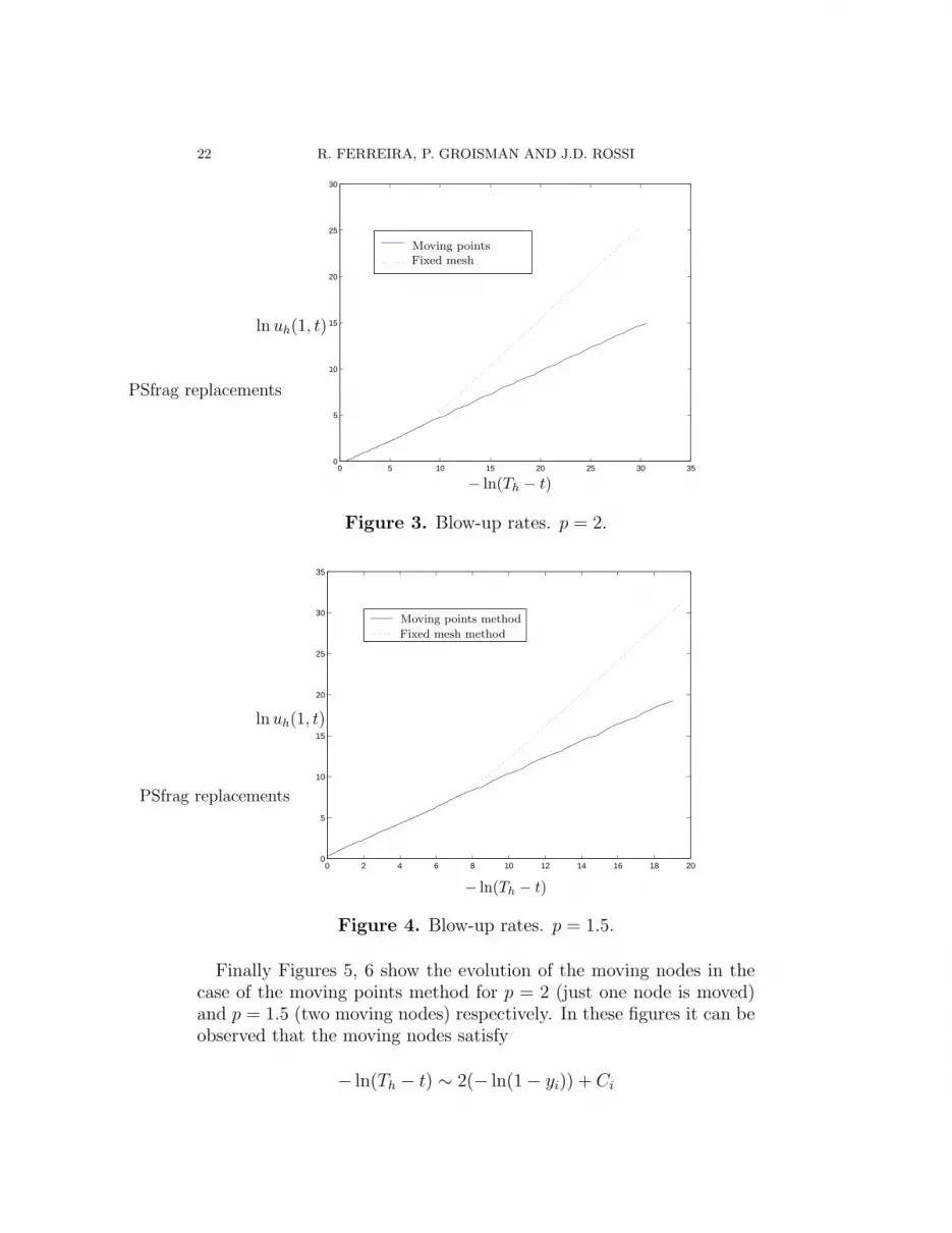
In Figures 3, 4 we show the performance of the moving points method,using the same initial datum and the same powers (p = 2 and p = 1.5)used above. Again we can observe that the slopes of the resulting linesreproduce the expected blow-up rates.


0 5 10 15 20 25 30 350

5

10

15

20

25

30

PSfrag replacements

− ln(Th − t)

ln uh(1, t)

Moving points

Fixed mesh

Figure 3. Blow-up rates. p = 2.

0 2 4 6 8 10 12 14 16 18 200

5

10

15

20

25

30

35

PSfrag replacements

− ln(Th − t)

ln uh(1, t)

Moving points method

Fixed mesh method

Figure 4. Blow-up rates. p = 1.5.

Finally Figures 5, 6 show the evolution of the moving nodes in thecase of the moving points method for p = 2 (just one node is moved)and p = 1.5 (two moving nodes) respectively. In these figures it can beobserved that the moving nodes satisfy

− ln(Th − t) ∼ 2(− ln(1− yi)) + Ci


which means that they obey the scaling invariance of the problem, thatis,

1− yi√Th − t

∼ ξi,

and so this method recovers the self-similar behavior of the continuoussolution as it was proved.

2 4 6 8 10 12 140

5

10

15

20

25

30

35

PSfrag replacements

−ln

(Th−

t)

− ln(1− yK)

Figure 5. Position of the moving point. p = 2.


2 4 6 8 10 12 14−5

0

5

10

15

20

25

30

PSfrag replacements

− ln(1− y1), − ln(1− y2)

−ln

(Th−

t)

y1 y2

Figure 6. Position of the two moving points. p = 1.5.

Comments and Extensions.

Moving mesh methods, based in moving mesh partial differentialequations are also expected to reproduce these asymptotic behaviors,in spite of the evidence is just heuristical and experimental. Rigorousproofs are not available. However, the moving mesh algorithms can beapplied to a large family of problems. The idea behind these proceduresis to take advantage of the self-similar scaling of the problems underconsideration. This seems to us to be the more natural way to faceblow-up problems. Our results can be viewed as a preliminary step toobtain rigorous proofs for these kind of schemes.

The results contained in the paper are restricted to one space dimen-sion. We may try to extend these ideas to several space dimensions. IfΩ is a bounded domain we face the problem ut = ∆u in Ω× (0, T ) witha boundary condition of the form ∂u

∂η= up on ∂Ω× (0, T ) and an initial

datum u0(x). See [13], [17], [21], [28] for references that includes theblow-up rate and set. There is a natural extension of the ideas devel-oped here to deal with the higher dimensional case. However, in orderto extend any of the two adaptive procedures described in Section 2 weneed to have an a priori knowledge of the spatial location of the blow-up set. This is the case for example if the domain under considerationis a square Ω = [0, 1]× [0, 1] for certain initial conditions that forces theblow-up set to be one of the corners (see [19]). Assume that we know


where a single point blow-up set is located and that the maximum ofthe solution is placed at that point for every time (as in the case of thesquare described in [19]), then we place a node at that point and lookfor the asymptotic behavior of that node. It turns out that we get acondition of the form c1 ≤ R(t, hN,1, hN,2, ..., hN,J). When R(t, ·) = c1

we modify the mesh locally near the blow-up point, adding or movingthe adjacent nodes, by performing a contraction by a factor r < 1. Asimple calculation shows that when such a contraction is performed thenew value of R(t, ·) increases, allowing us to proceed just as describedin Section 2.

However, if the maximum of the solution moves from one node toanother then we have to perform adaptive procedures at different pointsthat may compensate as time evolves and hence our proofs are no longervalid.

8. Appendix.

In this appendix we find a supersolution for

Et = Exx + C(T − t)θh (x, t) ∈ (0, 1)× [0, T ),Ex(0, t) = 0 t ∈ [0, T ),Ex(1, t) = C(T − t)−1/2E(1, t) t ∈ [0, T ),E(x, 0) = Ch x ∈ (0, 1),

such that

E(x, t) ≤ Ch(T − t)−γ

and with the first four spatial derivatives positives in [0, 1].Let us look for a supersolution of the form

E(x, t) = Ch(T − t)θa(x, t),

with a(x, t) a solution of

(8.1)

at = axx (x, t) ∈ (0, 1)× [0, T ),ax(0, t) = 0 t ∈ [0, T ),ax(1, t) = C(T − t)−1/2a(1, t) t ∈ [0, T ),a(x, 0) = a0(x) x ∈ (0, 1).

In order to get a supersolution, E, with the first four spatial derivativespositives, we impose that a0(x) is a smooth compatible initial datumwith the first four spatial derivatives positives. The positivity of thederivatives is preserved for every t ∈ [0, T ).

Now let us see that there exists r such that

(8.2) a(x, t) ≤ C

(T − t)r.


To this end we want to construct a supersolution to (8.1) such that (8.2)holds. This can be easily done by the following procedure: take v(x, t)a solution of (1.1) with boundary condition given by vx(1, t) = vq(1, t),with q small, and initial datum v0 such that v(x, t) blows up exactly attime T , see [29] for a proof of the fact that for every time T there existan initial datum such that v(x, t) blows up at time T . The blow-uprate for solutions of (1.1), see [18], [21], gives that v(x, t) verifies

v(1, t) ∼ L

(T − t)1

2(q−1)

,

with Lq−1 → +∞ as q 1, see [18] for an explicit formula for L(q). Letus fix q such that Lq−1(q) > C. With this choice, v is a supersolutionof (8.1). In fact,

vx(1, t) = vq(1, t) = vq−1v(1, t) ≥ Lq−1

(T − t)12

v(1, t),

as we wanted to prove.

Acknowledgements

RF supported by DGES Project PB94-0153, EU Programme TMRFMRX-CT98-0201 and AECI. PG and JDR supported by ANPCyTPICT No. 03-05009, CONICET (Argentina) and AECI. This researchwas finished during a stay of the second and third authors, (PG) and(JDR), at Universidad Autonoma de Madrid. They are grateful to thisinstitution for its hospitality.

We want to thank the referee. His report was a source of inspirationto improve the results of this paper.

References

[1] L. M. Abia, J. C. Lopez-Marcos, J. Martinez. Blow-up for semidiscretizationsof reaction diffusion equations. Appl. Numer. Math. Vol. 20, (1996), 145-156.

[2] L. M. Abia, J. C. Lopez-Marcos, J. Martinez. On the blow-up time convergenceof semidiscretizations of reaction diffusion equations. Appl. Numer. Math.Vol. 26, (1998), 399-414.

[3] G. Acosta, R. Duran and J. D. Rossi. An adaptive time step procedure for aparabolic problem with blow-up. Computing. Vol. 68 (4), (2002), 343-373.

[4] G. Acosta, J. Fernandez Bonder, P. Groisman and J.D. Rossi. Numericalapproximation of a parabolic problem with a nonlinear boundary condition inseveral space dimensions. Discr. Cont. Dyn. Sys. B, Vol. 2 (2), (2002), 279-294.

[5] C. Bandle and H. Brunner. Blow-up in diffusion equations: a survey. J. Comp.Appl. Math. Vol. 97, (1998), 3-22.


[6] C. Bandle and H. Brunner. Numerical analysis of semilinear parabolic prob-lems with blow-up solutions. Rev. Real Acad. Cienc. Exact. Fis. Natur.Madrid. 88, (1994), 203-222.

[7] M. Berger and R. V. Kohn. A rescaling algorithm for the numerical calculationof blowing up solutions. Comm. Pure Appl. Math. Vol. 41, (1988), 841-863.

[8] C. Budd and G. Collins. An invariant moving mesh scheme for the nonlineardiffusion equation. Appl. Numer. Math. Vol. 26, (1998), 23-39.

[9] C. Budd, S. Chen and R. D. Russell. New self-similar solutions of the non-linear Schrodinger equation with moving mesh computations. J. Comp. Phys.Vol. 152, (1999), 756-789.

[10] C. J. Budd, W. Huang and R. D. Russell. Moving mesh methods for problemswith blow-up. SIAM Jour. Sci. Comput. Vol. 17(2), (1996), 305-327.

[11] X. Y. Chen. Asymptotic behaviours of blowing up solutions for finite differenceanalogue of ut = uxx +u1+α. J. Fac. Sci. Univ. Tokyo, Sec IA, Math. Vol. 33,(1986), 541-574.

[12] P. Ciarlet. The finite element method for elliptic problems. North Holland,(1978).

[13] M. Chlebık and M. Fila. On the blow-up rate for the heat equation with anonlinear boundary condition. Math. Methods Appl. Sci., Vol. 23, (2000),1323–1330.

[14] R. G. Duran, J. I. Etcheverry and J. D. Rossi. Numerical approximation of aparabolic problem with a nonlinear boundary condition. Discr. and Cont. Dyn.Sys. Vol. 4 (3), (1998), 497-506.

[15] J. Fernandez Bonder and J. D. Rossi. Blow-up vs. spurious steady solutions.Proc. Amer. Math. Soc. Vol. 129 (1), (2001), 139-144.

[16] R. Ferreira, P. Groisman and J. D. Rossi. Numerical blow-up for a nonlinearproblem with a nonlinear boundary condition. Math. Models Methods Appl.Sci. M3AS. Vol. 12 (4), (2002), 461-484.

[17] M. Fila and J. Filo. Blow-up on the boundary: A survey. Singularities andDifferential Equations, Banach Center Publ., Vol. 33 (S.Janeczko el al., eds.),Polish Academy of Science, Inst. of Math., Warsaw, (1996), pp. 67–78.

[18] M. Fila and P. Quittner. The blowup rate for the heat equation with a nonlinearboundary condition. Math. Methods Appl. Sci., Vol. 14, (1991), 197–205.

[19] M. Fila, J. Filo and G. M. Lieberman. Blow-up on the boundary for the heatequation Calc. Var. Partial Differential Equations, Vol. 10, (2000), 85-99.

[20] W. Huang, Y. Ren and R. D. Russell. Moving mesh partial differential equa-tions (MMPDEs) based on the equidistribution principle. SIAM J. Numer.Anal. Vol 31, (1994), 709-730.

[21] B. Hu and H. M. Yin. The profile near blowup time for solution of theheat equation with a nonlinear boundary condition. Trans. Amer. Math. Soc.,Vol. 346(1), (1994), 117–135.

[22] M. N. Le Roux. Semidiscretizations in time of nonlinear parabolic equationswith blow-up of the solutions. SIAM J. Numer. Anal. Vol. 31, (1994), 170-195.

[23] H. A. Levine. The role of critical exponents in blow up theorems. SIAM Rev.Vol. 32, (1990), 262–288.

[24] H. A. Levine and L. E. Payne. Nonexistence theorems for the heat equationwith nonlinear boundary conditions and for the porous medium equation back-ward in time. J. Differential Equations, Vol. 16, (1974), 319–334.


[25] T. Nakagawa. Blowing up of a finite difference solution to ut = uxx + u2.Appl. Math. Optim., 2, (1976), 337-350.

[26] T. Nakagawa and T. Ushijima. Finite element analysis of the semilinear heatequation of blow-up type. Topics in Numerical Analysis III (J.J.H Miller, ed.),Academic Press, London, (1977), 275-291.

[27] C. V. Pao, “Nonlinear parabolic and elliptic equations”. Plenum Press, NewYork, (1992).

[28] D. F. Rial and J. D. Rossi. Blow-up results and localization of blow-up pointsin an N−dimensional smooth domain. Duke Math. J., Vol. 88(2), (1997),391–405.

[29] J. D. Rossi. The blow-up rate for a system of heat equations with nontrivialcoupling at the boundary. Math. Methods Appl. Sci., vol 20, (1997), 1-11.

[30] A. A. Samarskii, V. A. Galaktionov, S. P. Kurdyumov and A. P. Mikhailov.“Blow-up in problems for quasilinear parabolic equations”. Nauka, Moscow,(1987) (in Russian). English transl.: Walter de Gruyter, Berlin, (1995).

[31] W. Walter. On existence and nonexistence in the large of solutions of parabolicdifferential equations with a nonlinear boundary condition. SIAM J. Math.Anal., Vol. 6(1), (1975), 85–90.

Depto. de Matematicas, U. Autonoma de Madrid, 28049 Madrid,Spain.

E-mail address: [email protected]

Universidad de San Andres, Vito Dumas 284 (1644) Victoria, Pcia.de Buenos Aires, Argentina


Depto. de Matematica, FCEyN., UBA, (1428) Buenos Aires, Ar-gentina.


Documents

Adaptive numerical schemes for a parabolic problem with blow-up