Embed Size (px)
Citation preview
Li, H, Liu, J, Yang, Z, Liu, RW, Wu, K and Wan, Y
Adaptively constrained dynamic time warping for time series classification and clustering
http://researchonline.ljmu.ac.uk/id/eprint/13159/
Article
LJMU has developed LJMU Research Online for users to access the research output of the University more effectively. Copyright © and Moral Rights for the papers on this site are retained by the individual authors and/or other copyright owners. Users may download and/or print one copy of any article(s) in LJMU Research Online to facilitate their private study or for non-commercial research.You may not engage in further distribution of the material or use it for any profit-making activities or any commercial gain.
The version presented here may differ from the published version or from the version of the record. Please see the repository URL above for details on accessing the published version and note that access may require a subscription.
For more information please contact [email protected]
http://researchonline.ljmu.ac.uk/
Citation (please note it is advisable to refer to the publisher’s version if you intend to cite from this work)
Li, H, Liu, J, Yang, Z, Liu, RW, Wu, K and Wan, Y (2020) Adaptively constrained dynamic time warping for time series classification and clustering. Information Sciences, 534. pp. 97-116. ISSN 0020-0255
LJMU Research Online
Adaptively constrained dynamic time warping for time series classification
and clustering
Huanhuan Li a,b,c, Jingxian Liu a,b, Zaili Yang c*, Ryan Wen Liu a,b*, Kefeng Wu d, Yuan Wan e
a Hubei Key Laboratory of Inland Shipping Technology, School of Navigation, Wuhan University of Technology, Wuhan 430063, P. R. China b National Engineering Research Center for Water Transport Safety, Wuhan 430063, P. R. China c Liverpool Logistics, Offshore and Marine Research Institute, Liverpool John Moores University, Liverpool L3 3AF, UK d Beijing Electro-mechanical Engineering Institute, Beijing 100074, P. R. China e School of Science, Wuhan University of Technology, Wuhan 430070, P. R. China
*Corresponding author.
E-mail address: [email protected]; [email protected].
Abstract: Time series classification and clustering are important for data mining research, which is
conducive to recognizing movement patterns, finding customary routes, and detecting abnormal
trajectories in transport (e.g. road and maritime) traffic. The dynamic time warping (DTW)
algorithm is a classical distance measurement method for time series analysis. However, the over-
stretching and over-compression problems are typical drawbacks of using DTW to measure
distances. To address these drawbacks, an adaptive constrained DTW (ACDTW) algorithm is
developed to calculate the distances between trajectories more accurately by introducing new
adaptive penalty functions. Two different penalties are proposed to effectively and automatically
adapt to the situations in which multiple points in one time series correspond to a single point in
another time series. The novel ACDTW algorithm can adaptively adjust the correspondence between
two trajectories and obtain greater accuracy between different trajectories. Numerous experiments
on classification and clustering are undertaken using the UCR time series archive and real vessel
trajectories. The classification results demonstrate that the ACDTW algorithm performs better than
four state-of-the-art algorithms on the UCR time series archive. Furthermore, the clustering results
reveal that the ACDTW algorithm has the best performance among three existing algorithms in
modeling maritime traffic vessel trajectory.
Keywords: Dynamic time warping, Distance measure, Time series classification, Vessel trajectory
clustering.
1. Introduction
1.1 Background and related work
With the explosion of the Internet of Things (IoT), sensor networks and radar systems, a large
number of time series are continuously produced in various fields, such as intelligent transportation,
maritime engineering, clinical medicine, biological science, climate research, and social science [20,
44]. Different types of time series have been created and applied in the studies relating to hurricanes,
animals, people, vessels, vehicles, and speech signals, etc [37]. Time series data mining can uncover
hidden patterns and extract behavior characteristics. Time series classification and clustering are
important for data mining of moving object trajectories [1, 50].
As an important kind of complex data, the time series of moving vessels play an indispensable
role in maritime traffic networks, surveillance, and security research fields [22]. In the maritime
traffic domain, the results of time series classification and clustering are conducive to investigating
path planning[25], abnormal detection [7], and movement pattern recognition [38]. The automatic
identification system (AIS) provides real-time spatiotemporal information of vessels, including time,
position, speed over ground, course over ground, and rate of turn, etc. AIS is complementary to
radar systems, and the temporal resolution of the AIS signal is commonly enhanced through marine
radar by data fusion technology, allowing vessel trajectories to be tagged with useful information [45]. AIS systems have been widely used on vessels to identify targets and enhance maritime
surveillance based on a very high frequency (VHF) data communication scheme, especially for large
cooperating vessels [2]. Trajectory classification aims at identifying features and patterns by
analyzing the objects’ movement awareness and other spatiotemporal information in a time series
[31]. AIS-based vessel trajectory clustering is of significance in mining customary routes,
identifying abnormal patterns, improving navigational safety, and safeguarding maritime
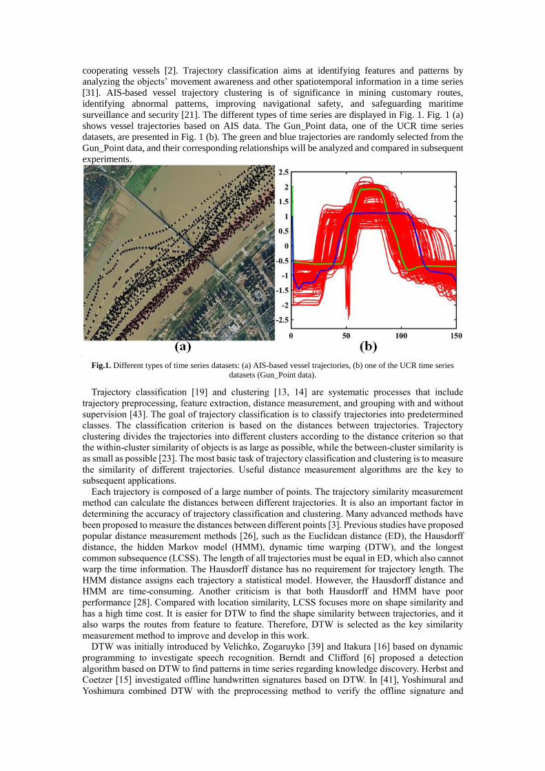
surveillance and security [21]. The different types of time series are displayed in Fig. 1. Fig. 1 (a)
shows vessel trajectories based on AIS data. The Gun_Point data, one of the UCR time series
datasets, are presented in Fig. 1 (b). The green and blue trajectories are randomly selected from the
Gun_Point data, and their corresponding relationships will be analyzed and compared in subsequent
experiments.
Fig.1. Different types of time series datasets: (a) AIS-based vessel trajectories, (b) one of the UCR time series
datasets (Gun_Point data).
Trajectory classification [19] and clustering [13, 14] are systematic processes that include
trajectory preprocessing, feature extraction, distance measurement, and grouping with and without
supervision [43]. The goal of trajectory classification is to classify trajectories into predetermined
classes. The classification criterion is based on the distances between trajectories. Trajectory
clustering divides the trajectories into different clusters according to the distance criterion so that
the within-cluster similarity of objects is as large as possible, while the between-cluster similarity is
as small as possible [23]. The most basic task of trajectory classification and clustering is to measure
the similarity of different trajectories. Useful distance measurement algorithms are the key to
subsequent applications.
Each trajectory is composed of a large number of points. The trajectory similarity measurement
method can calculate the distances between different trajectories. It is also an important factor in
determining the accuracy of trajectory classification and clustering. Many advanced methods have
been proposed to measure the distances between different points [3]. Previous studies have proposed
popular distance measurement methods [26], such as the Euclidean distance (ED), the Hausdorff
distance, the hidden Markov model (HMM), dynamic time warping (DTW), and the longest
common subsequence (LCSS). The length of all trajectories must be equal in ED, which also cannot
warp the time information. The Hausdorff distance has no requirement for trajectory length. The
HMM distance assigns each trajectory a statistical model. However, the Hausdorff distance and
HMM are time-consuming. Another criticism is that both Hausdorff and HMM have poor
performance [28]. Compared with location similarity, LCSS focuses more on shape similarity and
has a high time cost. It is easier for DTW to find the shape similarity between trajectories, and it
also warps the routes from feature to feature. Therefore, DTW is selected as the key similarity
measurement method to improve and develop in this work.
DTW was initially introduced by Velichko, Zogaruyko [39] and Itakura [16] based on dynamic
programming to investigate speech recognition. Berndt and Clifford [6] proposed a detection
algorithm based on DTW to find patterns in time series regarding knowledge discovery. Herbst and Coetzer [15] investigated offline handwritten signatures based on DTW. In [41], Yoshimural and
Yoshimura combined DTW with the preprocessing method to verify the offline signature and
identify suspect signatures. In [34], Shanker and Rajagopalan proposed the DTW-based method to
construct an effective offline signature verification system. The code-vectors and DTW are merged
into the online signature verification strategy in [35] to improve the accuracy of the system. In [25],
Liu et al. measured the similarity between trajectories and calculated the distance based on DTW to
cluster the vessel trajectories and mine customary routes. In [21], Li et al. considered the distances
between trajectories based on DTW and proposed the multistep clustering method to cluster vessel
trajectories and detect abnormal trajectories. In [48], Zhao et al. combined DTW and the trajectory
shape to analyze the distances between trajectories and mine trajectory movement patterns.
These studies have shown that DTW is a kind of nonlinear programming technique based on time
programming and distance testing [30]. It can be used to calculate the similarity between two time
series and eventually find the shortest distance [9]. DTW can find the optimal path with a minimum
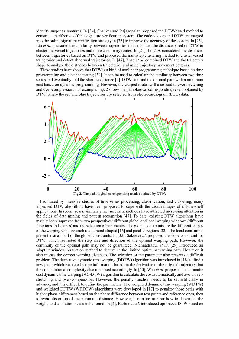
cost based on dynamic programming. However, the warped routes will also lead to over-stretching
and over-compression. For example, Fig. 2 shows the pathological corresponding result obtained by
DTW, where the red and blue trajectories are selected from electrocardiogram (ECG) data.
Fig.2. The pathological corresponding result obtained by DTW.
Facilitated by intensive studies of time series processing, classification, and clustering, many
improved DTW algorithms have been proposed to cope with the disadvantages of off-the-shelf
applications. In recent years, similarity measurement methods have attracted increasing attention in
the fields of data mining and pattern recognition [47]. To date, existing DTW algorithms have
mainly been improved from two perspectives: different global and local warping windows (different
functions and shapes) and the selection of parameters. The global constraints are the different shapes
of the warping window, such as diamond-shaped [16] and parallel regions [32]. The local constraints
present a small part of the global constraints. In [32], Sakoe et al. proposed the slope constraint for
DTW, which restricted the step size and direction of the optimal warping path. However, the
continuity of the optimal path may not be guaranteed. Niennattrakul et al. [29] introduced an
adaptive window restriction method to determine the limited optimum warping path. However, it
also misses the correct warping distances. The selection of the parameter also presents a difficult
problem. The derivative dynamic time warping (DDTW) algorithm was introduced in [18] to find a
new path, which extracted shape information based on the derivative of the original trajectory, but
the computational complexity also increased accordingly. In [40], Wan et al. proposed an automatic
cost dynamic time warping (AC-DTW) algorithm to calculate the cost automatically and avoid over-
stretching and over-compression. However, the penalty function needs to be set artificially in
advance, and it is difficult to define the parameters. The weighted dynamic time warping (WDTW)
and weighted DDTW (WDDTW) algorithms were developed in [17] to penalize those paths with
higher phase differences based on the phase difference between test points and reference ones, then to avoid distortion of the minimum distance. However, it remains unclear how to determine the
weight, and a solution needs to be found. In [4], Barbon et al. introduced optimized DTW based on
the discrete wavelet transform (DWT) to handle long single sequences and avoid the high
computational cost. Fast dynamic time warping (FastDTW), an approximate DTW, was introduced
in [33], which refined the optimal results based on a multilevel approach with linear time and space
complexity. A novel time alignment measurement was proposed in [11], which could better
characterize the signals. The temporal similarity information was extracted by comparing fractions
of the time distortion. Novel elastic distances were proposed to further measure the amplitude
difference in [24]. In [27], Morel et al. introduced a new tolerance to the calculation process and
extended the measurement to an area of more than two time series based on DTW barycenter
averaging (DBA) and constrained dynamic time warping (CDTW). In [48], Zhao et al. considered
the combination of shape and character in the local trajectory to calculate the distance based on the
original DTW and the compensation coefficient. However, the proposed method does not
fundamentally improve the DTW algorithm, and different vessel trajectory characteristics cannot be
measured uniformly. In [49], Zhao et al. developed the DTW method based on Douglas-Peucker
compression and conducted clustering analysis based on the improved density-based spatial
clustering of applications with noise (DBSCAN). However, this improvement cannot reduce some
points based on the compression algorithm unless the algorithm is changed or the many-to-one and
one-to-many problems are solved.
1.2 Motivation and contribution
The traditional DTW algorithm [6, 15, 34, 41, 42, 46] usually ignores extreme cases such as many-
to-one and one-to-many when the numbers of points in different time series are extremely different.
It also ignores the number of times that each point is used in the time series similarity measurement.
Additionally, it does not take into account the fact that the number of points between two trajectories
can vary significantly in different application aspects. Many improved DTW algorithms [4, 27, 29,
32, 40, 48] lack a unified standard and solution for the warping window shape, weight, and step size.
In addition, some improved DTW algorithms also require manually preselected parameters.
Extreme cases still exist in many improved DTW algorithms. To facilitate comparison with other
algorithms, all the improved DTW algorithms are validated on the widely-used UCR time series
with equal length. However, the pathological matching of time series is generally not considered in
the mentioned warping algorithms. To address the potential limitations in traditional DTW
algorithms, this paper proposes an adaptive constrained dynamic time warping (ACDTW) algorithm
by considering adaptive penalty functions. In particular, ACDTW has the capacity to alleviate
pathological matching and increase the accuracy of similarity measurement. Furthermore, it is not
necessary to consider the window size and preselect the manual parameters for ACDTW in practical
applications. Two kinds of adaptive penalty functions for time series are proposed in ACDTW: one
for time series with equal length and the other for time series with unequal length. Each kind of
adaptive penalty function consists of two parts: the length of the trajectory and the number of times
that each point in the time series is used in each step. The proposed ACDTW can automatically
adjust the correspondence of the time series, select the optimal matching, and increase the accuracy
of the similarity measurement between different time series.
Given the state-of-the-art studies, the major contributions presented in this work are summarized
as follows:
• To effectively handle extreme cases, the ACDTW algorithm is proposed to accurately calculate
the distances between different time series. It can essentially reduce over-stretching and over-
compression while improving the accuracy of distance calculation.
• The adaptive penalty functions can automatically adjust the correspondence of the time series
and warp the optimal matching in each step of ACDTW. They can reduce the distance between time
series with high similarity and increase the accuracy of subsequent experiments.
• Comprehensive experiments have been implemented on the UCR time series archive with equal
length and realistic vessel trajectory dataset with unequal length. The results of time series
classification and clustering have demonstrated the effectiveness of our ACDTW.
Automatic and valid penalty functions in the warping process can help make adjustments and find
the optimal path. In this paper, the ACDTW algorithm is proposed to calculate accurate distances
and reduce over-stretching and over-compression based on the penalty function of each point. The greater the similarity between two time series, the smaller the distance. ACDTW can reduce the
distance between time series with high similarity while increasing the distance between time series
with low similarity. The novel penalty function can set the weight of each step automatically to
select the optimal warping path. Based on the automatic warping of the novel penalty function,
ACDTW can avoid many-to-one and one-to-many matching when calculating the distance and
finding the optimal path between two trajectories. It enables an improvement in the accuracy of
measuring trajectory distances, which can help preserve effective features, mine trajectory patterns,
and support decision making effectively through trajectory classification and clustering.
The remainder of this paper is organized as follows. Section 2 briefly reviews the original DTW
algorithm. In Section 3, the ACDTW algorithm is proposed and described systematically to analyze
time series. In Section 4, numerous experiments are conducted based on 22 datasets from the UCR
time series archive and a vessel trajectory dataset by classification and clustering respectively, to
demonstrate the effectiveness of our method in practical applications. Finally, Section 5 concludes
this paper by summarizing its novel contributions and future research directions.
2. A brief review of DTW
From a statistical point of view, a spatiotemporal AIS trajectory is essentially a kind of time series.
Suppose 1 2={ , , , }mQ q q q and
1 2={ , , , }nC c c c denote two AIS trajectories (i.e., time series),
iq represents the value of the ith point in series Q , jc indicates the value of the jth point in series
C , m and n represent the length of the two sequences, respectively. ,i jd q c denotes the
distance between iq and , 2,3, , , 2,3,jc i m j n .
DTW is used to calculate the maximum similarity between the two time series [12]. The principle
of DTW is as follows:
Allocate all points in sequence according to time and then construct the matrix m nA , in which
2( , ) ( )ij i j i j m na d q c q c A . A set of adjacent matrix elements in m nA is called the
warping path, denoted by 1 2, , , , ,t KW w w w w ; max , 1m n K m n , and the tht
point in W is represented by t ij tw a .
The warping path must satisfy the following constraints:
(1) Boundary condition: 1 11, ;K mnw a w a
(2) Continuity and monotonicity: if -1 ,t i j t ijw a w a , then ' '0 1, 0 1i i j j ,which
ensures that every coordinate in the two trajectories can appear in W, and the corresponding of points
between the trajectories does not intersect. The time at each point is also monotonic in W.
Specifically, DTW can be calculated as follows:
1
( , )
( , ) min{ / }
t i j
K
t t
w d q c
DTW Q C w K
(1)
where tw is the distance between the corresponding points iq and jc in the two series, and K
is the length of the longer sequence.
The steps involved in the algorithm are as follows [36]:
Step 1. Calculate the DTW distance ( , )D i j between the two sequences from the starting points
andi j of the two sequences.
11
2
(1,1)
( , ) min ( 1, 1), ( , 1), ( 1, )
( , ) ( )
ij
ij i j i j m n
D d
D i j d D i j D i j D i j
d d q c q c D
(2)
Step 2. The distance ( , )D i j of the endpoint in the two sequences is the DTW distance of the
two sequences.
The pseudocode of the DTW algorithm is as follows.
Algorithm 1: DTW algorithm
Input: 1 2={ , , , }mQ q q q and
1 2={ , , , }nC c c c // the two time series
Output: The optimal warping path;
The distance of Q and C .
Initialize: 1,1(1,1)DTW d
for i=1:n
for j=1:m
,1 ( 1, )i jD d DTW i j
,2 ( 1, 1)i jD d DTW i j
,3 ( , 1)i jD d DTW i j
min( 1, 2, 3)DTW D D D ;
The optimal pathi,j =min_index((i-1, j), (i-1, j-1), (i, j-1))
end
end
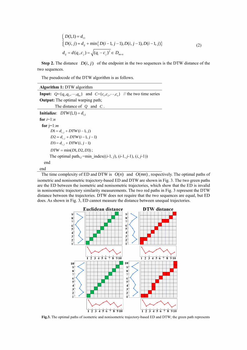
The time complexity of ED and DTW is ( )O n and ( )O mn , respectively. The optimal paths of
isometric and nonisometric trajectory-based ED and DTW are shown in Fig. 3. The two green paths
are the ED between the isometric and nonisometric trajectories, which show that the ED is invalid
in nonisometric trajectory similarity measurements. The two red paths in Fig. 3 represent the DTW
distance between the trajectories. DTW does not require that the two sequences are equal, but ED
does. As shown in Fig. 3, ED cannot measure the distance between unequal trajectories.
Fig.3. The optimal paths of isometric and nonisometric trajectory-based ED and DTW; the green path represents
Euclidean distance, and the red warping path expresses DTW distance.
3. The Proposed ACDTW algorithm
Penalty functions and ACDTW are introduced in this paper to reduce many-to-one and one-to-
many matching. ACDTW comprehensively takes into account the use of each point, and the more
times each point is used, the greater the penalty function value. The optimal warping path is selected
based on the adaptive penalty functions and the number of times each point is used in each step.
3.1 The adaptive penalty functions
3.1.1 The adaptive penalty function for time series with equal length
The adaptive penalty function for time series with equal length takes into account the number of
times each point is used in each step as well as the trajectories lengths. It is proposed based on the
point mean idea, which does not restrict the trajectory length, as described in Eq. (3):
, , ,( ) [( ) / max( , )] ( ) ( )2 2max( , )
2, , ; , 2, , .
i j i j i j
m n m nc x m n N x N x
m n
i m j n
(3)
where ,( )i jN x denotes how many times each point is used in the matching process. m and n
are the length of two trajectories. 2max( , )
m n
m n
is constant when m and n are defined, and it is
used to numerically control the tolerance of many-to-one and one-to-many matching.
It is easy to deduce that min( , )1( )
max( , ) 2max( , )
m n m nm n
m n m n
, so
2max( , )
m n
m n
will increase
when m and n become closer. Then, ,( )i jc x is positively proportional to ,( )i jN x , meaning
that when ,( )i jN x increases, ,( )i jc x increases simultaneously. A higher value of 2max( , )
m n
m n
amplifies the unacceptable degree of many-to-one and one-to-many matching, while a lower value
diminishes this effect.
The value of the penalty function increases with the proximity of the two time series. This means
that the closer the lengths of two time series are, the lower the tolerance of many-to-one and one-
to-many matching.
3.1.2 The adaptive penalty function for time series with unequal length
The adaptive penalty function for time series with unequal length takes into account the effects
of different trajectory lengths. It is enhanced based on the point mean and dual restriction ideas, as
follows:
,
,
,
,
,
1 1[( ) / max( , )] ( ), 0 0
2 2 2( )
1 1[max( , ) / ( )] ( ),
2 2 2
1 1( ), 0 0
2max( , ) 2 2
2max( , ) 1 1( ),
2 2
i j
i j
i j
i j
i j
m n m nm n N x or
n mc x
m n m nm n N x or
n m
m n m nN x or
m n n m
m n m nN x or
m n n m
(4)
This penalty function considers the trajectory length and limits cases where the trajectory is closer
or farther. 2max( , )m n
m n and
2max( , )
m n
m n
are constant when m and n are defined, and they
are used to numerically control the tolerance of many-to-one and one-to-many as m and n
become closer or farther.
It is easy to show that min( , ) 2max( , )1( ) 2
max( , ) 2max( , )
m n m n m nm n
m n m n m n
, so
2max( , )
m n
m n
will become larger as m and n become closer, and 2max( , )m n
m n will become
larger as m and n move farther apart. A higher value of the penalty function amplifies the
unacceptable degree of many-to-one and one-to-many matching.
The value of the penalty function increases with the proximity and the separation of two time
series, indicating that the closer or farther the two time series are, the lower the tolerance of many-
to-one and one-to-many matching.
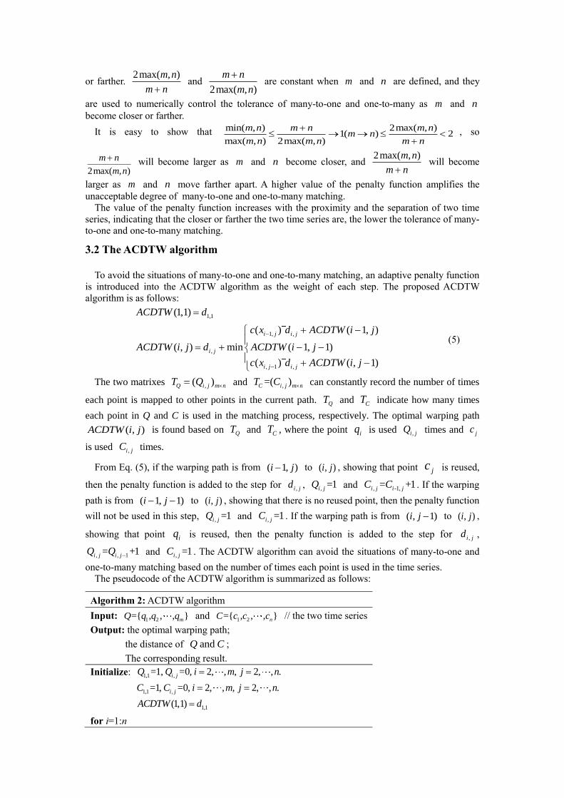
3.2 The ACDTW algorithm
To avoid the situations of many-to-one and one-to-many matching, an adaptive penalty function
is introduced into the ACDTW algorithm as the weight of each step. The proposed ACDTW
algorithm is as follows:
1,1
1, ,
,
, 1 ,
(1,1)
( ) ( 1, )
( , ) min ( 1, 1)
( ) ( , 1)
i j i j
i j
i j i j
ACDTW d
c x d ACDTW i j
ACDTW i j d ACDTW i j
c x d ACDTW i j
(5)
The two matrixes ,( )Q i j m nT Q and ,=( )C i j m nT C can constantly record the number of times
each point is mapped to other points in the current path. QT and CT indicate how many times
each point in Q and C is used in the matching process, respectively. The optimal warping path
( , )ACDTW i j is found based on QT and CT , where the point iq is used ,i jQ times and jc
is used ,i jC times.
From Eq. (5), if the warping path is from ( 1, )i j to ( , )i j , showing that point jc is reused,
then the penalty function is added to the step for ,i jd , , =1i jQ and , -1,= +1i j i jC C . If the warping
path is from ( 1, 1)i j to ( , )i j , showing that there is no reused point, then the penalty function
will not be used in this step, , =1i jQ and , =1i jC . If the warping path is from ( , 1)i j to ( , )i j ,
showing that point iq is reused, then the penalty function is added to the step for ,i jd ,
, , 1= +1i j i jQ Q and , =1i jC . The ACDTW algorithm can avoid the situations of many-to-one and
one-to-many matching based on the number of times each point is used in the time series.
The pseudocode of the ACDTW algorithm is summarized as follows:
Algorithm 2: ACDTW algorithm
Input: 1 2={ , , , }mQ q q q and
1 2={ , , , }nC c c c // the two time series
Output: the optimal warping path;
the distance of andQ C ;
The corresponding result.
Initialize: 1,1 ,=1, =0, 2, , , 2, , .i jQ Q i m j n
1,1 ,=1, =0, 2, , , 2, , .i jC C i m j n
1,1(1,1)ACDTW d
for i=1:n
for j=1:m
, 1, ,1 ( ) ( 1, )i j i j i jD d c x d ACDTW i j
,2 ( 1, 1)i jD d ACDTW i j
, , 1 ,3 ( ) ( , 1)i j i j i jD d c x d ACDTW i j
( , ) min( 1, 2, 3)ACDTW i j D D D ;
The optimal pathi,j =min_index((i-1, j), (i-1, j-1), (i, j-1))
if ( , ) 1ACDTW i j D
then , , -1,=1 = +1i j i j i jQ C C, ;
else if ( , ) 2ACDTW i j D
then , ,=1 =1i j i jQ C, ;
else ( , ) 3ACDTW i j D
then , , 1 ,= +1 =1i j i j i jQ Q C , .
Result = D (m, n)
end
end
end
4. Experimental results and analysis
DTW and its variants are proposed for matching similar time series and measuring the distances
between time series. In the first classification experiment, we evaluate the classification
performance of five state-of-the-art methods and demonstrate the validity of ACDTW as a distance
measure on 22 benchmark datasets by the nearest neighbor classification. In the second clustering
experiment, the performance of three distance measurement methods is provided and compared to
further verify the accuracy and effectiveness of ACDTW on a real vessel trajectory dataset.
Descriptions of the datasets, experimental setup, and performance analysis for classification and
clustering are given in the following sections.
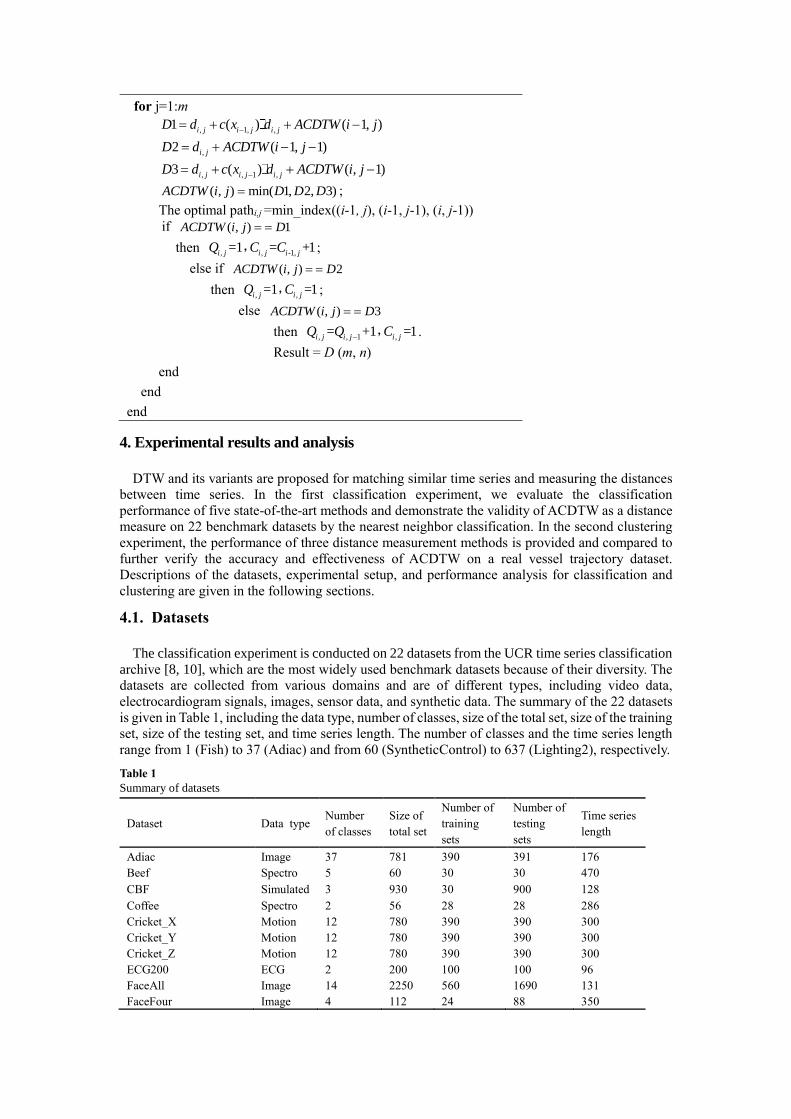
4.1. Datasets
The classification experiment is conducted on 22 datasets from the UCR time series classification
archive [8, 10], which are the most widely used benchmark datasets because of their diversity. The
datasets are collected from various domains and are of different types, including video data,
electrocardiogram signals, images, sensor data, and synthetic data. The summary of the 22 datasets
is given in Table 1, including the data type, number of classes, size of the total set, size of the training
set, size of the testing set, and time series length. The number of classes and the time series length
range from 1 (Fish) to 37 (Adiac) and from 60 (SyntheticControl) to 637 (Lighting2), respectively.
Table 1
Summary of datasets
Dataset Data type Number
of classes
Size of
total set
Number of
training
sets
Number of
testing
sets
Time series
length
Adiac Image 37 781 390 391 176
Beef Spectro 5 60 30 30 470
CBF Simulated 3 930 30 900 128
Coffee Spectro 2 56 28 28 286
Cricket_X Motion 12 780 390 390 300
Cricket_Y Motion 12 780 390 390 300
Cricket_Z Motion 12 780 390 390 300
ECG200 ECG 2 200 100 100 96
FaceAll Image 14 2250 560 1690 131
FaceFour Image 4 112 24 88 350
Fish Image 1 350 175 175 463
Gun_Point Motion 2 200 50 150 150
LargeKitchenAppliances Device 3 750 375 375 720
Lighting2 Sensor 2 121 60 61 637
OliveOil Spectro 4 60 30 30 570
OSULeaf Image 6 442 200 242 427
ShapeletSim Simulated 2 200 20 180 500
SmallKitchenAppliances Device 3 750 375 375 720
Symbols Image 6 1000 25 995 398
SyntheticControl Simulated 6 600 300 300 60
Trace Sensor 4 200 100 100 275
TwoLeadECG ECG 2 1162 23 1139 82
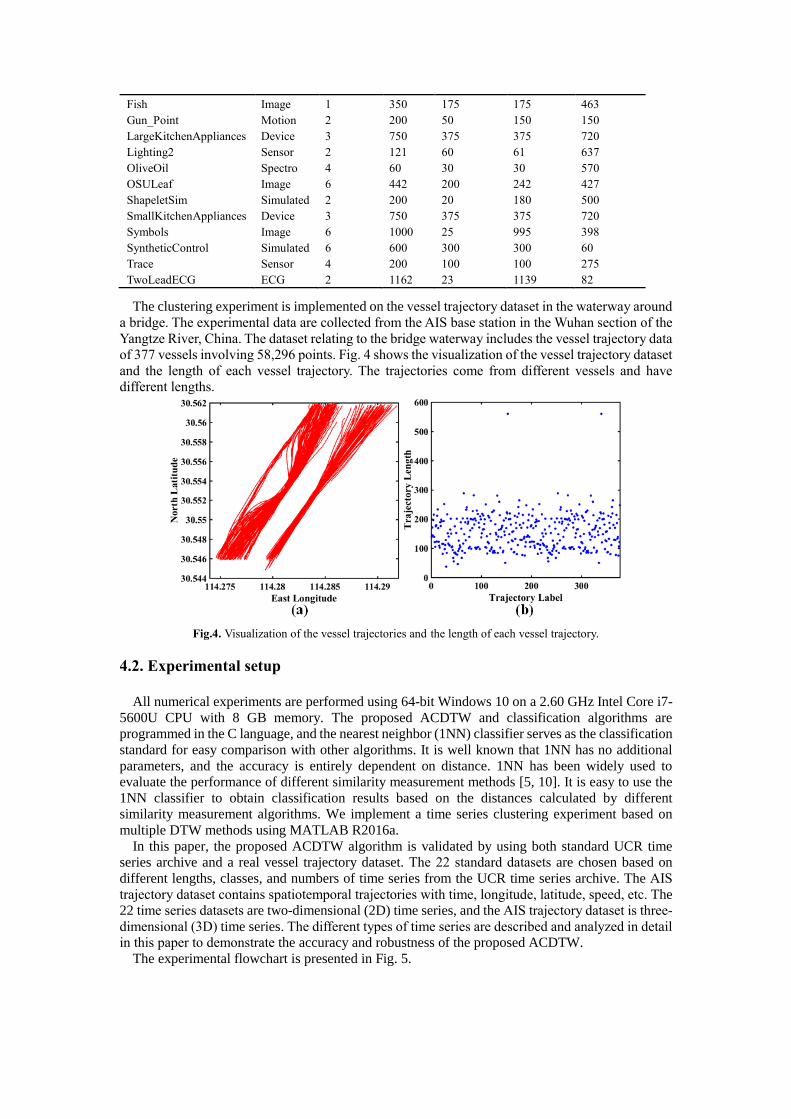
The clustering experiment is implemented on the vessel trajectory dataset in the waterway around
a bridge. The experimental data are collected from the AIS base station in the Wuhan section of the
Yangtze River, China. The dataset relating to the bridge waterway includes the vessel trajectory data
of 377 vessels involving 58,296 points. Fig. 4 shows the visualization of the vessel trajectory dataset
and the length of each vessel trajectory. The trajectories come from different vessels and have
different lengths.
Fig.4. Visualization of the vessel trajectories and the length of each vessel trajectory.
4.2. Experimental setup
All numerical experiments are performed using 64-bit Windows 10 on a 2.60 GHz Intel Core i7-
5600U CPU with 8 GB memory. The proposed ACDTW and classification algorithms are
programmed in the C language, and the nearest neighbor (1NN) classifier serves as the classification
standard for easy comparison with other algorithms. It is well known that 1NN has no additional
parameters, and the accuracy is entirely dependent on distance. 1NN has been widely used to
evaluate the performance of different similarity measurement methods [5, 10]. It is easy to use the
1NN classifier to obtain classification results based on the distances calculated by different
similarity measurement algorithms. We implement a time series clustering experiment based on
multiple DTW methods using MATLAB R2016a.
In this paper, the proposed ACDTW algorithm is validated by using both standard UCR time
series archive and a real vessel trajectory dataset. The 22 standard datasets are chosen based on
different lengths, classes, and numbers of time series from the UCR time series archive. The AIS
trajectory dataset contains spatiotemporal trajectories with time, longitude, latitude, speed, etc. The
22 time series datasets are two-dimensional (2D) time series, and the AIS trajectory dataset is three-
dimensional (3D) time series. The different types of time series are described and analyzed in detail
in this paper to demonstrate the accuracy and robustness of the proposed ACDTW.
The experimental flowchart is presented in Fig. 5.
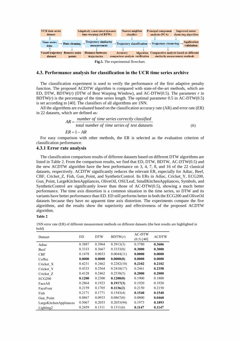
Fig.5. The experimental flowchart.
4.3. Performance analysis for classification in the UCR time series archive
The classification experiment is used to verify the performance of the first adaptive penalty
function. The proposed ACDTW algorithm is compared with state-of-the-art methods, which are
ED, DTW, BDTW(r) (DTW of Best Warping Window), and AC-DTW(0.5). The parameter r in
BDTW(r) is the percentage of the time series length. The optimal parameter 0.5 in AC-DTW(0.5)
is set according to [40]. The classifiers of all algorithms are 1NN.
All the algorithms are evaluated based on the classification accuracy rate (AR) and error rate (ER)
in 22 datasets, which are defined as:
1
number of time series correctly classifiedAR
total number of time series of test datasets
ER AR
(6)
For easy comparison with other methods, the ER is selected as the evaluation criterion of
classification performance.
4.3.1 Error rate analysis
The classification comparison results of different datasets based on different DTW algorithms are
listed in Table 2. From the comparison results, we find that ED, DTW, BDTW, AC-DTW(0.5) and
the new ACDTW algorithm have the best performance on 3, 4, 7, 8, and 16 of the 22 classical
datasets, respectively. ACDTW significantly reduces the relevant ER, especially for Adiac, Beef,
CBF, Cricket_Z, Fish, Gun_Point, and SyntheticControl. Its ERs in Adiac, Cricket_Y, ECG200,
Gun_Point, LargeKitchenAppliances, OliveOil, OSULeaf, SmallKitchenAppliances, Symbols, and
SyntheticControl are significantly lower than those of AC-DTW(0.5), showing a much better
performance. The time axis distortion is a common situation in the time series, so DTW and its
variants have better performance than ED. ED still performs better in both the ECG200 and OliveOil
datasets because they have no apparent time axis distortion. The experiments compare the five
algorithms, and the results show the superiority and effectiveness of the proposed ACDTW
algorithm.
Table 2
1NN error rate (ER) of different measurement methods on different datasets (the best results are highlighted in
bold)
Dataset ED DTW BDTW(r) AC-DTW
(0.5) [40] ACDTW
Adiac 0.3887 0.3964 0.3913(3) 0.3780 0.3606
Beef 0.3333 0.3667 0.3333(0) 0.3000 0.3000
CBF 0.1478 0.0033 0.0044(11) 0.0000 0.0000
Coffee 0.0000 0.0000 0.0000(0) 0.0000 0.0000
Cricket_X 0.4231 0.2462 0.2282(10) 0.2102 0.2102
Cricket_Y 0.4333 0.2564 0.2410(17) 0.2461 0.2358
Cricket_Z 0.4128 0.2462 0.2538(5) 0.2000 0.2000
ECG200 0.1200 0.2300 0.1200(0) 0.1900 0.1800
FaceAll 0.2864 0.1923 0.1917(3) 0.1920 0.1920
FaceFour 0.2159 0.1705 0.1136(2) 0.2150 0.2150
Fish 0.2171 0.1771 0.1543(4) 0.1540 0.1540
Gun_Point 0.0867 0.0933 0.0867(0) 0.0800 0.0460
LargeKitchenAppliances 0.5067 0.2053 0.2053(94) 0.1973 0.1893
Lighting2 0.2459 0.1311 0.1311(6) 0.1147 0.1147
OliveOil 0.1333 0.1667 0.1333(0) 0.1667 0.1333
OSULeaf 0.4793 0.4091 0.3884(7) 0.3884 0.3842
ShapeletSim 0.4611 0.3500 0.3000(3) 0.3278 0.3333
SmallKitchenAppliances 0.6587 0.3573 0.3280(15) 0.3573 0.3413
Symbols 0.1005 0.0503 0.0623(8) 0.0430 0.0400
SyntheticControl 0.1200 0.0067 0.0167(6) 0.0100 0.0067
Trace 0.2400 0.0000 0.0100(3) 0.0000 0.0000
TwoLeadECG 0.2529 0.0957 0.1317(4) 0.1281 0.1281
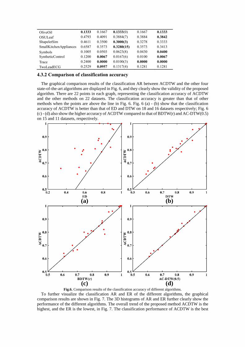
4.3.2 Comparison of classification accuracy
The graphical comparison results of the classification AR between ACDTW and the other four
state-of-the-art algorithms are displayed in Fig. 6, and they clearly show the validity of the proposed
algorithm. There are 22 points in each graph, representing the classification accuracy of ACDTW
and the other methods on 22 datasets. The classification accuracy is greater than that of other
methods when the points are above the line in Fig. 6. Fig. 6 (a) - (b) show that the classification
accuracy of ACDTW is better than that of ED and DTW on 18 and 16 datasets respectively; Fig. 6
(c) - (d) also show the higher accuracy of ACDTW compared to that of BDTW(r) and AC-DTW(0.5)
on 15 and 11 datasets, respectively.
(d)
(b)
(c)
(a)
Fig.6. Comparison results of the classification accuracy of different algorithms. To further visualize the classification AR and ER of the different algorithms, the graphical
comparison results are shown in Fig. 7. The 3D histograms of AR and ER further clearly show the
performance of the different algorithms. The overall trend of the proposed method ACDTW is the highest, and the ER is the lowest, in Fig. 7. The classification performance of ACDTW is the best
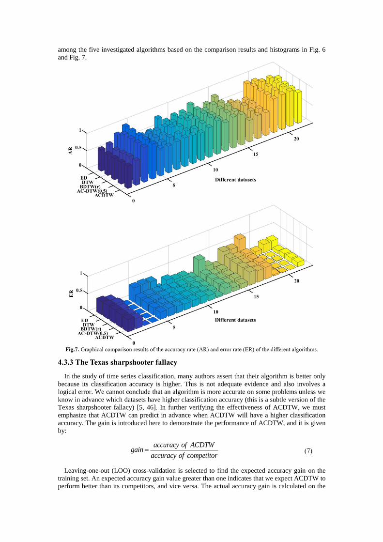
among the five investigated algorithms based on the comparison results and histograms in Fig. 6
and Fig. 7.
Fig.7. Graphical comparison results of the accuracy rate (AR) and error rate (ER) of the different algorithms.
4.3.3 The Texas sharpshooter fallacy
In the study of time series classification, many authors assert that their algorithm is better only
because its classification accuracy is higher. This is not adequate evidence and also involves a
logical error. We cannot conclude that an algorithm is more accurate on some problems unless we
know in advance which datasets have higher classification accuracy (this is a subtle version of the
Texas sharpshooter fallacy) [5, 46]. In further verifying the effectiveness of ACDTW, we must
emphasize that ACDTW can predict in advance when ACDTW will have a higher classification
accuracy. The gain is introduced here to demonstrate the performance of ACDTW, and it is given
by:
accuracy of ACDTWgain
accuracy of competitor
(7)
Leaving-one-out (LOO) cross-validation is selected to find the expected accuracy gain on the training set. An expected accuracy gain value greater than one indicates that we expect ACDTW to
perform better than its competitors, and vice versa. The actual accuracy gain is calculated on the
testing set. Comparing the expected accuracy gain with the actual accuracy gain is the most effective
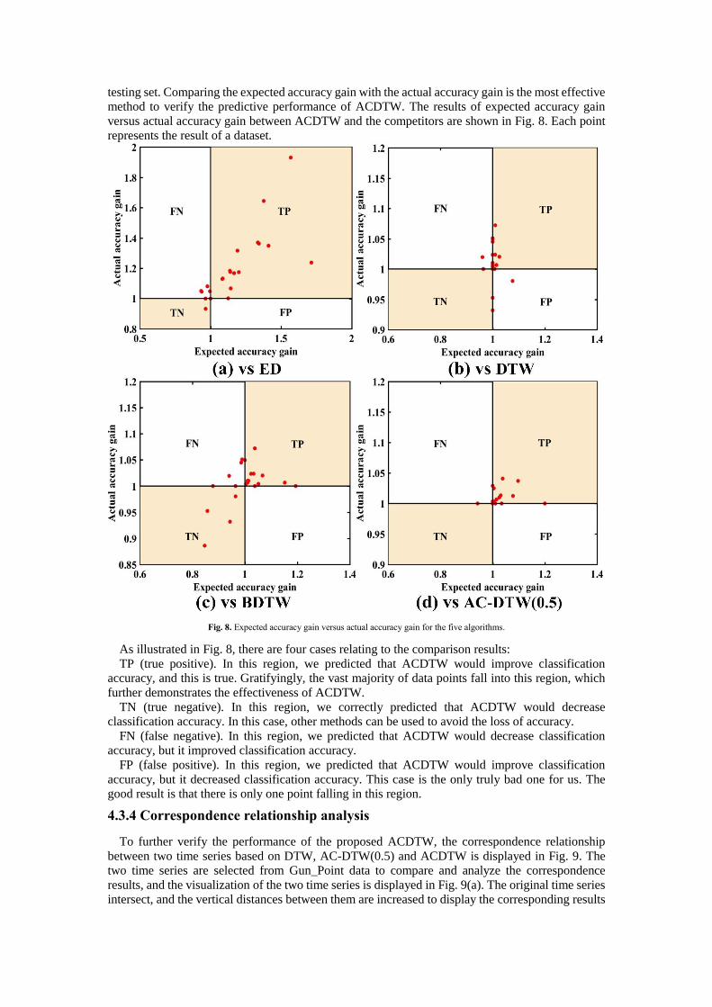
method to verify the predictive performance of ACDTW. The results of expected accuracy gain
versus actual accuracy gain between ACDTW and the competitors are shown in Fig. 8. Each point
represents the result of a dataset.
Fig. 8. Expected accuracy gain versus actual accuracy gain for the five algorithms.
As illustrated in Fig. 8, there are four cases relating to the comparison results:
TP (true positive). In this region, we predicted that ACDTW would improve classification
accuracy, and this is true. Gratifyingly, the vast majority of data points fall into this region, which
further demonstrates the effectiveness of ACDTW.
TN (true negative). In this region, we correctly predicted that ACDTW would decrease
classification accuracy. In this case, other methods can be used to avoid the loss of accuracy.
FN (false negative). In this region, we predicted that ACDTW would decrease classification
accuracy, but it improved classification accuracy.
FP (false positive). In this region, we predicted that ACDTW would improve classification
accuracy, but it decreased classification accuracy. This case is the only truly bad one for us. The
good result is that there is only one point falling in this region.
4.3.4 Correspondence relationship analysis
To further verify the performance of the proposed ACDTW, the correspondence relationship
between two time series based on DTW, AC-DTW(0.5) and ACDTW is displayed in Fig. 9. The
two time series are selected from Gun_Point data to compare and analyze the correspondence
results, and the visualization of the two time series is displayed in Fig. 9(a). The original time series
intersect, and the vertical distances between them are increased to display the corresponding results
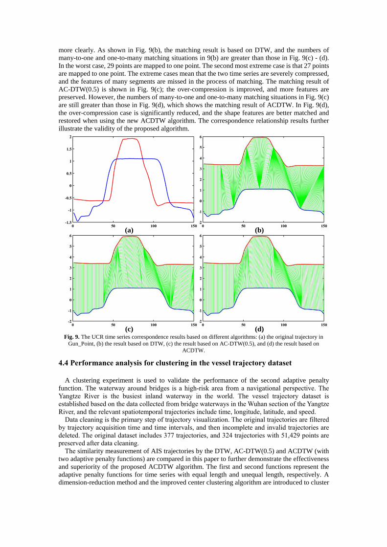
more clearly. As shown in Fig. 9(b), the matching result is based on DTW, and the numbers of
many-to-one and one-to-many matching situations in 9(b) are greater than those in Fig. 9(c) - (d).
In the worst case, 29 points are mapped to one point. The second most extreme case is that 27 points
are mapped to one point. The extreme cases mean that the two time series are severely compressed,
and the features of many segments are missed in the process of matching. The matching result of
AC-DTW(0.5) is shown in Fig. 9(c); the over-compression is improved, and more features are
preserved. However, the numbers of many-to-one and one-to-many matching situations in Fig. 9(c)
are still greater than those in Fig. 9(d), which shows the matching result of ACDTW. In Fig. 9(d),
the over-compression case is significantly reduced, and the shape features are better matched and
restored when using the new ACDTW algorithm. The correspondence relationship results further
illustrate the validity of the proposed algorithm.
(b)(a)
(d)(c)Fig. 9. The UCR time series correspondence results based on different algorithms: (a) the original trajectory in
Gun_Point, (b) the result based on DTW, (c) the result based on AC-DTW(0.5), and (d) the result based on
ACDTW.
4.4 Performance analysis for clustering in the vessel trajectory dataset
A clustering experiment is used to validate the performance of the second adaptive penalty
function. The waterway around bridges is a high-risk area from a navigational perspective. The
Yangtze River is the busiest inland waterway in the world. The vessel trajectory dataset is
established based on the data collected from bridge waterways in the Wuhan section of the Yangtze
River, and the relevant spatiotemporal trajectories include time, longitude, latitude, and speed.
Data cleaning is the primary step of trajectory visualization. The original trajectories are filtered
by trajectory acquisition time and time intervals, and then incomplete and invalid trajectories are
deleted. The original dataset includes 377 trajectories, and 324 trajectories with 51,429 points are
preserved after data cleaning.
The similarity measurement of AIS trajectories by the DTW, AC-DTW(0.5) and ACDTW (with
two adaptive penalty functions) are compared in this paper to further demonstrate the effectiveness
and superiority of the proposed ACDTW algorithm. The first and second functions represent the
adaptive penalty functions for time series with equal length and unequal length, respectively. A dimension-reduction method and the improved center clustering algorithm are introduced to cluster
the vessel trajectories. The detailed experimental process is described in [21] and is not duplicated
in this paper.
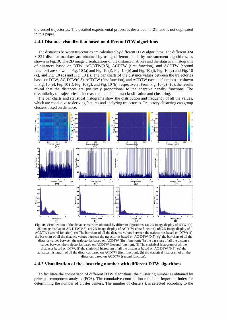
4.4.1 Distance visualization based on different DTW algorithms
The distances between trajectories are calculated by different DTW algorithms. The different 324
× 324 distance matrixes are obtained by using different similarity measurement algorithms, as
shown in Fig.10. The 2D image visualizations of the distance matrixes and the statistical histograms
of distances based on DTW, AC-DTW(0.5), ACDTW (first function), and ACDTW (second
function) are shown in Fig. 10 (a) and Fig. 10 (i), Fig. 10 (b) and Fig. 10 (j), Fig. 10 (c) and Fig. 10
(k), and Fig. 10 (d) and Fig. 10 (l). The bar charts of the distance values between the trajectories
based on DTW, AC-DTW(0.5), ACDTW (first function), and ACDTW (second function) are shown
in Fig. 10 (e), Fig. 10 (f), Fig. 10 (g), and Fig. 10 (h), respectively. From Fig. 10 (a) - (d), the results
reveal that the distances are positively proportional to the adaptive penalty functions. The
dissimilarity of trajectories is increased to facilitate data classification and clustering.
The bar charts and statistical histograms show the distribution and frequency of all the values,
which are conducive to deriving features and analyzing trajectories. Trajectory clustering can group
clusters based on distance.
(i) (j) (k) (l)
(e) (f) (g) (h)
(a) (b) (c) (d)
Fig. 10. Visualization of the distance matrixes obtained by different algorithms. (a) 2D image display of DTW; (b)
2D image display of AC-DTW(0.5); (c) 2D image display of ACDTW (first function); (d) 2D image display of
ACDTW (second function). (e) The bar chart of all the distance values between the trajectories based on DTW; (f)
the bar chart of all the distance values between the trajectories based on AC-DTW (0.5); (g) the bar chart of all the
distance values between the trajectories based on ACDTW (first function); (h) the bar chart of all the distance
values between the trajectories based on ACDTW (second function). (i) The statistical histogram of all the
distances based on DTW; (f) the statistical histogram of all the distances based on AC-DTW (0.5); (g) the
statistical histogram of all the distances based on ACDTW (first function); (h) the statistical histogram of all the
distances based on ACDTW (second function).
4.4.2 Visualization of the clustering number with different DTW algorithms
To facilitate the comparison of different DTW algorithms, the clustering number is obtained by
principal component analysis (PCA). The cumulative contribution rate is an important index for determining the number of cluster centers. The number of clusters k is selected according to the
cumulative contribution rate. If the cumulative contribution rate of the top k principal components
is greater than 95%, then k is the number of clustering centers.
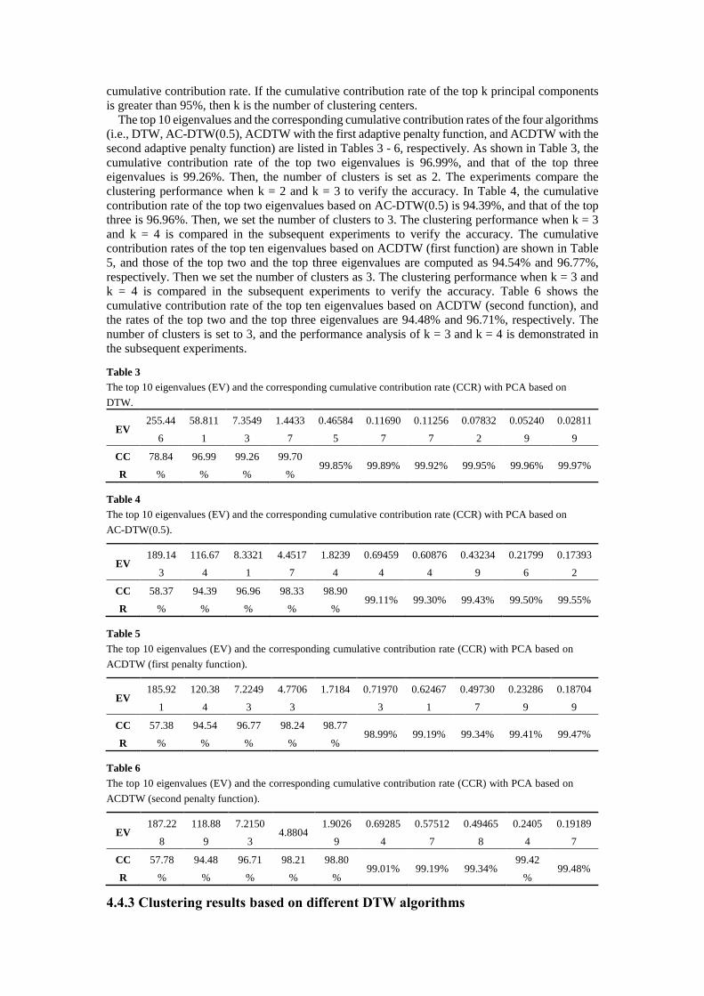
The top 10 eigenvalues and the corresponding cumulative contribution rates of the four algorithms
(i.e., DTW, AC-DTW(0.5), ACDTW with the first adaptive penalty function, and ACDTW with the
second adaptive penalty function) are listed in Tables 3 - 6, respectively. As shown in Table 3, the
cumulative contribution rate of the top two eigenvalues is 96.99%, and that of the top three
eigenvalues is 99.26%. Then, the number of clusters is set as 2. The experiments compare the
clustering performance when k = 2 and k = 3 to verify the accuracy. In Table 4, the cumulative
contribution rate of the top two eigenvalues based on AC-DTW(0.5) is 94.39%, and that of the top
three is 96.96%. Then, we set the number of clusters to 3. The clustering performance when k = 3
and k = 4 is compared in the subsequent experiments to verify the accuracy. The cumulative
contribution rates of the top ten eigenvalues based on ACDTW (first function) are shown in Table
5, and those of the top two and the top three eigenvalues are computed as 94.54% and 96.77%,
respectively. Then we set the number of clusters as 3. The clustering performance when k = 3 and
k = 4 is compared in the subsequent experiments to verify the accuracy. Table 6 shows the
cumulative contribution rate of the top ten eigenvalues based on ACDTW (second function), and
the rates of the top two and the top three eigenvalues are 94.48% and 96.71%, respectively. The
number of clusters is set to 3, and the performance analysis of k = 3 and k = 4 is demonstrated in
the subsequent experiments.
Table 3
The top 10 eigenvalues (EV) and the corresponding cumulative contribution rate (CCR) with PCA based on
DTW.
EV 255.44
6
58.811
1
7.3549
3
1.4433
7
0.46584
5
0.11690
7
0.11256
7
0.07832
2
0.05240
9
0.02811
9
CC
R
78.84
%
96.99
%
99.26
%
99.70
% 99.85% 99.89% 99.92% 99.95% 99.96% 99.97%
Table 4
The top 10 eigenvalues (EV) and the corresponding cumulative contribution rate (CCR) with PCA based on
AC-DTW(0.5).
EV 189.14
3
116.67
4
8.3321
1
4.4517
7
1.8239
4
0.69459
4
0.60876
4
0.43234
9
0.21799
6
0.17393
2
CC
R
58.37
%
94.39
%
96.96
%
98.33
%
98.90
% 99.11% 99.30% 99.43% 99.50% 99.55%
Table 5
The top 10 eigenvalues (EV) and the corresponding cumulative contribution rate (CCR) with PCA based on
ACDTW (first penalty function).
EV 185.92
1
120.38
4
7.2249
3
4.7706
3
1.7184 0.71970
3
0.62467
1
0.49730
7
0.23286
9
0.18704
9
CC
R
57.38
%
94.54
%
96.77
%
98.24
%
98.77
% 98.99% 99.19% 99.34% 99.41% 99.47%
Table 6
The top 10 eigenvalues (EV) and the corresponding cumulative contribution rate (CCR) with PCA based on
ACDTW (second penalty function).
EV 187.22
8
118.88
9
7.2150
3 4.8804
1.9026
9
0.69285
4
0.57512
7
0.49465
8
0.2405
4
0.19189
7
CC
R
57.78
%
94.48
%
96.71
%
98.21
%
98.80
% 99.01% 99.19% 99.34%
99.42
% 99.48%
4.4.3 Clustering results based on different DTW algorithms
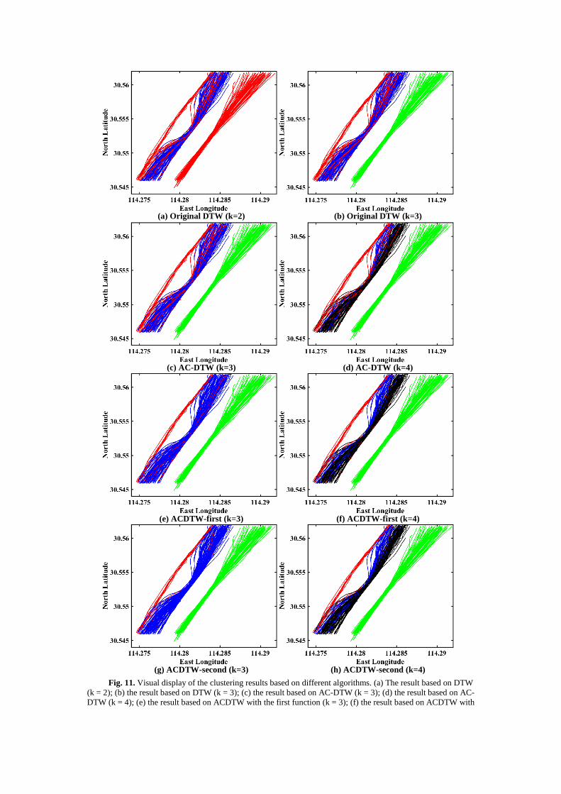
The clustering results based on different DTW algorithms are shown in Fig. 11. The performance
of the four algorithms, (i.e., DTW, AC-DTW(0.5), ACDTW with the first adaptive penalty function,
and ACDTW with the second adaptive penalty function) are compared and analyzed in detail. The
clustering results based on DTW are shown in Fig. 11 (a) - (b), indicating poor performance on k =
2 and k = 3. Fig. 11 (c) - (d) show that the performance of clustering results based on AC-DTW(0.5)
is better than that in Fig. 11 (a) - (b), showing that AC-DTW(0.5) is more effective than DTW in
vessel trajectory clustering. Additionally, the clustering performance when k = 3 is better than that
when k = 4, as shown in Fig. 11 (c) - (d). The red, blue and green trajectories represent different
classes in Fig. 11 (c). However, it is noteworthy that 20 trajectories are misclassified. The red
trajectories among the blue trajectories are misclassified. The red, blue, black, and green trajectories
represent different classes in Fig. 11 (d). The red trajectories among the blue and black trajectories
are misclassified.
There are many differences in the lengths of vessel trajectories, so the clustering performance
based on ACDTW with two penalty functions is also compared in the experiments. The clustering
results based on ACDTW with the first penalty function are shown in Fig. 11 (e) - (f), revealing
better performance than DTW and AC-DTW(0.5). The clustering results show the effectiveness and
reasonability of using ACDTW with the first function. Additionally, the clustering performance
when k = 3 is better than that when k = 4, as shown in Fig. 11 (e) - (f). The red, blue and green
trajectories represent different classes in Fig. 11 (e). The six red trajectories among the blue
trajectories are misclassified. The red, blue, black, and green trajectories represent different classes
in Fig. 11 (f), and the six red trajectories among the blue and black trajectories are misclassified.
From Fig. 11 (g) - (h), the clustering performance based on ACDTW with the second function is
better than the results of the other three algorithms. This further verifies the effectiveness and
reasonability of using ACDTW with the second function. Furthermore, the clustering result when k
= 3 is better than that when k = 4, as shown in Fig. 11 (g) - (h). Four trajectories are misclassified.
The red, blue and green trajectories represent different classes in Fig. 11 (g). The four red trajectories
among the blue trajectories are misclassified. The red, blue, black, and green trajectories represent
different classes in Fig. 11 (h), and the four red trajectories among the blue and black trajectories
are misclassified.
Based on the comparison and analysis in Fig. 11, the performance ranking of the four algorithms
is in declining order of ACDTW with the second penalty function, ACDTW with the first penalty
function, AC-DTW(0.5), and DTW.
(a) Original DTW (k=2) (b) Original DTW (k=3)
(c) AC-DTW (k=3) (d) AC-DTW (k=4)
(e) ACDTW-first (k=3) (f) ACDTW-first (k=4)
(g) ACDTW-second (k=3) (h) ACDTW-second (k=4) Fig. 11. Visual display of the clustering results based on different algorithms. (a) The result based on DTW
(k = 2); (b) the result based on DTW (k = 3); (c) the result based on AC-DTW (k = 3); (d) the result based on AC-
DTW (k = 4); (e) the result based on ACDTW with the first function (k = 3); (f) the result based on ACDTW with
the first function (k = 4); (g) the result based on ACDTW with the second function (k = 3); (h) the result based on
ACDTW with the second function (k = 4).
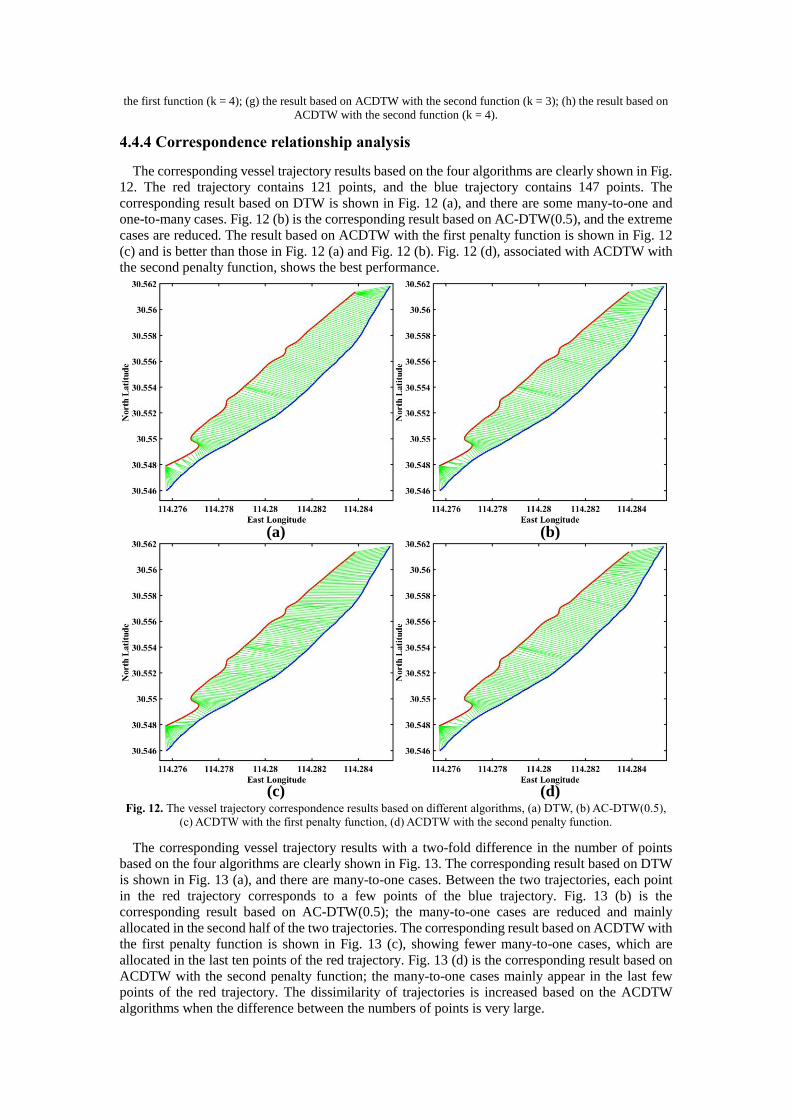
4.4.4 Correspondence relationship analysis
The corresponding vessel trajectory results based on the four algorithms are clearly shown in Fig.
12. The red trajectory contains 121 points, and the blue trajectory contains 147 points. The
corresponding result based on DTW is shown in Fig. 12 (a), and there are some many-to-one and
one-to-many cases. Fig. 12 (b) is the corresponding result based on AC-DTW(0.5), and the extreme
cases are reduced. The result based on ACDTW with the first penalty function is shown in Fig. 12
(c) and is better than those in Fig. 12 (a) and Fig. 12 (b). Fig. 12 (d), associated with ACDTW with
the second penalty function, shows the best performance.
(b)(a)
(d)(c) Fig. 12. The vessel trajectory correspondence results based on different algorithms, (a) DTW, (b) AC-DTW(0.5),
(c) ACDTW with the first penalty function, (d) ACDTW with the second penalty function.
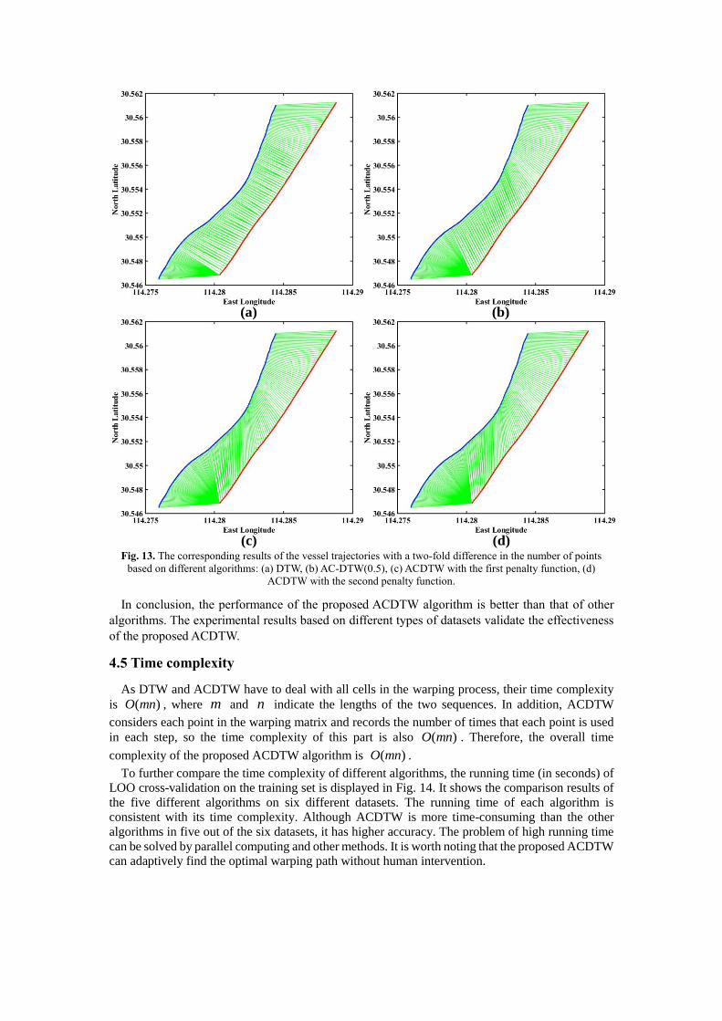
The corresponding vessel trajectory results with a two-fold difference in the number of points
based on the four algorithms are clearly shown in Fig. 13. The corresponding result based on DTW
is shown in Fig. 13 (a), and there are many-to-one cases. Between the two trajectories, each point
in the red trajectory corresponds to a few points of the blue trajectory. Fig. 13 (b) is the
corresponding result based on AC-DTW(0.5); the many-to-one cases are reduced and mainly
allocated in the second half of the two trajectories. The corresponding result based on ACDTW with
the first penalty function is shown in Fig. 13 (c), showing fewer many-to-one cases, which are
allocated in the last ten points of the red trajectory. Fig. 13 (d) is the corresponding result based on
ACDTW with the second penalty function; the many-to-one cases mainly appear in the last few points of the red trajectory. The dissimilarity of trajectories is increased based on the ACDTW
algorithms when the difference between the numbers of points is very large.
(b)
(d)
(a)
(c) Fig. 13. The corresponding results of the vessel trajectories with a two-fold difference in the number of points
based on different algorithms: (a) DTW, (b) AC-DTW(0.5), (c) ACDTW with the first penalty function, (d)
ACDTW with the second penalty function.
In conclusion, the performance of the proposed ACDTW algorithm is better than that of other
algorithms. The experimental results based on different types of datasets validate the effectiveness
of the proposed ACDTW.
4.5 Time complexity
As DTW and ACDTW have to deal with all cells in the warping process, their time complexity
is ( )O mn , where m and n indicate the lengths of the two sequences. In addition, ACDTW
considers each point in the warping matrix and records the number of times that each point is used
in each step, so the time complexity of this part is also ( )O mn . Therefore, the overall time
complexity of the proposed ACDTW algorithm is ( )O mn .
To further compare the time complexity of different algorithms, the running time (in seconds) of
LOO cross-validation on the training set is displayed in Fig. 14. It shows the comparison results of
the five different algorithms on six different datasets. The running time of each algorithm is
consistent with its time complexity. Although ACDTW is more time-consuming than the other
algorithms in five out of the six datasets, it has higher accuracy. The problem of high running time
can be solved by parallel computing and other methods. It is worth noting that the proposed ACDTW
can adaptively find the optimal warping path without human intervention.
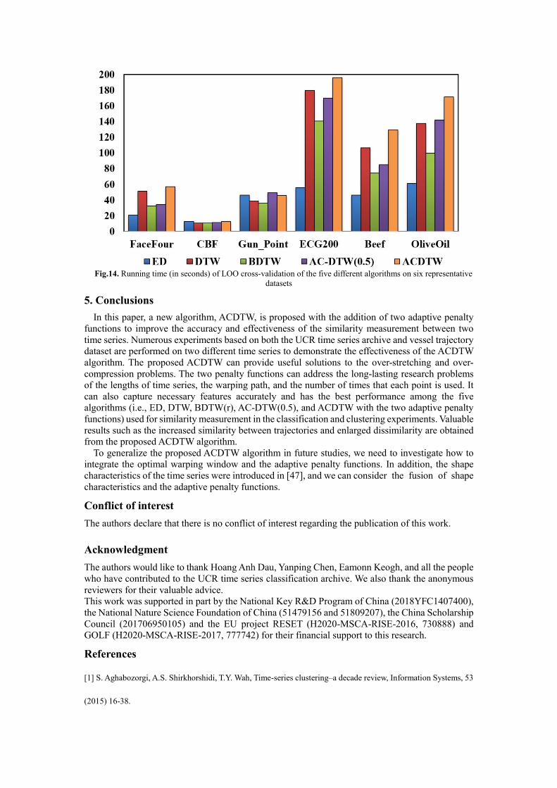
Fig.14. Running time (in seconds) of LOO cross-validation of the five different algorithms on six representative
datasets
5. Conclusions
In this paper, a new algorithm, ACDTW, is proposed with the addition of two adaptive penalty
functions to improve the accuracy and effectiveness of the similarity measurement between two
time series. Numerous experiments based on both the UCR time series archive and vessel trajectory
dataset are performed on two different time series to demonstrate the effectiveness of the ACDTW
algorithm. The proposed ACDTW can provide useful solutions to the over-stretching and over-
compression problems. The two penalty functions can address the long-lasting research problems
of the lengths of time series, the warping path, and the number of times that each point is used. It
can also capture necessary features accurately and has the best performance among the five
algorithms (i.e., ED, DTW, BDTW(r), AC-DTW(0.5), and ACDTW with the two adaptive penalty
functions) used for similarity measurement in the classification and clustering experiments. Valuable
results such as the increased similarity between trajectories and enlarged dissimilarity are obtained
from the proposed ACDTW algorithm.
To generalize the proposed ACDTW algorithm in future studies, we need to investigate how to
integrate the optimal warping window and the adaptive penalty functions. In addition, the shape
characteristics of the time series were introduced in [47], and we can consider the fusion of shape
characteristics and the adaptive penalty functions.
Conflict of interest
The authors declare that there is no conflict of interest regarding the publication of this work.
Acknowledgment
The authors would like to thank Hoang Anh Dau, Yanping Chen, Eamonn Keogh, and all the people
who have contributed to the UCR time series classification archive. We also thank the anonymous
reviewers for their valuable advice.
This work was supported in part by the National Key R&D Program of China (2018YFC1407400),
the National Nature Science Foundation of China (51479156 and 51809207), the China Scholarship
Council (201706950105) and the EU project RESET (H2020-MSCA-RISE-2016, 730888) and
GOLF (H2020-MSCA-RISE-2017, 777742) for their financial support to this research.
References
[1] S. Aghabozorgi, A.S. Shirkhorshidi, T.Y. Wah, Time-series clustering–a decade review, Information Systems, 53
(2015) 16-38.
[2] R. Al-Zaidi, J.C. Woods, M. Al-Khalidi, H.S. Hu, Building novel VHF-based wireless sensor networks for the
Internet of marine things, IEEE Sensors Journal, 18 (2018) 2131-2144.
[3] S. Atev, G. Miller, N.P. Papanikolopoulos, Clustering of vehicle trajectories, IEEE transactions on intelligent
transportation systems, 11 (2010) 647-657.
[4] S. Barbon, R.C. Guido, L.S. Vieira, E.S. Fonseca, F.L. Sanchez, P.R. Scalassara, C.D. Maciel, J.C. Pereira, S.H.
Chen, Wavelet-based dynamic time warping, Journal of Computational and Applied Mathematics, 227 (2009) 271-
287.
[5] G.E. Batista, E.J. Keogh, O.M. Tataw, V.M. De Souza, CID: an efficient complexity-invariant distance for time
series, Data Mining and Knowledge Discovery, 28 (2014) 634-669.
[6] D.J. Berndt, J. Clifford, Using dynamic time warping to find patterns in time series, in: Proc. of the 3rd
International Conference on Knowledge Discovery and Data Mining, Seattle, WA, 1994, pp. 359-370.
[7] Y. Cai, H. Wang, X. Chen, H. Jiang, Trajectory-based anomalous behaviour detection for intelligent traffic
surveillance, IET Intelligent Transport Systems, 9 (2015) 810-816.
[8] Y. Chen, E. Keogh, B. Hu, N. Begum, A. Bagnall, A. Mueen, G. Batista, The UCR time series classification
archive, (2015) URL: www. cs. ucr. edu/~ eamonn/time_series_data.
[9] M.Y. Choong, R.K.Y. Chin, K.B. Yeo, K.T.K. Teo, Trajectory pattern mining via clustering based on similarity
function for transportation surveillance, International Journal of Simulation-Systems, Science & Technology, 17
(2016) 19.11-19.17.
[10] H.A. Dau, A. Bagnall, K. Kamgar, C.-C.M. Yeh, Y. Zhu, S. Gharghabi, C.A. Ratanamahatana, E. Keogh, The
UCR time series archive, arXiv preprint arXiv:1810.07758, (2018).
[11] D. Folgado, M. Barandas, R. Matias, R. Martins, M. Carvalho, H. Gamboa, Time alignment measurement for
time series, Pattern Recognition, 81 (2018) 268-279.
[12] T. Gorecki, M. Luczak, Using derivatives in time series classification, Data Mining and Knowledge Discovery,
26 (2013) 310-331.
[13] C. Gupta, A. Jain, D.K. Tayal, O. Castillo, ClusFuDE: Forecasting low dimensional numerical data using an
improved method based on automatic clustering, fuzzy relationships and differential evolution, Engineering
Applications of Artificial Intelligence, 71 (2018) 175-189.
[14] Y. Han, L. Zhu, Z. Cheng, J. Li, X. Liu, Discrete optimal graph clustering, IEEE Transactions on Cybernetics,
50 (2020) 1697-1710.
[15] B. Herbst, H. Coetzer, On an offline signature verification system, in: Proc. of the 9th Annual South African
Workshop on Pattern Recognition, 1998, pp. 39-43.
[16] F. Itakura, Minimum prediction residual principle applied to speech recognition, IEEE T Acoust Speech, 23
(1975) 67-72.
[17] Y.S. Jeong, M.K. Jeong, O.A. Omitaomu, Weighted dynamic time warping for time series classification, Pattern
Recognition, 44 (2011) 2231-2240.
[18] E.J. Keogh, M.J. Pazzani, Derivative dynamic time warping, in: Proc. of the 2001 SIAM International
Conference on Data Mining, 2001, pp. 1-11.
[19] M. Krawczak, G. Szkatuła, An approach to dimensionality reduction in time series, Information Sciences, 260
(2014) 15-36.
[20] J.S.L. Lam, K.P.B. Cullinane, P.T.-W. Lee, The 21st-century Maritime Silk Road: challenges and opportunities
for transport management and practice, Transport Reviews, 38 (2018) 413-415.
[21] H. Li, J. Liu, R. Liu, N. Xiong, K. Wu, T. Kim, A dimensionality reduction-based multi-step clustering method
for robust vessel trajectory analysis, Sensors, 17 (2017) 1792.
[22] H. Li, J. Liu, K. Wu, Z. Yang, R. Liu, N. Xiong, Spatio-temporal vessel trajectory clustering based on data
mapping and density, IEEE Access, 6 (2018) 58939-58954.
[23] T.W. Liao, Clustering of time series data—a survey, Pattern recognition, 38 (2005) 1857-1874.
[24] J. Lines, A. Bagnall, Time series classification with ensembles of elastic distance measures, Data Mining and
Knowledge Discovery, 29 (2015) 565-592.
[25] J. Liu, H. Li, Z. Yang, K. Wu, Y. Liu, R.W. Liu, Adaptive Douglas-Peucker algorithm with automatic
thresholding for AIS-based vessel trajectory compression, IEEE Access, 7 (2019) 150677-150692.
[26] W.-K. Loh, S. Mane, J. Srivastava, Mining temporal patterns in popularity of web items, Information Sciences,
181 (2011) 5010-5028.
[27] M. Morel, C. Achard, R. Kulpa, S. Dubuisson, Time-series averaging using constrained dynamic time warping
with tolerance, Pattern Recognition, 74 (2018) 77-89.
[28] B. Morris, M. Trivedi, Learning trajectory patterns by clustering: Experimental studies and comparative
evaluation, in: 2009 IEEE Conference on Computer Vision and Pattern Recognition, Miami, FL, USA, 2009, pp.
312-319.
[29] V. Niennattrakul, C.A. Ratanamahatana, On clustering multimedia time series data using k-means and dynamic
time warping, in: 2007 International Conference on Multimedia and Ubiquitous Engineering (MUE'07), Seoul,
Korea, 2007, pp. 733-738.
[30] F. Petitjean, G. Forestier, G.I. Webb, A.E. Nicholson, Y.P. Chen, E. Keogh, Faster and more accurate
classification of time series by exploiting a novel dynamic time warping averaging algorithm, Knowledge and
Information Systems, 47 (2016) 1-26.
[31] R. Saini, P.P. Roy, D.P. Dogra, A novel point-line duality feature for trajectory classification, The Visual
Computer, 35 (2019) 415-427.
[32] H. Sakoe, S. Chiba, Dynamic-programming algorithm optimization for spoken word recognition, IEEE
Transactions on Acoustics Speech and Signal Processing, 26 (1978) 43-49.
[33] S. Salvador, P. Chan, Toward accurate dynamic time warping in linear time and space, Intelligent Data Analysis,
11 (2007) 561-580.
[34] A.P. Shanker, A.N. Rajagopalan, Off-line signature verification using DTW, Pattern Recognition Letters, 28
(2007) 1407-1414.
[35] A. Sharma, S. Sundaram, An enhanced contextual DTW based system for online signature verification using
Vector Quantization, Pattern Recognition Letters, 84 (2016) 22-28.
[36] D.F. Silva, R. Giusti, E. Keogh, G.E.A.P.A. Batista, Speeding up similarity search under dynamic time warping
by pruning unpromising alignments, Data Mining and Knowledge Discovery, 32 (2018) 988-1016.
[37] J. Soto, O. Castillo, P. Melin, W. Pedrycz, A new approach to multiple time series prediction using MIMO fuzzy
aggregation models with Modular Neural Networks, International Journal of Fuzzy Systems, 21 (2019) 1629-1648.
[38] F. Tu, S.S. Ge, Y.S. Choo, C.C. Hang, Sea state identification based on vessel motion response learning via
multi-layer classifiers, Ocean Engineering, 147 (2018) 318-332.
[39] V.M. Velichko, N.G. Zagoruyko, Automatic recognition of 200 words, International Journal of Man-Machine
Studies, 2 (1970) 223-234.
[40] Y. Wan, X. Chen, Y. Shi, Adaptive cost dynamic time warping distance in time series analysis for classification,
Journal of Computational and Applied Mathematics, 319 (2017) 514-520.
[41] M. Yoshimural, I. Yoshimura, An application of the sequential dynamic programming matching method to off-
line signature verification, in, Springer Berlin Heidelberg, Berlin, Heidelberg, 1997, pp. 299-310.
[42] C. Yu, L. Luo, L.L.-H. Chan, T. Rakthanmanon, S. Nutanong, A fast LSH-based similarity search method for
multivariate time series, Information Sciences, 476 (2019) 337-356.
[43] G. Yuan, P.H. Sun, J. Zhao, D.X. Li, C.W. Wang, A review of moving object trajectory clustering algorithms,
Artificial Intelligence Review, 47 (2017) 123-144.
[44] J. Zhang, H. Li, Q. Gao, H. Wang, Y. Luo, Detecting anomalies from big network traffic data using an adaptive
detection approach, Information Sciences, 318 (2015) 91-110.
[45] W. Zhang, F. Goerlandt, J. Montewka, P. Kujala, A method for detecting possible near miss ship collisions from
AIS data, Ocean Engineering, 107 (2015) 60-69.
[46] Z. Zhang, R. Tavenard, A. Bailly, X. Tang, P. Tang, T. Corpetti, Dynamic time warping under limited warping
path length, Information Sciences, 393 (2017) 91-107.
[47] J. Zhao, L. Itti, Shapedtw: shape dynamic time warping, Pattern Recognition, 74 (2018) 171-184.
[48] L. Zhao, G. Shi, A novel similarity measure for clustering vessel trajectories based on Dynamic Time Warping,
The Journal of Navigation, 72 (2019) 290-306.
[49] L. Zhao, G. Shi, A trajectory clustering method based on Douglas-Peucker compression and density for marine
traffic pattern recognition, Ocean Engineering, 172 (2019) 456-467.
[50] Y. Zheng, Trajectory data mining: an overview, ACM Transactions on Intelligent Systems and Technology, 6
(2015) 1-41.


