arX

iv:m

ath-

ph/0

1040

24v2

9 N

ov 2

001

Adiabatic Decoupling and Time-Dependent Born-Oppenheimer

Theory

Herbert Spohn and Stefan Teufel

Zentrum Mathematik and Physik Department,

Technische Universitat Munchen,

80290 Munchen, Germany

email: spohn@ma.tum.de, teufel@ma.tum.de

July 9, 2001

Abstract

We reconsider the time-dependent Born-Oppenheimer theory with the goal to carefullyseparate between the adiabatic decoupling of a given group of energy bands from theirorthogonal subspace and the semiclassics within the energy bands. Band crossings are allowedand our results are local in the sense that they hold up to the first time when a band crossingis encountered. The adiabatic decoupling leads to an effective Schrodinger equation for thenuclei, including contributions from the Berry connection.

1 Introduction

Molecules consist of light electrons, mass me, and heavy nuclei, mass M which depends onthe type of nucleus. Born and Oppenheimer [3] wanted to explain some general features ofmolecular spectra and realized that, since the ratio me/M is small, it could be used as anexpansion parameter for the energy levels of the molecular Hamiltonian. The time-independentBorn-Oppenheimer theory has been put on firm mathematical grounds by Combes, Duclos, andSeiler [5], Hagedorn [8], and more recently in [16].

With the development of tailored state preparation and ultra precise time resolution there isa growing interest in understanding and controlling the dynamics of molecules, which requiresan analysis of the solutions to the time-dependent Schrodinger equation, again exploiting thatme/M is small. The molecular Hamiltonian is of the form

H =~

2

2me

(− i∇x −Aext(x)

)2+

~2

2M

(− i∇X +Aext(X)

)2+ Ve(x) + Ven(X,x) + Vn(X) . (1)

For notational simplicity we ignore spin degrees of freedom and assume that all nuclei havethe same mass. We have k electrons with positions x1, . . . , xk = x and l nuclei with positionsX1, . . . ,Xl = X. The first and second term of H are the kinetic energies of the electrons and ofthe nuclei, respectively. An external magnetic field is included through the vector potential Aext.Electrons and nuclei interact via the static Coulomb potential. Therefore Ve is the electronic,Vn the nucleonic repulsion, and Ven the attraction between electrons and nuclei. Ve and Vn mayalso contain an external electrostatic potential.

1

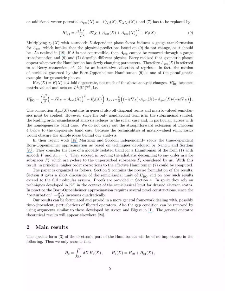
(R)

RR0

H (R)σ( )e

E (R)2

E (R)3

E (R)1

Σ

Figure 1: The schematic spectrum of He(R) for a diatomic molecule as a function of the sepa-ration R of the two nuclei.

In atomic units (me = ~ = 1) the Hamiltonian (1) can be written more concisely as

H =me

M

1

2

(− i∇X +Aext(X)

)2+He(X) , (2)

emphasizing that the nuclear kinetic energy will be treated as a “small perturbation”. He(X)is the electronic Hamiltonian for given position X of the nuclei,

He(X) =1

2

(− i∇x −Aext(x)

)2+ Ve(x) + Ven(X,x) + Vn(X) . (3)

He(X) is a self-adjoint operator on the electronic Hilbert space L2(R3k) restricted to its antisym-metric subspace. Later on we will need some smoothness of He(X), which can be establishedeasily if the electrons are treated as point-like and the nuclei have an extended, rigid chargedistribution.

Generically He(X) has, possibly degenerate, eigenvalues E1(X) < E2(X) < . . . which termi-nate at the continuum edge Σ(X). Thereby one obtains the band structure as plotted schemat-ically in Figure 1. The discrete bands Ej(X) may cross and possibly merge into the continuousspectrum as indicated in Figure 2.

Comparing kinetic energies, we find for the speeds |vn| ≈ (me/M)1/2|ve|, which means thaton the atomic scale the nuclei move very slowly. If we regard X(t) as a given nucleonic trajectory,then He(X(t)) is a Hamiltonian with slow time variation and the time-adiabatic theorem [15, 14,1] can be applied [2]. For us X are quantum mechanical degrees of freedom. The Hamiltonian Hof (2) is time-independent and we can only exploit that the nucleonic Laplacian carries a smallprefactor. To distinguish, we refer to our situation as space-adiabatic. Since the nuclei movevery slowly, their dynamics must be followed over sufficiently long times. From the speed ratiowe conclude that these times are of order (me/M)1/2 in atomic units. To simplify notation wedefine

ε =

√me

M(4)

as the small dimensionless parameter. Then

Hε = ε21

2

(− i∇X +Aext(X)

)2+He(X) , (5)

2

and we want to study the solutions of the time-dependent Schrodinger equation

iε∂ψ

∂t= Hεψ (6)

in the limit of small ε.The crude physical picture underlying the analysis of (6) is that the nuclei behave semiclas-

sically because of their large mass and that the electrons rapidly adjust to the slow nucleonicmotion. Thus, in fact, the time-dependent Born-Oppenheimer approximation involves two lim-its. If the electrons are initially in the eigenstate χj(X0) of the j-th band with energy Ej(X0),where X0 is the approximate initial configuration of the nuclei, then the j-th band is adiabati-cally protected provided there is an energy gap separating it from the rest of the spectrum. Thusat later times, up to small error, the electronic wave function is still in the subspace correspond-ing to the j-th band. But this implies that the nuclei are governed by the Born-OppenheimerHamiltonian

HεBO = ε2

1

2

(− i∇X +Aext(X)

)2+ Ej(X) . (7)

Since ε ≪ 1, HεBO can be analyzed through semiclassical methods where to leading order the

contributions come from the classical flow Φt corresponding to the classical Hamiltonian HclBO =

12p

2 +Ej(q) on nucleonic phase space.In general, Ej(X) may touch another band as X varies. To allow for such band crossings we

introduce the region Λ ⊂ Rn, n = 3l, in nucleonic configuration space, such that Ej restricted

to Λ does not cross or touch any other energy band. The classical flow Φt then has Λ × Rn as

phase space and is defined only up to the time when it first hits the boundary ∂Λ × Rn. Up to

that time (7) still correctly describes the quantum evolution. To follow the tunneling througha band crossing other methods have to be used [11, 7], in particular, the codimension of thecrossing is of relevance.

The mathematical investigation of the time-dependent Born-Oppenheimer theory was ini-tiated and carried out in great detail by Hagedorn. In his pioneering work [9] he constructsapproximate solutions to (6) of the form φq(t),p(t) ⊗ χj(q(t)), where φq(t),p(t) is a coherent statecarried along the classical flow, (q(t), p(t)) = Φt(q0, p0). The difference to the true solutionwith the same initial condition is of order

√ε in the L2-norm over times of order ε−1 in atomic

units and the approximation holds until the first hitting time of ∂Λ × Rn. In a recent work

Hagedorn and Joye [10] construct solutions to (6) satisfying exponentially small error estimates.In Hagedorn’s approach the “adiabatic and semiclassical limits are being taken simultaneously,and they are coupled [10]”.

In our paper we carefully separate the space-adiabatic and the semiclassical limit. Oneimmediate benefit is the generalization of the first order analysis of Hagedorn from coherentstates to arbitrary wave functions.

Let us explain our result for the space-adiabatic part in more detail. We assume that thereis some region Λ ⊂ R

n in the nucleonic configuration space, such that some subset σ∗(X) ofσ(He(X)) is separated from the remainder of the spectrum by a gap for all X ∈ Λ, i.e.

dist(σ∗(X), σ(He(X)) \ σ∗(X)) ≥ d > 0 for all X ∈ Λ .

Λ could be punctured by small balls (for n = 2) because of band crossings. Λ could also terminatebecause the point spectrum merges in the continuum, which physically means that the moleculeloses an electron through ionization. Let P∗(X) be the spectral projection of He(X) associatedwith σ∗(X) and P∗ =

∫ ⊕Λ dX P∗(X). We will establish that the unitary time evolution e−iHεt/ε

3

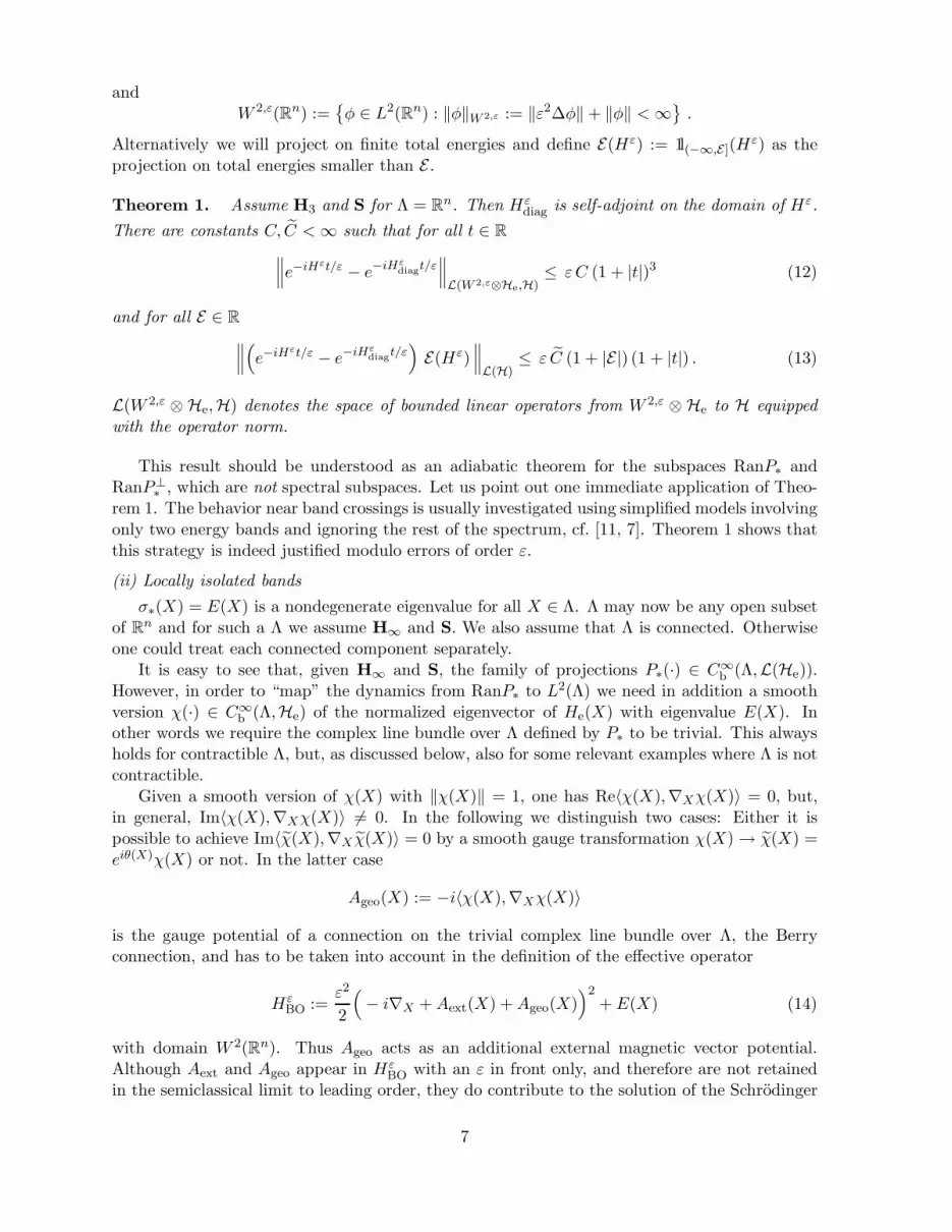
X*

σ ( )

σ( )H (X)e

XΛ

RanP

a)

a)

b)

b)

*

Figure 2: The wave function can leave RanP∗ in two different ways. Either by transitions toother bands (a) or through the boundary of Λ (b).

agrees on RanP∗ with the diagonal evolution e−iHεdiagt/ε generated by Hε

diag := P∗HεP∗ up to

errors of order ε as long as the leaking through the boundary of Λ is sufficiently small.To complete the analysis one has to control the flow of the wave function through ∂Λ. One

possibility is to simply avoid the problem by assuming that Λ = Rn, hence ∂Λ = ∅. We will

refer to this case as a globally isolated band. Of course, the set (X, y) ∈ Rn × R : y ∈ σ∗(X)

may contain arbitrary band crossings. As one of our main results, we prove that the subspaceRanP∗ is adiabatically protected. In particular for the purpose of studying band crossings thefull molecular Hamiltonian may be replaced by a simplified model with two bands only.

In general one has ∂Λ 6= ∅, to which we refer as a locally isolated band. To estimate theflow out of Λ the only technique available seems to be semiclassical analysis. But this requires acontrol over the semiclassical evolution, for which one needs, at present, that (X, y) ∈ Λ × R :y ∈ σ∗(X) contains no band crossings. Then (X, y) ∈ Λ × R : y ∈ σ∗(X) = ∪j (X, y) ∈Λ × R : y = Ej(X) is the disjoint union of possibly degenerate energy bands Ej(X). We willprove that each band separately is adiabatically protected.

In the special case where σ∗(X) = Ej(X) is a nondegenerate eigenvalue for X ∈ Λ, e−iHεdiagt/ε

is well approximated through e−iHεBOt/ε on L2(Rn). Since Hε

BO is a standard semiclassicaloperator, one can easily control the X-support of the wave function and therefore prove a resultfor rather general Λ ⊂ R

n, for the details see Theorem 4. Roughly speaking, it says that if φt isa solution of the effective Schrodinger equation for the nuclei

iε∂φt

∂t= Hε

BOφt , (8)

with suppφ0 ⊂ Λ, then, modulo an error of order ε,

ψt := φt(X)χj(X,x)

is a solution of the full Schrodinger equation (6) with initial condition ψ0(X,x) = φ0(X)χj(X,x)as long as φt is supported in Λ up to L2-mass of order ε. This maximal time span can becomputed using the classical flow Φt.

As first observed by Mead and Truhlar [19], in generalHεBO acquires as a first order correction

4

an additional vector potential Ageo(X) = −i〈χj(X),∇Xχj(X)〉 and (7) has to be replaced by

HεBO = ε2

1

2

(− i∇X +Aext(X) +Ageo(X)

)2+ Ej(X) . (9)

Multiplying χj(X) with a smooth X-dependent phase factor induces a gauge transformationfor Ageo, which implies that the physical predictions based on (9) do not change, as it shouldbe. As noticed in [19], if Λ is not contractible, then Ageo cannot be removed through a gaugetransformation and (9) and (7) describe different physics. Berry realized that geometric phasesappear whenever the Hamiltonian has slowly changing parameters. Therefore Ageo(X) is referredto as Berry connection, cf. [22] for an instructive collection of reprints. In fact, the motionof nuclei as governed by the Born-Oppenheimer Hamiltonian (9) is one of the paradigmaticexamples for geometric phases.

If σ∗(X) = E(X) is k-fold degenerate, not much of the above analysis changes. HεBO becomes

matrix-valued and acts on L2(Rn)⊕k, i.e.

HεBO =

(ε2

2

(− i∇X +Aext(X)

)2+ Ej(X)

)1k×k+

ε

2

((−iε∇X)·Ageo(X)+Ageo(X)·(−iε∇X )

).

The connection Ageo(X) contains in general also off-diagonal terms and matrix-valued semiclas-sics must be applied. However, since the only nondiagonal term is in the subprincipal symbol,the leading order semiclassical analysis reduces to the scalar case and, in particular, agrees withthe nondegenerate band case. We do not carry out the straightforward extension of Theorem4 below to the degenerate band case, because the technicalities of matrix-valued semiclassicswould obscure the simple ideas behind our analysis.

In their recent work [18] Martinez and Sordoni independently study the time-dependentBorn-Oppenheimer approximation as based on techniques developed by Nenciu and Sordoni[20]. They consider the case of a globally isolated band for a Hamiltonian of the form (1) withsmooth V and Aext = 0. They succeed in proving the adiabatic decoupling to any order in ε forsubspaces P ε

∗ which are ε-close to the unperturbed subspaces P∗ considered by us. With thisresult, in principle, higher order corrections to the effective Hamiltonian (7) could be computed.

The paper is organized as follows. Section 2 contains the precise formulation of the results.Section 3 gives a short discussion of the semiclassical limit of Hε

BO and on how such resultsextend to the full molecular system. Proofs are provided in Section 4. In spirit they rely ontechniques developed in [23] in the context of the semiclassical limit for dressed electron states.In practice the Born-Oppenheimer approximation requires several novel constructions, since the“perturbation” − ε2

2 ∆ increases quadratically.Our results can be formulated and proved in a more general framework dealing with, possibly

time-dependent, perturbations of fibered operators. Also the gap condition can be removed byusing arguments similar to those developed by Avron and Elgart in [1]. The general operatortheoretical results will appear elsewhere [24].

2 Main results

The specific form (3) of the electronic part of the Hamiltonian will be of no importance in thefollowing. Thus we only assume that

He =

∫ ⊕

Rn

dX He(X) , He(X) = He0 +He1(X) ,

5

where He0 is self-adjoint on some dense domain D ⊂ He and bounded from below and He1(X) ∈L(He) is a continuous family of self-adjoint operators, bounded uniformly for X ∈ R

n. ThusHe is self-adjoint on D(He) = L2(Rn) ⊗ D ⊂ H := L2(Rn) ⊗ He and bounded from below.For the definition of L2(Rn) ⊗ D we equip D with the graph-norm ‖ · ‖He0 , i.e., for ψ ∈ D,‖ψ‖He0 = ‖He0ψ‖ + ‖ψ‖.

Let Aext ∈ C1b(Rn,Rn), where for any open set Ω ⊂ R

m, m ∈ N, Ckb(Ω) denotes the set of

functions f ∈ Ck(Ω) such that for each multi-index α with |α| ≤ k there exists a Cα <∞ with

supx∈Ω

|∂αf(x)| ≤ Cα .

Then ε2

2

(− i∇X + Aext(X)

)2is self-adjoint on W 2(Rn), the second Sobolev space, since −i∇X

is infinitesimally operator bounded with respect to −∆X . It follows that

Hε =ε2

2

(− i∇X + Aext(X)

)2⊗ 1 +He (10)

self-adjoint on D(Hε) = W 2(Rn) ⊗He ∩D(He).For X ∈ Λ, Λ ⊂ R

n open, we require in addition some regularity for He(X) as a function ofX:

Hk He1(·) ∈ Ckb(Λ,L(He)).

The exact value of k will depend on whether Λ = Rn or Λ ⊂ R

n. For the type of Hamiltonianconsidered in the introduction, cf. (1), all the above conditions including Condition Hk areeasily checked and put constraints only on the smoothness of the external potentials and on thesmoothness and the decay of the charge distribution of the nuclei. For point nuclei Hk fails anda suitable substitute would require a generalization of the Hunziker distortion method of [16].

We will be interested in subsets of (X, s) ∈ Λ × R : s ∈ σ(He(X) which are isolated fromthe rest of the spectrum in the following sense.

S For X ∈ Λ, let σ∗(X) ⊂ σ(He(X)) be such that there are functions f± ∈ Cb(Λ,R) and aconstant d > 0 with

[f−(X) + d, f+(X) − d] ∩ σ∗(X) = σ∗(X)

and[f−(X), f+(X)] ∩ (σ(He(X) \ σ∗(X)) = ∅ .

We set P∗ =∫ ⊕Λ dX P∗(X), where P∗(X) = 1lσ∗(X)(He(X)) is the spectral projection of

He(X) with respect to σ∗(X). As explained in the introduction we have to distinguish twocases.

(i) Globally isolated bands

We assume Λ = Rn and let

Hεdiag := P∗H

ε P∗ + P⊥∗ Hε P⊥

∗ . (11)

Since we aim at a uniform result for the adiabatic theorem, we introduce the Sobolev spacesW 1,ε(Rn) and W 2,ε(Rn) with respect to the ε-scaled gradient, i.e.

W 1,ε(Rn) :=φ ∈ L2(Rn) : ‖φ‖W 1,ε := ‖ε |∇φ| ‖ + ‖φ‖ <∞

6

andW 2,ε(Rn) :=

φ ∈ L2(Rn) : ‖φ‖W 2,ε := ‖ε2∆φ‖ + ‖φ‖ <∞

.

Alternatively we will project on finite total energies and define E(Hε) := 1l(−∞,E](Hε) as the

projection on total energies smaller than E .

Theorem 1. Assume H3 and S for Λ = Rn. Then Hε

diag is self-adjoint on the domain of Hε.

There are constants C, C <∞ such that for all t ∈ R

∥∥∥e−iHεt/ε − e−iHεdiagt/ε

∥∥∥L(W 2,ε⊗He,H)

≤ εC (1 + |t|)3 (12)

and for all E ∈ R

∥∥∥(e−iHεt/ε − e−iHε

diagt/ε)E(Hε)

∥∥∥L(H)

≤ ε C (1 + |E|) (1 + |t|) . (13)

L(W 2,ε ⊗ He,H) denotes the space of bounded linear operators from W 2,ε ⊗ He to H equippedwith the operator norm.

This result should be understood as an adiabatic theorem for the subspaces RanP∗ andRanP⊥

∗ , which are not spectral subspaces. Let us point out one immediate application of Theo-rem 1. The behavior near band crossings is usually investigated using simplified models involvingonly two energy bands and ignoring the rest of the spectrum, cf. [11, 7]. Theorem 1 shows thatthis strategy is indeed justified modulo errors of order ε.

(ii) Locally isolated bands

σ∗(X) = E(X) is a nondegenerate eigenvalue for all X ∈ Λ. Λ may now be any open subsetof R

n and for such a Λ we assume H∞ and S. We also assume that Λ is connected. Otherwiseone could treat each connected component separately.

It is easy to see that, given H∞ and S, the family of projections P∗(·) ∈ C∞b (Λ,L(He)).

However, in order to “map” the dynamics from RanP∗ to L2(Λ) we need in addition a smoothversion χ(·) ∈ C∞

b (Λ,He) of the normalized eigenvector of He(X) with eigenvalue E(X). Inother words we require the complex line bundle over Λ defined by P∗ to be trivial. This alwaysholds for contractible Λ, but, as discussed below, also for some relevant examples where Λ is notcontractible.

Given a smooth version of χ(X) with ‖χ(X)‖ = 1, one has Re〈χ(X),∇Xχ(X)〉 = 0, but,in general, Im〈χ(X),∇Xχ(X)〉 6= 0. In the following we distinguish two cases: Either it ispossible to achieve Im〈χ(X),∇X χ(X)〉 = 0 by a smooth gauge transformation χ(X) → χ(X) =eiθ(X)χ(X) or not. In the latter case

Ageo(X) := −i〈χ(X),∇Xχ(X)〉

is the gauge potential of a connection on the trivial complex line bundle over Λ, the Berryconnection, and has to be taken into account in the definition of the effective operator

HεBO :=

ε2

2

(− i∇X +Aext(X) +Ageo(X)

)2+ E(X) (14)

with domain W 2(Rn). Thus Ageo acts as an additional external magnetic vector potential.Although Aext and Ageo appear in Hε

BO with an ε in front only, and therefore are not retainedin the semiclassical limit to leading order, they do contribute to the solution of the Schrodinger

7

equation for times of order ε−1. If the full Hamiltonian is real in position representation, as itis the case for the Hamiltonians considered in the introduction whenever Aext = 0, then χ(X)can be chosen real-valued. If, in addition, Λ is contractible, the existence of a smooth versionof χ(X) with Im〈χ(X),∇Xχ(X)〉 = 0 follows.

To define HεBO on L2(Rn) through (14), the functions E(X) and Ageo(X), which are a priori

defined on Λ only, must be continued to functions on Rn. Hence we arbitrarily extend E(X)

and Ageo(X) to functions in C∞b (Rn) by modifying them, if necessary, on Λ\ (Λ− δ/5) (cf. (17))

for some δ > 0. The parameter δ will be fixed in the formulation of Theorem 4 and will appearin several places. It controls how close the states are allowed to come to ∂Λ.

The generic example for the Berry phase is a band crossings of codimension 2 (cf. [22,11, 7]). If E(X) is an isolated energy band except for a codimension 2 crossing, then Λ =R

n \ closed neighborhood of the crossing is no longer contractible, but the line bundle is stilltrivial. Although the underlying Hamiltonian is real, the Berry connection cannot be gaugedaway. Within the time-independent Born-Oppenheimer approximation Herrin and Howland [12]study a model with a nontrivial eigenvector bundle.

With the fixed choice for χ(X) we have

RanP∗ =

∫ ⊕

ΛdX φ(X)χ(X); φ ∈ L2(Λ)

⊂ H . (15)

Thus there is a natural identification U : RanP∗ → L2(Rn) connecting the relevant subspaceon which the full quantum evolution takes place and the Hilbert space L2(Rn) on which theeffective Born-Oppenheimer evolution is defined. According to (15), we set

U(φχ) = φ , i.e. (UP∗ ψ )(X) = 〈χ(X) , (P∗ ψ)(X) 〉He .

Its adjoint U∗ : L2(Rn) → RanP∗ is given by

U∗φ =

∫ ⊕

ΛdX φ(X)χ(X) .

Clearly U is an isometry and U∗U = 1 on RanP∗. But U is not surjective and thus not unitary.By construction, e−iHε

BOt/ε is a good approximation to the true dynamics only as long as thewave function of the nuclei is supported in Λ modulo errors of order ε. Since Hε

BO is a standardsemiclassical operator, the X-support of solutions of (8) can be calculated approximately fromthe classical dynamics generated by its principal symbol Hcl(q, p) = 1

2p2 + E(q) on phase space

Z := Rn × R

n,d

dtq = p ,

d

dtp = −∇E(q) . (16)

The solution flow to (16) exists for all times and will be denoted by Φt.In order to make these notions more precise, we need to introduce some notation. The Weyl

quantization of a ∈ C∞b (Z) is the linear operator

(aW,εφ

)(X) = (2π)−n

∫

Rn

dY dk a

(X + Y

2, ε k

)e−i(X−Y )·kφ(Y ) ,

as acting on Schwartz functions. aW,ε extends to L(L2(Rn)) with operator norm boundeduniformly in ε (cf., e.g., Theorem 7.11 in [6]). The wave functions with phase space support ina compact set Γ ⊂ Z do not form a closed subspace of L2(Rn). Hence we cannot project on thisset. In order to define approximate projections, let for Γ ⊂ R

m, m ∈ N, and for α > 0

Γ − α :=

z ∈ Γ : inf

w∈Rm\Γ|w − z| ≥ α

. (17)

8

Definition 2. An approximate characteristic function 1l(Γ,α) ∈ C∞b (Rm) of a set Γ ⊂ R

m withmargin α is defined by the requirement that 1l(Γ,α)|Γ−α = 1 and 1l(Γ,α)|Rm\Γ = 0.

If 1l(Γ,α) is an approximate characteristic function on phase space Z, then the corresponding

approximate projection is defined as its Weyl quantization 1lW,ε(Γ,α). We will say that functions in

Ran1lW,ε(Γ,α)

have phase space support in Γ.

For Γ ⊂ Z we will use the abbreviations

Γq := q ∈ Rn : (q, p) ∈ Γ for some p ∈ R

n ,Γp := p ∈ R

n : (q, p) ∈ Γ for some q ∈ Rn .

Let the phase space support Γ of the initial wave function be such that Γq ⊂ Λ − δ. Thenthe maximal time interval for which the X-support of the wave function of the nuclei stays inΛ up to errors of order ε can be written as

Iδmax(Γ,Λ) := [T δ

−(Γ,Λ), T δ+(Γ,Λ)] ,

where the “first hitting times” T± are defined by the classical dynamics through

T δ+(Γ,Λ) := sup

t ≥ 0 : (Φs(Γ))q ⊆ Λ − δ ∀ s ∈ [0, t]

and T δ−(Γ,Λ) analogously for negative times. This are just the first times for a particle starting

in Γ to hit the boundary of Λ − δ when dragged along the classical flow Φt.The following proposition, which is an immediate consequence of Egorov’s Theorem [4, 21],

shows that for times in Iδmax(Γ,Λ) the support of the wave function of the nuclei stays indeed

in Λ − δ, up to errors of order ε uniformly on Ran1lW,ε(Γ,α) for any approximate projection 1lW,ε

(Γ,α).

Proposition 3. Let Γ ⊂ Z be such that Γq ⊂ Λ − δ and let 1lΛ−δ denote multiplication with

the characteristic function of Λ − δ on L2(Rn). For any approximate projection 1lW,ε(Γ,α) and any

bounded interval I ⊆ Iδmax(Γ,Λ) there is a constant C <∞ such that for all t ∈ I

∥∥∥(1− 1lΛ−δ) e−iHε

BOt/ε 1lW,ε(Γ,α)

∥∥∥L(L2(Rn))

≤ C ε .

An approximate projection on Γ in H is defined as PαΓ := U∗ 1l(Λ,δ) 1lW,ε

(Γ,α) U P∗, where 1lW,ε(Γ,α)

is an approximate projection on Γ according to Definition 2 and 1l(Λ,δ) is an approximate char-acteristic function for Λ. Using the latter instead of the sharp cutoff from U∗ makes RanPα

Γ abounded set in W 2,ε ⊗He whenever Γp is a bounded set.

Theorem 4. Assume H∞ and S with dim(RanP∗(X)) = 1 for some open Λ ⊆ Rn. Let Γ ⊂ Z

be such that Γq ⊂ Λ − δ for some δ > 0 and Γp bounded. For any approximate projection PαΓ

and any bounded interval I ⊆ Iδmax(Γ,Λ) there is a constant C <∞ such that for all t ∈ I

∥∥∥(e−iHεt/ε − U∗ e−iHε

BOt/ε U)Pα

Γ

∥∥∥L(H)

≤ Cε . (18)

Theorem 4 establishes that the electrons adiabatically follow the motion of the nuclei up toerrors of order ε as long as the leaking through the boundary of Λ is small. The semiclassicswas used only to control such a leaking uniformly. However, for Hε

BO the limit ε → 0 is asemiclassical limit and, as discussed in the following section, beyond the mere support of thewave function more detailed information is available.

9

3 Semiclassics for a single band

The semiclassical limit of Equation (8) with a Hamiltonian of the form (14) is well understoodand there is a variety of different approaches. For example one can construct approximatesolutions φq(t) of (8) which are localized along a classical trajectory q(t), i.e. along a solution of(16). Then it follows from Theorem 4 that φq(t)χ is a solution of the full Schrodinger equation,(6), up to an error of order ε as long as q(t) ∈ Λ− δ. Roughly speaking, this coincides with theresult of Hagedorn [9]. In applications the assumption that the wave function of the nuclei is welldescribed by a coherent state seems to be rather restrictive and a more general approach to thesemiclassical analysis of a Schrodinger equation of the form (8) is to consider the distributions ofsemiclassical observables, i.e. of operators obtained as Weyl quantization aW,ε of classical phasespace functions a : Z → R.

Consider a general initial wave function φε ∈ L2(Rn), such that φε corresponds to a proba-bility measure ρcl(dq dp) on phase space in the sense that for all semiclassical observables withsymbols a ∈ C∞

b (Z)

limε→0

∣∣∣∣〈φε, aW,ε φε〉 −∫

Za(q, p) ρcl(dq dp)

∣∣∣∣ = 0 . (19)

The definition is equivalent to saying that the Wigner transform of φε converges to ρcl weaklyon test functions in C∞

b (Z) [17]. An immediate application of Egorov’s theorem yields

limε→0

∣∣∣∣〈φε, eiHεBOt/ε aW,ε e−iHε

BOt/ε φε〉 −∫

Z(a Φt)(q, p) ρcl(dq dp)

∣∣∣∣ = 0 (20)

uniformly on bounded intervals in time, where we recall that Φt is the flow generated by (16).In (20) one can of course shift the time evolution from the observables to the states on bothsides and write instead

limε→0

∣∣∣∣〈φεt , a

W,ε φεt 〉 −

∫

Za(q, p) ρcl(dq dp, t)

∣∣∣∣ = 0 . (21)

Here φεt = e−iHBOt/εφε and ρcl(dq dp, t) = (ρcl Φ−t)(dq dp) is the initial distribution ρcl(dq dp)

transported along the classical flow. Thus with respect to certain type of experiments the systemdescribed by the wave function φε

t behaves like a classical system.For a molecular system the object of real interest is the left hand side of (21) with φε

t replacedby the solution ψε

t of the full Schrodinger equation and aW,ε =: aεBO as acting on L2(Rn) replaced

by aW,ε ⊗ 1 as acting on H. In order to compare the expectations of aεBO with the expectations

of aW,ε ⊗ 1, we need the following proposition.

Proposition 5. In addition to the assumptions of Theorem 4 let a ∈ C∞b (Z) with

∫dξ sup

x∈Rn

|ξ| |a(2)(x, ξ)| <∞ , (22)

where (2) denotes Fourier transformation in the second argument. Then there is a constantC <∞ such that ∥∥(

aW,ε ⊗ 1 − U∗ aW,ε U)

1lΛ−δP∗

∥∥ ≤ C ε .

For the proof of Proposition 5 see the end of Section 4.2. With its help we obtain thesemiclassical limit for the nuclei as governed by the full Hamiltonian.

10

Corollary 6. Let Γ and I be as in Theorem 4. Let ψε ∈ H such that (19) is satisfied forφε := UP∗ψ

ε for some ρcl with suppρcl ⊂ Γ − α. Let ψεt = e−iHεt/εψε then for all a ∈ C∞

b (Z)which satisfy (22)

limε→0

∣∣∣∣〈ψεt , (aW,ε ⊗ 1)ψε

t 〉 −∫

Za(q, p) ρcl(dq dp, t)

∣∣∣∣ = 0 (23)

uniformly for t ∈ I.

Translated to the language of Wigner measures Corollary 6 states the following. Let usdefine the marginal Wigner transform for the nuclei as

W εnuc(ψ

εt )(q, p) := (2π)−n

∫

Rn

dX eiX·p 〈ψε∗t (q + εX/2), ψε

t (q − εX/2)〉He .

Then, whenever W εnuc(P∗ψ

ε0)(q, p) dq dp converges weakly to some probability measure ρcl(dq dp),

W εnuc(P∗ψ

εt )(q, p) dq dp converges weakly to (ρcl Φ−t)(dq dp).

Corollary 6 follows by applying first Proposition 5 and then Theorem 4 to the left hand sidein the difference (23), where we note that limε→0 ‖(1 − Pα

Γ )ψε‖ = 0 and thus also limε→0 ‖(1 −PΛ−δ′)ψ

εt ‖ = 0 for any δ′ < δ. This yields the left hand side of (20) and thus (23).

We mention some standard examples of initial wave functions φε of the nuclei which approx-imate certain classical distributions. The initial wave function for the full system is, as before,recovered as ψε = U∗φε = φε(X)χ(X). In these examples one regains some control on the rateof convergence with respect to ε which was lost in (19).

(i) Wave packets tracking a classical trajectory.

For φ ∈ L2(Rn) let

φεq0,p0

(X) = ε−n4 e−i

p0·(X−q0)ε φ(

X − q0√ε

) .

Then |φεq0,p0

(X)|2 is sharply peaked at q0 for ε small and its ε-scaled Fourier transform issharply peaked at p0. Thus one expects that the corresponding classical distribution is given byδ(q − q0)δ(p− p0) dq dp. As was shown, e.g. in [23], this is indeed true for φ ∈ L2(Rn) such thatφ, |x|φ, φ, |p|φ ∈ L1(Rn). Then Corollary 6 holds with (23) replaced by

∣∣〈ψεt , (aW,ε ⊗ 1)ψε

t 〉 − a(q(t), p(t))∣∣

= O(√ε)

(‖φ‖2

L2 + ‖φ‖L1 ‖|p|φ‖L1 + ‖|x|φ‖L1 ‖φ‖L1

), (24)

where (q(t), p(t)) is the solution of the classical dynamics with initial condition (q0, p0). (24)generalizes Hagedorn’s first order result in [9] to a larger class of localized wave functions.

(ii) Either sharp momentum or sharp position.

For φ ∈ L2(Rn) letφε

p0(p) = φ(p − p0/ε) ,

wheredenotes the ε-scaled Fourier transformation, then the corresponding classical distributionis ρcl(dq dp) = δ(p− p0)|φ(q)|2 dq dp. Note that the absolute value of φ does not depend on ε inthat case. Equivalently one defines

φεq0

(X) = ε−n2 φ(

X − q0ε

)

11

and obtains ρcl(dq dp) = δ(q−q0)|φ(p)|2 dq dp. In both cases one finds that the difference in (23)is bounded a constant times either ε(‖φ‖2

L2 +‖φ‖L1‖|p|φ‖L1) for φεp0

or ε(‖φ‖2L2 +‖|x|φ‖L1‖φ‖L1)

for φεq0

.

(iii) WKB wave functions.

For f ∈ L2(Rn) and S ∈ C1(Rn) both real valued let

φε(X) = f(X) eiS(X)

ε ,

then ρcl(dq dp) = f2(q) δ(p−∇S(q)) dq dp. In this case one expects that (23) is bounded as√ε,

which has been shown in [23] for a smaller set of test functions.

4 Proofs

4.1 Globally isolated bands

We collect some immediate consequences of H3 and S. Using the Riesz formula

P∗(X) = − 1

2πi

∮

γ(X)dλRλ(He(X)) , (25)

with γ(X) a smooth curve in the complex plain circling σ∗(X) only and Rλ(He(X)) = (He(X)−λ)−1, one easily shows that P∗(·) ∈ C2

b(Rn,L(He)). Assumption S enters at this point, since itallows to chose γ(X) locally independent of X. Hence, when taking derivatives with respect toX in (25), one only needs to differentiate the integrand. In particular one finds that

P⊥∗ (X)(∇XP∗)(X)P∗(X) =

1

2πi

∮

γ(X)dλRλ(He(X))P⊥

∗ (X) (∇XHe)(X)Rλ(He(X))P∗(X) . (26)

Since P∗(X)(∇XP∗)(X)P∗(X) = P⊥∗ (X)(∇XP∗)(X)P⊥

∗ (X) = 0, which follows from (∇XP∗)(X) =(∇XP

2∗ )(X) = (∇XP∗)(X)P∗(X) + P∗(X)(∇XP∗)(X), we have that

(∇XP∗)(X) = P⊥∗ (X)(∇XP∗)(X)P∗(X) + adjoint . (27)

In (27) and in the following “+ adjoint” means that the adjoint operator of the first term in asum is added.

Starting with (12), we find, at the moment formally, that

e−iHεdiagt/ε − e−iHεt/ε = e−iHε

diagt/ε(1 − eiH

εdiagt/ε e−iHεt/ε

)=

= i e−iHεdiagt/ε

∫ t/ε

0ds eiH

εdiags (Hε −Hε

diag)e−iHεs , (28)

where

Hε −Hεdiag = P⊥

∗ Hε P∗ + adjoint

= P⊥∗

[ε2

2

(− i∇X +Aext(X)

)2, P∗

]P∗ + adjoint . (29)

12

Let DA := −i∇X +Aext(X). Then the commutator is easily calculated as[ε2

2(DA ⊗ 1)2, P∗

]= −i ε (∇XP∗) · (εDA ⊗ 1) +O(ε2) (30)

= −ε (∇XP∗) · (ε∇X ⊗ 1) +O(ε2) , (31)

where O(ε2) holds in the norm of L(H,H) as ε→ 0. For (30) and (31) it was used that Aext(X)and P∗(X) are both differentiable with bounded derivatives and that Aext(X) commutes withP∗.

Before we can continue, we need to justify (28) by showing that Hεdiag is self-adjoint on

D(Hε). To see this, note that −iε∇X is bounded with respect to ε2∆X with relative bound 0and that for ψ ∈ D(Hε)

‖(ε2∆X ⊗ 1)ψ‖ ≤ c1(‖(ε2D2

A ⊗ 1)ψ‖ + ‖ψ‖)

≤ c2(‖(ε2D2

A ⊗ 1 + 1⊗H0)ψ‖ + ‖ψ‖)

≤ c3 (‖Hε ψ‖ + ‖ψ‖) , (32)

where we used that He0 is bounded from below and that He1 is bounded. Hence Hε − Hεdiag

is infinitesimally operator bounded with respect to Hε, consequently Hεdiag is self-adjoint on

D(Hε) and thus (28) holds on D(Hε).(29) and (31) in (28) give

P⊥∗

(e−iHε

diagt/ε − e−iHεt/ε)

= (33)

= −iε e−iHεdiagt/ε

∫ t/ε

0ds eiH

εdiags P⊥

∗ (∇XP∗)P∗ · (ε∇X ⊗ 1) e−iHεs +O(ε)|t| ,

where we used that the term of order O(ε2) in (31) yields a term of order O(ε)|t| after integration,since all other expressions in the integrand are bounded uniformly in time and the domain ofintegration grows like t/ε. In (33) and in the following we omit the adjoint term from (29)and thus consider the difference of the groups projected on RanP⊥

∗ only. The argument for thedifference projected on RanP∗ goes through analogously by taking adjoints at the appropriateplaces.

Now ε(∇XP∗) · (ε∇X ⊗1) is only O(ε) in the norm of L(W 1,ε ⊗He,H) and thus, accordingto the naive argument, only O(1)|t| after integration. As in [13] and [23] we proceed by writing(∇XP∗) · (ε∇X ⊗ 1) as the commutator of a bounded operator B with Hε modulo terms oforder O(ε). This is in analogy to the proof of the time-adiabatic theorem [15] and allows one towrite the first order part of the integrand in (33) as the time derivative of a bounded operatorand, as a consequence, to do the integration without losing one order in ε.

In view of (26) we define

B(X) :=1

2πi

∮

γ(X)dλRλ(He(X))2 P⊥

∗ (X) (∇XHe)(X)Rλ(He(X))P∗(X) . (34)

An easy calculation shows that[He, B

]= −P⊥

∗ (∇XP∗)P∗ . (35)

By assumption ∂XjHe(X) ∈ C2(Rn,L(He)), j = 1, . . . , n, hence Bj(X) ∈ C2(Rn,L(He)) and

thus [ε2

2D2

A ⊗ 1, B

]= −ε (∇XB) · (ε∇X ⊗ 1) +O(ε2) = O(ε) (36)

13

in the norm of L(W 1,ε ⊗He,H). (35) and (36) combined yield that[Hε, B

]= −P⊥

∗ (∇XP∗)P∗ +O(ε)

with O(ε) in the norm of L(W 1,ε ⊗He,H). Since ∇XHe ∈ L(H), a short calculation shows that[Hε, ε∇X ⊗ 1] = O(ε) in L(W 1,ε ⊗He,H). Hence we define

B := B · (ε∇X ⊗ 1)

and obtain[Hε, B] = −P⊥

∗ (∇XP∗)P∗ · (ε∇X ⊗ 1) +O(ε)

with O(ε) in the norm of L(W 1,ε ⊗He,H). Let

B(s) = eiHεsB e−iHεs

then

−i ddsB(s) = eiH

εs [Hε, B] e−iHεs .

Continuing (33), we have

P⊥∗

(e−iHε

diagt/ε − e−iHεt/ε)

=

= i ε e−iHεdiagt/ε

∫ t/ε

0ds eiH

εdiags [Hε, B] e−iHεs +O(ε)(|t| + |t|2)

= ε e−iHεdiagt/ε

∫ t/ε

0ds eiH

εdiags e−iHεs

(d

dsB(s)

)+O(ε)(|t| + |t|2) , (37)

where O(ε) holds now in the norm of L(W 1,ε⊗He,H). The additional factor of |t| in (37) comesfrom the fact that ∥∥e−iHεs

∥∥L(W 1,ε⊗He)

≤ c (1 + ε |s|) (38)

for some constant c < ∞, i.e. the scaled momentum of the nuclei may grow in time. Using‖Aext‖∞ = C <∞ and

‖[(εDA ⊗ 1),Hε ]‖L(H) ≤ C ε ,

(38) follows from∥∥(−iε∇X ⊗ 1) e−iHεs ψ

∥∥ ≤∥∥(εDA ⊗ 1) e−iHεs ψ

∥∥ +∥∥(εAext ⊗ 1) e−iHεs ψ

∥∥

≤ ‖(εDA ⊗ 1)ψ‖ +∥∥[

(εDA ⊗ 1), e−iHεs]ψ

∥∥ + C ‖ψ‖≤ ‖(−iε∇X ⊗ 1)ψ‖ + C ε |s| ‖ψ‖ + 2C ‖ψ‖

for ψ ∈W 1 ⊗He.Finally, continuing (37), integration by parts yields

P⊥∗

(e−iHε

diagt/ε − e−iHεt/ε)

=

= ε e−iHεdiagt/ε

∫ t/ε

0ds eiH

εdiags e−iHεs

(d

dsB(s)

)+O(ε)(|t| + |t|2)

= ε(B e−iHεt/ε − e−iHε

diagt/ε B)

+ i ε e−iHεdiagt/ε

∫ t/ε

0ds eiH

εdiags (Hε −Hε

diag)B e−iHεs +O(ε)(|t| + |t|2)

= O(ε)(1 + |t|)3 , (39)

14

where O(ε) holds in the norm of L(W 2,ε ⊗ He,H). For the last equality we used that B isbounded in L(W 2,ε ⊗He,H) as well as in L(W 2,ε ⊗He,W

1,ε ⊗He) uniformly with respect to ε,Hε −Hε

diag is O(ε) in L(W 1,ε ⊗He,H), as we saw in (29) and (31), and

∥∥e−iHεs∥∥L(W 2,ε⊗He)

≤ c (1 + ε |s|)2 (40)

for some constant c <∞. (40) follows from arguments similar to those used in the proof of (38).We are left to prove (13). This follows from exactly the same proof using that E(Hε)

commutes with e−iHεs and that, according to (32),

‖(ε2∆X ⊗ 1) E(Hε)ψ‖ ≤ c3 (‖Hε E(Hε)ψ‖ + ‖ψ‖) ≤ c4 (|E| + 1) ‖ψ‖ .

4.2 Locally isolated bands

To prove Theorem 4 we proceed along the same lines as in the previous section, with the onemodification that we use Proposition 3 to control the flux out of ∂Λ. However, one cannotuse P∗ =

∫ ⊕Λ dX P∗(X) to define Hε

diag anymore, because the functions in its range would notbe in the range of Hε and some smoothing in the cutoff is needed. For i ∈ 0, 1, 2, 3 let1li = 1l(Λ− 4−i

5δ, 1

5δ) be approximate characteristic functions according to Definition 2. Then the

smoothed projections are defined with Pi(X) = 1li(X)P∗(X) as Pi =∫ ⊕

dX Pi(X). In thefollowing it will be used that for i < j we have PiPj = PjPi = Pi and hence (1 − Pj)Pi =Pi(1 − Pj) = 0.

Proposition 3 yields

(e−iHεt/ε − U∗ e−iHε

BOt/ε U)Pα

Γ =(e−iHεt/ε − P1 U∗ e−iHε

BOt/ε U)Pα

Γ +O(ε) . (41)

We make also use of the fact that the phase space support of the initial wave function liesin Γ and has thus bounded energy with respect to Hcl. Let E := supz∈ΓHcl(z) < ∞, let

1l((−∞,E+α),α) be a smooth characteristic function on R and let E :=(1l((−∞,E+α),α)(Hcl(·))

)W,ε.

Then standard results from semiclassical analysis imply the following relations.

Proposition 7.

(a) 1lW,ε(Γ,α) = E 1lW,ε

(Γ,α) +O(ε);

(b) e−iHεBOt/ε E = E e−iHε

BOt/ε +O(ε) uniformly for t ∈ I;

(c) [HεBO, E ] = O(ε2);

(d) E ∈ L(L2(Rn),W 2,ε).

In (a)–(c) O(ε) resp. O(ε2) hold in the norm of L(L2(Rn)).

Proposition (7) (a), (c) and (d) are direct consequences of the product rule for pseudo-differential operators (see, e.g., [21, 6]) and (b) is again Egorov’s Theorem.

Using Proposition 7 (a) and (b) we continue (41) and obtain

(e−iHεt/ε − P1 U∗ e−iHε

BOt/ε U)Pα

Γ =(e−iHεt/ε − P1 U∗ E e−iHε

BOt/ε U)Pα

Γ +O(ε) . (42)

15

We proceed as in the globally isolated band case and write(e−iHεt/ε − P1 U∗ E e−iHε

BOt/ε U)Pα

Γ

= −ie−iHεt/ε

∫ t/ε

0ds eiH

εs (Hε P1 U∗ E − P1 U∗ E HεBO)e−iHε

BOs U PαΓ

= −ie−iHεt/ε

∫ t/ε

0ds eiH

εs (Hε − Hεdiag)P1 U∗ Ee−iHε

BOs U PαΓ (43)

− ie−iHεt/ε

∫ t/ε

0ds eiH

εs (Hεdiag P1 U∗ E − P1 U∗ E Hε

BO)e−iHεBOs U Pα

Γ , (44)

whereHε

diag := P3Hε P3 .

One can now show that (43) is bounded in norm by a constant times ε(1+ |t|) using exactly thesame sequence of arguments as in the proof in the previous section. One must only keep trackof the “hierarchy” of smoothed projections, e.g., instead of (29) one has

(Hε − Hεdiag)P1 = (1 − P3)

[−ε

2

2∆X ⊗ 1, P2

]P1 + O(ε2).

The adjoint part drops out completely, because this time only the difference on the band, i.e. onRanP1, is of interest. Note also that the smoothed projections Pi are bounded operators on therespective scaled Sobolev spaces and thus, according to Proposition 7 (d), all estimates hold inthe norm of L(H).

It remains to show that also (44) is O(ε). First note that, according to Proposition 7 (c),commuting E and Hε

BO yields an error of order O(ε2) in the integrand and thus an error of orderO(ε) after integration. For φ ∈W 2 we compute

(Hεdiag P1 U∗φ)(X) = 1l1(X)E(X)φ(X)χ(X) + 1l1(X)

(ε2

2( − i∇X +Aext)

2 φ

)(X)χ(X)

+ ε 1l1(X) (−iε∇φ) (X) · (−i〈χ(X),∇Xχ(X)〉He) χ(X)

− i ε (∇1l1)(X) · (−iε∇φ) (X)χ(X) + O(ε2) . (45)

On the other hand, again for φ ∈W 2,

(P1 U∗HεBO φ)(X) = 1l1(X)E(X)φ(X)χ(X) + 1l1(X)

(ε2

2( − i∇X +Aext)

2 φ

)(X)χ(X)

+ ε 1l1(X) (−iε∇φ) (X) · Ageo(X)χ(X) + O(ε2) . (46)

HenceHε

diag P1 U∗E − P1 U∗HεBO E = −εU∗ (∇1l1) · ε∇X E +O(ε2)

Thus the norm of (44) is, up to an error of order O(ε), bounded by the norm of

εU∗

∫ t/ε

0ds (∇1l1) · ε∇X E e−iHε

BOs U PαΓ . (47)

(∇1l1) · ε∇X E is a bounded operator and we can apply Proposition 3 in the integrand of (47)once more, this time however with the smoothed projection P0, and obtain

(47) = εU∗

∫ t/ε

0ds (∇1l1) · ε∇X E 1l0 e

−iHεBOs U Pα

Γ +O(ε) = O(ε). (48)

16

The last equality in (48) follows from the fact that [ε∇X E , 1l0] = O(ε) and that (∇1l1) and 1l0are disjointly supported.

Proof of Proposition 5. For the following calculations we continue χ(·) ∈ C∞b (Λ,He) ar-

bitrarily to a function χ(·) ∈ C∞b (Rn,He) by possibly modifying it on Λ \ (Λ − δ/2). For φ

in a dense subset of L2(Λ − δ) and X ∈ Λ − δ/2, by making the substitutions k = εk andY = (Y −X)/ε and using Taylor expansion with rest, we have:

((aW,ε ⊗ 1)φχ

)(X) = (2π)−n

∫dY dk a

(X + Y

2, εk

)e−i(X−Y )·k φ(Y )χ(Y )

= (2π)−n

∫dY a(2)

(X +

ε

2Y ,−Y

)φ(X + εY )χ(X)

+ ε (2π)−n

∫dY a(2)

(X +

ε

2Y ,−Y

)φ(X + εY ) Y · (∇Xχ)(f(X, εY ))

=(U∗ aW,ε U φχ

)(X) + Rε . (49)

From (49) we conclude that

∥∥(1lΛ−δ/2(·) ⊗ 1)(aW,ε ⊗ 1 − U∗ aW,ε U

)PΛ−δ

∥∥ ≤ ‖Rε‖ . (50)

Since

∥∥(1 − 1lΛ−δ/2(·) ⊗ 1)(aW,ε ⊗ 1 − U∗ aW,ε U

)PΛ−δ

∥∥

=∥∥(1 − 1lΛ−δ/2(·) ⊗ 1)

(aW,ε ⊗ 1 − U∗ aW,ε U

)(1lΛ−δ(·) ⊗ 1)PΛ−δ

∥∥ = O(εn)

for arbitrary n, Proposition 5 follows by showing that Rε is of order ε:

‖Rε‖ ≤ ε (2π)−n

∫dY

∥∥∥a(2)(· + ε

2Y ,−Y

)φ(· + εY ) Y · (∇Xχ)(f(·, εY ))

∥∥∥H

≤ ε (2π)−n supX∈Rn

‖(∇Xχ)(X)‖He

∫dY

∥∥∥a(2)(· + ε

2Y ,−Y

)|Y |φ(· + εY )

∥∥∥L2(Rn)

≤ εC ‖φ‖L2(Rn)

∫dY sup

X∈Rn

|Y | |a(2)(X, Y )|

= ε C ‖φχ‖H .

Acknowledgment: We are grateful to Andre Martinez and Gheorghe Nenciu for explainingto us their work in great detail. S. T. would like to thank George Hagedorn for stimulatingdiscussions and, in particular, for helpful advice on questions concerning the Berry connectionand Markus Klein and Ruedi Seiler for explaining their treatment of Coulomb singularities. Wethank Caroline Lasser and Gianluca Panati for careful reading of the manuscript and the refereefor pointing out Reference [12].

References

[1] J. E. Avron and A. Elgart. Adiabatic theorems without a gap condition, Commun. Math.Phys. 203, 445–463 (1999).

[2] F. Bornemann and C. Schutte. On the singular limit of the quantum-classical moleculardynamics model, SIAM J. Appl. Math. 59, 1208-1224 (1999).

17

[3] M. Born and R. Oppenheimer. Zur Quantentheorie der Molekeln, Ann. Phys. (Leipzig) 84,457–484 (1927).

[4] A. Bouzouina and D. Robert. Uniform semi-classical estimates for the propagation ofHeisenberg observables, Math. Phys. Preprint Archive mp arc 99-409 (1999).

[5] J.-M. Combes, P. Duclos, R. Seiler. The Born-Oppenheimer approximation, in: RigorousAtomic and Molecular Physics (eds. G. Velo, A. Wightman), New York, Plenum, 185–212(1981).

[6] M. Dimassi and J. Sjostrand. Spectral Asymptotics in the Semi-Classical Limit, LondonMathematical Society Lecture Note Series 268, Cambridge University Press (1999).

[7] C. Fermanian Kammerer and P. Gerard. A Landau-Zener formula for two-scaled Wignermeasures, preprint (2001).

[8] G.A. Hagedorn. High order corrections to the time-independent Born-Oppenheimer approx-imation I: smooth potentials, Ann. Inst. H. Poincare Sect. A 47, 1–19 (1987).

[9] G.A. Hagedorn. A time dependent Born-Oppenheimer approximation, Comm. Math. Phys.77, 1–19 (1980).

[10] G.A. Hagedorn and A. Joye. A time-dependent Born-Oppenheimer approximation with ex-ponentially small error estimates, Math. Phys. Preprint Archive mp arc 00-209 (2000).

[11] G.A. Hagedorn. Molecular Propagation Through Electronic Eigenvalue Crossings, MemoirsAmer. Math. Soc. 536 (1994).

[12] J. Herrin and J. S. Howland. The Born-Oppenheimer approximation: straight-up and witha twist, Rev. Math. Phys. 9, 467–488 (1997).

[13] F. Hovermann, H. Spohn, S. Teufel. Semiclassical limit for the Schrodinger equation witha short scale periodic potential, Commun. Math. Phys. 215, 609–629 (2001).

[14] A. Joye and C.-E. Pfister. Quantum adiabatic evolution, in: On Three Levels (eds. M.Fannes, C. Maes, A. Verbeure), Plenum, New York, 139–148 (1994).

[15] T. Kato. On the adiabatic theorem of quantum mechanics, Phys. Soc. Jap. 5, 435–439(1958).

[16] M. Klein, A. Martinez, R. Seiler, X.P. Wang. On the Born-Oppenheimer expansion forpolyatomic molecules, Commun. Math. Phys. 143, 607–639 (1992).

[17] P. L. Lions and T. Paul. Sur les mesures de Wigner, Revista Mathematica Iberoamericana9, 553–618 (1993).

[18] A. Martinez and V. Sordoni. On the time-dependent Born-Oppenheimer approximation withsmooth potential, Math. Phys. Preprint Archive mp arc 01-37 (2001).

[19] C.A. Mead and D.G. Truhlar. On the determination of Born-Oppenheimer nuclear motionwave functions including complications due to conical intersections and identical nuclei, J.Chem. Phys. 70, 2284–2296 (1979).

18

[20] G. Nenciu and V. Sordoni. Semiclassical limit for multistate Klein-Gordon systems: al-most invariant subspaces and scattering theory, Math. Phys. Preprint Archive mp arc 01-36(2001).

[21] D. Robert. Autour de l’Approximation Semi-Classique, Progress in Mathematics, Volume68, Birkhauser (1987).

[22] A. Shapere and F. Wilczek (Eds.). Geometric Phases in Physics, World Scientific, Singapore(1989).

[23] S. Teufel and H. Spohn. Semi-classical motion of dressed electrons, Preprint ArXiv.orgmath-ph/0010009, to appear in Rev. Math. Phys. (2001).

[24] S. Teufel. Adiabatic decoupling for perturbations of fibered Hamiltonians, in preparation.

19