Embed Size (px)
Citation preview

This content has been downloaded from IOPscience. Please scroll down to see the full text.
Download details:
This content was downloaded by: juergenczarske
IP Address: 141.30.127.75
This content was downloaded on 02/09/2014 at 14:33
Please note that terms and conditions apply.
Aeroacoustic near-field measurements with microscale resolution
View the table of contents for this issue, or go to the journal homepage for more
2014 Meas. Sci. Technol. 25 105301
(http://iopscience.iop.org/0957-0233/25/10/105301)
Home Search Collections Journals About Contact us My IOPscience

1 © 2014 IOP Publishing Ltd Printed in the UK
1. Introduction and motivation
Knowledge about the acoustic particle velocity (APV) is of particular interest e.g. for the analysis of boundary layer phenomena [1, 2] such as acoustic streaming [3, 4] or the thermoacoustic effect [5, 6], for acoustic near-field charac-terization [7], as well as for aeroacoustic investigations. The latter applies especially to the generation [8], the propagation [9] and the damping [10, 11] of aircraft noise. Often, numer-ical simulations are limited because of missing or inadequate models and high calculation efforts due to the disparity of spa-tial scales. For these reasons, APV measurements are needed that offer a high spatial resolution.
The analysis of the damping behaviour of perforated liners in aircraft engines is taken as an example. A perforated liner is
similar to a Helmholtz resonator, i.e. spectral acoustic compo-nents in the vicinity of the resonance frequency are dominantly damped by the liner. If an additional bias flow through the perforation is applied, the damping efficiency and bandwidth is increased [10]. This effect is supposed to be caused by an interaction of the sound wave with the flow, which has not been understood completely yet and is still subject of current research [12, 13]. To get a deeper understanding of the sound–flow interaction, field measurements at bias flow liners of both the APV and the mean flow velocity [11, 14, 15] are required. In order to resolve flow structures with a minimal size down to the Kolmogorov length scale (i.e. in the submillimetre range), a spatial resolution in the µm range is demanded.
Hot-wire measurements provide a spatial resolution of 5 µm [16]. However, hot-wire measurements are invasive,
Measurement Science and Technology
Aeroacoustic near-field measurements with microscale resolution
D Haufe1, S Pietzonka1, A Schulz2, F Bake3, L Enghardt2,3, J W Czarske1 and A Fischer1
1 Laboratory for Measurement and Testing Techniques, TU Dresden, Helmholtzstr. 18, 01069 Dresden, Germany2 Department of Turbomachinery and Thermoacoustics, TU Berlin, Müller-Breslau-Str. 8, 10623 Berlin, Germany3 Institute of Propulsion Technology, Engine Acoustics, DLR Berlin, Müller-Breslau-Str. 8, 10623 Berlin, Germany
E-mail: [email protected]
Received 28 March 2014, revised 17 June 2014Accepted for publication 3 July 2014Published 29 August 2014
AbstractIn order to analyse aeroacoustic phenomena at near-fields, e.g. the sound–flow interaction at aircraft engine liners, measurements of the flow velocity and the acoustic particle velocity (APV) with microscale resolution are required. To this end, the APV measurement with a high spatial resolution of 10 µm was conducted by means of a laser Doppler velocity profile sensor. For validation of the APV measurements using the profile sensor in a superposed flow, a good agreement with indirect microphone measurements as a reference was achieved, up to a maximum Mach number of 0.25. Aeroacoustic measurements at a minimum distance of 350 µm to the perforation of a bias flow liner were performed using the profile sensor. As a result, acoustically induced velocity oscillations near the rim of the orifice were detected with microscale resolution. The phase-resolved oscillation field indicates vortex shedding from the perforation, which is initiated by the sound–flow interaction. Thus, it is demonstrated that the profile sensor is a valuable tool for analysing aeroacoustic phenomena at near-fields, down to the Kolmogorov scale.
Keywords: aeroacoustics, microscale measurement, bias flow liner, laser Doppler velocity profile sensor
(Some figures may appear in colour only in the online journal)
D Haufe et al
Aeroacoustic near-field measurements with microscale resolution
Printed in the UK
105301
mst
© 2014 IOP Publishing Ltd
2014
25
meas. sci. technol.
mst
0957-0233
10.1088/0957-0233/25/10/105301
Paper
10
measurement science and technology
IOP
0957-0233/14/105301+12$33.00
doi:10.1088/0957-0233/25/10/105301Meas. Sci. Technol. 25 (2014) 105301 (12pp)

D Haufe et al
2
i.e. the presence of the hot-wire might disturb the acoustic field, especially for measurements in the vicinity of a sur-face. In contrast, optical methods are contactless and, thus, do not influence the acoustic field. For example, APV meas-urements with particle image velocimetry (PIV) [11, 12, 17] have been successfully accomplished in the past with a spatial resolution of about 1 mm. Recently, the APV meas-urement by Doppler global velocimetry with frequency modulation (FM-DGV) has been established [18], where a spatial resolution of about 500 µm was achieved. In addition, laser Doppler anemometry (LDA) has been used for APV measurements [19–21] providing a spatial resolution of typi-cally about 1 mm (parallel to the optical axis) and 0.1 mm (perpendicular to the optical axis), respectively, which is given by the size of the measurement volume. However, if a spatial resolution of some µm is required, typically, the axial length of the LDA measurement volume has to be reduced which has the drawbacks of an increased uncertainty [22] as well as a short working distance. As an alternative approach, the laser Doppler velocity profile sensor offers a microscale velocity measurement and a low measurement uncertainty at a large working distance [23]. Although the profile sensor has enormous potential regarding the requirements for aeroa-coustic investigations, it has not been used for aeroacoustic measurements yet.
For that reason, the present paper deals with the capabili-ties and the application of a laser Doppler velocity profile sensor for aeroacoustic measurements. First, the measurement principle of the sensor is explained in section 2. Second, the signal processing needed for the microscale determination of the APV and the mean flow velocity is described in section 3. Then, the achievable measurement uncertainty is discussed in section 4. Afterwards, the setup used for the experiments is presented in section 5. Next, the microscale APV measure-ment using the profile sensor is validated by reference meas-urements using an established microphone technique, see section 6. Finally, the application of the sensor for near-field measurements at a perforated liner with a spatial resolution of 10 µm is demonstrated in section 7. The paper is closed with a summary and a discussion of perspectives concerning the application of the sensor for aeroacoustic measurements.
2. Measurement principle
The measurement using a laser Doppler velocity profile sensor is an extension of the laser Doppler anemometry (LDA). For LDA in dual beam configuration [24, p 14], a pair of coherent laser light beams is employed that intersect in the measure-ment volume, where an interference fringe system is formed, with fringes being parallel to the optical axis and having an approximately constant fringe spacing. Small particles are added to the measurement volume, take on the velocity of the fluid and pass the interference fringe system. Due to the inter-ference fringe system, the light scattered by a moving particle has a modulated intensity, which is detected by a photode-tector. The resulting detector signal (burst signal) has a modu-lation frequency, that equals the Doppler frequency
=f v d/ , (1)
where d is the fringe spacing and v is the measured vector com-ponent of the velocity. The measured component v corresponds to the projection of the velocity vector on the axis being per-pendicular to the fringes. For the calculation of v according to (1), the modulation frequency f needs to be estimated from the detected signal while d must be known from a calibration.
Figure 1. Results from the initial calibration of the laser Doppler velocity profile sensor: (a) fringe spacings d1 and d2 and (b) measured quotient q, w.r.t. the axial position z.
−600 −400 −200 0 200 400 6004.1
4.2
4.3
4.4
4.5
axial position z [µm]
frin
gesp
acin
gsd
[µm
]
d1(z)d2(z)
(a)
−600 −400 −200 0 200 400 600
0.9
0.95
1
1.05
1.1
axial position z [µm]
quot
ient
q[1
]
(b)
Figure 2. The measurement volume (area of two overlapped fringe systems resulting from both crossing beam pairs), here approximated as a rhombus, is split in sectors with length δz for spatially resolved measurement using the profile sensor. The velocity samples v of particles within the same sector are used for the least-squares estimation of the measured velocity parameters for each sector.
δz
zx
y
v
Meas. Sci. Technol. 25 (2014) 105301

D Haufe et al
3
Unlike LDA, the measurement with a profile sensor allows resolving a velocity profile v(z) along the coordinate z of the optical axis within the axial length of the measurement volume [23] (see also figure 2). For this purpose, the additional meas-urement of the particle position z is provided by employing a second interference fringe system composed by a second pair of laser light beams overlapping the first interference system in the measurement volume. In order to determine the position, the two fringe systems have different fringe spacing functions d1(z) and d2(z), which monotonically increase and decrease with higher positions z, respectively (see figure 1(a)).
This is achieved by slightly shifting the focus of the light beam pairs in front of and behind the intersection point, respec-tively. To distinguish between the two overlapping interfer-ence systems, wavelength division multiplexing (WDM) can be used, for instance (see sensor setup from figure 3 described in section 5.2). If a particle passes the measurement volume of the profile sensor, scattered light of two wavelengths arises that can be separated by a dichroic mirror and detected by two avalanche photodiodes yielding two modulation frequen-cies f1 and f2, according to (1). The position z of the particle finally follows from the quotient of both measured modulation frequencies
= = =f
f
v d
v d
d z
d zq z
/
/
( )
( )( ).2
1
2
1
1
2 (2)
Note that q(z) is a function of the position z of the particle only and does not depend on its velocity v. Consequently, the position z is obtained by applying the inverse of the calibra-tion function q(z), see figure 1(b). Finally, the velocity v of the particle is obtained by (1) using the measured modulation frequency f and the fringe spacing d(z) e.g. of the 1st interfer-ence fringe system from the calibration data in figure 1(a), i.e. v = f1d1. For the calibration of the profile sensor, a scattering object with known velocity v is placed at a known axial posi-tion z which is varied by means of traversing. In doing so, the fringe spacings d1(z) and d2(z) are calculated from (1) using the measured modulation frequencies f1 and f2, as well as q(z) is calculated using (2). As scattering object, e.g. a pinhole which is mounted on a rotating disc having a known circum-ferential velocity v = rω at a known radius r and a known rotational frequency ω is used, see also [25].
In order to measure the APV as well as the mean flow velocity using the profile sensor, a signal processing is neces-sary, which is discussed in the next section.
3. Signal processing
The determination of both the APV and the mean flow velocity using the laser Doppler velocity profile sensor is discussed here. For the experiments, the APV at one certain location is consid-ered as a sinusoidal velocity oscillation with a known frequency fosc, but an unknown amplitude vosc and an unknown phase φosc. The above-mentioned parameters are assumed to be constant throughout the measurement duration. The sinusoidal velocity oscillation is superposed by a constant mean flow velocity v0 and a stochastic time-varying turbulence term vturb. The challenge for the signal processing is, on the one hand, to estimate the deter-ministic velocity parameters v0, vosc and φosc. On the other hand, the profiles of each of the velocity parameters have to be deter-mined. Following that schedule, the first aspect is discussed in section 3.1, while the second aspect is discussed in section 3.2.
3.1. Estimation of the velocity parameter
According to the previous consideration, the measured velocity time signal reads:
π φ= + + +v t v v f t v t( ) cos (2 ) ( ) .0 osc osc osc
deterministic
turb
stochastic (3)
This velocity signal is accumulated from multiple burst sig-nals to achieve a low measurement uncertainty for the deter-ministic velocity parameters v0, vosc and φosc, see section 4. According to section 2, the velocity is calculated from the estimated frequencies f1 and f2 for each burst signal. These frequencies are estimated for each single burst applying a frequency demodulation of the detected burst signal [20, 26]. Alternatively, e.g. the (short time) Fourier transform can be used [21]. The frequency demodulation provides time-resolved frequency information throughout the burst duration. If the frequencies f1 and f2 are approximately constant during the burst duration, the time-averaged fre-quency information can be used instead. This yields one
Figure 3. Setup of the laser Doppler velocity profile sensor (lighting unit, detection unit and demultiplex unit) employing two different wavelengths, the demultiplexing is separated from the detection via a glass fibre, which allows a more flexible alignment of the detection.
Meas. Sci. Technol. 25 (2014) 105301

D Haufe et al
4
sample of the velocity signal for one burst at its central burst time. However, if the frequencies f1 or f2 change within the burst duration, a systematic deviation for the measured APV amplitude vosc will occur due to the averaging (see appendix A).
In order to determine the velocity parameters v0, vosc and φosc from the velocity time signal in (3), a linear, unweighted least-squares estimation [27] is used. For that purpose, the root mean square error between the measured velocity time signal and the model function
⏟ ⏟φ π φ
π
= + −
×
v t v v f t v
f t
( ) cos ( ) cos (2 ) sin ( )
sin (2 ),
a b
0 osc osc osc osc osc
osc
osc osc (4)
which is the deterministic part of (3), is minimized for a set of linear velocity parameters aosc, bosc and v0. Finally,
the acoustic velocity parameters = +v a bosc osc2
osc2 and
⎛⎝⎜
⎞⎠⎟φ = − b
aarctanosc
osc
osc are obtained. Using the harmonic
velocity model in (4), the estimation represents a band pass filter which will suppress the broadband velocity noise term n(t) in (3) coming from turbulence with a spectral width of 1/T, where T is the measurement duration. If required, the sto-chastic velocity term vturb in (3) can additionally be obtained by subtracting the reconstructed deterministic part (using the estimated velocity parameters v0, vosc and φosc) from the (mea-sured) velocity signal v(t).
3.2. Determination of the profiles
The spatial distributions of the measured velocity parameters velocity parameters v0, vosc and φosc along the z axis within the measurement volume is discussed now. Therefore, the measured axial position z of the particle has to be taken into account. As mentioned above, the estimation of the velocity parameters requires multiple burst signals from particles which, however, have random positions that generally differ from each other. For that reason, a spatial discretization is performed: At first, the measurement volume is virtually split into contiguous sectors each with a certain length δz, see figure 2.
Then, a group is built for each sector, containing velocity samples from particles whose position is within that sector, i.e. the corresponding particles have approximately the same axial position z. Finally, the estimation of the velocity param-eters, according to section 3.1, is performed for each group. In addition, each group is assigned the average axial position from all particles in the corresponding sector. As a result, the profiles of the estimated velocity parameters v0, vosc and φosc at discrete axial positions z is obtained. As a consequence, the spatial resolution of the velocity parameters is given by the choice of the sector length δz. Note there is a trade-off between a high spatial resolution (small δz) and a high number of velocity samples per sector (large δz) for achieving a low measurement uncertainty of the velocity parameters, see the following section.
4. Measurement uncertainty
The discussion of the measurement uncertainty is presented, on the one hand, in section 4.1 for the estimation of the velocity parameters v0, vosc and φosc, which were already introduced in section 3.1. On the other hand, the determination of the profiles is regarded in section 4.2. For each case, systematic and random deviations are considered separately at first. The given values are obtained using the setup parameters of the laser Doppler velocity profile sensor described in the sec-tion 5.2. Combining systematic and random deviations finally yields the total standard uncertainty, according to the Guide of the Expression of Uncertainty in Measurement (GUM) [28]. In the following, an ideal calibration without uncertainty is assumed, the calibration uncertainty is examined thoroughly in [25].
4.1. Estimation of the velocity parameter
The velocity parameters v0, vosc and φosc from (3) are determined using a least-squares estimation, according to section 3.1.
4.1.1. Systematic deviations. While no systematic deviations are assumed for the mean flow velocity v0, the measured APV amplitude vosc and phase φosc have a deviation that is given from
•particleslip:below0.1%fortheAPVamplitude,below0.05 rad for the APV phase (according to [24, p 608], for fosc < 2 kHz)
•time-averagedburstsignalprocessing:below1%fortheAPV amplitude, APV phase not affected (according to (A.5), for fosc < 2 kHz and v0 > 3 m s−1) and
•nescience of the APV phase: below 13 mm s−1 for the APV amplitude (according to [29], for an esti-mated standard deviation of 10 mm s−1 for the APV amplitude).
Since these effects are correctable in principle, they will not be considered here further.
4.1.2. Random deviations. The least-squares estimation is efficient i.e. the Cramér–Rao bound (CRB) is reached [27], assuming additive white Gaussian noise for the velocity signal with identical variances for each sample. Thus, the standard deviation of the estimated velocity parameters can be denoted according to the CRB from [27]
σ σ σ σ σ σ≈ ≈ ≈φN N v N
1,
2,
2.v v
vv v
v
v
osc v0 osc osc (5)
Here, Nv = Tfv is the number of velocity samples used for the estimation, which is given by the measurement rate fv and the measurement duration T. The approximations in (5) are valid, if fv ≫ fosc holds. Following that, low standard deviation can be achieved for high Nv, i.e. for a high velocity measure-ment rate fv and a long measurement duration T. In addition, the standard deviations in (5) are directly proportional to the
Meas. Sci. Technol. 25 (2014) 105301
D Haufe et al
5
standard deviation σv of each velocity sample. The latter is given as a relative measure from
•detector noise: below 0.03% (according to (B.8), for σf /f ≈ 0.04%),
•y variation of the fringe spacings [30]: below 0.1%(according to (B.8), for σf /f ≈ 0.06%),
•Brownianmotionoftheparticle:below0.1%(accordingto [31, p 253f], for v0 > 0.5 m s−1) and
•turbulent fluctuations: to be determined experimentally(according to [18], depending on turbulence intensity).
Here, σf/f of the detector noise and from the y variation of the fringe spacings are estimated values based on experience.
4.1.3. Standard uncertainty (according to the GUM). The total standard uncertainty for one sample of the velocity signal v(t)isbelow0.2%(turbulenceexcluded),ifthetime-averagedburst signal processing is used, i.e. one velocity sample is obtained from each burst, see section 3. The resulting stan-dard uncertainty for the estimated velocity parameters v0, vosc and φosc finally follows from (5). When time-resolved burst signal processing is used, the standard uncertainty σv will be higher due to the shorter time interval used for the frequency estimation. However, the number Nv of velocity samples used for the parameter estimation increases in the same order. Con-sequently, the resulting standard uncertainty for the estimated velocity parameters will approximately be the same for both burst signal processing approaches.
It should be emphasized that the number Nv of the velocity samples per sector and, thus, the uncertainty of the velocity parameters, is significantly influenced by the choice of the sector length δz used for the spatial discretization for a given measurement duration.
4.2. Determination of the profiles
In order to ensure a correct spatial mapping of the estimated velocity parameters, the position uncertainty should be approx-imately less than the sector length δz, cf figure 2. To identify the smallest possible sector length, the position uncertainty is calculated in the following. For this purpose, inclined trajecto-ries are neglected, i.e. the particle position z is nearly constant during a single burst signal. This assumption is appropriate here, since the axial velocity ∂z/∂t is small compared to the measured velocity component v in the experiments.
4.2.1. Systematic deviations. Systematic deviations of the position are not considered here, instead an ideal alignment of the profile sensor is assumed.
4.2.2. Random deviations. The standard deviation of the position
σσ
= ∂∂f
z
q2
fz (6)
is given by the standard deviation σf /f of the frequency, where ∂z/∂q in (6) is the slope of the calibration function q−1(z) [23]. For the sensor used in the experiments, ∣∂z/∂q∣ ≈ 10 mm holds
on average, see figure 1(b). Hence, the standard deviation σz is given from
•detectornoise(accordingto(6), for σf /f ≈ 0.04%):about6 µm and
•y variation of the fringe spacings dk (according to (6), for σf /f ≈ 0.06%):about8 µm.
Here, the values for σf /f were taken from section 4.1.
4.2.3. Standard uncertainty (according to the GUM). The total standard uncertainty is about 10 µm, if the time-aver-aged burst signal processing is considered. Instead, if the time-resolved burst signal processing is used, the position uncertainty increases tremendously since the uncertainty of the time-resolved frequency estimation is much higher (no averaging over the burst signal duration). Since the spatial resolution δz is limited to by the position uncertainty, the time-averaged burst signal processing is used in the experiments to ensure a high spatial resolution of 10 µm.
5. Measurement setup
5.1. Measurement location
The measurements were performed at the DUCT-R (duct acoustic test rig with rectangular cross section: 60 mm × 80 mm) of the German Aerospace Center (DLR) in Berlin. The walls of the duct are made of aluminium with a thickness of 10 mm, except at the measurement section, where glass windows were inserted to provide access for the optical measurement with the laser Doppler velocity profile sensor. A radial compressor provided an air flow through the duct with a maximum Mach number of about 0.3, the air tempera-ture was about 20 °C. Scattering particles of diethylhexyl seb-acate having a diameter of about 1 µm were inserted into the flow. A Monacor KU-516 speaker with sinusoidal excitation was used to generate a sound signal with a given frequency. An anechoic termination was installed at the upstream end of the duct to avoid reflections of sound waves. An anechoic ter-mination at the downstream end was omitted to prevent pol-lution of the termination by the oily particles. The resulting maximum sound pressure level (SPL) in the duct was 134 dB.
5.2. Measurement device
For the aeroacoustic measurements, a profile sensor with WDM technique was employed, so that light from two lasers with different wavelengths was superposed using a dichroic mirror, see figure 3.
The two light sources were one diode-pumped solid-state laser ignis (wavelength λ1 = 660 nm, 500 mW optical power) from Laser Quantum and one laser diode (λ2 = 784/785 nm, 120 mW). Both laser beams were focused on a diffraction grating. The +1st and −1st diffraction orders of both wave-lengths were finally crossed in the measurement volume forming two overlapping interference systems, while the other diffraction orders were blocked by a beam stop. The resulting measurement volume had an initial length of about 1.2 mm
Meas. Sci. Technol. 25 (2014) 105301
D Haufe et al
6
in the axial direction z and a 1/e2-width of about 0.2 mm in the lateral directions x and y at a working distance of about 80 mm. The scattered light for the two wavelengths was sepa-rated by a dichroic mirror and detected by avalanche photo-diodes. The observation took place in the forward scattering direction in order to achieve a high scattered light power and, thus, a high signal-to-noise ratio. To avoid a direct incidence of the laser beams to the detection and, thus, a saturation of the detectors, the detection unit was slightly tilted from the measurement plane. The detector signals were recorded by a standard computer with a CompuScope data acquisition card from the company GaGe. In order to ensure a high spatial resolution range, time-averaged burst signal processing was used (according to section 4.2), which was implemented in MATLAB.
In this sensor configuration, there is no directional sensi-tivity, i.e. the sign of the velocity component v could not be evaluated here, because the measured modulation frequen-cies f1 and f2 from the detector signals are always positive, also for v < 0. If necessary, a sign detection for the WDM profile sensor system can be implemented either by adding a carrier-frequency using acousto-optic modulators [32] or by evaluating the sign of the time offset between the two detector signals when an intentional spatial shift between the two inter-ference systems [33] is present. However, this was omitted in the experiments because the measured velocity component is assumed to have a constant sign since a dominating mean flow velocity with known direction was present in the experiments.
6. Validation and characterization
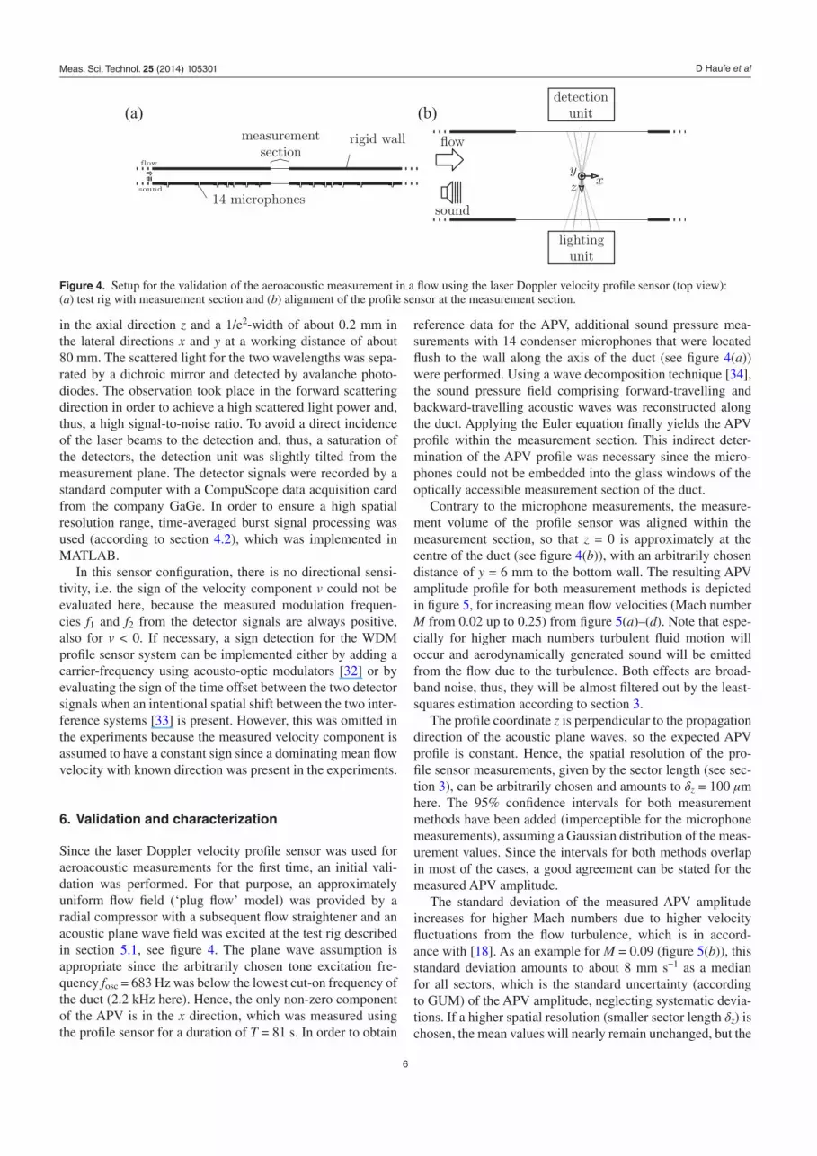
Since the laser Doppler velocity profile sensor was used for aeroacoustic measurements for the first time, an initial vali-dation was performed. For that purpose, an approximately uniform flow field (‘plug flow’ model) was provided by a radial compressor with a subsequent flow straightener and an acoustic plane wave field was excited at the test rig described in section 5.1, see figure 4. The plane wave assumption is appropriate since the arbitrarily chosen tone excitation fre-quency fosc = 683 Hz was below the lowest cut-on frequency of the duct (2.2 kHz here). Hence, the only non-zero component of the APV is in the x direction, which was measured using the profile sensor for a duration of T = 81 s. In order to obtain
reference data for the APV, additional sound pressure mea-surements with 14 condenser microphones that were located flush to the wall along the axis of the duct (see figure 4(a)) were performed. Using a wave decomposition technique [34], the sound pressure field comprising forward-travelling and backward-travelling acoustic waves was reconstructed along the duct. Applying the Euler equation finally yields the APV profile within the measurement section. This indirect deter-mination of the APV profile was necessary since the micro-phones could not be embedded into the glass windows of the optically accessible measurement section of the duct.
Contrary to the microphone measurements, the measure-ment volume of the profile sensor was aligned within the measurement section, so that z = 0 is approximately at the centre of the duct (see figure 4(b)), with an arbitrarily chosen distance of y = 6 mm to the bottom wall. The resulting APV amplitude profile for both measurement methods is depicted in figure 5, for increasing mean flow velocities (Mach number M from 0.02 up to 0.25) from figure 5(a)–(d). Note that espe-cially for higher mach numbers turbulent fluid motion will occur and aerodynamically generated sound will be emitted from the flow due to the turbulence. Both effects are broad-band noise, thus, they will be almost filtered out by the least-squares estimation according to section 3.
The profile coordinate z is perpendicular to the propagation direction of the acoustic plane waves, so the expected APV profile is constant. Hence, the spatial resolution of the pro-file sensor measurements, given by the sector length (see sec-tion 3), can be arbitrarily chosen and amounts to δz = 100 µm here. The 95% confidence intervals for both measurementmethods have been added (imperceptible for the microphone measurements), assuming a Gaussian distribution of the meas-urement values. Since the intervals for both methods overlap in most of the cases, a good agreement can be stated for the measured APV amplitude.
The standard deviation of the measured APV amplitude increases for higher Mach numbers due to higher velocity fluctuations from the flow turbulence, which is in accord-ance with [18]. As an example for M = 0.09 (figure 5(b)), this standard deviation amounts to about 8 mm s−1 as a median for all sectors, which is the standard uncertainty (according to GUM) of the APV amplitude, neglecting systematic devia-tions. If a higher spatial resolution (smaller sector length δz) is chosen, the mean values will nearly remain unchanged, but the
Figure 4. Setup for the validation of the aeroacoustic measurement in a flow using the laser Doppler velocity profile sensor (top view): (a) test rig with measurement section and (b) alignment of the profile sensor at the measurement section.
measurement
(a) (b)
section
14 microphones
rigid wall
flow
sound
flow
sound
xz
y
detectionunit
lightingunit
Meas. Sci. Technol. 25 (2014) 105301

D Haufe et al
7
standard uncertainty of the measured APV amplitude in each sector will be higher due to the smaller number Nv of velocity samples per sector, according to (5). In each case, the standard uncertainty is higher for the outer sectors in the measurement volume. This is because the frequency of particle occurrences is smaller in the outer sectors due to a smaller lateral width (see figure 2), thus, the number of velocity samples obtained in these sectors is generally less.
For the sake of completeness, it should be mentioned that both the mean flow velocity v0 and the APV phase φosc were also investigated within the validation, but are not depicted here. The measured profile of the mean flow velocity is nearly uniform and shows a good agreement with the results from reference measurements using a Prandtl probe. The profile of the measured phase is also approximately uniform, which is in accordance with the acoustic plane wave assumption. As a consequence, the validation of the profile sensor for aeroa-coustic measurements is successful.
7. Application
The first application of the laser Doppler velocity profile sensor for spatially resolved aeroacoustic measurements is described in the following. For this purpose, a generic per-forated acoustic liner with bias flow was investigated, see
figure 6. The liner perforation is based on a design from [11] and has 53 regularly arranged circular orifices with a diameter of 2.5 mm (see figure 6(a))andaporosityof6.8%.Behindthe perforation, a single resonator volume (cavity) is situated. An acoustic excitation with a tone frequency of fosc = 1073 Hz was used, where the liner has the highest damping perfor-mance (dissipation coefficient of nearly 60% [11]). Here, a grazing flow over the perforated liner with a mean velocity of about 3 m s−1 and a bias flow through the perforation with a mass flow rate of about 5 kg h−1 were used, the applied SPL was about 122 dB. The velocity component in the y direction was measured in the vicinity of the central orifice, where (x, y, z) = 0 is at the centre of that orifice, see figure 6(b). In order to span approximately the whole diameter of the orifice within one profile measurement of v(z), the length of the measure-ment volume was increased from 1.2 mm to about 2.2 mm by reducing the crossing angle between the laser beams for both fringe systems, which was accomplished using replaced lenses with a different focal length. To get a velocity field v(z, y), multiple velocity profiles were sequentially obtained with a measurement duration of T = 300 s for each profile. Between the profiles, the profile sensor was traversed in the direction of the y axis, where a minimum distance of y = 350 µm to the liner was reached. In order to enable this near-field measure-ment, both lighting unit and detection unit of the sensor were slightly tilted to the surface of the liner to avoid shadowing
Figure 5. Measured APV amplitude profile for the tone frequency fosc = 683 Hz at different flow Mach numbers M, a minimum APV amplitude of about 4 mm s−1 has been resolved: (a) M = 0.02, SPL: 99 dB and (b) M = 0.09, SPL: 121 dB and (c) M = 0.19, SPL: 125 dB and (d) M = 0.25, SPL: 126 dB.
−0.6 −0.4 −0.2 0 0.2 0.4 0.60
5
10
15
20
25
30(a) (b)
(c) (d)
lateral position z [mm]
AP
Vam
plit
ude
v osc
[mm
/s]
profile sensormicrophones
−0.6 −0.4 −0.2 0 0.2 0.4 0.60
50
100
150
200
250
300
lateral position z [mm]
AP
Vam
plit
ude
v osc
[mm
/s]
profile sensormicrophones
−0.6 −0.4 −0.2 0 0.2 0.4 0.60
50
100
150
200
250
300
lateral position z [mm]
AP
Vam
plit
ude
v osc
[mm
/s]
profile sensormicrophones
−0.6 −0.4 −0.2 0 0.2 0.4 0.60
50
100
150
200
250
300
lateral position z [mm]
AP
Vam
plit
ude
v osc
[mm
/s]
profile sensormicrophones
Meas. Sci. Technol. 25 (2014) 105301

D Haufe et al
8
effects. The tilting angle θ ≈ 4° of the lighting unit was equal to the largest of the half crossing angles of the beam pairs. As a consequence, the direction of the measured velocity compo-nent as well as the profile coordinate, which is coupled to the optical axis of the profile sensor, are also tilted by the same angle. However, this ancillary effect can be neglected here since θ is small.
The resulting fields for the measured velocity parameters vosc and φosc are depicted for a spatial resolution of δz = 100 µm in figure 7 as an arbitrarily chosen example for a plane which is eccentric to the central orifice with a distance of x = 1 mm in the downstream direction. Note that the measured param-eter fields in figure 7 show a certain asymmetry to z = 0, which results from the eccentric feeding of the bias flow into the cavity. The measured field of the mean flow velocity in figure 7(a) reveals the bias flow in y direction through the ori-fice with an average velocity of about 7 m s−1 in the vicinity of the perforation. The mean velocity of the bias flow decreases with larger distance from the perforation, as expected. The amplitude of the velocity oscillation in figure 7(b) is up to 3 m s−1, where the maximum is located near the perforation, especially at the rim of the orifice at z ≈ 0.5 mm. The velocity oscillation comprises not only the APV, but also an acousti-cally induced flow velocity oscillation, which is in accordance with e.g. [11, 18]. To separate the acoustic velocity oscillation from the acoustically induced flow oscillation, the application of the Helmholtz Hodge decomposition [35] is pursued in the
future, which requires an extension to volumetric measure-ment of three components of the velocity vector.
The standard deviation for the measured velocity oscilla-tion amplitude is about 1 mm s−1. This value is mainly given by the flow turbulence, since the measurement uncertainty without turbulence can be estimated to about 0.1 mm s−1 here (according to section 4.1). To illustrate the relation of the velocity oscillation phase within the measured field, the phase-resolved oscillation is depicted in figure 8 at four dif-ferent phases. The phase-resolved results indicate that coherent flow structures, in other words: vortices, are shed from the orifice. Those vortices are supposed to result from the sound–flow interaction, since the oscillation was not pre-sent without acoustic excitation or without flow (results not depicted here). This coincides with former theoretical works and experimental investigations e.g. in [12].
For comparison of the results with different spatial reso-lutions, the resulting mean flow velocity v0 and oscillation amplitude vosc at the tone frequency fosc = 1073 Hz were deter-mined for different sector lengths δz = 100 µm and δz = 10 µm. The results are depicted in figure 9 as an example for one pro-file at a distance of y = 1 mm to the perforation.
The results qualitatively agree for both spatial resolutions, but the uncertainties differ approximately by the factor 10 according to (5), because the number Nv of velocity samples per sector differs by a factor of 10. The results indicate that the spatial resolution of 100 µm is sufficient for the geometry
Figure 6. Arrangement of the aeroacoustic measurement at a perforated liner with bias flow using laser Doppler velocity profile sensor (a) top view showing the perforation of the liner (b) side view showing both lighting and detection optics are tilted (note that θ ≈ 4° is depicted exaggeratedly for the sake of clarity).
8.5 mm
2.5mm
grazing flow
sound
xz
y
lightingunit
detectionunit
(a)
detectionunit
z
y
xθ
lightingunit
biasflow
(b)
Figure 7. Measured fields of the velocity parameters (y component) with a spatial resolution of δz = 100 µm at x = 1 mm for the tone frequency fosc = 1073 Hz: (a) mean flow velocity and (b) velocity oscillation amplitude.
lateral position z [mm]
liner
dist
ance
y[m
m]
−0.500.51
0
0.5
1
1.5
2
2.5
3(a) (b)
mea
nflo
wve
loci
tyv 0
[m/s
]
0
2
4
6
8
10
lateral position z [mm]
liner
dist
ance
y[m
m]
−0.500.51
0
0.5
1
1.5
2
2.5
3
osci
llati
onam
plit
ude
v osc
[m/s
]
0
0.5
1
1.5
2
2.5
3
Meas. Sci. Technol. 25 (2014) 105301

D Haufe et al
9
parameters of the investigated orifice here. Notwithstanding, it is shown that the aeroacoustic measurement with microscale reso-lution is possible with the profile sensor. Future application of the sensor will be measurements within the dissipation range, where the smallest flow structures having the size of the Kolmogorov length scale (here roughly 20 µm) are assumed, according to [36, p 187]. Furthermore, the sensor offers perspectives for aeroa-coustic investigations of e.g. micro-perforated liners [37].
8. Summary and outlook
The near-field measurement of aeroacoustic fields with high spatial resolution by means of a laser Doppler velocity profile sensor was presented. At first, a successful validation of the acoustic particle velocity (APV) measurement in a flow duct with a maximum Mach number of 0.25 was demonstrated using reference measurements with an established microphone tech-nique. It was shown that the uncertainty of the measured APV amplitude mainly depends on the mean velocity of the super-imposed flow, which coincides with higher turbulent velocity fluctuations. For instance, the standard uncertainty for the APV amplitude amounts to 8 mm s−1 at a mean flow velocity of about
30 m s−1 (corresponding to Mach 0.09), assuming a measure-ment duration of 81 s and a spatial resolution of 100 µm.
The profile sensor was applied for aeroacoustic measure-ments at a perforated liner with bias flow and grazing flow for the first time. In addition to the mean flow velocity, acoustically induced flow velocity oscillations at the acoustic excitation frequency were resolved in the vicinity of the central orifice, with an all-time high spatial resolution of 10 µm. The spatially resolved amplitude of this velocity oscillation revealed that the oscillation is maximum at the rim of the orifice, the amplitude amounts to about 3 m s−1 there. The measured field of the phase-resolved oscillation indicates vortex shedding from the perfora-tion. Consequently, it is assumed that the sound–flow interaction initiates a transfer from acoustic energy to flow energy at this bias flow liner configuration. In order to prove this assump-tion and, furthermore, to locate and quantify the energy transi-tion, an energy balance is needed in the future. This requires a separation of the acoustically induced velocity oscillation from the acoustic particle velocity. For this purpose, the Helmholtz Hodge decomposition is aspired in future investigations, which necessitates a sensor extension for three-dimensional, three-component measurements. As a result of the microscale resolu-tion, the sensor is a valuable measurement tool for aeroacoustic
Figure 8. Phase-resolved velocity oscillation (y component) with a spatial resolution of δz = 100 µm at x = 1 mm for the tone frequency fosc = 1073 Hz: (a) phase 0 (b) phase π/2 (c) phase π and (d) phase 3 π/2.
liner
dist
ance
y[m
m]
lateral position z [mm]−0.500.51
0
1
2
3(a) (b) (c) (d)
lateral position z [mm]−0.500.51
lateral position z [mm]−0.500.51
lateral position z [mm]−0.500.51
velo
city
osci
llati
on[m
/s]
−3
−2
−1
0
1
2
3
Figure 9. Measured profile of the velocity parameters (y component) for different spatial resolutions δz at x = 1 mm and a distance of y = 1 mm to the surface of the liner: (a) mean flow velocity and (b) velocity oscillation amplitude.
(a) (b)
−0.500.51
0
2
4
6
8
10
lateral position z [mm]
mea
nflo
wve
loci
tyv 0
[m/s
]
δz = 100 µm
δz = 10 µm
−0.500.51
0
0.5
1
1.5
2
2.5
3
lateral position z [mm]
osci
llati
onam
plit
ude
v osc
[m/s
]
δz = 100 µm
δz = 10 µm
Meas. Sci. Technol. 25 (2014) 105301

D Haufe et al
10
investigations, especially for near-field measurements at e.g. micro-perforated liners or thermo-acoustic refrigerators.
Acknowledgments
We thank the German Research Foundation (DFG) for the funding of the projects CZ 55/25-1 and EN 797/2-1. Sincere thanks are given to ILA GmbH that provided the particle gen-erator PIVpart40. The authors are indebted to André Fischer for supporting the measurements. Jörg König is thanked for fruitful discussions.
Appendix A. Systematic deviation for time-averaged burst estimation
The signal processing employing the time-averaged frequency estimation (see section 3) yields time-averaged modula-tion frequencies ∀ =f t k( ) 1, 2k for each burst at its central burst time t . If the modulation frequencies are not constant within the burst duration, there will be a difference between f t( )k which is averaged over the burst duration Tburst and the actual modulation frequencies f t( )k . Consequently, the average velocity v t( ) will differ from the actual velocity v t( ). Eventually, a systematic deviation for the measured APV amplitude results, which is explained in the following.
At first, a single burst of a particle with constant position z is assumed. According to (1), the modulation frequencies
=f t v t d z( ) ( )/ ( )k k (A.1)
are time-dependent since they are proportional to the time-dependent velocity signal
ω φ
ω φ ω
= + +
= − + + +
φ′ ′
v t v t v
v t t t v
( ) cos ( )
cos ( ( ) )
t
osc osc osc 0
osc osc osc osc 0
osc
(A.2)
from (3). Notwithstanding, the term 2π fosc = ωosc has been replaced. Furthermore, the random term vturb(t) in (3) has been removed, since it vanishes in case of averaging and, thus, does not cause any systematic deviation to be considered here. Moreover, the time variable t′ is introduced in (A.2) to facili-tate the calculation of the average velocity
⎜ ⎟
⎡⎣⎢ ⎛
⎝⎞⎠
⎤⎦⎥
ω φ
π φ
=
=∫ ′ ′
∫ ′ ′ ′
=∫ ′ ′
∫ ′ + ′ ′ +
= … ≈ − ′ +
ω φ ω φ
−
+−
+
−
+−
+
′ ′ − ′ ′
( )
v t d z f t
d z
w t t
f t w t t
w t t
v t w t t v
f T v v
( ) ( )· ( )
( )·1
( )d
( ) ( )d
1
( )d
· cos · ( )d
exp4
cos
k k
k
T
TT
T
k
T
TT
T
t t
v
/2
/2/2
/2
/2
/2/2
/2
osc osc osc
cos( )cos( ) sin( )sin( )
0
osc burst
2
osc osc 0
burst
burstburst
burst
burst
burstburst
burst
osc osc osc osc
osc
(A.3)
from a single burst with the central time t, using (A.1) and (A.2). To ensure an efficient estimation of the average frequency fk in (A.3), a weighting function w(t′) = (exp{−2[2t′/Tburst]2})2 was
chosen such that the estimation is efficient, assuming signal-independent noise [26]. Here, w(t′) represents the squared magnitude of the Gaussian envelope of a burst signal and Tburst denotes its temporal 1/e2 width. The integral in (A.3) has been solved as an approximation for the interval (−∞, + ∞), which is appropriate since the integrand strongly attenuates beyond the integration limits ± Tburst/2.
Obviously, the averaged velocity from (A.3) is different from the actual velocity
φ= ′ +v t v v( ) cos ,osc osc 0 (A.4)
so that the estimated APV amplitude vosc in (A.3) exhibits a relative deviation
⎜ ⎟⎡⎣⎢
⎛⎝
⎞⎠
⎤⎦⎥Δ π= − = − −v
v
v v
vf Texp
41.osc
osc
osc osc
oscosc burst
2
(A.5)
Considering the sensor setup from section 5.2, this system-aticrelativedeviationfortheAPVamplitudeisbelow1%(forfosc < 2 kHz and v0 > 3 m s−1) and can be corrected for a given acoustic frequency and known burst duration. Note that no deviation results for the phase of the APV from this averaging effect.
Appendix B. Uncertainty of the measured velocity due to frequency uncertainty
According to section 2, the measured velocity v equals
= · ∀ =v f d z q f f k( ( ( , ))) 1, 2,k k 1 2 (B.1)
using the estimated modulation frequency fk and the estimated fringe spacing dk(z), both from the kth fringe system. Note that dk is essentially evaluated using both f1 and f2.
Assuming uncorrelated frequency estimations with the uncertainties σf1 and σf2 (systematic deviations exluded), the resulting relative uncertainty of the velocity reads
⎛
⎝⎜
⎞
⎠⎟
⎛
⎝⎜
⎞
⎠⎟
⎛
⎝⎜
⎞
⎠⎟
⎛
⎝⎜
⎞
⎠⎟
σ σ σ
σ σ
= ∂∂
+ ∂∂
= ∂∂
· · + ∂∂
· ·
v v
v
f
v
f
v
f d f
v
f d f
1
1 1,
v
1f
2
2f
2
1 1
f
1
2
2 2
f
2
2
1 2
1 2
(B.2)
applying the Gaussian uncertainty propagation to (B.1). The partial derivatives in (B.2) can be obtained from (B.1), which is presented using k = 1 only in the following (the final result will be the same for k = 2):
∂∂
= +∂
∂∂∂
=∂
∂
v
fd f f f
d f f
f
v
ff
d f f
f
( , )( , )
and
( , ),
11 1 2 1
1 1 2
1
21
1 1 2
2
(B.3)
where
∂∂
= ∂∂
· ∂∂
· ∂∂
∀ =d f f
f
d z
z
z q
q
q
fk
( , ) ( ) ( )1, 2
k k
1 1 2 1 (B.4)
Meas. Sci. Technol. 25 (2014) 105301

D Haufe et al
11
holds. Using
⎧⎨⎩
⎫⎬⎭
⎧⎨⎪
⎩⎪
⎫⎬⎪
⎭⎪
⎧⎨⎩
⎫⎬⎭
∂∂
· ∂∂
= ′ · ∂∂
= ′ ·∂
∂
= ′ · ′ · − · ′ =+
−−
−
( )d z
z
z q
qd z
q z
zd z
z
d zd z d d d z
d
d
q z r z
( ) ( )( )
( )( )
( )( ) ( )
1 ( ) ( ),
d z
d z11
1
1
( )
( )
1
11 2 1 2
22
12
1
2
(B.5)
where = − ′′
r zd z
d z( )
( )
( )2
1 is the negative ratio of the slopes of the
fringe spacings, as well as
∂∂
= − ∂∂
=q
fq f
q
ff/ , 1/
11
21 (B.6)
obtained from (2), and successive inserting into (B.2) yields
⎛
⎝⎜
⎞
⎠⎟
⎛
⎝⎜
⎞
⎠⎟σ σ σ
=+
· ++
·v
qr
qr f qr f1
1
1.
f fv
1
2
2
21 2 (B.7)
For a typical sensor setup, the fringe spacings d1 and d2 are nearly equal, i.e. q ≈ 1. Moreover, the slopes d′1(z) and d′2(z) nearly have the same absolute value, but opposite signs, i.e. r ≈ 1. Furthermore, the relative frequency uncertainties σ f/f kk
have approximately the same value σf/f for k = 1, 2. Hence, (B.7) can be simplified to
σ σ≈
v f
1
2.
fv (B.8)
This expression for the velocity uncertainty is different from the one previously stated in [23] and related publica-tions, where the correlation between dk(z) and fk has been ignored.
References
[1] Huelsz G, López-Alquicira F and Ramos E 2002 Velocity measurements in the oscillatory boundary layer produced by acoustic waves Exp. Fluids 32 612–5
[2] Castrejón-Pita J R, Castrejón-Pita A A, Huelsz G and Tovar R 2006 Experimental demonstration of the Rayleigh acoustic viscous boundary layer theory Phys. Rev. E 73 036601
[3] Campbell M, Cosgrove J A, Greated C A, Jack S and Rockliff D 2000 Review of LDA and PIV applied to the measurement of sound and acoustic streaming Opt. Laser Technol. 32 629–39
[4] Nabavi M, Kamran Siddiqui M H and Dargahi J 2007 Simultaneous measurement of acoustic and streaming velocities using synchronized PIV technique Meas. Sci. Technol. 18 1811–7
[5] Berson A, Michard M and Blanc-Benon P 2008 Measurement of acoustic velocity in the stack of a thermoacoustic refrigerator using particle image velocimetry Heat Mass Transfer 44 1015–23
[6] Mao X and Jaworski A J 2010 Application of particle image velocimetry measurement techniques to study turbulence characteristics of oscillatory flows around parallel-plate structures in thermoacoustic devices Meas. Sci. Technol. 21 035403
[7] Morley E, Steinmann T, Casas J and Robert D 2012 Directional cues in Drosophila melanogaster audition:
structure of acoustic flow and inter-antennal velocity differences J. Exp. Biol. 215 2405–13
[8] Breakey D E S, Fitzpatrick J A and Meskell C 2013 Aeroacoustic source analysis using time-resolved PIV in a free jet Exp. Fluids 54 1–6
[9] Bailliet H, Boucheron R, Dalmont J P, Herzog P, Moreau S and Valière J C 2012 Setting up an experimental apparatus for the study of multimodal acoustic propagation with turbulent mean flow Appl. Acoust. 73 191–7
[10] Eldredge J D and Dowling A P 2003 The absorption of axial acoustic waves by a perforated liner with bias flow J. Fluid Mech. 485 307–35
[11] Heuwinkel C, Fischer A, Röhle I, Enghardt L, Bake F, Piot E and Micheli F 2010 Characterization of a perforated liner by acoustic and optical measurements 16th AIAA/CEAS Aeroacoustics Conf. (Stockholm, Sweden, 7–9 June 2010) pp 2010–65
[12] Rupp J, Carrotte J and Spencer A 2010 Interaction between the acoustic pressure fluctuations and the unsteady flow field through circular holes J. Eng. Gas Turb. Power 132 061501
[13] Zhong Z and Zhao D 2012 Time-domain characterization of the acoustic damping of a perforated liner with bias flow J. Acoust. Soc. Am. 132 271–81
[14] Jing X and Sun X 1999 Experimental investigations of perforated liners with bias flow J. Acoust. Soc. Am. 106 2436–41
[15] Minotti A, Simon F and Gantié F 2008 Characterization of an acoustic liner by means of laser Doppler velocimetry in a subsonic flow Aerospace Sci. Technol. 12 398–407
[16] de Bree H E 2003 An overview of microflown technologies Acta Acust. United Ac. 89 163–72
[17] Hann D B and Greated C A 1997 The measurement of flow velocity and acoustic particle velocity using particle-image velocimetry Meas. Sci. Technol. 8 1517–22
[18] Haufe D, Fischer A, Czarske J, Schulz A, Bake F and Enghardt L 2013 Multi-scale measurement of acoustic particle velocity and flow velocity for liner investigations Exp. Fluids 54 1–7
[19] Taylor K J 1976 Absolute measurement of acoustic particle velocity J. Acoust. Soc. Am. 59 691–4
[20] Hann D and Greated C 1999 The measurement of sound fields using laser Doppler anemometry Acta Acust. United Ac. 85 401–11
[21] Thompson M W and Atchley A A 2005 Simultaneous measurement of acoustic and streaming velocities in a standing wave using laser Doppler anemometry J. Acoust. Soc. Am. 117 1828–38
[22] Miles P C 1996 Geometry of the fringe field formed in the intersection of two Gaussian beams Appl. Opt. 35 5887–95
[23] Czarske J, Büttner L, Razik T and Müller H 2002 Boundary layer velocity measurements by a laser Doppler profile sensor with micrometre spatial resolution Meas. Sci. Technol. 13 1979–89
[24] Albrecht H E, Borys M, Damaschke N and Tropea C 2003 Laser Doppler and Phase Doppler Measurement Techniques (New York: Springer)
[25] Neumann M, Shirai K, Büttner L and Czarske J 2012 A novel laser doppler array sensor for measurements of micro-scale velocity correlations in turbulent flows Flow Meas. Instrum. 28 7–15
[26] Czarske J W 2001 Statistical frequency measuring error of the quadrature demodulation technique for noisy single-tone pulse signals Meas. Sci. Technol. 12 597–614
[27] Simon L, Richoux O, Degroot A and Lionet L 2008 Laser Doppler velocimetry for joint measurements of acoustic and mean flow velocities: LMS-based algorithm and CRB calculation IEEE Trans. Instrum. Meas. 57 1455–64
[28] ISO 1993 Guide to the expression of uncertainty in measurement Technical Report ISO/IEC Guide 98-3 : 2008 (Geneva: International Organization for Standardization)
Meas. Sci. Technol. 25 (2014) 105301

D Haufe et al
12
[29] Haufe D, Schlüßler R, Fischer A, Büttner L and Czarske J 2012 Optical multi-point measurement of the acoustic particle velocity in a superposed flow using a spectroscopic laser technique Meas. Sci. Technol. 23 085306
[30] Büttner L, Skupsch C, König J and Czarske J 2010 Optic simulation and optimization of a laser Doppler velocity profile sensor for microfluidic applications Opt. Eng. 49 073602
[31] Raffel M, Willert C, Werely S and Kompenhans J 1998 Particle Image Velocimetry: A Practical Guide (New York: Springer)
[32] Shirai K, Büttner L, Czarske J, Müller H and Durst F 2005 Heterodyne laser-Doppler line-sensor for highly resolved velocity measurements of shear flows Flow Meas. Instrum. 16 221–8
[33] König J, Mühlenhoff S, Eckert K, Büttner L, Odenbach S and Czarske J 2011 Velocity measurements inside the
concentration boundary layer during copper-magneto-electrolysis using a novel laser Doppler profile sensor Electrochim. Acta 56 6150–6
[34] Lahiri C, Enghardt L, Bake F, Sadig S and Gerendás M 2011 Establishment of a high quality database for the acoustic modeling of perforated liners J. Eng. Gas Turb. Power 133 091503
[35] De Roeck W, Baelmans M and Desmet W 2007 An aerodynamic/acoustic splitting technique for hybrid CAA applications 15th AIAA/CEAS Aeroacoustics Conf. (Rome, Italy, 21–23 May 2007) pp 2007–26
[36] Pope S B 2000 Turbulent Flows (Cambridge: Cambridge University Press)
[37] Tayong R B, Dupont T and Leclaire P 2013 Sound absorption of a micro-perforated plate backed by a porous material under high sound excitation: measurement and prediction Int. J. Eng. Technol. 2 281–92
Meas. Sci. Technol. 25 (2014) 105301


