Embed Size (px)
Citation preview
applied sciences
Article
Aerodynamic Simulation of Helicopter Based onPolyhedron Nested Grid Technology
Chenglong Zhou * and Ming Chen
School of Aeronautic Science and Engineering, Beihang University, Xueyuan Road No.37, Beijing 100191, China;[email protected]* Correspondence: [email protected]; Tel.: +86-1851-527-9185
Received: 5 November 2020; Accepted: 20 November 2020; Published: 23 November 2020
Abstract: In this paper, a computational fluid dynamics (CFD) simulation method based on thepolyhedral nested grid is developed. By comparing the simulation and test results of the hovering flowfield of the Caradonna–Tung rotor, the forward flight flow field of the AH-1G rotor, the interferenceflow field of the Robin rotor/fuselage, and the hovering and forward flight flow field of a coaxialrotor, it is proven that the method proposed in this paper can achieve high calculation accuracy undervarious working conditions. The dual time-stepping method is used for the transient simulation,and the Spalart–Allmaras (S-A) turbulence model, which is widely used in aviation, is adopted inthe simulation.
Keywords: interference flow field; blade; coaxial rotor; polyhedron nested grid; cyclic pitch
1. Introduction
Experimental methods and computational fluid dynamics (CFD) simulation are the mainapproaches to study the aerodynamic characteristics of helicopters. The experimental approachis more convincing, and sometimes more effective, for classic problems such as airframe dragreduction [1,2]. However, the experimental method has the disadvantages of long period and highinvestment. Meanwhile, the spatial resolution of the experimental method is low, so the detailedfeatures inside the flow field are difficult to observe. Currently, with the improvement of CFDtechnology, its features of intelligence, convenience, and high precision are increasingly prominent.CFD has become an important method in the aerodynamic performance research of helicopters.
At present, CFD technology has made great contributions to aerodynamic calculation ofhelicopters [3,4]. In particular, the overlapping grid method [5] has attracted much attention inthis field because of its unique advantages. It is suitable for almost all flight conditions of a variety ofhelicopters, and is currently one of the most widely used methods in this field. In addition, the slidingmesh method is often applied to helicopter hovering. It was proposed and validated by Steijl et al. [6].For rotor CFD/CSD coupling simulation, various deformation mesh methods have been widely used,among which the spring mesh method is the most famous. Bottasso et al. [7] improved the spring meshmethod and solved its shortcoming of easily forming grid deformities, so that it could deal with theproblem of large deformation movement. The adaptive mesh method is widely applied in capturingthe wake of the rotor vortex. This method usually uses a Cartesian grid as the background grid toadapt the background mesh conveniently. The famous American Helios project [8,9] successfullyapplied the adaptive mesh method to the rotor vortex wake capture and achieved remarkable effect.Jameson and Mavriplis [10] greatly improved the convergence speed of the simulation through themultigrid technology. Li et al. [11] developed a method to generate coarse grids of multiple grids,which can greatly reduce the convergence time of simulation. Nishikawa and Diskin [12] addedmultigrid technology to the structured overset mesh of the rotor, and the result shows that the multigrid
Appl. Sci. 2020, 10, 8304; doi:10.3390/app10228304 www.mdpi.com/journal/applsci
Appl. Sci. 2020, 10, 8304 2 of 21
using a structured grid can better guarantee the quality of the coarse grid, thereby improving thecalculation accuracy. Shi et al. [13] developed a coupled simulation technique combining viscouswake model (VWM), computational fluid dynamics (CFD), and computational structural dynamics(CSD) to predict unsteady aerodynamic loads of rotors. Zhao et al. [14] established the CLORNS code,a robust unsteady rotor solver, to perform the transient simulation of the helicopter flow field, and theresults show that the code has high accuracy in calculating aerodynamic loads of helicopter rotors.Zhou et al. [15] developed a CFD trimming method of helicopters in forward flight and achieved agood trim effect. Barakos et al. [16] proposed an unsteady actuator disk method based on surfacecirculation distribution, and used it to simulate the flow field of rotors in hover and forward flightstates. The results show that this method is effective in capturing the major vortex structures aroundthe disk. Tang et al. [17] proposed a method based on CFD simulation to predict the airborne spraydrift and settlement under complex conditions, and applied it to the research on the downwash flowfield and droplets movement law of unmanned agricultural helicopters.
As one of the fastest developing mesh technologies in recent years, polyhedral mesh technologyhas the advantages of fewer meshes, faster convergence speed, and higher calculation accuracy.Therefore, its application in engineering is increasingly widespread. However, there is little researchon the application of this technology in helicopter flow field simulation, and the relevant literatureavailable for reference is scarce. In this paper, polyhedral mesh technology is adopted to calculate theaerodynamic characteristics of single-rotor and coaxial-rotor helicopters under hover and forwardflying conditions.
In order to prove the reliability of the simulation results, the numerical results obtained by the CFDmethod must be compared with the test data. Therefore, the relevant parameters of the simulation mustbe the same as the corresponding test conditions, including blade model, rotation speed, total distance,and so forth. Fortunately, some well-known rotor test reports provide scientists with detailed data andconfigurations for further study. In particular, the National Aeronautics and Space Administration(NASA) has made great contributions in this field.
2. CFD Simulation Method
2.1. Governing Equation and Solution Method
CFD simulation examples in this paper are all based on the Reynolds average Navier–Stokes (N-S)equation in the conservation form, as shown in Equation (1):
∂∂t
y
V
→
WdV +x
S
(→
F c −→
Fv
)·→ndS = 0 (1)
where,→
W = [ρ,ρu,ρv,ρw,ρe]T is the conservation variable,→
F c = ( f , g, h) is the convection flux,
and→
Fv = (a, b, c) is the viscous flux. These parameters can be expressed as:
f =
ρu
ρu2 + pρuvρuw
ρue + up
, g =
ρvρuv
ρv2 + pρvw
ρve + vp
, h =
ρwρuwρvw
ρw2 + pρwe + wp
(2)
a =
0τxx
τyx
τzx
uτxx + vτyx + wτzx − qx
, b =
0τxy
τyy
τzy
uτxy + vτyy + wτzy − qy
, c =
0τxz
τyz
τzz
uτxz + vτyz + wτzz − qz
(3)
Appl. Sci. 2020, 10, 8304 3 of 21
In the viscous flux, the stress can be expressed as:
τxx = 23µ
(2∂µ∂x −
∂υ∂y −
∂w∂z
), τxy = τyx = µ
(∂υ∂x + ∂u
∂y
), qx = −K∂T
∂x
τyy = 23µ
(2 ∂v∂y −
∂u∂x −
∂w∂z
), τyz = τzy = µ
(∂w∂y + ∂v
∂z
), qy = −K∂T
∂y
τzz = 23µ
(2∂w∂z −
∂u∂x −
∂v∂y
), τxz = τzx = µ
(∂w∂x + ∂u
∂z
), qz = −K∂T
∂z
(4)
By introducing the relationship between pressure and temperature, the closed equations can beobtained:
p = ρ(γ− 1)[e−
12
(u2 + v2 + w2
)](5)
p = ρRT (6)
Among them, ρ represents the density of air, p represents the pressure, e represents the total energyper unit mass of the gas, µ represents the viscosity coefficient, K represents the thermal conductivitycoefficient, T represents the temperature, qx, qy, and qz represent the components of the heat flow alongthree directions, γ represents the specific heat capacity, for ideal gas, γ = 1.4, R = 287.3.
The Spalart–Allmaras (S-A) turbulence model [18] is adopted in the simulation of this paper.This model is a single-equation turbulence model, which does not derive the precise transport equationof the vortex-viscosity coefficient, but a simplified equation obtained by referring to experimental data.Thanks to Spalart’s convenience in aviation calculation, rich experience, and large amount of test data,the S-A model has been widely applied in aviation, especially in shock wave capture.
Different interpolation schemes are formed because of different discrete strategies for inviscid fluxon the interface of grid cells. The Roe format [19] of flux difference splitting (FDS) in the third-orderupwind format is adopted in this paper. This format has strong shock capture capability and is amethod to calculate inviscid flux by approximating the Riemann solution. Due to the possibility ofnonphysical understanding in the approximate Riemann solution, the entropy modified theory [20] isadopted to modify the eigenvalues in the Roe scheme.
The time discretization of the flow governing equations is based on the dual time-steppingmethod. Jameson [21] explained the method in detail. In this paper, the rotation of the foreground gridcontaining the blades is solved at 3 per time step, and each time step has 20 subiterations. It is foundthat the flow becomes quasi-stable after about 1.5 turns of rotation. Therefore, in order to shorten thecalculation time, about three rotation cycles are calculated for each working condition.
The far field boundary adopts the nonreflective boundary condition. The nonreflective boundaryis defined by Riemann invariants R+ and R−) [22]. The blade surface adopts the type of wallwithout sliding.
2.2. Grid System
In this paper, the polyhedron nested grid method is used to simulate the unsteady flow fieldof the helicopter. In this method, the flow field is usually divided into several regions, and eachregion is meshed separately. These mesh regions can overlap, nest, or overlay each other. In thisway, the difficulty of mesh generation is reduced. The key technology is to build the connectionrelationship between the mesh regions by “hole mapping”. When it comes to the fluid problem of thebody moving with time, there is also relative motion among corresponding grid blocks, so the nestedgrid method should be used at each time step respectively to build the relation between different meshregions, which can be used to transport the messages at the interface needed for the CFD simulation.There are three steps to implement the overset mesh method: hole mapping, contributing cell search,and interpolation. It should be noted that in the process of generating overlapped grids, in order toensure the interpolation accuracy at the interface of grid blocks, sufficient overlap, almost equal meshsize, and low inclination must be ensured. At the same time, the interface of the grid blocks must avoidthe large physical gradient area in the flow field.
Appl. Sci. 2020, 10, 8304 4 of 21
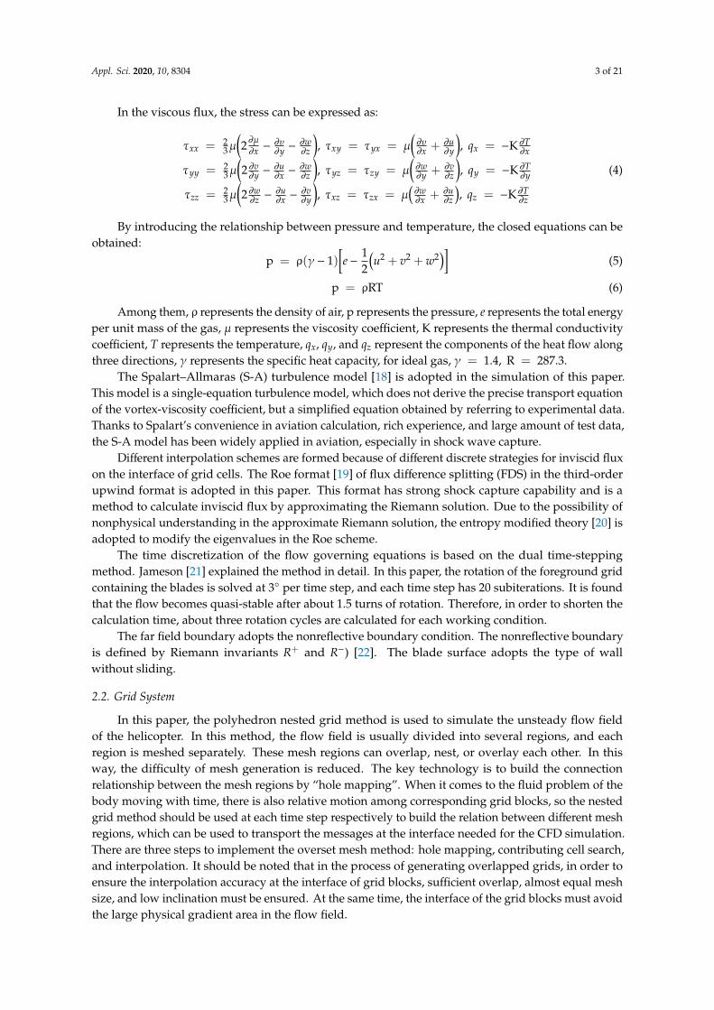
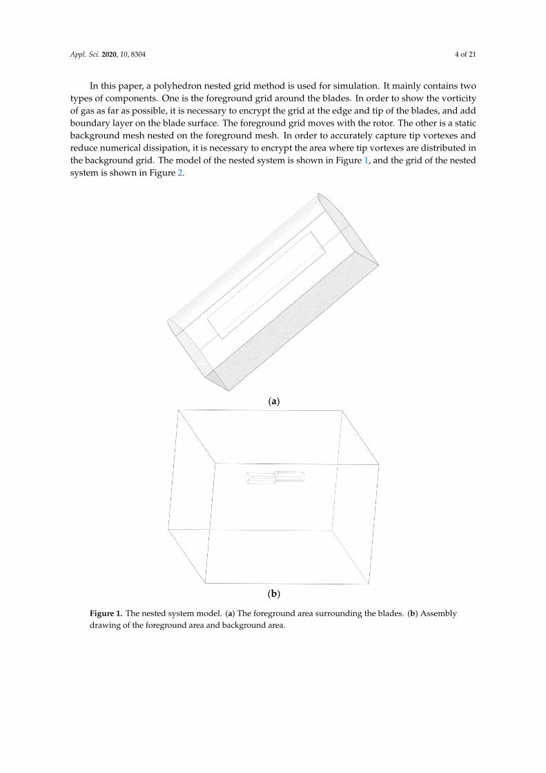
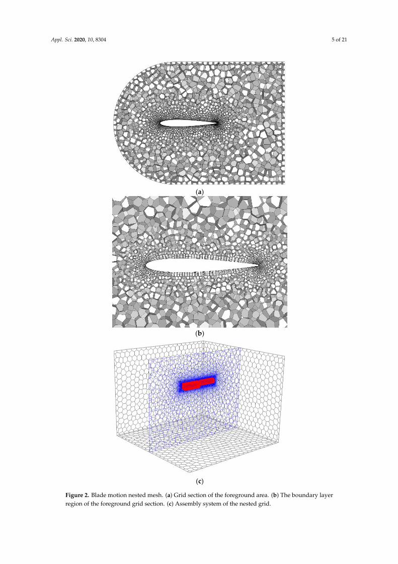
In this paper, a polyhedron nested grid method is used for simulation. It mainly contains twotypes of components. One is the foreground grid around the blades. In order to show the vorticityof gas as far as possible, it is necessary to encrypt the grid at the edge and tip of the blades, and addboundary layer on the blade surface. The foreground grid moves with the rotor. The other is a staticbackground mesh nested on the foreground mesh. In order to accurately capture tip vortexes andreduce numerical dissipation, it is necessary to encrypt the area where tip vortexes are distributed inthe background grid. The model of the nested system is shown in Figure 1, and the grid of the nestedsystem is shown in Figure 2.
Appl. Sci. 2020, 10, x FOR PEER REVIEW 4 of 22
Appl. Sci. 2020, 10, x; doi: FOR PEER REVIEW www.mdpi.com/journal/applsci
mesh method: hole mapping, contributing cell search, and interpolation. It should be noted
that in the process of generating overlapped grids, in order to ensure the interpolation accuracy
at the interface of grid blocks, sufficient overlap, almost equal mesh size, and low inclination
must be ensured. At the same time, the interface of the grid blocks must avoid the large physical
gradient area in the flow field.
In this paper, a polyhedron nested grid method is used for simulation. It mainly contains
two types of components. One is the foreground grid around the blades. In order to show the
vorticity of gas as far as possible, it is necessary to encrypt the grid at the edge and tip of the
blades, and add boundary layer on the blade surface. The foreground grid moves with the
rotor. The other is a static background mesh nested on the foreground mesh. In order to
accurately capture tip vortexes and reduce numerical dissipation, it is necessary to encrypt the
area where tip vortexes are distributed in the background grid. The model of the nested system
is shown in Figure 1, and the grid of the nested system is shown in Figure 2.
(a)
(b)
Figure 1. The nested system model. (a) The foreground area surrounding the blades. (b)
Assembly drawing of the foreground area and background area.
Figure 1. The nested system model. (a) The foreground area surrounding the blades. (b) Assemblydrawing of the foreground area and background area.
Appl. Sci. 2020, 10, 8304 5 of 21Appl. Sci. 2020, 10, x FOR PEER REVIEW 5 of 22
Appl. Sci. 2020, 10, x; doi: FOR PEER REVIEW www.mdpi.com/journal/applsci
(a)
(b)
(c)
Figure 2. Blade motion nested mesh. (a) Grid section of the foreground area. (b) The boundary
layer region of the foreground grid section. (c) Assembly system of the nested grid.
In order to verify the simulation technique proposed in this paper, numerical simulations
are carried out on the hovering condition of the Caradona–Tung (C-T) rotor, the forward flight
condition of the AH-1G rotor, the rotor/fuselage interaction flow field of Robin, and the hover
Figure 2. Blade motion nested mesh. (a) Grid section of the foreground area. (b) The boundary layerregion of the foreground grid section. (c) Assembly system of the nested grid.
Appl. Sci. 2020, 10, 8304 6 of 21
In order to verify the simulation technique proposed in this paper, numerical simulations arecarried out on the hovering condition of the Caradona–Tung (C-T) rotor, the forward flight conditionof the AH-1G rotor, the rotor/fuselage interaction flow field of Robin, and the hover and forward flightconditions of coaxial rotor. In addition, the calculated results are compared with the test data.
3. Validation of CFD Simulation Method
3.1. C-T Rotor in Hover
In this section, the test model of the C-T rotor [23] is taken as an example to verify the accuracy ofnumerical simulation in the hovering state. The detailed parameters of the C-T rotor are shown inTable 1.
Table 1. Detailed parameters of C-T rotor.
Number of Blades 2
Blade radius R 1.143 mPlane shape of blade Rectangle
Airfoil NACA0012Chord length c 0.1905 mUndercut Rcut 0.243 RTorsion angle 0
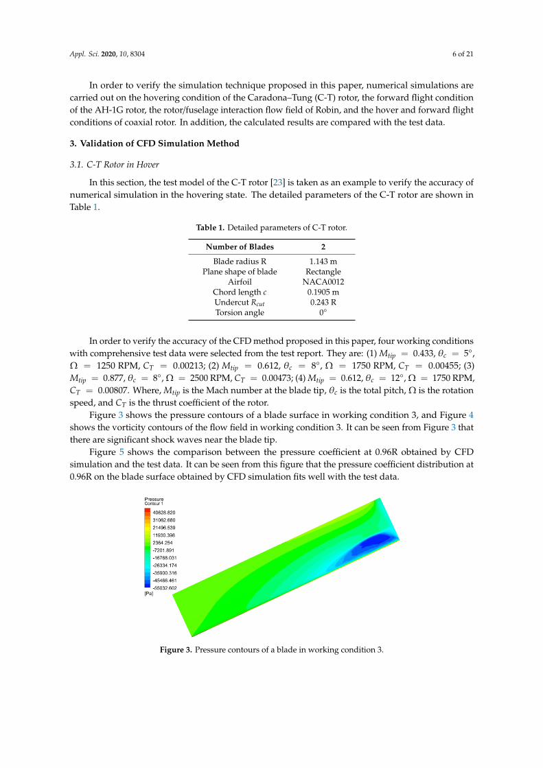
In order to verify the accuracy of the CFD method proposed in this paper, four working conditionswith comprehensive test data were selected from the test report. They are: (1) Mtip = 0.433, θc = 5,Ω = 1250 RPM, CT = 0.00213; (2) Mtip = 0.612, θc = 8, Ω = 1750 RPM, CT = 0.00455; (3)Mtip = 0.877, θc = 8, Ω = 2500 RPM, CT = 0.00473; (4) Mtip = 0.612, θc = 12, Ω = 1750 RPM,CT = 0.00807. Where, Mtip is the Mach number at the blade tip, θc is the total pitch, Ω is the rotationspeed, and CT is the thrust coefficient of the rotor.
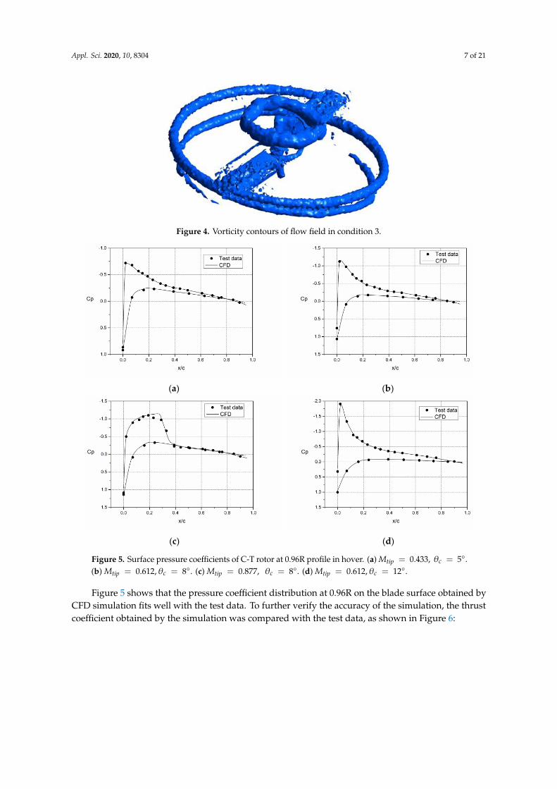
Figure 3 shows the pressure contours of a blade surface in working condition 3, and Figure 4shows the vorticity contours of the flow field in working condition 3. It can be seen from Figure 3 thatthere are significant shock waves near the blade tip.
Figure 5 shows the comparison between the pressure coefficient at 0.96R obtained by CFDsimulation and the test data. It can be seen from this figure that the pressure coefficient distribution at0.96R on the blade surface obtained by CFD simulation fits well with the test data.
Appl. Sci. 2020, 10, x FOR PEER REVIEW 7 of 22
Appl. Sci. 2020, 10, x; doi: FOR PEER REVIEW www.mdpi.com/journal/applsci
Figure 3. Pressure contours of a blade in working condition 3.
Figure 4. Vorticity contours of flow field in condition 3.
Figure 5 shows the comparison between the pressure coefficient at 0.96R obtained by CFD
simulation and the test data. It can be seen from this figure that the pressure coefficient
distribution at 0.96R on the blade surface obtained by CFD simulation fits well with the test
data.
(a) (b)
Figure 3. Pressure contours of a blade in working condition 3.
Appl. Sci. 2020, 10, 8304 7 of 21
Appl. Sci. 2020, 10, x FOR PEER REVIEW 7 of 22
Appl. Sci. 2020, 10, x; doi: FOR PEER REVIEW www.mdpi.com/journal/applsci
Figure 3. Pressure contours of a blade in working condition 3.
Figure 4. Vorticity contours of flow field in condition 3.
Figure 5 shows the comparison between the pressure coefficient at 0.96R obtained by CFD
simulation and the test data. It can be seen from this figure that the pressure coefficient
distribution at 0.96R on the blade surface obtained by CFD simulation fits well with the test
data.
(a) (b)
Figure 4. Vorticity contours of flow field in condition 3.
Appl. Sci. 2020, 10, x FOR PEER REVIEW 7 of 22
Appl. Sci. 2020, 10, x; doi: FOR PEER REVIEW www.mdpi.com/journal/applsci
Figure 3. Pressure contours of a blade in working condition 3.
Figure 4. Vorticity contours of flow field in condition 3.
Figure 5 shows the comparison between the pressure coefficient at 0.96R obtained by CFD
simulation and the test data. It can be seen from this figure that the pressure coefficient
distribution at 0.96R on the blade surface obtained by CFD simulation fits well with the test
data.
(a) (b)
Appl. Sci. 2020, 10, x FOR PEER REVIEW 8 of 22
Appl. Sci. 2020, 10, x; doi: FOR PEER REVIEW www.mdpi.com/journal/applsci
(c) (d)
Figure 5. Surface pressure coefficients of C-T rotor at 0.96R profile in hover. (a) 𝑀𝑡𝑖𝑝 =
0.433, 𝜃𝑐 = 5° . (b) 𝑀𝑡𝑖𝑝 = 0.612, 𝜃𝑐 = 8°. (c) 𝑀𝑡𝑖𝑝 = 0.877, 𝜃𝑐 = 8°. (d) 𝑀𝑡𝑖𝑝 = 0.612, 𝜃𝑐 =
12°.
Figure 5 shows that the pressure coefficient distribution at 0.96R on the blade surface
obtained by CFD simulation fits well with the test data. To further verify the accuracy of the
simulation, the thrust coefficient obtained by the simulation was compared with the test data,
as shown in Figure 6:
(a) (b)
(c) (d)
Figure 6. C-T rotor thrust coefficient curve with physical time. (a) 𝑀𝑡𝑖𝑝 = 0.433,𝜃𝑐 = 5°. (b)
𝑀𝑡𝑖𝑝 = 0.612,𝜃𝑐 = 8°. (c) 𝑀𝑡𝑖𝑝 = 0.877,𝜃𝑐 = 8°. (d) 𝑀𝑡𝑖𝑝 = 0.612,𝜃𝑐 = 12°.
In Figure 6, the simple moving average (SMA) is used to smooth the thrust coefficient
curve. When new data are available, old data will be deleted, resulting in a curve of the average
moving with the time axis. This is mainly due to the fluctuation of the monitoring results in the
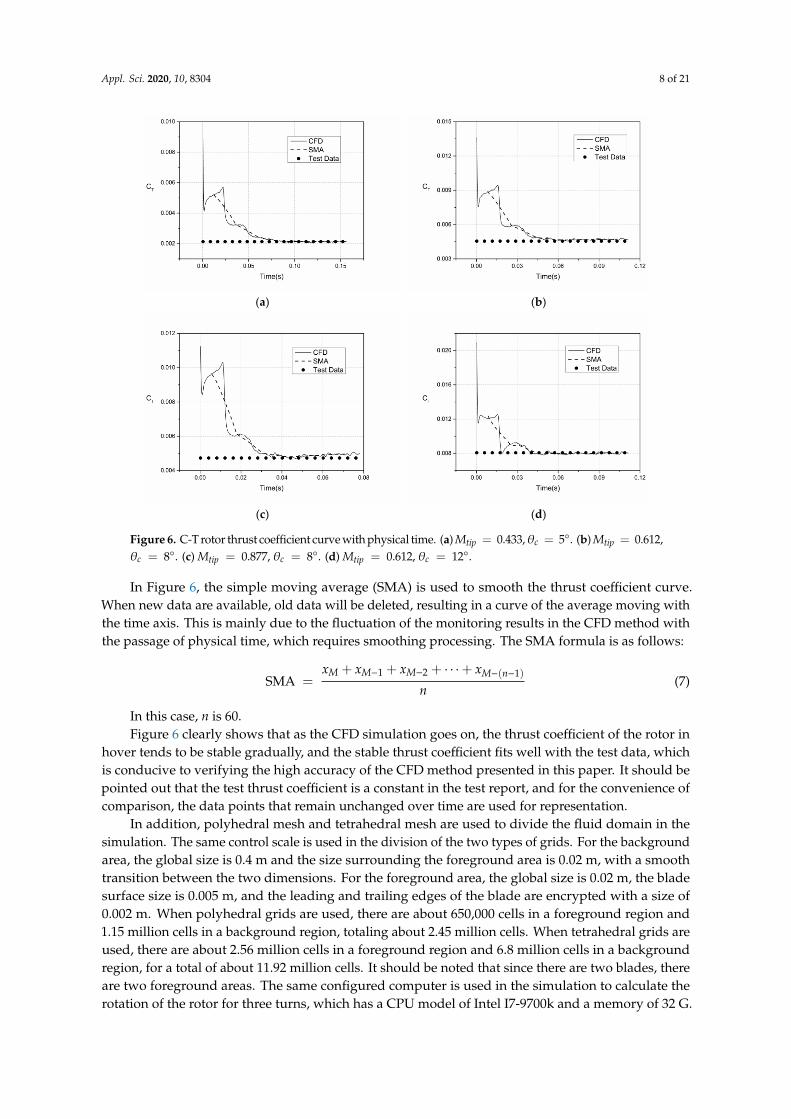
Figure 5. Surface pressure coefficients of C-T rotor at 0.96R profile in hover. (a) Mtip = 0.433, θc = 5.(b) Mtip = 0.612,θc = 8. (c) Mtip = 0.877, θc = 8. (d) Mtip = 0.612,θc = 12.
Figure 5 shows that the pressure coefficient distribution at 0.96R on the blade surface obtained byCFD simulation fits well with the test data. To further verify the accuracy of the simulation, the thrustcoefficient obtained by the simulation was compared with the test data, as shown in Figure 6:
Appl. Sci. 2020, 10, 8304 8 of 21
Appl. Sci. 2020, 10, x FOR PEER REVIEW 8 of 22
Appl. Sci. 2020, 10, x; doi: FOR PEER REVIEW www.mdpi.com/journal/applsci
(c) (d)
Figure 5. Surface pressure coefficients of C-T rotor at 0.96R profile in hover. (a) 𝑀𝑡𝑖𝑝 =
0.433, 𝜃𝑐 = 5° . (b) 𝑀𝑡𝑖𝑝 = 0.612, 𝜃𝑐 = 8°. (c) 𝑀𝑡𝑖𝑝 = 0.877, 𝜃𝑐 = 8°. (d) 𝑀𝑡𝑖𝑝 = 0.612, 𝜃𝑐 =
12°.
Figure 5 shows that the pressure coefficient distribution at 0.96R on the blade surface
obtained by CFD simulation fits well with the test data. To further verify the accuracy of the
simulation, the thrust coefficient obtained by the simulation was compared with the test data,
as shown in Figure 6:
(a) (b)
(c) (d)
Figure 6. C-T rotor thrust coefficient curve with physical time. (a) 𝑀𝑡𝑖𝑝 = 0.433,𝜃𝑐 = 5°. (b)
𝑀𝑡𝑖𝑝 = 0.612,𝜃𝑐 = 8°. (c) 𝑀𝑡𝑖𝑝 = 0.877,𝜃𝑐 = 8°. (d) 𝑀𝑡𝑖𝑝 = 0.612,𝜃𝑐 = 12°.
In Figure 6, the simple moving average (SMA) is used to smooth the thrust coefficient
curve. When new data are available, old data will be deleted, resulting in a curve of the average
moving with the time axis. This is mainly due to the fluctuation of the monitoring results in the
Figure 6. C-T rotor thrust coefficient curve with physical time. (a) Mtip = 0.433,θc = 5. (b) Mtip = 0.612,θc = 8. (c) Mtip = 0.877, θc = 8. (d) Mtip = 0.612, θc = 12.
In Figure 6, the simple moving average (SMA) is used to smooth the thrust coefficient curve.When new data are available, old data will be deleted, resulting in a curve of the average moving withthe time axis. This is mainly due to the fluctuation of the monitoring results in the CFD method withthe passage of physical time, which requires smoothing processing. The SMA formula is as follows:
SMA =xM + xM−1 + xM−2 + · · ·+ xM−(n−1)
n(7)
In this case, n is 60.Figure 6 clearly shows that as the CFD simulation goes on, the thrust coefficient of the rotor in
hover tends to be stable gradually, and the stable thrust coefficient fits well with the test data, whichis conducive to verifying the high accuracy of the CFD method presented in this paper. It should bepointed out that the test thrust coefficient is a constant in the test report, and for the convenience ofcomparison, the data points that remain unchanged over time are used for representation.
In addition, polyhedral mesh and tetrahedral mesh are used to divide the fluid domain in thesimulation. The same control scale is used in the division of the two types of grids. For the backgroundarea, the global size is 0.4 m and the size surrounding the foreground area is 0.02 m, with a smoothtransition between the two dimensions. For the foreground area, the global size is 0.02 m, the bladesurface size is 0.005 m, and the leading and trailing edges of the blade are encrypted with a size of0.002 m. When polyhedral grids are used, there are about 650,000 cells in a foreground region and1.15 million cells in a background region, totaling about 2.45 million cells. When tetrahedral grids areused, there are about 2.56 million cells in a foreground region and 6.8 million cells in a backgroundregion, for a total of about 11.92 million cells. It should be noted that since there are two blades, thereare two foreground areas. The same configured computer is used in the simulation to calculate therotation of the rotor for three turns, which has a CPU model of Intel I7-9700k and a memory of 32 G.
Appl. Sci. 2020, 10, 8304 9 of 21
When tetrahedral mesh is used, the simulation takes about 30 h. However, when hexahedron meshis used, the simulation takes about 18 h, which is only 60% of the time consumption of tetrahedralmesh, and their calculation results are almost the same. Therefore, it is proven that polyhedral meshcan greatly improve the efficiency of calculation while ensuring high accuracy. The same conclusioncan be obtained in the following several validation examples, which proves that compared with thetraditional tetrahedral mesh, the polyhedral mesh has higher computational efficiency in aerodynamicsimulation of helicopters.
3.2. AH-1G Rotor in Forward Flight
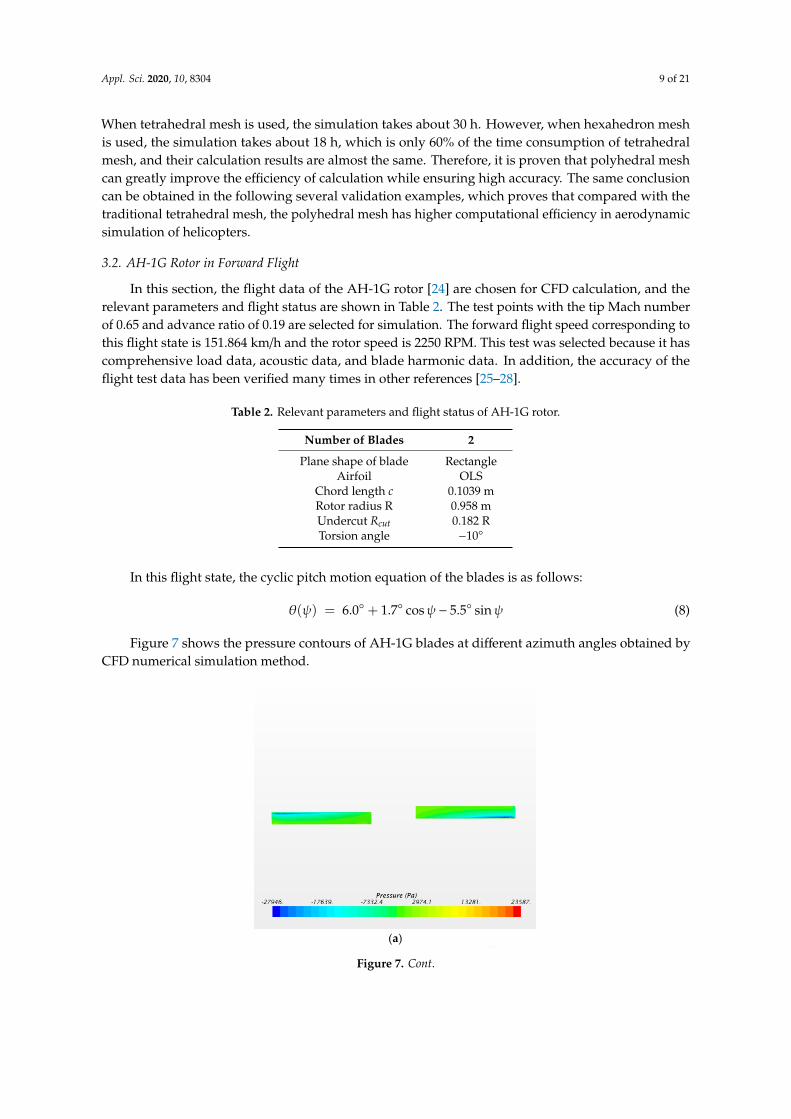
In this section, the flight data of the AH-1G rotor [24] are chosen for CFD calculation, and therelevant parameters and flight status are shown in Table 2. The test points with the tip Mach numberof 0.65 and advance ratio of 0.19 are selected for simulation. The forward flight speed corresponding tothis flight state is 151.864 km/h and the rotor speed is 2250 RPM. This test was selected because it hascomprehensive load data, acoustic data, and blade harmonic data. In addition, the accuracy of theflight test data has been verified many times in other references [25–28].
Table 2. Relevant parameters and flight status of AH-1G rotor.
Number of Blades 2
Plane shape of blade RectangleAirfoil OLS
Chord length c 0.1039 mRotor radius R 0.958 mUndercut Rcut 0.182 RTorsion angle −10
In this flight state, the cyclic pitch motion equation of the blades is as follows:
θ(ψ) = 6.0 + 1.7 cosψ− 5.5 sinψ (8)
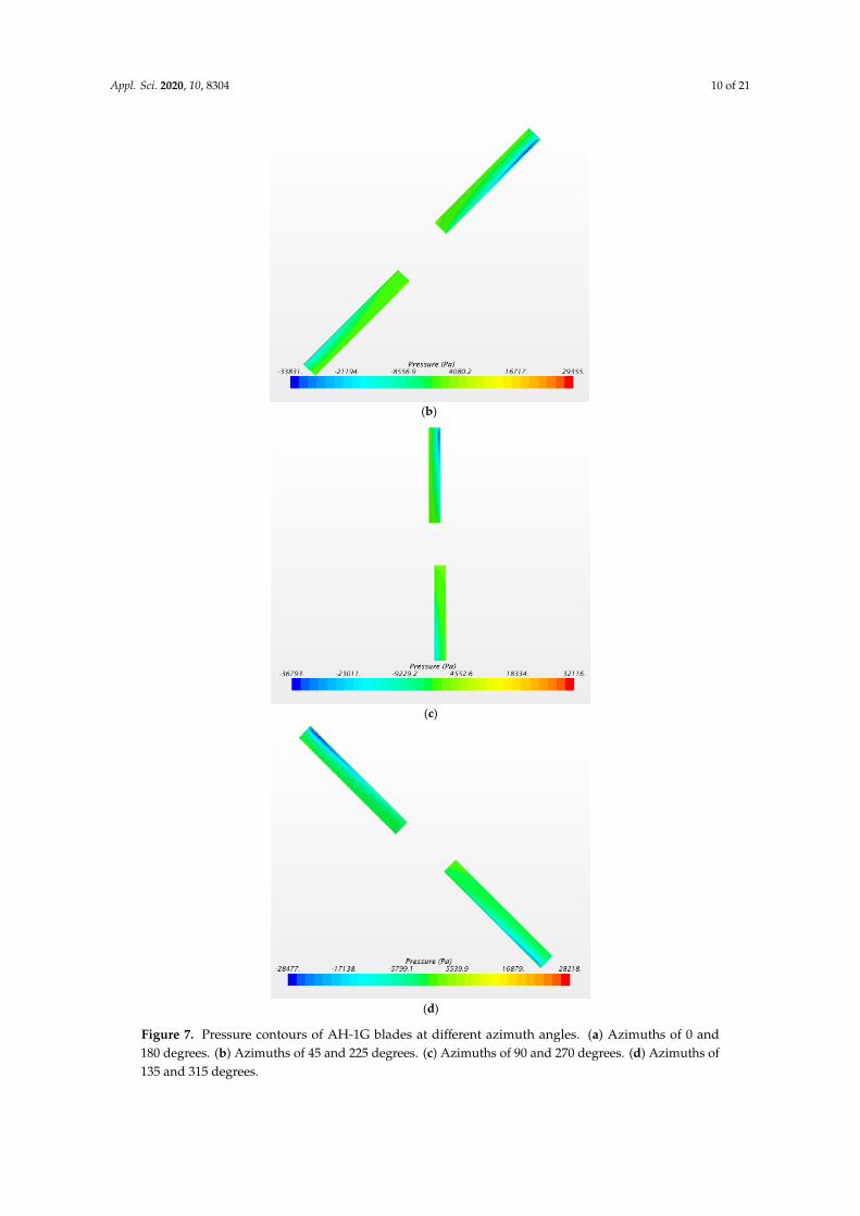
Figure 7 shows the pressure contours of AH-1G blades at different azimuth angles obtained byCFD numerical simulation method.
Appl. Sci. 2020, 10, x FOR PEER REVIEW 10 of 22
Appl. Sci. 2020, 10, x; doi: FOR PEER REVIEW www.mdpi.com/journal/applsci
In this flight state, the cyclic pitch motion equation of the blades is as follows:
𝜃(𝜓) = 6.0° + 1.7° cos𝜓 − 5.5° sin𝜓 (8)
Figure 7 shows the pressure contours of AH-1G blades at different azimuth angles
obtained by CFD numerical simulation method.
(a)
(b)
Figure 7. Cont.
Appl. Sci. 2020, 10, 8304 10 of 21
Appl. Sci. 2020, 10, x FOR PEER REVIEW 10 of 22
Appl. Sci. 2020, 10, x; doi: FOR PEER REVIEW www.mdpi.com/journal/applsci
In this flight state, the cyclic pitch motion equation of the blades is as follows:
𝜃(𝜓) = 6.0° + 1.7° cos𝜓 − 5.5° sin𝜓 (8)
Figure 7 shows the pressure contours of AH-1G blades at different azimuth angles
obtained by CFD numerical simulation method.
(a)
(b)
Appl. Sci. 2020, 10, x FOR PEER REVIEW 11 of 22
Appl. Sci. 2020, 10, x; doi: FOR PEER REVIEW www.mdpi.com/journal/applsci
(c)
(d)
Figure 7. Pressure contours of AH-1G blades at different azimuth angles. (a) Azimuths of 0
and 180 degrees. (b) Azimuths of 45 and 225 degrees. (c) Azimuths of 90 and 270 degrees. (d)
Azimuths of 135 and 315 degrees.
According to Figure 7, it is not difficult to see that the shock waves at the blade tip in the
azimuth range of 0° to 180° are more obvious than those at the azimuth range of 180° to 360°.
The shock waves at the blade tip are the strongest at the azimuth angle of 90°, which is
consistent with the aerodynamic theory of the helicopter.
Considering that only the overall trend of the simulation results can be seen in Figure 7,
in order to more accurately judge the accuracy of the simulation, the pressure coefficient
distribution of different azimuth angles and different blade profiles calculated by CFD
numerical simulation method was compared with the experimental values, as shown in Figure
8.
Figure 7. Pressure contours of AH-1G blades at different azimuth angles. (a) Azimuths of 0 and180 degrees. (b) Azimuths of 45 and 225 degrees. (c) Azimuths of 90 and 270 degrees. (d) Azimuths of135 and 315 degrees.
Appl. Sci. 2020, 10, 8304 11 of 21
According to Figure 7, it is not difficult to see that the shock waves at the blade tip in the azimuthrange of 0 to 180 are more obvious than those at the azimuth range of 180 to 360. The shock wavesat the blade tip are the strongest at the azimuth angle of 90, which is consistent with the aerodynamictheory of the helicopter.
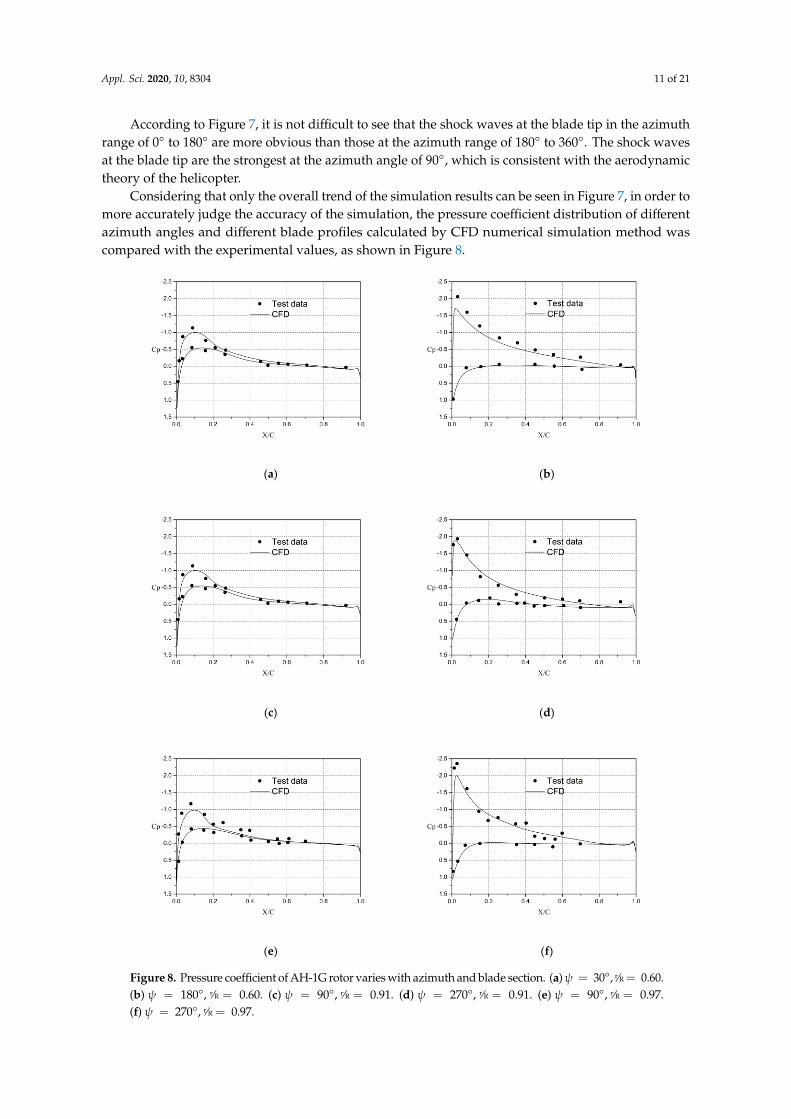
Considering that only the overall trend of the simulation results can be seen in Figure 7, in order tomore accurately judge the accuracy of the simulation, the pressure coefficient distribution of differentazimuth angles and different blade profiles calculated by CFD numerical simulation method wascompared with the experimental values, as shown in Figure 8.
Appl. Sci. 2020, 10, x FOR PEER REVIEW 12 of 22
Appl. Sci. 2020, 10, x; doi: FOR PEER REVIEW www.mdpi.com/journal/applsci
(a) (b)
(c) (d)
(e) (f)
Figure 8. Pressure coefficient of AH-1G rotor varies with azimuth and blade section. (a) ψ =
30°, 𝑟 𝑅⁄ = 0.60. (b) ψ = 180°, 𝑟 𝑅⁄ = 0.60. (c) ψ = 90°, 𝑟 𝑅⁄ = 0.91. (d) ψ = 270°, 𝑟 𝑅⁄ = 0.91. (e)
ψ = 90°, 𝑟 𝑅⁄ = 0.97. (f) ψ = 270°, 𝑟 𝑅⁄ = 0.97.
In Figure 9, the curves of normal force coefficient with azimuth angle at four different
section positions on the blade calculated by CFD simulation are given and compared with the
test data. According to the data in the figure, when the azimuth angle of the advancing blade
is about 70° to 90° or the retreating blade is near an azimuth of about 270°, there will be strong
blade/vortex interference, resulting in abrupt change of aerodynamic force in the blade section,
which makes it more difficult to simulate the rotor flow field in forward flight state.
Figure 8. Pressure coefficient of AH-1G rotor varies with azimuth and blade section. (a)ψ = 30, r⁄R = 0.60.(b) ψ = 180, r⁄R = 0.60. (c) ψ = 90, r⁄R = 0.91. (d) ψ = 270, r⁄R = 0.91. (e) ψ = 90, r⁄R = 0.97.(f) ψ = 270, r⁄R = 0.97.
Appl. Sci. 2020, 10, 8304 12 of 21
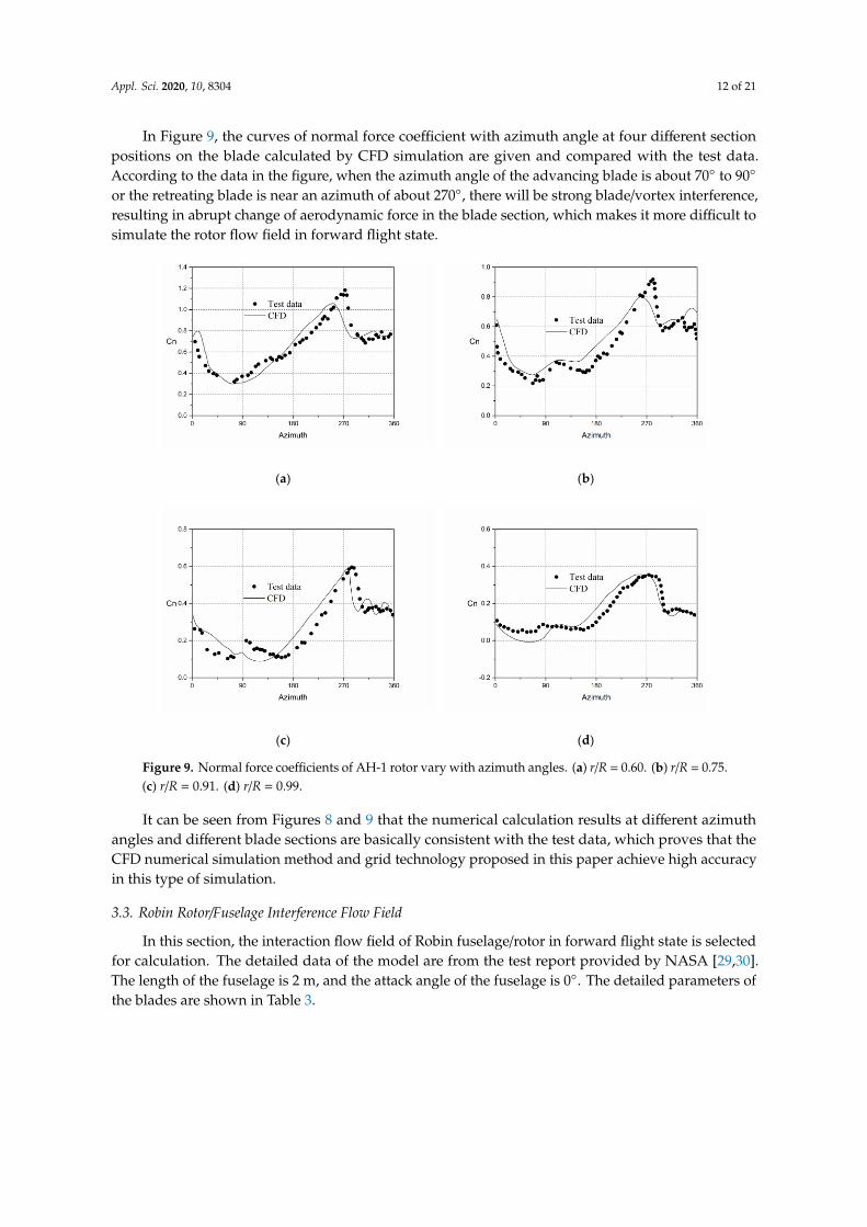
In Figure 9, the curves of normal force coefficient with azimuth angle at four different sectionpositions on the blade calculated by CFD simulation are given and compared with the test data.According to the data in the figure, when the azimuth angle of the advancing blade is about 70 to 90
or the retreating blade is near an azimuth of about 270, there will be strong blade/vortex interference,resulting in abrupt change of aerodynamic force in the blade section, which makes it more difficult tosimulate the rotor flow field in forward flight state.
Appl. Sci. 2020, 10, x FOR PEER REVIEW 13 of 22
Appl. Sci. 2020, 10, x; doi: FOR PEER REVIEW www.mdpi.com/journal/applsci
(a) (b)
(c) (d)
Figure 9. Normal force coefficients of AH-1 rotor vary with azimuth angles. (a) r/R = 0.60. (b)
r/R = 0.75. (c) r/R = 0.91. (d) r/R = 0.99.
It can be seen from Figures 8 and 9 that the numerical calculation results at different
azimuth angles and different blade sections are basically consistent with the test data, which
proves that the CFD numerical simulation method and grid technology proposed in this paper
achieve high accuracy in this type of simulation.
3.3. Robin Rotor/Fuselage Interference Flow Field
In this section, the interaction flow field of Robin fuselage/rotor in forward flight state is
selected for calculation. The detailed data of the model are from the test report provided by
NASA [29,30]. The length of the fuselage is 2 m, and the attack angle of the fuselage is 0 °. The
detailed parameters of the blades are shown in Table 3.
Table 3. Detailed parameters of the blades in the Robin fuselage/rotor interference flow field.
Number of Blades 4
Airfoil NACA0012
Chord length c 0.0663m
Rotor radius R 0.8604m
Undercut 𝑅𝑐𝑢𝑡 0.24R
Rotation speed 𝑛 2000RPM
Torsion angle −8°
Figure 9. Normal force coefficients of AH-1 rotor vary with azimuth angles. (a) r/R = 0.60. (b) r/R = 0.75.(c) r/R = 0.91. (d) r/R = 0.99.
It can be seen from Figures 8 and 9 that the numerical calculation results at different azimuthangles and different blade sections are basically consistent with the test data, which proves that theCFD numerical simulation method and grid technology proposed in this paper achieve high accuracyin this type of simulation.
3.3. Robin Rotor/Fuselage Interference Flow Field
In this section, the interaction flow field of Robin fuselage/rotor in forward flight state is selectedfor calculation. The detailed data of the model are from the test report provided by NASA [29,30].The length of the fuselage is 2 m, and the attack angle of the fuselage is 0. The detailed parameters ofthe blades are shown in Table 3.
Appl. Sci. 2020, 10, 8304 13 of 21
Table 3. Detailed parameters of the blades in the Robin fuselage/rotor interference flow field.
Number of Blades 4
Airfoil NACA0012Chord length c 0.0663 mRotor radius R 0.8604 mUndercut Rcut 0.24 R
Rotation speed n 2000 RPMTorsion angle −8
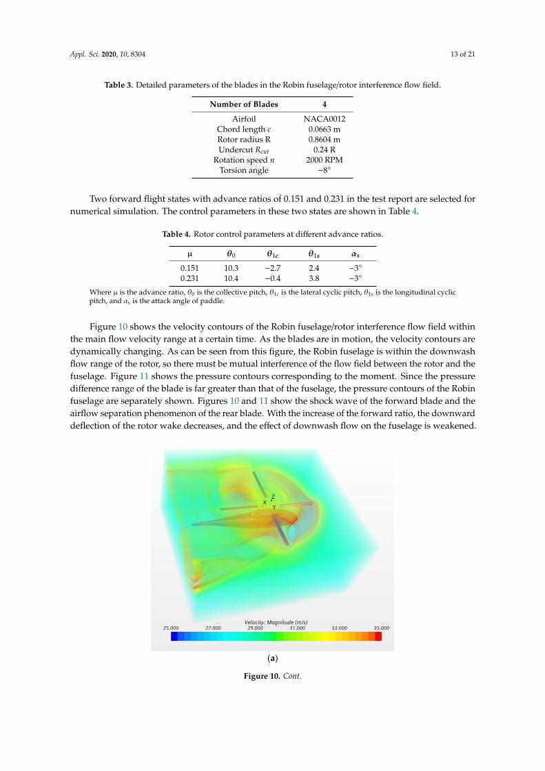
Two forward flight states with advance ratios of 0.151 and 0.231 in the test report are selected fornumerical simulation. The control parameters in these two states are shown in Table 4.
Table 4. Rotor control parameters at different advance ratios.
µ θ0 θ1c θ1s αs
0.151 10.3 −2.7 2.4 −3
0.231 10.4 −0.4 3.8 −3
Where µ is the advance ratio, θ0 is the collective pitch, θ1c is the lateral cyclic pitch, θ1s is the longitudinal cyclicpitch, and αs is the attack angle of paddle.
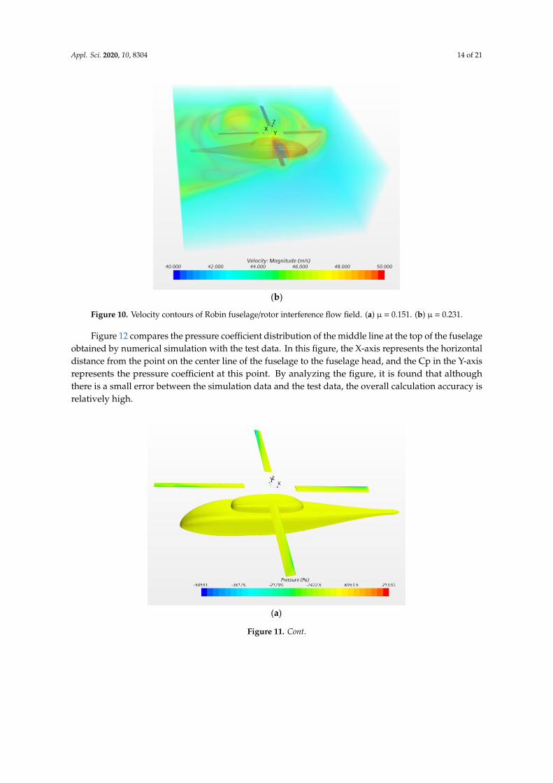
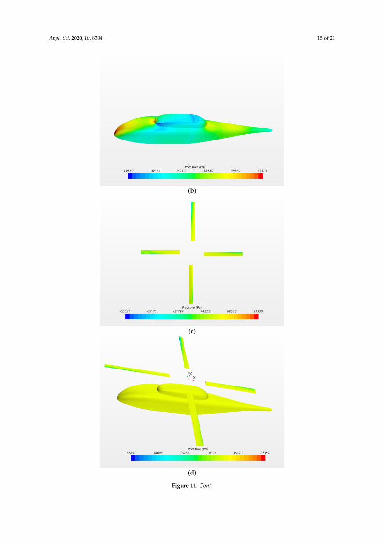
Figure 10 shows the velocity contours of the Robin fuselage/rotor interference flow field withinthe main flow velocity range at a certain time. As the blades are in motion, the velocity contours aredynamically changing. As can be seen from this figure, the Robin fuselage is within the downwashflow range of the rotor, so there must be mutual interference of the flow field between the rotor and thefuselage. Figure 11 shows the pressure contours corresponding to the moment. Since the pressuredifference range of the blade is far greater than that of the fuselage, the pressure contours of the Robinfuselage are separately shown. Figures 10 and 11 show the shock wave of the forward blade and theairflow separation phenomenon of the rear blade. With the increase of the forward ratio, the downwarddeflection of the rotor wake decreases, and the effect of downwash flow on the fuselage is weakened.
Appl. Sci. 2020, 10, x FOR PEER REVIEW 14 of 22
Appl. Sci. 2020, 10, x; doi: FOR PEER REVIEW www.mdpi.com/journal/applsci
Two forward flight states with advance ratios of 0.151 and 0.231 in the test report are
selected for numerical simulation. The control parameters in these two states are shown in
Table 4.
Table 4. Rotor control parameters at different advance ratios.
μ 𝜽𝟎 𝜽𝟏𝒄 𝜽𝟏𝒔 𝜶𝒔
0.151 10.3 −2.7 2.4 −3°
0.231 10.4 −0.4 3.8 −3°
Where μ is the advance ratio, 𝜃0 is the collective pitch, 𝜃1𝑐 is the lateral cyclic pitch, 𝜃1𝑠 is the
longitudinal cyclic pitch, and 𝛼𝑠 is the attack angle of paddle.
Figure 10 shows the velocity contours of the Robin fuselage/rotor interference flow field
within the main flow velocity range at a certain time. As the blades are in motion, the velocity
contours are dynamically changing. As can be seen from this figure, the Robin fuselage is
within the downwash flow range of the rotor, so there must be mutual interference of the flow
field between the rotor and the fuselage. Figure 11 shows the pressure contours corresponding
to the moment. Since the pressure difference range of the blade is far greater than that of the
fuselage, the pressure contours of the Robin fuselage are separately shown. Figures 10 and 11
show the shock wave of the forward blade and the airflow separation phenomenon of the rear
blade. With the increase of the forward ratio, the downward deflection of the rotor wake
decreases, and the effect of downwash flow on the fuselage is weakened.
(a)
Figure 10. Cont.
Appl. Sci. 2020, 10, 8304 14 of 21Appl. Sci. 2020, 10, x FOR PEER REVIEW 15 of 22
Appl. Sci. 2020, 10, x; doi: FOR PEER REVIEW www.mdpi.com/journal/applsci
(b)
Figure 10. Velocity contours of Robin fuselage/rotor interference flow field. (a) μ = 0.151. (b) μ
= 0.231.
(a)
Figure 10. Velocity contours of Robin fuselage/rotor interference flow field. (a) µ = 0.151. (b) µ = 0.231.
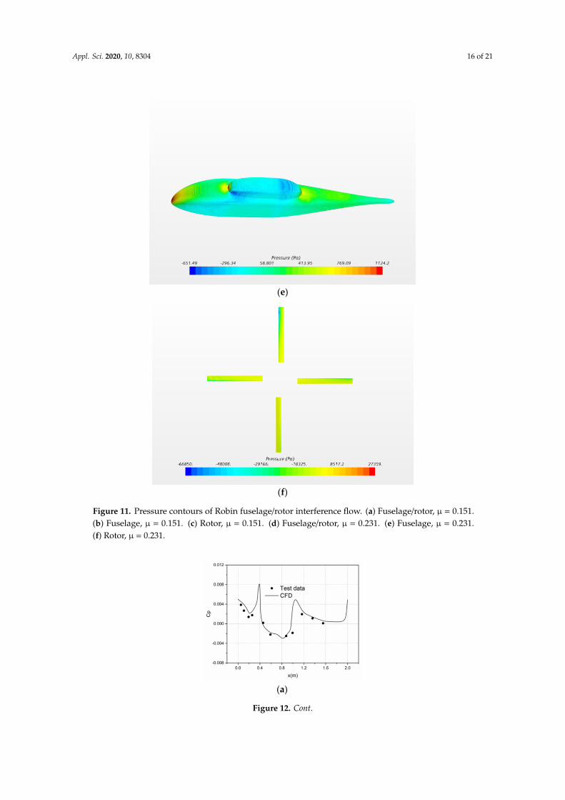
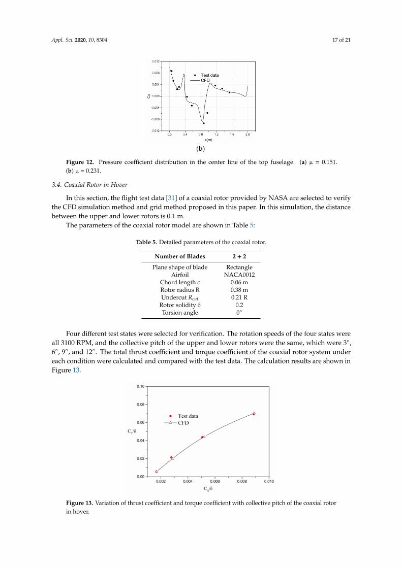
Figure 12 compares the pressure coefficient distribution of the middle line at the top of the fuselageobtained by numerical simulation with the test data. In this figure, the X-axis represents the horizontaldistance from the point on the center line of the fuselage to the fuselage head, and the Cp in the Y-axisrepresents the pressure coefficient at this point. By analyzing the figure, it is found that althoughthere is a small error between the simulation data and the test data, the overall calculation accuracy isrelatively high.
Appl. Sci. 2020, 10, x FOR PEER REVIEW 15 of 22
Appl. Sci. 2020, 10, x; doi: FOR PEER REVIEW www.mdpi.com/journal/applsci
(b)
Figure 10. Velocity contours of Robin fuselage/rotor interference flow field. (a) μ = 0.151. (b) μ
= 0.231.
(a)
Figure 11. Cont.
Appl. Sci. 2020, 10, 8304 15 of 21Appl. Sci. 2020, 10, x FOR PEER REVIEW 16 of 22
Appl. Sci. 2020, 10, x; doi: FOR PEER REVIEW www.mdpi.com/journal/applsci
(b)
(c)
(d)
Figure 11. Cont.
Appl. Sci. 2020, 10, 8304 16 of 21
Appl. Sci. 2020, 10, x FOR PEER REVIEW 17 of 22
Appl. Sci. 2020, 10, x; doi: FOR PEER REVIEW www.mdpi.com/journal/applsci
(e)
(f)
Figure 11. Pressure contours of Robin fuselage/rotor interference flow. (a) Fuselage/rotor, μ =
0.151. (b) Fuselage, μ = 0.151. (c) Rotor, μ = 0.151. (d) Fuselage/rotor, μ = 0.231. (e) Fuselage, μ
= 0.231. (f) Rotor, μ = 0.231.
Figure 12 compares the pressure coefficient distribution of the middle line at the top of the
fuselage obtained by numerical simulation with the test data. In this figure, the X-axis
represents the horizontal distance from the point on the center line of the fuselage to the
fuselage head, and the Cp in the Y-axis represents the pressure coefficient at this point. By
analyzing the figure, it is found that although there is a small error between the simulation data
and the test data, the overall calculation accuracy is relatively high.
Figure 11. Pressure contours of Robin fuselage/rotor interference flow. (a) Fuselage/rotor, µ = 0.151.(b) Fuselage, µ = 0.151. (c) Rotor, µ = 0.151. (d) Fuselage/rotor, µ = 0.231. (e) Fuselage, µ = 0.231.(f) Rotor, µ = 0.231.Appl. Sci. 2020, 10, x FOR PEER REVIEW 18 of 22
Appl. Sci. 2020, 10, x; doi: FOR PEER REVIEW www.mdpi.com/journal/applsci
(a)
(b)
Figure 12. Pressure coefficient distribution in the center line of the top fuselage. (a) μ = 0.151.
(b) μ = 0.231.
3.4. Coaxial Rotor in Hover
In this section, the flight test data [31] of a coaxial rotor provided by NASA are selected to
verify the CFD simulation method and grid method proposed in this paper. In this simulation,
the distance between the upper and lower rotors is 0.1 m.
The parameters of the coaxial rotor model are shown in Table 5:
Table 5. Detailed parameters of the coaxial rotor.
Number of Blades 2 + 2
Plane shape of blade Rectangle
Airfoil NACA0012
Chord length c 0.06m
Rotor radius R 0.38m
Undercut 𝑅𝑐𝑢𝑡 0.21R
Rotor solidity 𝛿 0.2
Torsion angle 0°
Four different test states were selected for verification. The rotation speeds of the four
states were all 3100 RPM, and the collective pitch of the upper and lower rotors were the same,
which were 3°, 6°, 9°, and 12°. The total thrust coefficient and torque coefficient of the coaxial
rotor system under each condition were calculated and compared with the test data. The
calculation results are shown in Figure 13.
Figure 12. Cont.
Appl. Sci. 2020, 10, 8304 17 of 21
Appl. Sci. 2020, 10, x FOR PEER REVIEW 18 of 22
Appl. Sci. 2020, 10, x; doi: FOR PEER REVIEW www.mdpi.com/journal/applsci
(a)
(b)
Figure 12. Pressure coefficient distribution in the center line of the top fuselage. (a) μ = 0.151.
(b) μ = 0.231.
3.4. Coaxial Rotor in Hover
In this section, the flight test data [31] of a coaxial rotor provided by NASA are selected to
verify the CFD simulation method and grid method proposed in this paper. In this simulation,
the distance between the upper and lower rotors is 0.1 m.
The parameters of the coaxial rotor model are shown in Table 5:
Table 5. Detailed parameters of the coaxial rotor.
Number of Blades 2 + 2
Plane shape of blade Rectangle
Airfoil NACA0012
Chord length c 0.06m
Rotor radius R 0.38m
Undercut 𝑅𝑐𝑢𝑡 0.21R
Rotor solidity 𝛿 0.2
Torsion angle 0°
Four different test states were selected for verification. The rotation speeds of the four
states were all 3100 RPM, and the collective pitch of the upper and lower rotors were the same,
which were 3°, 6°, 9°, and 12°. The total thrust coefficient and torque coefficient of the coaxial
rotor system under each condition were calculated and compared with the test data. The
calculation results are shown in Figure 13.
Figure 12. Pressure coefficient distribution in the center line of the top fuselage. (a) µ = 0.151.(b) µ = 0.231.
3.4. Coaxial Rotor in Hover
In this section, the flight test data [31] of a coaxial rotor provided by NASA are selected to verifythe CFD simulation method and grid method proposed in this paper. In this simulation, the distancebetween the upper and lower rotors is 0.1 m.
The parameters of the coaxial rotor model are shown in Table 5:
Table 5. Detailed parameters of the coaxial rotor.
Number of Blades 2 + 2
Plane shape of blade RectangleAirfoil NACA0012
Chord length c 0.06 mRotor radius R 0.38 mUndercut Rcut 0.21 R
Rotor solidity δ 0.2Torsion angle 0
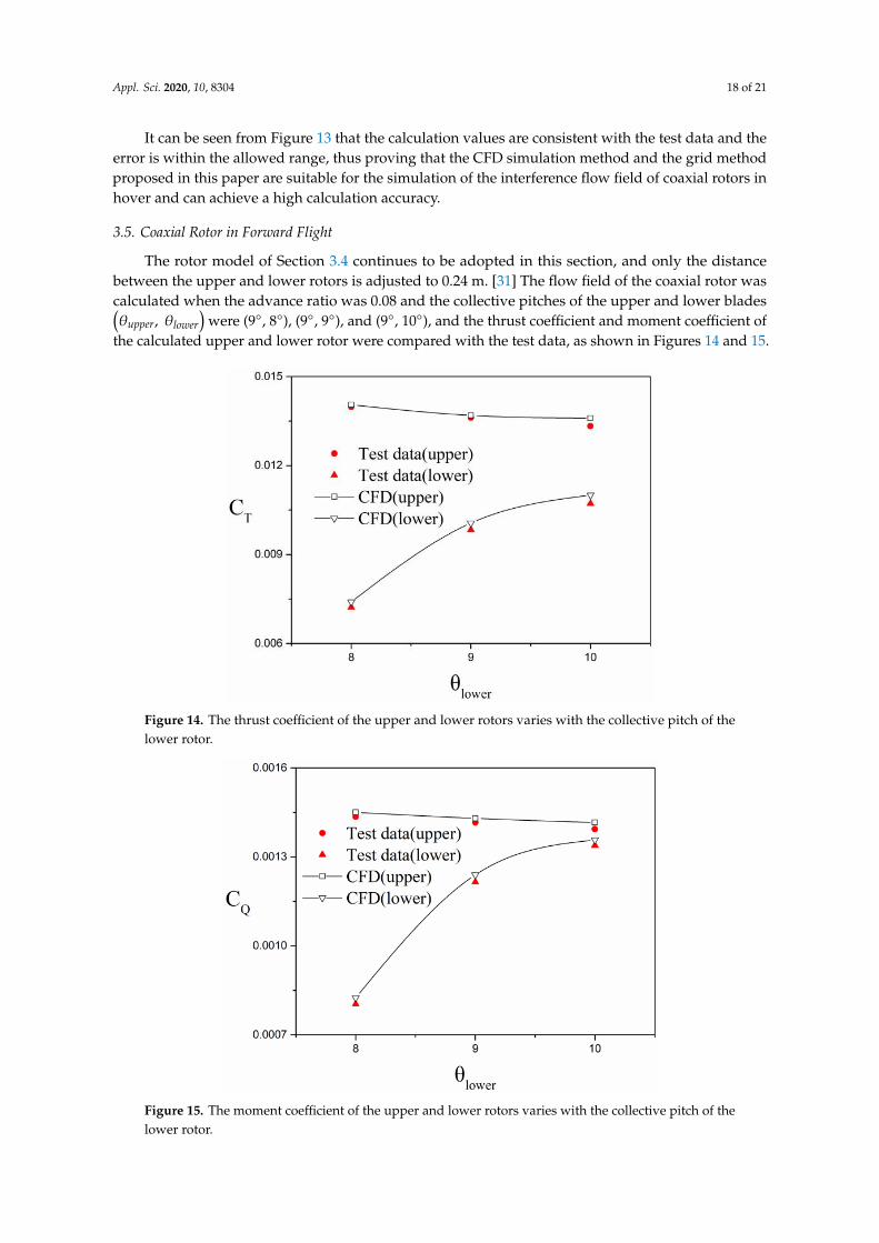
Four different test states were selected for verification. The rotation speeds of the four states wereall 3100 RPM, and the collective pitch of the upper and lower rotors were the same, which were 3,6, 9, and 12. The total thrust coefficient and torque coefficient of the coaxial rotor system undereach condition were calculated and compared with the test data. The calculation results are shown inFigure 13.
Appl. Sci. 2020, 10, x FOR PEER REVIEW 19 of 22
Appl. Sci. 2020, 10, x; doi: FOR PEER REVIEW www.mdpi.com/journal/applsci
Figure 13. Variation of thrust coefficient and torque coefficient with collective pitch of the
coaxial rotor in hover.
It can be seen from Figure 13 that the calculation values are consistent with the test data
and the error is within the allowed range, thus proving that the CFD simulation method and
the grid method proposed in this paper are suitable for the simulation of the interference flow
field of coaxial rotors in hover and can achieve a high calculation accuracy.
3.5. Coaxial Rotor in Forward Flight
The rotor model of Section 3.4 continues to be adopted in this section, and only the
distance between the upper and lower rotors is adjusted to 0.24 m. [31] The flow field of the
coaxial rotor was calculated when the advance ratio was 0.08 and the collective pitches of the
upper and lower blades (𝜃𝑢𝑝𝑝𝑒𝑟 , 𝜃𝑙𝑜𝑤𝑒𝑟) were (9°, 8°), (9°, 9°), and (9°, 10°), and the thrust
coefficient and moment coefficient of the calculated upper and lower rotor were compared with
the test data, as shown in Figures 14 and 15.
Figure 14. The thrust coefficient of the upper and lower rotors varies with the collective pitch
of the lower rotor.
Figure 13. Variation of thrust coefficient and torque coefficient with collective pitch of the coaxial rotorin hover.
Appl. Sci. 2020, 10, 8304 18 of 21
It can be seen from Figure 13 that the calculation values are consistent with the test data and theerror is within the allowed range, thus proving that the CFD simulation method and the grid methodproposed in this paper are suitable for the simulation of the interference flow field of coaxial rotors inhover and can achieve a high calculation accuracy.
3.5. Coaxial Rotor in Forward Flight
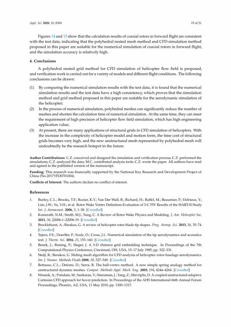
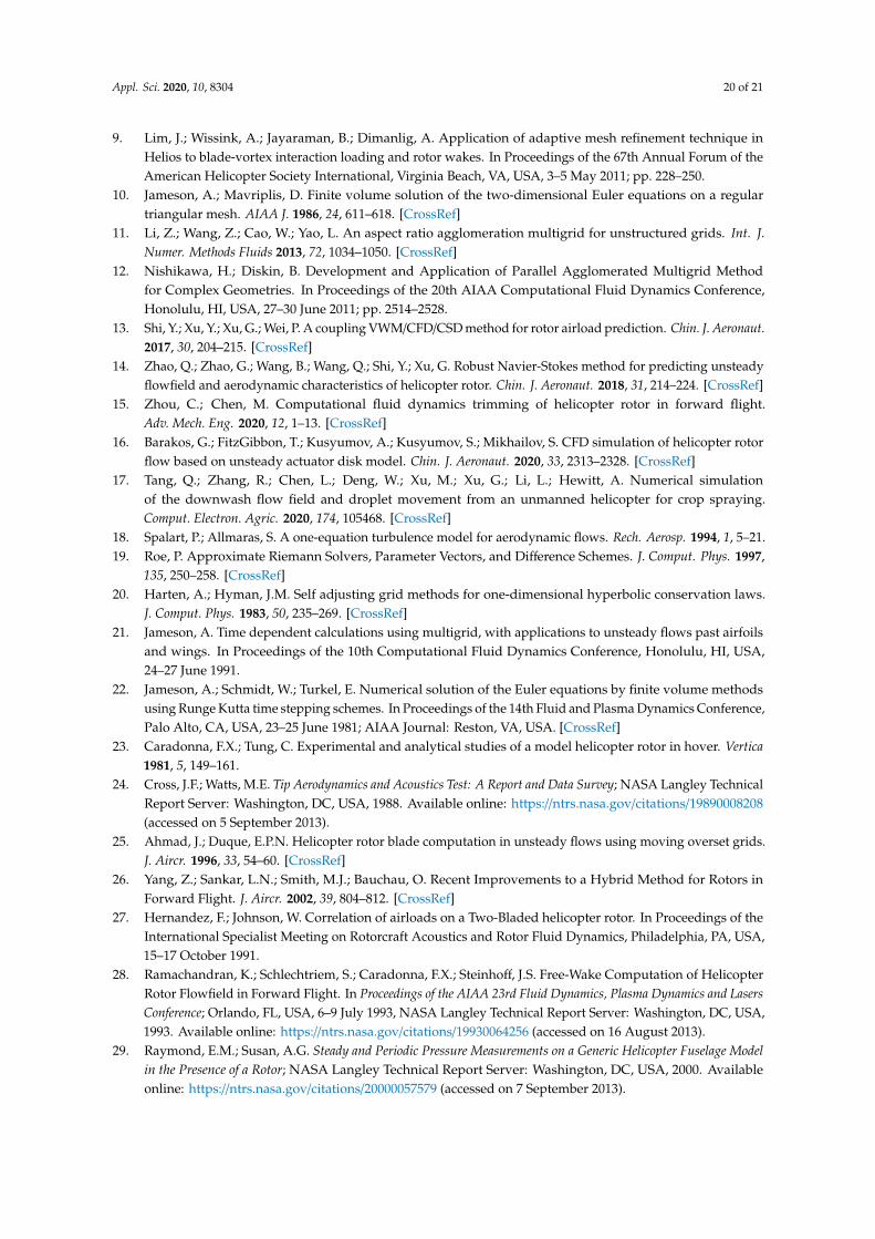
The rotor model of Section 3.4 continues to be adopted in this section, and only the distancebetween the upper and lower rotors is adjusted to 0.24 m. [31] The flow field of the coaxial rotor wascalculated when the advance ratio was 0.08 and the collective pitches of the upper and lower blades(θupper, θlower
)were (9, 8), (9, 9), and (9, 10), and the thrust coefficient and moment coefficient of
the calculated upper and lower rotor were compared with the test data, as shown in Figures 14 and 15.
Appl. Sci. 2020, 10, x FOR PEER REVIEW 19 of 22
Appl. Sci. 2020, 10, x; doi: FOR PEER REVIEW www.mdpi.com/journal/applsci
Figure 13. Variation of thrust coefficient and torque coefficient with collective pitch of the
coaxial rotor in hover.
It can be seen from Figure 13 that the calculation values are consistent with the test data
and the error is within the allowed range, thus proving that the CFD simulation method and
the grid method proposed in this paper are suitable for the simulation of the interference flow
field of coaxial rotors in hover and can achieve a high calculation accuracy.
3.5. Coaxial Rotor in Forward Flight
The rotor model of Section 3.4 continues to be adopted in this section, and only the
distance between the upper and lower rotors is adjusted to 0.24 m. [31] The flow field of the
coaxial rotor was calculated when the advance ratio was 0.08 and the collective pitches of the
upper and lower blades (𝜃𝑢𝑝𝑝𝑒𝑟 , 𝜃𝑙𝑜𝑤𝑒𝑟) were (9°, 8°), (9°, 9°), and (9°, 10°), and the thrust
coefficient and moment coefficient of the calculated upper and lower rotor were compared with
the test data, as shown in Figures 14 and 15.
Figure 14. The thrust coefficient of the upper and lower rotors varies with the collective pitch
of the lower rotor.
Figure 14. The thrust coefficient of the upper and lower rotors varies with the collective pitch of thelower rotor.
Appl. Sci. 2020, 10, x FOR PEER REVIEW 20 of 22
Appl. Sci. 2020, 10, x; doi: FOR PEER REVIEW www.mdpi.com/journal/applsci
Figure 15. The moment coefficient of the upper and lower rotors varies with the collective pitch
of the lower rotor.
Figures 14 and 15 show that the calculation results of coaxial rotors in forward flight are
consistent with the test data, indicating that the polyhedral nested mesh method and CFD
simulation method proposed in this paper are suitable for the numerical simulation of coaxial
rotors in forward flight, and the simulation accuracy is relatively high.
4. Conclusions
A polyhedral nested grid method for CFD simulation of helicopter flow field is proposed,
and verification work is carried out for a variety of models and different flight conditions. The
following conclusions can be drawn:
(1) By comparing the numerical simulation results with the test data, it is found that the
numerical simulation results and the test data have a high consistency, which proves that
the simulation method and grid method proposed in this paper are suitable for the
aerodynamic simulation of the helicopter;
(2) In the process of numerical simulation, polyhedral meshes can significantly reduce the
number of meshes and shorten the calculation time of numerical simulation. At the same
time, they can meet the requirement of high precision of helicopter flow field simulation,
which has high engineering application value;
(3) At present, there are many applications of structural grids in CFD simulation of
helicopters. With the increase in the complexity of helicopter model and motion form, the
time cost of structural grids becomes very high, and the new unstructured mesh
represented by polyhedral mesh will undoubtedly be the research hotspot in the future.
Author Contributions: C.Z. conceived and designed the simulation and verification process;
C.Z. performed the simulations; C.Z. analyzed the data; M.C. contributed analysis tools; C.Z.
wrote the paper. All authors have read and agreed to the published version of the manuscript.
Funding: This research was financially supported by the National Key Research and
Development Project of China (No.2017YFD0701004).
Conflicts of Interest: The authors declare no conflict of interest.
Figure 15. The moment coefficient of the upper and lower rotors varies with the collective pitch of thelower rotor.
Appl. Sci. 2020, 10, 8304 19 of 21
Figures 14 and 15 show that the calculation results of coaxial rotors in forward flight are consistentwith the test data, indicating that the polyhedral nested mesh method and CFD simulation methodproposed in this paper are suitable for the numerical simulation of coaxial rotors in forward flight,and the simulation accuracy is relatively high.
4. Conclusions
A polyhedral nested grid method for CFD simulation of helicopter flow field is proposed,and verification work is carried out for a variety of models and different flight conditions. The followingconclusions can be drawn:
(1) By comparing the numerical simulation results with the test data, it is found that the numericalsimulation results and the test data have a high consistency, which proves that the simulationmethod and grid method proposed in this paper are suitable for the aerodynamic simulation ofthe helicopter;
(2) In the process of numerical simulation, polyhedral meshes can significantly reduce the number ofmeshes and shorten the calculation time of numerical simulation. At the same time, they can meetthe requirement of high precision of helicopter flow field simulation, which has high engineeringapplication value;
(3) At present, there are many applications of structural grids in CFD simulation of helicopters. Withthe increase in the complexity of helicopter model and motion form, the time cost of structuralgrids becomes very high, and the new unstructured mesh represented by polyhedral mesh willundoubtedly be the research hotspot in the future.
Author Contributions: C.Z. conceived and designed the simulation and verification process; C.Z. performed thesimulations; C.Z. analyzed the data; M.C. contributed analysis tools; C.Z. wrote the paper. All authors have readand agreed to the published version of the manuscript.
Funding: This research was financially supported by the National Key Research and Development Project ofChina (No.2017YFD0701004).
Conflicts of Interest: The authors declare no conflict of interest.
References
1. Burley, C.L.; Brooks, T.F.; Rozier, K.Y.; Van Der Wall, B.; Richard, H.; Raffel, M.; Beaumier, P.; Delrieux, Y.;Lim, J.W.; Yu, Y.H.; et al. Rotor Wake Vortex Definition-Evaluation of 3-C PIV Results of the HART-II Study.Int. J. Aeroacoust. 2006, 5, 1–38. [CrossRef]
2. Komerath, N.M.; Smith, M.J.; Tung, C. A Review of Rotor Wake Physics and Modeling. J. Am. Helicopter Soc.2011, 56, 22006-1–22006-19. [CrossRef]
3. Brocklehurst, A.; Barakos, G. A review of helicopter rotor blade tip shapes. Prog. Aerosp. Sci. 2013, 56, 35–74.[CrossRef]
4. Tejero, F.E.; Doerffer, P.; Szulc, O.; Cross, J.L. Numerical simulation of the tip aerodynamics and acousticstest. J. Therm. Sci. 2016, 25, 153–160. [CrossRef]
5. Benek, J.; Buning, P.; Steger, J. A 3-D chimera grid embedding technique. In Proceedings of the 7thComputational Physics Conference, Cincinnati, OH, USA, 15–17 July 1985; pp. 322–331.
6. Steijl, R.; Barakos, G. Sliding mesh algorithm for CFD analysis of helicopter rotor-fuselage aerodynamics.Int. J. Numer. Methods Fluids 2008, 58, 527–549. [CrossRef]
7. Bottasso, C.L.; Detomi, D.; Serra, R. The ball-vertex method: A new simple spring analogy method forunstructured dynamic meshes. Comput. Methods Appl. Mech. Eng. 2005, 194, 4244–4264. [CrossRef]
8. Wissink, A.; Potsdam, M.; Sankaran, V.; Sitaraman, J.; Yang, Z.; Mavriplis, D. A coupled unstructured-adaptiveCartesian CFD approach for hover prediction. In Proceedings of the AHS International 66th Annual ForumProceedings, Phoenix, AZ, USA, 11 May 2010; pp. 1300–1317.
Appl. Sci. 2020, 10, 8304 20 of 21
9. Lim, J.; Wissink, A.; Jayaraman, B.; Dimanlig, A. Application of adaptive mesh refinement technique inHelios to blade-vortex interaction loading and rotor wakes. In Proceedings of the 67th Annual Forum of theAmerican Helicopter Society International, Virginia Beach, VA, USA, 3–5 May 2011; pp. 228–250.
10. Jameson, A.; Mavriplis, D. Finite volume solution of the two-dimensional Euler equations on a regulartriangular mesh. AIAA J. 1986, 24, 611–618. [CrossRef]
11. Li, Z.; Wang, Z.; Cao, W.; Yao, L. An aspect ratio agglomeration multigrid for unstructured grids. Int. J.Numer. Methods Fluids 2013, 72, 1034–1050. [CrossRef]
12. Nishikawa, H.; Diskin, B. Development and Application of Parallel Agglomerated Multigrid Methodfor Complex Geometries. In Proceedings of the 20th AIAA Computational Fluid Dynamics Conference,Honolulu, HI, USA, 27–30 June 2011; pp. 2514–2528.
13. Shi, Y.; Xu, Y.; Xu, G.; Wei, P. A coupling VWM/CFD/CSD method for rotor airload prediction. Chin. J. Aeronaut.2017, 30, 204–215. [CrossRef]
14. Zhao, Q.; Zhao, G.; Wang, B.; Wang, Q.; Shi, Y.; Xu, G. Robust Navier-Stokes method for predicting unsteadyflowfield and aerodynamic characteristics of helicopter rotor. Chin. J. Aeronaut. 2018, 31, 214–224. [CrossRef]
15. Zhou, C.; Chen, M. Computational fluid dynamics trimming of helicopter rotor in forward flight.Adv. Mech. Eng. 2020, 12, 1–13. [CrossRef]
16. Barakos, G.; FitzGibbon, T.; Kusyumov, A.; Kusyumov, S.; Mikhailov, S. CFD simulation of helicopter rotorflow based on unsteady actuator disk model. Chin. J. Aeronaut. 2020, 33, 2313–2328. [CrossRef]
17. Tang, Q.; Zhang, R.; Chen, L.; Deng, W.; Xu, M.; Xu, G.; Li, L.; Hewitt, A. Numerical simulationof the downwash flow field and droplet movement from an unmanned helicopter for crop spraying.Comput. Electron. Agric. 2020, 174, 105468. [CrossRef]
18. Spalart, P.; Allmaras, S. A one-equation turbulence model for aerodynamic flows. Rech. Aerosp. 1994, 1, 5–21.19. Roe, P. Approximate Riemann Solvers, Parameter Vectors, and Difference Schemes. J. Comput. Phys. 1997,
135, 250–258. [CrossRef]20. Harten, A.; Hyman, J.M. Self adjusting grid methods for one-dimensional hyperbolic conservation laws.
J. Comput. Phys. 1983, 50, 235–269. [CrossRef]21. Jameson, A. Time dependent calculations using multigrid, with applications to unsteady flows past airfoils
and wings. In Proceedings of the 10th Computational Fluid Dynamics Conference, Honolulu, HI, USA,24–27 June 1991.
22. Jameson, A.; Schmidt, W.; Turkel, E. Numerical solution of the Euler equations by finite volume methodsusing Runge Kutta time stepping schemes. In Proceedings of the 14th Fluid and Plasma Dynamics Conference,Palo Alto, CA, USA, 23–25 June 1981; AIAA Journal: Reston, VA, USA. [CrossRef]
23. Caradonna, F.X.; Tung, C. Experimental and analytical studies of a model helicopter rotor in hover. Vertica1981, 5, 149–161.
24. Cross, J.F.; Watts, M.E. Tip Aerodynamics and Acoustics Test: A Report and Data Survey; NASA Langley TechnicalReport Server: Washington, DC, USA, 1988. Available online: https://ntrs.nasa.gov/citations/19890008208(accessed on 5 September 2013).
25. Ahmad, J.; Duque, E.P.N. Helicopter rotor blade computation in unsteady flows using moving overset grids.J. Aircr. 1996, 33, 54–60. [CrossRef]
26. Yang, Z.; Sankar, L.N.; Smith, M.J.; Bauchau, O. Recent Improvements to a Hybrid Method for Rotors inForward Flight. J. Aircr. 2002, 39, 804–812. [CrossRef]
27. Hernandez, F.; Johnson, W. Correlation of airloads on a Two-Bladed helicopter rotor. In Proceedings of theInternational Specialist Meeting on Rotorcraft Acoustics and Rotor Fluid Dynamics, Philadelphia, PA, USA,15–17 October 1991.
28. Ramachandran, K.; Schlechtriem, S.; Caradonna, F.X.; Steinhoff, J.S. Free-Wake Computation of HelicopterRotor Flowfield in Forward Flight. In Proceedings of the AIAA 23rd Fluid Dynamics, Plasma Dynamics and LasersConference; Orlando, FL, USA, 6–9 July 1993, NASA Langley Technical Report Server: Washington, DC, USA,1993. Available online: https://ntrs.nasa.gov/citations/19930064256 (accessed on 16 August 2013).
29. Raymond, E.M.; Susan, A.G. Steady and Periodic Pressure Measurements on a Generic Helicopter Fuselage Modelin the Presence of a Rotor; NASA Langley Technical Report Server: Washington, DC, USA, 2000. Availableonline: https://ntrs.nasa.gov/citations/20000057579 (accessed on 7 September 2013).

Appl. Sci. 2020, 10, 8304 21 of 21
30. Phelps, A.E.; Berry, J.D. Description of the US Army Small-Scale 2-Meter Rotor Test System; NASA LangleyTechnical Report Server: Washington, DC, USA, 1987. Available online: https://ntrs.nasa.gov/citations/19870008231 (accessed on 5 September 2013).
31. Coleman, C.P. A Survey of Theoretical and Experimental Coaxial Rotor Aerodynamic Research; NASA LangleyTechnical Report Server: Washington, DC, USA, 1997. Available online: https://ntrs.nasa.gov/citations/19970015550 (accessed on 6 September 2013).
Publisher’s Note: MDPI stays neutral with regard to jurisdictional claims in published maps and institutionalaffiliations.
© 2020 by the authors. Licensee MDPI, Basel, Switzerland. This article is an open accessarticle distributed under the terms and conditions of the Creative Commons Attribution(CC BY) license (http://creativecommons.org/licenses/by/4.0/).


