Embed Size (px)
Citation preview
Electronic copy available at: http://ssrn.com/abstract=1393302
Agglomeration and Welfare with Heterogeneous
Preferences
Fabien Candau�, Marc Fleurbaeyy
April 22, 2009
Abstract
This paper constructs a model of endogenous location of entrepreneurs
with preference heterogeneity between individuals. Two main results are
found. First, agglomeration and partial dispersion can be simultaneously
stable but preference heterogeneity reduces the possibility of multiple equilib-
ria. Secondly, measuring individual welfare in terms of equivalent income we
show that in the case of agglomeration, the worst-o¤ workers would prefer a
dispersed equilibrium.
1 Introduction
In a model that is now a standard in international trade theories, Krugman (1980)
has presented the home market e¤ect rede�ned ten years later in a spatial framework
(Krugman (1991)) as the result of two opposite forces. On the one hand large
markets attract �rms since they �nd signi�cant outlets (market-access e¤ect) while
on the other hand the concentration of activities exacerbates local competition and
then fosters a dispersion of activities (market-crowding e¤ect). When the former
force dominates the latter the home market e¤ect emerges: a country with a share
�U. Pau, CATTyParis 5, CERSES, IDEP
1

Electronic copy available at: http://ssrn.com/abstract=1393302
of world demand for a good that is larger than average will obtain a more than
proportional share of world production of that good.
But the home market e¤ect as standardly analyzed by the New Economic Ge-
ography (NEG) involves the assumption that preferences for goods are identical
across time and space. In other words, the theoretical literature considers that the
consumption patterns are identical between countries and constant whatever the
economic situation. This assumption is strong. To illustrate this, Table 11 presents
the standard deviation between di¤erent european nations2 of the share of domes-
tic demand for di¤erent �nal consumptions in the total domestic demand. Table
1 indicates that the di¤erences in consumption patterns have disminished between
countries notably in foods and to some extent in clothing, housing and recreation
while there is an increasing dispersion in health or in communication expenditures.
1995 1998 2001 2004
Food and nonalcoholic beverages 8,22 6,15 5,25 4,87
Clothing and footwear 1,50 1,57 1,51 1,46Housing, water, electricity, gas andother fuels 3,83 3,86 3,72 3,75
Furnishings, equipment and routinemaintenance of the house 1,64 1,54 1,36 1,16
Transport 2,47 2,27 2,50 2,38
Recreation and culture 2,46 2,23 2,10 2,03
Communications 0,35 0,43 0,62 0,74
Education 0,50 0,45 0,43 0,48
Health 2,24 2,36 2,42 2,60
Restaurants and hotels 4,01 4,12 4,31 4,61Alcoholic beverages, tobacco andnarcotics 2,30 2,18 2,11 2,30
Miscellaneous goods and services 2,97 2,87 2,72 2,59
Table 1
Because these di¤erence in the patterns of consumption can a¤ect at least the market
1Source: Authors� calculation based on Eurostat (�nal consumption expenditure of households
by consumption purpose)2Countries analysed are: Belgium, Czech Republic, Denmark, Germany, Estonia, Ireland,
Greece, Spain, France, Italy, Latvia, Lithuania, Luxembourg, Hungary, Netherlands, Austria,
Poland, Portugal, Slovenia, Slovakia, Finland, Sweden, United Kingdom, Norway and Switzer-
land.
2
access e¤ect, we propose to analyse how the evolution of tastes can shape the spa-
tial con�guration of economies. To investigate this, the New Economic Geography
is obviously a natural tool. Surprisingly the literature has not thoroughly examined
the links between welfare, location of production and heterogeneity of consumption.
More precisely, some authors have analyzed how taste heterogeneity between mobile
factors a¤ects the spatial pattern,3 but an exogenous taste heterogeneity between
immobile factors that may come from di¤erences in the level of development, or from
cultural di¤erences, has to our knowledge never be analysed in terms of welfare so
far. This structural taste heterogeneity enables us to show that i) agglomeration
and partial dispersion can be simultaneously stable, ii) taste heterogeneity reduces
the possibility of multiple equilibria. Reckoning with the impact of spatial het-
erogeneity on location choices, we study how the endogenous location of activities
can a¤ect individual and social welfare in a world where agents have heterogeneous
preferences. In order to do so we introduce welfare criteria which make it possible
to compare standards of livings across individuals with di¤erent preferences. Such
criteria are di¤erent from those commonly used in the NEG literature, in particular
by Charlot et al. (2006), and are based on the concept of equivalent income inspired
from money-metric utility (Samuelson 1974) and egalitarian-equivalence (Pazner
and Schmeidler 1978).
The paper is organized as follows. Section 2 introduces the model and Section 3
analyzes the location of activities and derives the equilibrium conditions. Section 4
investigates individual welfare measured in terms of equivalent income. It is shown
3Murata (2003) and Tabuchi and Thisse (2002) integrate taste heterogeneity by assuming that
mobile people are attached to their regions (for non-market attributes such as local or social ameni-
ties: climate, culture, family etc.). Then, by using a probabilistic migration dynamic borrowed
from discrete choice theory, these authors show that a gradual or partial agglomeration arises from
the dispersion of activities and then gives rise to a gradual re-dispersion when trade is liberalized.
Murata (2007), assuming that tastes heterogeneity impacts on returns to scale, shows that an in-
crease in heterogeneity renders the market more segmented in terms of product but more uni�ed in
terms of space. Lastly Zeng (2007) assumes that there are two kinds of mobile workers that di¤er
in their preferences on manufactured goods, which leads them to form geographically separated
clubs (the market yields a persistent residential segregation).
3

that the di¤erent spatial equilibria cannot be Pareto ranked, and that even in the
case of partial dispersion of activities, the market is likely to deliver too much
agglomeration for the worst-o¤, namely, the peripheral workers. Section 5 concludes.
2 Framework
2.1 Related literature on location and welfare
Krugman�s (1991) Core-Periphery (CP) model, which deals with labor mobility, pre-
dicts that trade liberalization leads to a catastrophic increase in the geographical
concentration of activities.4 This conclusion was con�rmed by Forslid and Ottaviano
(2003) who developed a model, the Footloose Entrepreneurs (FE) model, which is
analytically solvable. Thus according to those articles, agglomeration appears when
trade is liberalized, and then a logical question after this �nding is to determine
under what conditions agglomeration or dispersion is the better social outcome. Re-
lying on the CP model, Charlot et al. (2006) demonstrated that agglomeration and
dispersion could not be Pareto ranked; indeed, whatever the value of trade costs the
Core inhabitants prefer agglomeration while peripheral workers prefer the dispersed
equilibrium. Since a unanimous preference either for agglomeration or dispersion is
impossible5, the authors go beyond the Pareto criterion and �rst invoke the Kaldor-
Hicks-Scitovsky compensation criteria, with which they obtain indeterminacy when
trade costs are high, and preference for agglomeration when trade costs are low.
Then they use the CES social welfare function proposed by Atkinson (1970) and
�nd that a utilitarian government always prefers agglomeration when varieties are
su¢ ciently di¤erentiated. However, when varieties are good substitutes dispersion
becomes the better equilibrium below a critical value of trade liberalization. More-
over, these authors caution against the utilitarian approach because with enough
aversion to inequality dispersion is socially preferred to agglomeration: Agglomer-
ation, triggered by the choices of mobile workers and serving their own interests,
4For a survey of the NEG see Candau (2008).5However by introducing land rent and urban costs, Candau (2009) shows that a unanimous
preference for dispersion emerges.
4

generates external e¤ects in the form of inequality between the immobile workers
(bene�ting those of the Core at the expense of those from the Periphery).
However the utilitarian welfare function has been used in many models. P�üger
and Sudekun (2006.a) and Ottaviano and Thisse (2002) by using two di¤erent linear
versions of the FE model, respectively the QLLog-model and the Quad-model6,
�nd out that for intermediate trade costs, there is too much agglomeration for a
utilitarian government. P�üger and Sudekun (2006.b), introducing an immobile
housing stock in the QLLog-model (so that agglomeration drives up housing prices)
�nd that trade liberalization �rst generates over-agglomeration and then under-
agglomeration. Lastly Baldwin et al. (2003) show that the conclusion concerning
over-agglomeration or under-agglomeration in the FE model depends on the relative
number of immobile workers.
Even if entrepreneurial mobility is a central determinant of agglomeration on a
regional scale, one may wonder what happens at the international level if mobility
is restricted by immigration laws or by cultural di¤erences. This question is raised
by Krugman and Venables (1995) in a model called the Core Periphery Vertical
Linkage (CPVL) model, where agglomeration or more exactly specialization is driven
by the interest of �rms that produce and use intermediate goods7. This model
is simpli�ed by Ottaviano (2002), actually known as the Footloose Entrepreneurs
Vertical Linkages (FEVL) model, and a uni�ed version involving a welfare analysis
is proposed by Ottaviano and Robert-Nicoud (2006). These authors show that when
the Core is diversi�ed while the Periphery is specialized, then agglomeration Pareto
dominates dispersion if trade costs are low enough. Such Pareto domination is
also veri�ed by Robert-Nicoud (2006) in a model where entrepreneurs�intersectoral
mobility is replaced by physical capital mobility. The only article that does not
follow suit on the desirability of agglomeration is by Gaigné (2006) who with the
FEVL model (on condition that the Core be fully specialized in the manufacturing
6The upper-tier utility a logarithmic quasi-linear function rather than a Cobb-Douglas function
in the former and a quadratic quasi-linear function in the latter.7In the Core, �rms �nd bigger outlets (backward linkage) but also intermediate inputs at a
lower price (forward linkage)
5

sector while the periphery is specialized in the traditional one), obtains that, when
trade costs are low enough, dispersion Pareto dominates agglomeration.
In the present research we propose to this literature a new methodology to con-
duct welfare analysis. In order to do so we are going to work with two models, the
FE model and in appendix one of its variants, the QLLog-model. Such a choice is
motivated by the fact that the introduction of taste heterogeneity a¤ects the de-
mand of goods, and thus it is useful to test the robustness of our results with two
di¤erent demand functions.
2.2 The model
There are two regions in this economy, the South (represented by a star "�") and
the North (without superscript), two factors, workers (L, L�) and entrepreneurs (h,
h�), three kinds of consumers (to be described later on) and two sectors, a Constant
Returns to Scale (CRS) activity, agriculture, that produces a homogeneous good
under perfect competition and an Increasing Returns to Scale (IRS) activity that
produces di¤erentiated manufactured goods. Workers are employed in the CRS
activity as well as in the IRS and are immobile geographically. We assume that
this immobility has generated di¤erent habits of consumption, so northern workers
spend a share �L of nominal income (denoted Y ) on manufactures while southern
workers spend a share ��L of their income on these goods. In contrast there is no
taste heterogeneity among entrepreneurs who consume a share �h of their income
on industrial goods whatever their location. The preference of the representative
consumer of type r 2 fL;L�; hg is represented by the standard Dixit-Stiglitz utilityfunction:
Ur =M�rA1��r with M =
�R n0c��1�
i di
� ���1
,
where M is the consumption of the manufactures aggregate, A of the agricultural
product, n the number of varieties and � > 1 the elasticity of substitution among
these varieties. The budget constraint is given by PM + pAA = Y , where pA is
the price of the agricultural product and P = (R n0p1��i di)
11�� the price index of
industrial varieties with pi the price of a typical variety i. The impact of n on the
6

price index depends on the elasticity of substitution. The more di¤erentiated the
product varieties, the greater the reduction in the price index. Consumer decision
yields the following uncompensated demand for agriculture and manufactures:
M = �rY
P; A = (1� �r)
Y
pA;
cri = �rY
P 1��p��i : (1)
Concerning the cost function in the industrial sector, we consider with Forslid
and Ottaviano (2003) that the �xed cost and the marginal cost are associated with
di¤erent factors: the �xed cost involves f units of entrepreneurs while the variable
cost requires v units of workers. Thus the total cost of producing q units of a typical
manufactured variety is:
TC = fw + vwAq; (2)
where w denotes entrepreneurial wage and wA workers�wage. Because each �rm
produces a distinct variety, the number of �rms is also the number of varieties
consumed. Thus each �rm is a monopolist on the production of its variety, and
faces the demand function (1). We retain the classical feature of the Dixit-Stiglitz
monopolistic competition that �rms ignore the e¤ects of their action on income Y
and on the price index P . Accordingly, when maximizing its pro�t, a typical �rm
sets the following price:
p = vwA�=(�� 1): (3)
An important feature of this expression is that prices are constant and independent
of entrepreneurs�wages.
Because there is free entry, pro�ts are always equal to zero, which, using (2) and
(3), gives the level of output:
q = (�� 1)fw=vwA: (4)
In equilibrium, a typical �rm employs f units of industrial entrepreneurs, so that
the total demand of entrepreneurs is fn. As entrepreneurs�labour supply is exactly
h, the equalization gives the number of varieties produced:
n =h
f: (5)
7

These varieties are exchanged between countries under transaction costs which
take the form of iceberg costs: if an industrial variety produced in the northern
market is sold at price p on it, then the delivered price of that variety in the South
is going to be �p with � > 1. The assumption of iceberg costs implies that �rms
charge the same producer price in both regions, there is no spatial discrimination and
�mill pricing�is optimal. The consumer prices for a typical �rm�s sales on its local
market and on its export market are, respectively, p = vwA���1 and p
� = � vwA���1 . Wages
in the agricultural sector, wA; are taken as the numeraire and normalized to one.
Thus the prices p and p� are �xed. Furthermore we assume that the total number
of entrepreneurs is normalized to one (h + h� = 1). Using the above normalization
we �nd:
P 1�� =
�h+ �h�
f
�p1��; (P �)1�� =
��h+ h�
f
�p1�� (6)
where � measures trade �freeness�: � = � 1��. This degree of trade liberalization
increases from � = 0 with in�nite trade costs to � = 1 with zero trade costs. Ceteris
paribus, at the symmetric equilibrium, an increase in h (and so a decrease in h�)
implies, as long as there are transaction costs (� < 1), a decrease in the price index
in the North.
By inserting the above prices (6) in the demand function (1), and by considering
total demand in the North as the sum of the local and export demands, we get:
q =�hhw + �LL
P 1��p�� + �
�hh�w� + ��LL
�
(P �)1��p��: (7)
These equations permit us to present the market clearing condition in a tidy form
by equalizing demand (7) to supply, the latter being given by equation (4):
f�w =�hhw + �LL
P 1��p1�� + �
�hh�w� + ��LL
�
(P �)1��p1��: (8)
Naturally a similar equation holds in the South.
Furthermore in order to facilitate the analysis we assume that the di¤erence in
preferences between workers is summarized by a factor � such that �L� = ��L (with
� 2 [0; 1�L]; thus �L� < �L if � < 1 and �L� > �L otherwise) while � represents the
di¤erence between entrepreneurs and workers : �L = ��h (with � 2 [0; 1�h ]; thus�L < �h if � < 1 and �L > �h otherwise). To �x ideas we assume � < 1 (but we do
8

not assume anything about �). We also introduce a parameter � such that L� = �L:
Thence by inserting (6) in (8) nominal wages are given by:
w = ��hL���� (h+ �h�) + � (�h+ h�) +
��2 � 1
��hh
�
[� (h+ �h�)� �hh] [� (�h+ h�)� �hh�]� �2�2hhh�; (9)
w� = ��hL��� (h+ �h�) + �� (�h+ h�) + ��
��2 � 1
��hh
[� (�h+ h�)� �hh�] [� (h+ �h�)� �hh]� �2�2hhh�: (10)
Two opposite forces drive these nominal wages. On the one hand an increase of
entrepreneurs in one location exacerbates local competition among �rms, triggering
a slump in the price index, and thereby in operating pro�ts too, so that in order
to stay in the market �rms need to pay their entrepreneurs less (market crowding
e¤ect). But on the other hand, as the income generated by the new entrepreneurs is
spent locally, sales and operating pro�ts increase and under the �zero pro�t condition�
this raises the nominal wage (the market access e¤ect). However, entrepreneurs do
not consider the relative nominal wage when they decide to migrate but the relative
real wage. Hence migration stops when real wages are equalized in case of dispersion,
or when agglomeration in one location generates a higher relative real wage. We
denote the relative real wage:
=w
w�(P �
P)�h ; (11)
and its role is analyzed in the next section.
3 Spatial equilibria
One computes
=���� (h+ �h�) + � (�h+ h�) +
��2 � 1
��hh
�
��� (h+ �h�) + �� (�h+ h�) + ����2 � 1
��hh
(�h+ h�
h+ �h�)�h1�� :
In this formula one sees that �� can be treated as a single parameter, i.e., for
immobile workers taste heterogeneity between the North and the South plays the
same role as a di¤erence in population size. In the rest of this section we let � = 1
and focus on �:
9

When � = 0 (in�nite transport costs), one has
=1
�(h�
h)1+
�h1��
and one obtains a dispersed equilibrium with
h =1
1 + �1��
1��+�h
:
As � � 1 and � > 1 > �h; one has h > :5 if � � 1 > �h: When � = 1; one
obtains h = :5; which is the classical symmetric case studied in the literature. When
� � 1 � �h total agglomeration in the North prevails (there is also an unstable
dispersed equilibrium at h < :5 when � � 1 < �h). In the rest of this paper we
assume that �� 1 > �h; which seems the most interesting and relevant case.When � = 1 (total liberalization), one has
� 1;
and localization becomes irrelevant.
In order to provide an intuitive understanding of how the allocation of activities
is determined when 0 < � < 1, we �rst present numerical simulations8 and the
related wiggle diagram displayed in Figure 1. This diagram plots as a function
of h. In Figure 1.a we consider the e¤ect of trade costs on location when there is a
weak preferences heterogeneity between unskilled workers (� = 0:999).
Figure 1
8Parameters: �h = 0:6; � = 1; � = 4. The parameter � is absent from (see end of section).
10

In the case of high transaction costs (� = 0:48), the model yields a partial dispersion
of activities9. This equilibrium is stable because the decrease in nominal wage
implied by immigration10 is higher than the decrease in the price index. But for a
lower level of trade costs, both dispersion and agglomeration are stable (� = 0:4845).
If only a small number of southern entrepreneurs try to move to the North, then the
relative real wage in this region decreases below unity so that they regret their move
and the world economy comes back to the partial dispersion of activities. In contrast,
if the migration shock is su¢ cient, the market access e¤ect becomes strong enough
to generate a smaller decrease in nominal wage than in price index. Then there is a
higher real wage in the North and total agglomeration in this region becomes a stable
equilibrium. As Figure 1.a shows (at � between 0:48 and 0:4845) the critical point
of trade liberalization at which the Core-Periphery pattern becomes sustainable is
determined by the condition = 1 for h = 1. This corresponds to the following
equation:
jh=1 =� (1 + �)�1+
�h1��
��+ �2�+ ���2 � 1
��h= 1 (12)
This expression indicates that the sustain point of trade liberalization (�) at which
agglomeration is sustainable cannot be computed explicitly, but we can extract from
this equation the explicit expression of preference heterogeneity, denoted �s, which
guarantees that if � < �s then jh=1 > 1. This tipping point �s is:
�s =����
�h1�� � �
���2 � 1
��h � ��
��
�h1�� � ��1
� (13)
And we check that jh=1 is decreasing11 in � so that one indeed has jh=1 > 1
when � < �s. This critical value is increasing in �;12 which reveals that the range
9In the following we also use the phrase "partial agglomeration" to describe this equilibrium.10For high trade costs the market crowding e¤ect is greater than the market access e¤ect, there-
fore northern relative nominal wage decreases with h. A proof of this result is available on request.11The derivative has the same sign as
��2 � 1
�(�� �h) :
12Indeed one computes that @�s
@� has the same sign as
��h1���1
�1 +
�h1� �
�+ �
�h1��+1
�1� �h
1� �
�� 2;
which is positive for � < 1 and equal to zero for � = 1:
11

of trade costs for which a total agglomeration is stable in the North increases with
taste heterogeneity.
Coming back to Figure 1.a, at � = 0:4845 it is interesting to note that total
agglomeration in the South is not a stable equilibrium. However when trade costs
decrease even more (� = 0:49062), total agglomeration can occur in this region. As
an asymmetric equilibrium is stable in the South if < 1 at h = 0, we can implicitly
�nd the sustain point of trade liberalization in the South, or explicitly the sustain
point of preference heterogeneity, denoted �s�, which allows total agglomeration in
the South (when � > �s�). Solving jh=0 = 1 with respect to �; one �nds:
�s� =
��2 � 1
��h � ��
��
�h1�� � ��1
�����
�h1�� � �
� (14)
We can observe that �s� = 1=�s (then @�s�
@�= �@�s
@�< 0), so the range of trade costs
for which total agglomeration is stable in the South decreases with taste heterogene-
ity.
Several con�gurations are possible when � < 1. One can have:
(i) � � �s < 1 < �s� : total agglomeration is stable in the North only;(ii) �s < � < 1 < �s� : total agglomeration is nowhere stable;
(iii) � < �s� < 1 < �s : total agglomeration is stable in the North only;
(iv) �s� � � < 1 < �s : total agglomeration is stable in the North and in the South(v) � < 1 = �s = �s� : total agglomeration is stable in the North only.
When �! 1 (total liberalization), �s; �s� ! 1 and con�guration (iii) prevails.13
The possibility of stability of agglomeration in the North and in the South requires
�s� < 1 < �s; which is obtained i¤
2��1+�h1�� � �2 (�+ �h)� (�� �h) > 0: (15)
This expression is positive if and only if � is greater than a critical value �� (which
is always strictly less than one). It is intuitive that agglomeration in both locations
can occur only for su¢ cient liberalization.13Con�guration (i) does not occur because the left-hand expression in (15) tends to zero from
above when � ! 1. Observe that when � ! 1 one has > 1 for all h and when � = 1 one has
� 1.
12

To summarize we have demonstrated:
Proposition 1 Assuming � < 1; total agglomeration in the North is stable when
taste heterogeneity is high enough (� < �s) or trade freeness low enough (� < ��)
and it is stable in the North and in the South when taste heterogeneity is small
enough (� > �s�) and trade freeness high enough (� > ��).
Let us look again at Figure 1.a. For low trade costs (� = 0:4915), the market
access e¤ect dominates the market crowding e¤ect, implying that the nominal wage
increases with immigration while prices decrease with it (cost of living e¤ect) and
only a total agglomeration of activities can be obtained (in the North or in the
South). Then, compared with � < 0:49062; for which partial dispersion was a stable
equilibrium, a small change in trade liberalization has generated a catastrophic
agglomeration of activities. In the �gure partial dispersion is at a point denoted hp
before it suddenly vanishes. Let us seek the value of �; denoted �b; corresponding
to this break point for dispersion.
This value is obtained by solving in � and hp the system of equations obtained
with two conditions, @@hjh=hp= 0 and jh=hp= 1. For a given value of hp each
condition yields an explicit value of �; but the full system does not give an explicit
solution for �b: We can only show the results of simulations. This is the curve �b
plotted in Figure 2, as a function of �:14 The values of hp corresponding to di¤erent
values of �b are indicated in the �gure. Moreover we also add to this �gure the
curves of �s and �s� given by equations (13) and (14).
14Parameters are again �h = 0:6; � = 1; � = 4.
13

Figure 2
When taste heterogeneity is high enough, �b and �s are identical which means that
partial and total agglomeration are not simultaneously stable. Indeed in that case
the relative real wage in the North is not too wiggly (more precisely it is strictly
decreasing in h for high trade costs, see Figure 1.b at � = 0:4667), and therefore
total agglomeration in the North emerges gradually from the convergence of the
partially dispersed equilibrium toward h = 1. Moreover when taste heterogeneity is
high enough, total agglomeration in the South is not always an equilibrium. Then
in that case (see for instance Figure 2 at � = 0:2), trade liberalization generates a
gradual agglomeration of activities in the North, while the South is in a spatial trap
where a progressive exodus is inevitable. In other words "History" does not matter
because from autarky to free trade there are no multiple equilibria.
But this gradual agglomeration occurs only for a high level of taste heterogeneity.
Depending on the value of � we can get four other kinds of spatial con�gurations:
for a higher level of � (for instance at � = 0:6), when trade is liberalized the
spatial equilibria are successively: 1) partial dispersion; 2) full agglomeration in the
North; 3) full agglomeration in the North or in the South. If � increases even more
(for instance at � = 0:98), trade liberalization generates the following sequence
of events: 1) partial dispersion; 2) partial dispersion or full agglomeration in the
North; 3) full agglomeration in the North; 4) full agglomeration in the North or in
the South. Lastly, if taste heterogeneity is greater than the level corresponding to
the intersection of �s� and �b; we get: 1) partial dispersion; 2) partial dispersion
14

or total agglomeration in the North; 3) partial dispersion or total agglomeration in
the North or in the South; 4) total agglomeration in the North or in the South.
Obviously when there is no taste heterogeneity (and identical labour endowment
as it is assumed here (� = 1)) we get the sequence found in Krugman (1991): 1)
dispersion; 2) dispersion or total agglomeration in the North or in the South; 3)
total agglomeration in the North or in the South.
To sum up we retain the following result:
Proposition 2 Taste heterogeneity between immobile workers can reduce the possi-
bility of stable multiple equilibria occurring along the process of trade liberalization.
So far we have ignored the e¤ect of taste heterogeneity between immobile and
mobile workers (parameter �). Surprisingly this heterogeneity does not a¤ect loca-
tion choices. This result comes from two e¤ects, the market access e¤ect and the
income e¤ect. In the present model, an increase in � (the preference of immobile
workers for the industrial goods) has the same e¤ect on expenditures in the North
and in the South, and nominal wages evolve identically. However things can be
di¤erent, in particular we show in Appendix A that if the upper-tier utility is quasi-
linear rather than Cobb-Douglas, then � in�uences the sustain points. Indeed, in
absence of income e¤ect, an increase in � reduces the nominal wage in the North and
increases it in the South. In other words a decrease in taste heterogeneity between
mobile and immobile workers weakens the market access e¤ect when there is no
income e¤ect, and therefore the agglomerative equilibrium is obtained for a greater
level of trade liberalization (see Figure A.4).
4 Social welfare and the spatial con�guration
4.1 Pareto criterion
We now study the welfare of individual agents from the four interest groups (h
entrepreneurs in the North, h� entrepreneurs in the South, L workers in the North
and L� in the South). In this subsection we only examine their preferences over the
15

various spatial con�gurations, examining if the Pareto criterion enables us to rank
some of them. The analysis of social welfare, involving interpersonal comparisons,
is postponed to the next subsection.
The agents�welfare can be represented by their indirect utility functions (recall
that pA = 1):
Vh = chw
P �h; V �h = ch
w�
(P �)�h;
VL = cL1
P �L; V �L = cL�
1
(P �)��L;
with cr = (�r)�r (1 � �r)1��r (for r = h; L; L�). In the rest of this subsection we
drop the terms cr:
The entrepreneurs�welfare in total agglomeration is the same independently of
the location of activities (h = 1 or h = 0) and equals:
Vhjh=1 = Vh�jh=0 = ��hLf�h1��
��� 1v�
��h 1 + ���� �h
(16)
It increases with taste homogeneity ( @@�Vhjh=1 > 0) and is independent of trade
freeness.
The analysis of their welfare at a dispersed equilibrium is much more complex,
indeed this welfare at any dispersed equilibrium hd is given by:
Vhjh=hd = ��hL
�f
hd + �(1� hd)
� �h1����� 1v�
��h(1� hd)[�h � �h�2 � ����2 � �]� ��hd(��+ 1)
(�h � �) [(1� �)hd(1� hd)(�(1� �)� (1 + �)�h) + ��]
With this expression and the equation of the equilibrium (which gives the value
of hd for each �) it is possible to compare numerically the entrepreneurs�welfare
under the di¤erent spatial equilibria. Figure 3 represents15 Vhjh=1 and Vhjh=hd withrespect to � and reveals that in the case of multiple stable equilibria, entrepreneurs
are always better o¤ under the agglomerated equilibria. This �gure also illustrates
that the entrepreneurs�welfare improves gradually with trade liberalization only
15Parameters: � = 1; � = 1; �h = 0:6; � = 4; L = 2:4; v = 3=4:
16

when taste heterogeneity is high enough (� = 0:96). Otherwise, catastrophic ag-
glomeration suddenly improves the entrepreneurs�situation. Lastly one can observe
that the curves depicting welfare as a function of � rotate clockwise under the dis-
persed equilibrium when taste heterogeneity decreases. Thus, at high trade costs
taste convergence is bene�cial, while it is detrimental for lower trade costs. Such
a result is not observed under the agglomerated equilibrium where the number of
entrepreneurs is not in�uenced by the parameters and where tastes homogeneity is
welfare improving.
Figure 3
Let us now examine the northern workers�welfare, which is represented by:
VL =
�f
h+ �(1� h)
���h1����� 1v�
���hFor h = 1 the value of VLjh=1 depends neither on � nor on � while for h = 0 it
increases with trade liberalization (recall that � > 1). At a dispersed equilibrium
hd, the sign of @@�VLjh=hd is likely to be positive because on one hand an increase in
trade liberalization reduces the price of imported goods and on the other hand it also
fosters agglomeration in the simulations (see the wiggle diagram) so that less goods
are imported: the sign of @VL@�is the same as
@[hd+�(1�hd)]@�
= (1� �)@hd@�+ 1� hd > 0
whenever @hd
@�� 0.
Concerning comparisons between di¤erent equilibria it is clear from @VL@h
> 0
that immobile northern workers prefer full agglomeration in the North to a par-
17

tial dispersion of activities which is itself preferred to a full agglomeration in the
South. Then, contrary to what happens in the Krugman (1991) model, a con�ict
of interests can emerge between entrepreneurs and workers in the North, because
the former prefer the full agglomeration in the South to a partial dispersion of ac-
tivities (Vhjh=1 = Vhjh=0 > Vhjh=hd) while for the latter this situation is the worst(VLjh=1 > VLjh=hd > VLjh=0).Lastly, the southern workers�welfare is given by:
V �L =
�f
�h+ 1� h
����h1��
��� 1v�
����hwhich evolves in the opposite way to the northern workers�welfare, because �h+1�his decreasing in h : V �L jh=0 > V �L jh=hd > V �L jh=1. However, at a dispersed equilibriumthe sign of @V
�L
@�is the same as
@[�hd+1�hd]@�
= hd + (� � 1)@hd@�; the sign of which is
ambiguous. It appears possible for trade liberalization to improve the welfare of
workers in the North and in the South simultaneously, in some speci�c cases. For
intance in the case without heterogeneity (i.e � = � = � = 1, which is the Krugman
con�guration), one has @hd
@�= 0 because hd = 1=2; and therefore @V �L
@�> 0. But the
reverse can also happen, because trade liberalization increases imports in the South
and production in the North. For various values of �;16 Figure 4 illustrates that
trade liberalization has �rstly a positive e¤ect on welfare and then a negative one
(see the dispersed situations where h = hd).
16Parameters: � = 1; � = 1; �h = 0:6; � = 4; L = 2:4; v = 3=4:
18
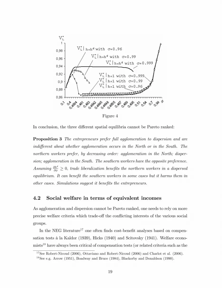
Figure 4
In conclusion, the three di¤erent spatial equilibria cannot be Pareto ranked:
Proposition 3 The entrepreneurs prefer full agglomeration to dispersion and are
indi¤erent about whether agglomeration occurs in the North or in the South. The
northern workers prefer, by decreasing order: agglomeration in the North; disper-
sion; agglomeration in the South. The southern workers have the opposite preference.
Assuming @hd
@�� 0; trade liberalization bene�ts the northern workers in a dispersed
equilibrium. It can bene�t the southern workers in some cases but it harms them in
other cases. Simulations suggest it bene�ts the entrepreneurs.
4.2 Social welfare in terms of equivalent incomes
As agglomeration and dispersion cannot be Pareto ranked, one needs to rely on more
precise welfare criteria which trade-o¤ the con�icting interests of the various social
groups.
In the NEG literature17 one often �nds cost-bene�t analyses based on compen-
sation tests à la Kaldor (1939), Hicks (1940) and Scitovsky (1941). Welfare econo-
mists18 have always been critical of compensation tests (or related criteria such as the
17See Robert-Nicoud (2006), Ottaviano and Robert-Nicoud (2006) and Charlot et al. (2006).18See e.g. Arrow (1951), Boadway and Bruce (1984), Blackorby and Donaldson (1990).
19

sum of compensating or equivalent variations) because that approach has at least
two important drawbacks: 1) it may lead to inconsistent social judgments �e.g.,
cyclical rankings of alternatives; 2) the compensation tests have a dubious ethical
value, because either the compensation is paid and the Pareto criterion then su¢ ces
to reach a decision, or the compensation is not paid, the losers remain losers and
the mere possibility of compensation is a meager consolation to them. Moreover,
such criteria are typically biased in favor of the rich when income e¤ects raise the
rich�s willingness to pay.
We propose to try a di¤erent approach here, which is based on the following
reasoning. Consider a fully integrated economy with no transport costs. In such an
economy the price of manufactured products would be p = v�=(��1) for all varietiesand for all consumers, independently of the location of production and consumption.
We propose to consider that in such an economy it would be ethically acceptable to
compare individuals in terms of their nominal income, even when they have di¤erent
preferences, since all individuals would then face the same price vector in the market.
Underlying this approach is the view that di¤erent preferences are not in themselves
a reason to give di¤erent levels of purchasing power to individuals. In short, their
preferences are a private matter and social justice has to do with sharing the value of
resources fairly, not with how individuals spend their income over various goods.19
The second principle we want to invoke is the Pareto principle: If all individuals are
indi¤erent between two situations, the social evaluation should also deem the two
situations equivalent.
With these two basic principles, one can actually evaluate allocations of the non-
integrated economy as well. For each such allocation, it su¢ ces to �nd an allocation
in the integrated economy such that every agent is indi¤erent between the two
allocations. By the Pareto principle, the two allocations are equivalent. And by this
procedure, it su¢ ces to be able to evaluate allocations of the integrated economy
in order to be able to evaluate all sorts of allocations. This procedure implies that,
in a non-integrated economy, individuals will be compared in terms of �equivalent
19This liberal approach to social justice has been famouly defended by Rawls (1971) and Dworkin
(2000).
20

incomes�,20 namely, the incomes that, in an integrated economy, would give them
the same satisfaction as in the allocation under consideration. Since indirect utility
is computed, for an agent of type r; as
V = (�r)�r (1� �r)1��r
Y
P �r
(recall that pA = 1), one has
(�r)�r (1� �r)1��r
Y
P �r= (�r)
�r (1� �r)1��r~Y~P �r
, ~Y =Y
P �r~P �r :
Therefore, if ~P is the price index in the integrated economy (one then has ~P =
n1
��1v�=(� � 1) with n = 1=f), the equivalent income ~Y can be meaningfully com-
pared across individuals of di¤erent locations and di¤erent preferences. Note that
~Y is a correct representation of any given individual�s preferences, in the sense that
an individual prefers an allocation to another if and only if his equivalent income is
greater in this allocation.21
In general, interpersonal comparisons based on equivalent incomes are di¤erent
from those relying on utilities or on real incomes. For two types of agents r and r0;
one has:
~Yr~Yr0
=VrVr0
(�r0)�r0 (1� �r0)1��r0
(�r)�r (1� �r)1��r
~P �r
~P �r0
=Yr=P
�r
Yr0=P �r0
~P �r
~P �0r:
In the case when all individuals have the same preferences (same parameter �r),
equivalent income is simply proportional to indirect utility V and to real income
Y=P �r : Therefore this approach is consistent with the widespread practice of rely-
ing on real incomes for interpersonal comparisons,22 but only when preferences are
identical. Besides, when all individuals face the reference price ~P one simply has
~Y = Y and nominal incomes can be used for comparisons.
Replacing P by its value in any equilibrium, one computes:
20More on the analytical, historical and philosophical underpinnings of this approach can be
found in Fleurbaey and Hammond (2004), Fleurbaey and Mongin (2005), Fleurbaey (2007).21It corresponds to a particular case of money-metric utility function (Samuelson 1974).22See, for instance, Charlot et al. (2006).
21

eY =Y
(h+ �h�)�r=(1��)in the North,
eY =Y
(�h+ h�)�r=(1��)in the South.
Then the equivalent incomes of the various kinds of agents are computed as follows:
ew =w
(h+ �h�)�h=(1��); ew� = w�
(�h+ h�)�h=(1��);
ewL =1
(h+ �h�)�L=(1��); ew�L = 1
(�h+ h�)��L=(1��)
:
In Figure 4 we analyse how these equivalent incomes vary with the number of
entrepreneurs in the North under di¤erent value of trade freeness.23
Figure 5
23Parameters: �h = 0:6; � = 3; � = 0:99; � = 1 and L = 2:4. Stable equilibria are represented
by black rounds.
22

When trade is relatively free (� = 0:9), the agglomerated equilibrium emerges and
this situation is detrimental for southern immobile workers. For a lower level of
trade freeness agglomeration is still a stable equilibrium in the North only (� =
0:34) or in the North and in the South (� = 0:3441). However for such a level
of trade freeness, the partial dispersion of activities also holds which improves the
equivalent income of southern workers and reduces that one of northern workers
(when agglomeration is initially located in the North). Lastly around autarky the
dispersed equilibrium is stable, and this situation is approximately the best for the
worst o¤. Why "approximately"? Because even in that case, southern workers
get a lower equivalent income than northern workers, activities are still too much
agglomerated from the point of view of the worst-o¤. In fact, depending on the
parameters, the dispersed equilibrium may favor the northern or southern workers.
For instance, assume that � = :1; � = 1:05, � = 3; �h = :6: Then, for � = :9; one
has ewL = ew�L for h = :519 while the dispersed equilibrium is hd = :531 (too much
agglomeration); for � = :95; one has ewL = ew�L for h = :509 while the dispersed
equilibrium is hd = :501 (too little agglomeration).24
Proposition 4 In the case of agglomeration, the worst-o¤ workers would prefer a
dispersed equilibrium. In the case of partial dispersion, the market may deliver too
much or too little agglomeration for the worst-o¤ workers.
In the Appendix, we show that a similar result holds when the upper-tier utility
is a logarithmic quasi-linear function.
5 Concluding remark
It is often argued that globalization leads to a reduction in taste diversity. In
the present work, we have shown that the reduction in taste heterogeneity fosters
24Note that when � = 1:05; an allocation of activities in proportion to the worker populations
would have h = :488: On the basis of simulations we conjecture that for � = 1 (equal populations
of workers in the two regions), the market equilibrium always displays too much agglomeration
from the point of view of the worst-o¤ workers.
23

multiple equilibria, which may be good news for peripheral under-developed regions
if this means that dispersed equilibria have greater chance of resisting the in�uence
of liberalization.
We have proposed a methodology to conduct welfare analysis in the presence of
heteregeneous tastes, and observed that market agglomeration is typically detrimen-
tal to the worst-o¤, although in the case of partial dispersion the market equilibrium
can be too much or too little dispersed in the eyes of the worst-o¤. Such conclu-
sions suggest that policy interventions are warranted in order to alleviate the welfare
consequences of the socially suboptimal spatial con�guration generated by market
forces. We did not take stand, however, on the degree of inequality aversion which
should guide such policies. A speci�c axiomatic analysis of the social ordering might
help obtain a more precise criterion. We leave this for another research. We hope
that the measure of welfare that has been proposed in this paper is at least useful
in mapping out the social consequences of market equilibria.
A Spatial equilibria and welfare with a quasi-linear
demand
Ottaviano et al. (2002) and P�üger (2004) propose models without income e¤ect,
indeed in the former the upper-tier utility is a quadratic quasi-linear function while
in the latter the upper-tier utility is a logarithmic quasi-linear function. We propose
here to study this last function with the same taste heterogeneity as in the text:
U = �r lnM + A r 2 fL;L�; hg:
Then we get:
cri =�rP 1��
p��i ;
Vh = ��h lnP + Y + (�h(ln�h � 1)):
24

The supply side is not modi�ed (q = (�� 1)fw=vwA) thus we get:
P 1�� =
�h+ �h�
f
�p1��; (P �)1�� =
��h+ h�
f
�p1��;
w =1
�
��hh+ �LL
h+ �h�+ �
�hh� + ��LL
�
�h+ h�
�:
Migration is now driven by the following equation:
Vh � V �h = �h ln(P �=P ) + (w � w�):
In order to keep the analysis as simple as possible, we assume that L = L� (i.e.
� = 1). Sustain points are given by:
�s =��
p�2 + 4L�(1 + L�)(�� 1)2�2(1 + L�)(1� �) ;
�s� =�+
p�2 + 4L�(1 + L��)(�� 1)22(1 + L��)(�� 1) :
Then � has the same impact on sustain points as �, an increase in it increases �s
and reduces �s�.
25

Figure A
However a di¤erence exists between these two kinds of taste heterogeneity, indeed
a decrease in � (compare Figure25 A.1 and A.3) generates an upward translation of
the relative real wage, which makes the symmetric equilibrium unstable (see Figure
A.2), while a decrease in � (with � = 1) makes the dispersed equilibrium stable for
a wider range of trade costs (see Figure A.4).
In order to perform welfare analysis based on equivalent income on the P�uger
model with taste heterogeneity, we plot Figure A.5.
Figure A.5
When trade costs are high or low, the results found are very similar to those obtained
in the text. Indeed in Figure A.526, we can observe that agglomeration and partial
25Parameters: �h = 0:3; � = 6; f = 1 and L = 1.26Parameters: �h = 0:5; � = 3; f = 0:5; L = 2:6 and � = 1.
26

dispersion are detrimental to southern immobile workers in term of equivalent in-
come in the case of a northern agglomeration. When the agglomerated equilibrium
in the South is chosen, the poorest people are located in the North and there is over
agglomeration in the South from their point of view. Having said that a new result
is found for intermediate trade freeness: indeed in that case the partial agglomer-
ation in the region where individuals have the weaker preference for the industrial
goods is the best stable outcome for the worst o¤. However dispersion is still the
unattainable (i.e., unstable) optimal equilibrium in the light of egalitarian principles.
References
Atkinson, A. B. (1970) On The Measurement of Inequality, Journal of Economic
Theory 2, 244-263.
Arrow K.J. (1951) Social Choice and Individual Values, New York: Wiley. 2nd
ed., 1963.
Baldwin, R.E., Forslid, R., Martin, R., Ottaviano, G.I.P., and F. Robert-Nicoud
(2003) Economic Geography and Public Policy, Princeton University Press, Prince-
ton NJ USA.
Blackorby C. and D. Donalson (1990) A review article: The case against the use
of the sum of compensating variations in cost-bene�t analysis, Canadian Journal of
Economics 23, 471-494.
Boadway R. and N. Bruce (1984) Welfare Economics, Oxford: Basil Blackwell.
Candau F. (2008) Entrepreneurs�Location Choice and Public Policies, a Survey
of the New Economic Geography. Journal of Economic Surveys, Vol. 22, Issue 5,
pp. 909-952.
Candau F. (2009) Is Agglomeration Desirable? SSRN working paper series
Charlot S., Gaigné C., Robert-Nicoud F. and J-F. Thisse (2006) Agglomeration
and Welfare: the core-periphery model in the light of Bentham, Kaldor, and Rawls,
Journal of Public Economics 90, 325-47.
Fleurbaey M. (2007) Social choice and just institutions: New perspectives. Eco-
nomics and Philosophy 23, 15-43.
27

Fleurbaey M., P.J. Hammond (2004) Interpersonally comparable utility. In S.
Barbera, P.J. Hammond, C. Seidl eds., Handbook of Utility Theory, vol. 2, Dor-
drecht: Kluwer.
Fleurbaey M., P. Mongin (2005) The news of the death of welfare economics is
greatly exaggerated. Social Choice and Welfare 25, 381-418.
Fleurbaey M., K. Suzumura and K. Tadenuma 2005, Arrovian aggregation in
economic environments: How much should we know about indi¤erence surfaces?,
Journal of Economic Theory, 124: 22-44.
Forslid R. and G.I.P. Ottaviano (2003) An Analytically Solvable Core-Periphery
Model, Journal of Economic Geography 3, 229-240.
Gaigné, C. (2006) The �genome�of Neg models with vertical linkages. A comment
on the welfare analysis. Journal of Economic Geography 6, 141-159.
Hicks J.R. (1939) The foundations of welfare economics, Economic Journal 49,
696-712.
Kaldor N. (1939) Welfare propositions and interpersonal comparisons of utility,
Economic Journal 49, 549-552.
Krugman P. (1980) Scale Economies, Product Di¤erentiation, and the Pattern
of Trade. The American Economic Review 70, 950-59.
Krugman P. (1991) Increasing Returns and Economic Geography, Journal of
Political Economy 99, p. 483-499.
Krugman P. and A. Venables (1995) Globalization and the inequality of nations,
Quarterly Journal of Economics 110, 857-880.
Murata Y. (2003) Product diversity, taste heterogeneity, and geographic distrib-
ution of economic activities: Market vs. non-market interactions, Journal of Urban
Economics 53, 126�144.
Murata Y. (2007) Taste heterogeneity and the scale of production: Fragmenta-
tion, uni�cation, and segmentation, Journal of Urban Economics, in press.
Ottaviano G.I.P (2002) Models of new economic geography: factor mobility
versus vertical linkages. Graduate Institute of International Studies, miméo.
Ottaviano G.I.P. and J.-F. Thisse (2002) Integration, agglomeration and the
political economics of factor mobility, Journal of Public Economics 83, 429-456.
28

Ottaviano G.I.P., T. Tabuchi and J-F. Thisse (2002) Agglomeration and trade
revisited, International Economic Review 43, p. 409�435.
Ottaviano G.I.P. and F. Robert-Nicoud (2006) The �genome�of NEG models
with vertical linkages: A positive and normative synthesis, Journal of Economic
Geography 6, p 113-39.
Pazner E. and D. Schmeidler (1978) Egalitarian equivalent allocations: A new
concept of economic equity, Quarterly Journal of Economics 92, 671-687.
P�üger M. (2004) A simple, Analytically Solvable Chamberlinian Agglomeration
Model, Regional Science and Urban Economics 34: 565-573.
P�üger, M., Südekum J. (2006.a) Towards a Unifying Approach of the �New
Economic Geography�IZA working paper No. 2256.
P�üger, M., Südekum J. (2006.b) Integration, agglomeration and welfare, Jour-
nal of Urban Economics in press.
Robert-Nicoud F. (2006) Agglomeration and trade with input-output linkage and
capital mobility. Spatial Economic Analysis (�rst issue), 101-126.
Samuelson P.A. (1974) Complementarity: An essay on the 40th anniversary of
the Hicks-Allen Revolution in Demand Theory. Journal of Economic Literature 12,
1255-1289.
Scitovsky T. (1941) A note of welfare propositions in economics, Review of Eco-
nomic Studies 9, 77-88.
Tabuchi, T. and J.-F. Thisse (2002) Taste heterogeneity, labor mobility and
economic geography, Journal of Development Economics 69, 155�177.
Zeng D.Z. (2007) New economic geography with heterogeneous preferences: An
explanation of segregation, Journal of Urban Economics in press.
29


