Embed Size (px)
Citation preview

Agricultural Price Distortions, Poverty and
Inequality in the Philippines
Caesar B. Cororaton Virginia Polytechnic Institute and State University
Erwin Corong International Food Policy Research Institute
John Cockburn Laval University
Agricultural Distortions Working Paper 101, June 2009 This is a product of a research project on Distortions to Agricultural Incentives, under the leadership of Kym Anderson of the World Bank’s Development Research Group. The authors are grateful to Kym Anderson, Thomas Hertel, Will Martin, Ernesto Valenzuela, Dominique van der Mensbrugghe and workshop participants for helpful comments, and for funding from World Bank Trust Funds provided by the governments of Japan, the Netherlands (BNPP) and the United Kingdom (DfID) and from the Poverty and Economic Policy (PEP) research network which is financed by the Australian Aid Agency, the Canadian International Development Agency and the International Development Research Centre. This paper will appear in Agricultural Price Distortions, Inequality and Poverty, edited by K. Anderson, J. Cockburn and W. Martin (forthcoming 2010). This is part of a Working Paper series (see www.worldbank.org/agdistortions) that is designed to promptly disseminate the findings of work in progress for comment before they are finalized. The views expressed are the authors’ alone and not necessarily those of the World Bank and its Executive Directors, nor the countries they represent, nor of the institutions providing funds for this research project.

1
Abstract
This paper analyzes the poverty and inequality implications of removing agricultural and
non-agricultural price distortions in the domestic market of the Philippines and abroad.
Liberalization in the rest of the world is poverty and inequality reducing, whereas full
domestic liberalization increases national poverty and inequality. Poverty declines while
inequality increases marginally in the combined scenario of both global and domestic
agriculture reform. Although the reduction in the national poverty headcount is small in the
latter scenario, the poorest of the poor – particularly those living in the rural areas – emerge
as “winners”, given their strong reliance on agricultural production and unskilled labor
wages.
JEL codes: D30, D58, D63, F13, O53, Q18
Keywords: Poverty, Agricultural Trade, Trade Liberalization, the Philippines
Author contact details:
Caesar B. Cororaton
Research Fellow
Global Issues Initiative (GII)
Institute for Society, Culture and Environment (ISCE)
Virginia Polytechnic Institute and State University
Alexandria VA

Agricultural Price Distortions, Poverty and
Inequality in the Philippines
Caesar B. Cororaton, Erwin Corong and John Cockburn
The Philippine agricultural sector employs 36 percent of the labor force and accounts for
roughly 14 percent of the nation’s Gross Domestic Product (GDP). When the agricultural-
based food processing sector is included, the whole of agriculture and food contributes 26
percent to GDP. From the 1950s to the 1970s, government policies were biased against
agriculture. These policies included the government’s import substitution policy until the
1980s which created a bias in favor of manufacturing and penalized returns to agricultural
investments and exports, export taxes and exchange rate over-valuation which greatly
reduced earnings from agriculture, and government intervention through the creation of
government corporations that siphoned off the gains from trade (Intal and Power 1990, David
2003). Then the trade reform program in the 1980s led to a shift from taxing to protecting
agriculture relative to non-agricultural sectors, and these policies became more pronounced
when the country became a member of the World Trade Organization (WTO) in 1995. As a
result, the current system of protection favors agriculture with both applied tariff rates and
nominal rates of assistance to agriculture substantially higher than for manufacturing (Aldaba
2005, David, Intal and Balisacan 2009). However, two decades of protection have failed to
induce competitiveness and productivity growth in agriculture.
This chapter analyzes what the poverty and inequality implications would be of
removing agricultural and non-agricultural price distortions in the domestic markets of the
Philippines, and also in markets abroad. The analysis uses results from ‘rest of the world
trade liberalization’ simulations from the global LINKAGE model1 of the World Bank (see
Anderson, Valenzuela and van der Mensbrugghe 2010) as exogenous shocks, along with
national liberalization shocks, to derive effects based on the Philippine computable general
equilibrium (CGE) model of Cororaton and Corong (2009). The global model incorporates 1 In this paper, the LINKAGE model (van der Mensbrugghe 2005) is also referred to as the global model. Both terms are used interchangeably.
2
new estimates of agricultural protection/assistance for various developing countries including
the Philippines,2 and simulates scenarios involving full world trade liberalization in all
sectors and in agriculture only. The global simulations generate changes in export and import
prices for the Philippines at the border, as well as changes in world export demand for
Philippine products.3 These results, together with the new estimates of protection/assistance
from David, Intal and Balisacan (2009) for the Philippines, are applied as shocks to the
Philippine CGE model in order to analyze the distributional, welfare and poverty impacts of
various trade liberalization scenarios for the country.
We conduct our simulation analysis in stages to assess the differing impacts that
international markets and domestic market liberalization may entail. In the first stage, we use
the changes in the border export and import prices and the changes in the world export
demand for Philippine products from the global model into the Philippine model without
altering the existing trade protection system in the country. In the second stage, we simulate
unilateral trade liberalization in the Philippines without incorporating any changes from the
global model. Finally, we combine the rest of the world with the unilateral liberalization
shocks to assess their total effects.
Six policy experiments are conducted, with separate scenarios for trade liberalization
in all sectors as compared with in agriculture sectors only. The agriculture sector is defined
here to include primary agriculture and lightly processed food.4 In each scenario, we generate
results at the macro and sectoral level as well as vectors of changes in household income,
consumer prices and sectoral employment shares. The latter three are then used as inputs into
a micro-simulation procedure to calculate the impact on poverty and inequality. The latter
draws on data from a national household survey conducted in 2000.
The chapter is organized as follows. The next section sheds light on the degree of
price distortions and trade protection as well as poverty trends in the Philippines. The
following section presents the structure of the Philippine CGE model, which is based on the
national social accounting matrix (SAM) as of 2000. The policy experiments and the results
2 Estimates of agricultural protection/assistance for the Philippines, based on David, Intal and Baliscan (2009), are incorporated in the World Bank’s global agricultural distortions database (Anderson and Valenzuela 2008). Those estimates cover five decades, but the representative values for CGE modeling as of 2004 that are used here are available in Valenzuela and Anderson (2008). 3 These vectors of changes are generated by simulating the global model with no Philippine trade liberalization. 4 This definition is maintained throughout the study. Agriculture is defined as primary agriculture (excluding fishing, forestry and agricultural services) and lightly processed food, while non-agriculture refers to all other sectors including highly processed foods, tobacco and beverages.

3
are then discussed, before the final section provides a summary of findings and some policy
implications.
Philippine trade and assistance policies and poverty trends
In 1949, the Philippines embarked on a development strategy geared towards industrial
import substitution with lesser emphasis on the agricultural and export sectors. It provided
protection to domestic producers of final goods with high tariff rates on non-essential
consumer goods and low tariffs on essential producer inputs. However, this policy did not
accomplish much, as the growth of manufacturing value added and industrial employment
increased minimally. In 1970, the government shifted towards export promotion, with tax
exemptions and fiscal incentives given to capital intensive firms located in export processing
zones. However, this strategy also achieved very little, as the highly skewed structure of tariff
protection in favor of import-substituting manufactured goods remained. Moreover, the
imposition of export taxes, the policy of keeping an over-valued exchange rate, and the
presence of government corporations which not only regulated domestic prices but also
siphoned off gains from domestic and international trade, created a strong bias against
agriculture and exports.
The restrictive trade policies adopted between the 1950s and the late 1970s that
prevented efficient resource allocation and smooth functioning of markets penalized the
domestic economy in three respects. First, import controls resulted in an over-valued
exchange rate that favored import-substituting firms. Second, continued protection increased
domestic output prices which impeded forward linkages. Third, tariff escalations and import
controls weakened backward linkages as tariffs on capital and intermediate goods were kept
low relative to finished products (Austria and Medalla 1996). This policy also promoted rent-
seeking activities and distorted economic incentives on investments in agriculture. The
agricultural sector, which served as the country’s backbone in providing the necessary
foreign exchange needed by the import-dependent manufacturing sector, stagnated while the
industrial sector ventured into import-dependent assembly operations with minimal value-
added content and little or no forward and backward linkages.
Realizing the pitfalls of the import-substitution policy followed by an unsuccessful
export-promotion strategy, the government implemented a series of trade reform programs

4
(TRP) starting in 1981.5 The Philippines also has participated more actively in the
multilateral trading system since it joined the World Trade Organization (WTO) in 1995. For
example, between 1995 and 1999 the country complied with all of its multilateral
commitments within the prescribed timeframes (WTO 1999). These commitments included
tariff bindings at a maximum of 10 percentage points over the year 1995 applied rate on
roughly 65 percent of all tariff lines, tariff bindings on selected information technology
products, and binding of market access in selected services sectors (Austria 2001). Even so,
there continues to be a substantial tariff binding overhang, especially in agriculture.6
By the turn of the century, the country slowed down its pace of trade reforms (WTO
2005). Although the average applied Most Favored Nation (MFN) tariff rate declined from
9.7 to 5.8 percent between 1999 and 2003, it then rose to 7.4 percent in 2004. This reversal of
the tariff adjustment process was brought about by presidential discretion, aimed at helping
problematic domestic industries and responding to lobbying from domestic interest groups.
Estimates of nominal rate of assistance to agriculture
David, Intal and Balisacan (2009) recently estimated the nominal rate of assistance (NRA) to
key industries in the agricultural sector. The NRA is the percentage difference between the
domestic and the border price and thus measures how policy-induced distortions directly
affect producer incentives. The NRA for coconut (copra or dried coconut) is negative
throughout the years shown in Table 1, largely due to export taxes, a coconut levy, and a
copra export ban. The currency devaluation in the 1970s and the world commodity boom in
the middle of that decade did not translate into higher profits for coconut farmers, but rather
to higher revenue for the government and lower raw material costs for the coconut oil milling
industry. Although these policies began to be eliminated from 1986, coconut farmers remain
penalized owing to the continued existence of a government corporation which controls 70-
80 percent of coconut oil milling, thereby retaining a monopsonistic command over domestic
price of copra.
The NRA for corn has always been positive and exhibits an increasing trend. There is
not much political pressure on corn compared to rice because it is a subsistence crop for
5 The TRPs were major components of the structural programs prescribed by multilateral agencies (including the World Bank and International Monetary Fund) in the 1980s. The Philippines is currently on the fourth phase of its TRP. See Cororaton, Cockburn and Corong (2006) for a detailed discussion. 6 Tariff binding overhang refers to the difference between a country’s bound tariffs (tariff rates which a country commits in the WTO not to exceed) and its applied tariffs.

5
upland farmers in the Southern part of the country. Nonetheless, it is also a major animal feed
ingredient. Among agricultural crops, sugar has had the highest NRA since the 1960s. There
was a shift in the burden of protection from United States’ consumers in the 1960s and early
1970s when a major part of domestic production was exported to the United States market
through an export quota to Filipino producers and food processors (known as the Laurel-
Langley Agreement). This agreement ended in 1974, resulting in a dramatic drop in
Philippine sugar exports to the United States.7
The NRA for chicken has been consistently high and well above that for pork.
However, the government imposed the same level of in-quota and out-of-quota tariffs for
both commodities after the ratification of the WTO agreement in 1995. On the other hand,
cattle were not included as part of Philippines’ sensitive products list in the WTO. Hence,
cattle’s NRA has been low compared to chicken and pork. In the early 1990s, the government
attempted to promote cattle fattening activities and allowed duty-free imports of young cattle
while at the same time imposing more restrictive non-tariff barriers on beef. Nevertheless,
cattle fattening activities did not prosper as tariffs on beef fell.
Before the mid-1980s, the NRAs for agricultural inputs such as fertilizer, agricultural
chemicals and farm machinery were generally higher than the NRAs for agricultural crops,
averaging well above 20 percent (David, Intal and Baliscan 2009). This was largely due to
the government’s industrial promotion policies that increased domestic prices of
manufactured inputs to agriculture. However, after this period and during the trade
liberalization process there were substantial reductions in agricultural input protection, down
to around 10 percent in the latter 1990s and to a uniform 3 percent in 2000-04.
Poverty trends
In both rural and urban areas, over 60 percent of the expenditure of poor households is on
food, of which almost half is on cereals, primarily rice and corn (Table 2). Rural dwellers
spend proportionately more on food than their urban counterparts. Food consumption among
non-poor households is somewhat less (38 8 percent), with urban non-poor households
spending the least amount on food and cereals (8 percent).
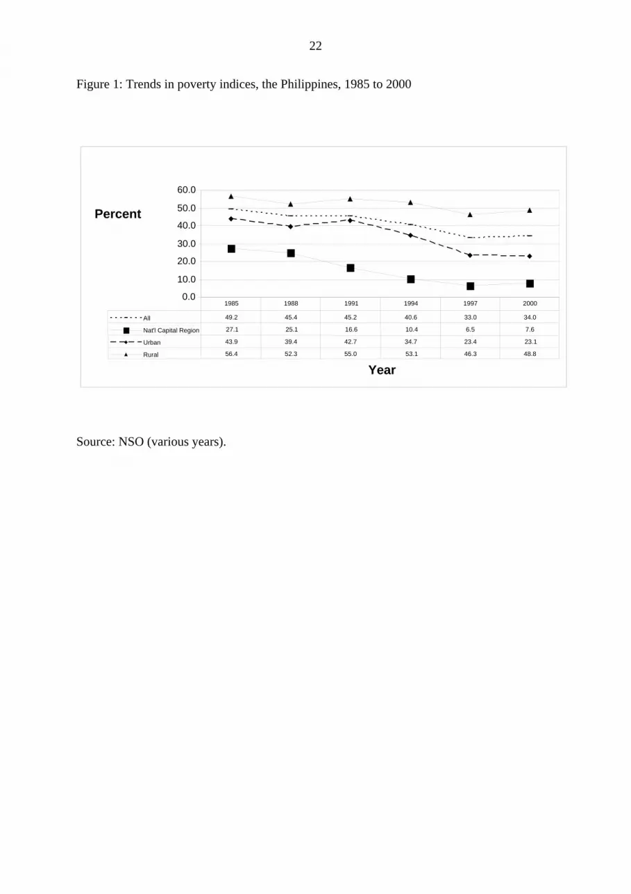
Figure 1 presents the evolution of the poverty headcount index between 1985 and
2000. The national headcount index decreased from almost 50 percent to roughly 34 percent
over that period. However, this fall was mainly concentrated in urban areas, especially in the 7 Sugar exports accounted for only 10 percent of domestic production during this period.

6
National Capital Region where poverty was already low. In contrast, the rural headcount
index fell only modestly, from 56 to 49 percent as compared with the fall from 44 to 23
percent for urban areas.
The CGE model
The national CGE model used in this study8 is calibrated to the year 2000 Social Accounting
Matrix (SAM) of the Philippines.9 There are 41 production sectors and four factors: two labor
types (skilled workers with at least a college diploma, and unskilled) plus capital and land.
Institutions include the government, firms, households and the rest of the world. Household
categories are defined by income deciles. Output (X) is a composite of value added (VA) and
intermediate inputs. Output is sold either to the domestic market (D) or to the export market
(E) or both. The model assumes perfect substitutability between E and D. A finite elasticity
of export demand is assumed. Domestic market supply comes from two sources, domestic
output and imports (M), with substitution between D and M depending on the changes in
relative prices of D and M and on a constant elasticity of substitution (CES) function.
Sectoral output is a Leontief function of intermediate inputs and value added. Value
added in agriculture is a CES function of skilled labor, unskilled labor, capital and land. Non-
agricultural value added is also a CES function of the same factors except land. Capital and
land are each sector specific, skilled and unskilled labor are mobile across sectors but limited
within skill category, and land use is mobile within the agricultural sector.
Households earn their income from factors of production, transfers, foreign
remittances and dividends, while at the same time paying direct income tax to the
government. Household savings is a fixed proportion of disposable income and household
demand is represented by a linear expenditure system (LES).
Government revenue is the sum of direct taxes on household and firm income,
indirect taxes on domestic and imported goods, and other receipts. The government spends on
consumption of goods and services, transfers and other payments. In the present version of
the model, we assume a fixed government balance. Since shifts in policy will result in
8 The specification of the model is based on “EXTER” (see Decaluwé, Dumont and Robichaud 2000). For a complete discussion and specification of the model, see Cororaton and Corong, 2009. 9 See Cororaton and Corong (2009) for details on the SAM construction.

7
changes in government income and expenditure, the government balance is held fixed
through a tax replacement variable. For the present analysis we use an indirect tax
replacement on domestic sales, but we also compare the results with the effects under a direct
tax replacement on household income. Either way, the tax replacement is endogenously
determined so as to maintain a fixed government balance level.
Foreign savings are held fixed. The nominal exchange rate is the model’s numéraire.
We introduce a weighted price of investment and derive total investment in real prices, which
is held fixed by introducing an adjustment factor in the household savings function. The
equilibrium in the model is achieved when supply of and demand for goods and services are
equal and investment is equal to savings.
Table 3 presents the production structure in the SAM. Generally, agricultural and
service sectors have higher value added shares (as a percent of output) compared to the
industrial sector. In agriculture, coconut and forestry have the highest value added shares of
almost 90 percent, while petroleum refining has the lowest among industrial sectors at 14
percent. The capital-output ratio in agriculture is generally lower than in industry and service
sectors. The largest employer of labor is the service sector. More than 90 percent of labor
input into agricultural production is unskilled labor. The share of skilled labor employed in
the industrial sector is substantially higher compared to the agricultural sector. The structure
of indirect tax reveals that tobacco and alcohol followed by petroleum have the highest
indirect tax, with 23 and 18 percent, respectively (last column of table 3).
Table 4 shows that almost 50 percent of exports come from electrical products. A
major part of this sector is the semi-conductor industry. Sizeable amounts of exports also
come from machinery and transport equipment. Almost 90 percent of the production of
electrical products is exported. The machinery and transport equipment industry also has a
high export intensity ratio, at 73 percent,10 followed by other manufacturing, coconut oil,
leather, fertilizer, other chemicals, garments, fruit processing, and fish processing. On the
import side, electrical products as well as machinery and transport equipment account for 35
and 12 percent of total imports, respectively, so these two sectors have high import intensity
ratios. Similar sectors where imports are a major source of domestic supply include other
crops, cattle, mining and crude oil, milk and diary, fruit processing, fish processing, coconut
oil, sugar milling, other food, textile, leather, paper, fertilizer, other chemicals, petroleum,
cement, and transportation and communication. 10 The export (import) intensity ratio is defined as the sector’s exports (imports) divided by its output (domestic supply).

8
Table 4 also shows the values of key elasticity parameters used in the model: the
import substitution elasticity (sig_m) in the CES composite good function, the production
substitution elasticity (sig_va) in the CES value added production function, and the export
demand elasticity (eta) which is obtained from the Armington parameter of the global model.
The consumption structure of households is presented in table 5. Rice is a significant
staple for Filipinos, especially among poorer households: it accounts for 14.3 of total
expenditure for the first decile of households, but its share decreases substantially as
households become richer. Fish and meat, fruits and vegetables, and other food are the other
significant items in household consumption. Generally, lower income groups have substantial
expenditure on food and food related products. For instance, food items accounts for 42.4 of
total expenditure for the first decile compared with 13.4 percent for the tenth decile. Richer
households spend more on services relative to poorer ones. Products of special interest are
corn, sugar, chicken, meat processing, milk and dairy, fruit processing, fish processing, rice
and corn milling, sugar milling. The share of expenditure on these special products declines
as we move to the higher decline: they account for 25 percent of consumption in the first
decile but only 8.6 percent in the tenth decile.
Simulations
All policy experiments reported in this study use an indirect tax replacement to maintain
fixed government balance. We generate results at the macro and sectoral level as well as
vectors of changes in household income, consumer prices and sectoral employment shares.
The latter three are then used as inputs in a micro-simulation procedure that calculates the
impact on poverty and inequality, based on year 2000 household survey. Sensitivity analysis
with alternative direct tax replacement schemes is also undertaken.
Definition of policy experiments
Table 6 shows the sectoral correspondence between the Philippine CGE and the global
model, as well as information on the sectoral tariff rates and export subsidies based on the
new estimates of nominal rate of protection/assistance for the Philippines. The Philippine
CGE model is initially solved using new these estimates of protection/assistance to serve as

9
the base from which all subsequent simulations are compared. In certain policy experiments,
the global simulation results from the LINKAGE model are used as policy shocks to the
Philippine model, following the method proposed by Horridge and Zhai (2006).
The six policy experiments are:
• ROW-ALL – Rest of the world (ROW) trade liberalization in all sectors,
excluding the Philippines. This experiment uses the results of the global model
under full ROW liberalization in Table 6 and retains all existing trade distortions
(tariff rates and export subsidies) in the Philippines.
• ROW-AGR – Rest of the world liberalization in agriculture and lightly processed
food only. As with ROW-ALL, we utilize the results of the global model except
just under ROW agriculture and lightly processed food liberalization, again with
all existing Philippine trade distortions being retained.
• PHIL-ALL – Unilateral trade liberalization in all sectors. All Philippine trade
distortions are eliminated. No changes in the sectoral border export and import
prices or in export demand are included in this unilateral liberalization.
• PHIL-AGR – Unilateral agriculture trade liberalization. All trade distortions in
primary agriculture and lightly processed foods in the Philippines are
eliminated. Similar to PHIL-ALL, there are no changes in the sectoral border
export and import prices or export demand in this unilateral liberalization.
• COMB-ALL – Full rest of the world and Philippine trade liberalization, that is,
ROW-ALL and PHIL-ALL combined to cause global liberalization.
• COMB-AGR – Rest of the world and Philippine liberalization in agriculture and
lightly processed foods. This scenario combines ROW-AGR and PHIL-AGR.

10
Results
In this section we present modeling results from the six policy experiments lists in the
previous section sequentially, and then report the impacts on household income and welfare
and then on poverty and inequality. The section concludes with some additional results that
show the sensitivity of the core results to changes in the treatment of tax adjustments in the
model.
Rest of the world trade liberalization in all sectors (ROW-ALL)
Results from the LINKAGE model in table 6 indicate that this first policy experiment leads to
higher export prices and export demand for Philippine products. Within agriculture, a
significant shift in export demand is observed among sugar milling as well as raw fruits and
vegetables (with 1.5 and 1.1 percent, respectively). This is also true for fruit and fish
processing (1.2 percent), whereas slightly more modest export demand shifts are observed in
other industrial and services sectors. At the same time, full ROW liberalization would lead to
higher world import prices for most Philippine goods.
Table 7 shows that overall export prices in local currency increase more in the
agricultural sectors than the non-agricultural sectors, by an average of 3.6 versus 2.4 percent.
So too do export volumes: they expand 9.8 percent for agriculture compared with a modest
0.3 percent rise for non-agricultural exports. Local import prices also increase more in
agriculture than in non-agriculture (3.0 versus 1.1 percent). Substitution towards imported
goods is observed owing to a larger increase in the price of domestically produced goods
relative to their imported counterparts. Because of this, agricultural and non-agricultural
import volumes increase by 0.9 and 1.1 percent, respectively (second column of table 7).
The entire agricultural sector benefits from the more-favorable international market
conditions. Agricultural output and value added prices increase by 3.5 and 3.9 percent,
respectively. Thus, returns to agriculture-specific factors, in particular land and agricultural
capital (which increase by 5.1 and 4.7 percent, respectively), rise relatively to wage rates (3
percent) and to the returns to non-agricultural capital (2.9 percent). Unskilled wage increase

11
slightly more than skilled wage, as unskilled workers are used more intensively in the
expanding agricultural sector.
By contrast, for non-agricultural sectors, the fall in domestic sales offsets export
expansion, such that the volume of output contracts by 0.1 percent. Essentially, this is
traceable to the import-domestic price substitution effects discussed earlier, the fall in world
import prices for essential consumer goods like garments (table 6), and the real exchange rate
appreciation. In spite of falling output volumes, non-agricultural output prices still increase
by 2.5 percent owing to higher export prices. Hence, returns to factors such as non-
agricultural capital and skilled workers, which are used intensively in non-agriculture,
increase as well.
Rest of the world trade liberalization in agriculture only (ROW-AGR)
The results of ROW-AGR scenario are similar but smaller in magnitude compared to ROW-
ALL. We will only focus on different results in this scenario since the mechanisms driving the
model results are essentially the same to ROW-ALL. Agricultural exports increase by 11
percent (table 7) mainly due to significant export demand shift in sugar, raw fruits and
vegetables (1.6 and 1.2 percent, respectively, in Table 6). A distinct feature of this scenario is
that domestic agriculture prices increase less than the rise in agricultural import prices (1.7
versus 2.7 percent). In the face of more expensive agricultural imports, domestic demand
expands while imports fall (0.1 and 1.2 percent, respectively). With this, agricultural output
expands as agricultural domestic demand account for a larger share of domestic agriculture
output.
The absence of non-agricultural liberalization results in a 0.1 percent decline in non-
agricultural exports, since most non-agricultural goods have little or no change in world
export demand (table 6). Non-agricultural imports rise while domestic demand declines (0.3
versus 0.1 percent), as domestic prices increase more relative to import prices (0.9 and 0.3
percent, respectively). The contraction in domestic demand together with the 0.1 percent
decline in exports leads to a 0.1 percent dip in non-agricultural output. Nonetheless, non-
agricultural output and value added prices still increase, owing to higher export and domestic
prices.

12
Full unilateral trade liberalization in the Philippines (PHIL-ALL)
This experiment eliminates all sectoral tariff rates and export subsidies in the Philippines and
assumes no changes from the global model. PHIL-ALL leads to a 7.2 and 2.1 percent decline
in the local price of imported agricultural and non-agriculture products, respectively (Table
7). Import prices fall more and import volumes correspondingly increase more in agriculture
than in non-agriculture, as the initial distortions were higher in agriculture. In the face of
cheaper imports relative to domestic prices, domestic demand declines for local agricultural
and non-agricultural producers. At the same time, they benefit from cost savings on their
imported inputs, resulting in 2.3 and 1.7 percent falls in the domestic cost of production in the
agricultural and non-agricultural sectors, respectively. The real exchange rate depreciates by
1.6 percent, making Philippine-made products relatively cheaper in the international market.
This, coupled with falling domestic prices in the face of cheaper imports and input cost
savings, encourages producers to reallocate resources towards the export market (table 7).
While exports rise for both agriculture and non-agriculture, domestic demand falls
more for agriculture. Since domestic demand represents a larger share in agricultural output,
agricultural output contracts while non-agricultural output expands. Output and value added
prices in both agriculture and non-agriculture fall, but the fall in the former is higher than in
the latter. The result of all these adjustments is a fall in all factor returns, with factors used
intensively in agriculture experiencing a much higher reduction: returns to agricultural capital
and land decline by 5.7 and 4.6 percent, respectively, whereas non-agricultural capital returns
fall by just 1.3 percent. Nominal wages for unskilled workers fall more relative to skilled
wages, as unskilled workers are used more intensively in the agricultural sector.
Unilateral agriculture only trade liberalization in the Philippines (PHIL-AGR)
Unilateral liberalization in agriculture and lightly processed food results in substantial
expansion in agricultural imports (17 percent) owing to the significant decline in local
agricultural import prices (7.9 percent). At the same time, the removal of domestic
agricultural distortions also generates cost savings for the export-oriented lightly processed
sector, given its reliance on primary agricultural inputs. Thus, agricultural industries, which
in the context of this study include lightly processed food processors, reorient their
production towards the export market, resulting in a 6.2 percent export expansion and a 2.8

13
percent reduction in domestic sales. The net result is a contraction in agricultural output,
since domestic sales comprise a larger share of total agricultural output. As a result,
agricultural value added and value added prices fall along with the returns to all agricultural
factors. Returns to land drop 3.5 percent, returns to agricultural capital decline by 4.5 percent,
and wages of unskilled workers fall by 1.2 percent.
The results for non-agricultural sectors are the opposite. Import prices increase
marginally by 0.1 percent while domestic prices fall by 0.7 percent, resulting in 0.2 percent
expansion in domestic sales. Domestic prices decrease more relative to world prices (0.7
versus 0.3 percent), leading to a 1 percent export expansion. This, together with higher
domestic demand, allows overall non-agricultural output to expand by 0.3 percent.
A comparison of the sectoral results between PHIL-ALL and PHIL-AGR in table 7
confirms the heavier price burden of agricultural protection on the Philippine economy.
Indeed, removing agricultural distortions account for at least two thirds of the price reduction
in export, import, domestic, output, value added and consumer price index.11 This is also true
for factor prices, where between 40 and 80 percent of the fall in factor returns is traceable to
the removal of agricultural protection.
Rest of the world and Philippine trade liberalization in all sectors (COMB-ALL)
This experiment combines both rest of the world and domestic trade liberalization. The ROW
trade liberalization impact dominates the unilateral trade liberalization effects for both
agriculture and non-agricultural sectors. Local import prices decline particularly in the
agricultural sector, in spite of the increase in world commodity prices, indicating the
substantial level of domestic distortions in the Philippines. Cheaper imports crowd out their
domestically produced counterparts leading to a contraction in domestic sales for domestic
producers, once again hitting the agricultural sector much harder than the non-agricultural
sector. At the same time, rising world export prices, real exchange rate depreciation and cost
savings on imported inputs allow domestic producers to successfully reorient a large share of
their production toward the more profitable export market. Given the greater reliance of the
agricultural sector on domestic sales, the net impact is a contraction in the agricultural sector
and an expansion of the non-agricultural sector. 11 Ratio of prices in PHIL-AGR relative to PHIL-ALL in Table 7: Export (-1.3/-1.8 = 0.7); Import (-7.9/-7.2 = 1.1); Domestic (-2.2/-2.3 = 1.0); Output (-2.3/-3.1 = 0.8); Value Added (-2.9/-4 = 0.7); Consumer price index (-1.1/-1.3 = 0.8); Skilled wage (-0.9/-1.6=0.4); Unskilled wage (-1.2/-2.5=0.5); return to land (-3.5/-4.7=0.7); return to agricultural capital (-4.5/-5.7=0.8); return to non-agricultural capital (-0.5/-1.3=0.4).

14
Output prices for both agriculture and non-agricultural sectors increase (0.4 and 0.9
percent, respectively), with the former experiencing a smaller increase owing to a substantial
level of domestic agricultural distortions in the base. All factor prices with the exception of
returns to agricultural capital increase especially for non-agricultural sectors, although by less
than in ROW-ALL. The output volume impacts are the opposite, with unilateral liberalization
dominating rest of the world trade liberalization effects. Thus, overall agricultural output
declines while overall output of non-agricultural sectors improves (-1.9 and 0.3 percent,
respectively).
Rest of the world and Philippine trade liberalization in agriculture only (COMB-AGR)
The unilateral agricultural trade liberalization (PHIL-AGR) scenario dominates global
agricultural trade liberalization (ROW-AGR). Output , price and volume in agriculture
decline, as do agricultural factor prices. Once again, local import prices in agriculture decline
in spite of rising world commodity prices, indicating the substantial level of domestic
distortions in the Philippines. The positive impact of higher world commodity prices is
dominated by the negative impact of domestic agricultural distortions imposed by the
government. Thus, returns to factors used intensively in agriculture (land, agricultural capital
and unskilled wages) fall in response to declining agricultural output prices.
By contrast, local import prices in non-agricultural sectors increase. This is expected
since the country’s non-agricultural trade distortions are already low relative to international
standards.12 Thus, the overall output price of non-agricultural products increases by 0.2
percent, resulting in an output expansion and consequently higher returns to non-agricultural
factors (Table 7).
Household income, consumer price index, and welfare
The changes in nominal household income, nominal consumer price indices (based on
household-specific consumer baskets) and real income/welfare are presented in Table 8. In
interpreting the changes in household-specific consumer prices, recall from above that
primary and processed food account for a significant share of household expenditure,
12 This is because the various previous rounds of trade reforms in the country primarily focused on reducing non-agricultural distortions.

15
especially for the lower income groups, and that both primary and processed food items have
higher initial tariff rates than other goods (tables 4 and 5).
ROW-ALL, the scenario of global trade liberalization in all sectors (excluding the
Philippines) registers the greatest increase in nominal household income, as rising world
prices translate into higher factor returns. For the same reason, consumer prices also increase
the most in this scenario. Nonetheless, the greater nominal income growth for all households
outweighs the detrimental effects of rising consumer prices, with the result that welfare
increases for all household groups. Income and consumer price variations tend to be higher
for the poorest deciles, which are more tightly linked to the agricultural sector and which post
generally better welfare results. The results under ROW-AGR are similar but less than half as
large. Results are qualitatively similar and again display a generally pro-poor effect (Table 8).
The two domestic liberalization scenarios (PHIL-ALL and PHIL-AGR) all result in
falling consumer prices, driven by the reduction in local import and export prices as the
Philippine’s own trade-related distortions are eliminated. This price reduction is greater when
(agricultural and non-agricultural) domestic liberalizations are combined. We see that
removing domestic agricultural distortions reduces consumer prices more than the removal of
non-agricultural distortions, given the high share of agriculture in household consumption
and their higher initial levels of protection. A comparison of changes in consumer prices for
scenarios PHIL-ALL and PHIL-AGR show that roughly 1.8 out of the 2.2 percent reduction in
the consumer price index of the first decile is due to the elimination of domestic agricultural
distortions alone (Table 8).
Also observe that nominal incomes fall under the two unilateral liberalization
scenarios. However, the consumer price effects dominate such that, despite falling nominal
incomes, welfare/real income increases more under agricultural trade liberalization.
Furthermore, these welfare gains accrue proportionately more to poorer deciles owing to their
higher agricultural consumption.
These welfare gains are further bolstered with ROW and unilateral trade liberalization
combined. Nominal income increases under the full ROW and domestic trade liberalization
scenario, but this is somewhat offset by soaring consumer prices. Overall, it is the combined
global and domestic agricultural trade liberalization (COMB-AGR) scenario that provides the
highest increase in welfare. This is because the nominal income gains from the rest of the
world trade liberalization are largely conserved and to which are added the consumer price
reductions from domestic trade liberalization. In this case, the poorest deciles emerge as the

16
“winners”, both due to domestic agricultural trade liberalization and the pro-agricultural
nature of rest of the world trade liberalization.
Effects on poverty and inequality
The micro-simulation process utilized in the present study13 makes use of the year 2000
family income and expenditure survey (FIES) of the Philippines (NSO 2000). In order
estimate the likely poverty and inequality impacts of labor market conditions arising from
trade liberalization, we use in a sequential manner certain information from the CGE model
and apply it as an input into the micro-simulation procedure. In particular, we use the vectors
of changes in total income of households; wage income, capital income and other income;
household specific consumer price indices to update the nominal value of the poverty line;
and sectoral employment shares.
The method we employ is to incorporate changes in the employment status of
households after the simulation through a random process. In this way, it is possible to
capture households/laborers moving in and out of employment (at the micro level) by taking
into account changes in sectoral employment arising from a policy shift (at the macro level).
For instance, households with no labor income, due to unemployment, may become
employed and consequently earn labor income. Similarly, employed households may become
unemployed and earn no labor income at all after the policy change. Household labor income
is affected by changes in wages as well as the chance of getting unemployed after the policy
shock. The micro-simulation process is repeated 30 times,14 allowing us to derive confidence
intervals15 on our Foster-Greer-Thorbecke (FGT) indices and Gini coefficient estimates.
In order to take advantage of the richness of the micro-simulation procedure, we
calculate poverty indices and Gini coefficients based on the demographic characteristics of
the household head: gender, skill level and location (urban or rural). In total, the final FGT
indices are derived for 8 categories of household heads. Using demographic characteristics
instead of income deciles to evaluate changes in poverty and income distribution is
preferable, because it allows for a better policy evaluation and identification of the gainers
and losers from trade liberalization.
13 This is a modified approach of the original version proposed by Vos (2005). 14 Vos (2005) observes that 30 iterations are sufficient, as repeating this process additionally does not significantly alter the results. 15 Results on confidence intervals are available from the contact author upon request.

17
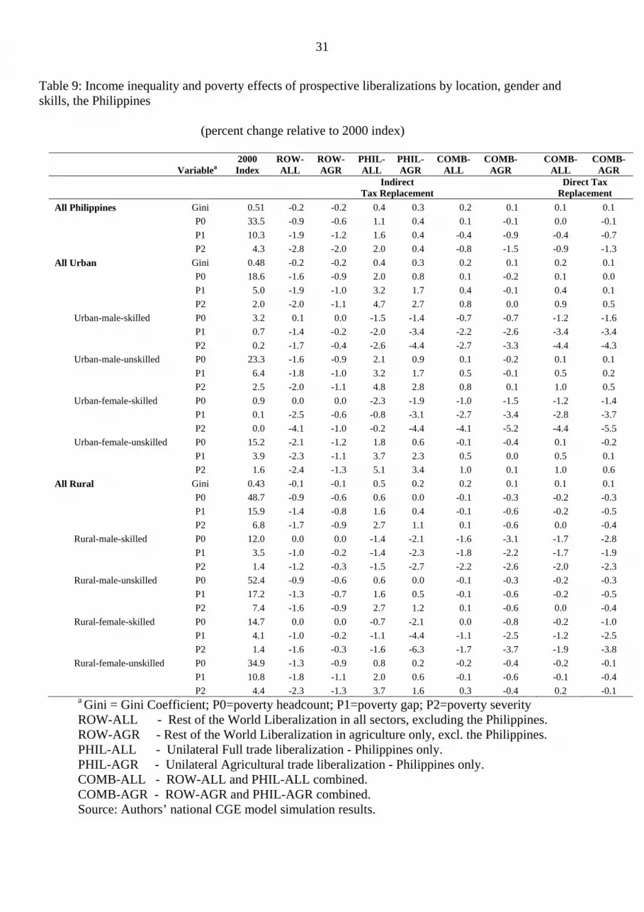
The poverty and inequality results in all experiments are summarized in Table 9.
Inequality marginally worsens in all unilateral liberalization scenarios, but slightly improves
in the ROW liberalization scenarios. The latter is due to the increase in nominal income
among poorer households while the former results from greater decrease in poorer
household’s nominal income relative to richer households (table 8).
Rest of the world liberalization reduces poverty at the national level and favors
unskilled households, as rising world demand and export prices for Philippine-made products
bring about higher agricultural factor returns (table 7). In contrast, unilateral liberalization
favors skilled households such that national poverty indices worsen. This is because the
removal of the Philippines’ own distortions results in resource reallocation towards outward
oriented and externally competitive non-agricultural sectors that employ skilled workers
intensively.
Poverty generally falls under the combined global and domestic liberalization
scenario, with the poverty reducing impact of ROW liberalization dominating the poverty
increasing effect of unilateral liberalization. In contrast, inequality marginally rises with the
inequality increasing effect of unilateral liberalization dominating the inequality reducing
effect of ROW liberalization. The combined global and domestic agricultural reform is the
most poverty friendly scenario. Although the national poverty headcount decreases
marginally, all household groups with the slight exception of urban households headed by an
unskilled worker share in the benefits from the poverty friendliness of trade liberalization.
Indeed, the poorest of the poor particularly those residing in the rural areas emerge as
“winners”, because of their reliance on agricultural production and wages unskilled labor.
These results are consistent with those obtained by Cororaton, Cockburn, and Corong
(2006). However, their results suggest a worsening of both the poverty gap and severity of
poverty while the current results find the opposite, especially under the combined ROW and
Philippine agricultural liberalization. This difference is traceable to the use of more-recent
estimates of trade protection on key food items (such as rice, corn, sugar and processed meat)
which, when eliminated, result in a significant fall in consumer prices faced by lower-income
groups (table 7).
Sensitivity analysis: indirect and direct tax replacement
18
The results discussed above are derived using indirect tax replacement. Are the results
sensitive to the tax replacement used? This section compares the above results with those
when a direct tax replacement closure is adopted. We focus on analyzing the poverty and
inequality results of COMB-ALL (full ROW and domestic trade liberalization) and COMB-
AGR (ROW and domestic agriculture trade liberalization).
The sensitivity analyses are presented in Table 9. The directions of change in poverty
indices and inequality are generally the same regardless of the tax replacement scheme.
However, the magnitudes are marginally higher under the direct tax scenario, owing to lesser
increase in consumer prices since direct taxes are used to compensate for foregone tariff
revenues.
Summary and policy implications
Starting in the 1980s, the government shifted from taxing to protecting agriculture relative to
non-agricultural sectors. However, two decades of protection failed to induce competitiveness
and productivity growth as agriculture became inward looking and inefficient. This study
analyzed the poverty and inequality implications of removing the agricultural and non-
agricultural price distortions as of 2004 in the domestic markets of the Philippines, and
compared those effects with what would happen if policies abroad were to be liberalized.
Rest of the world liberalization (ROW) reduces poverty at the national level and
favors unskilled households in the Philippines, as higher world export prices and export
demand for Philippine-made products allow Filipino producers to benefit from favorable
international market conditions. Nominal income improves significantly, outweighing the
impact of higher consumer prices. ROW trade liberalization in all sectors generates almost
uniform increases in real incomes across household types, while ROW trade liberalization in
agriculture brings about progressive changes in real income that benefit lower-income groups
more.
Unilateral trade liberalization leads to falling consumer prices, driven by the reduction
in local import and export prices as the Philippine’s own trade-related distortions are
eliminated. Import prices fall more and import volumes correspondingly increase more in
agriculture than in non-agriculture, as the initial distortions are higher in agriculture.
However, unilateral liberalization favors skilled households such that national poverty indices

19
and inequality worsen. This is because the removal of the Philippines’ own distortion results
in resource reallocation towards outward-oriented and externally competitive non-agricultural
sectors that employ skilled workers intensively.
The combined global and domestic agricultural reform appears to be the most poverty
friendly scenario for the Philippines. Although the national poverty headcount decreases only
marginally, all household groups with the slight exception of urban households headed by an
unskilled worker share the benefits from the poverty friendliness of that trade liberalization.
The poorest of the poor – particularly those living in the rural areas – emerge as “winners”,
given their reliance on agricultural production and wages from unskilled labor. Thus, taking a
pro-active trade liberalization stance, by fully participating with the rest of the world in trade
liberalization efforts through including its own domestic liberalization appears to be in the
best interests of the Philippines. Sensitivity analysis confirms that the results are not affected
by differing tax replacement assumptions, as a similar pattern of effects emerge regardless of
whether indirect or direct tax replacements are used.
References
Aldaba, R. (2005), “Policy Reversals, Lobby Groups, and Economic Distortions”, PIDS
Discussion Paper No. 2005-04, Philippine Institute for Development Studies (PIDS),
Makati.
Anderson K. and E. Valenzuela (2008),’Estimates of Global Distortions to Agricultural
Incentives, 1955 to 2007’, World Bank, Washington DC, October, accessible at
www.worldbank.org/agdistortions.
Anderson, K., E. Valenzuela and D. van der Mensbrugghe (2010), “Global Poverty Effects of
Agricultural and Trade Policies Using the Linkage Model”, Ch. 2 in K. Anderson, J.
Cockburn and W. Martin (eds.), Agricultural Price Distortions, Inequality and Poverty,
London: Palgrave Macmillan and Washington DC: World Bank.
Austria, M. (2001), “Liberalization and Regional Integration: The Philippines’ Strategy for
Rest of the World Competitiveness”, Philippine Journal of Development 37(2): 55–86.

20
Austria M. and E. Medalla (1996), “A Study on the Trade and Investment Policies of
Developing Countries: The Case of the Philippines”, PIDS Discussion Paper No. 96-03,
Philippine Institute for Development Studies (PIDS), Makati. Cororaton, C. B., and E.
Corong 2009, “Philippine Agricultural and Food Policies: Implications on Poverty and
Income Distribution”IFPRI Research Report No. 161, Washington DC: International
Food Policy Research Institute (forthcoming).
Cororaton, C.B., J. Cockburn and E. Corong (2006), “Doha Scenarios, Trade Reforms, and
Poverty in the Philippines: A CGE Analysis”, pp. 375–402 in T. Hertel and L.A.
Winters (eds.), Poverty and the WTO: Impacts of the Doha Development Agenda,
New York: Palgrave Macmillan and Washington DC: The World Bank.
David, C. (2003), “Agriculture”, pp. 175–218 in A. Balisacan and H. Hill (eds.), The
Philippine Economy: Development, Policies and Challenges, Quezon City: Ateneo de
Manila Press.
David, C., P. Intal and A. Balisacan (2009), “The Philippines”, Ch. 6 in Anderson, K. and W.
Martin (eds.), Distortions to Agricultural Incentives in Asia, Washington DC: World
Bank.
Decaluwé, B., J. Dumont and V. Robichaud (2000), “MIMAP Training Session on CGE
Modeling- Volume II: Basic CGE Models”, accessible at http://www.pep-net.org
Horridge, M. and F. Zhai (2006), “Shocking a Single-Country CGE Model with Export
Prices and Quantities from a Rest of the world Model”, pp. 94–104 in T. Hertel and
L.A. Winters (eds.), Poverty and the WTO: Impacts of the Doha Development
Agenda, New York: Palgrave Macmillan and Washington DC: World Bank.
Intal, P. and J. Power (1990), Trade, Exchange Rate, and Agricultural Pricing Policy in the
Philippines, Comparative Studies on Political Economy of Agricultural Pricing
Policy, Washington DC: World Bank.
NSO (National Statistical Office) (various years), “Family Income and Expenditure Survey,
the Philippines, Manila: National Statistical Office (1985, 1988, 1991, 1994, 1997 and
2000).
Valenzuela, E. and K. Anderson (2008), ‘Alternative Agricultural Price Distortions for CGE
Analysis of Developing Countries, 2004 and 1980-84’, Research Memorandum No.
13, Center for Global Trade Analysis, Purdue University, West Lafayette IN,

21
December, accessible at
https://www.gtap.agecon.purdue.edu/resources/res_display.asp?RecordID=2925
van der Mensbrugghe, D. (2005), ‘LINKAGE Technical Reference Document: Version 6.0’,
Unpublished, World Bank, Washington DC, January, accessible at
www.worldbank.org/prospects/linkagemodel
Vos, R. (2005), “Microsimulation Methodology: Technical Note”, mimeo, United Nations,
Department of Economic and Social Affairs (UN/DESA), New York NY.
World Trade Organization (WTO), (2005), Trade Policy Review: Philippines, Geneva: WTO
http://www.wto.org/english/tratop_e/tpr_e/tp249_e.htm
World Trade Organization (WTO) (1999), Trade Policy Review: Philippines, Geneva: WTO
http://www.wto.org/english/tratop_e/tpr_e/tp114_e.htm
22
Figure 1: Trends in poverty indices, the Philippines, 1985 to 2000
0.0
10.0
20.0
30.0
40.0
50.0
60.0
Year
Percent
All 49.2 45.4 45.2 40.6 33.0 34.0
Nat'l Capital Region 27.1 25.1 16.6 10.4 6.5 7.6
Urban 43.9 39.4 42.7 34.7 23.4 23.1
Rural 56.4 52.3 55.0 53.1 46.3 48.8
1985 1988 1991 1994 1997 2000
Source: NSO (various years).

23
Table 1: Nominal rate of assistance to major agricultural commodities, the Philippines, 1960 to
2004
(percent)
1960-64 1965-69 1970-74 1975-79 1980-84 1985-89 1990-94 1995-99 2000-04
Rice 6 -1 -10 -18 -16 14 21 53 51
Corn 19 38 14 24 20 60 63 79 55
Sugar: 18 121 -12 2 60 13 49 97 79
Domestic 4 78 -39 -29 14 112 45 99 75
Export 28 154 16 17 89 161 77 90 130
Coconut:
Copra -12 -20 -25 -17 -27 -21 -15 -8 -14
Coconut oil -3 -18 -21 -8 -17 -4 7 1 6
Beef 60 -16 -47 -18 -2 -8 26 15 -17
Pork -30 14 3 -6 36 51 25 21 -8
Chicken - 67 29 28 38 43 57 42 52
Other 10 10 32 32 16 17 10 5 5
Source: David, Intal and Balisacan (2009).

24
Table 2: Poverty incidence and food expenditure shares, the Philippines, 1997 and 2000
Rural Urban
1997 2000 1997 2000
Poverty incidence (percent of pop’n)
50.7 48.8 21.6 18.6
Expenditure shares Poor Nonpoor Poor Nonpoor
(percent of total): 1997 2000 1997 2000 1997 2000 1997 2000
All food 63.6 63.6 47.6 47.6 61.4 60.8 38.8 38.7
Cereals (mostly rice) 29.5 28.8 15.4 14.6 24.5 23 8.6 8.2
Source: NSO (1997, 2000).

25
Table 3: Production structure, the Philippines,a 2000 (percent)
Value added/ output
(%)
Value added share
Output share
Employ-ment share
Capital labor ratio (%)
Share of skilled labor
Share of unskilled
labor
Land output ratio (%)
Indirect tax rate
Agriculture Primary Agriculture
Palay 77.5 2.0 1.4 3.1 41 6.2 93.8 7.3 3.3 Corn 78.5 0.6 0.4 1.0 25 6.2 93.8 5.3 3.5 Coconut 88.9 0.6 0.4 0.8 59 6.2 93.8 10.3 0.9 Fruits and vegetables 79.7 2.2 1.5 2.4 88 6.2 93.8 11.3 3.4 Sugar 69.7 0.3 0.2 0.3 83 6.2 93.8 11.2 1.8 Other crops 77.3 0.6 0.4 0.5 105 6.2 93.8 13.7 1.3 Hogs 63.7 1.4 1.1 1.6 84 9.5 90.5 6.8 2.2 Cattle 71.9 0.4 0.3 0.4 111 9.5 90.5 11.0 1.2 Chickens 60.7 1.3 1.1 1.4 92 9.5 90.5 8.7 2.4
Lightly Processed Food Meat processing 20.5 1.1 2.8 0.8 196 25.0 75.0 1.6 Milk and dairy 31.1 0.3 0.5 0.2 210 25.0 75.0 1.0 Coconut and edible oil 28.7 0.5 0.9 0.2 574 25.0 75.0 0.9 Rice and corn milling 34.8 1.4 2.1 1.2 126 25.0 75.0 2.0 Sugar milling 22.0 0.2 0.4 0.1 191 25.0 75.0 1.4
Non-Agriculture Other primary products and Mining
Agricultural services 84.7 0.4 0.2 0.5 61 6.2 93.8 10.0 2.8 Forestry 89.4 0.2 0.1 0.1 217 16.9 83.1 33.0 3.9 Fishing 77.4 2.8 1.9 2.1 216 2.4 97.6 3.8 1.7 Mining 63.0 0.6 0.5 0.4 253 30.5 69.5 2.2 Crude oil and natural gas 34.6 0.0 0.0 0.0 0.0
Highly Processed Food, and Tobacco Fruit processing 36.5 0.4 0.5 0.3 166 25.0 75.0 2.2 Fish processing 28.5 0.3 0.6 0.2 355 25.0 75.0 1.3 Other processed food 30.9 1.3 2.3 1.2 162 25.0 75.0 1.6 Tobacco and alcohol 40.4 1.0 1.4 1.0 156 57.7 42.3 22.9
Manufacturing Textile 37.3 1.0 1.4 1.0 130 6.4 93.6 0.7 Garments and footwear 46.1 2.1 2.4 1.9 162 4.5 95.5 0.5 Leather and rubber-wear 42.9 0.7 0.9 0.7 143 9.8 90.2 0.4 Paper and wood products 39.3 1.7 2.3 1.5 163 23.5 76.5 0.7 Fertilizer 39.7 0.1 0.2 0.1 140 37.8 62.2 0.5 Other chemicals 41.1 1.9 2.4 1.5 201 37.8 62.2 1.0 Petroleum 14.2 0.7 2.6 0.8 114 42.4 57.6 17.7 Cement and related products 41.7 0.7 0.9 0.6 165 29.8 70.2 1.9 Metal and related products 36.9 1.9 2.7 1.4 210 8.4 91.6 1.1 Machineries and transport equipment 40.0 3.6 4.8 1.8 368 30.4 69.6 1.7 Electrical and related products 45.5 8.5 9.9 7.3 171 39.5 60.5 1.2 Other manufacturing 48.1 1.4 1.6 1.4 135 6.7 93.3 1.8
Other Industry Construction 53.0 3.9 3.9 5.5 67 14.9 85.1 1.4 Utilities 68.3 3.4 2.6 1.9 324 43.7 56.3 3.2
Services Transportation & communications 53.6 7.0 6.9 5.3 210 18.2 81.8 1.2 Wholesale trade 66.1 13.2 10.6 10.7 192 25.6 74.4 1.1 Other service 63.5 20.2 16.8 17.5 171 31.5 68.5 2.9 Public services 72.2 8.2 6.0 19.3 41 60.7 39.3 0.0
a va = value added; x = output; *Share of labor type to total labor employed in the sector. Source: Based on the national model in Cororaton, and Corong (2009).

26
Table 4: Trade structure and elasticity parameters, the Philippines, 2000
Elasticitiesa Exports (percent) Imports (percent) sig_va sig_m eta sig_e share Intensityb share Intensityb Agriculture
Primary Agriculture Palay 0.8 2.2 4.5 2.2 0.0 0.0 0.0 0.0 Corn 0.8 2.5 4.9 2.5 0.0 0.1 0.1 8.4 Coconut 0.8 2.4 4.8 2.4 0.0 0.2 0.0 0.0 Fruits and vegetables 0.8 2.0 3.9 2.0 1.2 15.1 0.3 6.2 Sugar 0.8 3.0 5.9 3.0 0.0 0.0 0.0 0.0 Other crops 0.8 2.0 3.9 2.0 0.1 2.8 1.2 44.2 Hogs 0.8 2.0 3.9 2.0 0.0 0.0 0.0 0.0 Cattle 0.8 2.0 3.9 2.0 0.0 0.2 0.1 9.2 Chicken 0.8 2.0 3.9 2.0 0.0 0.0 0.0 0.4
Lightly Processed Food Meat processing 1.5 2.0 3.9 2.0 0.0 0.0 0.4 3.4 Milk and dairy 1.5 2.0 3.9 2.0 0.0 1.7 1.0 33.6 Coconut and edible oil 1.5 2.0 3.9 2.0 1.5 32.9 0.6 19.0 Rice and corn milling 1.5 2.2 4.5 2.2 0.0 0.0 0.8 8.8 Sugar milling 1.5 3.0 5.9 3.0 0.2 8.3 0.1 8.2
Non-Agriculture Other primary products and Mining
Agricultural services 0.8 2.2 4.3 2.2 0.0 0.0 0.0 0.1 Forestry 0.8 2.2 4.3 2.2 0.1 10.3 0.0 0.6 Fishing 0.8 2.2 4.3 2.2 0.8 7.9 0.0 0.3 Mining 0.8 2.2 4.3 2.2 0.4 15.8 1.4 45.8 Crude oil and natural gas 0.8 2.2 4.3 2.2 0.0 0.0 7.5 99.6
Highly Processed Food, and Tobacco Fruit processing 1.5 2.0 3.9 2.0 0.7 24.1 0.3 13.9 Fish processing 1.5 2.0 3.9 2.0 0.7 22.0 0.2 7.4 Other processed food 1.5 2.0 3.9 2.0 0.6 4.8 0.9 9.3 Tobacco and alcohol 1.5 2.0 3.9 2.0 0.1 1.4 0.3 5.7
Manufacturing Textile 1.5 2.1 4.1 2.1 1.2 16.9 2.7 36.7 Garments and footwear 1.5 2.1 4.1 2.1 0.2 1.8 0.1 1.3 Leather and rubber-wear 1.5 2.0 4.1 2.0 1.3 26.6 2.3 45.6 Paper and wood products 1.5 2.0 4.1 2.0 2.3 19.7 1.8 19.3 Fertilizer 1.5 2.0 4.1 2.0 0.1 16.8 0.5 49.4 Other chemicals 1.5 2.0 4.1 2.0 0.9 7.4 5.0 35.4 Petroleum 1.5 2.0 4.1 2.0 1.6 11.8 1.8 16.6 Cement and related products 1.5 2.0 4.1 2.0 0.4 9.5 0.5 13.8 Metal and related products 1.5 2.0 4.1 2.0 2.5 17.4 4.2 31.7 Machineries and transport equipment 1.5 2.0 4.1 2.0 18.3 73.2 12.5 70.6 Electrical and related products 1.5 2.0 4.1 2.0 45.9 89.0 35.2 88.9 Other manufacturing 1.5 2.0 4.1 2.0 3.7 44.3 2.0 36.1
Other Industry Construction 1.5 1.0 2.1 1.0 0.3 1.5 0.3 1.9 Utilities 1.5 1.0 2.1 1.0 0.0 0.0 0.0 0.0
Services Transportation & communications 1.5 1.0 2.1 1.0 3.7 10.2 8.1 24.2 Wholesale trade 1.5 1.0 2.1 1.0 2.9 5.2 0.6 1.5 Other service 1.5 1.0 2.1 1.0 8.4 9.5 6.9 10.0 Public services
a sig_va = substitution parameter in CES value added function; sig_m = substitution parameter in CES composite good function; eta = export demand elasticity; sig_e = substitution parameter in CET. b export ÷ output; imports ÷ composite good. Source: Based on the national model in Cororaton, and Corong (2009).

27
Table 5: Structure of household expenditure, by decile, the Philippines,a 2000 (percent)
Decile 1 2 3 4 5 6 7 8 9 10 Agriculture
Primary Agriculture Corn 0.5 0.4 0.4 0.3 0.3 0.2 0.2 0.2 0.1 0.1 Coconut 0.3 0.3 0.3 0.3 0.2 0.2 0.2 0.2 0.2 0.1 Fruits and vegetables 4.1 3.8 3.6 3.4 3.1 2.8 2.5 2.2 1.9 1.3 Sugar 0.0 0.0 0.0 0.0 0.0 0.0 0.0 0.0 0.0 0.0 Other crops 0.2 0.2 0.2 0.2 0.2 0.1 0.1 0.1 0.1 0.0 Chickens 0.8 0.9 0.9 1.0 1.1 1.1 1.1 1.1 1.0 0.7
Lightly Processed Food Meat processing 4.2 4.6 4.9 5.6 6.2 6.8 7.1 6.8 6.3 4.2 Milk and dairy 1.1 1.2 1.3 1.3 1.4 1.3 1.3 1.2 1.1 0.8 Coconut and edible oil 0.7 0.6 0.6 0.6 0.5 0.5 0.4 0.4 0.3 0.2 Rice and corn milling 14.3 12.9 11.7 10.0 8.4 6.9 5.7 4.5 3.4 1.8 Sugar milling 1.2 1.1 1.0 1.0 0.9 0.8 0.7 0.6 0.5 0.3
Non-Agriculture Other primary products and Mining
Forestry 0.0 0.0 0.0 0.0 0.0 0.0 0.0 0.0 0.0 0.0 Fishing 6.8 6.4 6.1 5.5 4.9 4.2 3.6 3.1 2.5 1.5 Mining 0.1 0.1 0.1 0.0 0.0 0.0 0.1 0.1 0.1 0.1
Highly Processed Food, and Tobacco Fruit processing 1.2 1.1 1.0 0.9 0.9 0.8 0.7 0.6 0.5 0.4 Fish processing 2.0 1.9 1.8 1.6 1.4 1.2 1.1 0.9 0.7 0.4 Other processed food 5.1 4.8 4.7 4.3 4.0 3.7 3.3 2.9 2.5 1.6 Tobacco and alcohol 4.5 4.8 4.9 4.8 4.5 4.2 3.6 3.1 2.6 1.6
Mining and Manufacturing Textile 0.8 0.9 1.0 1.0 1.0 1.0 0.9 0.9 0.9 0.8 Garments and footwear 1.7 1.9 2.1 2.2 2.2 2.1 2.1 2.0 2.0 1.7 Leather and rubber-wear 0.3 0.4 0.4 0.4 0.4 0.4 0.4 0.4 0.4 0.3 Paper and wood products 0.8 0.7 0.7 0.7 0.6 0.6 0.6 0.6 0.7 0.9 Fertilizer 0.0 0.0 0.0 0.0 0.0 0.0 0.0 0.0 0.0 0.0 Other chemicals 2.7 2.4 2.2 2.1 1.9 1.8 1.8 1.9 2.2 3.1 Petroleum 1.9 1.6 1.6 1.6 1.6 1.5 1.5 1.4 1.3 0.9 Cement and related products 0.1 0.1 0.1 0.1 0.1 0.1 0.1 0.1 0.1 0.1 Machineries and transport equipment 0.1 0.3 0.3 0.5 0.7 0.9 1.0 1.1 1.1 1.3 Electrical and related products 0.3 0.7 0.8 1.1 1.5 1.8 1.9 2.1 2.2 2.4 Other manufacturing 0.6 0.8 0.9 0.9 1.0 1.1 1.1 1.1 1.1 1.0 Other Industry Utilities 3.4 3.0 2.9 2.9 2.9 2.8 2.8 2.6 2.3 1.7
Services Transportation & communications 6.0 7.0 7.3 8.2 9.4 10.1 11.5 12.9 14.7 17.4 Wholesale trade 17.8 17.5 17.1 16.7 16.3 15.9 15.7 15.5 15.3 14.6 Other service 16.5 17.5 18.8 20.8 22.2 24.8 26.9 29.3 32.0 38.7 Total 100 100 100 100 100 100 100 100 100 100
a There is no household consumption from "Agricultural Services" and "Crude oil and Natural Gas Mining”. Source: Based on the national model in Cororaton, and Corong (2009)

28
Table 6: Exogenous demand and price shocks due to liberalization in the rest of the world
Philippine CGE Model LINKAGE Model Trade distortions Full trade liberalization,
excluding Philippinesb Agric. trade liberalization
excluding Philippinesc
Tariff,
%
Export subsidy, % (<0 =
tax)
Export price,
% change
Import price,
% change
Export demand shifter,a
%
Export price,
% change
Import price,
% change
Export demand shifter,a
% Agriculture
Primary Agriculture Palay Paddy rice 19.6 0.0 0.0 0.0 1.0 0.0 0.0 1.0 Corn Other grains 29.6 0.0 0.0 6.1 1.0 0.0 5.7 1.0 Coconut Oil seeds 4.8 -10.0 0.0 -0.8 1.0 0.0 -0.5 1.0 Fruits and vegetables Vegetables and fruits 8.7 0.0 5.7 2.4 1.1 3.8 1.7 1.2 Sugar Sugar cane and beet 0.0 0.0 0.0 0.0 1.0 0.0 0.0 1.0 Other crops Other crops 3.9 0.0 5.9 1.3 1.0 3.9 1.4 1.0 Hogs
Other livestock -18.7 0.0 5.6 -1.0 1.0 3.6 0.1 1.0
Cattle -18.7 0.0 5.6 -1.0 1.0 3.6 0.1 1.0 Chicken Cattle sheep etc 10.0 0.0 0.0 5.6 1.0 0.0 5.5 1.0
Lightly Processed Food Meat processing Beef and sheep meat 9.0 0.0 3.7 2.8 0.5 2.0 4.5 0.5 Milk and dairy Dairy products 4.1 0.0 4.9 7.0 1.1 4.2 7.4 1.1 Coconut and edible oil Vegetable oils and fats 4.4 0.0 2.6 -1.1 1.0 0.9 -1.7 1.0 Rice and corn milling Processed rice 29.0 0.0 5.3 4.3 0.8 3.3 1.6 0.8 Sugar milling Refined sugar 73.2 0.0 3.9 2.1 1.5 2.0 0.8 1.6
Non-Agriculture Other primary products and Mining
Agricultural services
Other primary products
2.7 -1.0 2.8 0.6 1.1 1.0 0.9 1.0 Forestry 2.7 -1.0 2.8 0.6 1.1 1.0 0.9 1.0 Fishing 2.7 -1.0 2.8 0.6 1.1 1.0 0.9 1.0 Mining 2.7 -1.0 2.8 0.6 1.1 1.0 0.9 1.0 Crude oil and natural gas 2.7 -1.0 2.8 0.6 1.1 1.0 0.9 1.0
Highly Processed Food, and Tobacco Fruit processing Other food,
beverages and tobacco
6.0 0.0 3.6 1.6 1.2 2.0 -0.4 1.0 Fish processing 6.0 0.0 3.6 1.6 1.2 2.0 -0.4 1.0 Other processed food 6.0 0.0 3.6 1.6 1.2 2.0 -0.4 1.0 Tobacco and alcohol 6.0 0.0 3.6 1.6 1.2 2.0 -0.4 1.0
Manufacturing Textile
Textile and wearing apparel
8.0 -1.7 2.0 -0.2 1.0 1.1 0.4 1.0 Garments and footwear 8.0 -1.7 2.0 -0.2 1.0 1.1 0.4 1.0 Leather and rubber-wear 8.0 -1.7 2.0 -0.2 1.0 1.1 0.4 1.0 Paper and wood products
Other manufacturing
3.5 0.0 2.1 1.5 1.0 0.7 0.3 1.0 Fertilizer 3.5 0.0 2.1 1.5 1.0 0.7 0.3 1.0 Other chemicals 3.5 0.0 2.1 1.5 1.0 0.7 0.3 1.0 Petroleum 3.5 0.0 2.1 1.5 1.0 0.7 0.3 1.0 Cement and related products 3.5 0.0 2.1 1.5 1.0 0.7 0.3 1.0 Metal and related products 3.5 0.0 2.1 1.5 1.0 0.7 0.3 1.0 Machineries and transport equipment 3.5 0.0
2.1 1.5 1.0
0.7 0.3 1.0
Electrical and related products 3.5 0.0 2.1 1.5 1.0 0.7 0.3 1.0 Other manufacturing 3.5 0.0 2.1 1.5 1.0 0.7 0.3 1.0
Other Industry Construction
Services 0.0 0.0 2.9 -0.1 1.0 1.1 0.2 1.0
Utilities 0.0 0.0 2.9 -0.1 1.0 1.1 0.2 1.0 Services
Transport and communications Services
0.0 0.0 2.9 -0.1 1.0 1.1 0.2 1.0 Wholesale trade 0.0 0.0 2.9 -0.1 1.0 1.1 0.2 1.0 Other service 0.0 0.0 2.9 -0.1 1.0 1.1 0.2 1.0
a Derived using (1+0.01*p)(1+0.01*q)^(1/ESUBM), where p is export price change, q export volume change and ESUBM is the Armington import elasticity, taken from the Linkage Model. b Rest of the World liberalization in all sectors, excluding the Philippines. c Rest of the World liberalization in agriculture only, excluding the Philippines. Source: Linkage model simulations (see Anderson, Valenzuela and van der Mensbrugghe 2010).

29
Table 7: Aggregate simulation results of prospective liberalizations for the Philippines, agriculture and non-agriculturea
(percent change from the baseline)
ROW-ALL ROW-AGR PHIL-ALL PHIL-AGR COMB-ALL COMB-AGR
Agri. Non-Agri.
Agri.
Non-Agri.
Agri.
Non-Agri.
Agri.
Non-Agri.
Agri.
Non-Agri.
Agri.
Non-Agri.
Real GDP
0.3
0.1
0.8
0.2
1.1
0.3 Prices
Real exchange rate -1.0 -0.4 1.6 0.8 0.6 0.4 Export price in local currency 3.6 2.4 2.0 0.8 -1.8 -1.0 -1.3 -0.3 1.8 1.4 0.7 0.4 Import price in local currency 3.0 1.1 2.7 0.3 -7.2 -2.1 -7.9 0.1 -4.5 -1.1 -5.4 0.5 Domestic price 3.5 2.6 1.7 0.9 -2.3 -1.7 -2.2 -0.7 1.2 0.8 -0.5 0.2 Output price 3.5 2.5 1.7 0.9 -3.1 -1.6 -2.3 -0.6 0.4 0.9 -0.6 0.3 Value added price 3.9 2.9 2.0 1.0 -4.0 -1.6 -2.9 -0.7 -0.1 1.3 -0.8 0.2 Consumer price index 2.6 1.0 -1.3 -1.1 1.2 -0.1
Volume Imports 0.9 1.1 -1.2 0.3 15.1 2.1 17.0 0.7 16.2 3.2 15.8 1.0 Exports 9.8 0.3 11.0 -0.1 8.5 3.5 6.2 1.1 19.5 3.8 18.2 0.9 Domestic demand 0.2 -0.2 0.1 -0.1 -3.1 -0.6 -2.8 0.2 -2.9 -0.8 -2.6 0.0 Composite good 0.2 0.2 0.0 0.0 -0.8 0.0 -0.4 0.1 -0.6 0.1 -0.4 0.1 Output 0.6 -0.1 0.6 -0.1 -2.5 0.3 -2.4 0.3 -1.9 0.3 -1.7 0.2 Value added 0.7 -0.1 0.7 -0.1 -2.3 0.3 -2.2 0.3 -1.6 0.2 -1.5 0.2
Factor Prices Nominal wages of skilled workers 2.9 1.0 -1.6 -0.9 1.3 0.1 Nominal wages of unskilled workers 3.1 1.1 -2.2 -1.2 0.8 -0.1 Nominal return to land 5.1 3.0 -4.7 -3.5 0.3 -0.5 Nominal return to capital 4.7 2.9 2.9 0.9 -5.7 -1.3 -4.5 -0.5 -1.2 1.6 -1.7 0.4
a Agri includes primary agriculture and lightly processed food; Non-Agri includes other primary products, highly processed foods, manufacturing and services. ROW-ALL - Rest of the World Liberalization in all sectors, excluding the Philippines. ROW-AGR - Rest of the World Liberalization in agriculture only, excluding the Philippines. PHIL-ALL - Unilateral Full trade liberalization - Philippines only. PHIL-AGR - Unilateral Agricultural trade liberalization - Philippines only. COMB-ALL - ROW-ALL and PHIL-ALL combined. COMB-AGR - ROW-AGR and PHIL-AGR combined. Source: Authors’ national CGE model simulation results.
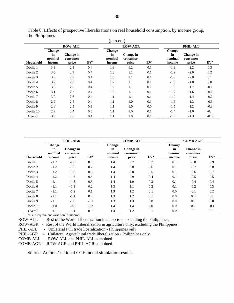
30
Table 8: Effects of prospective liberalizations on real household consumption, by income group, the Philippines
(percent) ROW-ALL ROW-AGR PHIL-ALL
Household
Change in
nominal income
Change in consumer
price EVa
Change in
nominal income
Change in consumer
price EVa
Change in
nominal income
Change in consumer
price EVa Decile 1 3.3 2.9 0.4 1.3 1.2 0.1 -1.9 -2.2 0.3 Decile 2 3.3 2.9 0.4 1.3 1.1 0.1 -1.9 -2.0 0.2 Decile 3 3.3 2.8 0.4 1.3 1.1 0.1 -1.9 -2.0 0.1 Decile 4 3.2 2.8 0.4 1.2 1.1 0.1 -1.8 -1.8 0.0 Decile 5 3.2 2.8 0.4 1.2 1.1 0.1 -1.8 -1.7 -0.1 Decile 6 3.1 2.7 0.4 1.2 1.1 0.1 -1.7 -1.6 -0.2 Decile 7 3.0 2.6 0.4 1.1 1.1 0.1 -1.7 -1.4 -0.2 Decile 8 2.9 2.6 0.4 1.1 1.0 0.1 -1.6 -1.3 -0.3 Decile 9 2.8 2.5 0.3 1.1 1.0 0.0 -1.5 -1.2 -0.3 Decile 10 2.9 2.4 0.5 1.1 1.0 0.1 -1.4 -1.0 -0.4 Overall 3.0 2.6 0.4 1.1 1.0 0.1 -1.6 -1.3 -0.3
PHIL-AGR COMB-ALL COMB-AGR
Household
Change in
nominal income
Change in consumer
price EVa
Change in
nominal income
Change in consumer
price EVa
Change in
nominal income
Change in consumer
price EVa Decile 1 -1.2 -2.0 0.8 1.4 0.7 0.7 0.1 -0.8 0.9 Decile 2 -1.2 -1.8 0.7 1.4 0.8 0.6 0.1 -0.7 0.8 Decile 3 -1.2 -1.8 0.6 1.4 0.8 0.5 0.1 -0.6 0.7 Decile 4 -1.2 -1.6 0.4 1.4 0.9 0.4 0.1 -0.5 0.5 Decile 5 -1.1 -1.5 0.3 1.4 1.0 0.3 0.1 -0.4 0.4 Decile 6 -1.1 -1.3 0.2 1.3 1.1 0.2 0.1 -0.2 0.3 Decile 7 -1.1 -1.2 0.1 1.3 1.2 0.1 0.0 -0.1 0.2 Decile 8 -1.1 -1.1 0.0 1.3 1.2 0.1 0.0 0.0 0.1 Decile 9 -1.1 -1.0 -0.1 1.3 1.3 0.0 0.0 0.0 0.0 Decile 10 -1.0 -0.8 -0.3 1.4 1.4 0.0 0.0 0.2 -0.1 Overall -1.1 -1.1 0.0 1.4 1.2 0.1 0.0 -0.1 0.1
a EV = equivalent variation in income. ROW-ALL - Rest of the World Liberalization in all sectors, excluding the Philippines. ROW-AGR - Rest of the World Liberalization in agriculture only, excluding the Philippines. PHIL-ALL - Unilateral Full trade liberalization - Philippines only. PHIL-AGR - Unilateral Agricultural trade liberalization - Philippines only. COMB-ALL - ROW-ALL and PHIL-ALL combined. COMB-AGR - ROW-AGR and PHIL-AGR combined.
Source: Authors’ national CGE model simulation results.
31
Table 9: Income inequality and poverty effects of prospective liberalizations by location, gender and skills, the Philippines
(percent change relative to 2000 index)
Variablea 2000 Index
ROW-ALL
ROW-AGR
PHIL-ALL
PHIL-AGR
COMB-ALL
COMB-AGR
COMB-ALL
COMB-AGR
Indirect
Tax Replacement Direct Tax
ReplacementAll Philippines Gini 0.51 -0.2 -0.2 0.4 0.3 0.2 0.1 0.1 0.1 P0 33.5 -0.9 -0.6 1.1 0.4 0.1 -0.1 0.0 -0.1 P1 10.3 -1.9 -1.2 1.6 0.4 -0.4 -0.9 -0.4 -0.7 P2 4.3 -2.8 -2.0 2.0 0.4 -0.8 -1.5 -0.9 -1.3 All Urban Gini 0.48 -0.2 -0.2 0.4 0.3 0.2 0.1 0.2 0.1 P0 18.6 -1.6 -0.9 2.0 0.8 0.1 -0.2 0.1 0.0 P1 5.0 -1.9 -1.0 3.2 1.7 0.4 -0.1 0.4 0.1 P2 2.0 -2.0 -1.1 4.7 2.7 0.8 0.0 0.9 0.5
Urban-male-skilled P0 3.2 0.1 0.0 -1.5 -1.4 -0.7 -0.7 -1.2 -1.6 P1 0.7 -1.4 -0.2 -2.0 -3.4 -2.2 -2.6 -3.4 -3.4 P2 0.2 -1.7 -0.4 -2.6 -4.4 -2.7 -3.3 -4.4 -4.3 Urban-male-unskilled P0 23.3 -1.6 -0.9 2.1 0.9 0.1 -0.2 0.1 0.1 P1 6.4 -1.8 -1.0 3.2 1.7 0.5 -0.1 0.5 0.2 P2 2.5 -2.0 -1.1 4.8 2.8 0.8 0.1 1.0 0.5 Urban-female-skilled P0 0.9 0.0 0.0 -2.3 -1.9 -1.0 -1.5 -1.2 -1.4 P1 0.1 -2.5 -0.6 -0.8 -3.1 -2.7 -3.4 -2.8 -3.7 P2 0.0 -4.1 -1.0 -0.2 -4.4 -4.1 -5.2 -4.4 -5.5 Urban-female-unskilled P0 15.2 -2.1 -1.2 1.8 0.6 -0.1 -0.4 0.1 -0.2
P1 3.9 -2.3 -1.1 3.7 2.3 0.5 0.0 0.5 0.1 P2 1.6 -2.4 -1.3 5.1 3.4 1.0 0.1 1.0 0.6 All Rural Gini 0.43 -0.1 -0.1 0.5 0.2 0.2 0.1 0.1 0.1 P0 48.7 -0.9 -0.6 0.6 0.0 -0.1 -0.3 -0.2 -0.3 P1 15.9 -1.4 -0.8 1.6 0.4 -0.1 -0.6 -0.2 -0.5 P2 6.8 -1.7 -0.9 2.7 1.1 0.1 -0.6 0.0 -0.4
Rural-male-skilled P0 12.0 0.0 0.0 -1.4 -2.1 -1.6 -3.1 -1.7 -2.8 P1 3.5 -1.0 -0.2 -1.4 -2.3 -1.8 -2.2 -1.7 -1.9 P2 1.4 -1.2 -0.3 -1.5 -2.7 -2.2 -2.6 -2.0 -2.3 Rural-male-unskilled P0 52.4 -0.9 -0.6 0.6 0.0 -0.1 -0.3 -0.2 -0.3 P1 17.2 -1.3 -0.7 1.6 0.5 -0.1 -0.6 -0.2 -0.5 P2 7.4 -1.6 -0.9 2.7 1.2 0.1 -0.6 0.0 -0.4 Rural-female-skilled P0 14.7 0.0 0.0 -0.7 -2.1 0.0 -0.8 -0.2 -1.0 P1 4.1 -1.0 -0.2 -1.1 -4.4 -1.1 -2.5 -1.2 -2.5 P2 1.4 -1.6 -0.3 -1.6 -6.3 -1.7 -3.7 -1.9 -3.8 Rural-female-unskilled P0 34.9 -1.3 -0.9 0.8 0.2 -0.2 -0.4 -0.2 -0.1
P1 10.8 -1.8 -1.1 2.0 0.6 -0.1 -0.6 -0.1 -0.4 P2 4.4 -2.3 -1.3 3.7 1.6 0.3 -0.4 0.2 -0.1
a Gini = Gini Coefficient; P0=poverty headcount; P1=poverty gap; P2=poverty severity ROW-ALL - Rest of the World Liberalization in all sectors, excluding the Philippines. ROW-AGR - Rest of the World Liberalization in agriculture only, excl. the Philippines. PHIL-ALL - Unilateral Full trade liberalization - Philippines only. PHIL-AGR - Unilateral Agricultural trade liberalization - Philippines only. COMB-ALL - ROW-ALL and PHIL-ALL combined. COMB-AGR - ROW-AGR and PHIL-AGR combined. Source: Authors’ national CGE model simulation results.


