Aircraft electric field measurements: Calibration and ambient field retrieval

JOURNAL OF GEOPHYSICAL RESEARCH, VOL. 99, NO. Dll, PAGES 22,781-22,792, NOVEMBER 20, 1994

Aircraft electric field measurements: Calibration and ambient

field retrieval

William J. Koshak 1 Earth Systems Science Division, Marshall Space Flight Center, Huntsville, Alabama

Jeff Bailey, 2,3 Hugh J. Christian, 2 and Douglas M. Mach 2 Johnson Research Institute, University of Alabama, Huntsville, Alabama

Abstract. An aircraft locally distorts the ambient thundercloud electric field. In order to determine the field in the absence of the aircraft, an aircraft calibration is required. In this work a matrix inversion method is introduced for calibrating an aircraft equipped with four or more electric field sensors and a high-voltage corona point that is capable of charging the aircraft. An analytic, closed form solution for the estimate of a (3 x 3) aircraft calibration matrix is derived, and an absolute calibration experiment is used to improve the rela- tive magnitudes of the elements of this matrix. To demonstrate the calibration procedure, we analyze actual calibration data derived from a Lear jet 28/29 that was equipped with five shutter-type field mill sensors (each with sensitivities of better than 1 V/m) located on the top, bottom, port, starboard, and aft positions. As a test of the calibration method, we analyze computer-simulated calibration data (derived from known aircraft and ambient fields) and explicitly determine the errors involved in deriving the variety of calibration matrices. We extend our formalism to arrive at an analytic solution for the ambient field, and again carry all errors explicitly.

1. Introduction

In situ aircraft observations of the cloud electric field, dat-

ing as early as Gunn et al. [1946], have played a significant role in the scientific study of cloud electrification, lightning phenomenology, and aircraft lightning protection. The type of aircraft, the number and type of electric field sensors, the data acquisition system, and the theory for inferring the ambient field have varied widely [Winn, 1993; Kositsky et al., 1991; Jones, 1990; Blakeslee et al., 1989; Bailey and Anderson, 1987; Laroche et al., 1985; Christian et al. 1983].

in general, aircraft field sensors do not directly detect the ambient thundercloud electric field, E. Instead, the sensors detect the aircraft-enhanced ambient field, the aircraft self

charge, Q, and a variety of other effects due to the presence of the aircraft including: engine exhaust charges, corona discharge, polarization charging, and field perturbations due to aircraft-caused turbulence. If an aircraft builds charge due to particle impaction, the hot engine exhaust plume can subse- quently discharge the aircraft and redistribute atmospheric charge thereby changing the ambient field. Similar statements can be made about corona discharge where pointed objects on

I Marshall Space Flight Center, NASA, Huntsville, Alabama. 2johnson Research Institute, University of Alabama, Huntsville,

Alabama.

3Now at Hughes STX Corporation, Huntsville, Alabama.

Copyright 1994 by the American Geophysical Union.

Paper number 94JD01682. 0148-0227/94/94JD-01682505.00

the aircraft frame serve as another means for removing charge from the aircraft and redistributing it into the atmosphere. Since charges move freely along the conducting surface of an aircraft, the aircraft can become polarized so that even without having accumulated net charge from particle impaction, the polarization charge may be removed via the exhaust plume or through corona discharge. Again, the charge distribution in the atmosphere is changed resulting in a change in the ambient field. The reader is referred to Jones [ 1990] for further details on aircraft charging. Aircraft-induced turbulence has the effect of reorganizing charges in the atmosphere since the aircraft disturbs the natural flow field (and charged particles carried by this flow field) in the atmosphere. Overall, in order to determine the true ambient field from aircraft measure-

ments, it is necessary to remove all perturbations of the natural ambient field due to the presence of the aircraft.

In this paper, we introduce a matrix inversion method for calibrating an aircraft (section 2), and we discuss fundamental limitations in the accuracy of any calibration method (section 3). To the best of our knowledge, our formalism is the only one that introduces a closed form analytic relation between estimated and true aircraft calibration coefficients with all

errors explicitly cited. All other effects due to the presence of the aircraft (e.g., net aircraft charge, polarization charge, corona discharge, engine exhaust charge, and aircraft-induced turbulence) are treated as additional (or virtual) measurement error so that the linear theory we apply maintains generality. To demonstrate the calibration method, it is applied to data derived from a low self-charging Lear jet 28/29 equipped with five shutter type field mills (section 4). In section 5, we per- form mathematical tests of the calibration method. This is

done by selecting several arbitrary aircraft with known enhancement characteristics, simulating realistic errors, and

22,781

22,782 KOSHAK ET AL.: AIRCRAFT ELECTRIC FIELD SENSING

applying the calibration procedure to derive calibration solutions. The solutions are compared directly to the known aircraft enhancement characteristics to validate our procedure and to quantify the typical solution errors. Finally, we describe the errors in the retrieval of the ambient field, E (section 6) and summarize our results (section 7).

2. Method

We begin by considering i = 1 ..... rl, where rl > 4, field sensors arbitrarily located on an aircraft that is equipped with a high-voltage (> l0 kV) corona point. Each sensor measurement, a i (in volts/meter), is proportional to the aircraft enhanced ambient field, the aircraft enhanced net charge, and

all other influences that we shall regard as errors, e i. These errors include, but are not limited to, sensor electronics measurement error and field fluctuations due to engine exhaust charges, corona discharge, polarization charges, and aircraft- caused turbulence (see section 1). Collecting the rl measure-

ments into one vector, ap = col(a • ..... an)p, for the p th aircraft orientation, we have

a• = Mv p + • . (1)

Here we have identified for shorthand notation a source vec-

tor, vp--col(Ep, Qp), with E denoting the ambient electric field and Q the net aircraft charge. The enhancement of this source is given by the enhancement matrix, M. An element,

Mij, j -- x, y, z, q, of the enhancement matrix represents the enhancement of the j th source component at the i th sensor

location, e.g., M2y would represent the enhancement of the y component of the ambient field at aircraft sensor location 2. Finally, the error vector is defined as ep--col (e I ..... erl)p.

One approach for calibrating an aircraft involves using

measurements, ap, and estimates of the source, Vp, for several aircraft orientations in order to infer the aircraft enhancement

matrix M. (Note that once this matrix is known, a suitable inversion of (1) will provide the desired source vector, vp, along the aircraft track given measurements, ap.) Although the task of estimating net aircraft charge is difficult and depends on the particular aircraft in question, it is generally possible to make reasonable estimates of the ambient field. This can be

done by performing a variety of aircraft maneuvers in fair weather where the direction of E is vertical and its magnitude is known to within reasonable bounds.

Since in this paper we are ultimately interested in determining only the ambient field, it will not be necessary to deal with estimations of aircraft charge or in determining the explicit elements of M. Instead, our approach will be to mathematically filter aircraft charge [see Winn 1993] from (1), so that only estimates of the ambient field will be required to calibrate the aircraft.

During straight and level flight in fair weather we have E x -• 0 and E y -• 0, and the ith component of (1) reduces to (suppressing the p subscript for brevity) ai(t ) -- MizEz(t ) + MiqQ(t) + el(t). If at a later time the aircraft is charged by placing a high voltage on the aircraft corona point, we have ai(t+At ) --MizEz(t+At ) + MiqQ(t+At ) + ei(t+At ). Since the variation in the fair weather field along the flight path of the aircraft is negligible compared to corona point-induced changes in aircraft self-charge then Aa i -- [ai(t+At)-ai(t)] -• Miq [Q(t+At)-Q(t)]. Hence any ratio of "Q-coefficients" can be estimated, e.g., Mlq/M2q is approximately the ratio of A a I

to Aa 2' If we write the measurement ratio as ,k•v-- Aa u/Aav and the Q coefficient ratio as )•uv -- M uq / Mvq, then the error in estimating the Q coefficient ratio is

!luMvq - !lvMuq Mvq (Mvq +/.t v )

lai = Mizl aEz )+( aei ) (2)

where i = u or v. Since AQ >> AE z and AQ >> Ae i, It u and It v are both close to zero so that •5 uv -• 0.

Using the ratios, 3.•v, linear combinations of the field sensor data can be formed so as to approximately eliminate Q. In effect, we replace the Q-sensitive measurements, ai, with the relatively Q-insensitive values, .Euv = .E k, given by

.Ek= •.kav-au, k= 1,2,3,-..,m

(//-2)!2!

(3)

For brevity, we have compressed the (u,v) indices into one index k. Note that when two aircraft measurements are com-

bined in this way there are a total of m distinct combined measurements, that is, m is a combination of q measurements

taken two at a time. Removing the measurements a u and a v in (3) with the help of (1), we obtain for the pth aircraft orientation the (m x 3) system

.•p = KEp +•p, (4)

where the calibration matrix K has elements

K•j =J.* (5) •M•j - Muj,

and k -- 1,---,m;j = x, y, z. Note in this case that we have limited the range on the j index. The (attenuated) term proportional to Q has been assigned to the column vector of

errors, •p, having components of the form

ek =SkMvqQ+J. kev-eu, (6)

where the p subscript was suppressed in (6) for brevity. Note from (5) that the calibration matrix, as we have

defined it, depends itself on the experimental errors in the high-voltage corona point experiment, i.e., Kkj depends on /l k. This implies that if two (distinct) corona point experiments were conducted with two identically shaped aircraft, the resulting K matrices would, in general, be different (however, this difference should be small if the corona point experiment is reproducible). Nonetheless, the only important requirement is that the ambient field is retrievable as is allowed by inversion of (4).

Although there are several equations available to retrieve the three components of E in (4), i.e., m > 3 for rl > 3, not all of the m equations in (4) are independent. For instance, with only three electric field sensors (rl -- 3) we obtain three derived measurements: {œ 12,-/223, ./2 13 )' It is trival to show that in this case the resulting K matrix is singular. With four

KOSHAK ET AL.: AIRCRAFT ELECTRIC FIELD SENSING 22,783

sensors, and derived measurements: {d•12 , d•23, d•.34 }, K is an invertible (3 x 3) matrix. For these reasons, we require four or more sensors (r I > 4) to retrieve E. (Note' if external con- straints are employed [see Tworney, 1977, chapter 6], fewer than four aircraft measurements could be used to infer E, but this approach is not considered here.)

To obtain the best estimate of Ep, we consider aircraft calibration maneuvers during fair weather field conditions: E x, = O, Ey, = 0, and •-- E z, < 0, where the primed coordinate system indicates the Earth frame. Under these conditions, the

components of Ep can be written as

f sintip Ep=•p sinapCOSflp -- •pfp, (7)

LCOS%COS/.

where Ctp is roll angle, [•p is pitch angle, fp(a,p, [•p) is a unit vector describing the aircraft orientation, and the pitch matrix transformation was performed first. Our convention is that of a right-handed coordinate system where the +x axis points into the direction of flight, the +y axis along the portside wing, and the +z axis defines the aircraft zenith. Rotation of y into z defines positive roll angles, and rotation of x into z defines positive pitches. Due to the noncommutivity of orthogonal roll and pitch matrix transformations, the order of rolling and pitching is, in general, important. However, when (lp and/or [3p is small (as will be the case in all analyses below), the order of rolling and pitching can be neglected, and (7) is valid. We have assumed that any rotations about the aircraft zenith (following rolls and/or pitches) are negligible; pitch and roll angle accuracy of 0.2 ø is assumed. Note that a subscript "p" has been attached to the variable • since the fair weather field varies with altitude, z', and different aircraft orientations may occur at different altitudes (e.g., when the aircraft nose pitches downward, z' decreases). An empirical formula for •(z') due to Gish [1944] is

•'(z')=-[81.Se -4'52z' +38.6e-ø'375z' + 10.27e-O'121z' ] , (8) where z' is in kilometers and •(z') is measured in volts per meter.

Using (7), we may rewrite (4) as

œ, = sepKf , + •,. (9)

In this equation it is important to note that within the linear

theory, •p and K are understood to be the true fair weather field and aircraft calibration matrix, respectively. Next, our ¾th estimate of K is the matrix K T defined by the equation

œ p = •prKrfp, (10)

where •p•, is the Tth estimation of •p. Equation (10) assumes we know the true aircraft orientation fp, that is, we neglect roll and pitch angle measurement errors.

Following Twomey [1977; chapter 9], we can solve for K? t

directly by post-multiplying (10) with f p, summing over all n aircraft orientations, and inverting. We obtain

•' • , (11) p=l

where the (symmetric) covariance matrix is given by

1• fpf• C---- n

p=l

(12)

and the t superscript denotes transposition. In practice, it is not difficult to implement the matrix solution in (11) on a computer. However, some care must be taken to assure that a

variety of aircraft orientations are chosen (that is, if only straight and level orientations were chosen, C would be singular and hence noninvertible).

At this point it is instructive to relate the computer solution

given in (11) to the true calibration matrix, K. Eliminating œp with (9) gives

Ky=K[•p •'P fpf•]C-' +[nl-- p• I •pf•]C-I •py • . (13)

The first term on the right-hand side is an "information term" since it is proportional to K, whereas the second term is an

"error term" proportional to ep. From (13), the best estimate of K is obtained when •p•, is a good estimate of •p and the errors, fp, are small. If • = •p, and •p = 0, then K v is identically equal to K. Thus whenever •p is negligible, the primary task in getting a good estimate of K is to somehow obtain a good estimate of the fair weather field. In most cases, we can

assume that the error •p is within 10%. If, for example, we substitute •p •- _+0.1 •Kfp into (13), we find that the information term can also be retrieved to within 10% (note that this does not mean we would retrieve the elements of K to

within 10% because the information term itself is subject to large errors if the estimate •PT is poor).

Assuming then that the error term in (13) is negligible, the question arises: is there a way to choose a good estimate •PT •-- •p without having directly measured •p? To answer this question, we can begin by assuming a first guess • ---1 and recognizing that the true fair weather field can always be bro- ken up into a mean (•av) and perturbation (Se'p) part, that is, •p--•av + •"p = •av' Here we have assumed that the mean field is large compared to the perturbation part (the maximum perturbation is attributable to pitches and, in the case of the Lear jet, was less than about 20% of •av )' With these approx- imations, (13) simplifies to (for ¾ = 1)

Ki •- -•'av K. (14)

Now, results from an absolute calibration experiment can be used to help determine •av' In an absolute calibration, straight and level aircraft maneuvers in fair weather are flown tens of feet above a ground-based field sensor. Such an experiment allows one to determine the last column of K directly, that is, using (9) we can, for instance, obtain Kzz from

.12Z -- gKzz q-E z (15)

Kzz --

where the ground-based measurement of the fair weather field,

•g, approximates the value of the fair weather field at the aircraft, •' that is, • = •g + Ag. Using (14) and (15) gives

22,784 KOSHAK ET AL.' AIRCRAFT ELECTRIC FIELD SENSING

•g 1 -•av = K:g• = Kzz I = (16) Kzz œz Sl

With the help of (4), (14), and (16), a new estimate of the fair weather field can now be obtained as

>-, = (17) For such a test to be valid, • must be sufficiently small (that is, corona discharge, polarization charging, exhaust charging, aircraft-induced turbulence, and sensor electronics measurement error must all be small) and K must not be ill- conditioned (that is, the field sensors should be orthogonally placed to assure measurement independence). If K is ill-

conditioned, errors of the type K-I• will be quite large, thereby invalidating (17) (see Twomey [1977] for more detail on error magnification and the inversion of ill-conditioned matrices).

To summarize the calibration procedure, one performs n calibration maneuvers in fair weather and stores the data set

of measurements, .E•,, and aircraft orientations, f•,. With an initial estimate, •,l ---1, (11) provides the matrix K •. A new fair weather field estimate, •2, is computed using (17), and (11) is used to compute K 2. The final calibration matrix solution, K*, is obtained as

K* s2K 2 œz = - K 2 =K+B, (18) •gKzz2

where B is an error matrix to be described below.

Finally, we note that if the aircraft net charge is small compared to the ambient fair weather field magnitude, the matrix solution described above may be applied directly to the system in (1). In this case, the last column of M is removed and the solution given in the appendix applies; that is, all field enhancement coefficients are explicitly obtained even if the aircraft is not equipped with a high-voltage corona point.

3. Fundamental Limitations in Retrieval Accuracy

As with all inversion problems, there is an upper limit to the degree of detail the measurements can provide about the unknown distribution (matrix elements in this case) (see Twomey [1977] and Koshak [1991] on information content eigenanalyses in linear systems). Using (13) with the estimate, •,2, and identifying the estimation error, A•,2 -- •, - •2, the error matrix, B, is given by

1 B=s2 • '•2 (A•o2Kf•ø + t•,)f[]C -t +(s2-1)K

•m:5; + E:[ s 2 = (•_ Ag)Kzz2(K,A p, •p)

(19)

Here we have indicated the explicit form of the correction factor s 2 in terms of the absolute calibration measurement œz, the absolute calibration errors A g and e z inherent in (15), and the errors A•, and ep in K zz2 as prescribed by (13). The error matrix conveniently summarizes all errors in the retrieved calibration

matrix in the form of a matrix function B -- B (e•,, A•, 2, A g, œ z). If each argument of this matrix function is zero, then s 2 -- 1, B is the zero matrix, and our solution K* -- K. Note that the elements of B are large when the elements of K are large.

In addition, the percentage error in the retrieval of the (j, k) element of K is

I. (20)

Since it is possible for elements of B to be large even when corresponding elements of K are small, percentage error in the retrieval of small elements of K can be expected to be large.

4. Application of the Calibration Method

To demonstrate the calibration method, we analyze realistic calibration data derived from Lear jet 28/29 fair weather field maneuvers at the NASA Kennedy Space Center, Florida. Five field mills, each with sensitivities of better than 1 V/m, were mounted on the top and bottom centerline of the Lear jet, and on the port, starboard, and aft (tail) locations as shown in Figure 1. Additional details of the aircraft, mill sensors, and data acquisition system are given in J.C. Bailey et al. (unpublished report, 1994).

For this application we have used just three of all possible Q-insensitive measurements, œk, that are obtainable from this aircraft system, that is, we work with the simple (3 x 3) determined system rather than an overdetermined system (see section 2). The second and third components of .E were formed by combining the port and starboard measurements and the top and bottom measurements, respectively, as given in (3). The first component of .12 was obtained by combining the port and

A

Stinger Probe

Electrical Field Mill Sensors

Figure 1. The Lear jet 28/29 aircraft and the location of the electric field mill sensors. A fifth mill is located on the starboard side.


(a) Roll Angle

30 -'

0 300 600 900 1200 1500 1800 P

9O

45

-45

-90

(b) Pitch Angle I ß ß I ß = I ß ß I ß ß I " ß I ß ß

'1 , , I , , I , , I , , I , I , , I' 0 300 600 900 1200 '1500 1800

P

Altitude 2

1.6

1.2

0.8 0.4

0

0 300 600 900 1200 1500 1800

P

Figure 2. (a) Roll, (b) pitch, and (c) altitude data for each pth Lear jet calibration maneuver in fair weather. Data were taken on July 10, 1990, from 1818:09 to 1821:58 GMT and from 1827:01 to 1831'51 GMT.

aft measurements (we have also added to this a similar combination of the starboard and aft measurements). In this way, the first, second, and third components of œ depend largely on E x, Ey, and E z, respectively.

The raw data set consisted of field mill measurements (ap), roll and pitch angles ((xp and I• ), and aircraft altitudes for a total of n -- 1750 aircraft orientations. These data were derived

from flight maneuvers on July 10, 1990, from 1818:09 GMT to 1821:58 GMT and from 1827:01 GMT to 1831:51 GMT; the roll/pitch and altitude data are shown in Figure 2. The specific aircraft orientations selected from these manuevers were

primarily centered on rolls of +45 ø, pitches of +15 ø, and level flight. Only those rolls of +45øthat were associated with pitches within +5 ø of zero were used, and only those pitches of :t:15 ø that were associated with rolls within +5 ø of zero were used. For these data, the calibration method gives the solution

F61.14 -0.01 15.571 K* =l-O.4 3.05 0.07l. (21)

L-1.22-0.35 7.20_]

To obtain (21), the values of s• and s 2 were computed using results from an absolute calibration experiment (see section 2). The experiment consisted of seven low-level overflights (altitudes of 20, 25, 25, 50, 50, 100, and 100 feet) above a

ground-based field mill at the Cape Canaveral Air Force Base (CCAFS) Skid Strip on March 8, 1992. From (15) we obtained a value of K= = 7.2 _+ 0.32.

Figure 3 gives the retrieved estimate, •p2 that was used to generate the solution given in (21). Comparing this plot with the altitude plot given in Figure 2c, we see that there is gen-

-20

-40

-60

-80

-lOO

• I I I I i I i I I i i I I

: ß : ; ß •

kl I I I I I I I I I I I I I I I 0 300 600 900

P

I I

1200 1500 1800

Figure 3. Derived fair weather field estimate that is used to compute the final calibration matrix for the Lear jet.


erally favorable correspondence, that is, as the aircraft climbs, the fair weather field magnitude decreases. There are some

oscillations in the plot of •e2 (e.g., the positive spike near p -- 900) that are attributable to measurement en'ors, •t, (see section 5 below for more details on retrieval errors).

5. A Test of the Calibration Method

In order to test the calibration method described in section

2 above, we can select an arbitrary aircraft with known enhancement coefficients and known corona point experimental results (that is, we can pick a known K matrix), and "fly" this hypothetical aircraft through a known fair weather field.

We can then select the aircraft orientations, re, and the errors, •, and compute each pth measurement, •e, using (9). This computer-generated calibration data set, {•p, f p}'p = I ..... n , along with an assumed absolute calibration result for the magnitude of Kzz (with possible assumed absolute calibration

errors), are all that is needed to compute K*. The solution matrix, K*, and •2 can then be directly compared with the corresponding known values. To the best of our knowledge, direct simulation tests of this nature have never been applied to any aircraft calibration technique in the past, yet these tests mathematically clarify the overall performance of a particular calibration method.

To make the simulation as realistic as possible, we use actual aircraft orientation and altitude data (obtained from the

Lear jet) as shown in Figure 2. Assuming these Lear jet maneuvers were performed in a fair weather field profile given by (8), we obtain a known fair weather field, •, as shown in Figure 4a. We choose for our known K matrix the solution given in (21) for the Lear jet.

Aside from some enhanced peaks, the iterative calibration method retrieves the known fair weather field quite well when there are no errors except computer truncation (Figure 4b), is offset by a constant factor when there is a large positive abso-

-20

-40

-8O

-lOO

-20

...-4o

-8o

-1 oo

(a) Fair Weather Field (GISH, 1944) I I I I i i I i I I I i I i i I i i I

I I I I I I I I I I I I I i • I i i I 0 300 600 900 1200 1500 1800

- 0

• -40

•0

-100

I i

(b) Retrieval (meas err = 0%, abs cal err = 0%)

I I I I I I I I I I I I I I I I I

&•rms = 1.1 V/m - --

--

_ --

-

-

--.

I I I I I I I I I I I i I • • I

0 300 600 900 1200 1500

p

i i I

1800

(c) Retrieval (meas err = 0%, abs cal err = 50%)

I I I I I I I I I I I ! I I I I I I I

A •rms = 13.2 Vim

(d) Retrieval (meas err = 10%, abs cal err = 0%)

A •rms = 2.3 Vim

I i i I , I I [ I I I [ I I I I I I I 0 300 600 900 1200 1500 1800 0 300 600 900 1200 1500 1800

p p

Figure 4. (a) Known input fair weather field, and (b-d) retrieved fair weather fields for various errors. Note the dc offset in the retrieved field that had an absolute calibration error and the high-frequency noise in the retrieved field having a nonzero and random error, •p.


lute calibration error of 50% (Figure 4c), and is a reasonable, but noisy, retrieval in the presence of a 10% random error, •p (Figure 4d). An assumed error of 10% should be quite reasonable as the calibration maneuvers are performed in fair weather where the effects of corona discharge, polarization charging, and charged particle impaction are negligible. Note that the rms retrieval error in Figure 4d was only 2.3 V/m. Using the result in Figure 4d for our estimate of •p2 gives the solution matrix

[57.64 -0.22 15.291 K* =/-0.16 3.02 0.06 . [-2.46 0.42 7.20

(22)

Comparing (22) with (21), we see that the retrieval error is within 10% for the large matrix elements and that the per-

centage error, P, is much larger for the smallest elements in accordance with the discussion in section 3. The absolute error

in the retrieval of the smallest matrix elements is less than the

absolute retrieval error in the large elements. To build more confidence in the calibration method, we

next create 500 different known K matrices (based on ran-

domly adding a 50% fluctuation to each element of (21), e.g., Kxx -- K•a. + 0.5*r*K•., where r is a random number between -1 and 1) and retrieve matrix solutions, K*, for each. The results for a random 10% error in both • and the absolute calibration result for Kzz are given in Figure 5. Here we have plotted the matrix retrieval error, Bjk, versus the associated known matrix element, Kjk. Again, the small elements of K are retrieved poorly percentage wise, but they are also associated with small errors, IB/kl. From the standpoint of accurately inferring E (see section 6 below), the absolute errors, lB/k I, are more

14

x

-14

• I I I I-

ß' - 'a.• ß . '. ' .re, •' ß , . . .-; . I.., ß

:', ½.:...'% .. ß i'..},, '.' .... :':.'• , .'.'. ß ß ..: ..:•/ß .,: ......'.'_.,•}. '.-. •.., •'- .... %-. ß ' '. - ße . .'- %, .' ß . .. ', ß . ß :.. : .'.. ß ß .

ß _

'1 I I I I

30.5 45.75 61 76.25 91.5

Kxx

0.55

.275

ß 0

ß '"" I'1 i"' 'l' " ' : ''' ' ':' '::'i:, t' "-" ';' !' ..',:,.t', .:,' .' ,4' .'I, '-! ' .275 '"'-i.",;."l.':'";.':t.-",','.:':l',: :; .! ,J:l:..'iS.,." ' •.,•-•

:....,......:-.,..... :.:7!' ,,,' :";.'.

0.55 I I I '"' I' ; I1 -9.9E-3 -8.25E-3 -6,6E-3 -4.95E-3 -3.3E-3

Kxy

2.5

1.25

o

-1.25

-2.5

0.1

0.05

• 0

-0.05

-0.1

ß .

ß .j.. ß .: • .- ..? . .' ß '"•' : •"• -:' •"t' 'ø•"'""'•

?. •..,'.".•,•. ..-.,..,., .,•';.'..::,:,- :. ß ...,e '•. t. ' 1•' ' '6"6 :*g e 'e•' '., '-' .'• ' 'it'.; ' Z t,.% , •'. . , ß ß ,& . ß .# ß . .,,... .1 . ß ß .I.;•... .½ ,,,,_.' o .... .....'.:. ß ß., ß g' . : : .... ß ...... ß . .. • ..• ß o •. ' ß ß ,.: J . .' . -

ß . ß .

ß

.

'1111 III1' '' ,,, I,,, ,,, I,,,, ,,I

-0.21 -0.1 75 -0.14 -0.105 -0.07

Kyx

0.72

0.36

0.36

0.72

-I I I I I--

-I I I I I'

1.5 2.25 3 3.75 4.5

Kyy

0.02

0.01

-O.01

.0.02

-I I I I I-

..'

.... ß., .. .:- ß :: -•1

• '.. ' .. ,,.-... %. -- •' ' •'•,.. q..•;•..:,:'•.';.,';':z' , r% q.,. '%•1 '-.'S. '..,..: .'. ø ß "-•J - ß '.A'.'"._ • ß ' .? 3. ß •. ß ' , . ß ß .. ß .: %0, ,,,. '.'el'= ß ß ,q•.•. ,& %•

-•. . ß: .....' ,.'.',.:. •:' •:" .. %'. ß . . ':.:.

ß

'1 I I

0.035 0.0525 0.07

j-

0.0875 0.105

Kyz

2.4

1.2

x 0 N

-1.2

-2.4

-I,, I,, I,, I, • I1 0.24.-I I I I I 1.3 0.12 0.6•

.,.•- ,., ..- . -..j. ;,:.:.•j .........: . .,.... .... . ,• o ..,............... .. ß , ,• c

ß ' ' t '% .' 8 ' ' ..'..: .... ,'. ,.. :,.:'- .: .-' .. :-7 ;, .:,•¾..::,:•';.t•.. ,. ;,..,¾.':..'•:, .'....,: ::' ;1 j,-:. :,:.'-.- '.. = '... ß t-'.',',' .- !' :'::,,:':.'!,'•;'•'.i':.. '. _q-•.';'•'..:';.' :-'-,'•.•.•'J :. ;, ,.. ' ,',.'.:'! ,,,-..., ,'•_1'.' ß '?,.'... :• -I : ':-;.•.;-'.:."'•.• -.;..o'.;.'".•'C ..' ".-"7.'...•! -0.12 I- '.'.'j.,' ..•-,.'•.'-" :' ':,.•:-: :.' •..'• ,'r';.?l --0.65 " '"'"" ''"'""" ' .... " "-I I-- ß .'.:..-.%,'?:."'• ".•" .: ' -..--I '''"'"" "' ' ' ":''':" '' [:"':"': "" ''"" ?' '"'':' ' 't -1.3 I i I I I I I I I I ,' , I'-] -0.24 I-I "' ' I' ' ;' I * I' ' I-!

-' .8 -1.5 -1.2 -0.9 -0.6 -0.525 -0.4375 -0.35 -0.2625 -0.175

Kzx Kzy

I ] ' I ' ' I ' t I • I I.• ß I e•_ ß •'% o * ' ' '

. :';' ß ,. • '•..•'. %' •: •j .- ß I0 ' ß •' •. .. * '. ' L • .... .•/..2 -:• t' . .' -

•.-[•-"/.•'-", ...•- - ..,... ['•r '..-? i.•'•i•:<':;%, '. • '•'-•." - rhv,.•r •'. .,.:'.[ '- _.:. -' .- •..r.•;•;'. y %. . ,,3:' :'? •.-

• .... ..•. : ß .... ;%..• . . : ß . '•.* ß .-..... • .' _ ß . ..%' %%..% '.

J I I I , , I , , I , , 3.6 5.4 7.2 9 10.8

Kzz

Figure 5. Calibration matrix element retrieval errors for 500 known K matrices that were produced by randomly varying each element of the solution given in equation (21) of the text by 50%.


12I I ' ' • ' ' • ' ' • ' ' • 1.1 6 0.55

ee e,e ß ße e,, • 'm ß I ß ß ee I' 'ee ß ß ....._,•.: . :.....•:...:.. •.:,.•j.. 0 ß : ..•. ...'. : .: ß ' • c

ß: .:. -.:, •, .-'?...._'../....•'..,.• •, .'..."* • ß • '.._ .. •.•""-- .,•.•,..• . ' ß -0.55

s '•o.-•... • '.,'.'..•'• .... .?'... :.:.

-12 '1 "• ** I • , I • • I , , I -1.1 55 58 61 64 67

Kxx

2.7 I I ' ' I ' ' I ' ' I ' ' I . . ß .. .... . '. 1.35•- . , .¾... .... ...... •..'• .... •;, ;,, ....; : :.,.,,'..'.; .'

,e,. ßt. .e, •',, ße. ß ' ' ß o • .'...;,';....., . -:;..j.', n• 0 I- . '• ß •, . I .ß' ß "., '" ß ß • ' ,, .' / ' %;--.'•, ...:;•',;".. '...:.. ':."• / : ,. '," ' ' ß '"'. -•' '-- ' "'. "' ' ' /' ,A'" ß ', '_. 1• .""•' _ .'. • ß •'. / ,'•.s' i ;.. ß" ß '-.'. •.

-1.35 • ß . •,-' ..-.'. '" ".."• '.:

• ß ee eß e I, e / ß ß e. ß ß . .. ø.'• -. ß -

-2.7 I I I I , , I , , I , ,' I -7 -3.5 0 3.5 7 10 13 16 19 22

Kxy Kxz

2.4 1.2[• ' ' • ' ' • ' ' ' ' ' '- 1.2 0..6•- ' " ' • , ...' ß ..• ,;...,i ,

r;...• :: ;" , •':";•;- ß • ß . eee e•e• • e• o ß I ß ß x ''.• .' M''. . '.-- •,.. ' •..'. ,'.v :,'

[. ß .-....;,.:.?.,...•.:. '.:. ø o '.•.' .... ' -1.2 -0.6 - ' '' "' "ß ".' ©e e le

-2.4 -1.2 -I I I I , , I , , I , , ! ' -7 -3.5 0 3.5 7 -3 0 3 6 9

Kyx Kyy

0.6

0.3

-0.3

-0.6 '11111111111111111111111111111'

-7 -3.5 0 3.5 7

Kyz

ß ß ß

ß .) . . 4 :•. ;• '" ß 1.2 0.4 ". -.. •.' 0.65 . •. o;..,- '•

.:.... .... .,. •'-- :. ß .•. ,-...'... . o•r:•.:-.*: ,. '"- ' :' •/'..,..A . '. *:. , ' . a-', '•' ;'• "- ":•

F' -. "' ' ' ' ' - ß ''. ß .' ß - '"''* ''.- ' •." ' N .A.-'."." •:ß..;'•:"t"•' '':'•';". ß '"' "' ' ' ' • • >' o., ,-' .:-• .... • 0 • 0 .... ,.,. ::;•-• ...,..... ;. -] • 0 . .•_•. ',.:'.:½,•'•"i'g'•',-.' '•..- •..-..,-:ø:•:r;.•.•.-•:• ß :: :. •',•::;':."•'•, :•..." ,".•27• •.' • -'.'.-,, :' ,•.•!••::" ß '•'•",•:.'. ,..•-'r' .' ..'ld,. ß .', %rS $ .,e . ' ß ß' . .. . .. •. •_ ,,..,.,•..•., :..•'•,.. '...;•-'1 ø '-:'"';"'"ø"'"'-":•'";': ' :':"' •'•" ß ' '"" -' -1.2• ß ß •'/•" ':'•'o)' ',•'..'•"•- ½o ,.• -0.4 -0.65 [ ' .',. • .•, ß "-h ß •.',•." '. ! ""' '" .... ' :•"; [ ": ,. -2.41-1 I ' , I • • I • • I , , I-I -0.8 ,, ;,,, ,,,,,,,,, ,, ,, ,,, ,, ,,, -1.3 I I I " I -7 -4 -1 2 5 -7 -3.5 0 3.5 7 0 3.75 7.5 11.25 15

Kzx Kzy Kzz

Figure 6. Calibration matrix element retrieval errors for 500 known K matrices that were produced by randomly varying each element of the solution given in equation (21) of the text by the uncertainty + 6.1 (that is, 10% of Kzz ).

important to consider. The percentage error in retrievals of the larger elements of K are all well within 20%. Note that the large elements Kx•; K•z ' Kyy, and Kzz all display a cone type scatterplot shape indicating that IBjkl increases with IKjkl as predicted in section 3. Note that the somewhat borderline element K a. is fairly small but not negligible, yet it still has fairly large percentage error. Once the. magnitude of an element approaches about 3, like Kyy, the percentage error in the retrieval is suitably small. Finally, note that the B zz versus Kzz plot is a simple cone-shaped pattern and is symmetric about the zero line with a percentage error retrieval of +10%. This is to be expected, since we repeatedly correct the K zz element to within the 10% random absolute calibration error

implemented in this simulation. Since many of the elements of the known K matrices

described in the above paragraph are small and remain small

when a 50% fluctuation is added, another simulation test was

performed that adds to each element of (21) a fluctuation between-6.1 and +6.1. This gives at least a 10% fluctuation

about the Kxx element of (21) and substantially more fluctuation about the smaller elements of (21) than given in our pre- vious test. Figure 6 shows that the results are again favorable and similar to those provided in Figure 5. Figures 5 and 6 represent the typical retrieval errors associated with the Lear jet solution given in (21).

As a final and more general test (that is, for more arbitrary aircraft), 500 known K matrices whose elements ranged randomly between 0 and 100 were analyzed. The results are provided in Figure 7. Since all elements of K can now become large, the conelike pattern is prevalent in all error plots (again, the B zz versus Kzz plot is symmetric about the zero line). The calibration method does quite well. The percentage


x 0

-32

_1 .... I .... I .... I .... I ß

ß

ß 42

ß ,

........ •"':"" I •' ' ',•" ß '.'- ß I:-! 0

-42

I I I I I I ß I I I ] I I i I I I I I 114 -84 0 25 50 75 100

II II II,.,, , I ,, ,, I,, ,i I 0 25 50 75 100

Kxx Kxy Kxz

90

45

•, o

-45

-90

60 40

-60 I --40 '1 , , ,, I , , , , I ,, • , I , , , ,I -120 -80 0 25 50 75 1 O0 0 25 50 75 1 O0

IIIiiiiiiiiiiiiiiiii1_

Kyx Kyy Kyz

x 0

32i[ .... ] .... i.,.,. [ • ' ' ' i_ 130 ß

16 . 65

I . . ß ß ß ß ß ' ß ß ß d. eøee •

I: ß :...."'9• ;•_'.. •_-_..-.,•.•H. ri.,: .,.•. -. l ' "" "%'•'"'-'•' ".-' 4. 'b .• -l, •

-16 [.. '- ' -":•%'-C'-_'. -65

f ' -32 - 130 I I IIII i,, •1 •, I I [ I I I I [ 0 25 50 75 100

I .... I .... I''''1''','1 ß

ß

ß

I I I I I I, , I I I I I I tl i ,,, I o 25 50 75 1 oo

;, % '.% -.. ß .':' %' t -'; •' d ."ø'- • ..... ' .... ß ' -,,.•-'5' ;" ' '" ' "" .•..N, ": ....-

o[_•..,'•.•-.,..:..."'. '-.. :t 4.'. .- .' I- "•2. 3'''e ,P ..'-:#. ß ß e. . '•': .,,• ß .. • . • -. "% .., '. .. ,.

L ..- •;,It . q"l:.'. .; : . '5 F ' TM ;' •'"'x. "/"' '

i ,. ':.:• '•'ff.'..: o i i i i i i , • • , i , • , , i , ,', i';[ o 25 50 75 1 oo

Kzx Kzy Kzz

Figure 7. Calibration matrix element retrieval errors for 500 known K matrices that were produced by randomly varying each element between zero and 100. Large errors are only associated with small (and unrealistic) values of K zz.

error is again well within 20% for those K matrix elements that are not near zero.

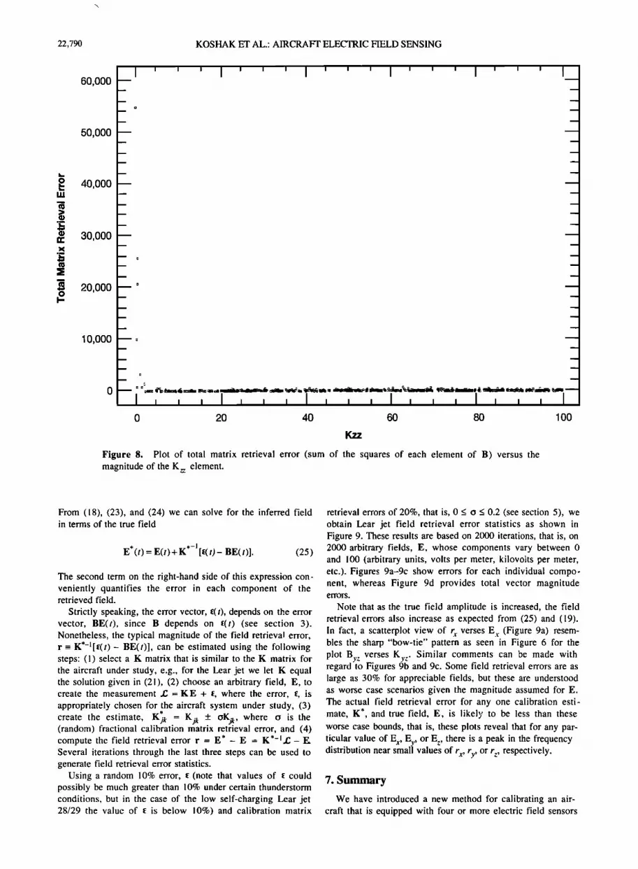
Occasionally there is a large Bjk magnitude, but these large errors are not associated with ill-conditioned K matrices.

Instead, they are associated with matrices that had small values of Kzz as shown in Figure 8 (here the total matrix retrieval error is the sum of the squared elements of B). From (16), multiplication by s I is a very poor correction factor to Kl when K zz is small because K zz I could be retrieved as nearly zero, thereby making s• inordinately large. These large errors are not of practical concern, however, since proper combinations of the aircraft measurements, ap, do not result in exceed- ingly small values of Kzz.

6. Errors in the Inferred Field

In this section, we will clarify exactly how the ambient field is determined and the errors involved. For any arbitrary time t, the ambient field in the aircraft frame of reference E(t) is related to linearly combined aircraft fields œ(t) as in (4)

œ(/)= KE(/) + •(0. (23)

In practice, we will estimate E(t)with E*(t) defined by the linear system

œ (/) = K'E* (t). (24)


60,000

50,000

40,000

30,000

20,000

10,000

,,...

0 20 40 60 80 1 O0

Kzz

Figure 8. Plot of total matrix retrieval error (sum of the squares of each element of B) versus the magnitude of the K,.z element.

From (18), (23), and (24) we can solve for the inferred field in terms of the true field

= K *-1 E*(t) E(t)+ [•(t)- BE(t)]. (25)

The second term on the right-hand side of this expression conveniently quantifies the error in each component of the retrieved field.

Strictly speaking, the error vector, •(t), depends on the error vector, BE(t), since B depends on •(t) (see section 3). Nonetheless, the typical magnitude of the field retrieva! error, r-= K*-l[•(t)- BE(t)], can be estimated using the following steps: (1) select a K matrix that is similar to the K matrix for the aircraft under study, e.g., for the Lear jet we let K equal the solution given in (21), (2) choose an arbitrary field, E, to create the measurement ./2--KE + •, where the error, •, is appropriately chosen for the aircraft system under study, (3)

create the estimate, Kjk --- Kjk _+ OKjk, where o is the (random) fractional calibration matrix retrieval error, and (4) compute the field retrieval error r = E* - E = K*-I.E- E. Several iterations through the last three steps can be used to generate field retrieval error statistics.

Using a random 10% error, • (note that values of • could possibly be much greater than 10% under certain thunderstorm conditions, but in the case of the low self-charging Lear jet 28/29 the value of • is below 10%) and calibration matrix

retrieval errors of 20%, that is, 0 _< o _< 0.2 (see section 5), we obtain Lear jet field retrieval error statistics as shown in Figure 9. These results are based on 2000 iterations, that is, on 2000 arbitrary fields, E, whose components vary between 0 and 100 (arbitrary units, volts per meter, kilovolts per meter, etc.). Figures 9a-9c show errors for each individual component, whereas Figure 9d provides total vector magnitude errors.

Note that as the true field amplitude is increased, the field retrieval errors also increase as expected from (25) and (19).

In fact, a scatterplot view of r x verses E x (Figure 9a) resem- bles the sharp "bow-tie" pattern as seen in Figure 6 for the

plot By z verses K y z. Similar comments can be made with regard to Figures 9b and 9c. Some field retrieval errors are as large as 30% for appreciable fields, but these are understood as worse case scenarios given the magnitude assumed for E. The actual field retrieval error for any one calibration estimate, K*, and true field, E, is likely to be less than these worse case bounds, that is, these plots reveal that for any par-

ticular value of E x, Ey, or E z, there is a peak in the frequency distribution near small values of r x, ry, or rz, respectively.

7. Summary

We have introduced a new method for calibrating an aircraft that is equipped with four or more electric field sensors


• 8 ø g

JequjnN

• o

JequjnN

x

o

o

o

o

o

o

o

o

o

x

o a•

.-o

o

JequJnN

o •

JequJnN

o

o

o

o

o o

o o

N

o

o

o

o

o

o

o

o

o

N


and a high-voltage corona point. We have also suggested a similar calibration procedure for aircraft that are not equipped with a high-voltage corona point and that accumulate little self-charge. We have described our estimate of the aircraft calibration matrix in terms of the true aircraft calibration

matrix and all the errors involved. To explicitly test the calibration procedure and to ascertain calibration matrix retrieval errors, we have applied the method to several known matrices and have simulated all experimental errors. Such a test is the only true mathematical test of any calibration method, since the retrieved matrix can be explicitly compared with the known matrix. We have also applied the method to actual calibration data acquired from a Lear jet 28/29 and found physi- cally consistent results for the ambient fair weather field. Even though this calibration approach helps eliminate the need to estimate aircraft self-charge to infer the ambient vector electric field and reduces calibration errors due to aircraft self-

charge, no calibration method can provide accurate results if the aircraft sensor locations are poorly selected (e.g., placed too close together) or there is excessive aircraft self-charge. Furthermore, the calibration method presented here does not provide explicit values for the aircraft enhancement coefficients, that is, the elements of the M matrix given in (1) above. However, it is noted that these coefficients are not strictly required for retrieving the ambient field. The method also does not provide subsequent estimates of aircraft self- charge during regular data taking periods.

Finally, we have extended the calibration formalism in order to arrive at an explicit form for the retrieved field and associated field retrieval errors (see (25) above). The ambient field retrieval errors are written in terms of the calibration

errors, errors due to aircraft self-charge, electric field sensor measurement errors, and all other errors due to the presence of the aircraft during data taking. We have also demonstrated how the field retrieval error magnitudes can be estimated by use of simulated computer tests.

Appendix: Calibration of an Aircraft With Low Self-Charge and no Available High-Voltage Corona Point

If the aircraft charge, Qp, can be considered small for all pth aircraft calibration maneuvers in fair weather, then we

may redefine ep in (1) to include errors due to aircraft charge,

ap -- MEe + ep, (AI)

where M is now regarded as a (rl x 3) matrix, that is, as given in (1) but with the last column of Q-coefficients removed.

Using the definition in (7), we may write

ap-- •Vlfp + %. (A2)

This equation has the same form as (9) and therefore can be solved in a similar way. We obtain the estimate

Improvements to an initial estimate, •,1 ---1, can be made as described in the text and a final solution of the form M* --

s:zM:z can be found, with, for instance, s:z--al/(•g Mlz 2 ), where a I is the output from the sensor located on the top centerline of the aircraft (sensor location l). In addition, the mathematical form of the retrieved field is similar to (25).

Acknowledgments. This research was supported by the NASA Airborne Field Mill Program (ABFM). Special thanks is given to Mr. Guy Vinson (CSR) for his assistance in the Lear jet calibration. In addition, the help of Launa Maier (NASA Kennedy Space Center), Mark Wheeler (ENSCO), Stephen Tuttle (CSR), and the NASA Langley pilots and flight support crew are greatly appreciated. We also appreciate the data acquisition and weather facilities support at the Cape Canaveral Air Force Station in Florida.

References

Bailey, J. C., and R. V. Anderson, Experimental calibration of a vector electric meter measurement system on an aircraft, NRL Memo. Rep. 5900. Naval Res. Lab., Washington, D.C., March 1987.

Bevington, P. R., Data Reduction and Error Analysis Jbr the Physical Sciences, McGraw-Hill, New York, 1969.

Blakeslee, R. J., H. J. Christian, and B. Vonnegut, Electrical measurements over thunderstorms, J. Geophys. Res., 94, 13135-13140, 1989.

Christian, H. J., J. W. Bullock, C. R. Holmes, W. Gaskell, A. J.

Illingworth, J. Latham, and C. B. Moore, Airborne studies of thunderstorm electrification in New Mexico, in Proceedings in Atmospheric Electricity, pp. 297-300, A. Deepak Publishing, Hampton, VA, 1983.

Gish, O. H., Atmospheric electric observations at Huancayo, Peru, during the solar eclipse, J. Geophys. Res., 49, 123-124, 1944.

Gunn, R., and J. P. Parker, The high-voltage characteristics of aircraft in flight, Proc. IRE, 34, 241-247, 1946.

Jacobson, E. A., and E. P. Krider, Electrostatic field changes produced by Florida lightning, J. Atmos. Sci., 33, 103-117, 1976.

Jones, J. J., Electric charge acquired by airplanes penetrating thunderstorms, J. Geophys. Res., 95, 16589-16600, 1990.

Koshak, W. J., Analysis of lightning field changes produced by Florida thunderstorms, NASA Tech. Memo., TM//103539, 1991.

Kositsky, J., K. L. Giori, R. A. Maffione, D. H. Cronin, and J. E. Nanevicz, Airborne Field Mill (ABFM) System Calibration Report, SRI Proj. 1449, Stanford Res. Inst., Stanford Univ., Stanford, Calif., January, 1991.

Laroche, P., M. Dill, J. F. Gayet, and M. Friedlander, In flight thunderstorm environmental measurements during the Landes 84 cam- paign, paper presented at 10th International Aerospace and Ground Conference on Lightning and Static Electricity, Paris, (dates) 1985.

Twomey, S. A., Introduction to the Mathematics of Inversion in Remote Sensing and Indirect Measurements, Elsevier, New York, 1977.

Winn, W. P., Aircraft measurement of electric field: Self-calibration,

J. Geophys. Res., 98,7351-7365, 1993.

J. Bailey and D. M. Mach, Johnson Research Insititute, University of Alabama, Huntsville, AL 35812.

H. J. Christian and W. J. Koshak, Mail Stop ES43, Marshall Space Flight Center, Huntsville, AL 35812.

(Received February 24, 1993; revised June 21, 1994; accepted June 23, 1994.)

Documents

Aircraft electric field measurements: Calibration and ambient field retrieval