sensors

Article

Aircraft Engine Prognostics Based on InformativeSensor Selection and Adaptive Degradation Modelingwith Functional Principal Component Analysis †

Bin Zhang 1,2, Kai Zheng 1, Qingqing Huang 3,*, Song Feng 1 , Shangqi Zhou 1 and Yi Zhang 1

1 School of Advanced Manufacturing Engineering, Chongqing University of Posts and Telecommunications,Chongqing 400065, China; zhangbin@cqupt.edu.cn (B.Z.); zhengkai@cqupt.edu.cn (K.Z.);fengsong@cqupt.edu.cn (S.F.); zsq11915@163.com (S.Z.); zhangyi@cqupt.edu.cn (Y.Z.)

2 The State Key Laboratory of Mechanical Transmissions, Chongqing University, Chongqing 400044, China3 School of Automation, Chongqing University of Posts and Telecommunications, Chongqing 400065, China* Correspondence: qingq.huang@gmail.com; Tel.: +86-(023)62461709† This paper is an extended version of the paper published in Zhang, B.; Zheng, K.; Luo, J.F.; Zhang, Y.

Informative Sensor Selection and Health Indicator Construction for Aircraft Engines Prognosis. InProceedings of the 2019 International Conference on Sensing, Diagnostics, Prognostics, and Control (SDPC),Beijing, China, 15–17 August 2019. (in press).

Received: 15 December 2019; Accepted: 6 February 2020; Published: 9 February 2020�����������������

Abstract: Engine prognostics are critical to improve safety, reliability, and operational efficiency of anaircraft. With the development in sensor technology, multiple sensors are embedded or deployed tomonitor the health condition of the aircraft engine. Thus, the challenge of engine prognostics liesin how to model and predict future health by appropriate utilization of these sensor information.In this paper, a prognostic approach is developed based on informative sensor selection and adaptivedegradation modeling with functional data analysis. The presented approach selects sensors basedon metrics and constructs health index to characterize engine degradation by fusing the selectedinformative sensors. Next, the engine degradation is adaptively modeled with the functional principalcomponent analysis (FPCA) method and future health is prognosticated using the Bayesian inference.The prognostic approach is applied to run-to-failure data sets of C-MAPSS test-bed developed byNASA. Results show that the proposed method can effectively select the informative sensors andaccurately predict the complex degradation of the aircraft engine.

Keywords: prognostics; aircraft engine; sensor selection; degradation modeling; functional principalcomponent analysis; Bayesian inference

1. Introduction

As the heart of an aircraft, the engine consists of several subsystems with millions of parts, and itshealth condition directly impacts operation and safety of the whole aircraft system. While the reliabilityof aero-engines has been improved over the years, factors such as fatigue and wear will inevitablycause the health condition of an engine to degrade with usage, reducing the overall performance ofthe powered aircraft [1]. Therefore, a number of sensors of varying types have been widely usedto monitor the health degradation of aircraft engines, which creates a multi-sensor environment foroperational health analysis and maintenance decision-making. Over the past decades, prognostics thatutilizes monitoring sensors information to predict the future health and estimates the remaining usefullife (RUL) before failure/end-of-life has attracted increasing attention from academic researchers andindustrial operators [2]. For its potential in enhancing reliability and maintenance efficiency while

Sensors 2020, 20, 920; doi:10.3390/s20030920 www.mdpi.com/journal/sensors

Sensors 2020, 20, 920 2 of 21

reducing unnecessary maintenance and minimizing operational costs, prognostics have been an activeresearch field for aircraft engine applications [3].

Generally, the existing methods pertaining to aircraft engine prognostics can be classified into twocategories: model-based and data-driven methods. For model-based methods, a mathematical modelthat can describe the engine health degradation process that is normally required to be constructedaccording to physical failure characteristics before prediction. Some typical model-based methods havebeen developed for engine health estimation and RUL prediction, such as the Markov model-based [4,5]and particle filtering-based method [6,7]. While model-based methods enable improved accuracyof engine prognostics, certain assumptions and simplifications of the adopted models may poselimitations on their practical deployment. With the rapid development of data mining techniques andthe growing availability of health monitoring data, data-driven methods attract increasing attention.Data-driven methods utilize the information extracted or learned from observed data to identify thedegradation behavior and predict the future health condition without using any particular physicalmodel [8,9]. In this view, data-driven methods may be the more applicable prognostic solution forcomplicated systems, as aero-engines that have limited knowledge of physics-of-failure but havemassive multi-sensor monitoring data. Among the data-driven prognostic methods, machine learningand statistical approaches are two popular branches. The common machine learning techniques usedfor prognostics include support vector regression [10], artificial neural network [11,12], fuzzy logic [13],etc. Machine learning methods are capable of dealing with prognostic issues of complex systems,but the predicted results are hard to be explained because of the lack of transparency. Besides, it isdifficult for machine learning methods to handle the uncertainty in health degradation and long-termprognostics. In contrast, statistical approaches fit probabilistic models to the health monitoring dataand are effective in managing the uncertainty of the degradation process as well as its influence onfuture predictions. Thus, statistical prognostics are recently becoming dominant [2].

In statistical data driven prognostics, the available health monitoring data that contains usefulhealth degradation information is modeled by statistical models to perform prognostics [14]. Initially,regression-based statistical models are applied to model the available data and predict future health.In [15], a hybrid multi-variate adaptive regression splines method was proposed for the aircraft engineprognosis. To account unit-to-unit variability, Zaidan et al. [16] formulated a Bayesian hierarchicalmodel with linear random coefficient model for engine prognostics. A parametric pth order polynomialmodel was proposed by Liu et al. [17,18] and was validated on a degradation dataset of an aircraftgas turbine engine. Another group of frequently used statistical models are stochastic process modelsthat can well capture the degradation dynamics of a system. For its nice mathematical properties,the Wiener process has been intensively studied in degradation modeling and prognostics for enginesand other engineered systems [19]. Considering monotone non-decreasing degradation in practice,Le Son et al. [20] modeled deterioration of gas turbine engines as a non-homogeneous Gamma process.Peng et al. [21] further researched modeling of time-varying degradation rates with an inverse Gaussianprocess. In practice, statistical approaches are mainly concentrated on univariate degradation modelingand prognostics, so a composite health index (HI) that captures health degradation of an engine isnormally needed to be constructed by fusion of the multi-sensor monitoring data. Wang et al. [22]proposed a HI construction method by a linear data transformation method of multi-sensor data.In [23], the failure time and the multi-sensor data are combined via a novel latent linear model toconstruct a generic HI. Theoretically, integration of more sensors may be beneficial for prognostics.However, different sensors usually have different levels of relevance to the degradation process. Also,some sensors may be even unrelated to the underlying degradation process due to high noise, lowsensitivity to the health degradation, inconsistency among the population, etc. In addition, fusion oftoo many sensors may incur a heavy data processing burden and unnecessary costs. As a result, it isbetter to select the degradation-relevant sensors for HI construction, and hereafter, this kind of sensorsare denoted as informative sensors in this paper. Coble et al. [24] proposed three metrics to characterizethe suitability of sensors for prognostics. Yu [6] proposed an informative sensor selection method

Sensors 2020, 20, 920 3 of 21

based on logistic regression with penalization regularization for aircraft engine health prognostics.In [25], Liu et al. proposed an improved permutation entropy method for selection of informativesensors. To identify multiple stages before failure, Chehade et al. studied informative sensor selectionand fusion using statistical hypothesis testing [26]. Besides, the task of informative sensor selectionwas integrated with the statistical modeling in [23] and [27] for engine prognostics.

Through fusion of the selected informative sensors into a composite HI, many statistical methodshave been proposed for prognostics of complex systems, including aircraft engines. However, most ofthe statistical approaches are based on parametric models, such as a linear model [16,23,28], exponentialmodel [17,27], quadratic model [24], etc. These methods are effective when the engine degradationpattern can be described with a specific model, but there are numerous cases where the degradationtrajectory may not be appropriately fitted by a parametric model [1,3,16]. Therefore, a more flexibledegradation modeling and prognosis technique is needed for practical applications. Furthermore,the existing literature relevant to the selection of informative sensors is basically focused on therelevance of a sensor to the degradation process. While metrics of monotonicity [10,25], correlationand robustness [2,29] have been commonly utilized to evaluate the relevance of sensors for prognostics.There is a lack of efforts to consider the degree to which the sensors of a population of systems havethe same underlying shape [24]. Specifically, for a fleet of engines operating under one operationalcondition and with one failure mode, it is highly desired that the sensor demonstrating a consistentlyincreasing or decreasing trend for all the engines to be selected as the informative sensor. To addressthese limitations, a statistical method with informative sensor selection is proposed for prognostics ofthe aircraft engine in this paper. In the presented method, a new metric that evaluates the degree ofconsistent trend of a sensor for a population of systems is proposed and used to select informativesensors to construct the engine HI. Then, the functional principal component analysis (FPCA) method isapplied to adaptively model the engine HI and combined with Bayesian inference for future prognostics.

The remainder of this paper is organized as follows. Section 2 briefly gives the related theories.Section 3 presents a detailed description of the proposed prognostic approach. Section 4 demonstratesthe developed method with a case study on the degradation of a turbofan engine. Section 5 discussessome key issues of the proposed approach. Finally, Section 6 summaries the research and future work.

2. Related Theories

In this section, the theories utilized in this study are briefly introduced.

2.1. Basics of FPCA

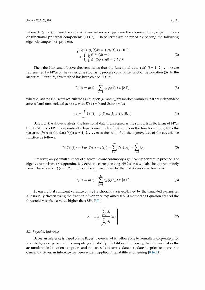
Functional data analysis concerns the analysis of data that are in the form of a function withstatistical methods. Functional data are of intrinsically infinite dimension, and thus, dimensionreduction based on some kind of basis function is crucial for analysis of such data. Unlike theparametric basis function such as B-spline, Fourier, and wavelet functions, FPCA directly derives thebasis function from the data and has been a useful tool for functional data analysis [30–32].

In functional data analysis, the given data Yi(t) (i = 1, 2, . . . , n) is assumed as an independentand identically distributed (i.i.d) realization of a stochastic process Y(t) that is in L2 and defined onthe interval [0, Γ]. The expectation and covariance function of Y(t) are respectively µ(t) = E(Y(t)) andG(s, t) = E((Y(s) − µ(s))(Y(t) − µ(t))), where E(·) is the expectation operator. Under mild assumptions,Mercer’s theorem implies that the spectral decomposition of G(s, t) leads to:

G(s, t) =∞∑

k=1

λkφk(s)φk(t), t ∈ [0, Γ] (1)

Sensors 2020, 20, 920 4 of 21

where λ1 ≥ λ2 ≥ ... are the ordered eigenvalues and φk(t) are the corresponding eigenfunctionsor functional principal components (FPCs). These terms are obtained by solving the followingeigen-decomposition problem: ∫

Γ G(s, t)φk(t)ds = λkφk(t), t ∈ [0, Γ]

s.t.{ ∫

Γ φk2(t)dt = 1∫

Γ φl(t)φk(t)dt = 0, l , k(2)

Then the Karhunen–Loève theorem states that the functional data Yi(t) (i = 1, 2, . . . , n) arerepresented by FPCs of the underlying stochastic process covariance function as Equation (3). In thestatistical literature, this method has been coined FPCA:

Yi(t) = µ(t) +∞∑

k=1

εikφk(t), t ∈ [0, Γ] (3)

where εik are the FPC scores calculated as Equation (4), and εik are random variables that are independentacross i and uncorrelated across k with E(εik) = 0 and E(εik

2) = λk:

εik =

∫Γ(Yi(t) − µ(t))φk(t)dt, t ∈ [0, Γ] (4)

Based on the above analysis, the functional data is expressed as the sum of infinite terms of FPCsby FPCA. Each FPC independently depicts one mode of variations in the functional data, thus thevariance (Var) of the data Yi(t) (i = 1, 2, . . . , n) is the sum of all the eigenvalues of the covariancefunction as follows:

Var(Yi(t)) = Var(Yi(t) − µ(t)) =∞∑

k=1

Var(εik) =∞∑

k=1

λik (5)

However, only a small number of eigenvalues are commonly significantly nonzero in practice. Foreigenvalues which are approximately zero, the corresponding FPC scores will also be approximatelyzero. Therefore, Yi(t) (i = 1, 2, . . . , n) can be approximated by the first K-truncated terms as:

Yi(t) = µ(t) +K∑

k=1

εikφk(t), t ∈ [0, Γ] (6)

To ensure that sufficient variance of the functional data is explained by the truncated expansion,K is usually chosen using the fraction of variance explained (FVE) method as Equation (7) and thethreshold η is often a value higher than 85% [30]:

K = mink

k∑

i=1λi

∞∑i=1

λi

≥ η

(7)

2.2. Bayesian Inference

Bayesian inference is based on the Bayes’ theorem, which allows one to formally incorporate priorknowledge or experience into computing statistical probabilities. In this way, the inference takes theaccumulated information as a priori, and then uses the observed data to update the priori to a posterior.Currently, Bayesian inference has been widely applied in reliability engineering [8,16,21].

Sensors 2020, 20, 920 5 of 21

For a continuous random variable y and related random parameters θ, Bayes’ theorem states thattheir joint probability can be written in two ways as [33]:

p(θ, y) = p(y |θ )p(θ) = p(θ∣∣∣y )

p(y) (8)

Eliminating the joint probability p(y, θ) and rearranging a bit, we obtain Bayesian inference forthe parameters θ:

p(θ∣∣∣y )

=p(y |θ )p(θ)

p(y)∝ p(y |θ )p(θ) (9)

In the literature, p(θ|y) and p(θ) are respectively defined as the posterior and prior distributionof the random parameters θ, and p(y|θ) is denoted as the likelihood function. The p(y|θ) can beunderstood as the probability of observing samples of the random variable y conditioned on theparameters θ. Based on Equation (9), Bayesian inference updates the parameters distribution from apriori to a posterior with the likelihood function of the observed data. Thus, the uncertainty in theparameters can be reduced and accuracy of further inference using the parameters can be improved.

3. The Proposed Method

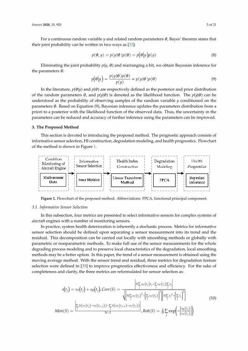
This section is devoted to introducing the proposed method. The prognostic approach consists ofinformative sensor selection, HI construction, degradation modeling, and health prognostics. Flowchartof the method is shown in Figure 1.

Sensors 2020, 20, x 5 of 22

To ensure that sufficient variance of the functional data is explained by the truncated expansion, K is usually chosen using the fraction of variance explained (FVE) method as Equation (7) and the threshold η is often a value higher than 85% [30]:

1

1

min

k

ii

k

ii

Kλ

ηλ

=∞

=

= ≥

(7)

2.2. Bayesian Inference

Bayesian inference is based on the Bayes’ theorem, which allows one to formally incorporate prior knowledge or experience into computing statistical probabilities. In this way, the inference takes the accumulated information as a priori, and then uses the observed data to update the priori to a posterior. Currently, Bayesian inference has been widely applied in reliability engineering [8,16,21].

For a continuous random variable y and related random parameters θ, Bayes’ theorem states that their joint probability can be written in two ways as [33]:

( ) ( ) ( ) ( ) ( ),p y p y p p y p y= =θ θ θ θ (8)

Eliminating the joint probability p(y, θ) and rearranging a bit, we obtain Bayesian inference for the parameters θ:

( ) ( ) ( )( ) ( ) ( )

p y pp y p y p

p y= ∝

θ θθ θ θ (9)

In the literature, p(θ|y) and p(θ) are respectively defined as the posterior and prior distribution of the random parameters θ, and p(y|θ) is denoted as the likelihood function. The p(y|θ) can be understood as the probability of observing samples of the random variable y conditioned on the parameters θ. Based on Equation (9), Bayesian inference updates the parameters distribution from a priori to a posterior with the likelihood function of the observed data. Thus, the uncertainty in the parameters can be reduced and accuracy of further inference using the parameters can be improved.

3. The Proposed Method

This section is devoted to introducing the proposed method. The prognostic approach consists of informative sensor selection, HI construction, degradation modeling, and health prognostics. Flowchart of the method is shown in Figure 1.

Figure 1. Flowchart of the proposed method. Abbreviations: FPCA, functional principal component.

Figure 1. Flowchart of the proposed method. Abbreviations: FPCA, functional principal component.

3.1. Informative Sensor Selection

In this subsection, four metrics are presented to select informative sensors for complex systems ofaircraft engines with a number of monitoring sensors.

In practice, system health deterioration is inherently a stochastic process. Metrics for informativesensor selection should be defined upon separating a sensor measurement into its trend and theresidual. This decomposition can be carried out locally with smoothing methods or globally withparametric or nonparametric methods. To make full use of the sensor measurements for the wholedegrading process modeling and to preserve local characteristics of the degradation, local smoothingmethods may be a better option. In this paper, the trend of a sensor measurement is obtained using themoving average method. With the sensor trend and residual, three metrics for degradation featureselection were defined in [29] to improve prognostics effectiveness and efficiency. For the sake ofcompleteness and clarity, the three metrics are reformulated for sensor selection as:

s(t j)= sT

(t j)+ sR

(t j), Corr(S) =

∣∣∣∣∣∣∣N∑j

sT(t j)t j−∑j

sT(t j)∑j

t j

∣∣∣∣∣∣∣√√N∑j

sT(t j)2−

∑j

sT(t j)2

N∑j

t j2−

∑j

t j

2Mon(S) =

∣∣∣∣∣∣∣∑jδ(sT(t j)−sT(t j−1))−

∑jδ(sT(t j−1)−sT(t j))

∣∣∣∣∣∣∣N−1 , Rob(S) = 1

N∑j

exp(−

∣∣∣∣∣ sR(t j)sT(t j)

∣∣∣∣∣)(10)

Sensors 2020, 20, 920 6 of 21

where s(tj) is the measurement of the sensor S at the time tj (j = 1, 2, . . . , Nj) with the trend of sT(tj) andresidual sR(tj), δ(·) is the simple unit step function.

Among the three metrics, correlation (Corr) measures the linearity between the interested sensorand the usage time, monotonicity (Mon) assesses consistently increasing or decreasing trend of thesensor, and robustness (Rob) reflects the tolerance of the sensor to noises and outliers. The sensorwith higher scores should be selected as the informative sensor, for the three metrics are all positivelycorrelated with the relevance of a sensor to the system degradation.

From Equation (10), it can be concluded that these metrics are defined on the sensor from oneindividual system and the same sensor from other systems of the population is not accounted. Fora population of systems (such as a group of aircraft engines) that operate under the same conditionand with one failure mode, the informative sensor is highly desired to have a consistent increasing ordecreasing trend for all the systems. Additionally, the sensor with a small variation of measurementsupon system failures and a large range till failure is also desired for prognostics. Thus, a new metric ofpredictability (Pre) is formulated for sensor selection as:

Pre(S) = Exp

− std(s f

)∣∣∣∣mean(s f

)−mean(ss)

∣∣∣∣ (11)

where sf and ss are respectively the measurements at the failure and start instant of the sensor S for apopulation of systems.

The new metric Pre takes the failure and start values of a sensor from the entire population intoaccount, and thus the trend consistency of a sensor among a population is given consideration. Also,Pre is positively related to the performance of the sensor with the range of [0,1], and favorites thesensor with well-clustered failure values and large range. That is the sensor with a high score of Preshould be selected as the informative sensor.

For prognostic parameter selection, Coble et al. presented three metrics in [24] and theprognosability (Pro) metric is quite similar to the proposed Pre. However, the two metrics aredifferent in measuring the range of one sensor. In the metric Pro, the range is the mean range fromstart to failure for a population of systems. Sensors with well-clustered failure values and large rangeare encouraged by this measure. While in the Pre, as in Equation (11), the sensor measurements at thestart and failure instant of a population are respectively averaged to the given range of the sensor. Themetric Pre selects sensors with both well-clustered failure and start values as well as large range.

To select the informative sensor for aircraft engines, two steps are included using the presentedgoodness metrics. In the first step, binary-value and constant-value sensors are eliminated by simplevisual inspection, because these sensors do not make sense for prognosis. As can be seen from thesedefinitions, one goodness metric only partially measures suitability of a sensor for prediction andsensor selection based on only one metric will be biased. In the second step, sensors are evaluatedby four metrics simultaneously, and then the informative sensors selected with drop out strategy arefused to construct a HI for health prognosis of aircraft engines.

3.2. Health Index Construction

For a data-driven prognostics, extraction of the health signatures and background knowledgefrom massive training/testing sensors is required. Based on the selected informative sensors, the HIconstruction is considered in this subsection.

The transformation of the selected informative sensors into one-dimensional HI is a processof information fusion, which enables a general measure to characterize the health condition of asystem and also the degradation of different systems from the same population to be similar. TheHI can be constructed using many information fusion techniques, such as linear data transformationmethod [13,17,22], PCA and Euclidean distance measure [20], and logistic regression [6,11]. For its

Sensors 2020, 20, 920 7 of 21

effectiveness and ease of use, the linear data transformation method is also employed to construct theHI for aero-engines in this paper.

Suppose the selected informative sensors are d-dimensional and the two sensor data sets thatrepresent the aircraft engine failed, and healthy states are Q0 of M0 × d and Q1 of M1 × d matrix, whereM0 and M1 are, respectively, the data sizes for engine failed and healthy states. Generally, data sets forhealthy and failed states can be collected from the training data sets at the beginning and at the end ofthe run-to-failure tests. With these two data sets, a transformation matrix T of d × 1 is obtained andthen the one-dimensional HI y for any d-dimensional matrix Q is:

y = QTT = (Qo f f

TQo f f )−1Qo f f

TSo f f(12)

where Qoff = [Q0; Q1]T, Soff = [S0, S1]T, S0 is a 1 ×M0 zero vector and S1 is a 1 ×M1 unity vector.As can be easily derived, the HI obtained by the linear transformation method as Equation (12) is

varying approximately between 1 and 0. With the usage of the aircraft engine, the HI has a decreasingtrend. This HI contains health condition information extracted from multi-dimensional informativesensors of the monitored aircraft engine. It can be used to construct background health knowledgein the offline process and to further conduct the online prediction process. Although the lineartransformation is discussed here and will be employed for the case studies, other information fusionmethods can also be used to construct the HI with the selected informative sensors.

3.3. Degradation Modeling by FPCA

In view that the health degradation is a stochastic process with uncertainties from physicaldegradation dynamics, usage variations and other effects, the degradation pattern of an aircraft engineis complex and unknown. To adaptively study the aircraft engine degradation, the HI that describesthe health deterioration of an engine is assumed as discrete sampling values of the functional data andis modeled with the FPCA method in this subsection.

Suppose there is a population of aircraft engines, then the degradation pattern of one aircraftengine is an independent realization of the degradation process of the whole population. Based on theFPCA analysis method briefly introduced in Section 2, the degradation of one engine can be representedby the mean function and FPCs derived adaptively from the population stochastic degradation processX(t) (t∈I), where I is the service time interval of the population of engines (the observation interval forthe engine/system with the longest possible lifetime). Further, considering the fact that the HI indirectlydemonstrates the health degradation of the engine, so the measurement error is one important aspectthat should be accounted for. To be specific, for a population of n aircraft engines with Ni measurementsfor the i-th engine, the degradation of the i-th engine is modeled with its HI yi(tij) (i = 1, 2, . . . , n; j = 1,2, . . . , Ni) by FPCA as:

yi(ti j

)= xi

(ti j

)+ ei j

xi(t) = µ(t) +K∑

k=1εikφk(t)

(13)

where xi(tij) and eij are the unobservable degradation and measurement error of the i-th engine at timetij, xi(t) is the underlying functional data with the mean function µ(t) and the FPCs φk(t)s for the i-thengine, and εik are the related FPC scores.

With the FPCA-based degradation modeling as Equation (13), the degradation characteristicsof the whole engine population is represented by the mean function and the first K FPCs, whilethe degradation peculiarity of an engine is captured by its specific FPC scores. The mean functionµ(t) describes the common degradating trend of all the engines from an engine population, and thefirst few FPCs reflect the main varying modes of the population degradation process. As in [27,34],the measurement errors eij are practically assumed to be i.i.d with the normal distribution N(0, σ2) andare also independent of FPC scores in this study. Also, note that no pre-specified parametric form is

Sensors 2020, 20, 920 8 of 21

needed to be assumed for µ(t) and the φk(t)s, but they are adaptively derived from the engines HI inthe following.

For the mean function µ(t) = E(X(t)), it is estimated by local linear smoothers using degradationobservations yi(tij) (i = 1, 2, . . . , n; j = 1, 2, . . . , Ni) from all n engines as:

µ(t) = α0(t)

minα0,α1

∑i

∑jκ1

(ti j−thµ

)(yi(ti j

)− α0 − α1

(t− ti j

))2 (14)

where κ1(·) is a univariate kernel function and hµ is the smoothing bandwidth.For estimations of the φk(t)s, the covariance function G(s, t) = E((X(s) − µ(s))(X(t) − µ(t))) of the

engine degradation process X(t) should be firstly estimated. For the n engines, the following holds:

Vi(ti j, til

)=

(yi(ti j

)− µ

(ti j

))(yi(til) − µ(til))

E(Vi

(ti j, til

))= V

(ti j, til

)= G

(ti j, til

)+ σ2δ jl

(15)

where δij is the Kronecker delta function.It is easy to see that the diagonal (i.e., j = l) of the raw covariance function V(tij, til) calculated with

the degradation observations are contaminated with measurement errors. Estimation of the covariancefunction G(s, t) using the local linear surface smoothing should be without the diagonal as:

G(s, t) = β0(s, t)

minβ0,β11,β12

∑i

∑1≤ j,l≤Ni

κ2

(ti j−shG

, til−thG

)(Vi

(ti j, til

)− β0 − β11

(s− ti j

)− β12(t− til)

)2 (16)

where κ2(·) is a bivariate kernel function and hG is the smoothing bandwidth.Then eigen-decomposition following Equation (2) by discretizing the G(s, t) is performed to obtain

the eigenvalues λk (k = 1, 2, . . . ) and the corresponding FPCs. Spline interpolation is further utilizedto obtain the continuous φk(t)s.

For the variance σ2 of the measurement errors, it is related to the diagonal values of V(tij, til) andG(s, t). To mitigate boundary effects, its estimation is:

σ2 = max(

2I

∫I1

(V(t) − G(t)

)dt, 0

)(17)

where V(t) is the local linear smoother of diagonal values of V(tij, til), G(t) is the diagonal values ofG(s, t), and the interval I1 = [I/4, 3I/4].

Considering the measurement errors in the degradation model, to estimate FPC scores withEquation (4) will lead to bias. To remedy that, the conditional expectation method proposed byYao et al. [35] is utilized here to estimate the εik:

εik = λkφTik

^Σ

−1

i (yi − µi) (18)

where yi = (yi1, yi2, ..., yiNi)T is the engine HI observing vector, µi = (µi1, µi2, . . . , µiNi)T and φiκ =(

φi1, φi2, . . . , φiNi)T

are the mean and FPC vectors interpolated from the mean function and FPCs, and^Σi is with the entry (j, l) as

^Σi( j, l) = G

(ti j, til

)+ σ2δ jl.

With the estimated parameters, the uncontaminated degradation of the i-th engine is modeled byFPCA as:

xi(ti j

)= µ

(ti j

)+

K∑k=1

εikφk(ti j

)(19)

Sensors 2020, 20, 920 9 of 21

Based on the FPCA modeling analysis, degradation of an engine is statistically represented withthe common trend and a few varying terms that reflect the main dynamics of the degradation process.For estimation of the model parameters, all degradation observations of the engine population arefused and local linear smoothing is needed. In this study, the Gaussian kernel function is appliedfor both curve and surface smoother, and the related smoothing bandwidth is determined by theone-leave-out cross-validation strategy.

3.4. Prognostics with Bayesian Inference

For one aero-engine that is still operating, its future health is of significance for condition-basedmaintenance and health management. Therefore, Bayesian inference is combined with the degradationmodel for engine prognostics in this Subsection.

With the degradation modeling by FPCA as detailed in the previous Subsection, the degradationtrajectory of one in-service engine can be described as:

x(t) = µ(t) +K∑

k=1

εkφk(t) (20)

Assume that we have monitored the in-service engine at a vector of time t = (t1, t2, ..., tH) withthe observed HI y1:H = (y1, y2, ..., yH)T, where tH denotes the latest monitoring time. Once the meanfunction µ(t) and FPCs φk(t)s are estimated with HI of historical run-to-failure engines of the populationas elaborated in Section 3.3, the trend and the main variations of the in-service engine degradation canbe obtained by interpolations with its monitoring times. However, the FPC scores ε = (ε1, ε2, ..., εK)T

are to be inferenced.In practice, system health deterioration is usually a gradual process under the effects of various

internal and external environmental factors, and the degradation process can be assumed as aGaussian process. Then the uncorrelated FPC scores εk (k = 1, 2, ..., K) will respectively follow thenormal distributions N(0, λk) with λk being the ordered eigenvalues of the covariance function of thedegradation process. Taking FPC scores estimated from the historical run-to-failure engines as the priordistribution p0(ε) and considering the likelihood function p(y1:H |ε) of observing y1:H [36], we have:

p0(ε) ∼ N(0, Λ), Λ = diag(λ1, λ2, . . . , λK

)p(y1:H |ε ) =

1√

2πσ2exp

(−

eTe2σ2

), e = y1:H − µ1:H −Φε

(21)

where µ1:H and Φ with entry (h, k) as φk(th) (h = 1, 2, . . . , H; k = 1, 2, . . . , K) are respectivelyinterpolated with the monitoring time vector t = (t1, t2, ..., tH) from the µ(t) and φk(t)s estimated fromthe run-to-failure engines, and σ2 is the estimated measurement error.

Based on Bayesian inference outlined in Section 2.2, the posterior distribution p(ε|y1:H) of the FPCscores ε of the in-service engine can be updated as:

p(ε∣∣∣y1:H

)∝ p0(ε)p(y1:H |ε ) (22)

From Equation (21), the p0(ε) and p(y1:H |ε) are conjugate multivariate normal distributions. Thep(ε|y1:H) can be analytically derived to also follow multivariate normal distribution as follows:

p(ε∣∣∣y1:H

)∼ N

(µεH, Σε

H

)Σε

H =(

ΦTΦσ2 + Λ−1

)−1,µεH = Σε

HΦT

σ2 (y1:H − µ1:H)(23)

Sensors 2020, 20, 920 10 of 21

Further inserting the posteriori distribution of the FPC scores ε into Equation (20), a real-timeprognosis for the in-service engine based on the latest observations y1: H is:

x(t) ∼ N(µx

H(t), σ2xH (t)

)µx

H(t) = µ(t) +φT(t)µεH, σ2xH (t) = φT(t)Σε

Hφ(t)(24)

where µ(t) = µ(t) and φ(t) =(φ1(t), φ2(t), . . . , φK(t)

)Tare respectively the mean value and FPC

vector interpolated from the mean function and K FPCs at a future time t.

4. Case Studies and Results Analysis

The main purpose of this section is to demonstrate the validity and performance of the proposedprognostics approach with the case study on an aircraft gas turbine engine.

4.1. Sensor Data of Aircraft Engine

The sensor data of the aircraft gas turbine engine degradation is generated from the commercialmodular aero-propulsion system simulation (C-MAPSS) developed at NASA [37] and published onlinefor research investigations. Each time series signal represents a different degradation instance of thedynamic simulation of the same engine population and consists of multi-sensor measurements. Foreach cycle of a degradation instance, 21 sensor measurements, as listed in Table 1, were recorded.The multi-sensor data was contaminated with noises and each engine started with different initialhealth conditions and manufacturing variations, which was unknown. With limited knowledgeabout the true physical model, we relied solely on the multi-sensor data from the training and testingengines to understand the engine degradation process. The data can be downloaded from NASA datarepository [38].

In particular, the data set FD001 that contains 100 training and testing engines is used in thisstudy. The multi-sensor measurements for each training engine were collected until failure, whereasthe multi-sensor measurements for each in-service unit were truncated at some random point beforeits failure. Although these engines were simulated under one operational condition and one failuremode, the engine with multiple usage conditions and failure modes may also be analyzed using theproposed method with necessary processing as in [20,39].

Sensors 2020, 20, 920 11 of 21

Table 1. Sensor measurements of the aircraft engine.

Symbol Description Units

T2 Total temperature at fan inlet ◦RT24 Total temperature at LPC outlet ◦RT30 Total temperature at HPC outlet ◦RT50 Total temperature at LPT outlet ◦RP2 Pressure at fan inlet Psia

P15 Total pressure in bypass-duct PsiaP30 Total pressure at HPC outlet PsiaNf Physical fan speed RpmNc Physical core speed Rpmepr Engine pressure ratio (P50/P2) –

Ps30 Static pressure at HPC outlet Psiaphi Ratio of fuel flow to Ps30 pps/psiNRf Corrected fan speed RpmNRc Corrected core speed RpmBPR Bypass Ratio –farB Burner fuel-air ratio –

htBleed Bleed Enthalpy –Nf_dmd Demanded fan speed Rpm

PCNfR_dmd Demanded corrected fan speed RpmW31 HPT coolant bleed lbm/sW32 LPT coolant bleed lbm/s

4.2. Results and Analysis on Informative Sensor Selection

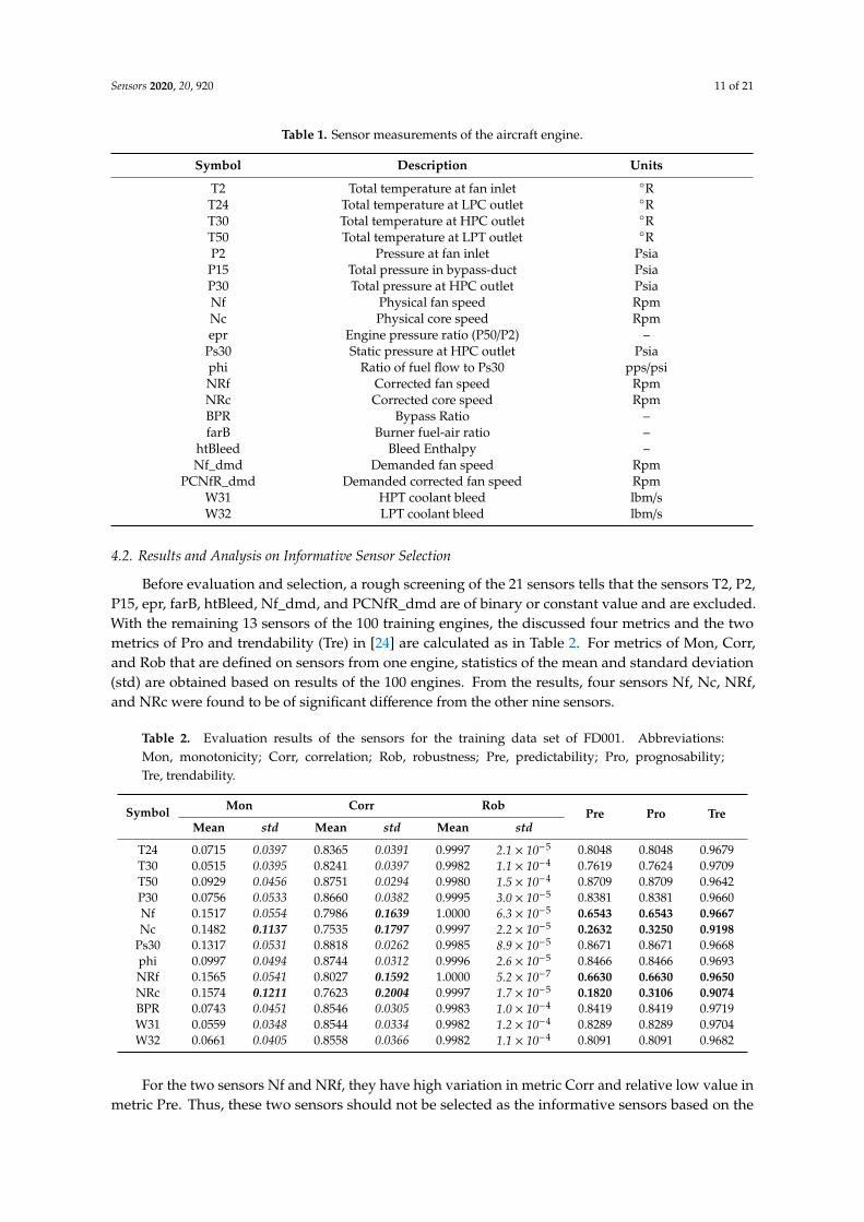
Before evaluation and selection, a rough screening of the 21 sensors tells that the sensors T2, P2,P15, epr, farB, htBleed, Nf_dmd, and PCNfR_dmd are of binary or constant value and are excluded.With the remaining 13 sensors of the 100 training engines, the discussed four metrics and the twometrics of Pro and trendability (Tre) in [24] are calculated as in Table 2. For metrics of Mon, Corr,and Rob that are defined on sensors from one engine, statistics of the mean and standard deviation(std) are obtained based on results of the 100 engines. From the results, four sensors Nf, Nc, NRf,and NRc were found to be of significant difference from the other nine sensors.

Table 2. Evaluation results of the sensors for the training data set of FD001. Abbreviations:Mon, monotonicity; Corr, correlation; Rob, robustness; Pre, predictability; Pro, prognosability;Tre, trendability.

Symbol Mon Corr RobPre Pro Tre

Mean std Mean std Mean std

T24 0.0715 0.0397 0.8365 0.0391 0.9997 2.1 × 10−5 0.8048 0.8048 0.9679T30 0.0515 0.0395 0.8241 0.0397 0.9982 1.1 × 10−4 0.7619 0.7624 0.9709T50 0.0929 0.0456 0.8751 0.0294 0.9980 1.5 × 10−4 0.8709 0.8709 0.9642P30 0.0756 0.0533 0.8660 0.0382 0.9995 3.0 × 10−5 0.8381 0.8381 0.9660Nf 0.1517 0.0554 0.7986 0.1639 1.0000 6.3 × 10−5 0.6543 0.6543 0.9667Nc 0.1482 0.1137 0.7535 0.1797 0.9997 2.2 × 10−5 0.2632 0.3250 0.9198

Ps30 0.1317 0.0531 0.8818 0.0262 0.9985 8.9 × 10−5 0.8671 0.8671 0.9668phi 0.0997 0.0494 0.8744 0.0312 0.9996 2.6 × 10−5 0.8466 0.8466 0.9693NRf 0.1565 0.0541 0.8027 0.1592 1.0000 5.2 × 10−7 0.6630 0.6630 0.9650NRc 0.1574 0.1211 0.7623 0.2004 0.9997 1.7 × 10−5 0.1820 0.3106 0.9074BPR 0.0743 0.0451 0.8546 0.0305 0.9983 1.0 × 10−4 0.8419 0.8419 0.9719W31 0.0559 0.0348 0.8544 0.0334 0.9982 1.2 × 10−4 0.8289 0.8289 0.9704W32 0.0661 0.0405 0.8558 0.0366 0.9982 1.1 × 10−4 0.8091 0.8091 0.9682

For the two sensors Nf and NRf, they have high variation in metric Corr and relative low value inmetric Pre. Thus, these two sensors should not be selected as the informative sensors based on the

Sensors 2020, 20, 920 12 of 21

analysis in Section 3.1. In addition, the two sensors score low values of metric Pro proposed in [24],verifying the effectiveness of the proposed metric Pre. Nevertheless, the metric Tre proposed alsoin [24] to characterize the trendability of a population of sensors scores both high for the two sensors.To make sense of interpretation, signals of the two sensors for the 100 training engines are shownin Figure 2. It shows that the two sensors are not correlated well with the usage of the engine andtheir ranges are both very small (actually less than 0.5) from start to failure, which validates thesesensors have high variation in metric Corr and score low value in metric Pre and Pro. In previousstudies using the C-MAPSS data, including [9,20], the above two sensors were also wiped out asnon-informative sensors.

Sensors 2020, 20, x 13 of 22

0 50 100 150 200 250 300 350 4002387.7

2387.8

2387.9

2388

2388.1

2388.2

2388.3

2388.4

2388.5

2388.6

0 50 100 150 200 250 300 350 4002387.7

2387.8

2387.9

2388

2388.1

2388.2

2388.3

2388.4

2388.5

2388.6

(a) (b)

Figure 2. Sensor signals for the 100 training engines: (a) Nf; (b) NRf.

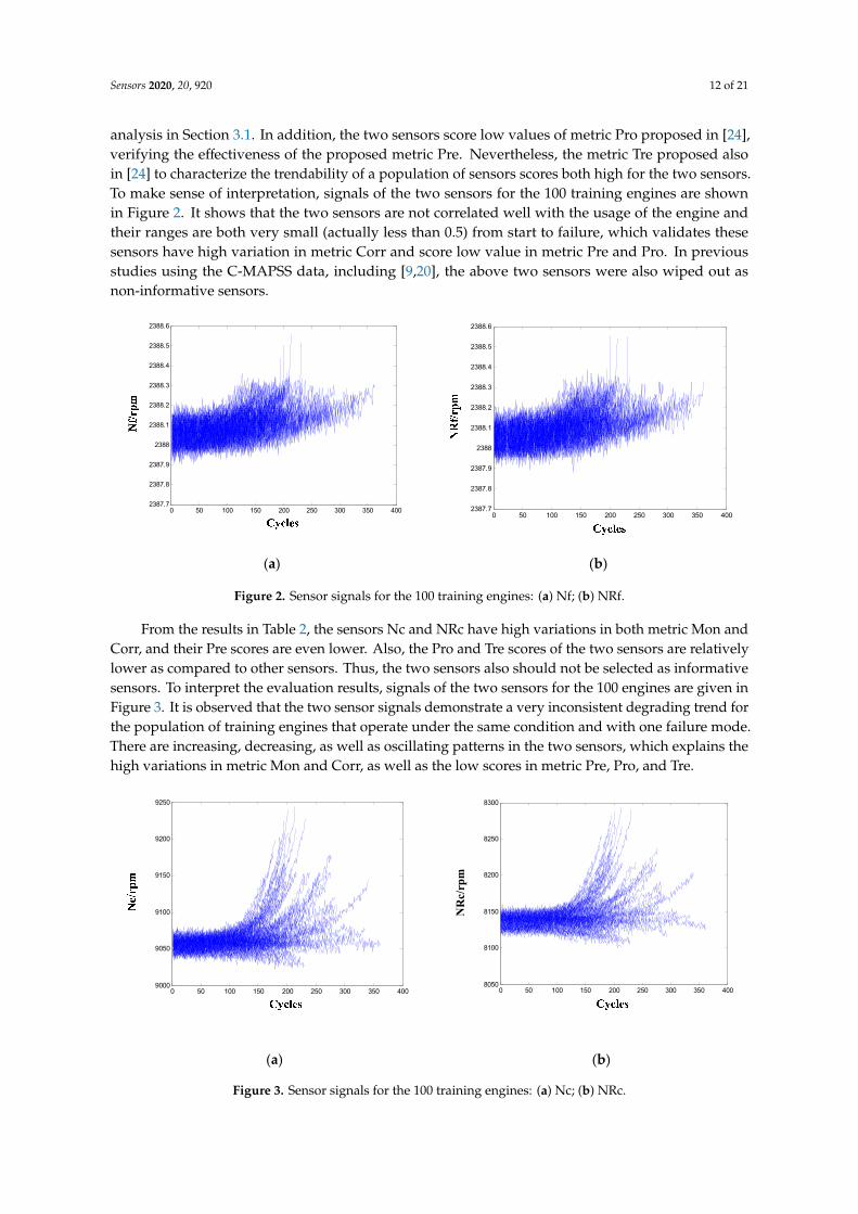
From the results in Table 2, the sensors Nc and NRc have high variations in both metric Mon and Corr, and their Pre scores are even lower. Also, the Pro and Tre scores of the two sensors are relatively lower as compared to other sensors. Thus, the two sensors also should not be selected as informative sensors. To interpret the evaluation results, signals of the two sensors for the 100 engines are given in Figure 3. It is observed that the two sensor signals demonstrate a very inconsistent degrading trend for the population of training engines that operate under the same condition and with one failure mode. There are increasing, decreasing, as well as oscillating patterns in the two sensors, which explains the high variations in metric Mon and Corr, as well as the low scores in metric Pre, Pro, and Tre.

Figure 3. Sensor signals for the 100 training engines: (a) Nc; (b) NRc.

For the three metrics Pre, Pro, and Tre that consider the trend consistency of a sensor for a population operate under the same condition and with one failure mode, some comparisons can be made from Table 2. The metric Tre in [24] is effective to sift out sensors without a consistent trend for the population of engines by a lower score, it cannot sift out the small range sensor, whose correlation with the degradation is poor. The proposed metric Pre and the metric Pro in [24] are both effective for wiping out these two kinds of sensors by evident lower scores. Furthermore, the Pre punishes the first kind of sensors with a lower score than that of the Pro,

0 50 100 150 200 250 300 350 4009000

9050

9100

9150

9200

9250

NRc/rpm

0 50 100 150 200 250 300 350 4008050

8100

8150

8200

8250

8300

(a) (b)

Figure 2. Sensor signals for the 100 training engines: (a) Nf; (b) NRf.

From the results in Table 2, the sensors Nc and NRc have high variations in both metric Mon andCorr, and their Pre scores are even lower. Also, the Pro and Tre scores of the two sensors are relativelylower as compared to other sensors. Thus, the two sensors also should not be selected as informativesensors. To interpret the evaluation results, signals of the two sensors for the 100 engines are given inFigure 3. It is observed that the two sensor signals demonstrate a very inconsistent degrading trend forthe population of training engines that operate under the same condition and with one failure mode.There are increasing, decreasing, as well as oscillating patterns in the two sensors, which explains thehigh variations in metric Mon and Corr, as well as the low scores in metric Pre, Pro, and Tre.

Sensors 2020, 20, x 13 of 22

0 50 100 150 200 250 300 350 4002387.7

2387.8

2387.9

2388

2388.1

2388.2

2388.3

2388.4

2388.5

2388.6

0 50 100 150 200 250 300 350 4002387.7

2387.8

2387.9

2388

2388.1

2388.2

2388.3

2388.4

2388.5

2388.6

(a) (b)

Figure 2. Sensor signals for the 100 training engines: (a) Nf; (b) NRf.

From the results in Table 2, the sensors Nc and NRc have high variations in both metric Mon and Corr, and their Pre scores are even lower. Also, the Pro and Tre scores of the two sensors are relatively lower as compared to other sensors. Thus, the two sensors also should not be selected as informative sensors. To interpret the evaluation results, signals of the two sensors for the 100 engines are given in Figure 3. It is observed that the two sensor signals demonstrate a very inconsistent degrading trend for the population of training engines that operate under the same condition and with one failure mode. There are increasing, decreasing, as well as oscillating patterns in the two sensors, which explains the high variations in metric Mon and Corr, as well as the low scores in metric Pre, Pro, and Tre.

Figure 3. Sensor signals for the 100 training engines: (a) Nc; (b) NRc.

For the three metrics Pre, Pro, and Tre that consider the trend consistency of a sensor for a population operate under the same condition and with one failure mode, some comparisons can be made from Table 2. The metric Tre in [24] is effective to sift out sensors without a consistent trend for the population of engines by a lower score, it cannot sift out the small range sensor, whose correlation with the degradation is poor. The proposed metric Pre and the metric Pro in [24] are both effective for wiping out these two kinds of sensors by evident lower scores. Furthermore, the Pre punishes the first kind of sensors with a lower score than that of the Pro,

0 50 100 150 200 250 300 350 4009000

9050

9100

9150

9200

9250

NRc/rpm

0 50 100 150 200 250 300 350 4008050

8100

8150

8200

8250

8300

(a) (b)

Figure 3. Sensor signals for the 100 training engines: (a) Nc; (b) NRc.

Sensors 2020, 20, 920 13 of 21

For the three metrics Pre, Pro, and Tre that consider the trend consistency of a sensor for apopulation operate under the same condition and with one failure mode, some comparisons can bemade from Table 2. The metric Tre in [24] is effective to sift out sensors without a consistent trend forthe population of engines by a lower score, it cannot sift out the small range sensor, whose correlationwith the degradation is poor. The proposed metric Pre and the metric Pro in [24] are both effectivefor wiping out these two kinds of sensors by evident lower scores. Furthermore, the Pre punishesthe first kind of sensors with a lower score than that of the Pro, thus it is much easier to identifynon-informative sensors with the proposed Pre. Sensors for the training engines from FD003 with thesame failure mode as FD001 (i.e., HPC failure) are also evaluated and the results are in Table 3. Similarresults can be drawn as those of FD001, which further shows the validity of the proposed metric Pre.

Table 3. Evaluation results of the sensors for the training data set of FD003 with the same failure modeof FD001.

Symbol Mon Corr RobPre Pro Tre

Mean std Mean std Mean std

T24 0.0711 0.0427 0.8415 0.0350 0.9997 2.7 × 10−5 0.7723 0.7723 0.9708T30 0.0670 0.0420 0.8261 0.0367 0.9982 1.0 × 10−4 0.7991 0.7991 0.9707T50 0.1020 0.0499 0.8781 0.0253 0.9980 1.0 × 10−4 0.8542 0.8542 0.9691P30 0.0868 0.0404 0.8741 0.0283 0.9995 3.0 × 10−5 0.8348 0.8348 0.9714Nf 0.1545 0.0514 0.8334 0.1098 1.0000 6.2 × 10−7 0.7024 0.7040 0.9664Nc 0.1339 0.1143 0.7656 0.1827 0.9997 1.8 × 10−5 0.2071 0.2946 0.9198

Ps30 0.1371 0.0506 0.8847 0.0217 0.9985 8.9 × 10−5 0.8878 0.8878 0.9709phi 0.1020 0.0501 0.8838 0.0213 0.9996 2.8 × 10−5 0.8659 0.8659 0.9649NRf 0.1530 0.0551 0.8256 0.1225 1.0000 6.6 × 10−7 0.6990 0.6998 0.9665NRc 0.1388 0.1098 0.7479 0.2379 0.9997 1.9 × 10−5 0.1386 0.2760 0.9183BPR 0.0740 0.0473 0.8583 0.0305 0.9983 1.1 × 10−4 0.8487 0.8489 0.9660W31 0.0549 0.0368 0.8532 0.0376 0.9982 1.2 × 10−4 0.8388 0.8388 0.9691W32 0.0607 0.0351 0.8544 0.0330 0.9982 8.3 × 10−5 0.8280 0.8280 0.9719

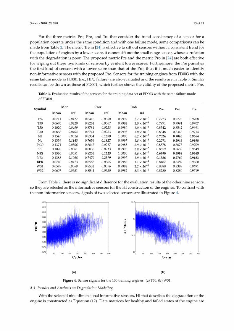
From Table 2, there is no significant difference for the evaluation results of the other nine sensors,so they are selected as the informative sensors for the HI construction of the engines. To contrast withthe non-informative sensors, signals of two selected sensors are illustrated in Figure 4.

Sensors 2020, 20, x 14 of 22

thus it is much easier to identify non-informative sensors with the proposed Pre. Sensors for the training engines from FD003 with the same failure mode as FD001 (i.e., HPC failure) are also evaluated and the results are in Table 3. Similar results can be drawn as those of FD001, which further shows the validity of the proposed metric Pre.

Table 3. Evaluation results of the sensors for the training data set of FD003 with the same failure mode of FD001.

Symbol Mon Corr Rob

Pre Pro Tre Mean std Mean std Mean std

T24 0.0711 0.0427 0.8415 0.0350 0.9997 2.7 × 10−5 0.7723 0.7723 0.9708 T30 0.0670 0.0420 0.8261 0.0367 0.9982 1.0 × 10−4 0.7991 0.7991 0.9707 T50 0.1020 0.0499 0.8781 0.0253 0.9980 1.0 × 10−4 0.8542 0.8542 0.9691 P30 0.0868 0.0404 0.8741 0.0283 0.9995 3.0 × 10−5 0.8348 0.8348 0.9714 Nf 0.1545 0.0514 0.8334 0.1098 1.0000 6.2 × 10−7 0.7024 0.7040 0.9664 Nc 0.1339 0.1143 0.7656 0.1827 0.9997 1.8 × 10−5 0.2071 0.2946 0.9198

Ps30 0.1371 0.0506 0.8847 0.0217 0.9985 8.9 × 10−5 0.8878 0.8878 0.9709 phi 0.1020 0.0501 0.8838 0.0213 0.9996 2.8 × 10−5 0.8659 0.8659 0.9649 NRf 0.1530 0.0551 0.8256 0.1225 1.0000 6.6 × 10−7 0.6990 0.6998 0.9665 NRc 0.1388 0.1098 0.7479 0.2379 0.9997 1.9 × 10−5 0.1386 0.2760 0.9183 BPR 0.0740 0.0473 0.8583 0.0305 0.9983 1.1 × 10−4 0.8487 0.8489 0.9660 W31 0.0549 0.0368 0.8532 0.0376 0.9982 1.2 × 10−4 0.8388 0.8388 0.9691 W32 0.0607 0.0351 0.8544 0.0330 0.9982 8.3 × 10−5 0.8280 0.8280 0.9719

From Table 2, there is no significant difference for the evaluation results of the other nine sensors, so they are selected as the informative sensors for the HI construction of the engines. To contrast with the non-informative sensors, signals of two selected sensors are illustrated in Figure 4.

0 50 100 150 200 250 300 350 4001570

1575

1580

1585

1590

1595

1600

1605

1610

1615

1620

0 50 100 150 200 250 300 350 40038

38.5

39

39.5

(a) (b)

Figure 4. Sensor signals for the 100 training engines: (a) T30; (b) W31.

4.3. Results and Analysis on Degradation Modeling

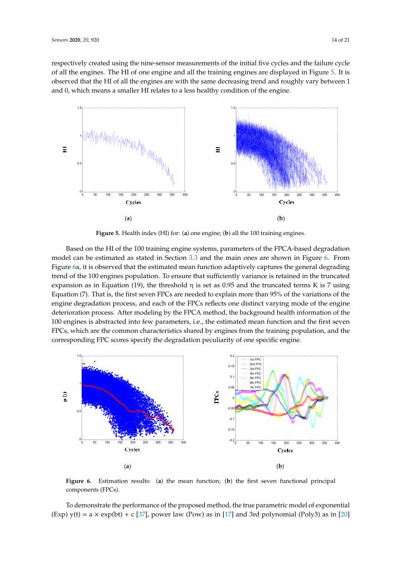
With the selected nine-dimensional informative sensors, HI that describes the degradation of the engine is constructed as Equation (12). Data matrices for healthy and failed states of the engine are respectively created using the nine-sensor measurements of the initial five cycles and the failure cycle of all the engines. The HI of one engine and all the training engines are displayed in Figure 5. It is observed that the HI of all the engines are with the same decreasing trend and roughly vary between 1 and 0, which means a smaller HI relates to a less healthy condition of the engine.

Figure 4. Sensor signals for the 100 training engines: (a) T30; (b) W31.

4.3. Results and Analysis on Degradation Modeling

With the selected nine-dimensional informative sensors, HI that describes the degradation of theengine is constructed as Equation (12). Data matrices for healthy and failed states of the engine are

Sensors 2020, 20, 920 14 of 21

respectively created using the nine-sensor measurements of the initial five cycles and the failure cycleof all the engines. The HI of one engine and all the training engines are displayed in Figure 5. It isobserved that the HI of all the engines are with the same decreasing trend and roughly vary between 1and 0, which means a smaller HI relates to a less healthy condition of the engine.

Sensors 2020, 20, x 15 of 22

0 50 100 150 200 250 300 350 4000

0.5

1

1.5

0 50 100 150 200 250 300 350 4000

0.5

1

1.5

(a) (b)

Figure 5. Health index (HI) for: (a) one engine; (b) all the 100 training engines.

Based on the HI of the 100 training engine systems, parameters of the FPCA-based degradation model can be estimated as stated in Section 3.3 and the main ones are shown in Figure 6. From Figure 6a, it is observed that the estimated mean function adaptively captures the general degrading trend of the 100 engines population. To ensure that sufficiently variance is retained in the truncated expansion as in Equation (19), the threshold η is set as 0.95 and the truncated terms K is 7 using Equation (7). That is, the first seven FPCs are needed to explain more than 95% of the variations of the engine degradation process, and each of the FPCs reflects one distinct varying mode of the engine deterioration process. After modeling by the FPCA method, the background health information of the 100 engines is abstracted into few parameters, i.e., the estimated mean function and the first seven FPCs, which are the common characteristics shared by engines from the training population, and the corresponding FPC scores specify the degradation peculiarity of one specific engine.

0 50 100 150 200 250 300 350 4000

0.5

1

1.5

0 50 100 150 200 250 300 350 400-0.2

-0.15

-0.1

-0.05

0

0.05

0.1

0.15

0.2

1st FPC2nd FPC3rd FPC4th FPC5th FPC6th FPC7th FPC

(a) (b)

Figure 6. Estimation results: (a) the mean function; (b) the first seven functional principal components (FPCs).

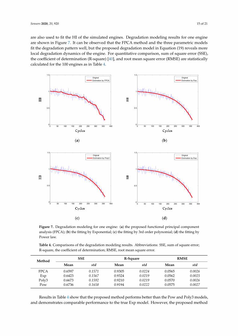
To demonstrate the performance of the proposed method, the true parametric model of exponential (Exp) y(t) = a × exp(bt) + c [37], power law (Pow) as in [17] and 3rd polynomial (Poly3) as in [20] are also used to fit the HI of the simulated engines. Degradation modeling results for one engine are shown in Figure 7. It can be observed that the FPCA method and the three parametric models fit the degradation pattern well, but the proposed degradation model

Figure 5. Health index (HI) for: (a) one engine; (b) all the 100 training engines.

Based on the HI of the 100 training engine systems, parameters of the FPCA-based degradationmodel can be estimated as stated in Section 3.3 and the main ones are shown in Figure 6. FromFigure 6a, it is observed that the estimated mean function adaptively captures the general degradingtrend of the 100 engines population. To ensure that sufficiently variance is retained in the truncatedexpansion as in Equation (19), the threshold η is set as 0.95 and the truncated terms K is 7 usingEquation (7). That is, the first seven FPCs are needed to explain more than 95% of the variations of theengine degradation process, and each of the FPCs reflects one distinct varying mode of the enginedeterioration process. After modeling by the FPCA method, the background health information of the100 engines is abstracted into few parameters, i.e., the estimated mean function and the first sevenFPCs, which are the common characteristics shared by engines from the training population, and thecorresponding FPC scores specify the degradation peculiarity of one specific engine.

Sensors 2020, 20, x 15 of 22

0 50 100 150 200 250 300 350 4000

0.5

1

1.5

0 50 100 150 200 250 300 350 4000

0.5

1

1.5

(a) (b)

Figure 5. Health index (HI) for: (a) one engine; (b) all the 100 training engines.

Based on the HI of the 100 training engine systems, parameters of the FPCA-based degradation model can be estimated as stated in Section 3.3 and the main ones are shown in Figure 6. From Figure 6a, it is observed that the estimated mean function adaptively captures the general degrading trend of the 100 engines population. To ensure that sufficiently variance is retained in the truncated expansion as in Equation (19), the threshold η is set as 0.95 and the truncated terms K is 7 using Equation (7). That is, the first seven FPCs are needed to explain more than 95% of the variations of the engine degradation process, and each of the FPCs reflects one distinct varying mode of the engine deterioration process. After modeling by the FPCA method, the background health information of the 100 engines is abstracted into few parameters, i.e., the estimated mean function and the first seven FPCs, which are the common characteristics shared by engines from the training population, and the corresponding FPC scores specify the degradation peculiarity of one specific engine.

0 50 100 150 200 250 300 350 4000

0.5

1

1.5

0 50 100 150 200 250 300 350 400-0.2

-0.15

-0.1

-0.05

0

0.05

0.1

0.15

0.2

1st FPC2nd FPC3rd FPC4th FPC5th FPC6th FPC7th FPC

(a) (b)

Figure 6. Estimation results: (a) the mean function; (b) the first seven functional principal components (FPCs).

To demonstrate the performance of the proposed method, the true parametric model of exponential (Exp) y(t) = a × exp(bt) + c [37], power law (Pow) as in [17] and 3rd polynomial (Poly3) as in [20] are also used to fit the HI of the simulated engines. Degradation modeling results for one engine are shown in Figure 7. It can be observed that the FPCA method and the three parametric models fit the degradation pattern well, but the proposed degradation model

Figure 6. Estimation results: (a) the mean function; (b) the first seven functional principalcomponents (FPCs).

To demonstrate the performance of the proposed method, the true parametric model of exponential(Exp) y(t) = a × exp(bt) + c [37], power law (Pow) as in [17] and 3rd polynomial (Poly3) as in [20]

Sensors 2020, 20, 920 15 of 21

are also used to fit the HI of the simulated engines. Degradation modeling results for one engineare shown in Figure 7. It can be observed that the FPCA method and the three parametric modelsfit the degradation pattern well, but the proposed degradation model in Equation (19) reveals morelocal degradation dynamics of the engine. For quantitative comparison, sum of square error (SSE),the coefficient of determination (R-square) [40], and root mean square error (RMSE) are statisticallycalculated for the 100 engines as in Table 4.

Sensors 2020, 20, x 16 of 22

in Equation (19) reveals more local degradation dynamics of the engine. For quantitative comparison, sum of square error (SSE), the coefficient of determination (R-square) [40], and root mean square error (RMSE) are statistically calculated for the 100 engines as in Table 4.

0 50 100 150 200 250 300 350 4000

0.5

1

1.5

OriginalEstimation by FPCA

0 50 100 150 200 250 300 350 4000

0.5

1

1.5

OriginalEstimation by Exp

(a) (b)

0 50 100 150 200 250 300 350 4000

0.5

1

1.5

OriginalEstimation by Poly3

0 50 100 150 200 250 300 350 4000

0.5

1

1.5

OriginalEstimation by Exp

(c) (d)

Figure 7. Degradation modeling for one engine: (a) the proposed functional principal component analysis (FPCA); (b) the fitting by Exponential; (c) the fitting by 3rd order polynomial; (d) the fitting by Power law.

Table 4. Comparisons of the degradation modeling results. Abbreviations: SSE, sum of square error; R-square, the coefficient of determination; RMSE, root mean square error.

Method SSE R-Square RMSE Mean std Mean std Mean std

FPCA 0.6597 0.1571 0.9305 0.0224 0.0565 0.0026 Exp 0.6423 0.1567 0.9324 0.0219 0.0562 0.0025

Poly3 0.6673 0.1592 0.9210 0.0219 0.0570 0.0026 Pow 0.6736 0.1658 0.9194 0.0222 0.0575 0.0027

Results in Table 4 show that the proposed method performs better than the Pow and Poly3 models, and demonstrates comparable performance to the true Exp model. However, the proposed method models the degradation adaptively without any assumption on the parametric form of the degradation pattern. This will be more significant when little knowledge is known about the latent degradation trend. Also, all the 100 engine degradation observations from the training set are pooled to estimate the parameters of the proposed degradation model. While in the parametric models, fittings are carried out with one individual engine

Figure 7. Degradation modeling for one engine: (a) the proposed functional principal componentanalysis (FPCA); (b) the fitting by Exponential; (c) the fitting by 3rd order polynomial; (d) the fitting byPower law.

Table 4. Comparisons of the degradation modeling results. Abbreviations: SSE, sum of square error;R-square, the coefficient of determination; RMSE, root mean square error.

MethodSSE R-Square RMSE

Mean std Mean std Mean std

FPCA 0.6597 0.1571 0.9305 0.0224 0.0565 0.0026Exp 0.6423 0.1567 0.9324 0.0219 0.0562 0.0025

Poly3 0.6673 0.1592 0.9210 0.0219 0.0570 0.0026Pow 0.6736 0.1658 0.9194 0.0222 0.0575 0.0027

Results in Table 4 show that the proposed method performs better than the Pow and Poly3 models,and demonstrates comparable performance to the true Exp model. However, the proposed method

Sensors 2020, 20, 920 16 of 21

models the degradation adaptively without any assumption on the parametric form of the degradationpattern. This will be more significant when little knowledge is known about the latent degradationtrend. Also, all the 100 engine degradation observations from the training set are pooled to estimate theparameters of the proposed degradation model. While in the parametric models, fittings are carriedout with one individual engine independently, common information about the degradation processof the engine population is prone to be lost. In the following, the FPCA method is combined withBayesian inference to predict the aero-engine health and comparison are made with the true Expdegadation model.

4.4. Results and Analysis on Health Prognostics

For validation of the presented method for long-term health prognostics, the multiple sensordata of the 100 testing engines from FD001 is processed following the same procedures of the trainingengines as detailed above.

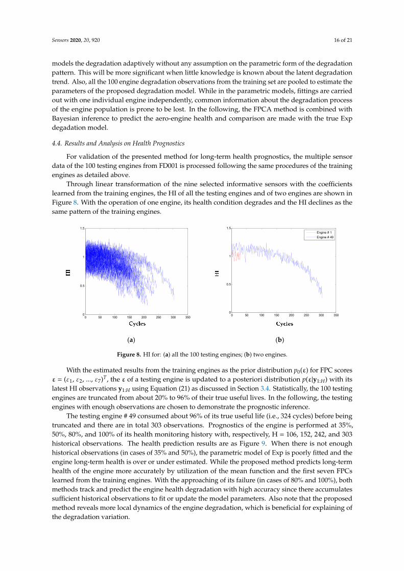
Through linear transformation of the nine selected informative sensors with the coefficientslearned from the training engines, the HI of all the testing engines and of two engines are shown inFigure 8. With the operation of one engine, its health condition degrades and the HI declines as thesame pattern of the training engines.

Sensors 2020, 20, x 17 of 22

independently, common information about the degradation process of the engine population is prone to be lost. In the following, the FPCA method is combined with Bayesian inference to predict the aero-engine health and comparison are made with the true Exp degadation model.

4.4. Results and Analysis on Health Prognostics

For validation of the presented method for long-term health prognostics, the multiple sensor data of the 100 testing engines from FD001 is processed following the same procedures of the training engines as detailed above.

Through linear transformation of the nine selected informative sensors with the coefficients learned from the training engines, the HI of all the testing engines and of two engines are shown in Figure 8. With the operation of one engine, its health condition degrades and the HI declines as the same pattern of the training engines.

0 50 100 150 200 250 300 3500

0.5

1

1.5

0 50 100 150 200 250 300 3500

0.5

1

1.5

Engine # 1Engine # 49

(a) (b)

Figure 8. HI for: (a) all the 100 testing engines; (b) two engines.

With the estimated results from the training engines as the prior distribution p0(ε) for FPC scores ε = (ε1, ε2, ..., ε7)T, the ε of a testing engine is updated to a posteriori distribution p(ε|y1:H) with its latest HI observations y1:H using Equation (21) as discussed in SubSection 3.4. Statistically, the 100 testing engines are truncated from about 20% to 96% of their true useful lives. In the following, the testing engines with enough observations are chosen to demonstrate the prognostic inference.

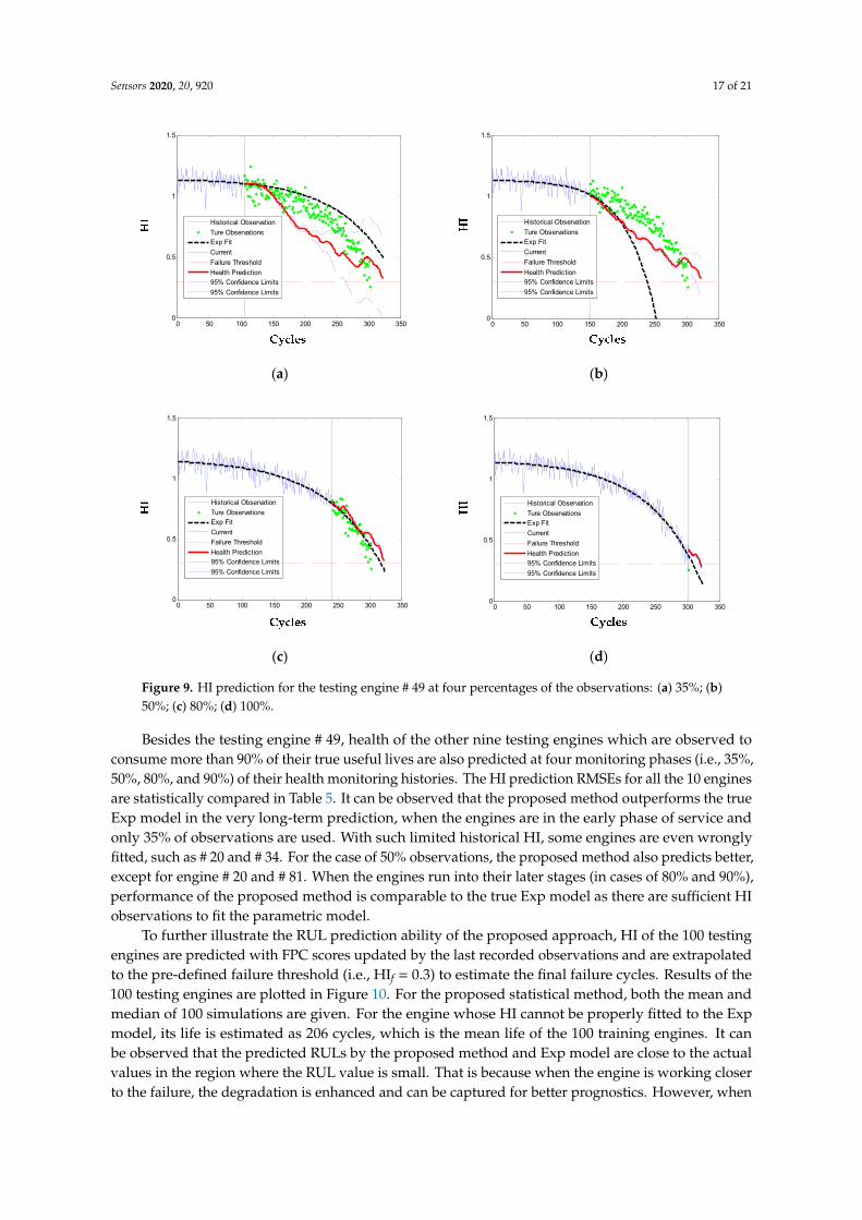
The testing engine # 49 consumed about 96% of its true useful life (i.e., 324 cycles) before being truncated and there are in total 303 observations. Prognostics of the engine is performed at 35%, 50%, 80%, and 100% of its health monitoring history with, respectively, H = 106, 152, 242, and 303 historical observations. The health prediction results are as Figure 9. When there is not enough historical observations (in cases of 35% and 50%), the parametric model of Exp is poorly fitted and the engine long-term health is over or under estimated. While the proposed method predicts long-term health of the engine more accurately by utilization of the mean function and the first seven FPCs learned from the training engines. With the approaching of its failure (in cases of 80% and 100%), both methods track and predict the engine health degradation with high accuracy since there accumulates sufficient historical observations to fit or update the model parameters. Also note that the proposed method reveals more local dynamics of the engine degradation, which is beneficial for explaining of the degradation variation.

Figure 8. HI for: (a) all the 100 testing engines; (b) two engines.

With the estimated results from the training engines as the prior distribution p0(ε) for FPC scoresε = (ε1, ε2, ..., ε7)T, the ε of a testing engine is updated to a posteriori distribution p(ε|y1:H) with itslatest HI observations y1:H using Equation (21) as discussed in Section 3.4. Statistically, the 100 testingengines are truncated from about 20% to 96% of their true useful lives. In the following, the testingengines with enough observations are chosen to demonstrate the prognostic inference.

The testing engine # 49 consumed about 96% of its true useful life (i.e., 324 cycles) before beingtruncated and there are in total 303 observations. Prognostics of the engine is performed at 35%,50%, 80%, and 100% of its health monitoring history with, respectively, H = 106, 152, 242, and 303historical observations. The health prediction results are as Figure 9. When there is not enoughhistorical observations (in cases of 35% and 50%), the parametric model of Exp is poorly fitted and theengine long-term health is over or under estimated. While the proposed method predicts long-termhealth of the engine more accurately by utilization of the mean function and the first seven FPCslearned from the training engines. With the approaching of its failure (in cases of 80% and 100%), bothmethods track and predict the engine health degradation with high accuracy since there accumulatessufficient historical observations to fit or update the model parameters. Also note that the proposedmethod reveals more local dynamics of the engine degradation, which is beneficial for explaining ofthe degradation variation.

Sensors 2020, 20, 920 17 of 21Sensors 2020, 20, x 18 of 22

0 50 100 150 200 250 300 3500

0.5

1

1.5

Historical ObservationTure ObservationsExp FitCurrentFailure ThresholdHealth Prediction95% Confidence Limits95% Confidence Limits

0 50 100 150 200 250 300 3500

0.5

1

1.5

Historical ObservationTure ObservationsExp FitCurrentFailure ThresholdHealth Prediction95% Confidence Limits95% Confidence Limits

(a) (b)

0 50 100 150 200 250 300 3500

0.5

1

1.5

Historical ObservationTure ObservationsExp FitCurrentFailure ThresholdHealth Prediction95% Confidence Limits95% Confidence Limits

0 50 100 150 200 250 300 3500

0.5

1

1.5

Historical ObservationTure ObservationsExp FitCurrentFailure ThresholdHealth Prediction95% Confidence Limits95% Confidence Limits

(c) (d)

Figure 9. HI prediction for the testing engine # 49 at four percentages of the observations: (a) 35%; (b) 50%; (c) 80%; (d) 100%.

Besides the testing engine # 49, health of the other nine testing engines which are observed to consume more than 90% of their true useful lives are also predicted at four monitoring phases (i.e., 35%, 50%, 80%, and 90%) of their health monitoring histories. The HI prediction RMSEs for all the 10 engines are statistically compared in Table 5. It can be observed that the proposed method outperforms the true Exp model in the very long-term prediction, when the engines are in the early phase of service and only 35% of observations are used. With such limited historical HI, some engines are even wrongly fitted, such as # 20 and # 34. For the case of 50% observations, the proposed method also predicts better, except for engine # 20 and # 81. When the engines run into their later stages (in cases of 80% and 90%), performance of the proposed method is comparable to the true Exp model as there are sufficient HI observations to fit the parametric model.

Figure 9. HI prediction for the testing engine # 49 at four percentages of the observations: (a) 35%; (b)50%; (c) 80%; (d) 100%.

Besides the testing engine # 49, health of the other nine testing engines which are observed toconsume more than 90% of their true useful lives are also predicted at four monitoring phases (i.e., 35%,50%, 80%, and 90%) of their health monitoring histories. The HI prediction RMSEs for all the 10 enginesare statistically compared in Table 5. It can be observed that the proposed method outperforms the trueExp model in the very long-term prediction, when the engines are in the early phase of service andonly 35% of observations are used. With such limited historical HI, some engines are even wronglyfitted, such as # 20 and # 34. For the case of 50% observations, the proposed method also predicts better,except for engine # 20 and # 81. When the engines run into their later stages (in cases of 80% and 90%),performance of the proposed method is comparable to the true Exp model as there are sufficient HIobservations to fit the parametric model.

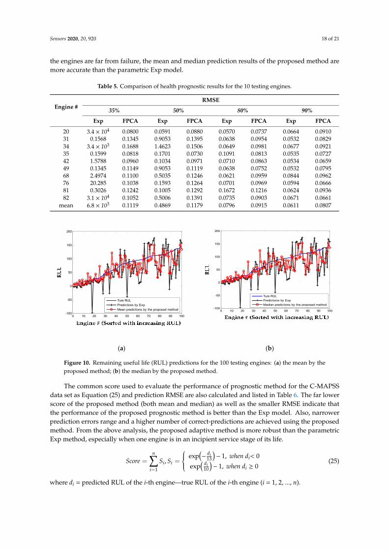
To further illustrate the RUL prediction ability of the proposed approach, HI of the 100 testingengines are predicted with FPC scores updated by the last recorded observations and are extrapolatedto the pre-defined failure threshold (i.e., HIf = 0.3) to estimate the final failure cycles. Results of the100 testing engines are plotted in Figure 10. For the proposed statistical method, both the mean andmedian of 100 simulations are given. For the engine whose HI cannot be properly fitted to the Expmodel, its life is estimated as 206 cycles, which is the mean life of the 100 training engines. It canbe observed that the predicted RULs by the proposed method and Exp model are close to the actualvalues in the region where the RUL value is small. That is because when the engine is working closerto the failure, the degradation is enhanced and can be captured for better prognostics. However, when

Sensors 2020, 20, 920 18 of 21

the engines are far from failure, the mean and median prediction results of the proposed method aremore accurate than the parametric Exp model.

Table 5. Comparison of health prognostic results for the 10 testing engines.

Engine #RMSE

35% 50% 80% 90%

Exp FPCA Exp FPCA Exp FPCA Exp FPCA

20 3.4 × 104 0.0800 0.0591 0.0880 0.0570 0.0737 0.0664 0.091031 0.1568 0.1345 0.9053 0.1395 0.0638 0.0954 0.0532 0.082934 3.4 × 103 0.1688 1.4623 0.1506 0.0649 0.0981 0.0677 0.092135 0.1599 0.0818 0.1701 0.0730 0.1091 0.0813 0.0535 0.072742 1.5788 0.0960 0.1034 0.0971 0.0710 0.0863 0.0534 0.065949 0.1345 0.1149 0.9053 0.1119 0.0638 0.0752 0.0532 0.079568 2.4974 0.1100 0.5035 0.1246 0.0621 0.0959 0.0844 0.096276 20.285 0.1038 0.1593 0.1264 0.0701 0.0969 0.0594 0.066681 0.3026 0.1242 0.1005 0.1292 0.1672 0.1216 0.0624 0.093682 3.1 × 104 0.1052 0.5006 0.1391 0.0735 0.0903 0.0671 0.0661

mean 6.8 × 103 0.1119 0.4869 0.1179 0.0796 0.0915 0.0611 0.0807

Sensors 2020, 20, x 19 of 22

Table 5. Comparison of health prognostic results for the 10 testing engines.

Engine # RMSE

35% 50% 80% 90% Exp FPCA Exp FPCA Exp FPCA Exp FPCA

20 3.4 × 104 0.0800 0.0591 0.0880 0.0570 0.0737 0.0664 0.0910 31 0.1568 0.1345 0.9053 0.1395 0.0638 0.0954 0.0532 0.0829 34 3.4 × 103 0.1688 1.4623 0.1506 0.0649 0.0981 0.0677 0.0921 35 0.1599 0.0818 0.1701 0.0730 0.1091 0.0813 0.0535 0.0727 42 1.5788 0.0960 0.1034 0.0971 0.0710 0.0863 0.0534 0.0659 49 0.1345 0.1149 0.9053 0.1119 0.0638 0.0752 0.0532 0.0795 68 2.4974 0.1100 0.5035 0.1246 0.0621 0.0959 0.0844 0.0962 76 20.285 0.1038 0.1593 0.1264 0.0701 0.0969 0.0594 0.0666 81 0.3026 0.1242 0.1005 0.1292 0.1672 0.1216 0.0624 0.0936 82 3.1 × 104 0.1052 0.5006 0.1391 0.0735 0.0903 0.0671 0.0661

mean 6.8 × 103 0.1119 0.4869 0.1179 0.0796 0.0915 0.0611 0.0807

To further illustrate the RUL prediction ability of the proposed approach, HI of the 100 testing engines are predicted with FPC scores updated by the last recorded observations and are extrapolated to the pre-defined failure threshold (i.e., HIf = 0.3) to estimate the final failure cycles. Results of the 100 testing engines are plotted in Figure 10. For the proposed statistical method, both the mean and median of 100 simulations are given. For the engine whose HI cannot be properly fitted to the Exp model, its life is estimated as 206 cycles, which is the mean life of the 100 training engines. It can be observed that the predicted RULs by the proposed method and Exp model are close to the actual values in the region where the RUL value is small. That is because when the engine is working closer to the failure, the degradation is enhanced and can be captured for better prognostics. However, when the engines are far from failure, the mean and median prediction results of the proposed method are more accurate than the parametric Exp model.

0 10 20 30 40 50 60 70 80 90 100-100

-50

0

50

100

150

200

Ture RULPredictions by ExpMean predictions by the proposed method

0 10 20 30 40 50 60 70 80 90 100-100

-50

0

50

100

150

200

Ture RULPredictions by ExpMedian predictions by the proposed method

(a) (b)

Figure 10. Remaining useful life (RUL) predictions for the 100 testing engines: (a) the mean by the proposed method; (b) the median by the proposed method.

The common score used to evaluate the performance of prognostic method for the C-MAPSS data set as Equation (25) and prediction RMSE are also calculated and listed in Table 6. The far lower score of the proposed method (both mean and median) as well as the smaller RMSE indicate that the performance of the proposed prognostic method is better than the Exp

Figure 10. Remaining useful life (RUL) predictions for the 100 testing engines: (a) the mean by theproposed method; (b) the median by the proposed method.

The common score used to evaluate the performance of prognostic method for the C-MAPSSdata set as Equation (25) and prediction RMSE are also calculated and listed in Table 6. The far lowerscore of the proposed method (both mean and median) as well as the smaller RMSE indicate thatthe performance of the proposed prognostic method is better than the Exp model. Also, narrowerprediction errors range and a higher number of correct-predictions are achieved using the proposedmethod. From the above analysis, the proposed adaptive method is more robust than the parametricExp method, especially when one engine is in an incipient service stage of its life.

Score =n∑

i=1

Si, Si =

exp(−

di13

)− 1, when di< 0

exp( di

10

)− 1, when di ≥ 0

(25)

where di = predicted RUL of the i-th engine—true RUL of the i-th engine (i = 1, 2, ..., n).

Sensors 2020, 20, 920 19 of 21

Table 6. Comparison of RUL prediction results for the 100 testing engines.

Method Score RMSE Rang of PredictionErrors

Under-Predictions

Correct-Predictions

Over-Predictions

Exp 67,352 45.40 [−135, 63] 76 1 23

FPCAmean 3092 28.06 [−82, 65] 65 3 32

median 3567 28.70 [−83, 68] 67 5 28

5. Discussion

In this paper, a data-driven statistical prognostic approach for informative sensor selection andadaptive degradation modeling based on FPCA is introduced. Effectiveness of the proposed methodis validated by the case study on an aircraft engine simulation experiment. Nevertheless, some keyissues should be tackled for application of the presented method to real engines and other systems.

For the proposed approach to be effective for real engines, enough run-to-failure sensor datashould be provided, and this is a common requirement for a data-driven approach. In real aircraftengine operation, the degradation of one engine usually begins after one long normal working stage,the so-called delay-time phenomenon. Modeling of the potential-to-failure stage is of more significance.Thus, it is better to apply the proposed method upon the detection of incipient faults. For few instancesof real engine failures, and that is often the case, the jointly Gaussian assumption may no longer holdfor the parameter estimation. To partially tackle this problem, some kind of bootstrap methods can beuseful. As for the extension of the proposed method, especially the adaptive degradation modeling byFPCA, to monitor other systems, efforts should be put especially to the construction of a HI that relatesto the degradation of these systems, as the linear data transformation method used in this paper maynot be applicable.

6. Conclusions

To model and track the complex degradation pattern of aircraft engines for accurate and efficientprognosis, a novel method for informative sensor selection and adaptive degradation track is proposedin this paper. The deterioration sensitive sensors can be selected by the presented metrics and be fusedto construct a health index that describes the degradation of an aircraft engine. Taking the degradationindex of one engine as functional data, the degradation process of the engine population is thenadaptively modeled by the FPCA, and future health is predicted with Bayesian inference. Experimentalstudies are performed on the sensor dataset of aircraft gas turbine engines, and the results verify thatthe proposed method can effectively select the informative sensors to model and predict the complexdegradation process of the aircraft engine. The failure threshold is set to a fixed value in this study;however, large variation of the failure value requires a random failure threshold to be pursued inthe future.

Author Contributions: Conceptualization, B.Z. and Q.H.; methodology, B.Z.; software, B.Z.; validation,B.Z., Q.H., and K.Z.; formal analysis, S.F.; investigation, B.Z. and S.Z.; resources, B.Z.; data curation, B.Z.;writing—original draft preparation, B.Z.; writing—review and editing, B.Z.; visualization, Y.Z.; supervision, Y.Z.;project administration, B.Z.; funding acquisition, Q.H. and B.Z. All authors have read and agreed to the publishedversion of the manuscript.

Funding: This research was funded by the National Natural Science Foundation of China (NSFC) (Grant No.51605065 & No. 51905065), the Science and Technology Research Program of Chongqing Municipal EducationCommission (Grant No. KJ1704109), and the Open Found of The State Key Laboratory of Mechanical Transmissions(Grant No. SKLMT-KFKT-201809).

Conflicts of Interest: The authors declare no conflicts of interest.

References

1. Volponi, A.J. Gas turbine engine health management: Past, present, and future trends. J. Eng. GasTurbines Power 2014, 136, 051201. [CrossRef]

Sensors 2020, 20, 920 20 of 21

2. Lei, Y.G.; Li, N.P.; Guo, L.; Li, N.B.; Yao, T.; Lin, J. Machinery health prognostics: A systematic review fromdata acquisition to RUL prediction. Mech. Syst. Signal Process. 2018, 104, 799–834. [CrossRef]

3. Hanachi, H.; Mechefske, C.; Liu, J.; Banerjee, A.; Chen, Y. Performance-based gas turbine health monitoring,diagnostics, and prognostics: A survey. IEEE Trans. Reliab. 2018, 67, 1340–1363. [CrossRef]

4. Wang, P.; Gao, R.X. Markov nonlinear system estimation for engine performance tracking. J. Eng. GasTurbines Power 2016, 138, 091201. [CrossRef]

5. Al-Dahidi, S.; Di Maio, F.; Baraldi, P.; Zio, E. Remaining useful life estimation in heterogeneous fleets workingunder variable operating conditions. Reliab. Eng. Syst. Saf. 2016, 156, 109–124. [CrossRef]

6. Yu, J.B. Aircraft engine health prognostics based on logistic regression with penalization regularization andstate-space-based degradation framework. Aerosp. Sci. Technol. 2017, 68, 345–361. [CrossRef]

7. Skordilis, E.; Moghaddass, R. A double hybrid state-Space model for real-time sensor-driven monitoring ofdeteriorating systems. IEEE Trans. Autom. Sci. Eng. 2019. [CrossRef]

8. Mosallam, A.; Medjaher, K.; Zerhouni, N. Data-driven prognostic method based on Bayesian approaches fordirect remaining useful life prediction. J. Intell. Manuf. 2016, 27, 1037–1048. [CrossRef]

9. Wang, C.S.; Lu, N.Y.; Cheng, Y.H.; Jiang, B. A data-driven aero-engine degradation prognostic strategy.IEEE Trans. Cybern. 2019. [CrossRef]

10. Khelif, R.; Chebel-Morello, B.; Malinowski, S.; Laajili, E.; Fnaiech, F.; Zerhouni, N. Direct remaining usefullife estimation based on support vector regression. IEEE Trans. Ind. Electron. 2016, 64, 2276–2285. [CrossRef]

11. Lu, F.; Wu, J.D.; Huang, J.Q.; Qiu, X.J. Aircraft engine degradation prognostics based on logistic regressionand novel OS-ELM algorithm. Aerosp. Sci. Technol. 2019, 84, 661–671. [CrossRef]

12. Huang, C.G.; Huang, H.Z.; Li, Y.F. A Bi-Directional LSTM prognostics method under multiple operationalconditions. IEEE Trans. Ind. Electron. 2019, 66, 8792–8802. [CrossRef]

13. Li, Z.X.; Goebel, K.; Wu, D.Z. Degradation modeling and remaining useful life prediction of aircraft enginesusing ensemble learning. J. Eng. Gas Turbines Power 2019, 141, 041008. [CrossRef]

14. Si, X.S.; Wang, W.; Hu, C.H.; Zhou, D.H. Remaining useful life estimation–a review on the statistical datadriven approaches. Eur. J. Oper. Res. 2011, 213, 1–14. [CrossRef]

15. Lasheras, S.F.; Nieto, P.J.G.; De Cos Juez, F.J.; Bayón, R.M.; Suárez, V.M.G. A hybrid PCA-CART-MARS-basedprognostic approach of the remaining useful life for aircraft engines. Sensors 2015, 15, 7062–7083. [CrossRef][PubMed]

16. Zaidan, M.A.; Mills, A.R.; Harrison, R.F.; Fleming, P.J. Gas turbine engine prognostics using Bayesianhierarchical models: A variational approach. Mech. Syst. Signal Process. 2016, 70–71, 120–140. [CrossRef]

17. Liu, K.B.; Huang, S. Integration of data fusion methodology and degradation modeling process to improveprognostics. IEEE Trans. Autom. Sci. Eng. 2016, 13, 344–354. [CrossRef]

18. Song, C.Y.; Liu, K.B. Statistical degradation modeling and prognostics of multiple sensor signals via datafusion: A composite health index approach. IISE Trans. 2018, 50, 853–867. [CrossRef]

19. Zhang, Z.X.; Si, X.S.; Hu, C.H.; Lei, Y.G. Degradation data analysis and remaining useful life estimation: Areview on Wiener-process-based methods. Eur. J. Oper. Res. 2018, 271, 775–796. [CrossRef]

20. Le Son, K.; Fouladirad, M.; Barros, A. Remaining useful lifetime estimation and noisy gamma deteriorationprocess. Reliab. Eng. Syst. Saf. 2016, 149, 76–87. [CrossRef]

21. Peng, W.W.; Li, Y.F.; Yang, Y.J.; Mi, J.; Huang, H.Z. Bayesian degradation analysis with inverse Gaussianprocess models under time-varying degradation rates. IEEE Trans. Reliab. 2017, 66, 84–96. [CrossRef]

22. Wang, P.F.; Youn, B.D.; Hu, C. A generic probabilistic framework for structural health prognostics anduncertainty management. Mech. Syst. Signal Process. 2012, 28, 622–637. [CrossRef]

23. Kim, M.; Song, C.; Liu, K. A generic health index approach for multisensor degradation modeling and sensorselection. IEEE Trans. Autom. Sci. Eng. 2019, 16, 1426–1437. [CrossRef]

24. Coble, J.; Hines, J.W. Applying the general path model to estimation of remaining useful life. Int. J. Progn.Health Manag. 2011, 2, 71–82.

25. Liu, L.S.; Wang, S.J.; Liu, D.T.; Peng, Y. Quantitative selection of sensor data based on improved permutationentropy for system remaining useful life prediction. Microelectron. Reliab. 2017, 75, 264–270. [CrossRef]

26. Chehade, A.; Shi, Z.Y. Sensor fusion via statistical hypothesis testing for prognosis and degradation analysis.IEEE Trans. Autom. Sci. Eng. 2019, 16, 1774–1787. [CrossRef]

27. Fang, X.L.; Paynabar, K.; Gebraeel, N. Multistream sensor fusion-based prognostics model for systems withsingle failure modes. Reliab. Eng. Syst. Saf. 2017, 159, 322–331. [CrossRef]

Sensors 2020, 20, 920 21 of 21

28. Ye, Z.S.; Xie, M. Stochastic modelling and analysis of degradation for highly reliable products. Appl. Stoch.Models Bus. Ind. 2015, 31, 16–32. [CrossRef]

29. Zhang, B.; Zhang, L.J.; Xu, J.W. Degradation feature selection for remaining useful life prediction of rollingelement bearings. Qual. Reliab. Eng. Int. 2016, 32, 547–554. [CrossRef]

30. Shang, H.L. A survey of functional principal component analysis. AStA Adv. Stat. Anal. 2014, 98, 121–142.[CrossRef]

31. Wang, J.L.; Chiou, J.; Müller, H.G. Functional data analysis. Annu. Rev. Stat. Its Appl. 2016, 3, 257–295.[CrossRef]

32. Chung, S.; Kontar, R. Functional principal component analysis for extrapolating multi-stream longitudinaldata. arXiv Preprint 2019, arXiv:1903.03871.

33. Ghahramani, Z. Bayesian non-parametrics and the probabilistic approach to modelling. Philos. Trans. R. Soc.A Math. Phys. Eng. Sci. 2013, 371, 20110553. [CrossRef] [PubMed]

34. Fang, X.L.; Zhou, R.R.; Gebraeel, N. An adaptive functional regression-based prognostic model for applicationswith missing data. Reliab. Eng. Syst. Saf. 2015, 133, 266–274. [CrossRef]

35. Yao, F.; Müller, H.G.; Wang, J.L. Functional data analysis for sparse longitudinal data. J. Am. Stat. Assoc.2005, 100, 577–590. [CrossRef]

36. Zhou, R.R.; Serban, N.; Gebraeel, N. Degradation applied to residual lifetime prediction using functionaldata analysis. Ann. Appl. Stat. 2011, 5, 1586–1610. [CrossRef]

37. Saxena, A.; Goebel, K.; Simon, D.; Eklund, N. Damage Propagation for Aircraft Engine Run-To-FailureSimulation. In Proceedings of the International Conference on Prognostics and Health Management, Denver,CO, USA, 6–9 October 2008.

38. Saxena, A.; Goebel, K. Turbo Fan Engine Degradation Simulation Dataset. In NASA Ames Prognostics DataRepository; NASA Ames: Moffett Field, CA, USA, 2012. Available online: http://ti.arc.nasa.gov/tech/dash/

pcoe/prognostic-data-repository (accessed on 15 August 2018).39. Singh, S.K.; Kumar, S.; Dwivedi, J.P. A novel soft computing method for engine RUL prediction.

Multimed. Tools Appl. 2019, 78, 4065–4087. [CrossRef]40. Nieto, P.J.G.; García-Gonzalo, E.; Lasheras, S.F.; De Cos Juez, F.J. Hybrid PSO–SVM-based method for

forecasting of the remaining useful life for aircraft engines and evaluation of its reliability. Reliab. Eng.Syst. Saf. 2015, 138, 219–231. [CrossRef]

© 2020 by the authors. Licensee MDPI, Basel, Switzerland. This article is an open accessarticle distributed under the terms and conditions of the Creative Commons Attribution(CC BY) license (http://creativecommons.org/licenses/by/4.0/).