AirPhoto SEVersion 2.67

Reference Manual23 June 2017

Table of ContentsOverview..............................................................................................................................................3Oblique Image Correction....................................................................................................................5File Input & Output..............................................................................................................................8Toolbars and Menus............................................................................................................................13Control Points.....................................................................................................................................17Image Treatment.................................................................................................................................26Transformation...................................................................................................................................28Transformation with an arbitrary grid................................................................................................33Transformation of images with known proportions...........................................................................41Transformation with Total Station Coordinates..................................................................................44Printing...............................................................................................................................................54Options...............................................................................................................................................55GeoPortal Data...................................................................................................................................59Editing Control or Calibration Points.................................................................................................85Calibrating GeoPortal Variants...........................................................................................................89Special Capture Window....................................................................................................................95EPSG Grids......................................................................................................................................101Google Earth Pro Installation...........................................................................................................106Google Earth Pro Started from AirPhotoSE.....................................................................................108Google Earth.....................................................................................................................................128Google Earth Find a place name with Google Maps........................................................................138Calibrating Google Earth Images.....................................................................................................139Trigonometric and Navigation Aid Points........................................................................................147Google Earth: Improving Accuracy..................................................................................................153Google Earth: Combining multiple year captures............................................................................164Distance, perimeter and area measurement......................................................................................171Orthophotos from multiple images...................................................................................................174Using CloudCompare + ICE for many images.................................................................................194Orthophoto Preview..........................................................................................................................199Orthophoto Options..........................................................................................................................207Scanned Film Verticals, Cropping Black Borders............................................................................210Layers...............................................................................................................................................218Local Stretch.....................................................................................................................................228Local Stretch Theory........................................................................................................................236Acknowledgements..........................................................................................................................239Technical Notes................................................................................................................................240Bibliography.....................................................................................................................................245Installation Notes..............................................................................................................................247New and changed features:...............................................................................................................255

2

Overview

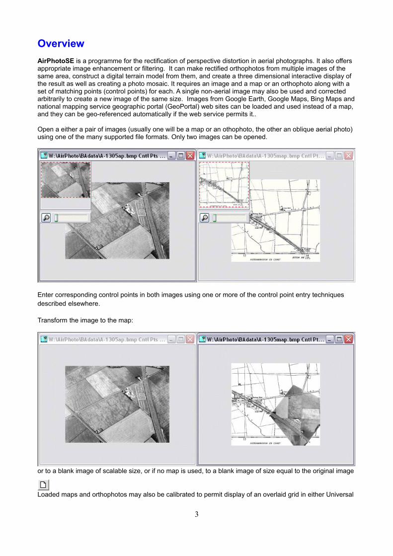
AirPhotoSE is a programme for the rectification of perspective distortion in aerial photographs. It also offers appropriate image enhancement or filtering. It can make rectified orthophotos from multiple images of the same area, construct a digital terrain model from them, and create a three dimensional interactive display of the result as well as creating a photo mosaic. It requires an image and a map or an orthophoto along with a set of matching points (control points) for each. A single non-aerial image may also be used and corrected arbitrarily to create a new image of the same size. Images from Google Earth, Google Maps, Bing Maps andnational mapping service geographic portal (GeoPortal) web sites can be loaded and used instead of a map, and they can be geo-referenced automatically if the web service permits it..

Open a either a pair of images (usually one will be a map or an othophoto, the other an oblique aerial photo) using one of the many supported file formats. Only two images can be opened.

Enter corresponding control points in both images using one or more of the control point entry techniques described elsewhere.

Transform the image to the map:

or to a blank image of scalable size, or if no map is used, to a blank image of size equal to the original image

Loaded maps and orthophotos may also be calibrated to permit display of an overlaid grid in either Universal

3

Transverse Mercator (UTM), decimal Latitude/Longitude, or arbitrary X-Y coordinates. Optionally, a national or international grids from the European Petroleum Survey Group database may be chosen. The coordinatesin the chosen grid at the position of the mouse cursor are displayed continuously. Otherwise, the position of the cursor in pixels is shown. Optionally, they are also recorded in files suitable for use with a common geographic information system.

Save the result to a new file for use in other programmes. Print the result if desired.

4

Oblique Image Correction

Displaying images:

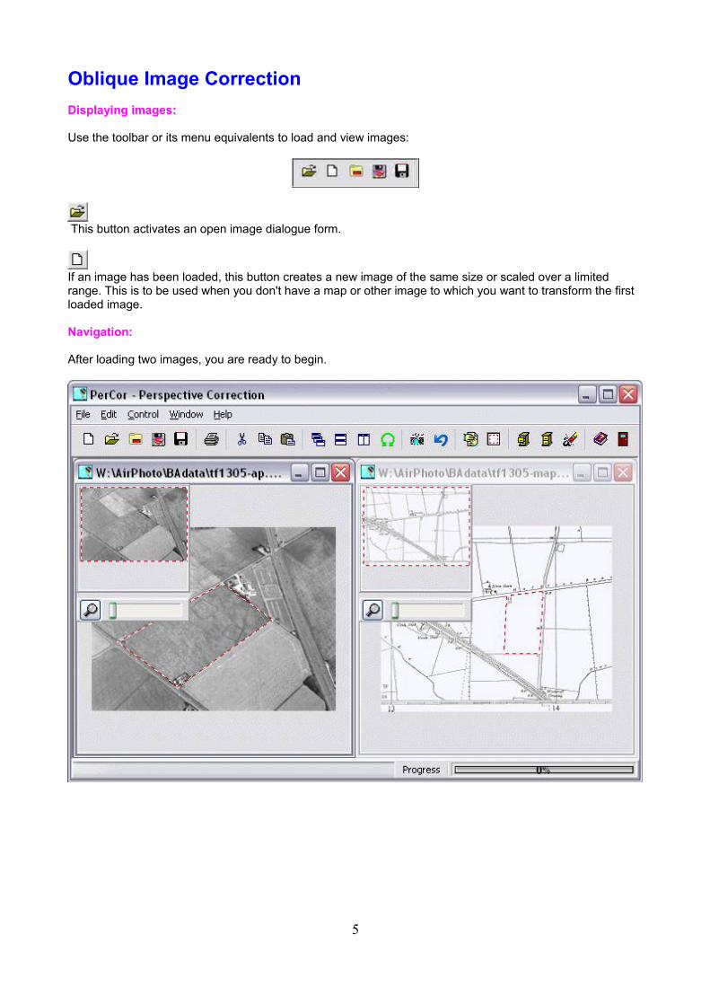
Use the toolbar or its menu equivalents to load and view images:

This button activates an open image dialogue form.

If an image has been loaded, this button creates a new image of the same size or scaled over a limited range. This is to be used when you don't have a map or other image to which you want to transform the first loaded image.

Navigation:

After loading two images, you are ready to begin.

5

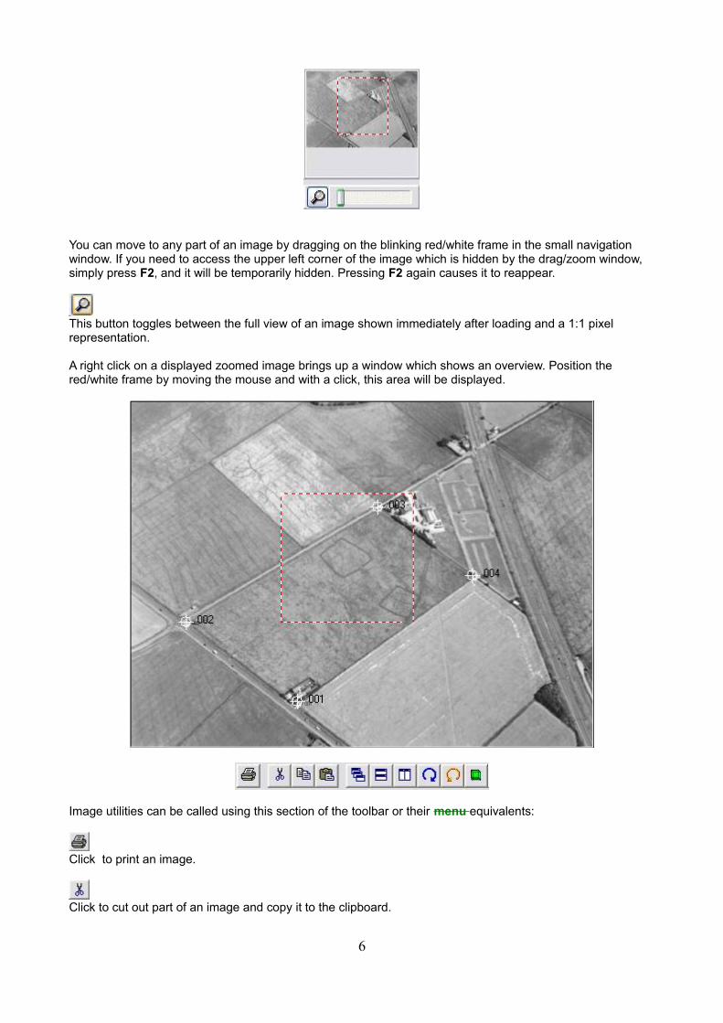
You can move to any part of an image by dragging on the blinking red/white frame in the small navigation window. If you need to access the upper left corner of the image which is hidden by the drag/zoom window, simply press F2, and it will be temporarily hidden. Pressing F2 again causes it to reappear.

This button toggles between the full view of an image shown immediately after loading and a 1:1 pixel representation.

A right click on a displayed zoomed image brings up a window which shows an overview. Position the red/white frame by moving the mouse and with a click, this area will be displayed.

Image utilities can be called using this section of the toolbar or their menu equivalents:

Click to print an image.

Click to cut out part of an image and copy it to the clipboard.

6

Click to copy part of an image to the clipboard.

Click to paste part of an image from another image into the currently active image.

Click to line up multiple images in cascaded order.

Click to line up multiple images in horizontal order.

Click here to line up multiple images in in vertical groups.

Click to rotate an image through ± 90 degrees to aid in selecting control point corresponding to those in another image with different orientation.

Click to resize an image or rescale it by width or height independently.

If a geo-referenced map using an ESRI ArcGis/View "World" file or a MapInfo "Tab" file is opened, geo-referencing is preserved after transformation and saving by automatically copying the World or Tab file to onewith the same name as that used for saving the transformed image as long as the map was neither scaled nor rotated in AirPhotoSE. When the map file containing the transformed image is opened in ArcGis/View or MapInfo, it is geo-referenced just as it was prior to rectification.

Warning:

GeoTiff data in a Tiff image file is not carried over to an output file made by AirPhotoSE. Never rotate or rescale a map if it has geo-referencing information in a World or Tab file or the geo-referencing will be incorrect.

This is the main status bar shown at the bottom of the display.

In the first section, the current pixel coordinates of the mouse or hints for menu and toolbar button choices are shown.

The second section shows a scaling track-bar for setting the output scale of a transformed image relative to the size of an input image.

Note:

It must be set before transforming an image. If the image is calibrated, then the scale will be shown in metersper pixel.

The third section shows progress for various file operations like loading, saving, rotating etc.

The final section shows the geographic grid coordinates when a map or orthophoto has been loaded and calibrated. Otherwise it shows the position of the mouse cursor in pixels.

7

File Input & Output

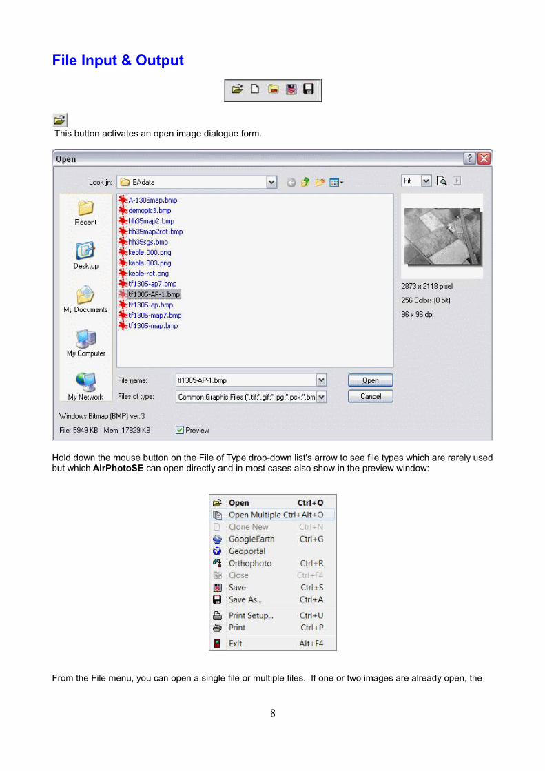
This button activates an open image dialogue form.

Hold down the mouse button on the File of Type drop-down list's arrow to see file types which are rarely usedbut which AirPhotoSE can open directly and in most cases also show in the preview window:

From the File menu, you can open a single file or multiple files. If one or two images are already open, the

8

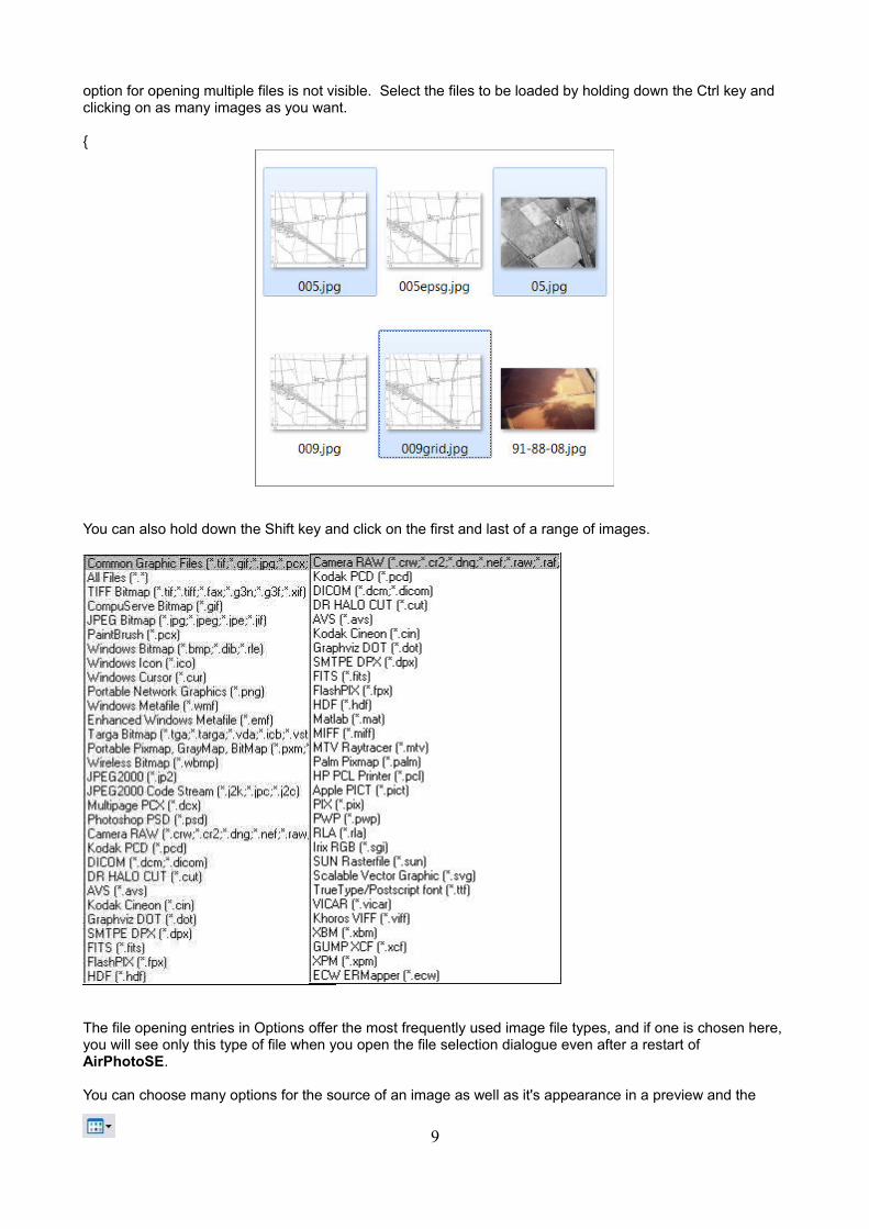
option for opening multiple files is not visible. Select the files to be loaded by holding down the Ctrl key and clicking on as many images as you want.

{

You can also hold down the Shift key and click on the first and last of a range of images.

The file opening entries in Options offer the most frequently used image file types, and if one is chosen here, you will see only this type of file when you open the file selection dialogue even after a restart of AirPhotoSE.

You can choose many options for the source of an image as well as it's appearance in a preview and the

9

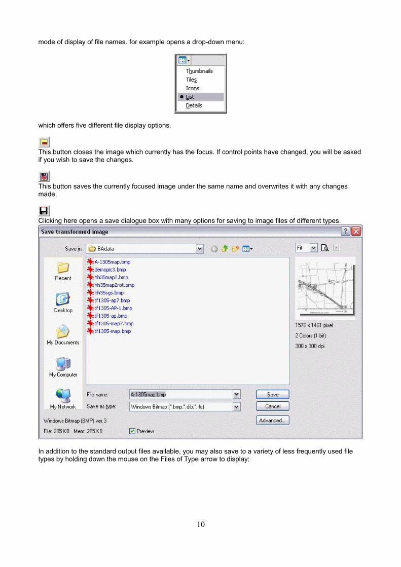
mode of display of file names. for example opens a drop-down menu:

which offers five different file display options.

This button closes the image which currently has the focus. If control points have changed, you will be askedif you wish to save the changes.

This button saves the currently focused image under the same name and overwrites it with any changes made.

Clicking here opens a save dialogue box with many options for saving to image files of different types.

In addition to the standard output files available, you may also save to a variety of less frequently used file types by holding down the mouse on the Files of Type arrow to display:

10

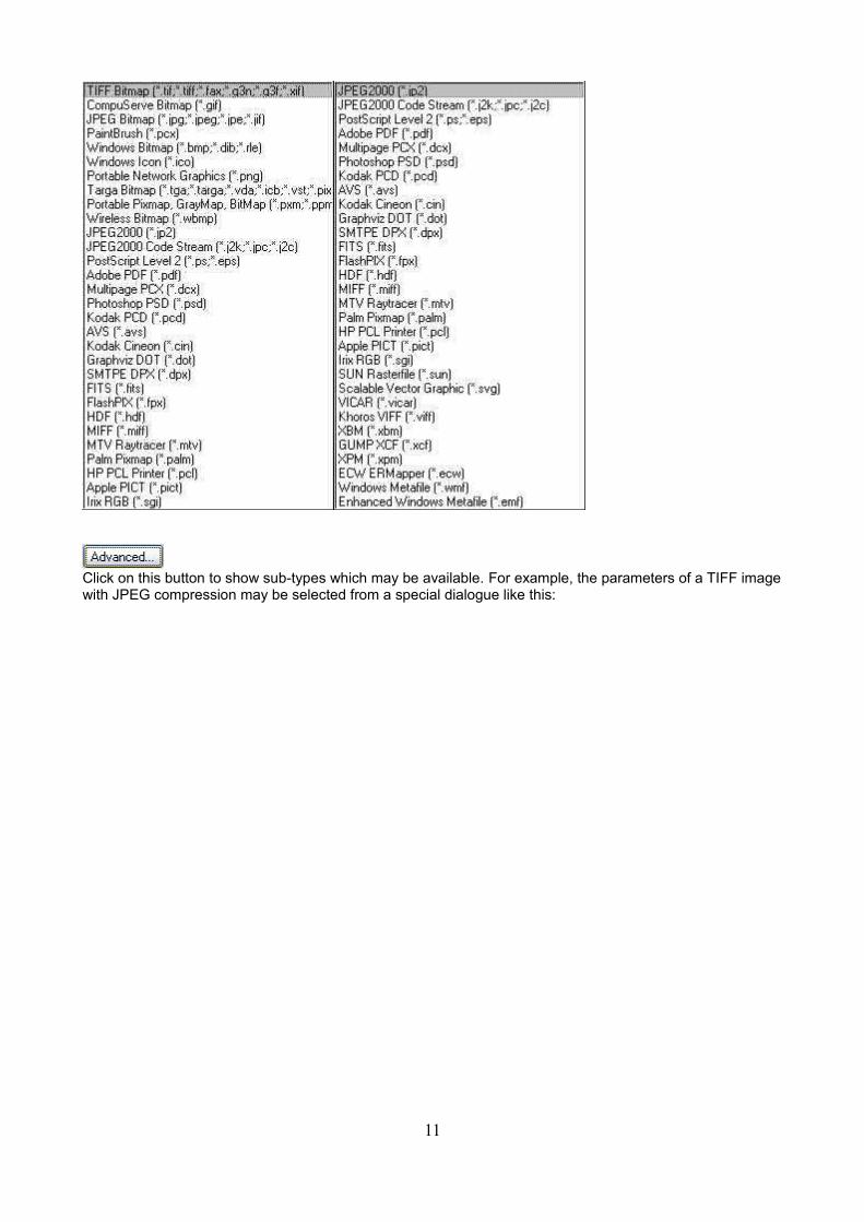
Click on this button to show sub-types which may be available. For example, the parameters of a TIFF imagewith JPEG compression may be selected from a special dialogue like this:

11

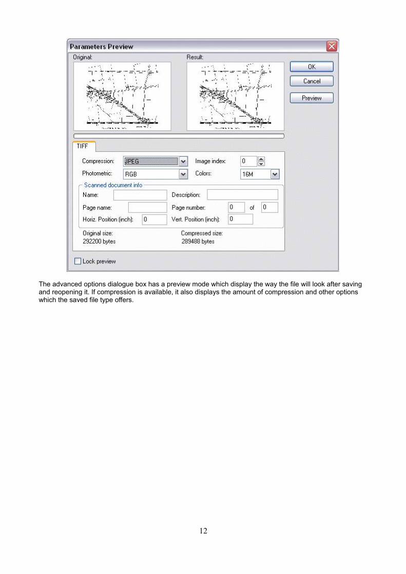
The advanced options dialogue box has a preview mode which display the way the file will look after saving and reopening it. If compression is available, it also displays the amount of compression and other options which the saved file type offers.

12

Toolbars and Menus

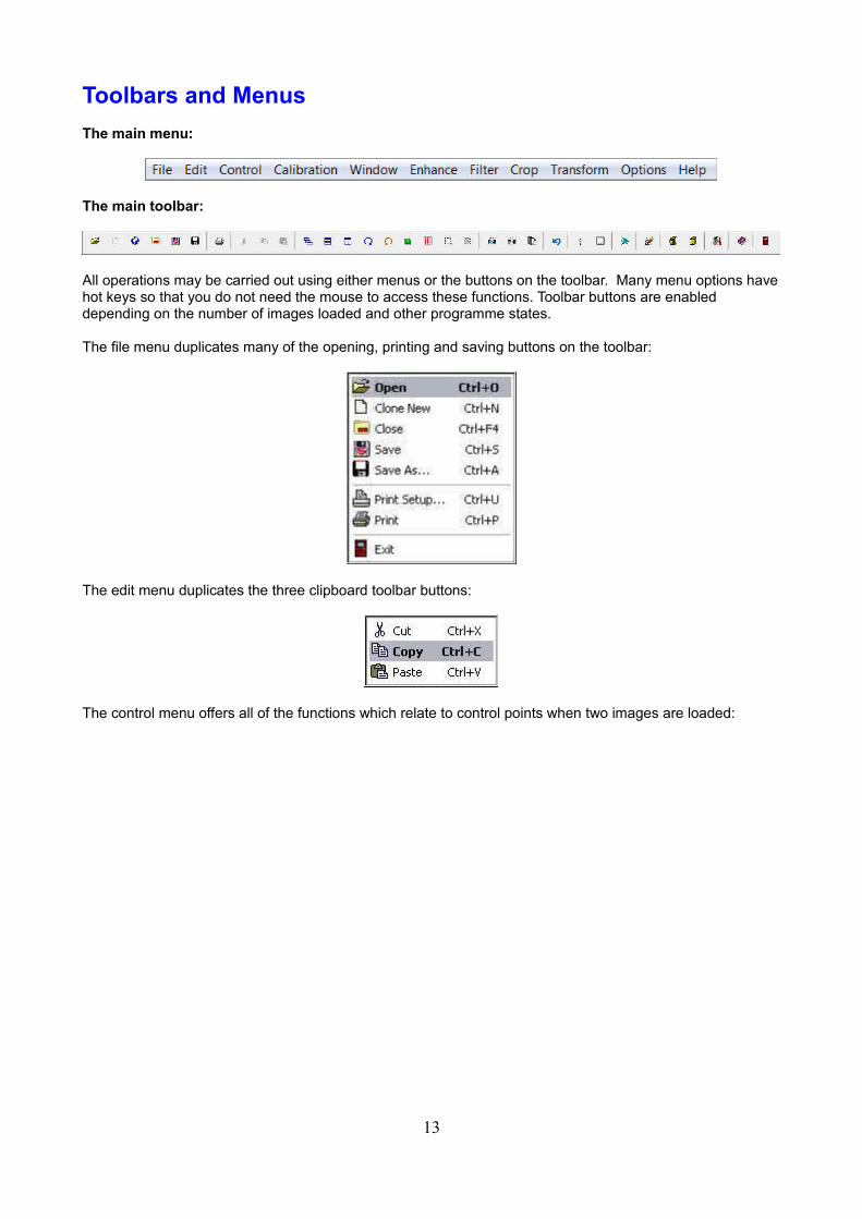
The main menu:

The main toolbar:

All operations may be carried out using either menus or the buttons on the toolbar. Many menu options havehot keys so that you do not need the mouse to access these functions. Toolbar buttons are enabled depending on the number of images loaded and other programme states.

The file menu duplicates many of the opening, printing and saving buttons on the toolbar:

The edit menu duplicates the three clipboard toolbar buttons:

The control menu offers all of the functions which relate to control points when two images are loaded:

13

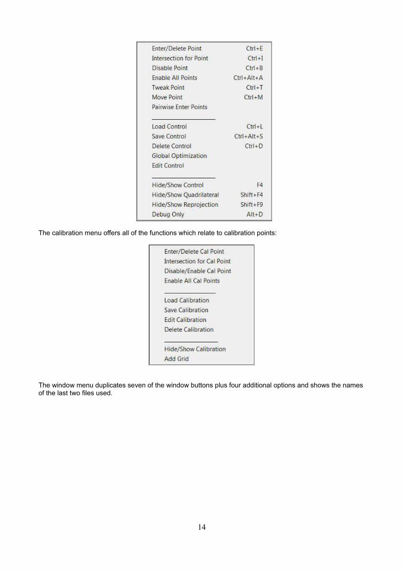
The calibration menu offers all of the functions which relate to calibration points:

The window menu duplicates seven of the window buttons plus four additional options and shows the namesof the last two files used.

14

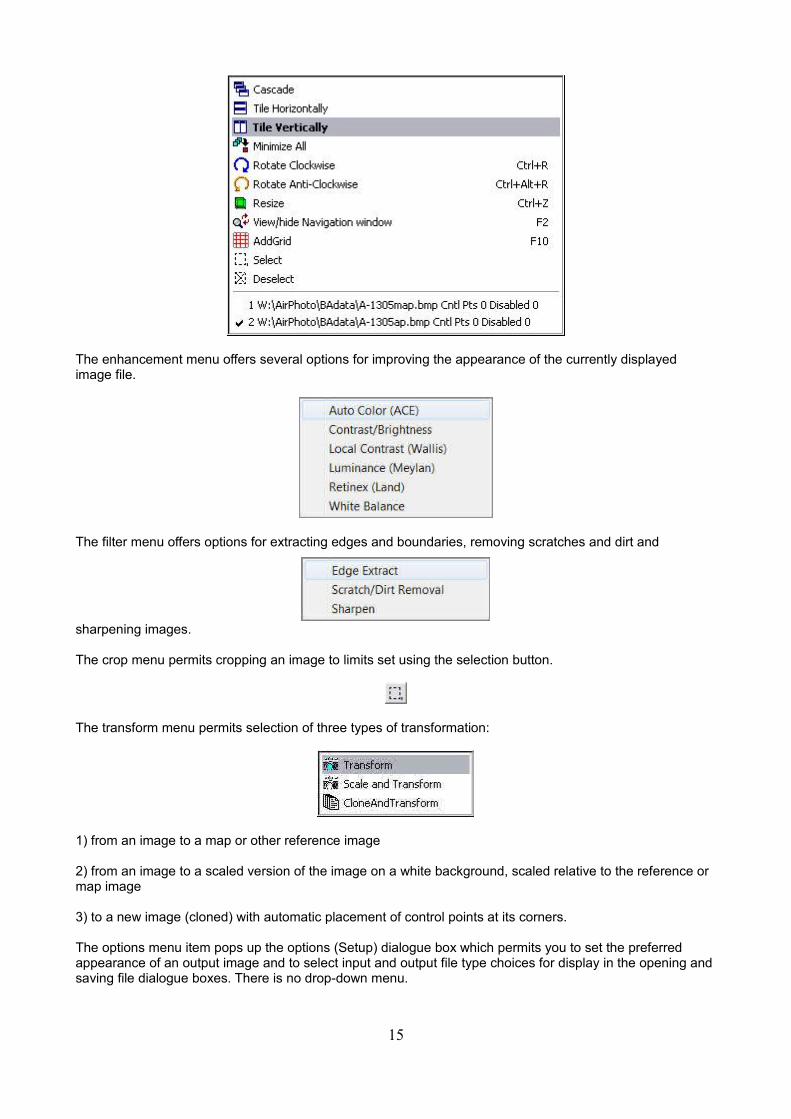
The enhancement menu offers several options for improving the appearance of the currently displayed image file.

The filter menu offers options for extracting edges and boundaries, removing scratches and dirt and

sharpening images.

The crop menu permits cropping an image to limits set using the selection button.

The transform menu permits selection of three types of transformation:

1) from an image to a map or other reference image

2) from an image to a scaled version of the image on a white background, scaled relative to the reference or map image

3) to a new image (cloned) with automatic placement of control points at its corners.

The options menu item pops up the options (Setup) dialogue box which permits you to set the preferred appearance of an output image and to select input and output file type choices for display in the opening andsaving file dialogue boxes. There is no drop-down menu.

15

The help menu provides access to the full help contents, the copyright, version and build notice in the About dialogue, and it offers an option to check for an update for the programme and download it directly from the Internet if one is available.

16

Control Points

At least four control points are required for calculating the transformation parameters (called a Homography in the computer vision literature) between two images or an image and a map. Each point in each image is given a unique number, and these must correspond. You may add as many control points as you wish.

Warning:

More than four control points may or may not improve the accuracy of the transformation. Small differences in position can't always be seen visually, but they make an enormous difference in the result when there are three control points which almost line up in the source and target images. That causes mathematical instability, and a single pixel displacement may produce an enormous shift or skew in a transformed image.

That's why some data behaves best when you use only four points, since the line-up problem doesn't exist. However, it is desirable that control points be spaced as widely as possible in the source image. Always startwith only four points and always add only one additional point at a time. Then try the transformation to see if things improve or get worse, and if the latter, either disable or remove the fifth point before adding a sixth one. Stop adding points when there is no visual improvement. It is wrong to think that simply adding more points will somehow make things better. Depending on the data and the terrain, this may be true, but more frequently it's not the case.

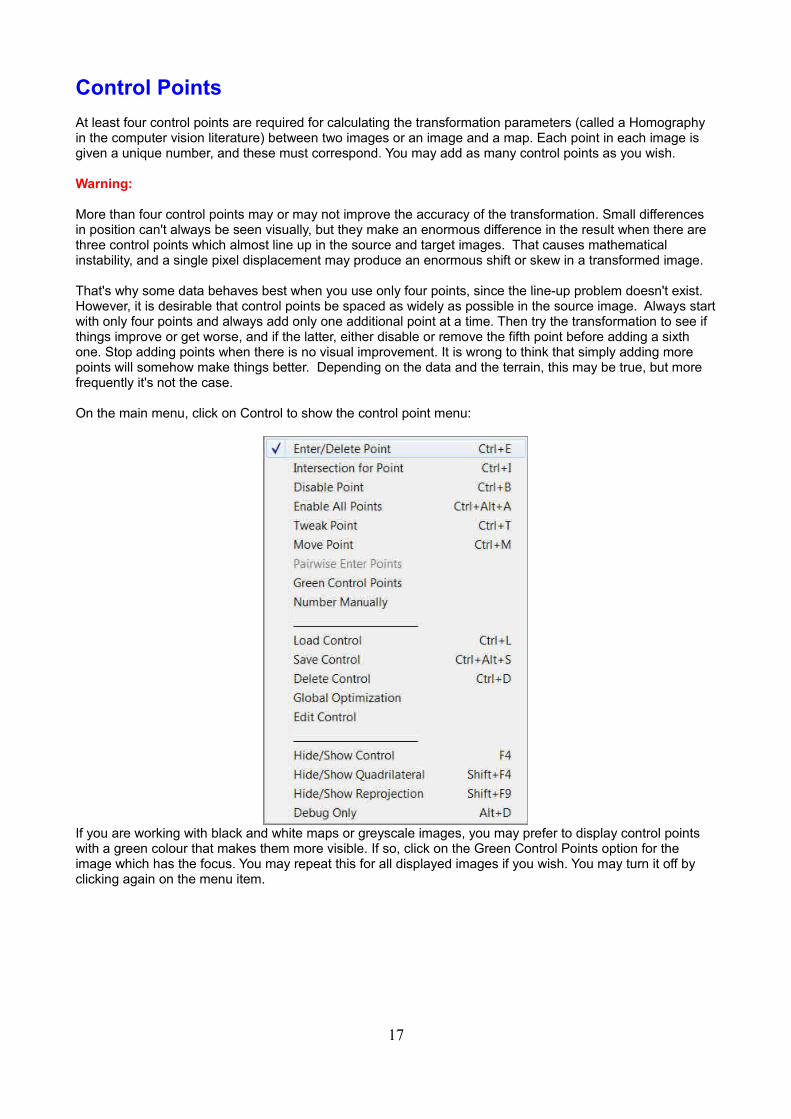
On the main menu, click on Control to show the control point menu:

If you are working with black and white maps or greyscale images, you may prefer to display control points with a green colour that makes them more visible. If so, click on the Green Control Points option for the image which has the focus. You may repeat this for all displayed images if you wish. You may turn it off by clicking again on the menu item.

17

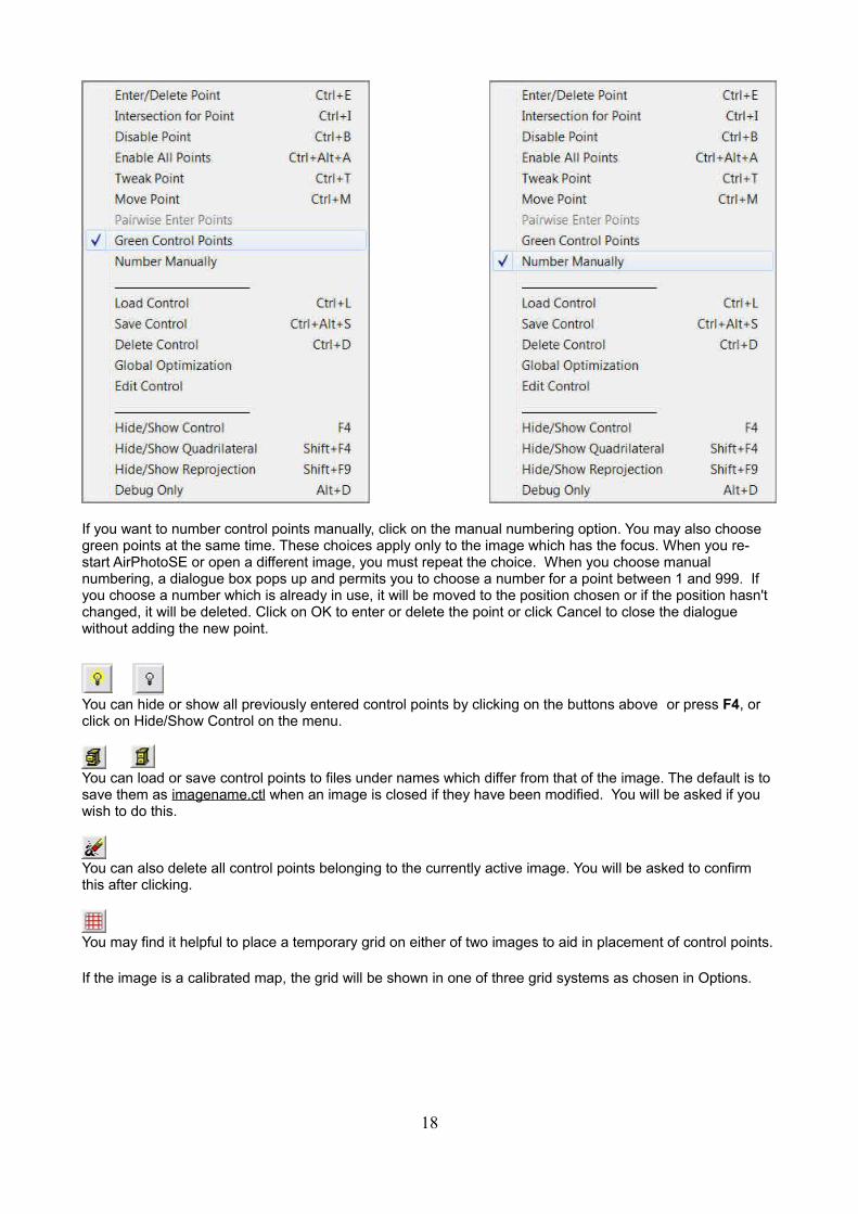
If you want to number control points manually, click on the manual numbering option. You may also choose green points at the same time. These choices apply only to the image which has the focus. When you re-start AirPhotoSE or open a different image, you must repeat the choice. When you choose manual numbering, a dialogue box pops up and permits you to choose a number for a point between 1 and 999. If you choose a number which is already in use, it will be moved to the position chosen or if the position hasn't changed, it will be deleted. Click on OK to enter or delete the point or click Cancel to close the dialogue without adding the new point.

You can hide or show all previously entered control points by clicking on the buttons above or press F4, or click on Hide/Show Control on the menu.

You can load or save control points to files under names which differ from that of the image. The default is to save them as imagename.ctl when an image is closed if they have been modified. You will be asked if you wish to do this.

You can also delete all control points belonging to the currently active image. You will be asked to confirm this after clicking.

You may find it helpful to place a temporary grid on either of two images to aid in placement of control points.

If the image is a calibrated map, the grid will be shown in one of three grid systems as chosen in Options.

18

The following operations can be performed on control points in one or two images:

Enter or Delete a single control point:

From the Control menu choose:

Enter

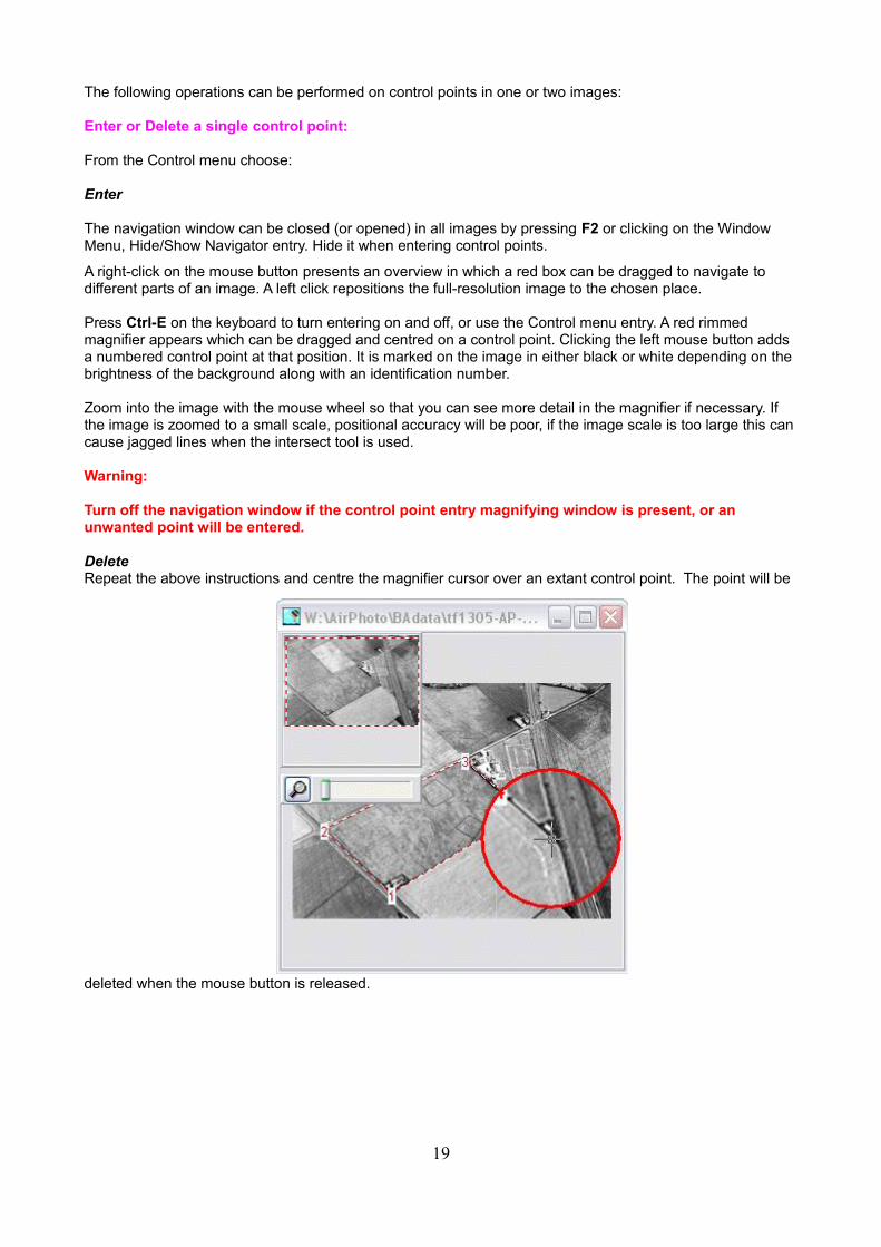
The navigation window can be closed (or opened) in all images by pressing F2 or clicking on the Window Menu, Hide/Show Navigator entry. Hide it when entering control points.

A right-click on the mouse button presents an overview in which a red box can be dragged to navigate to different parts of an image. A left click repositions the full-resolution image to the chosen place.

Press Ctrl-E on the keyboard to turn entering on and off, or use the Control menu entry. A red rimmed magnifier appears which can be dragged and centred on a control point. Clicking the left mouse button adds a numbered control point at that position. It is marked on the image in either black or white depending on the brightness of the background along with an identification number.

Zoom into the image with the mouse wheel so that you can see more detail in the magnifier if necessary. If the image is zoomed to a small scale, positional accuracy will be poor, if the image scale is too large this cancause jagged lines when the intersect tool is used.

Warning:

Turn off the navigation window if the control point entry magnifying window is present, or an unwanted point will be entered.

DeleteRepeat the above instructions and centre the magnifier cursor over an extant control point. The point will be

deleted when the mouse button is released.

19

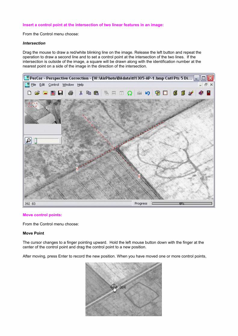
Insert a control point at the intersection of two linear features in an image:

From the Control menu choose:

Intersection

Drag the mouse to draw a red/white blinking line on the image. Release the left button and repeat the operation to draw a second line and to set a control point at the intersection of the two lines. If the intersection is outside of the image, a square will be drawn along with the identification number at the nearest point on a side of the image in the direction of the intersection.

Move control points:

From the Control menu choose:

Move Point

The cursor changes to a finger pointing upward. Hold the left mouse button down with the finger at the center of the control point and drag the control point to a new position.

After moving, press Enter to record the new position. When you have moved one or more control points,

20

press Enter for each one. When finished, uncheck the Move item on the Control menu.

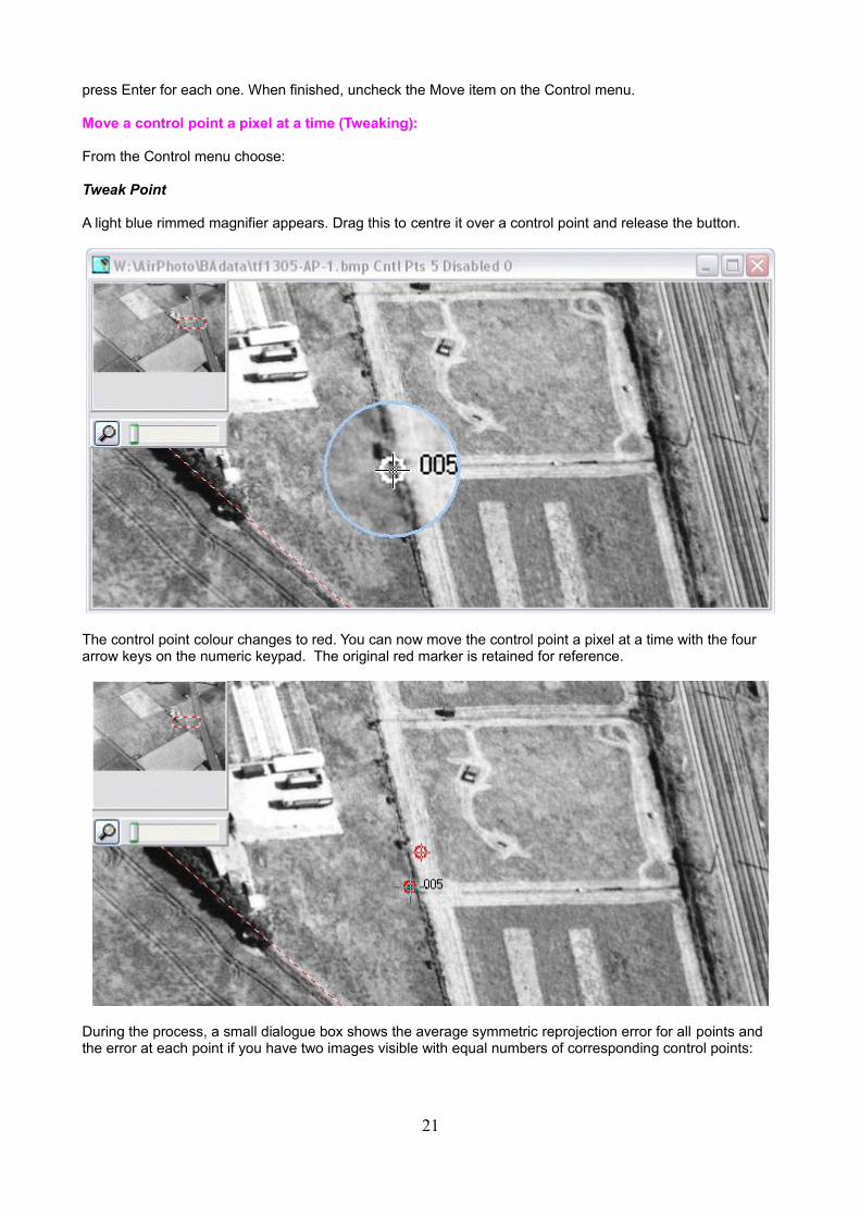
Move a control point a pixel at a time (Tweaking):

From the Control menu choose:

Tweak Point

A light blue rimmed magnifier appears. Drag this to centre it over a control point and release the button.

The control point colour changes to red. You can now move the control point a pixel at a time with the four arrow keys on the numeric keypad. The original red marker is retained for reference.

During the process, a small dialogue box shows the average symmetric reprojection error for all points and the error at each point if you have two images visible with equal numbers of corresponding control points:

21

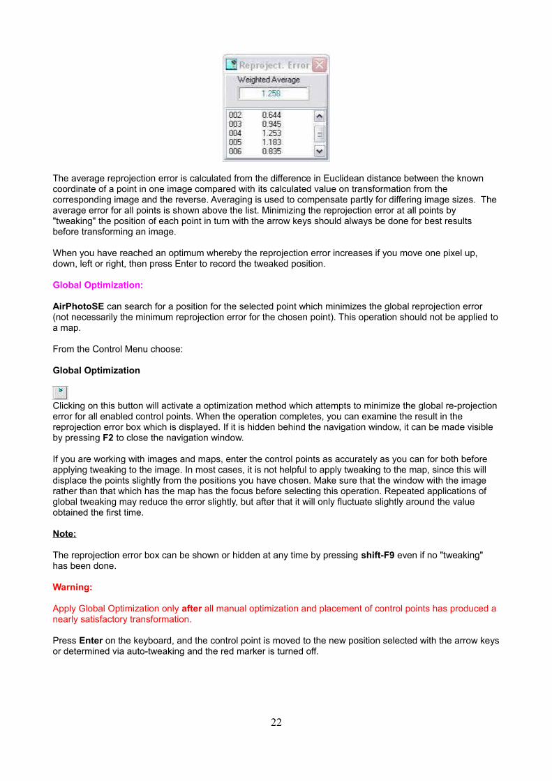
The average reprojection error is calculated from the difference in Euclidean distance between the known coordinate of a point in one image compared with its calculated value on transformation from the corresponding image and the reverse. Averaging is used to compensate partly for differing image sizes. The average error for all points is shown above the list. Minimizing the reprojection error at all points by "tweaking" the position of each point in turn with the arrow keys should always be done for best results before transforming an image.

When you have reached an optimum whereby the reprojection error increases if you move one pixel up, down, left or right, then press Enter to record the tweaked position.

Global Optimization:

AirPhotoSE can search for a position for the selected point which minimizes the global reprojection error (not necessarily the minimum reprojection error for the chosen point). This operation should not be applied toa map.

From the Control Menu choose:

Global Optimization

Clicking on this button will activate a optimization method which attempts to minimize the global re-projectionerror for all enabled control points. When the operation completes, you can examine the result in the reprojection error box which is displayed. If it is hidden behind the navigation window, it can be made visible by pressing F2 to close the navigation window.

If you are working with images and maps, enter the control points as accurately as you can for both before applying tweaking to the image. In most cases, it is not helpful to apply tweaking to the map, since this will displace the points slightly from the positions you have chosen. Make sure that the window with the image rather than that which has the map has the focus before selecting this operation. Repeated applications of global tweaking may reduce the error slightly, but after that it will only fluctuate slightly around the value obtained the first time.

Note:

The reprojection error box can be shown or hidden at any time by pressing shift-F9 even if no "tweaking" has been done.

Warning:

Apply Global Optimization only after all manual optimization and placement of control points has produced a nearly satisfactory transformation.

Press Enter on the keyboard, and the control point is moved to the new position selected with the arrow keysor determined via auto-tweaking and the red marker is turned off.

22

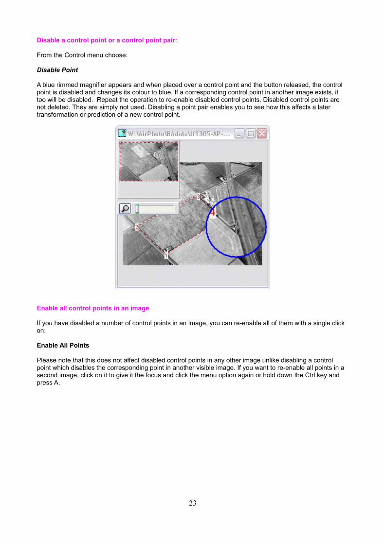
Disable a control point or a control point pair:

From the Control menu choose:

Disable Point

A blue rimmed magnifier appears and when placed over a control point and the button released, the control point is disabled and changes its colour to blue. If a corresponding control point in another image exists, it too will be disabled. Repeat the operation to re-enable disabled control points. Disabled control points are not deleted. They are simply not used. Disabling a point pair enables you to see how this affects a later transformation or prediction of a new control point.

Enable all control points in an image

If you have disabled a number of control points in an image, you can re-enable all of them with a single click on:

Enable All Points

Please note that this does not affect disabled control points in any other image unlike disabling a control point which disables the corresponding point in another visible image. If you want to re-enable all points in a second image, click on it to give it the focus and click the menu option again or hold down the Ctrl key and press A.

23

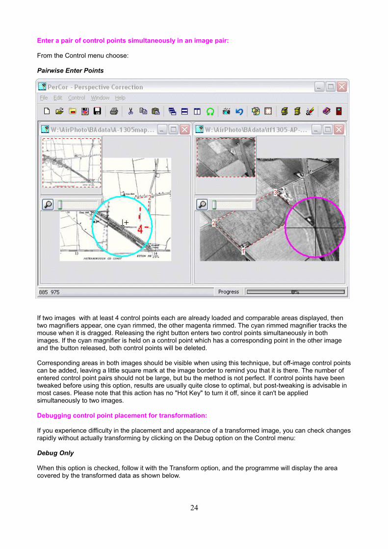
Enter a pair of control points simultaneously in an image pair:

From the Control menu choose:

Pairwise Enter Points

If two images with at least 4 control points each are already loaded and comparable areas displayed, then two magnifiers appear, one cyan rimmed, the other magenta rimmed. The cyan rimmed magnifier tracks the mouse when it is dragged. Releasing the right button enters two control points simultaneously in both images. If the cyan magnifier is held on a control point which has a corresponding point in the other image and the button released, both control points will be deleted.

Corresponding areas in both images should be visible when using this technique, but off-image control pointscan be added, leaving a little square mark at the image border to remind you that it is there. The number of entered control point pairs should not be large, but bu the method is not perfect. If control points have been tweaked before using this option, results are usually quite close to optimal, but post-tweaking is advisable in most cases. Please note that this action has no "Hot Key" to turn it off, since it can't be applied simultaneously to two images.

Debugging control point placement for transformation:

If you experience difficulty in the placement and appearance of a transformed image, you can check changesrapidly without actually transforming by clicking on the Debug option on the Control menu:

Debug Only

When this option is checked, follow it with the Transform option, and the programme will display the area covered by the transformed data as shown below.

24

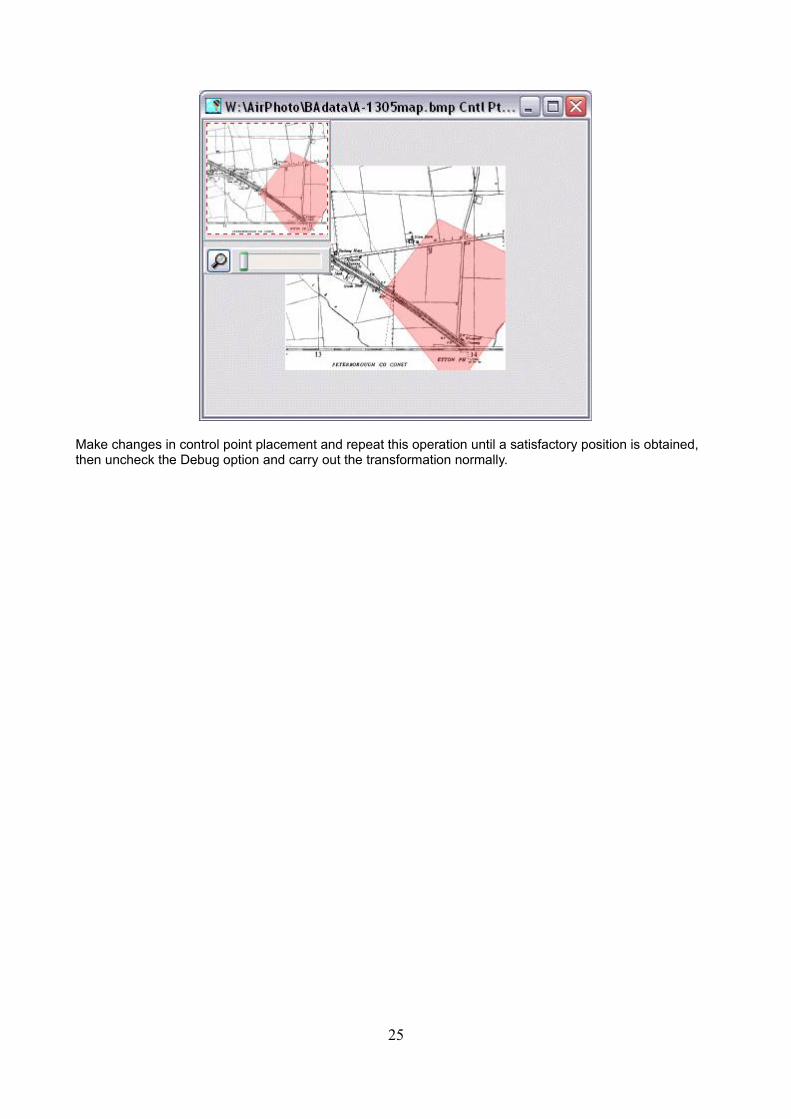
Make changes in control point placement and repeat this operation until a satisfactory position is obtained, then uncheck the Debug option and carry out the transformation normally.

25

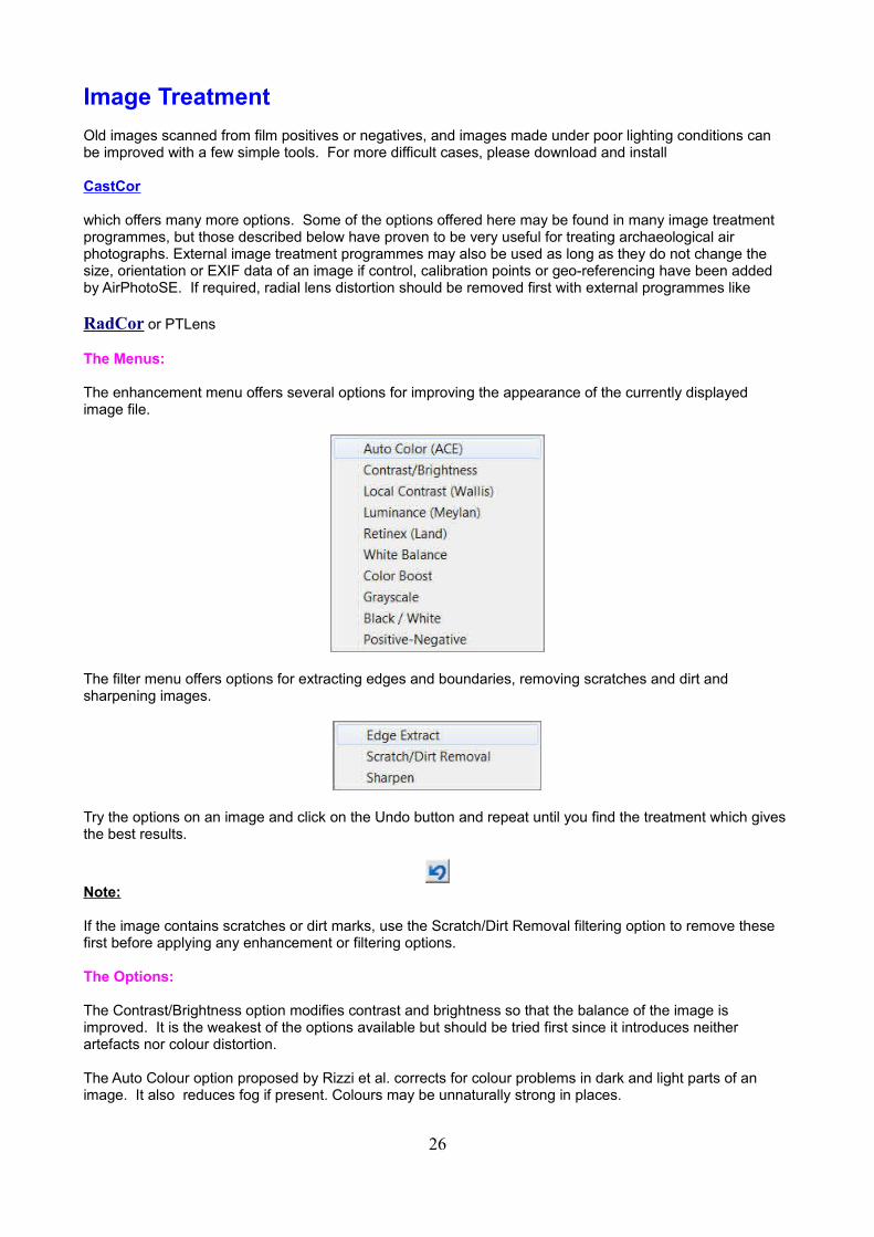
Image Treatment

Old images scanned from film positives or negatives, and images made under poor lighting conditions can be improved with a few simple tools. For more difficult cases, please download and install

CastCor

which offers many more options. Some of the options offered here may be found in many image treatment programmes, but those described below have proven to be very useful for treating archaeological air photographs. External image treatment programmes may also be used as long as they do not change the size, orientation or EXIF data of an image if control, calibration points or geo-referencing have been added by AirPhotoSE. If required, radial lens distortion should be removed first with external programmes like

RadCor or PTLens

The Menus:

The enhancement menu offers several options for improving the appearance of the currently displayed image file.

The filter menu offers options for extracting edges and boundaries, removing scratches and dirt and sharpening images.

Try the options on an image and click on the Undo button and repeat until you find the treatment which gives the best results.

Note:

If the image contains scratches or dirt marks, use the Scratch/Dirt Removal filtering option to remove these first before applying any enhancement or filtering options.

The Options:

The Contrast/Brightness option modifies contrast and brightness so that the balance of the image is improved. It is the weakest of the options available but should be tried first since it introduces neither artefacts nor colour distortion.

The Auto Colour option proposed by Rizzi et al. corrects for colour problems in dark and light parts of an image. It also reduces fog if present. Colours may be unnaturally strong in places.

26

The Luminance option due to Meylan greatly improves the visibility of fine structure in dark parts of an image without affecting the remainder.

The Retinex method, proposed by Edwin Land, the inventor of the Polaroid process and as implemented by Barnard is much stronger and also works on the light areas. Colours are distorted.

Local Adaptive Contrast due to Wallis improves the visibility of fine structure in the whole image and sharpens it at the same time. It does not affect the colours.

The White Balance option corrects for colour cast automatically by computing an optimal white point and modifying the colours of all pixels.

Colour Boost using Van de Weijer's algorithm exaggerates colour differences, giving an image a false-colour film appearance. This may be useful as a preliminary step for images where luminance differences along boundaries are weak. Buildings and roads are usually sharpened considerably. Archaeological markings are less visible, so after placing control points, back off with the Undo button and save the original with the new control points.

Gray-scale converts a colour image to a grayscale image.

Black / White converts a colour or grayscale image to a black and white image. Weak fine grey lines are enhanced for greater visibility.

The options may be applied in any sequence. The Undo button may be clicked on to go back one step if the result is not useful. The edge extraction filter may give better results after a combination of several of the enhancement options.

See the bibliography for detailed references for the enhancement and filtering options.

27

Transformation

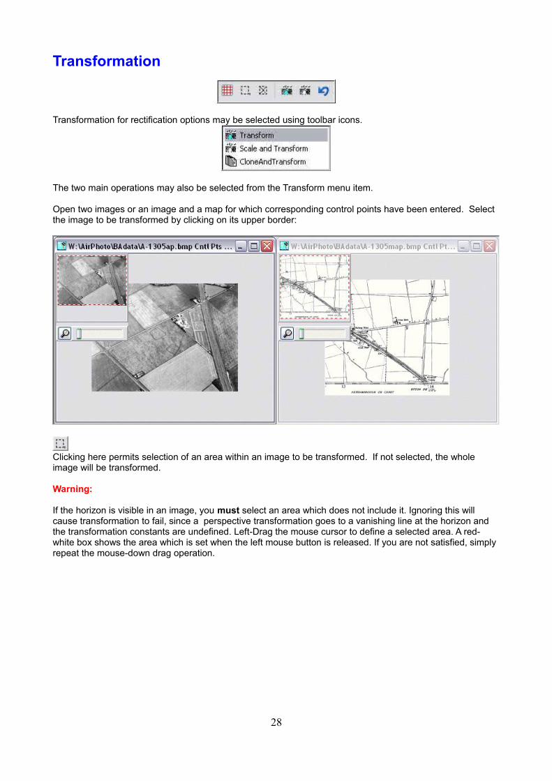
Transformation for rectification options may be selected using toolbar icons.

The two main operations may also be selected from the Transform menu item.

Open two images or an image and a map for which corresponding control points have been entered. Select the image to be transformed by clicking on its upper border:

Clicking here permits selection of an area within an image to be transformed. If not selected, the whole image will be transformed.

Warning:

If the horizon is visible in an image, you must select an area which does not include it. Ignoring this will cause transformation to fail, since a perspective transformation goes to a vanishing line at the horizon and the transformation constants are undefined. Left-Drag the mouse cursor to define a selected area. A red-white box shows the area which is set when the left mouse button is released. If you are not satisfied, simply repeat the mouse-down drag operation.

28

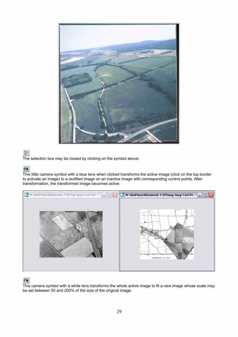
The selection box may be closed by clicking on the symbol above.

This little camera symbol with a blue lens when clicked transforms the active image (click on the top border to activate an image) to a rectified image on an inactive image with corresponding control points. After transformation, the transformed image becomes active.

This camera symbol with a white lens transforms the whole active image to fit a new image whose scale maybe set between 50 and 200% of the size of the original image.

29

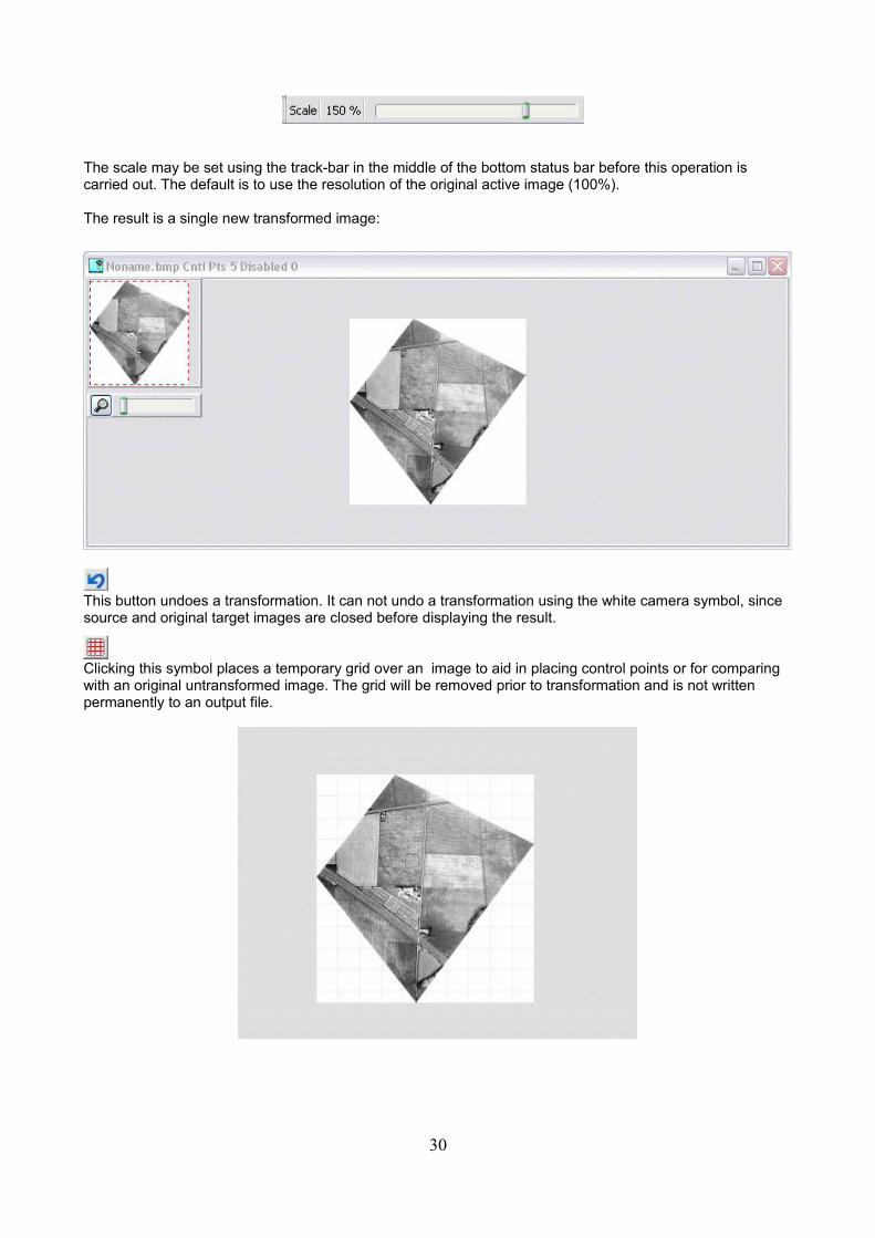
The scale may be set using the track-bar in the middle of the bottom status bar before this operation is carried out. The default is to use the resolution of the original active image (100%).

The result is a single new transformed image:

This button undoes a transformation. It can not undo a transformation using the white camera symbol, since source and original target images are closed before displaying the result.

Clicking this symbol places a temporary grid over an image to aid in placing control points or for comparing with an original untransformed image. The grid will be removed prior to transformation and is not written permanently to an output file.

30

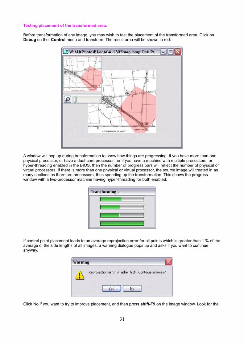
Testing placement of the transformed area:

Before transformation of any image, you may wish to test the placement of the transformed area. Click on Debug on the Control menu and transform. The result area will be shown in red:

A window will pop up during transformation to show how things are progressing. If you have more than one physical processor, or have a dual-core processor, or if you have a machine with multiple processors or hyper-threading enabled in the BIOS, then the number of progress bars will reflect the number of physical or virtual processors. If there is more than one physical or virtual processor, the source image will treated in as many sections as there are processors, thus speeding up the transformation. This shows the progress window with a two-processor machine having hyper-threading for both enabled:

If control point placement leads to an average reprojection error for all points which is greater than 1 % of theaverage of the side lengths of all images, a warning dialogue pops up and asks if you want to continue anyway.

Click No if you want to try to improve placement, and then press shift-F9 on the image window. Look for the

31

control point with the highest error, then Alt - Right click on it and tweak it to reduce the error. Repeat this for the next highest error point and so on as described in the topic Move Control Points a Pixel at a Time in the Control Points chapter of this manual. Then try the transformation again.

Undo Notes:

Undoing a transformation permits choosing new parameters in Setup or modifying control points and re-transforming without re-loading everything. The undo function also turns off any area selection, grid and repaints the control points and the navigation palette of the original image. It may also be used on rotated and re-sampled images.

When Clone and transform is selected, the empty cloned window is shown after undo, leaving any control points intact. This window can then be resized if desired and the normal transformation operation repeated.

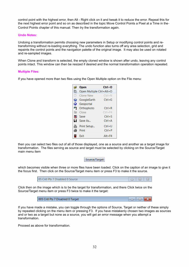
Multiple Files:

If you have opened more than two files using the Open Multiple option on the File menu:

then you can select two files out of all of those displayed, one as a source and another as a target image for transformation. The files serving as source and target must be selected by clicking on the Source/Target main menu item

which becomes visible when three or more files have been loaded. Click on the caption of an image to give itthe focus first. Then click on the Source/Target menu item or press F3 to make it the source.

Click then on the image which is to be the target for transformation, and there Click twice on the Source/Target menu item or press F3 twice to make it the target:

If you have made a mistake, you can toggle through the options of Source, Target or neither of these simply by repeated clicking on the menu item or pressing F3. If you have mistakenly chosen two images as sourcesand or two as a target but none as a source, you will get an error message when you attempt a transformation.

Proceed as above for transformation.

32

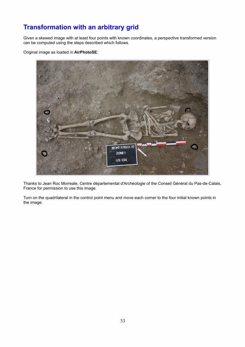
Transformation with an arbitrary grid

Given a skewed image with at least four points with known coordinates, a perspective transformed version can be computed using the steps described which follows.

Original image as loaded in AirPhotoSE:

Thanks to Jean Roc Morreale, Centre départemental d'Archéologie of the Conseil Général du Pas-de-Calais,France for permission to use this image.

Turn on the quadrilateral in the control point menu and move each corner to the four initial known points in the image:

33

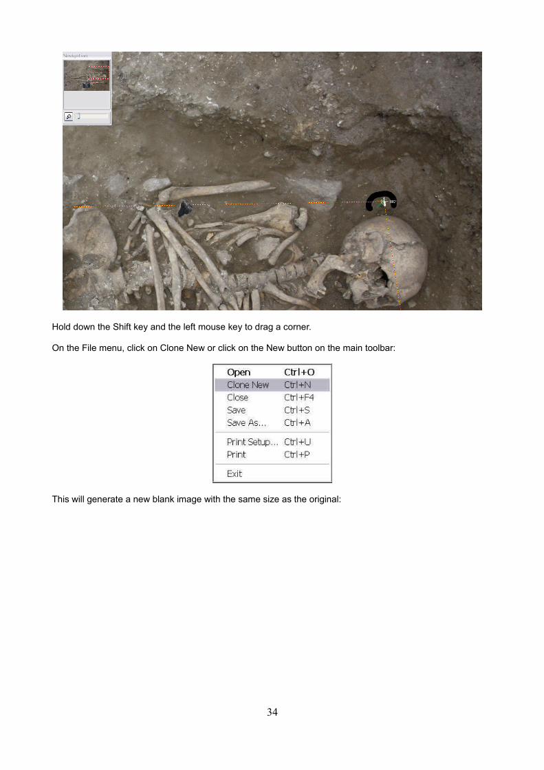
Hold down the Shift key and the left mouse key to drag a corner.

On the File menu, click on Clone New or click on the New button on the main toolbar:

This will generate a new blank image with the same size as the original:

34

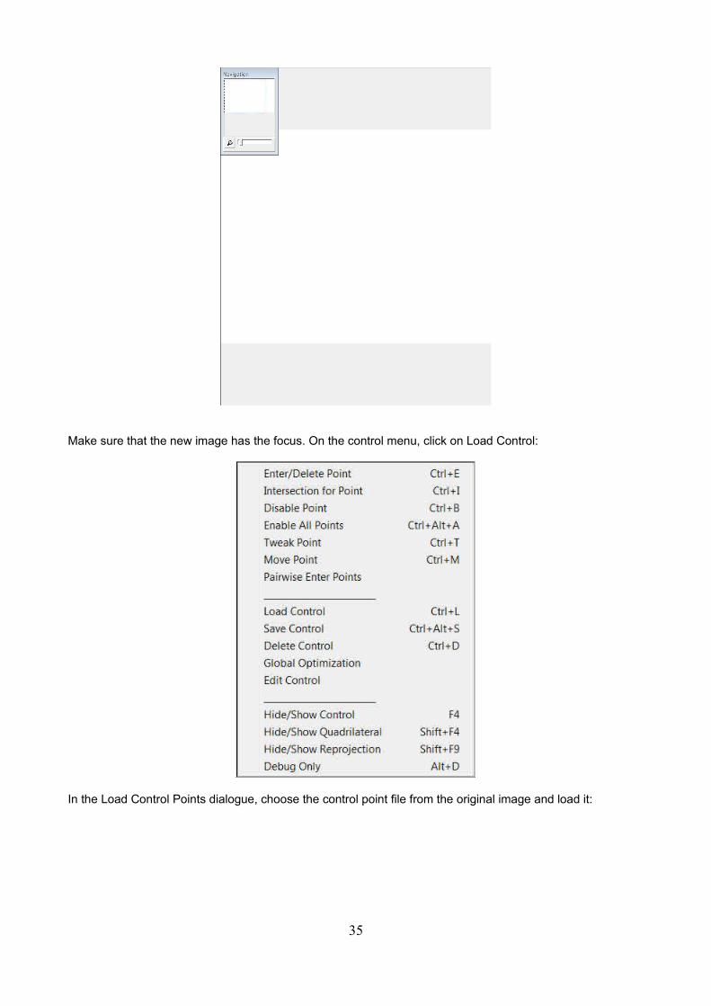
Make sure that the new image has the focus. On the control menu, click on Load Control:

In the Load Control Points dialogue, choose the control point file from the original image and load it:

35

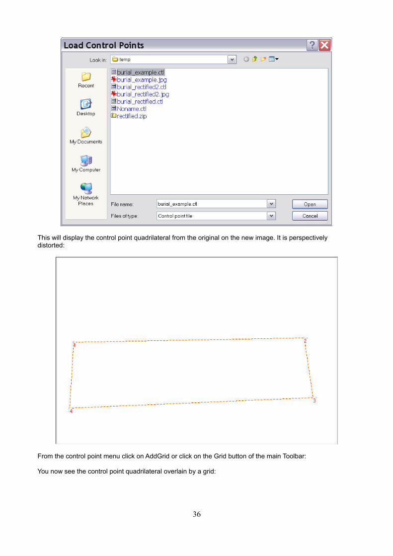
This will display the control point quadrilateral from the original on the new image. It is perspectively distorted:

From the control point menu click on AddGrid or click on the Grid button of the main Toolbar:

You now see the control point quadrilateral overlain by a grid:

36

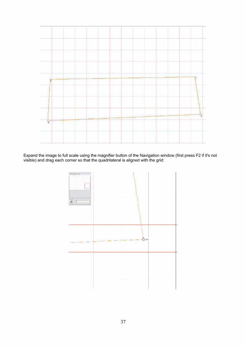
Expand the image to full scale using the magnifier button of the Navigation window (first press F2 if it's not visible) and drag each corner so that the quadrilateral is aligned with the grid:

37

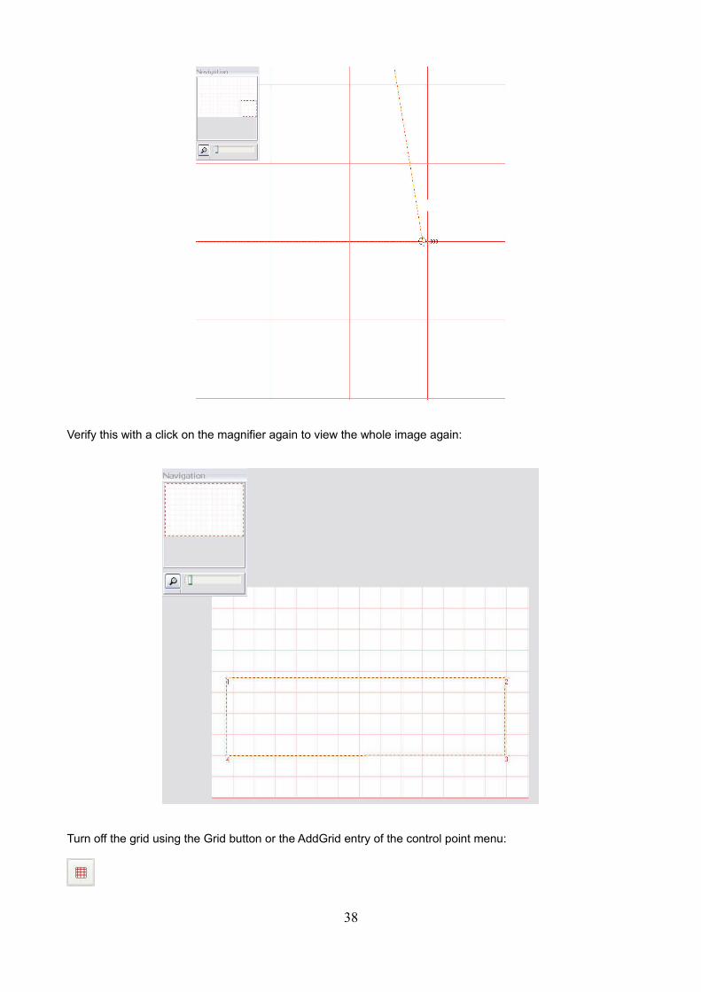
Verify this with a click on the magnifier again to view the whole image again:

Turn off the grid using the Grid button or the AddGrid entry of the control point menu:

38

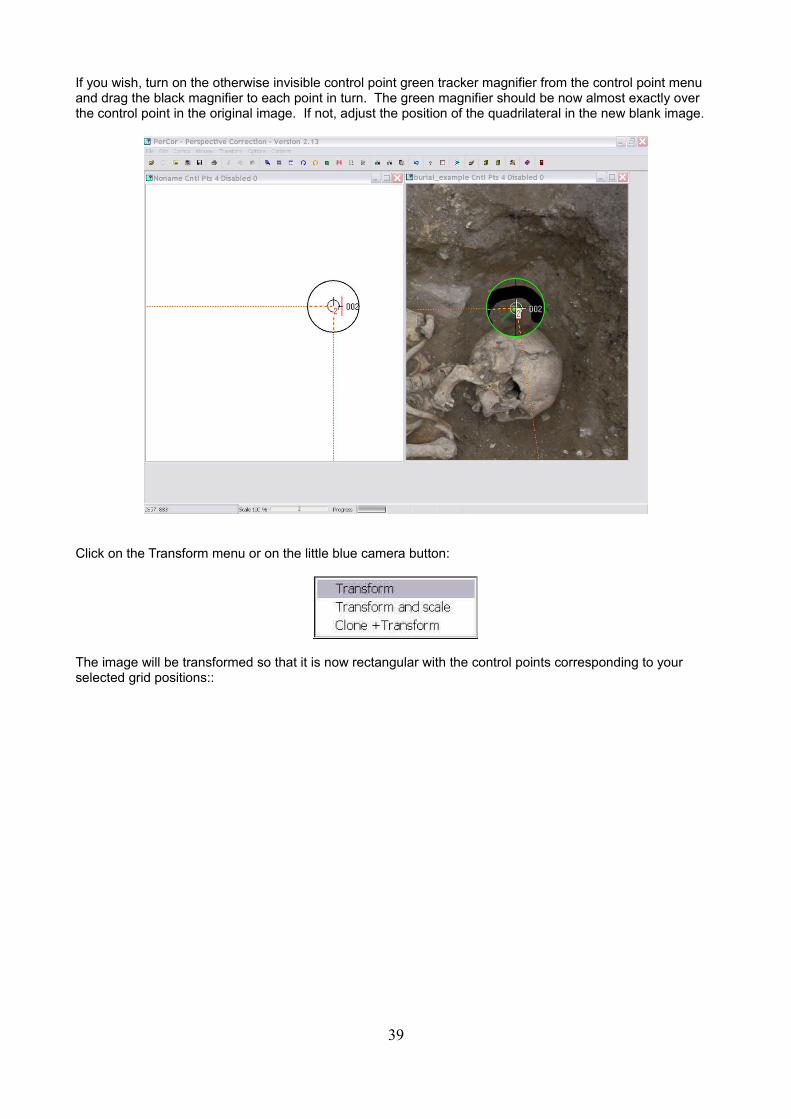
If you wish, turn on the otherwise invisible control point green tracker magnifier from the control point menu and drag the black magnifier to each point in turn. The green magnifier should be now almost exactly over the control point in the original image. If not, adjust the position of the quadrilateral in the new blank image.

Click on the Transform menu or on the little blue camera button:

The image will be transformed so that it is now rectangular with the control points corresponding to your selected grid positions::

39

40

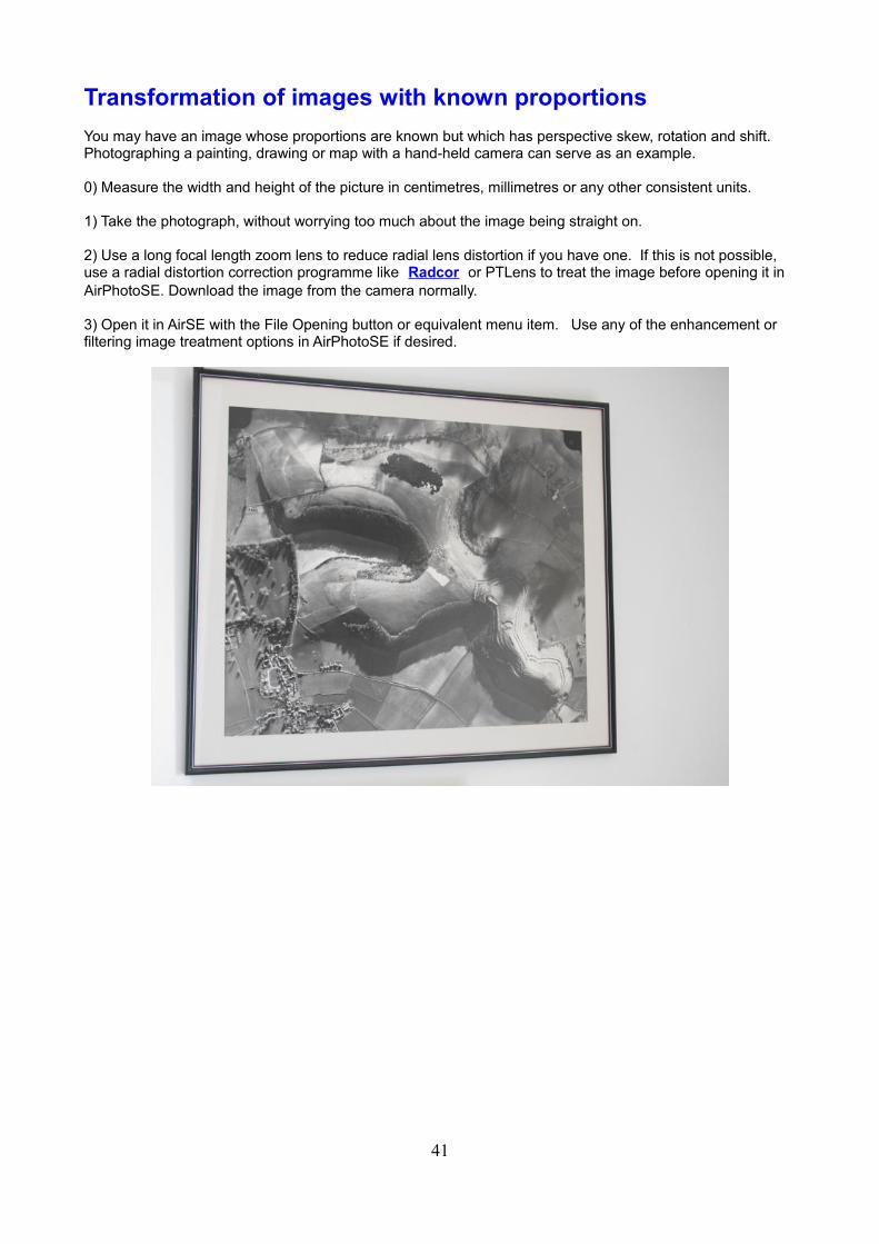
Transformation of images with known proportions

You may have an image whose proportions are known but which has perspective skew, rotation and shift. Photographing a painting, drawing or map with a hand-held camera can serve as an example.

0) Measure the width and height of the picture in centimetres, millimetres or any other consistent units.

1) Take the photograph, without worrying too much about the image being straight on.

2) Use a long focal length zoom lens to reduce radial lens distortion if you have one. If this is not possible, use a radial distortion correction programme like Radcor or PTLens to treat the image before opening it in AirPhotoSE. Download the image from the camera normally.

3) Open it in AirSE with the File Opening button or equivalent menu item. Use any of the enhancement or filtering image treatment options in AirPhotoSE if desired.

41

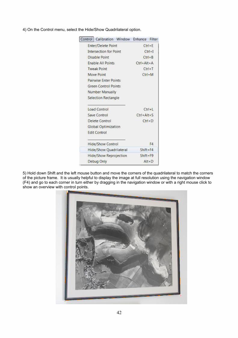
4) On the Control menu, select the Hide/Show Quadrilateral option.

5) Hold down Shift and the left mouse button and move the corners of the quadrilateral to match the corners of the picture frame. It is usually helpful to display the image at full resolution using the navigation window (F4) and go to each corner in turn either by dragging in the navigation window or with a right mouse click to show an overview with control points.

42

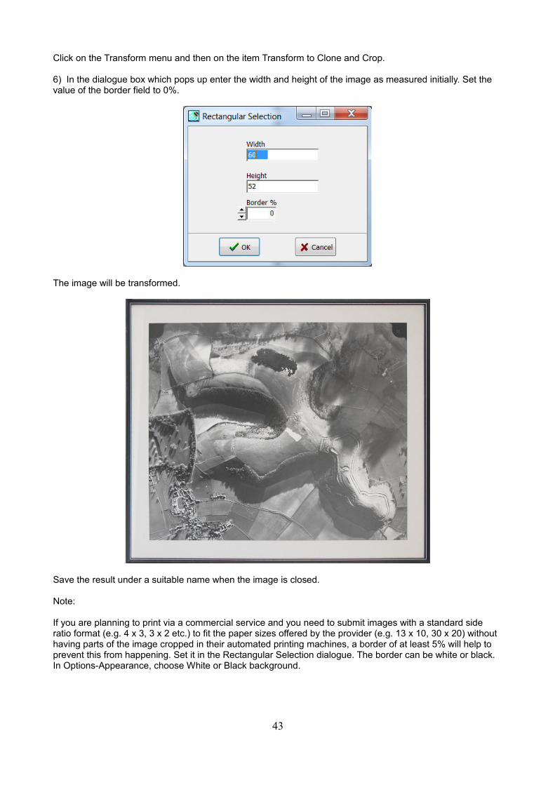
Click on the Transform menu and then on the item Transform to Clone and Crop.

6) In the dialogue box which pops up enter the width and height of the image as measured initially. Set the value of the border field to 0%.

The image will be transformed.

Save the result under a suitable name when the image is closed.

Note:

If you are planning to print via a commercial service and you need to submit images with a standard side ratio format (e.g. 4 x 3, 3 x 2 etc.) to fit the paper sizes offered by the provider (e.g. 13 x 10, 30 x 20) without having parts of the image cropped in their automated printing machines, a border of at least 5% will help to prevent this from happening. Set it in the Rectangular Selection dialogue. The border can be white or black. In Options-Appearance, choose White or Black background.

43

Transformation with Total Station Coordinates

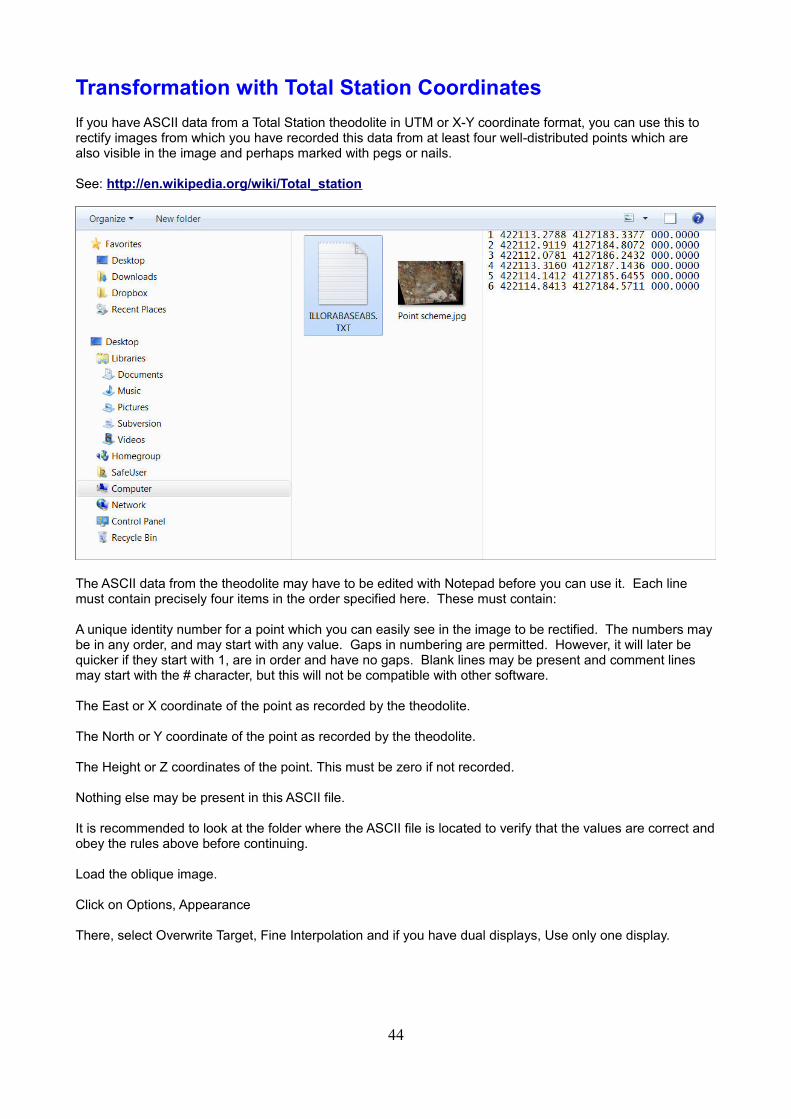
If you have ASCII data from a Total Station theodolite in UTM or X-Y coordinate format, you can use this to rectify images from which you have recorded this data from at least four well-distributed points which are also visible in the image and perhaps marked with pegs or nails.

See: http://en.wikipedia.org/wiki/Total_station

The ASCII data from the theodolite may have to be edited with Notepad before you can use it. Each line must contain precisely four items in the order specified here. These must contain:

A unique identity number for a point which you can easily see in the image to be rectified. The numbers maybe in any order, and may start with any value. Gaps in numbering are permitted. However, it will later be quicker if they start with 1, are in order and have no gaps. Blank lines may be present and comment lines may start with the # character, but this will not be compatible with other software.

The East or X coordinate of the point as recorded by the theodolite.

The North or Y coordinate of the point as recorded by the theodolite. The Height or Z coordinates of the point. This must be zero if not recorded.

Nothing else may be present in this ASCII file.

It is recommended to look at the folder where the ASCII file is located to verify that the values are correct andobey the rules above before continuing.

Load the oblique image.

Click on Options, Appearance

There, select Overwrite Target, Fine Interpolation and if you have dual displays, Use only one display.

44

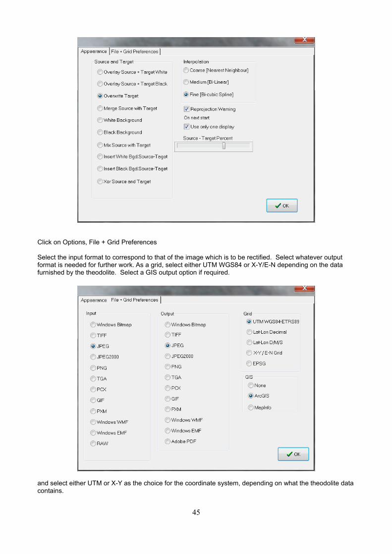
Click on Options, File + Grid Preferences

Select the input format to correspond to that of the image which is to be rectified. Select whatever output format is needed for further work. As a grid, select either UTM WGS84 or X-Y/E-N depending on the data furnished by the theodolite. Select a GIS output option if required.

and select either UTM or X-Y as the choice for the coordinate system, depending on what the theodolite datacontains.

45

Click OK

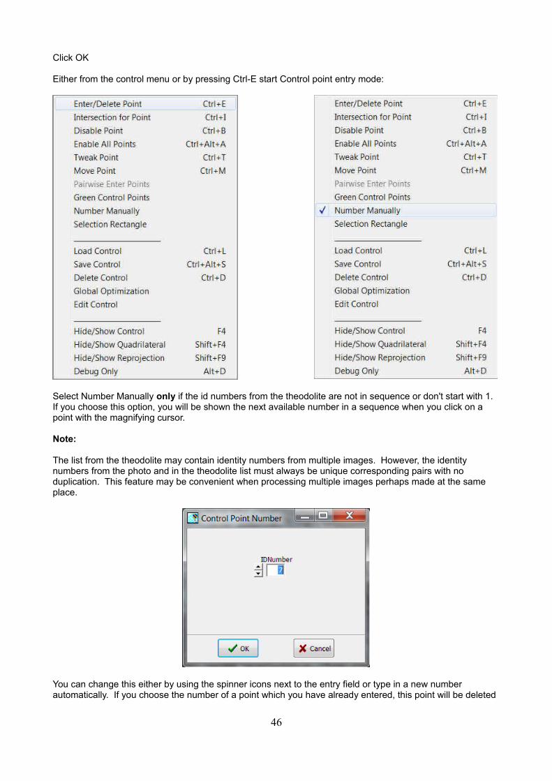
Either from the control menu or by pressing Ctrl-E start Control point entry mode:

Select Number Manually only if the id numbers from the theodolite are not in sequence or don't start with 1. If you choose this option, you will be shown the next available number in a sequence when you click on a point with the magnifying cursor.

Note:

The list from the theodolite may contain identity numbers from multiple images. However, the identity numbers from the photo and in the theodolite list must always be unique corresponding pairs with no duplication. This feature may be convenient when processing multiple images perhaps made at the same place.

You can change this either by using the spinner icons next to the entry field or type in a new number automatically. If you choose the number of a point which you have already entered, this point will be deleted

46

and a new point created. However, as stated above, it is faster not to use manual numbering provided that the ID numbers of the ASCII file from the theodolite are in simple ascending numerical order. Then, the default automatic control point numbering scheme in AirPhotoSE can be used.

Save the image using the Save As option after you have finished adding control points at all the places listed in the theodolite ASCII file.

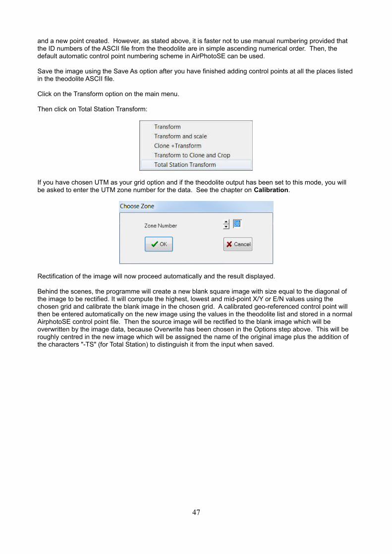
Click on the Transform option on the main menu.

Then click on Total Station Transform:

If you have chosen UTM as your grid option and if the theodolite output has been set to this mode, you will be asked to enter the UTM zone number for the data. See the chapter on Calibration.

Rectification of the image will now proceed automatically and the result displayed.

Behind the scenes, the programme will create a new blank square image with size equal to the diagonal of the image to be rectified. It will compute the highest, lowest and mid-point X/Y or E/N values using the chosen grid and calibrate the blank image in the chosen grid. A calibrated geo-referenced control point will then be entered automatically on the new image using the values in the theodolite list and stored in a normal AirphotoSE control point file. Then the source image will be rectified to the blank image which will be overwritten by the image data, because Overwrite has been chosen in the Options step above. This will be roughly centred in the new image which will be assigned the name of the original image plus the addition of the characters "-TS" (for Total Station) to distinguish it from the input when saved.

47

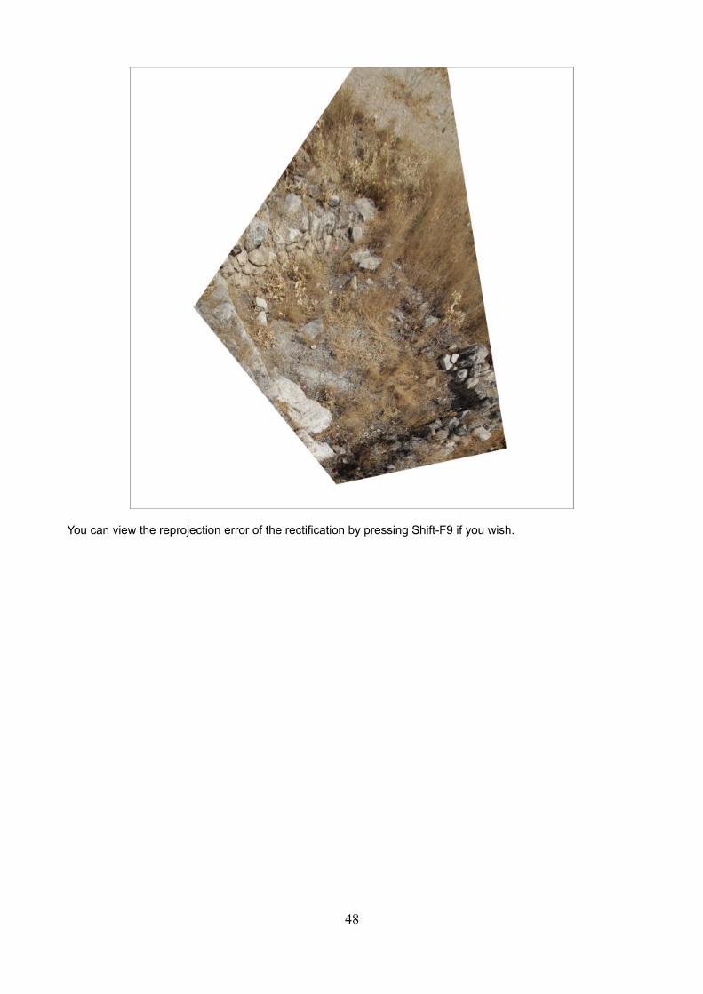
You can view the reprojection error of the rectification by pressing Shift-F9 if you wish.

48

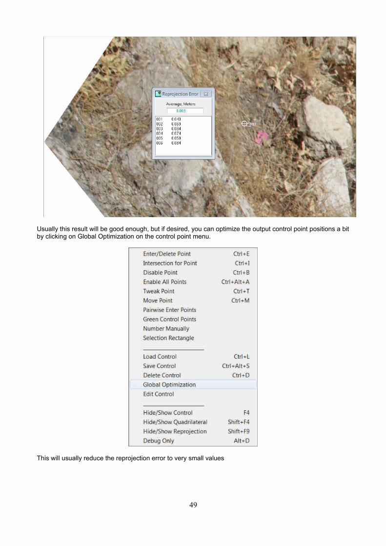
Usually this result will be good enough, but if desired, you can optimize the output control point positions a bitby clicking on Global Optimization on the control point menu.

This will usually reduce the reprojection error to very small values

49

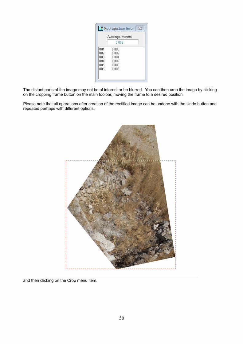
The distant parts of the image may not be of interest or be blurred. You can then crop the image by clicking on the cropping frame button on the main toolbar, moving the frame to a desired position

Please note that all operations after creation of the rectified image can be undone with the Undo button and repeated perhaps with different options.

and then clicking on the Crop menu item.

50

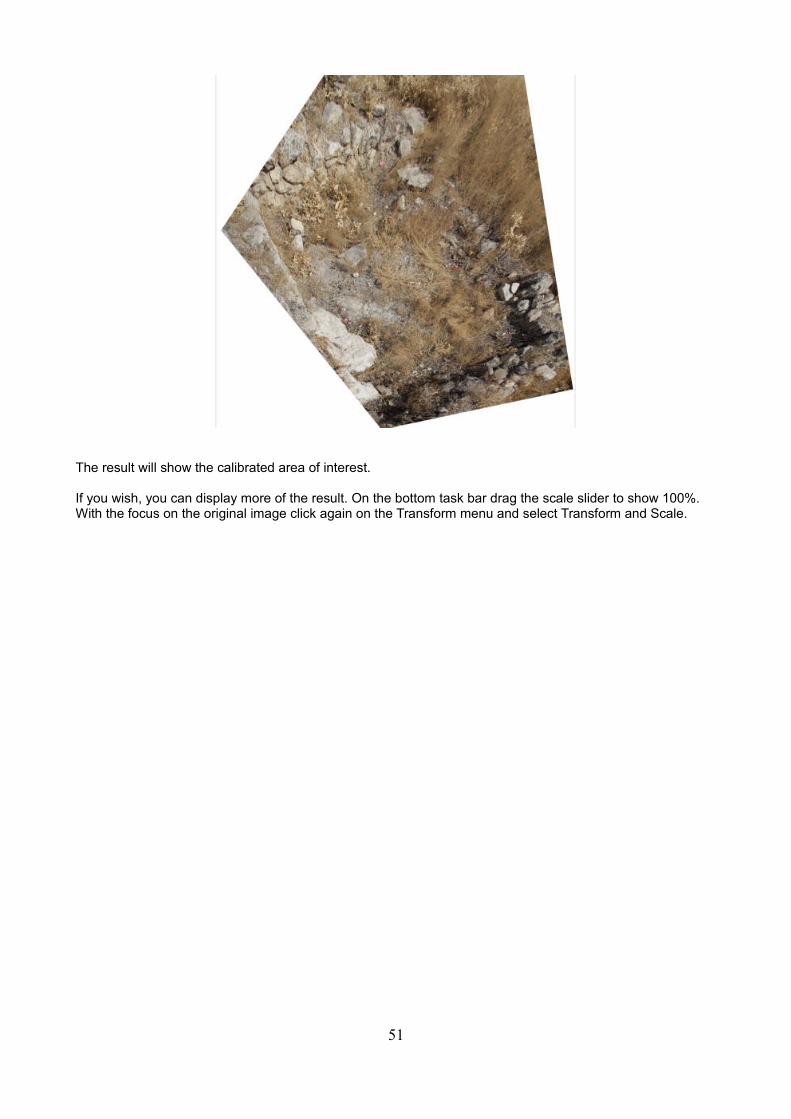
The result will show the calibrated area of interest.

If you wish, you can display more of the result. On the bottom task bar drag the scale slider to show 100%. With the focus on the original image click again on the Transform menu and select Transform and Scale.

51

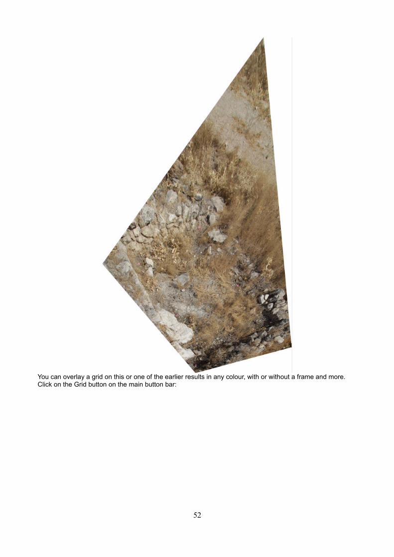
You can overlay a grid on this or one of the earlier results in any colour, with or without a frame and more. Click on the Grid button on the main button bar:

52

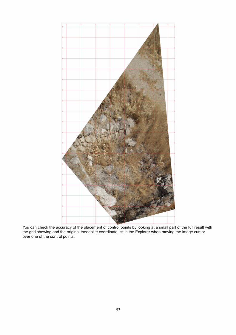
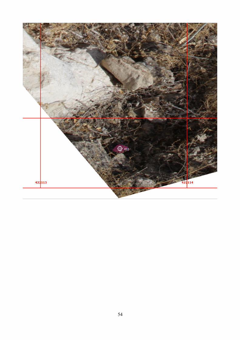
You can check the accuracy of the placement of control points by looking at a small part of the full result with the grid showing and the original theodolite coordinate list in the Explorer when moving the image cursor over one of the control points:

53

54

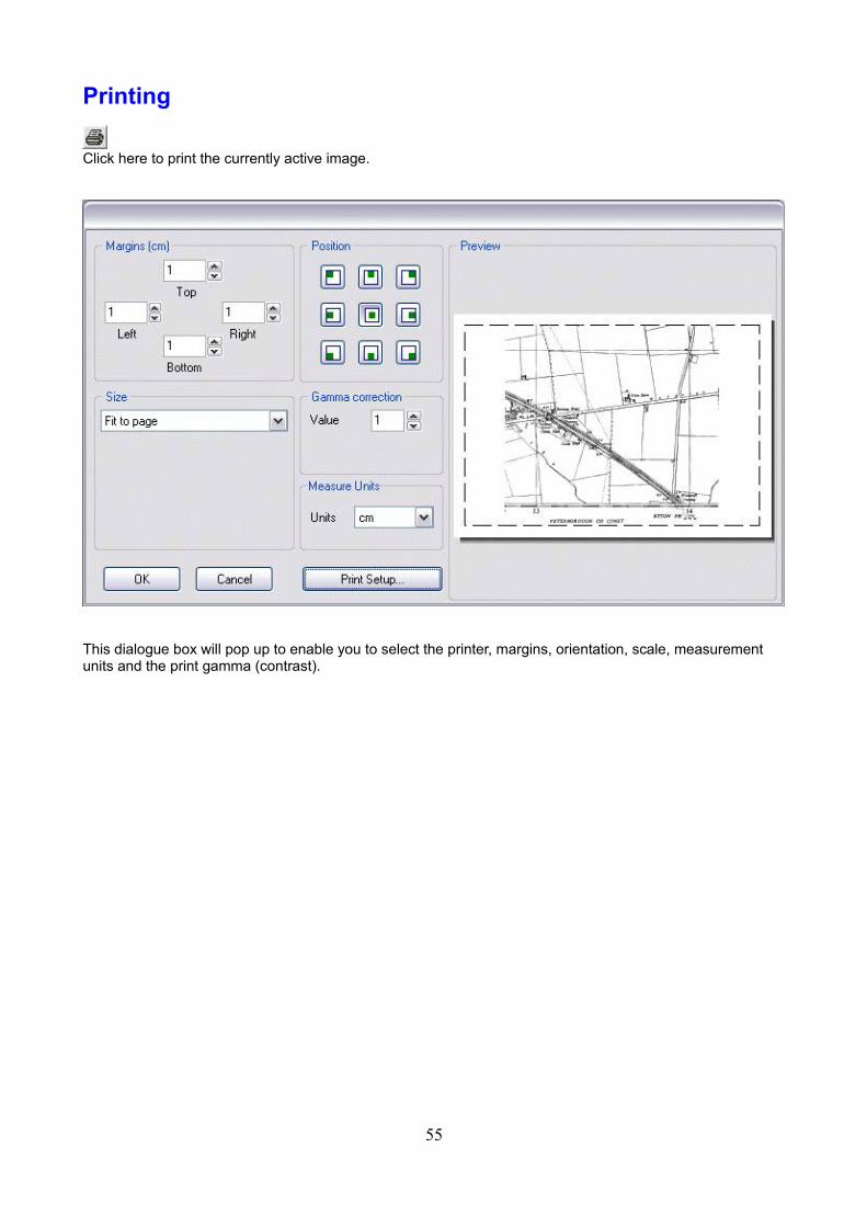
Printing

Click here to print the currently active image.

This dialogue box will pop up to enable you to select the printer, margins, orientation, scale, measurement units and the print gamma (contrast).

55

Options

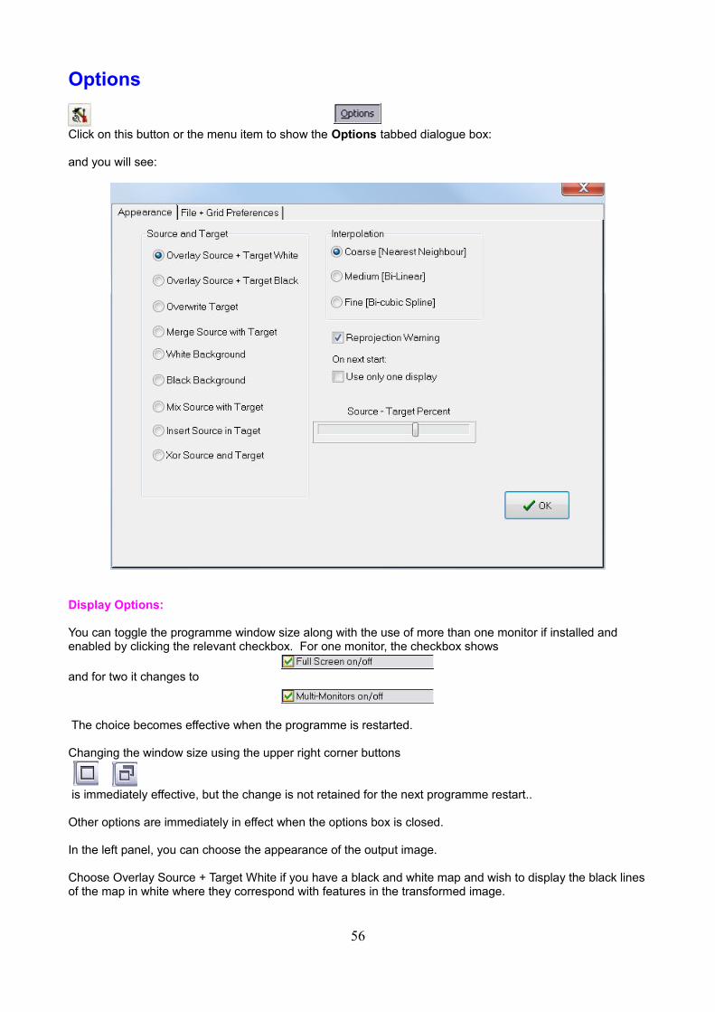
Click on this button or the menu item to show the Options tabbed dialogue box:

and you will see:

Display Options:

You can toggle the programme window size along with the use of more than one monitor if installed and enabled by clicking the relevant checkbox. For one monitor, the checkbox shows

and for two it changes to

The choice becomes effective when the programme is restarted.

Changing the window size using the upper right corner buttons

is immediately effective, but the change is not retained for the next programme restart..

Other options are immediately in effect when the options box is closed.

In the left panel, you can choose the appearance of the output image.

Choose Overlay Source + Target White if you have a black and white map and wish to display the black linesof the map in white where they correspond with features in the transformed image.

56

Choose Overlay Source + Target Black if you have a black and white map and wish to display the black lines of the map in black where they correspond with features in the transformed image.

Overwrite Target uses the input image (Source) to overwrite the output image (Target) after transformation regardless of the colour of the target.

Merge Source with Target places those parts of the input image in areas of the output image which are pure white, leaving the remainder of the output image untouched.

White and Black backgrounds create target images that show only the transformed data on the respective white or black backgrounds.

If you have chosen Mix as an output option, you can choose the percentage of mixture of the source and the target image after transformation with the track-bar next to the Mix button.

Inserting means that if a source image pixel is not white, it is inserted into the target, otherwise the target is left as it is.

The XOR option gives false colour output which may be useful for testing the visibility of a transformation to an image background like an othophoto. It is normally not used as a permanent result.

It is recommended to try various options followed by an Undo

to see what they do to your data. This must be done without using the Transform and scale option which does not support Undo, because it must close the original images before displaying them.

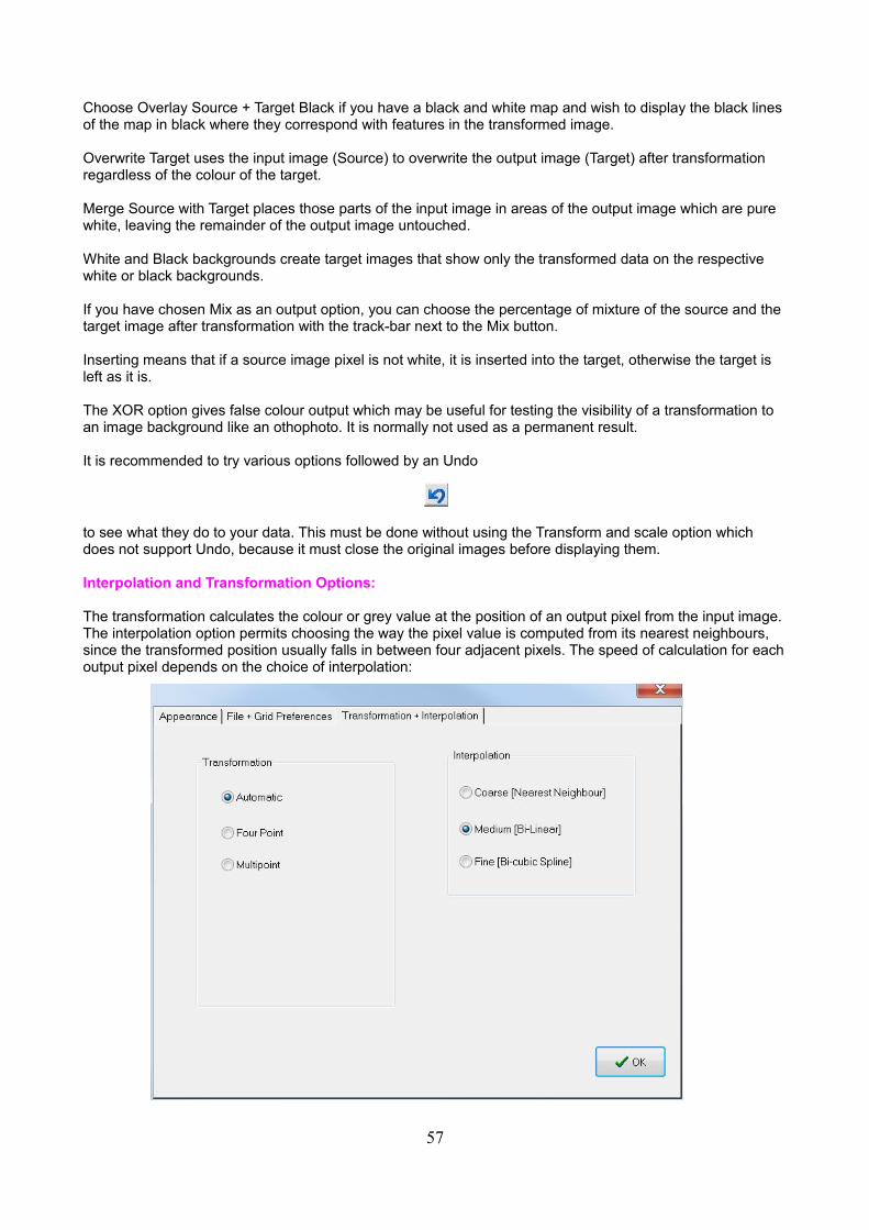
Interpolation and Transformation Options:

The transformation calculates the colour or grey value at the position of an output pixel from the input image. The interpolation option permits choosing the way the pixel value is computed from its nearest neighbours, since the transformed position usually falls in between four adjacent pixels. The speed of calculation for eachoutput pixel depends on the choice of interpolation:

57

Interpolation:

1) Coarse: the colour or grey value of the nearest neighbour to the computed input position is taken. This is the fastest method, but it may produce a jagged appearance in straight line features (aliasing).

2) Medium: the colour or grey value is interpolated bi-linearly dependent on the values of the four neighboursand the distance of the calculated point from them. This is nearly as fast as the nearest neighbour method, but it blurs the result slightly.

3) Fine: the colour or grey value is interpolated from the 16 nearest neighbours of the pixel using an approximation to a sin(x)/x (sinc) function which best preserves fine detail. Since considerably more calculation is required, this is the slowest method.

Transformation:

The programme computes an optimal transformation depending on the number of available control points in the source and target images. For 4 points, a projective transformation is computed. It does not take small errors in the positions of those points into account. For 5 or 6 points, a least-squares error fit is used. If there are 7 to 9 points, a second order non-linear correction is added to the least squares calculation. This compensates to some extent for radial lens distortion and moderate terrain height differences. For 10 to 12 points third order, 13-17 fourth order and 18 or more fifth order corrections are used which improve terrain matching and other smaller differences.

You can restrict calculation to a projective transformation only by choosing Projective, and only the least-squares error routines are used. If you have 7 or more points, you can force calculation to use the higher order corrections.

Reprojection Warning:

If you don't want to be bothered by warnings when the reprojection error exceeds 1% of the average side lengths of all images, uncheck the Reprojection Warning box.

File Default Options:

58

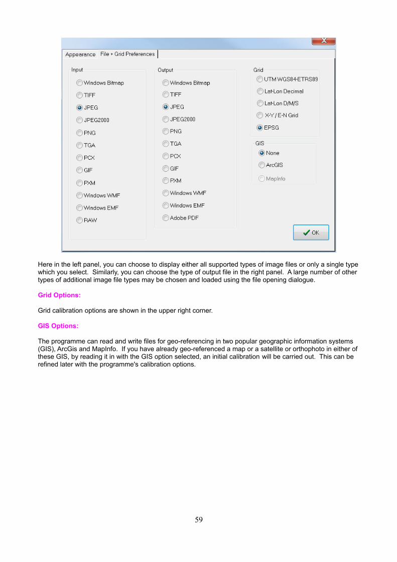
Here in the left panel, you can choose to display either all supported types of image files or only a single typewhich you select. Similarly, you can choose the type of output file in the right panel. A large number of other types of additional image file types may be chosen and loaded using the file opening dialogue.

Grid Options:

Grid calibration options are shown in the upper right corner.

GIS Options:

The programme can read and write files for geo-referencing in two popular geographic information systems (GIS), ArcGis and MapInfo. If you have already geo-referenced a map or a satellite or orthophoto in either ofthese GIS, by reading it in with the GIS option selected, an initial calibration will be carried out. This can be refined later with the programme's calibration options.

59

GeoPortal Data

Sources:

There are many hundreds of GeoPortal data servers which provide excellent maps and some of which provide orthophotos. Click on the links below to find an appropriate Geoportal in your area of interest.

A-F http://geographiccuriosities.freeservers.com/EurLinks1.htm

G-J http://geographiccuriosities.freeservers.com/EurLinks2.htm

I-R http://geographiccuriosities.freeservers.com/EurLinks3.htm

S-Z http://geographiccuriosities.freeservers.com/EurLinks4.htm4

Other sources of satellite, aerial images and maps:

Two general sources of satellite and aerial imagery and maps are Google's Maps and Microsoft's Bing Maps. The advanced version of Bing Maps is called Bing 3D, (formerly Virtual Earth). They are all in the GeoPortal list and may be used like any other URL in that list.

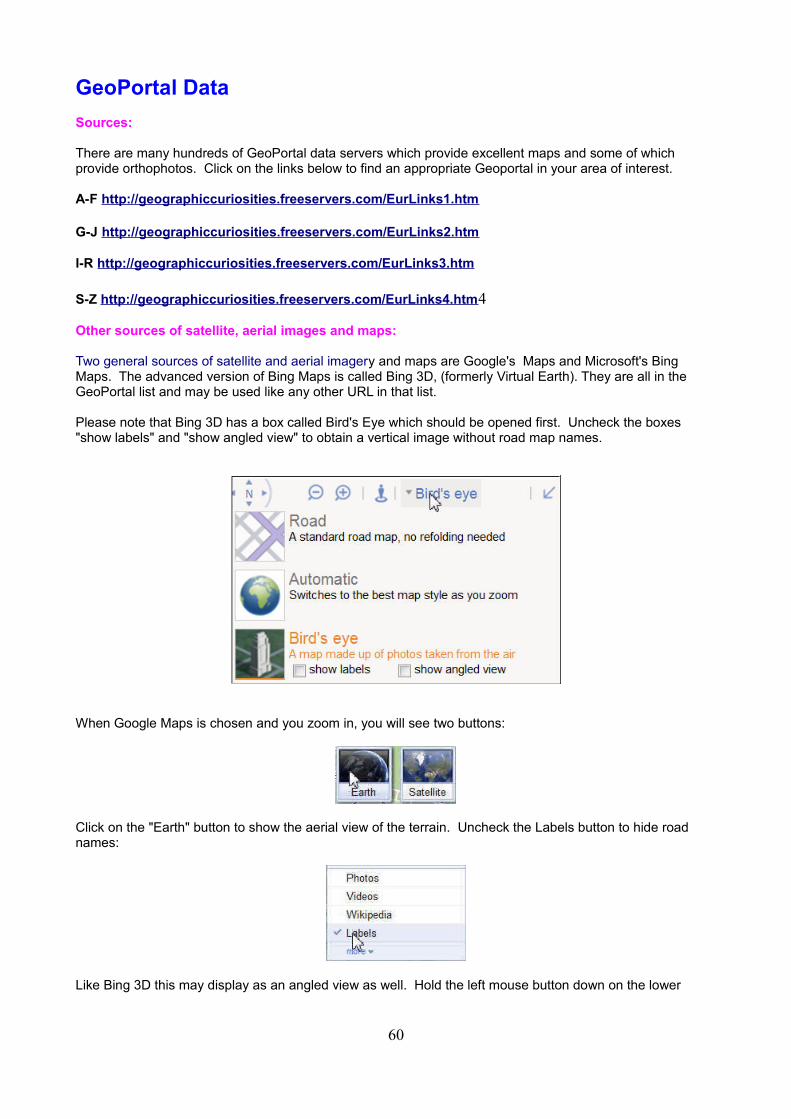
Please note that Bing 3D has a box called Bird's Eye which should be opened first. Uncheck the boxes "show labels" and "show angled view" to obtain a vertical image without road map names.

When Google Maps is chosen and you zoom in, you will see two buttons:

Click on the "Earth" button to show the aerial view of the terrain. Uncheck the Labels button to hide road names:

Like Bing 3D this may display as an angled view as well. Hold the left mouse button down on the lower

60

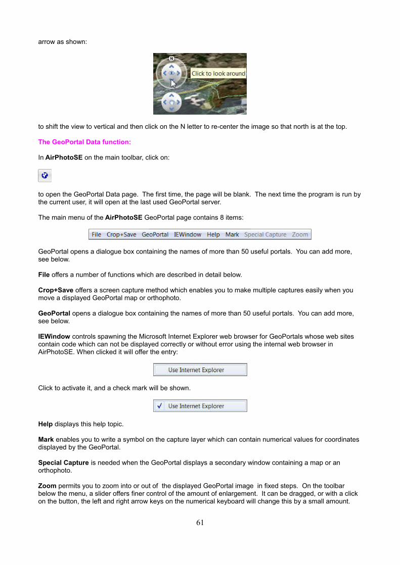
arrow as shown:

to shift the view to vertical and then click on the N letter to re-center the image so that north is at the top.

The GeoPortal Data function:

In AirPhotoSE on the main toolbar, click on:

to open the GeoPortal Data page. The first time, the page will be blank. The next time the program is run bythe current user, it will open at the last used GeoPortal server.

The main menu of the AirPhotoSE GeoPortal page contains 8 items:

GeoPortal opens a dialogue box containing the names of more than 50 useful portals. You can add more, see below.

File offers a number of functions which are described in detail below.

Crop+Save offers a screen capture method which enables you to make multiple captures easily when you move a displayed GeoPortal map or orthophoto.

GeoPortal opens a dialogue box containing the names of more than 50 useful portals. You can add more, see below.

IEWindow controls spawning the Microsoft Internet Explorer web browser for GeoPortals whose web sites contain code which can not be displayed correctly or without error using the internal web browser in AirPhotoSE. When clicked it will offer the entry:

Click to activate it, and a check mark will be shown.

Help displays this help topic.

Mark enables you to write a symbol on the capture layer which can contain numerical values for coordinates displayed by the GeoPortal.

Special Capture is needed when the GeoPortal displays a secondary window containing a map or an orthophoto.

Zoom permits you to zoom into or out of the displayed GeoPortal image in fixed steps. On the toolbar below the menu, a slider offers finer control of the amount of enlargement. It can be dragged, or with a click on the button, the left and right arrow keys on the numerical keyboard will change this by a small amount.

61

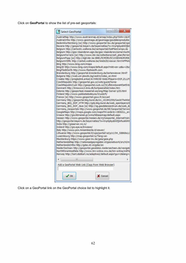
Click on GeoPortal to show the list of pre-set geoportals:

Click on a GeoPortal link on the GeoPortal choice list to highlight it.

62

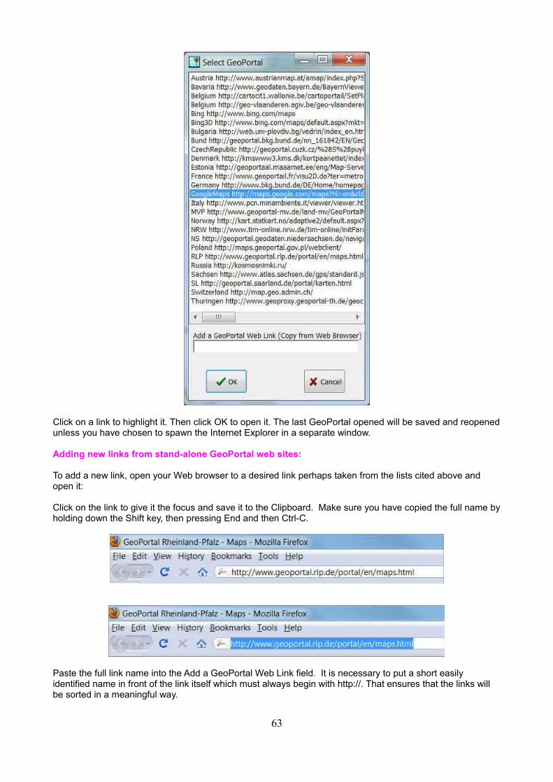
Click on a link to highlight it. Then click OK to open it. The last GeoPortal opened will be saved and reopenedunless you have chosen to spawn the Internet Explorer in a separate window.

Adding new links from stand-alone GeoPortal web sites:

To add a new link, open your Web browser to a desired link perhaps taken from the lists cited above and open it:

Click on the link to give it the focus and save it to the Clipboard. Make sure you have copied the full name byholding down the Shift key, then pressing End and then Ctrl-C.

Paste the full link name into the Add a GeoPortal Web Link field. It is necessary to put a short easily identified name in front of the link itself which must always begin with http://. That ensures that the links will be sorted in a meaningful way.

63

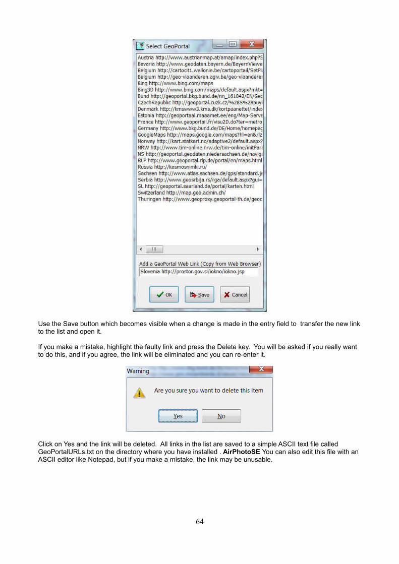
Use the Save button which becomes visible when a change is made in the entry field to transfer the new linkto the list and open it.

If you make a mistake, highlight the faulty link and press the Delete key. You will be asked if you really want to do this, and if you agree, the link will be eliminated and you can re-enter it.

Click on Yes and the link will be deleted. All links in the list are saved to a simple ASCII text file called GeoPortalURLs.txt on the directory where you have installed . AirPhotoSE You can also edit this file with an ASCII editor like Notepad, but if you make a mistake, the link may be unusable.

64

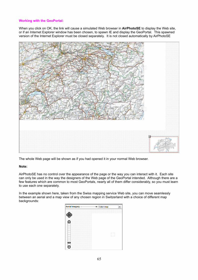
Working with the GeoPortal:

When you click on OK, the link will cause a simulated Web browser in AirPhotoSE to display the Web site, or if an Internet Explorer window has been chosen, to spawn IE and display the GeoPortal. This spawned version of the Internet Explorer must be closed separately. It is not closed automatically by AirPhotoSE

The whole Web page will be shown as if you had opened it in your normal Web browser.

Note:

AirPhotoSE has no control over the appearance of the page or the way you can interact with it. Each site can only be used in the way the designers of the Web page of the GeoPortal intended. Although there are a few features which are common to most GeoPortals, nearly all of them differ considerably, so you must learn to use each one separately.

In the example shown here, taken from the Swiss mapping service Web site, you can move seamlessly between an aerial and a map view of any chosen region in Switzerland with a choice of different mapbackgrounds:

65

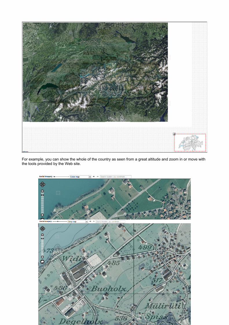
For example, you can show the whole of the country as seen from a great altitude and zoom in or move with the tools provided by the Web site.

66

On this site, you can display aerial and map detail with scales as large as 1:1000, but most other sites do notoffer such high resolution.

Well designed sites offer an option for mixing the aerial and the map view of an area and show grid lines in the coordinate system of the country. Many other items of interest can also be shown like in a GIS programme.

Warning:

For copyright or other reasons, many GeoPortal sites forbid doing anything except examining an area in their data window. Consult the conditions of use for a site of interest before using any of the options described in the following sections.

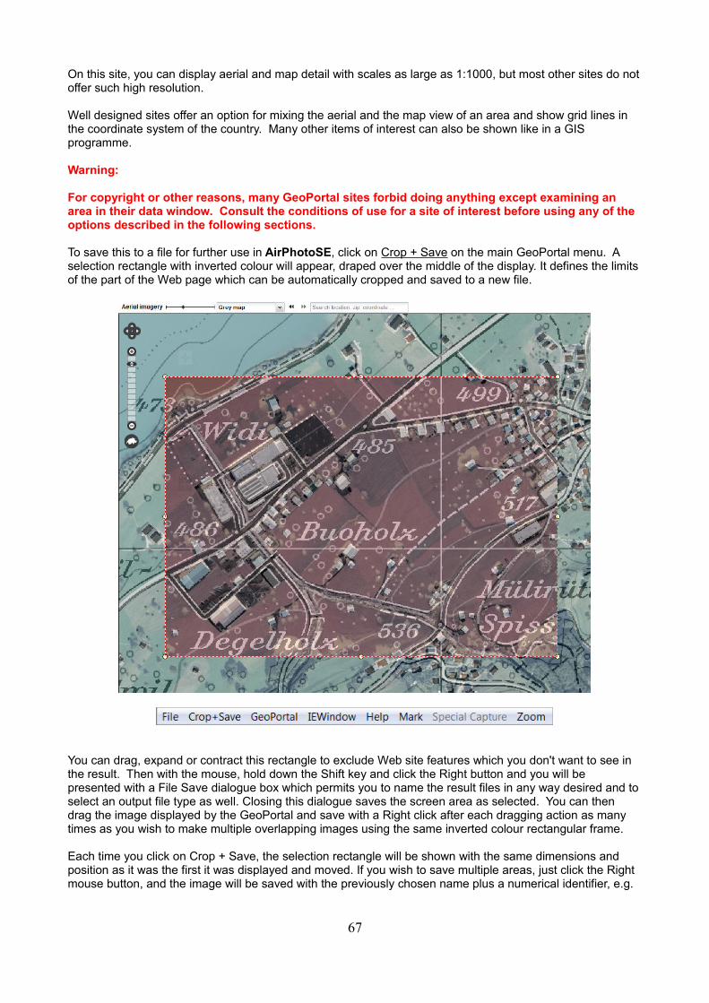
To save this to a file for further use in AirPhotoSE, click on Crop + Save on the main GeoPortal menu. A selection rectangle with inverted colour will appear, draped over the middle of the display. It defines the limitsof the part of the Web page which can be automatically cropped and saved to a new file.

You can drag, expand or contract this rectangle to exclude Web site features which you don't want to see in the result. Then with the mouse, hold down the Shift key and click the Right button and you will be presented with a File Save dialogue box which permits you to name the result files in any way desired and toselect an output file type as well. Closing this dialogue saves the screen area as selected. You can then drag the image displayed by the GeoPortal and save with a Right click after each dragging action as many times as you wish to make multiple overlapping images using the same inverted colour rectangular frame.

Each time you click on Crop + Save, the selection rectangle will be shown with the same dimensions and position as it was the first it was displayed and moved. If you wish to save multiple areas, just click the Right mouse button, and the image will be saved with the previously chosen name plus a numerical identifier, e.g.

67

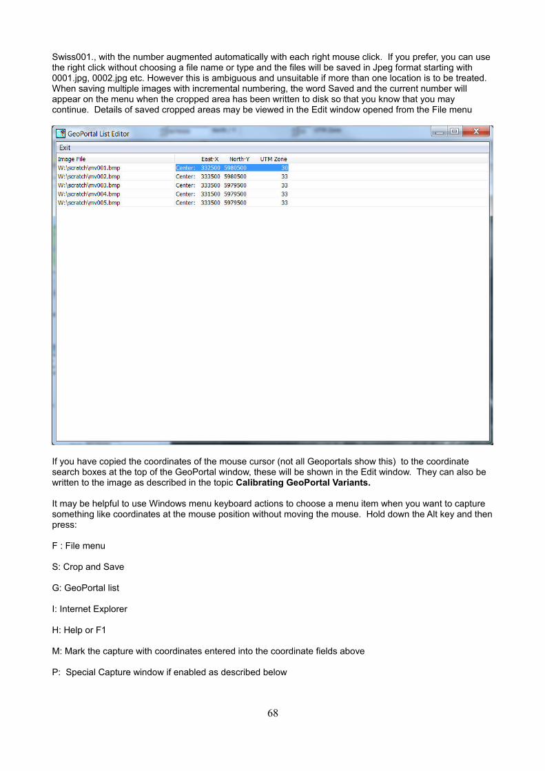
Swiss001., with the number augmented automatically with each right mouse click. If you prefer, you can use the right click without choosing a file name or type and the files will be saved in Jpeg format starting with 0001.jpg, 0002.jpg etc. However this is ambiguous and unsuitable if more than one location is to be treated. When saving multiple images with incremental numbering, the word Saved and the current number will appear on the menu when the cropped area has been written to disk so that you know that you may continue. Details of saved cropped areas may be viewed in the Edit window opened from the File menu

If you have copied the coordinates of the mouse cursor (not all Geoportals show this) to the coordinate search boxes at the top of the GeoPortal window, these will be shown in the Edit window. They can also be written to the image as described in the topic Calibrating GeoPortal Variants.

It may be helpful to use Windows menu keyboard actions to choose a menu item when you want to capture something like coordinates at the mouse position without moving the mouse. Hold down the Alt key and thenpress:

F : File menu

S: Crop and Save

G: GeoPortal list

I: Internet Explorer

H: Help or F1

M: Mark the capture with coordinates entered into the coordinate fields above

P: Special Capture window if enabled as described below

68

Z: Zoom

This will allow you to change layers in GeoPortal, and crop a matching area of map and photo precisely in separate files. The quality of the match between the aerial or satellite image and the map will vary, depending on their relative original scales. If these differ considerably, then items like buildings or roads maybe displaced considerably.

Note:

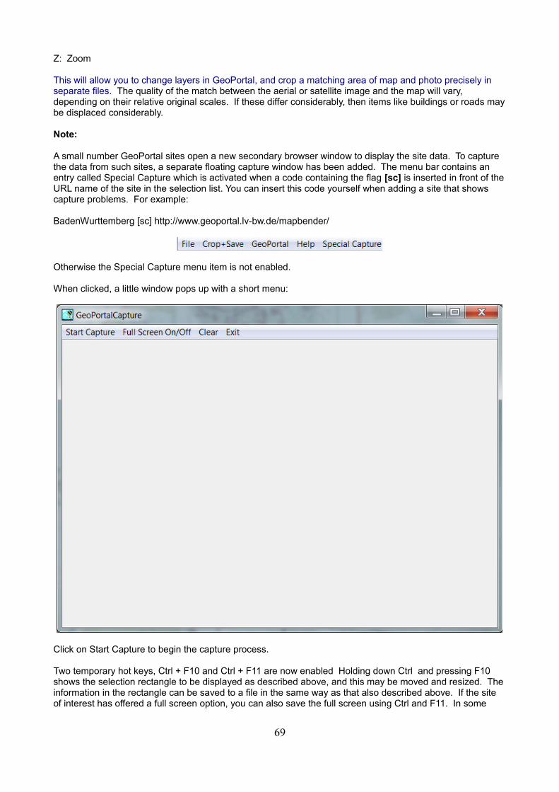
A small number GeoPortal sites open a new secondary browser window to display the site data. To capture the data from such sites, a separate floating capture window has been added. The menu bar contains an entry called Special Capture which is activated when a code containing the flag [sc] is inserted in front of theURL name of the site in the selection list. You can insert this code yourself when adding a site that shows capture problems. For example:

BadenWurttemberg [sc] http://www.geoportal.lv-bw.de/mapbender/

Otherwise the Special Capture menu item is not enabled.

When clicked, a little window pops up with a short menu:

Click on Start Capture to begin the capture process.

Two temporary hot keys, Ctrl + F10 and Ctrl + F11 are now enabled Holding down Ctrl and pressing F10 shows the selection rectangle to be displayed as described above, and this may be moved and resized. Theinformation in the rectangle can be saved to a file in the same way as that also described above. If the site of interest has offered a full screen option, you can also save the full screen using Ctrl and F11. In some

69

cases, other programmes may be using the Ctrl and F11 combination. In that case a message will inform you that the capture window will try to use Ctrl and F9.

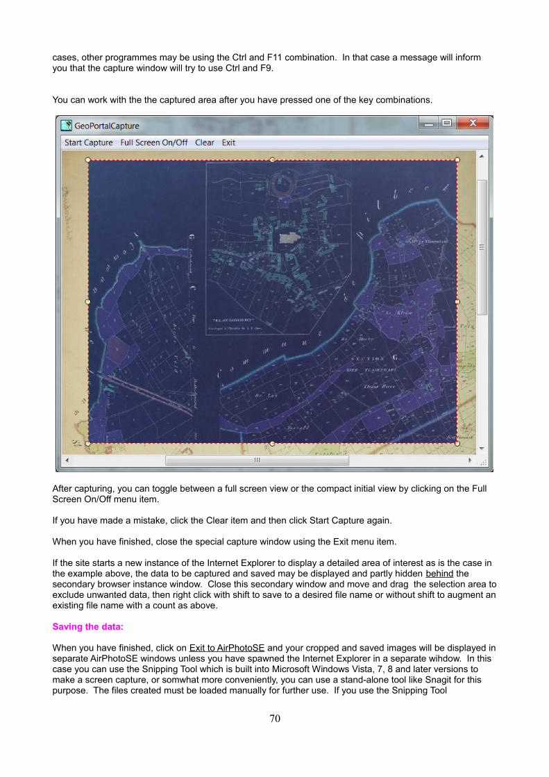
You can work with the the captured area after you have pressed one of the key combinations.

After capturing, you can toggle between a full screen view or the compact initial view by clicking on the Full Screen On/Off menu item.

If you have made a mistake, click the Clear item and then click Start Capture again.

When you have finished, close the special capture window using the Exit menu item.

If the site starts a new instance of the Internet Explorer to display a detailed area of interest as is the case in the example above, the data to be captured and saved may be displayed and partly hidden behind the secondary browser instance window. Close this secondary window and move and drag the selection area toexclude unwanted data, then right click with shift to save to a desired file name or without shift to augment anexisting file name with a count as above.

Saving the data:

When you have finished, click on Exit to AirPhotoSE and your cropped and saved images will be displayed inseparate AirPhotoSE windows unless you have spawned the Internet Explorer in a separate wihdow. In this case you can use the Snipping Tool which is built into Microsoft Windows Vista, 7, 8 and later versions to make a screen capture, or somwhat more conveniently, you can use a stand-alone tool like Snagit for this purpose. The files created must be loaded manually for further use. If you use the Snipping Tool

70

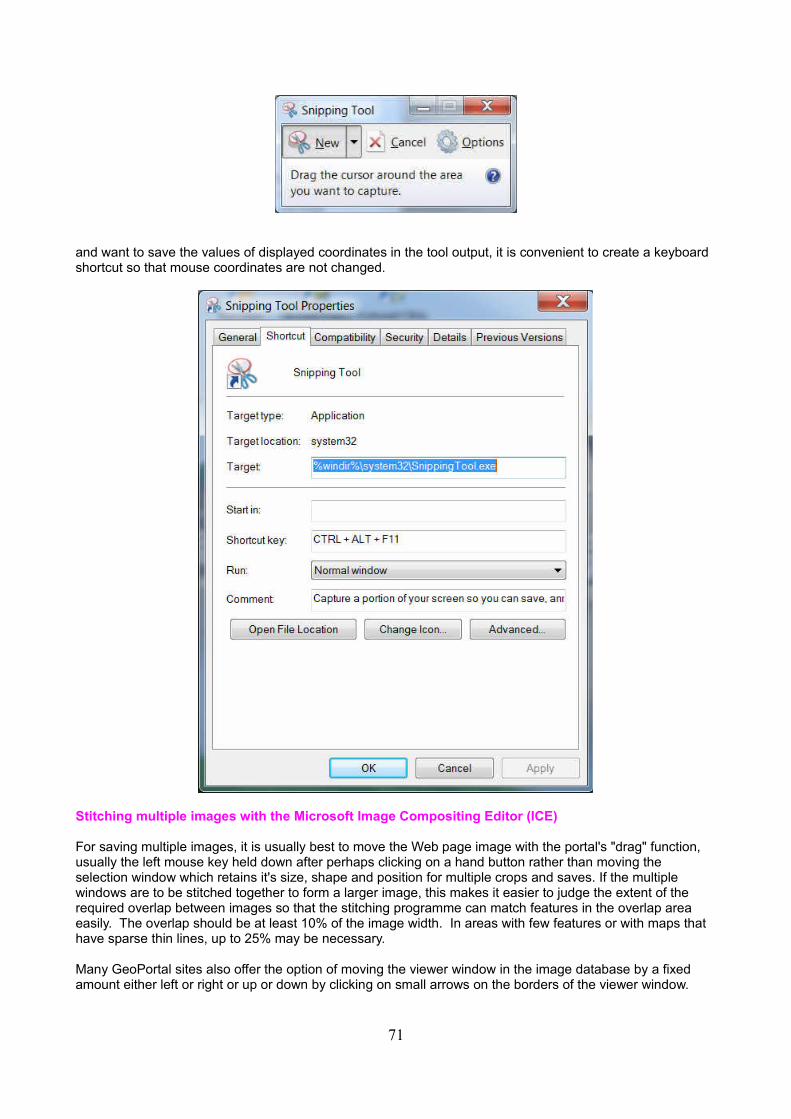
and want to save the values of displayed coordinates in the tool output, it is convenient to create a keyboard shortcut so that mouse coordinates are not changed.

Stitching multiple images with the Microsoft Image Compositing Editor (ICE)

For saving multiple images, it is usually best to move the Web page image with the portal's "drag" function, usually the left mouse key held down after perhaps clicking on a hand button rather than moving the selection window which retains it's size, shape and position for multiple crops and saves. If the multiple windows are to be stitched together to form a larger image, this makes it easier to judge the extent of the required overlap between images so that the stitching programme can match features in the overlap area easily. The overlap should be at least 10% of the image width. In areas with few features or with maps that have sparse thin lines, up to 25% may be necessary.

Many GeoPortal sites also offer the option of moving the viewer window in the image database by a fixed amount either left or right or up or down by clicking on small arrows on the borders of the viewer window.

71

This makes it easy to keep multiple images aligned.If calibration of the result is desired, and if the GeoPortal offers a search option using numerical coordinates in a local grid or in UTM, then it is helpful to move in fixed distance steps to the east or west and north or south such that the saved image tiles overlap. Some GeoPortal sites place a marker at the centre of the image after moving. The coordinates entered in the search option can usually be saved to the Clipboard andpasted into Notepad running at the same time to create a list of centre coordinates for each tile. These may then be used as calibration points.

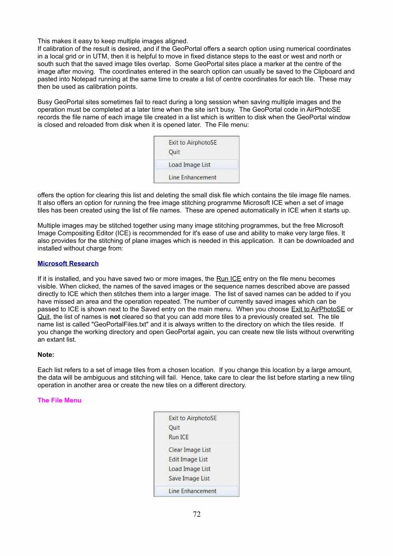
Busy GeoPortal sites sometimes fail to react during a long session when saving multiple images and the operation must be completed at a later time when the site isn't busy. The GeoPortal code in AirPhotoSE records the file name of each image tile created in a list which is written to disk when the GeoPortal window is closed and reloaded from disk when it is opened later. The File menu:

offers the option for clearing this list and deleting the small disk file which contains the tile image file names. It also offers an option for running the free image stitching programme Microsoft ICE when a set of image tiles has been created using the list of file names. These are opened automatically in ICE when it starts up.

Multiple images may be stitched together using many image stitching programmes, but the free Microsoft Image Compositing Editor (ICE) is recommended for it's ease of use and ability to make very large files. It also provides for the stitching of plane images which is needed in this application. It can be downloaded andinstalled without charge from:

Microsoft Research

If it is installed, and you have saved two or more images, the Run ICE entry on the file menu becomes visible. When clicked, the names of the saved images or the sequence names described above are passed directly to ICE which then stitches them into a larger image. The list of saved names can be added to if you have missed an area and the operation repeated. The number of currently saved images which can be passed to ICE is shown next to the Saved entry on the main menu. When you choose Exit to AirPhotoSE or Quit, the list of names is not cleared so that you can add more tiles to a previously created set. The tile name list is called "GeoPortalFiles.txt" and it is always written to the directory on which the tiles reside. If you change the working directory and open GeoPortal again, you can create new tile lists without overwritingan extant list.

Note:

Each list refers to a set of image tiles from a chosen location. If you change this location by a large amount, the data will be ambiguous and stitching will fail. Hence, take care to clear the list before starting a new tilingoperation in another area or create the new tiles on a different directory.

The File Menu

72

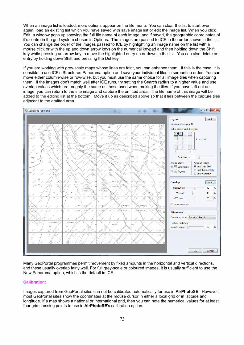
When an image list is loaded, more options appear on the file menu. You can clear the list to start over again, load an existing list which you have saved with save image list or edit the image list. When you click Edit, a window pops up showing the full file name of each image, and if saved, the geographic coordinates ofit's centre in the grid system chosen in Options. The images are passed to ICE in the order shown in the list.You can change the order of the images passed to ICE by highlighting an image name on the list with a mouse click or with the up and down arrow keys on the numerical keypad and then holding down the Shift key while pressing an arrow key to move the highlighted entry up or down in the list. You can also delete an entry by holding down Shift and pressing the Del key.

If you are working with grey-scale maps whose lines are faint, you can enhance them. If this is the case, it issensible to use ICE's Structured Panorama option and save your individual tiles in serpentine order. You canmove either column-wise or row-wise, but you must use the same choice for all image tiles when capturing them. If the images don't match well after ICE runs, try setting the Search radius to a higher value and use overlap values which are roughly the same as those used when making the tiles. If you have left out an image, you can return to the site image and capture the omitted area. The file name of this image will be added to the editing list at the bottom, Move it up as described above so that it lies between the capture tilesadjacent to the omitted area.

Many GeoPortal programmes permit movement by fixed amounts in the horizontal and vertical directions, and these usually overlap fairly well. For full grey-scale or coloured images, it is usually sufficient to use the New Panorama option, which is the default in ICE.

Calibration:

Images captured from GeoPortal sites can not be calibrated automatically for use in AirPhotoSE. However, most GeoPortal sites show the coordinates at the mouse cursor in either a local grid or in latitude and longitude. If a map shows a national or international grid, then you can note the numerical values for at least four grid crossing points to use in AirPhotoSE's calibration option.

73

If no grid is shown, you can note the coordinates of prominent features which you will be able to see easily when the images have been saved and displayed in AirPhotoSE. Google Maps for example, shows the latitude and longitude at any point with a right click and places this into it's Search field. From there it can becopied to the clipboard. If you have opened Notebook before opening GeoPortal, you can paste this value along with those of other easily recognized points into the Notebook page from which they can then be pasted into the AirPhotoSE calibration dialogue box.

Special Sites:

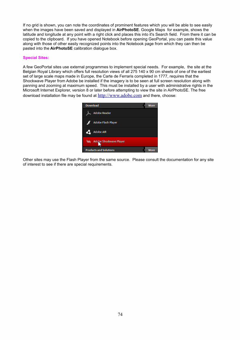
A few GeoPortal sites use external programmes to implement special needs. For example, the site at the Belgian Royal Library which offers full resolution views of all 275 140 x 90 cm sheets of one of the earliest set of large scale maps made in Europe, the Carte de Ferraris completed in 1777, requires that the Shockwave Player from Adobe be installed if the imagery is to be seen at full screen resolution along with panning and zooming at maximum speed. This must be installed by a user with administrative rights in the Microsoft Internet Explorer, version 8 or later before attempting to view the site in AirPhotoSE. The free download installation file may be found at http://www.adobe.com and there, choose:

Other sites may use the Flash Player from the same source. Please consult the documentation for any site of interest to see if there are special requirements.

74

Calibration of maps and orthophotos

What is calibration?

Large scale maps which can be used for accurately locating the features visible in an aerial photograph are remade at intervals, and their geographic grids have been revised over time by the map makers. Data from satellite or aerial image servers are revised even more frequently. Positional data determined by geodesy is more or less forever in terms of human life span, whereas field boundaries seen from the air change yearly interms of the way they look and so-called fixed points visible in an aerial photograph can vanish at the flick of a lever on a bulldozer. Geodesy, meaning the accurate measurement of the shape of the Earth, used to be determined by astronomy, and now it's determined by accurate GPS measurement. Field boundaries are determined by agricultural requirements, land prices and the needs of farmers etc. and should never be considered as fixed.

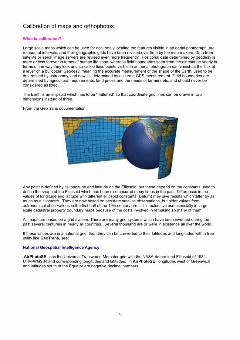
The Earth is an ellipsoid which has to be "flattened" so that coordinate grid lines can be drawn in two dimensions instead of three.

From the GeoTrans documentation:

Any point is defined by its longitude and latitude on the Ellipsoid, but these depend on the constants used to define the shape of the Ellipsoid which has been re-measured many times in the past. Differences in the values of longitude and latitude with different ellipsoid constants (Datum) may give results which differ by as much as a kilometre. They are now based on accurate satellite observations, but older values from astronomical observations in the first half of the 19th century are still in extensive use especially in large scale cadastral property boundary maps because of the costs involved in remaking so many of them.

All maps are based on a grid system. There are many grid systems which have been invented during the past several centuries in nearly all countries. Several thousand are or were in existence all over the world.

If these values are in a national grid, then they can be converted to their latitudes and longitudes with a free utility like GeoTrans, see:

National Geospatial Intelligence Agency

AirPhotoSE uses the Universal Transverse Mercator grid with the NASA-determined Ellipsoid of 1984, UTM-WGS84 and corresponding longitudes and latitudes. In AirPhotoSE, longitudes west of Greenwich and latitudes south of the Equator are negative decimal numbers.

75

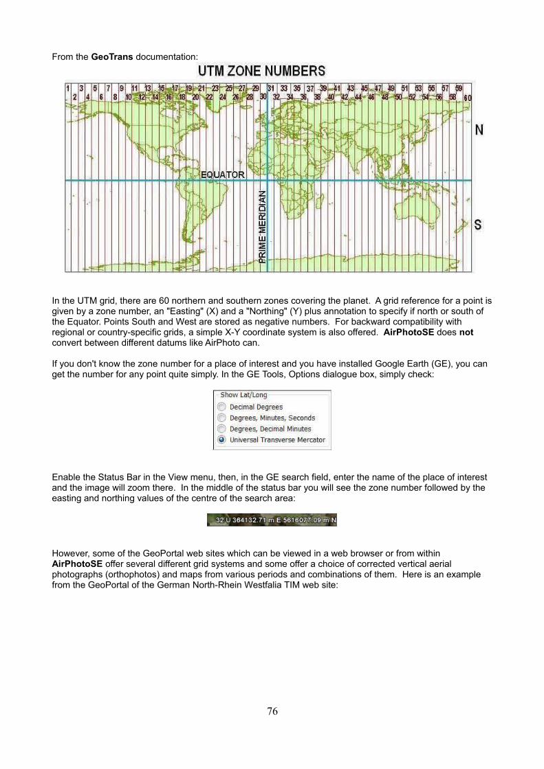
From the GeoTrans documentation:

In the UTM grid, there are 60 northern and southern zones covering the planet. A grid reference for a point isgiven by a zone number, an "Easting" (X) and a "Northing" (Y) plus annotation to specify if north or south of the Equator. Points South and West are stored as negative numbers. For backward compatibility with regional or country-specific grids, a simple X-Y coordinate system is also offered. AirPhotoSE does not convert between different datums like AirPhoto can.

If you don't know the zone number for a place of interest and you have installed Google Earth (GE), you can get the number for any point quite simply. In the GE Tools, Options dialogue box, simply check:

Enable the Status Bar in the View menu, then, in the GE search field, enter the name of the place of interest and the image will zoom there. In the middle of the status bar you will see the zone number followed by the easting and northing values of the centre of the search area:

However, some of the GeoPortal web sites which can be viewed in a web browser or from within AirPhotoSE offer several different grid systems and some offer a choice of corrected vertical aerial photographs (orthophotos) and maps from various periods and combinations of them. Here is an example from the GeoPortal of the German North-Rhein Westfalia TIM web site:

76

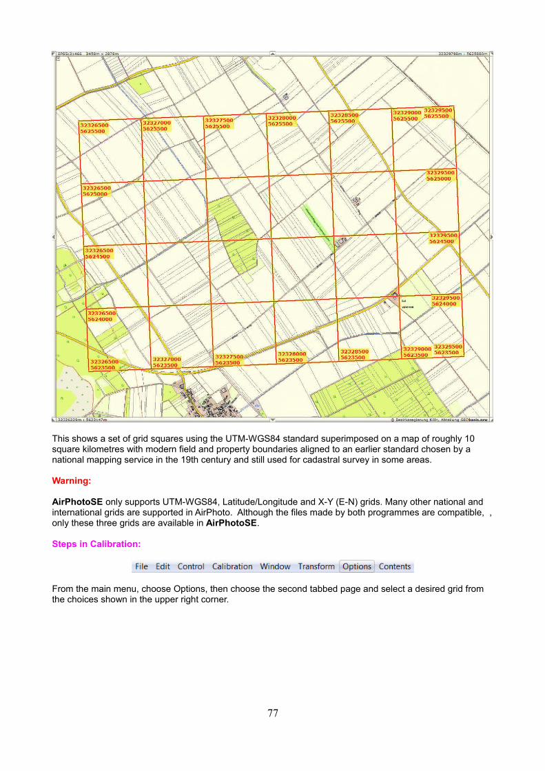
This shows a set of grid squares using the UTM-WGS84 standard superimposed on a map of roughly 10 square kilometres with modern field and property boundaries aligned to an earlier standard chosen by a national mapping service in the 19th century and still used for cadastral survey in some areas.

Warning:

AirPhotoSE only supports UTM-WGS84, Latitude/Longitude and X-Y (E-N) grids. Many other national and international grids are supported in AirPhoto. Although the files made by both programmes are compatible, ,only these three grids are available in AirPhotoSE.

Steps in Calibration:

From the main menu, choose Options, then choose the second tabbed page and select a desired grid from the choices shown in the upper right corner.

77

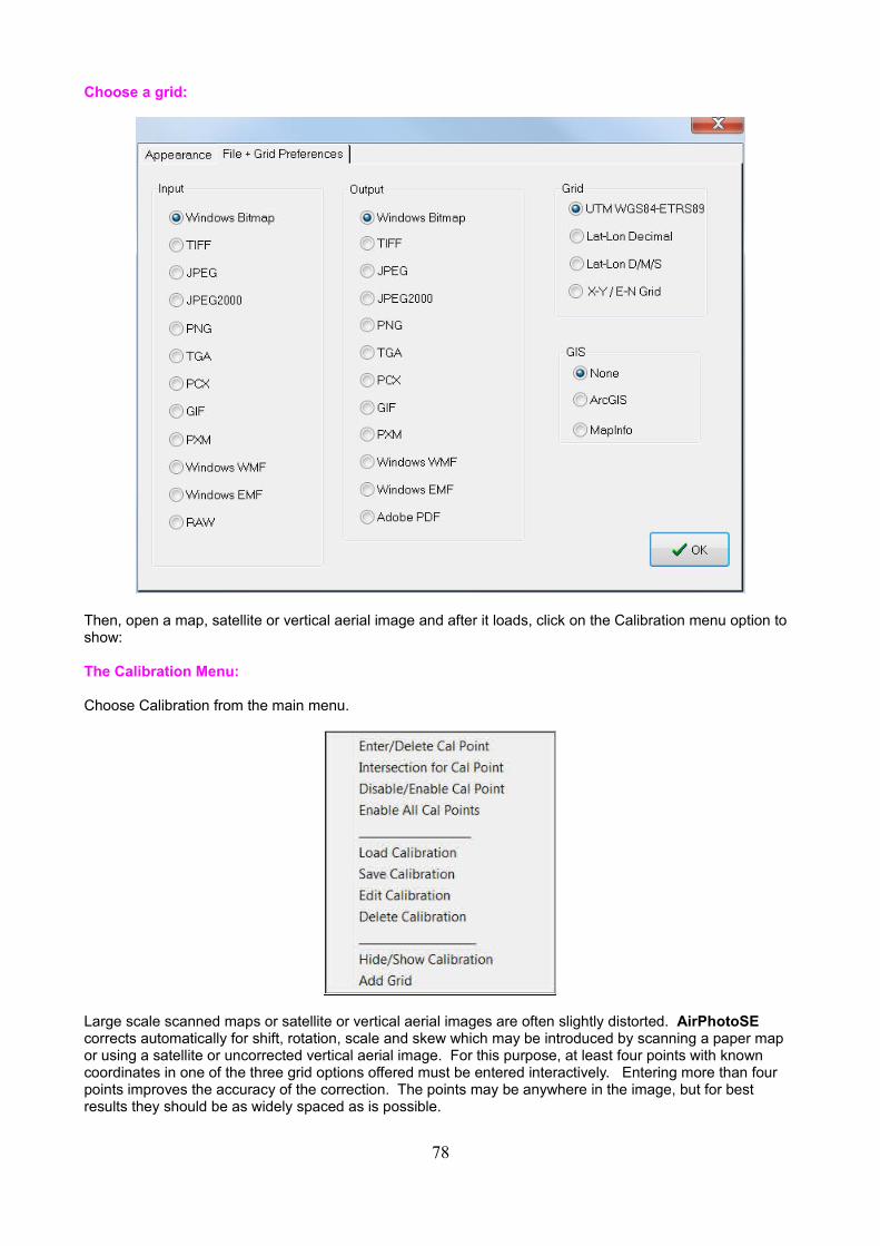
Choose a grid:

Then, open a map, satellite or vertical aerial image and after it loads, click on the Calibration menu option to show:

The Calibration Menu:

Choose Calibration from the main menu.

Large scale scanned maps or satellite or vertical aerial images are often slightly distorted. AirPhotoSE corrects automatically for shift, rotation, scale and skew which may be introduced by scanning a paper map or using a satellite or uncorrected vertical aerial image. For this purpose, at least four points with known coordinates in one of the three grid options offered must be entered interactively. Entering more than four points improves the accuracy of the correction. The points may be anywhere in the image, but for best results they should be as widely spaced as is possible.

78

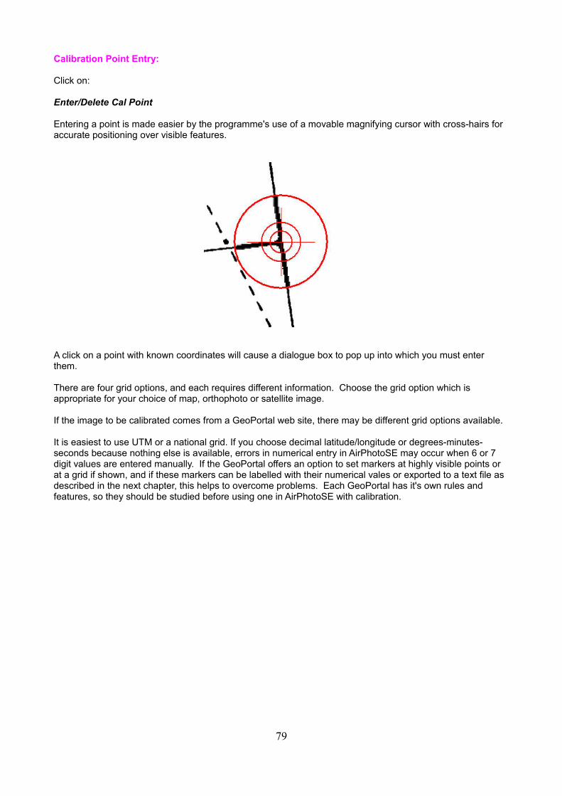
Calibration Point Entry:

Click on:

Enter/Delete Cal Point

Entering a point is made easier by the programme's use of a movable magnifying cursor with cross-hairs for accurate positioning over visible features.

A click on a point with known coordinates will cause a dialogue box to pop up into which you must enter them.

There are four grid options, and each requires different information. Choose the grid option which is appropriate for your choice of map, orthophoto or satellite image.

If the image to be calibrated comes from a GeoPortal web site, there may be different grid options available.

It is easiest to use UTM or a national grid. If you choose decimal latitude/longitude or degrees-minutes-seconds because nothing else is available, errors in numerical entry in AirPhotoSE may occur when 6 or 7 digit values are entered manually. If the GeoPortal offers an option to set markers at highly visible points or at a grid if shown, and if these markers can be labelled with their numerical vales or exported to a text file as described in the next chapter, this helps to overcome problems. Each GeoPortal has it's own rules and features, so they should be studied before using one in AirPhotoSE with calibration.

79

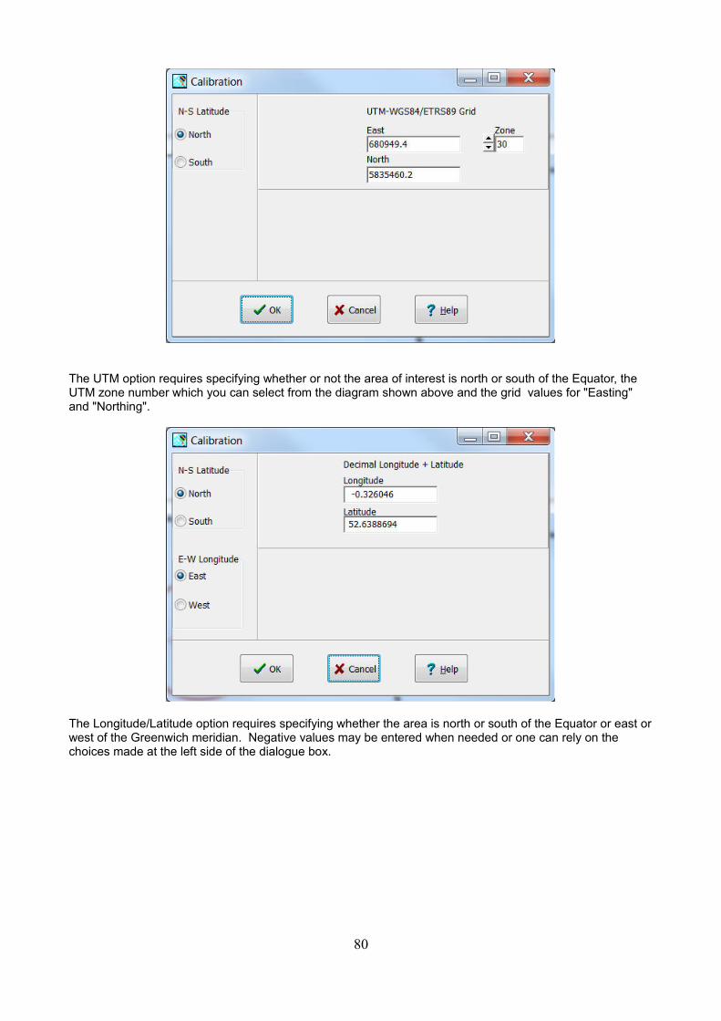
The UTM option requires specifying whether or not the area of interest is north or south of the Equator, the UTM zone number which you can select from the diagram shown above and the grid values for "Easting" and "Northing".

The Longitude/Latitude option requires specifying whether the area is north or south of the Equator or east orwest of the Greenwich meridian. Negative values may be entered when needed or one can rely on the choices made at the left side of the dialogue box.

80

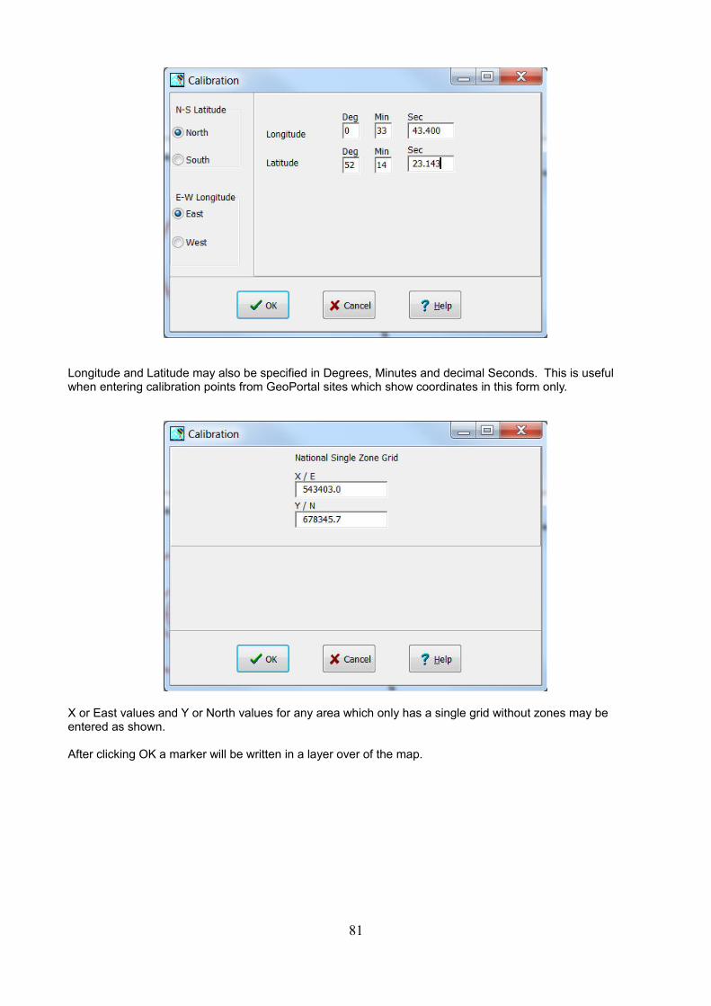
Longitude and Latitude may also be specified in Degrees, Minutes and decimal Seconds. This is useful when entering calibration points from GeoPortal sites which show coordinates in this form only.

X or East values and Y or North values for any area which only has a single grid without zones may be entered as shown.

After clicking OK a marker will be written in a layer over of the map.

81

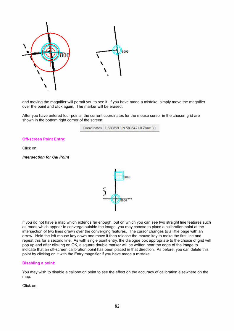
and moving the magnifier will permit you to see it. If you have made a mistake, simply move the magnifier over the point and click again. The marker will be erased.

After you have entered four points, the current coordinates for the mouse cursor in the chosen grid are shown in the bottom right corner of the screen:

Off-screen Point Entry:

Click on:

Intersection for Cal Point

If you do not have a map which extends far enough, but on which you can see two straight line features suchas roads which appear to converge outside the image, you may choose to place a calibration point at the intersection of two lines drawn over the converging features. The cursor changes to a little page with an arrow. Hold the left mouse key down and move it then release the mouse key to make the first line and repeat this for a second line. As with single point entry, the dialogue box appropriate to the choice of grid willpop up and after clicking on OK, a square double marker will be written near the edge of the image to indicate that an off-screen calibration point has been placed in that direction. As before, you can delete this point by clicking on it with the Entry magnifier if you have made a mistake.

Disabling a point:

You may wish to disable a calibration point to see the effect on the accuracy of calibration elsewhere on the map.

Click on:

82

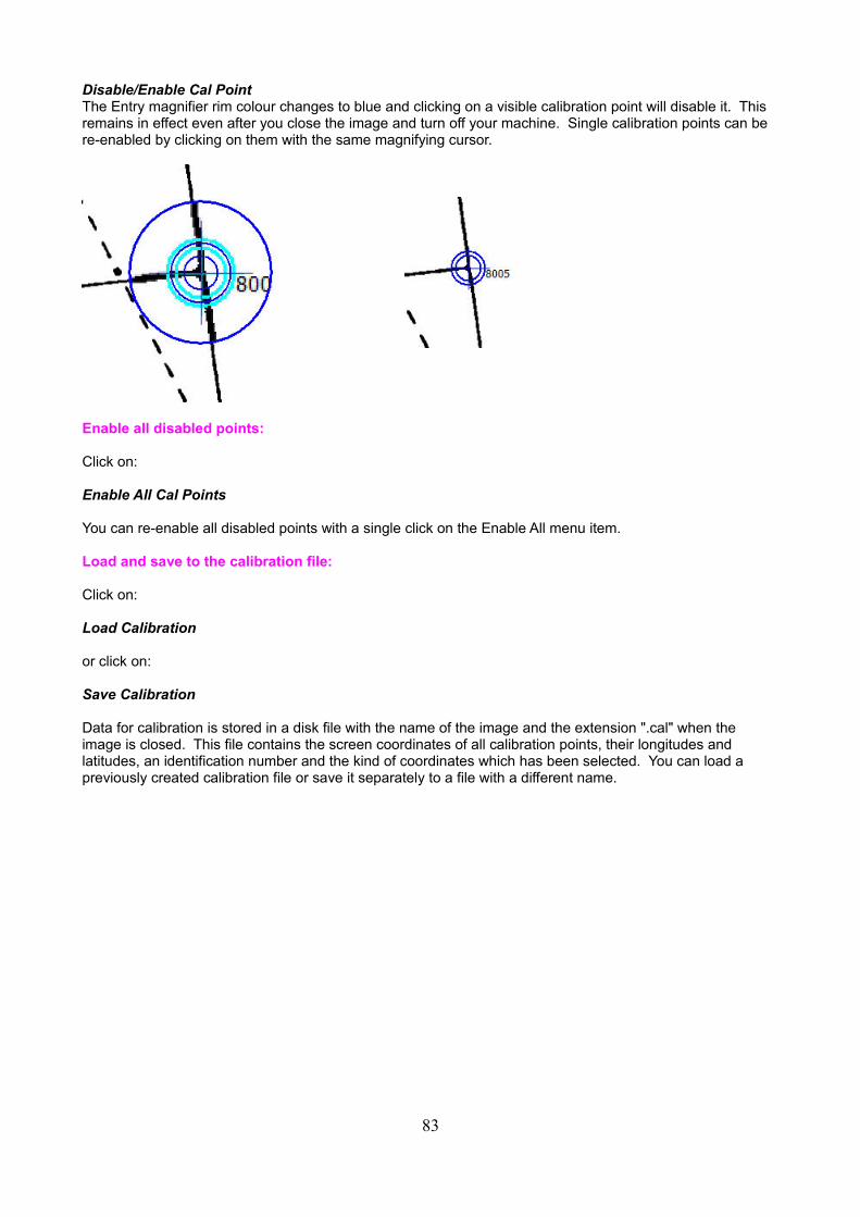
Disable/Enable Cal PointThe Entry magnifier rim colour changes to blue and clicking on a visible calibration point will disable it. This remains in effect even after you close the image and turn off your machine. Single calibration points can be re-enabled by clicking on them with the same magnifying cursor.

Enable all disabled points:

Click on:

Enable All Cal Points

You can re-enable all disabled points with a single click on the Enable All menu item.

Load and save to the calibration file:

Click on:

Load Calibration

or click on:

Save Calibration

Data for calibration is stored in a disk file with the name of the image and the extension ".cal" when the image is closed. This file contains the screen coordinates of all calibration points, their longitudes and latitudes, an identification number and the kind of coordinates which has been selected. You can load a previously created calibration file or save it separately to a file with a different name.

83

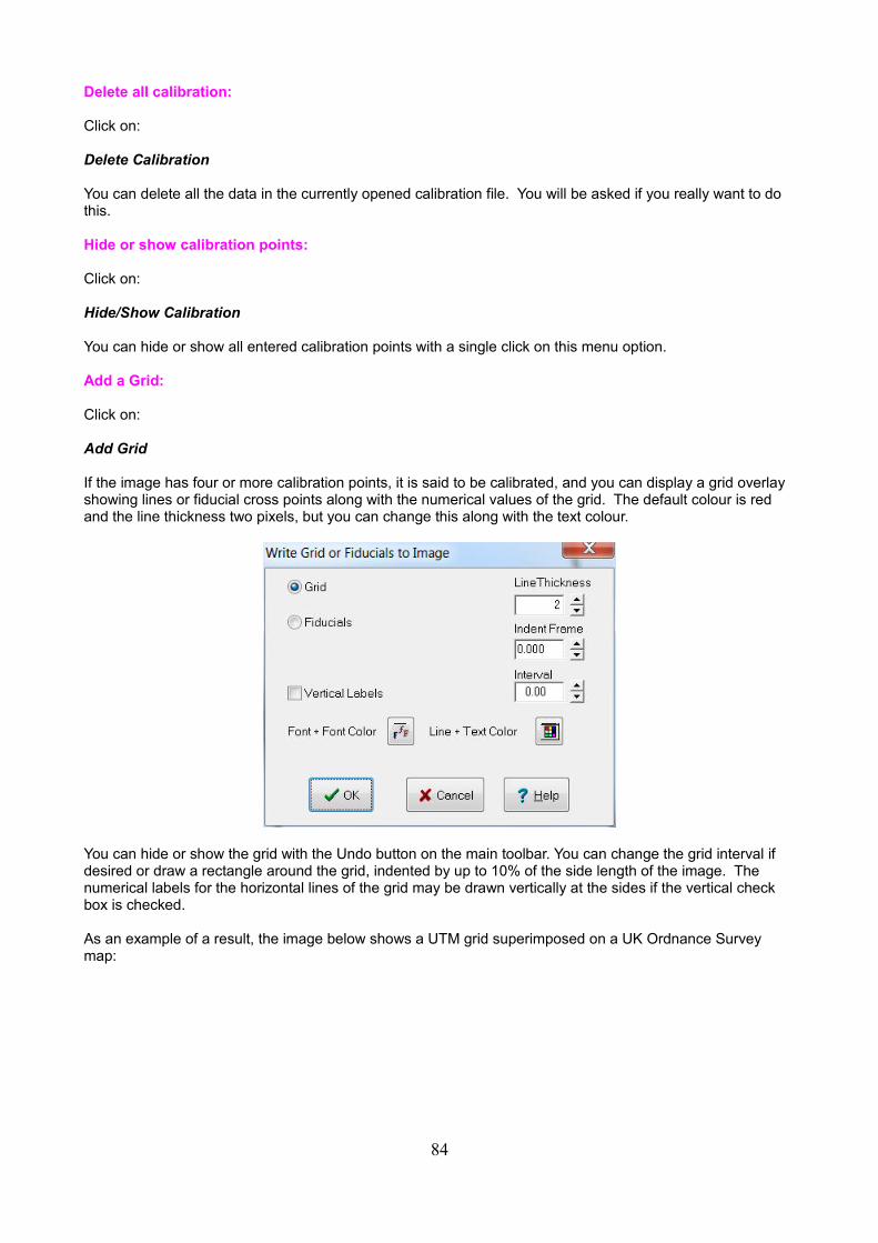
Delete all calibration:

Click on:

Delete Calibration

You can delete all the data in the currently opened calibration file. You will be asked if you really want to do this.

Hide or show calibration points:

Click on:

Hide/Show Calibration

You can hide or show all entered calibration points with a single click on this menu option.

Add a Grid:

Click on:

Add Grid

If the image has four or more calibration points, it is said to be calibrated, and you can display a grid overlay showing lines or fiducial cross points along with the numerical values of the grid. The default colour is red and the line thickness two pixels, but you can change this along with the text colour.

You can hide or show the grid with the Undo button on the main toolbar. You can change the grid interval if desired or draw a rectangle around the grid, indented by up to 10% of the side length of the image. The numerical labels for the horizontal lines of the grid may be drawn vertically at the sides if the vertical check box is checked.

As an example of a result, the image below shows a UTM grid superimposed on a UK Ordnance Survey map:

84

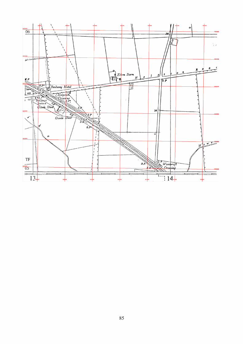
85

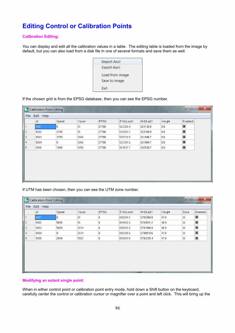
Editing Control or Calibration Points

Calibration Editing: You can display and edit all the calibration values in a table. The editing table is loaded from the image by default, but you can also load from a disk file in one of several formats and save them as well.

If the chosen grid is from the EPSG database, then you can see the EPSG number.

If UTM has been chosen, then you can see the UTM zone number.

Modifying an extant single point:

When in either control point or calibration point entry mode, hold down a Shift button on the keyboard, carefully center the control or calibration cursor or magnifier over a point and left click. This will bring up the

86

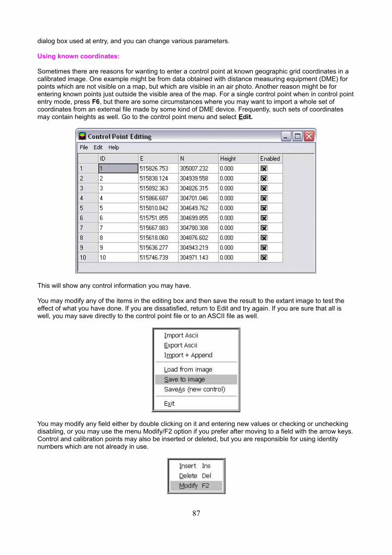
dialog box used at entry, and you can change various parameters.

Using known coordinates:

Sometimes there are reasons for wanting to enter a control point at known geographic grid coordinates in a calibrated image. One example might be from data obtained with distance measuring equipment (DME) for points which are not visible on a map, but which are visible in an air photo. Another reason might be for entering known points just outside the visible area of the map. For a single control point when in control pointentry mode, press F6, but there are some circumstances where you may want to import a whole set of coordinates from an external file made by some kind of DME device. Frequently, such sets of coordinates may contain heights as well. Go to the control point menu and select Edit.

This will show any control information you may have.

You may modify any of the items in the editing box and then save the result to the extant image to test the effect of what you have done. If you are dissatisfied, return to Edit and try again. If you are sure that all is well, you may save directly to the control point file or to an ASCII file as well.

You may modify any field either by double clicking on it and entering new values or checking or unchecking disabling, or you may use the menu Modify/F2 option if you prefer after moving to a field with the arrow keys.Control and calibration points may also be inserted or deleted, but you are responsible for using identity numbers which are not already in use.

87

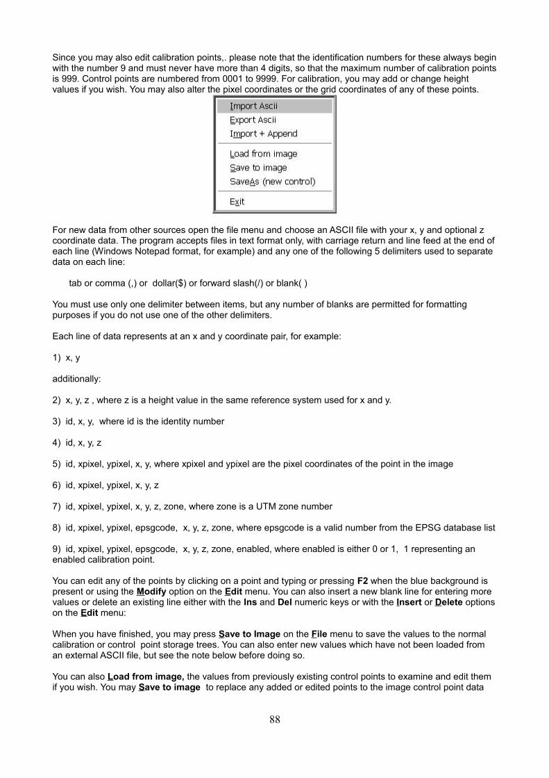
Since you may also edit calibration points,. please note that the identification numbers for these always beginwith the number 9 and must never have more than 4 digits, so that the maximum number of calibration pointsis 999. Control points are numbered from 0001 to 9999. For calibration, you may add or change height values if you wish. You may also alter the pixel coordinates or the grid coordinates of any of these points.

For new data from other sources open the file menu and choose an ASCII file with your x, y and optional z coordinate data. The program accepts files in text format only, with carriage return and line feed at the end ofeach line (Windows Notepad format, for example) and any one of the following 5 delimiters used to separate data on each line:

tab or comma (,) or dollar($) or forward slash(/) or blank( )

You must use only one delimiter between items, but any number of blanks are permitted for formatting purposes if you do not use one of the other delimiters.

Each line of data represents at an x and y coordinate pair, for example:

1) x, y

additionally:

2) x, y, z , where z is a height value in the same reference system used for x and y.

3) id, x, y, where id is the identity number

4) id, x, y, z

5) id, xpixel, ypixel, x, y, where xpixel and ypixel are the pixel coordinates of the point in the image

6) id, xpixel, ypixel, x, y, z

7) id, xpixel, ypixel, x, y, z, zone, where zone is a UTM zone number

8) id, xpixel, ypixel, epsgcode, x, y, z, zone, where epsgcode is a valid number from the EPSG database list

9) id, xpixel, ypixel, epsgcode, x, y, z, zone, enabled, where enabled is either 0 or 1, 1 representing an enabled calibration point.

You can edit any of the points by clicking on a point and typing or pressing F2 when the blue background is present or using the Modify option on the Edit menu. You can also insert a new blank line for entering more values or delete an existing line either with the Ins and Del numeric keys or with the Insert or Delete optionson the Edit menu:

When you have finished, you may press Save to Image on the File menu to save the values to the normal calibration or control point storage trees. You can also enter new values which have not been loaded from an external ASCII file, but see the note below before doing so.

You can also Load from image, the values from previously existing control points to examine and edit them if you wish. You may Save to image to replace any added or edited points to the image control point data

88

structure. Please note that this will not be saved to a .ctl file if you close the image using the emergency exit door tool-bit, or use Alt-F4 or the upper left corner tab. You can save to a new set of control points and to the image simultaneously if you use SaveAs (new control). In that case you will be prompted for a new file name to which the data can be saved in binary control point form. You may also Export ASCII a loaded or imported control point set to a new ASCII file. Finally, you may Import + Append to import multiple sets of ASCII control files and add them to any of the data already in the table.

Note:

The active field in the table has a blue background. When you switch to edit mode either by pressing F2 or choosing Modify from the Edit menu or by starting to type in the field, its background changes to grey The editing only becomes effective when you leave the field either by clicking on another with the mouse, or using any of the keypad movement commands. If you close the table before doing so, the change you have made will not be recorded.

When editing a numeric field:

Double click on the field or press F2 to change the active (blue background) field to edit mode (grey background). Type in new values as required. Move back and forth in the field with the arrow keys on the numeric keypad.

<CtrlY>Erase the field's content.<CtrlZ>Restore the field's original content.<Bksp>Erases one character to left of cursor in value.

Navigation in the Edit dialogue box:

With the numeric keypad:

<Home>Move the active cell to the first column.<Left>Move the active cell left to the previous cell.<Right>Move the active cell right to the next cell.<Down>Move the focus to the next row.<Up>Move the active cell up to the previous row.<End>Move the focus to the last column.<PgDn>Move the active cell to the page following the current page.<PgUp>Move the active cell to the previous page.<CtrIHome>Move the focus to the first cell in the table.<CtrIEnd>Move the active cell to the last cell in the table.<CtrlUp>Move the active cell to the top left cell.<CtrlDown>Move the focus to the cell at the bottom right of the table.<CtrlPgUp>Move the active cell to the top of the page.<CtrlPgDn>Move the active cell to the bottom of the page.<F2>Enter exit table edit mode (or just start typing in the active cell)

With the Mouse:

Drag on the scroll bar to bring a row into the visible area if there are more rows than can fit in the dialogue box. Click on any cell to activate it and make it ready for editing. Click on any other cell to confirm the edit.

Warning:

The program makes no checks on the validity of the data you have either imported or entered by hand. It rejects duplicate id numbers and duplicate coordinate values. If you import with four or more fields present, you must administer your id numbers carefully. Zero is not permitted as an id number. You must enter an id number in every row, or the row will not be exported or loaded.

You are strongly advised not to use this method for entering raw control information.

89

Calibrating GeoPortal Variants

Unfortunately there are no standards for the scripts which run a GeoPortal Web site. Each one is different. Therefore a minimal set of tools has been incorporated into AirPhotoSE which permits extracting basic imageand geographic information from most sites for further processing in AirPhotoSE. These use the Windows Clipboard to exchange data between the site and AirPhotoSE.

All appropriate parameters must be set using the GeoPortal itself. AirPhotoSE can not do this directly, since the scripting code of the site is not standardized and is sometimes encrypted. The available parameters often include a choice of grid system, a scale and the theme to be shown, e.g. an orthophoto, a map, namesand other features. Undesired features which should not be visible in output images must be disabled by using the options offered by the GeoPortal.

The keyboard operations used for interchanging values between data entry fields of a GeoPortal site and thecoordinate fields on the upper toolbar of AirPhotoSE include:

In the GeoPortal user-modifiable data fields:

Shift/Home Highlight the content of a field after entering data.Shift/End Highlight the content of a field if the cursor is at the left edge of the field.Ctrl_C Copy the highlighted content of a field to the Clipboard.Del Delete the content of a highlighted field.Ctrl_V Transfer the content of the Clipboard to a field.

AirPhotoSE monitors the Clipboard continuously for any change made in the GeoPortal followed by Ctrl_C and places a coordinate value saved to the Clipboard with Ctrl_C in the upper toolbar field or fields.

Alt + M to set a screen marker at the cursor's position. If coordinates have been written to orcopied from the Clipboard to the East and North fields of the main capture window, they will be written next to the marker as well as in the GeoPortalFiles.txt protocol

file when the programme closes.

In AirPhotoSE:

Tab Copy a modified value in one of the coordinate fields of AirPhoto SE to the Clipboardfrom which it can be entered into the appropriate GeoPortal field using Ctrl_V in that field.

Alt + S Copy the full GeoPortal screen to an overlying layer belonging to AirPhotoSE and display a selection rectangle which may be dragged to and stretched to include an area of interest and exclude items which should not appear in the result. The coloursof the selected area are inverted for better visibility.

Shift/RightClick Opens a file name dialogue box to permit entering a name for a file to contain the first area captured.

RightClick Capture additional areas after moving the underlying GeoPortal image and pressing Alt-S again or clicking on the Save and Capture menu item.

90

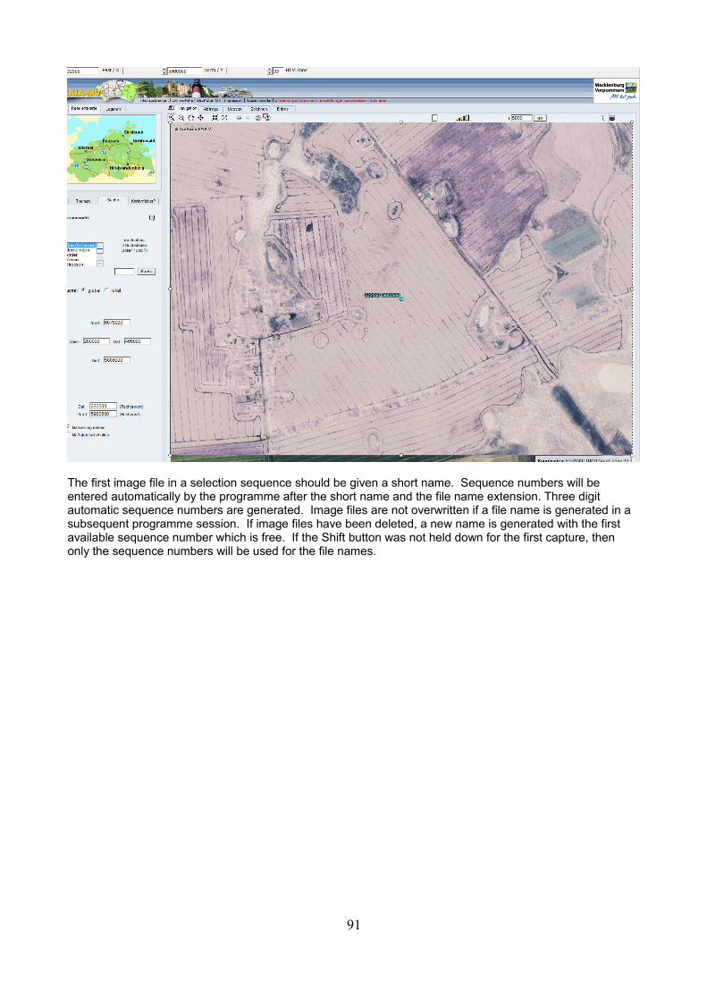
The first image file in a selection sequence should be given a short name. Sequence numbers will be entered automatically by the programme after the short name and the file name extension. Three digit automatic sequence numbers are generated. Image files are not overwritten if a file name is generated in a subsequent programme session. If image files have been deleted, a new name is generated with the first available sequence number which is free. If the Shift button was not held down for the first capture, then only the sequence numbers will be used for the file names.

91

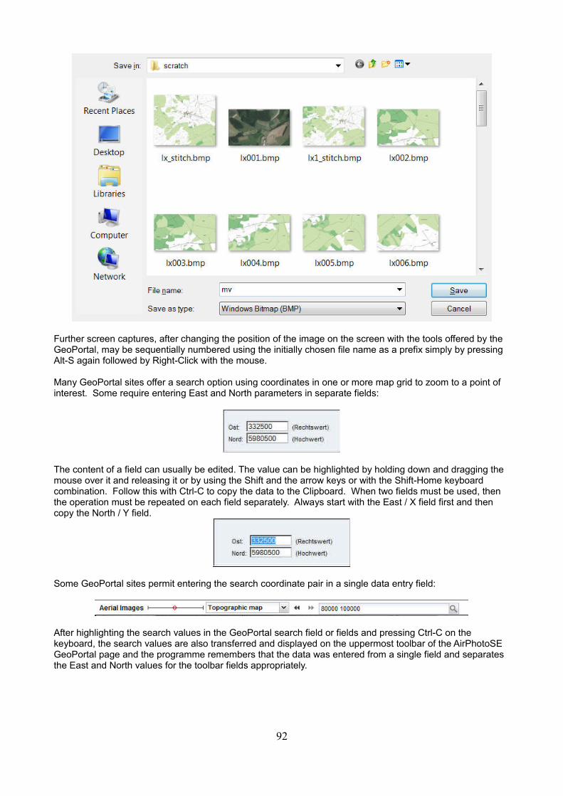
Further screen captures, after changing the position of the image on the screen with the tools offered by the GeoPortal, may be sequentially numbered using the initially chosen file name as a prefix simply by pressing Alt-S again followed by Right-Click with the mouse.

Many GeoPortal sites offer a search option using coordinates in one or more map grid to zoom to a point of interest. Some require entering East and North parameters in separate fields:

The content of a field can usually be edited. The value can be highlighted by holding down and dragging the mouse over it and releasing it or by using the Shift and the arrow keys or with the Shift-Home keyboard combination. Follow this with Ctrl-C to copy the data to the Clipboard. When two fields must be used, then the operation must be repeated on each field separately. Always start with the East / X field first and then copy the North / Y field.

Some GeoPortal sites permit entering the search coordinate pair in a single data entry field:

After highlighting the search values in the GeoPortal search field or fields and pressing Ctrl-C on the keyboard, the search values are also transferred and displayed on the uppermost toolbar of the AirPhotoSE GeoPortal page and the programme remembers that the data was entered from a single field and separates the East and North values for the toolbar fields appropriately.

92

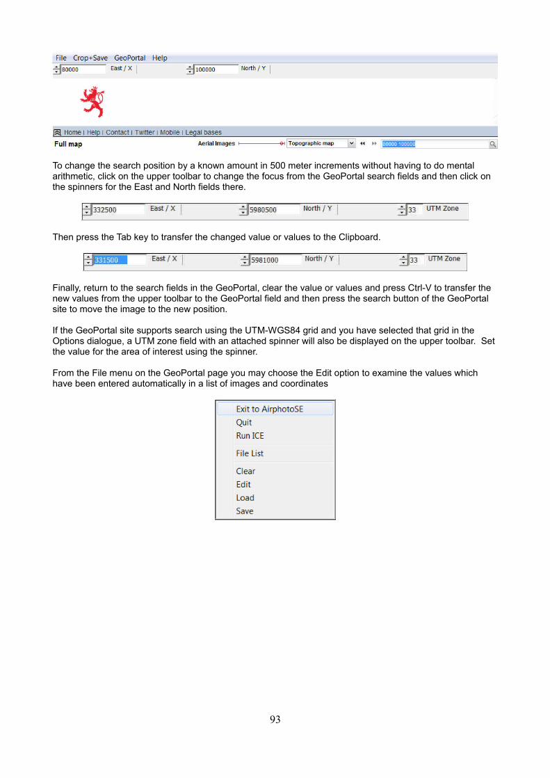
To change the search position by a known amount in 500 meter increments without having to do mental arithmetic, click on the upper toolbar to change the focus from the GeoPortal search fields and then click on the spinners for the East and North fields there.

Then press the Tab key to transfer the changed value or values to the Clipboard.

Finally, return to the search fields in the GeoPortal, clear the value or values and press Ctrl-V to transfer the new values from the upper toolbar to the GeoPortal field and then press the search button of the GeoPortal site to move the image to the new position.

If the GeoPortal site supports search using the UTM-WGS84 grid and you have selected that grid in the Options dialogue, a UTM zone field with an attached spinner will also be displayed on the upper toolbar. Set the value for the area of interest using the spinner.

From the File menu on the GeoPortal page you may choose the Edit option to examine the values which have been entered automatically in a list of images and coordinates

93

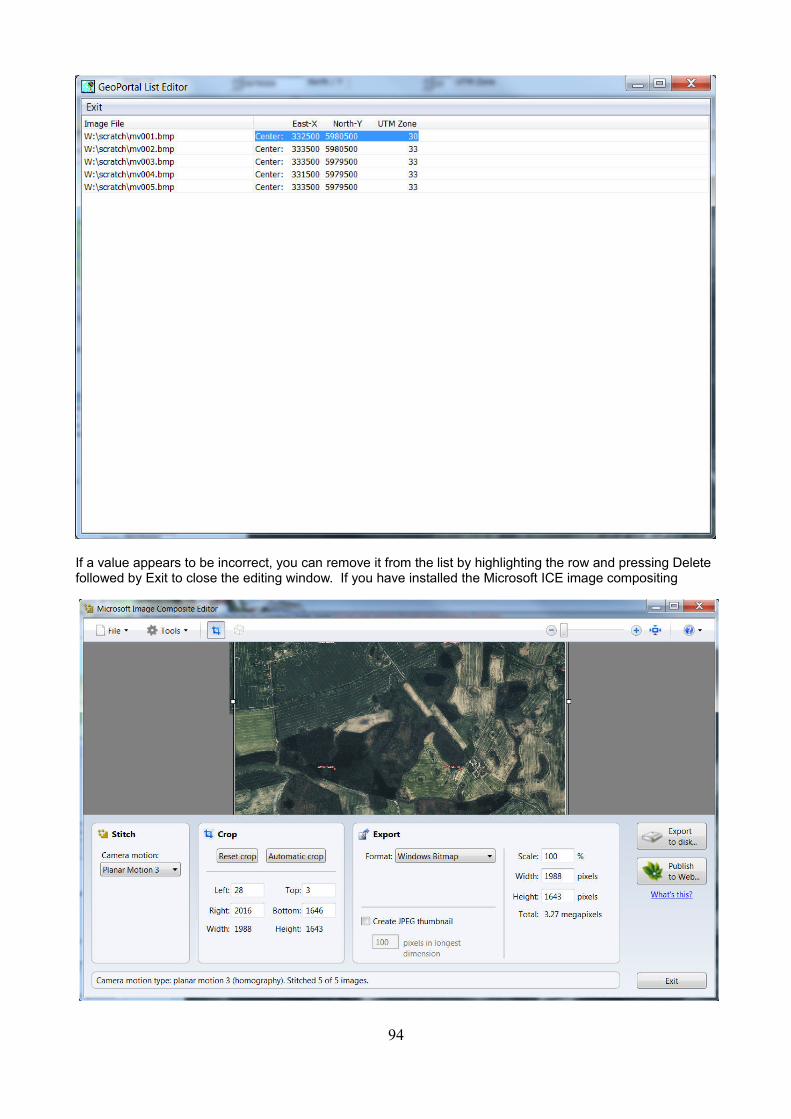
If a value appears to be incorrect, you can remove it from the list by highlighting the row and pressing Delete followed by Exit to close the editing window. If you have installed the Microsoft ICE image compositing

94

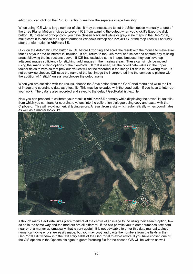
editor, you can click on the Run ICE entry to see how the separate image tiles align

When using ICE with a large number of tiles, it may be necessary to set the Stitch option manually to one of the three Planar Motion choices to prevent ICE from warping the output when you click it's Export to disk button. If, instead of orthophotos, you have chosen black and white or grey-scale maps in the GeoPortal, make certain to choose the Export format as Windows Bitmap and not JPEG, or the map lines will be fuzzy after transformation in AirPhotoSE.

Click on the Automatic Crop button in ICE before Exporting and scroll the result with the mouse to make surethat all of your area of interest is included. If not, return to the GeoPortal and select and capture any missingareas following the instructions above. If ICE has excluded some images because they don't overlap adjacent images sufficiently for stitching, add images in the missing areas. These can simply be moved using the image shifting options of the GeoPortal. If that is used, set the coordinate values in the upper toolbar fields to zero so that previous values will not be recorded in the image list data in the wrong rows. If not otherwise chosen, ICE uses the name of the last image tile incorporated into the composite picture with the addition of "_stitch" unless you choose the output name.

When you are satisfied with the results, choose the Save option from the GeoPortal menu and write the list of image and coordinate data as a text file. This may be reloaded with the Load option if you have to interruptyour work. The data is also recorded and saved to the default GeoPortal list text file.

Now you can proceed to calibrate your result in AirPhotoSE normally while displaying the saved list text file from which you can transfer coordinate values into the calibration dialogue using copy and paste with the Clipboard. This will avoid numerical typing errors. A result from a site which automatically writes coordinates as well as a marker looks like:

Although many GeoPortal sites place markers at the centre of an image found using their search option, few do so in the same way and the markers are all different. If the site permits you to enter numerical text data near or at a marker automatically, that is very useful. It is not advisable to enter this data manually, since numerical typing errors are easily made, but you may copy and paste the numbers from the fields in the GeoPortal Edit window into the text entry fields of the GeoPortal to avoid errors. If you have chosen one of the GIS options in the Options dialogue, a georeferencing file for the chosen GIS will be written as well

95

Special Capture Window

The special capture window is enabled when the short name given for a GeoPortal is followed by [sc] before the URL which must always begin with http://

Example:

BadenWurttemberg [sc] http://www.geoportal.lv-bw.de/mapbender/

The four text characters may be inserted in any Geoportal link with a text editor like Windows Notepad on thefile

geoportalurls.txt

which can be found on the installation directory.

The special capture window is needed when the GeoPortal shows a separate preliminary window before a map or an orthophoto can be displayed. Commonly, this is to require the user to accept the terms and conditions of the GeoPortal's owners, but it may also be useful if a full screen view is shown using a separateprogramme like Adobe Shockwave or Flash.

Before opening the second window of the GeoPortal, the special capture window should be opened either bypressing Ctrl-F12 or clicking on the Special Capture menu entry on the initial GeoPortal display window.

The following keyboard short-cuts are used in the special capture window so that the position of the mouse cursor need not be changed when capturing, thus permitting visible coordinates or other values which are changed by the mouse cursor's position to be captured correctly.

Keyboard Short-cuts:

Ctrl+F12 to initialize the special capture window. This need only be done once.

Ctrl+F10 Capture an Area (or Ctrl+F8 if Ctrl+F10 in use)

Ctrl+F11 Capture the Full Screen (or Ctrl+F9 if Ctrl+F11 in use)

Ctrl + M to set a screen marker at the cursor's position. If coordinates have been written to or copied from the Clipboard to the East and North fields of the main capture window, they will be written next to the marker as well as in the GeoPortalFiles.txt protocol file when the programme closes.

If a background map shows a grid, this makes placement and transfer of values for a marker much easier. If coordinates are shown by the site as the mouse is moved, pressing Alt+S to capture the image leaves the coordinates unchanged, and these can be typed into the East and North fields, or copied to the Clipboard if they are shown in the search fields of the site.

96

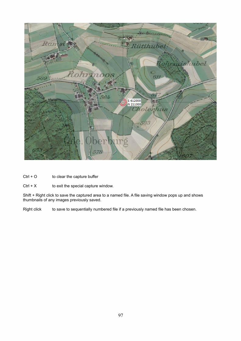
Ctrl + O to clear the capture buffer

Ctrl + X to exit the special capture window.

Shift + Right click to save the captured area to a named file. A file saving window pops up and shows thumbnails of any images previously saved.

Right click to save to sequentially numbered file if a previously named file has been chosen.

97

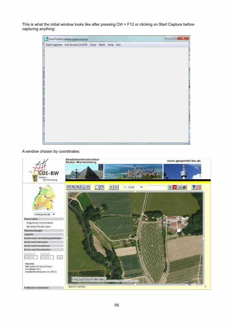
This is what the initial window looks like after pressing Ctrl + F12 or clicking on Start Capture before capturing anything:

A window chosen by coordinates:

98

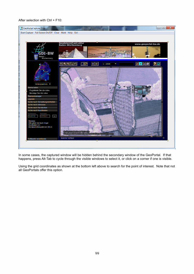
After selection with Ctrl + F10:

In some cases, the captured window will be hidden behind the secondary window of the GeoPortal. If that happens, press Alt-Tab to cycle through the visible windows to select it, or click on a corner if one is visible.

Using the grid coordinates as shown at the bottom left above to search for the point of interest. Note that notall GeoPortals offer this option.

99

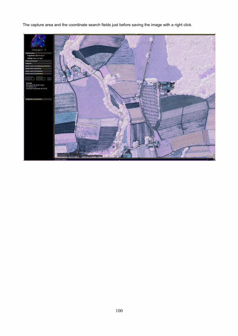
The capture area and the coordinate search fields just before saving the image with a right click.

100

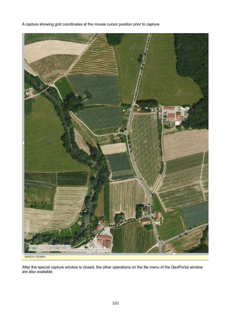
A capture showing grid coordinates at the mouse cursor position prior to capture

After the special capture window is closed, the other operations on the file menu of the GeoPortal window are also available.

101

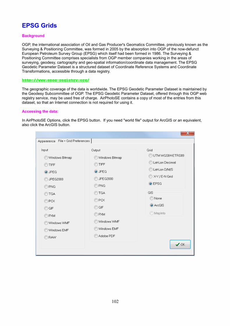
EPSG Grids

Background

OGP, the international association of Oil and Gas Producer's Geomatics Committee, previously known as theSurveying & Positioning Committee, was formed in 2005 by the absorption into OGP of the now-defunct European Petroleum Survey Group (EPSG) which itself had been formed in 1986. The Surveying & Positioning Committee comprises specialists from OGP member companies working in the areas of surveying, geodesy, cartography and geo-spatial information/coordinate data management. The EPSG Geodetic Parameter Dataset is a structured dataset of Coordinate Reference Systems and Coordinate Transformations, accessible through a data registry.

http://www.epsg-registry.org/

The geographic coverage of the data is worldwide. The EPSG Geodetic Parameter Dataset is maintained by the Geodesy Subcommittee of OGP. The EPSG Geodetic Parameter Dataset, offered through this OGP web registry service, may be used free of charge. AirPhotoSE contains a copy of most of the entries from this dataset, so that an Internet connection is not required for using it.

Accessing the data:

In AirPhotoSE Options, click the EPSG button. If you need "world file" output for ArcGIS or an equivalent, also click the ArcGIS button.

102

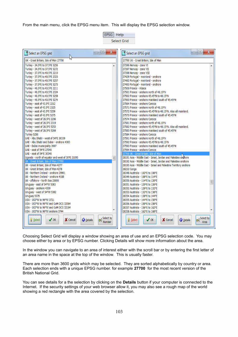
From the main menu, click the EPSG menu item. This will display the EPSG selection window.

Choosing Select Grid will display a window showing an area of use and an EPSG selection code. You may choose either by area or by EPSG number. Clicking Details will show more information about the area.

In the window you can navigate to an area of interest either with the scroll bar or by entering the first letter of an area name in the space at the top of the window. This is usually faster.

There are more than 3600 grids which may be selected. They are sorted alphabetically by country or area. Each selection ends with a unique EPSG number. for example 27700 for the most recent version of the British National Grid.

You can see details for a the selection by clicking on the Details button if your computer is connected to the Internet. If the security settings of your web browser allow it, you may also see a rough map of the world showing a red rectangle with the area covered by the selection.

103

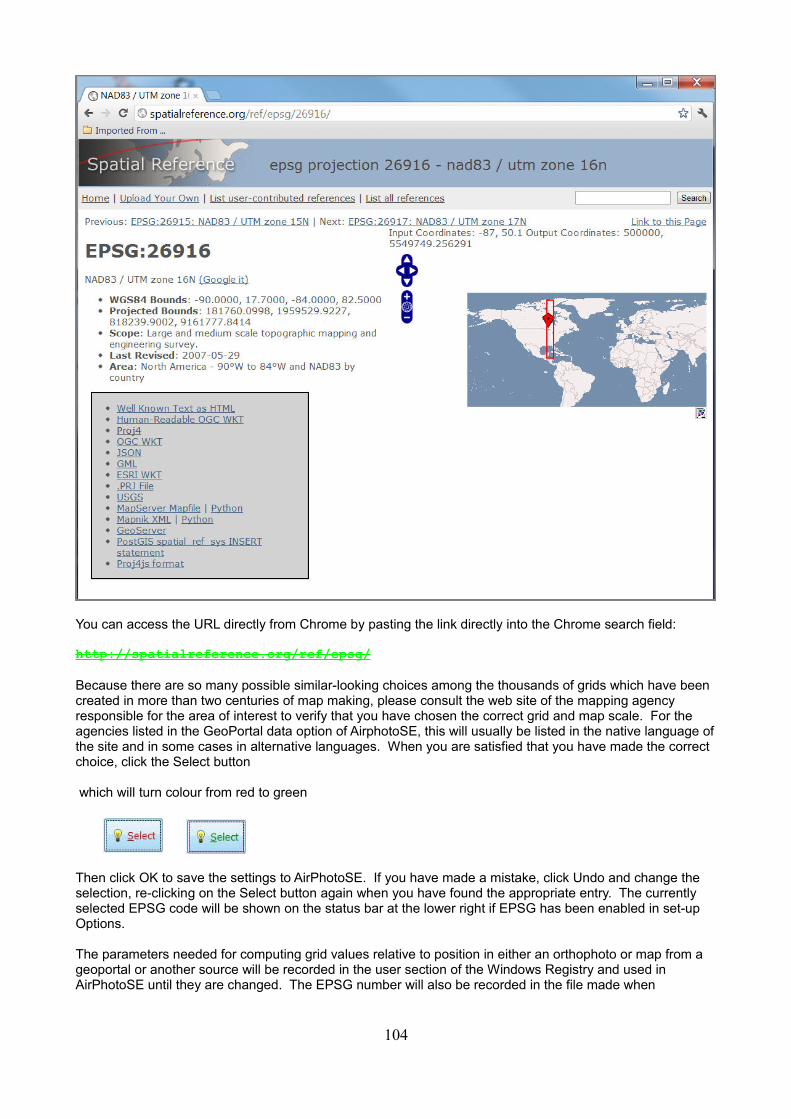
You can access the URL directly from Chrome by pasting the link directly into the Chrome search field:

http://spatialreference.org/ref/epsg/

Because there are so many possible similar-looking choices among the thousands of grids which have been created in more than two centuries of map making, please consult the web site of the mapping agency responsible for the area of interest to verify that you have chosen the correct grid and map scale. For the agencies listed in the GeoPortal data option of AirphotoSE, this will usually be listed in the native language ofthe site and in some cases in alternative languages. When you are satisfied that you have made the correct choice, click the Select button

which will turn colour from red to green

Then click OK to save the settings to AirPhotoSE. If you have made a mistake, click Undo and change the selection, re-clicking on the Select button again when you have found the appropriate entry. The currently selected EPSG code will be shown on the status bar at the lower right if EPSG has been enabled in set-up Options.

The parameters needed for computing grid values relative to position in either an orthophoto or map from a geoportal or another source will be recorded in the user section of the Windows Registry and used in AirPhotoSE until they are changed. The EPSG number will also be recorded in the file made when

104

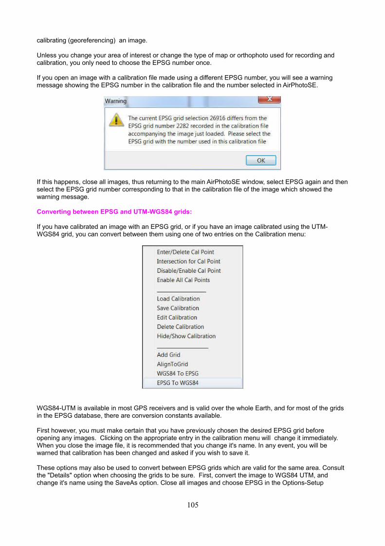
calibrating (georeferencing) an image.

Unless you change your area of interest or change the type of map or orthophoto used for recording and calibration, you only need to choose the EPSG number once.

If you open an image with a calibration file made using a different EPSG number, you will see a warning message showing the EPSG number in the calibration file and the number selected in AirPhotoSE.

If this happens, close all images, thus returning to the main AirPhotoSE window, select EPSG again and thenselect the EPSG grid number corresponding to that in the calibration file of the image which showed the warning message.

Converting between EPSG and UTM-WGS84 grids:

If you have calibrated an image with an EPSG grid, or if you have an image calibrated using the UTM-WGS84 grid, you can convert between them using one of two entries on the Calibration menu:

WGS84-UTM is available in most GPS receivers and is valid over the whole Earth, and for most of the grids in the EPSG database, there are conversion constants available.

First however, you must make certain that you have previously chosen the desired EPSG grid before opening any images. Clicking on the appropriate entry in the calibration menu will change it immediately. When you close the image file, it is recommended that you change it's name. In any event, you will be warned that calibration has been changed and asked if you wish to save it.

These options may also be used to convert between EPSG grids which are valid for the same area. Consult the "Details" option when choosing the grids to be sure. First, convert the image to WGS84 UTM, and change it's name using the SaveAs option. Close all images and choose EPSG in the Options-Setup

105

dialogue, and then choose the desired new grid. Open the image saved with the WGS84-UTM grid, and click on the WGS84toEPSG menu entry, and save it again.

Depending on the accuracy of the constants for transformation between EPSG and WGS84 grids supplied inthe EPSG database, there may be small differences in observed coordinates. If an image has already been converted, then you will see an information dialogue informing you of this, and nothing will be changed. If you are saving from WGS84-UTM to EPSG and the calibration points of your image lie outside the valid areafor the EPSG grid chosen, no changes will be made either.

106

Google Earth Pro Installation

In AirPhotoSE, the professional version of Google Earth is now supported as well as the standard version.. Ifinstalled, it will be used in preference to the standard version of Google Earth.

It can be downloaded without charge from:

https://support.google.com/earth/answer/176160?hl=en

After downloading and installation, you will be asked for your e-mail address and the password GEPREE

Check the auto login box on the registration form so that you will only need to do this once.

The Pro version offers options for saving images with high resolution and other useful GIS additions to the standard version of Google Earth.

See:

Google Earth Pro Users Guide

and

Importing GIS Datal

107

The Google Earth Pro application form:

Noie:

in AirPhotoSE prior to version 2.62, Google Earth used the Google Earth Web Browser Plugin. The plugin was installed automatically when the standard Google Earth client was installed. As of December 15, 2015, Google removed support for the plugin for security reasons, but it may continue to operate for an unspecified time. The Google Earth Plugin does not work on machines using Windows 10.

108

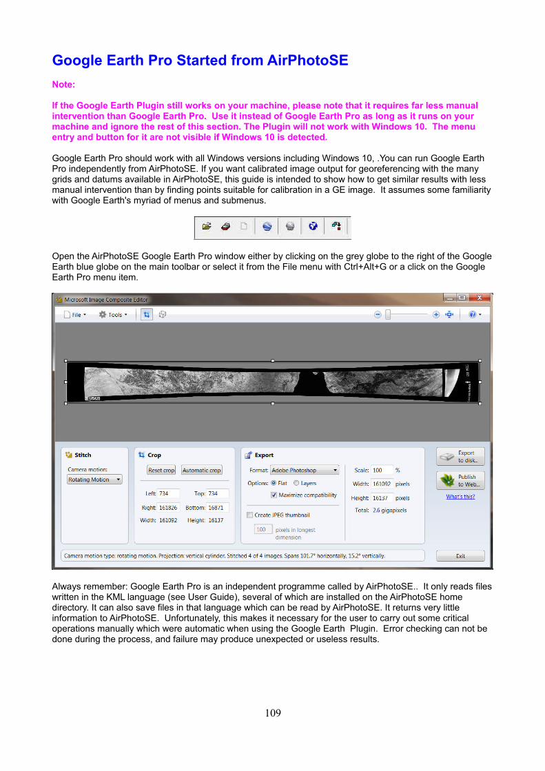
Google Earth Pro Started from AirPhotoSE

Note:

If the Google Earth Plugin still works on your machine, please note that it requires far less manual intervention than Google Earth Pro. Use it instead of Google Earth Pro as long as it runs on your machine and ignore the rest of this section. The Plugin will not work with Windows 10. The menu entry and button for it are not visible if Windows 10 is detected.

Google Earth Pro should work with all Windows versions including Windows 10, .You can run Google Earth Pro independently from AirPhotoSE. If you want calibrated image output for georeferencing with the many grids and datums available in AirPhotoSE, this guide is intended to show how to get similar results with less manual intervention than by finding points suitable for calibration in a GE image. It assumes some familiaritywith Google Earth's myriad of menus and submenus.

Open the AirPhotoSE Google Earth Pro window either by clicking on the grey globe to the right of the GoogleEarth blue globe on the main toolbar or select it from the File menu with Ctrl+Alt+G or a click on the Google Earth Pro menu item.

Always remember: Google Earth Pro is an independent programme called by AirPhotoSE.. It only reads fileswritten in the KML language (see User Guide), several of which are installed on the AirPhotoSE home directory. It can also save files in that language which can be read by AirPhotoSE. It returns very little information to AirPhotoSE. Unfortunately, this makes it necessary for the user to carry out some critical operations manually which were automatic when using the Google Earth Plugin. Error checking can not be done during the process, and failure may produce unexpected or useless results.

109

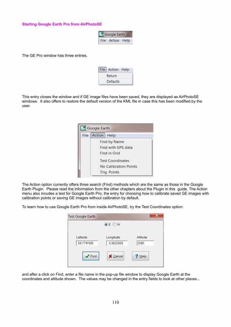
Starting Google Earth Pro from AirPhotoSE

The GE Pro window has three entries.

This entry closes the window and if GE image files have been saved, they are displayed as AirPhotoSE windows. It also offers to restore the default version of the KML file in case this has been modified.by the user.

The Action option currently offers three search (Find) methods which are the same as those in the Google Earth Plugin. Please read the information from the other chapters about the Plugin in this guide. The Action menu also incudes a test for Google Earth Pro, the entry for choosing how to calibrate saved GE images withcalibration points or saving GE images without calibration by default.

To learn how to use Google Earth Pro from inside AirPhotoSE, try the Test Coordinates option:

and after a click on Find, enter a file name in the pop-up file window to display Google Earth at the coordinates and altitude shown. The values may be changed in the entry fields to look at other places...

110

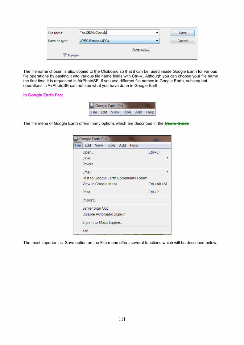
The file name chosen is also copied to the Clipboard so that it can be used inside Google Earth for various file operations by pasting it into various file name fields with Ctrl-V.. Although you can choose your file name the first time it is requested in AirPhotoSE, if you use different file names in Google Earth, subsequent operations in AirPhotoSE can not see what you have done in Google Earth.

In Google Earth Pro:

The file menu of Google Earth offers many options which are described in the Users Guide

The most important is Save option on the File menu offers several functions which will be described below.

111

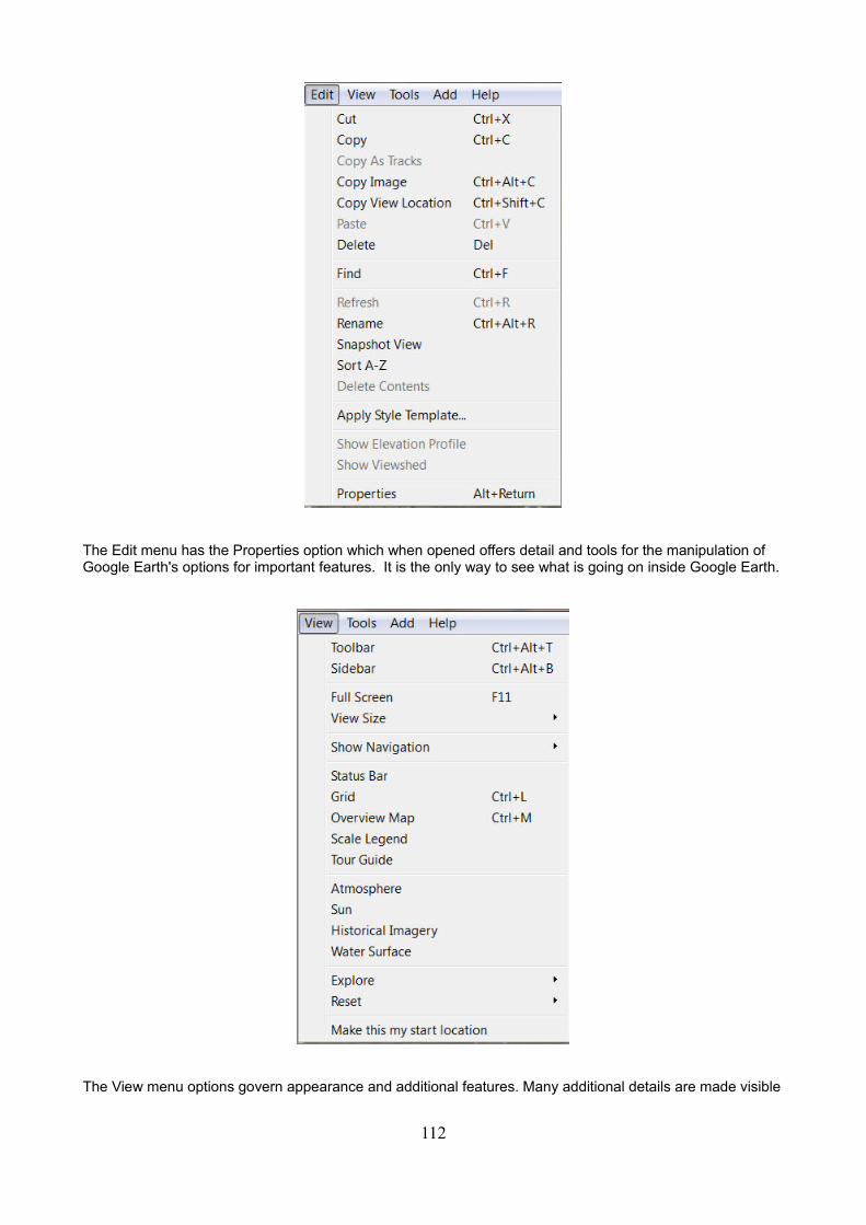
The Edit menu has the Properties option which when opened offers detail and tools for the manipulation of Google Earth's options for important features. It is the only way to see what is going on inside Google Earth.

The View menu options govern appearance and additional features. Many additional details are made visible

112

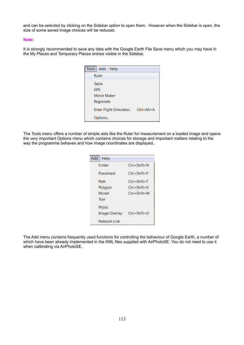
and can be selected by clicking on the Sidebar option to open them. However when the Sidebar is open, thesize of some saved image choices will be reduced.

Note:

It is strongly recommended to save any data with the Google Earth File Save menu which you may have in the My Places and Temporary Places entries visible in the Sidebar,

The Tools menu offers a number of simple aids like the Ruler for measurement on a loaded image and opensthe very important Options menu which contains choices for storage and important matters relating to the way the programme behaves and how image coordinates are displayed..

The Add menu contains frequently used functions for controlling the behaviour of Google Earth, a number of which have been already implemented in the KML files supplied with AirPhotoSE. You do not need to use it when calibrating via AirPhotoSE.

113

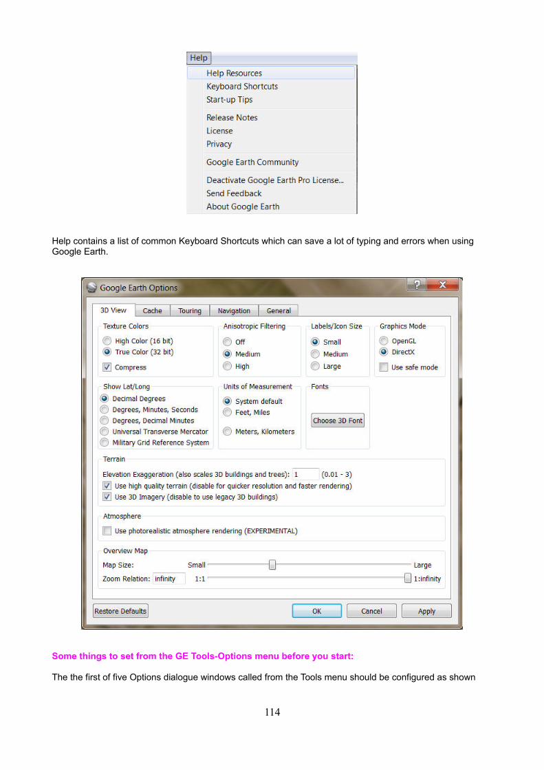
Help contains a list of common Keyboard Shortcuts which can save a lot of typing and errors when using Google Earth.

Some things to set from the GE Tools-Options menu before you start:

The the first of five Options dialogue windows called from the Tools menu should be configured as shown

114

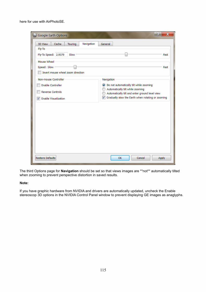
here for use with AirPhotoSE.

The third Options page for Navigation should be set so that views images are **not** automatically tilted when zooming to prevent perspective distortion in saved results.

Note:

If you have graphic hardware from NVIDIA and drivers are automatically updated, uncheck the Enable stereoscop 3D options in the NVIDIA Control Panel window to prevent displaying GE images as anaglyphs.

115

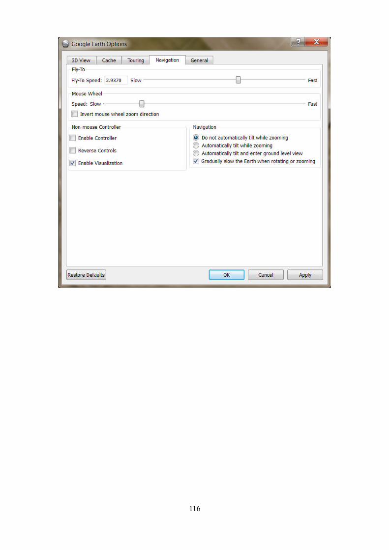
116

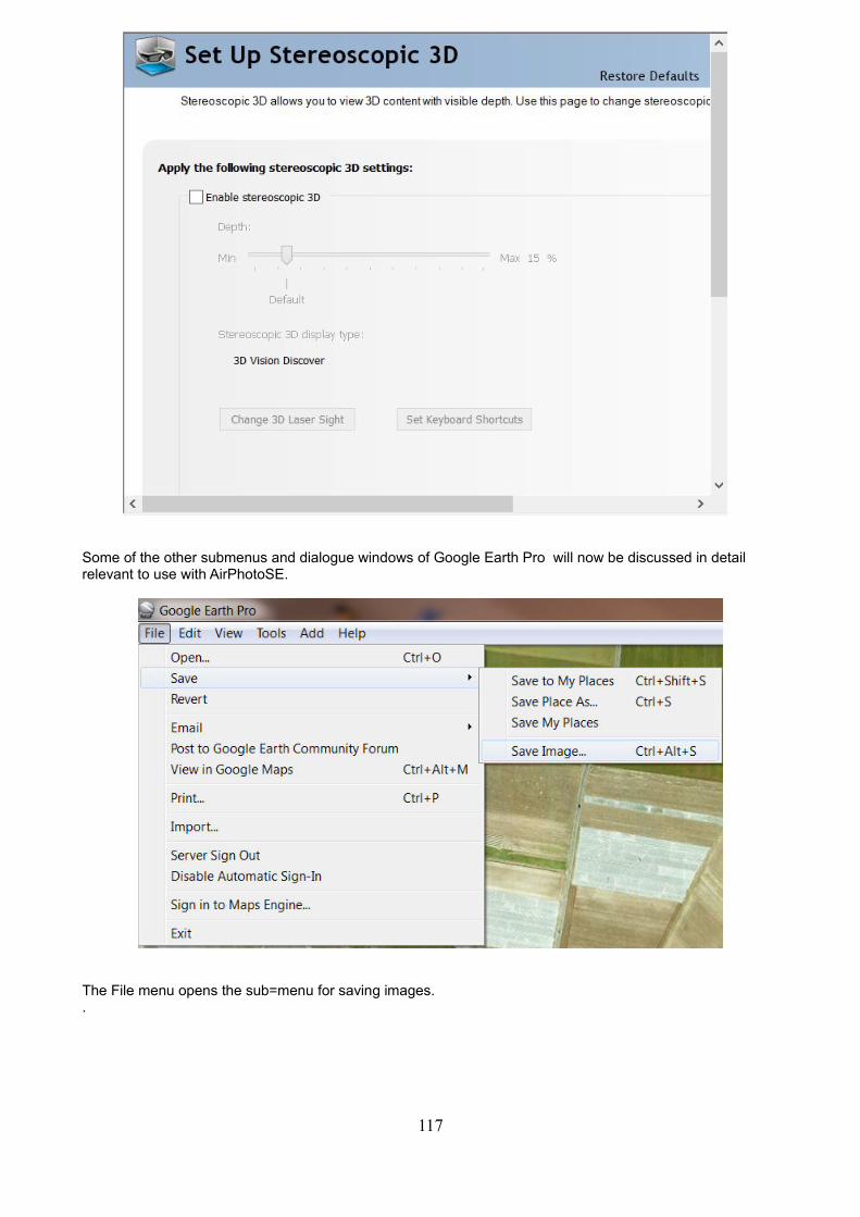
Some of the other submenus and dialogue windows of Google Earth Pro will now be discussed in detail relevant to use with AirPhotoSE.

The File menu opens the sub=menu for saving images..

117

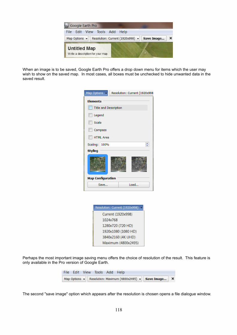
When an image is to be saved, Google Earth Pro offers a drop down menu for items which the user may wish to show on the saved map. In most cases, all boxes must be unchecked to hide unwanted data in the saved result.

Perhaps the most important image saving menu offers the choice of resolution of the result. This feature is only available in the Pro version of Google Earth.

The second "save image" option which appears after the resolution is chosen opens a file dialogue window.

118

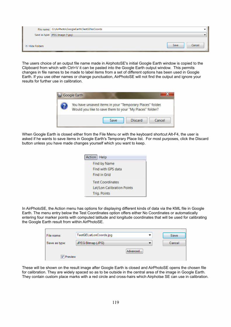
The users choice of an output file name made in AirphotoSE's initial Google Earth window is copied to the Clipboard from which with Ctrl=V it can be pasted into the Google Earth output window. This permits changes in file names to be made to label items from a set of different options has been used in Google Earth. If you use other names or change punctuation, AirPhotoSE will not find the output and ignore your results for further use in calibration.

When Google Earth is closed either from the File Menu or with the keyboard shortcut Alt-F4, the user is asked if he wants to save items in Google Earth's Temporary Place list. For most purposes, click the Discardbutton unless you have made changes yourself which you want to keep.

In AirPhotoSE, the Action menu has options for displaying different kinds of data via the KML file in Google Earth. The menu entry below the Test Coordinates option offers either No Coordinates or automatically entering four marker points with computed latitude and longitude coordinates that will be used for calibrating the Google Earth result from within AirPhotoSE.

These will be shown on the result image after Google Earth is closed and AirPhotoSE opens the chosen file for calibration. They are widely spaced so as to be outside in the central area of the image in Google Earth. They contain custom place marks with a red circle and cross-hairs which Airphotse SE can use in calibration.

119

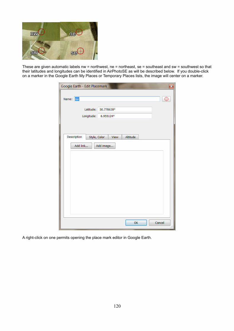
These are given automatic labels nw = northwest, ne = northeast, se = southeast and sw = southwest so thattheir latitudes and longitudes can be identified in AirPhotoSE as will be described below. If you double-click on a marker in the Google Earth My Places or Temporary Places lists, the image will center on a marker.

A right-click on one permits opening the place mark editor in Google Earth.

120

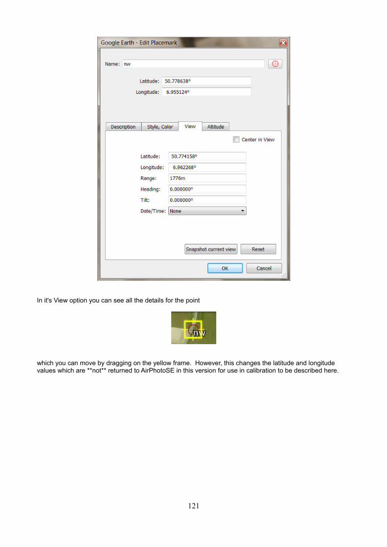
In it's View option you can see all the details for the point

which you can move by dragging on the yellow frame. However, this changes the latitude and longitude values which are **not** returned to AirPhotoSE in this version for use in calibration to be described here.

121

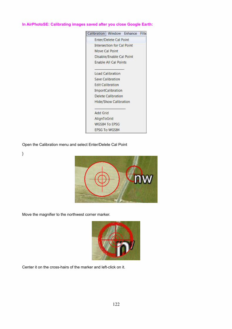
In AirPhotoSE: Calibrating images saved after you close Google Earth:

Open the Calibration menu and select Enter/Delete Cal Point

}

Move the magnifier to the northwest corner marker.

Center it on the cross-hairs of the marker and left-click on it.

122

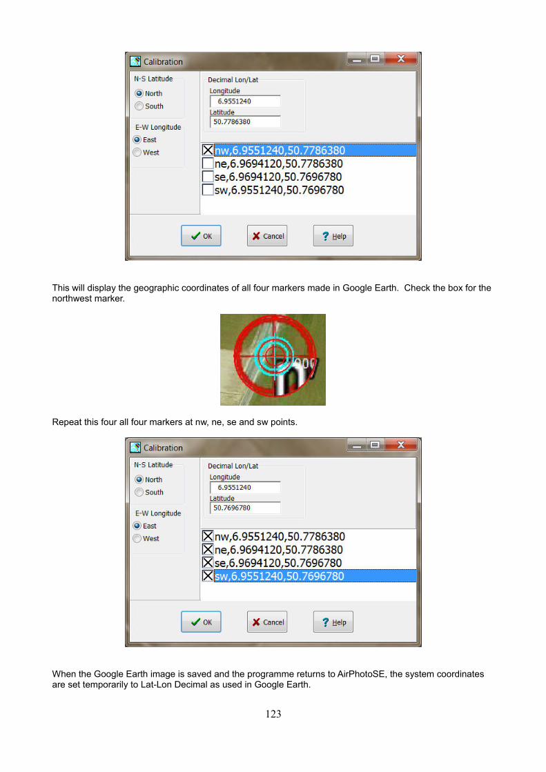
This will display the geographic coordinates of all four markers made in Google Earth. Check the box for the northwest marker.

Repeat this four all four markers at nw, ne, se and sw points.

When the Google Earth image is saved and the programme returns to AirPhotoSE, the system coordinates are set temporarily to Lat-Lon Decimal as used in Google Earth.

123

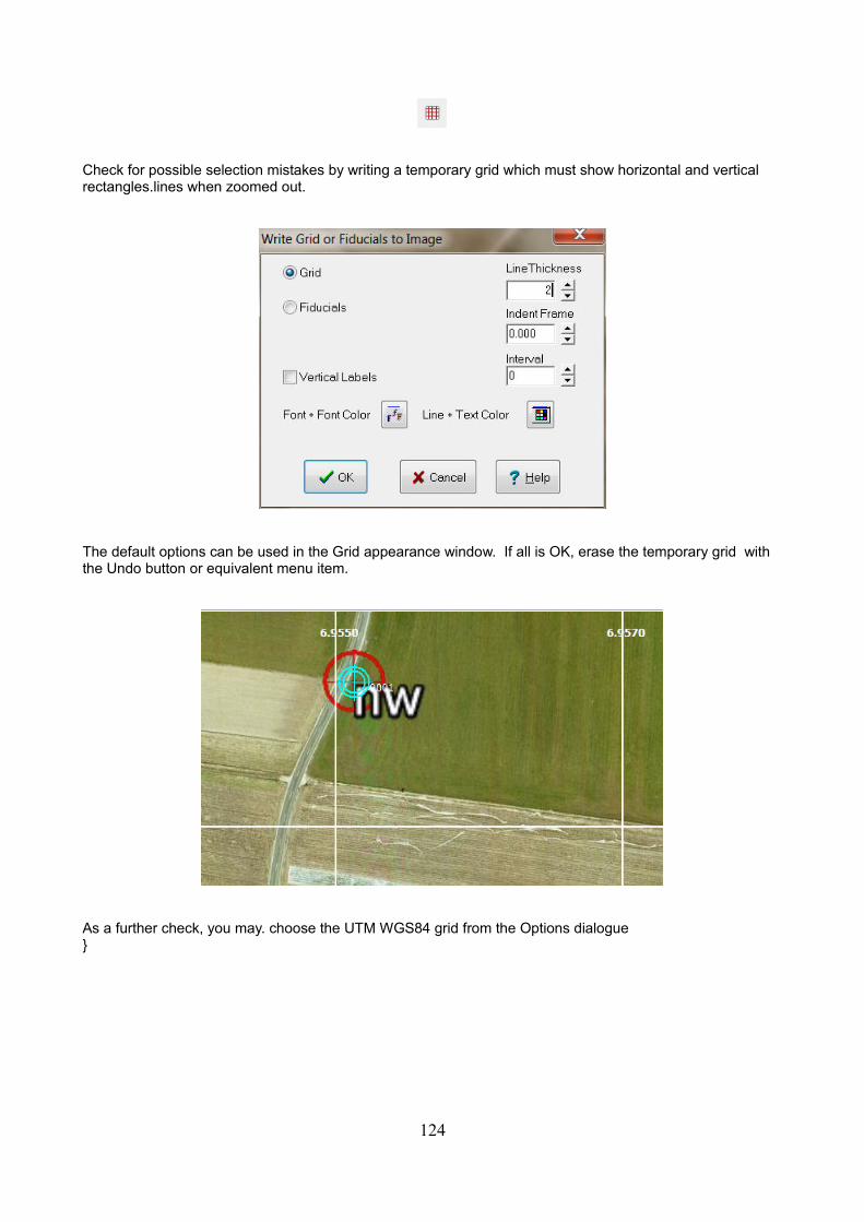
Check for possible selection mistakes by writing a temporary grid which must show horizontal and vertical rectangles.lines when zoomed out.

The default options can be used in the Grid appearance window. If all is OK, erase the temporary grid with the Undo button or equivalent menu item.

As a further check, you may. choose the UTM WGS84 grid from the Options dialogue}

124

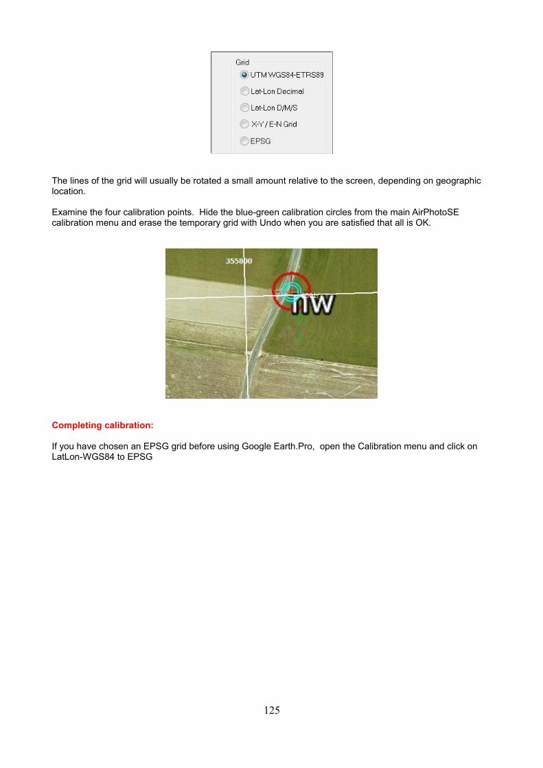
The lines of the grid will usually be rotated a small amount relative to the screen, depending on geographic location.

Examine the four calibration points. Hide the blue-green calibration circles from the main AirPhotoSE calibration menu and erase the temporary grid with Undo when you are satisfied that all is OK.

Completing calibration:

If you have chosen an EPSG grid before using Google Earth.Pro, open the Calibration menu and click on LatLon-WGS84 to EPSG

125

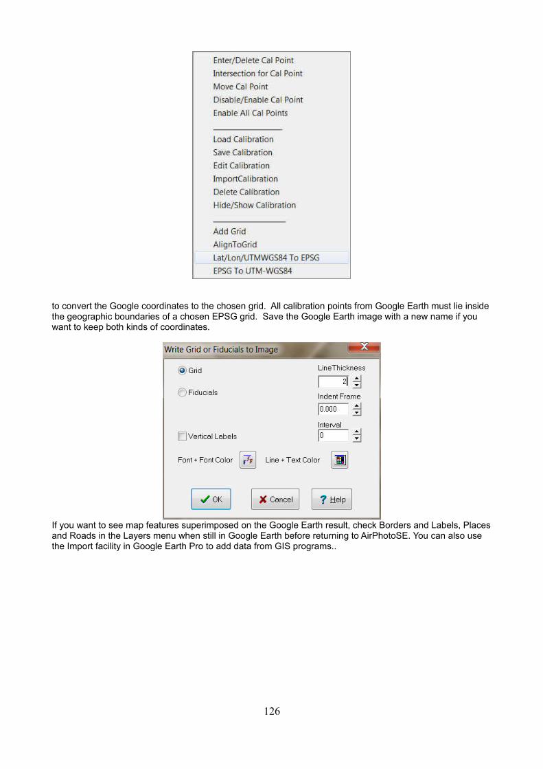
to convert the Google coordinates to the chosen grid. All calibration points from Google Earth must lie insidethe geographic boundaries of a chosen EPSG grid. Save the Google Earth image with a new name if you want to keep both kinds of coordinates.

If you want to see map features superimposed on the Google Earth result, check Borders and Labels, Placesand Roads in the Layers menu when still in Google Earth before returning to AirPhotoSE. You can also use the Import facility in Google Earth Pro to add data from GIS programs..

126

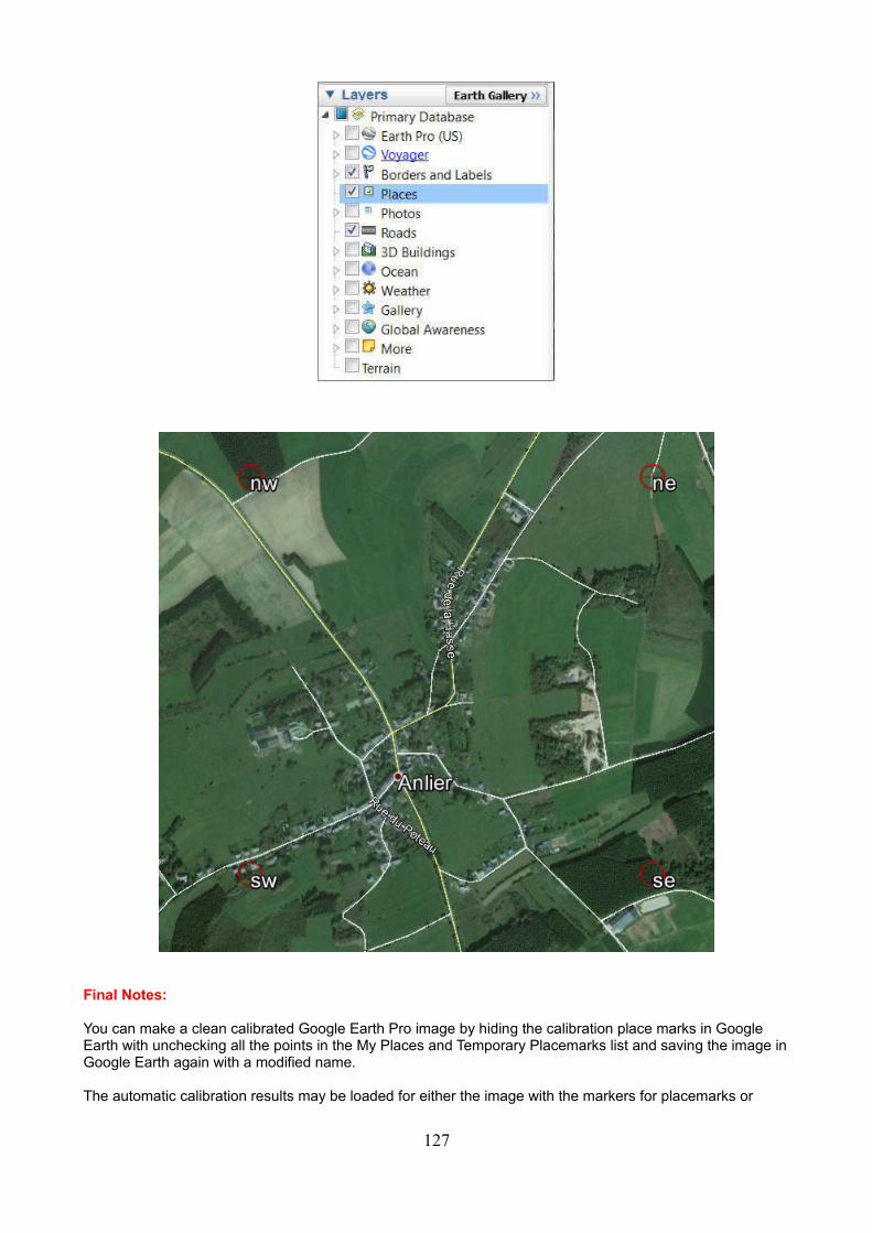
Final Notes:

You can make a clean calibrated Google Earth Pro image by hiding the calibration place marks in Google Earth with unchecking all the points in the My Places and Temporary Placemarks list and saving the image inGoogle Earth again with a modified name.

The automatic calibration results may be loaded for either the image with the markers for placemarks or

127

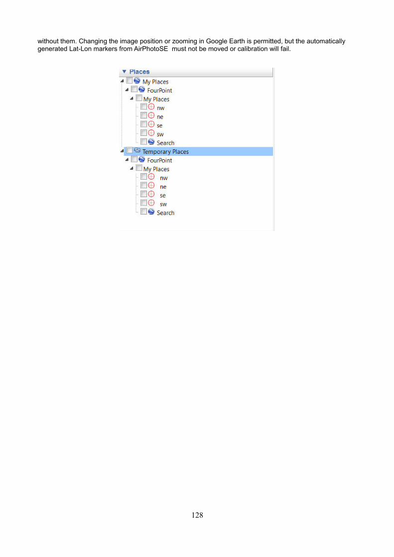
without them. Changing the image position or zooming in Google Earth is permitted, but the automatically generated Lat-Lon markers from AirPhotoSE must not be moved or calibration will fail.

128

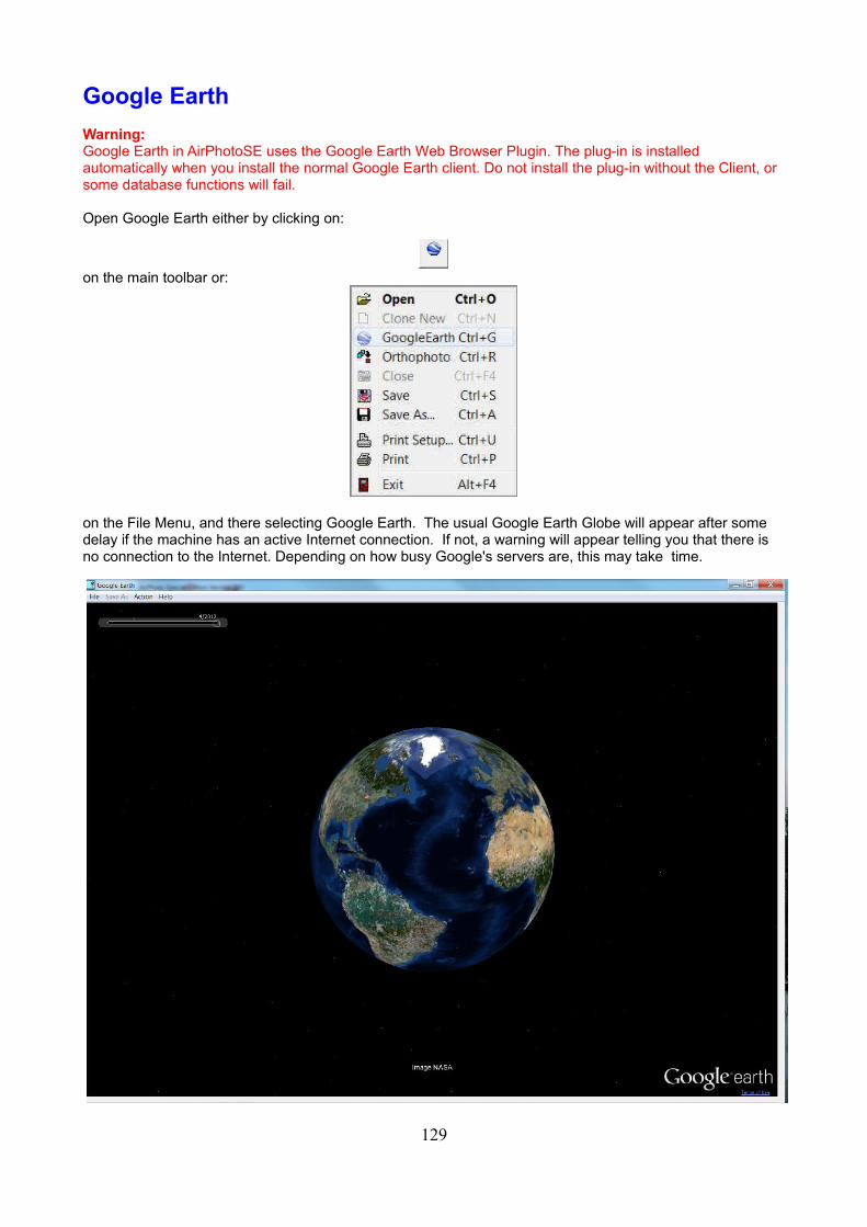
Google Earth

Warning:Google Earth in AirPhotoSE uses the Google Earth Web Browser Plugin. The plug-in is installed automatically when you install the normal Google Earth client. Do not install the plug-in without the Client, or some database functions will fail.

Open Google Earth either by clicking on:

on the main toolbar or:

on the File Menu, and there selecting Google Earth. The usual Google Earth Globe will appear after some delay if the machine has an active Internet connection. If not, a warning will appear telling you that there is no connection to the Internet. Depending on how busy Google's servers are, this may take time.

129

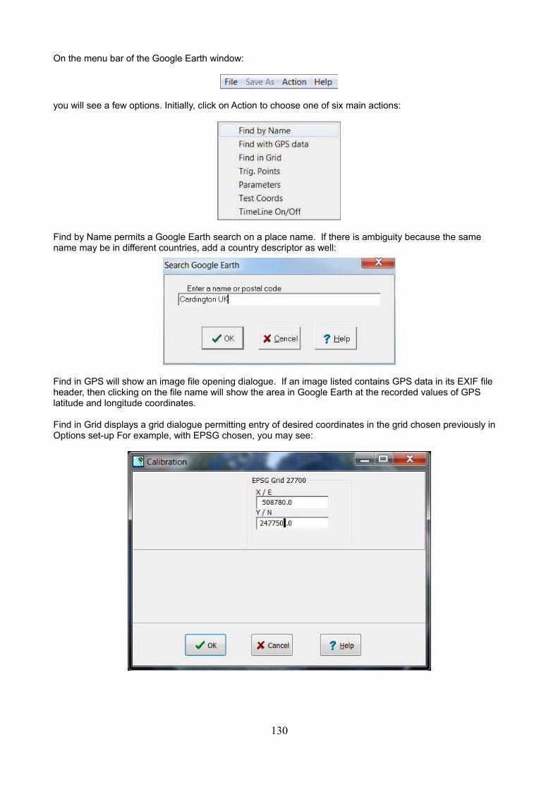
On the menu bar of the Google Earth window:

you will see a few options. Initially, click on Action to choose one of six main actions:

Find by Name permits a Google Earth search on a place name. If there is ambiguity because the same name may be in different countries, add a country descriptor as well:

Find in GPS will show an image file opening dialogue. If an image listed contains GPS data in its EXIF file header, then clicking on the file name will show the area in Google Earth at the recorded values of GPS latitude and longitude coordinates.

Find in Grid displays a grid dialogue permitting entry of desired coordinates in the grid chosen previously in Options set-up For example, with EPSG chosen, you may see:

130

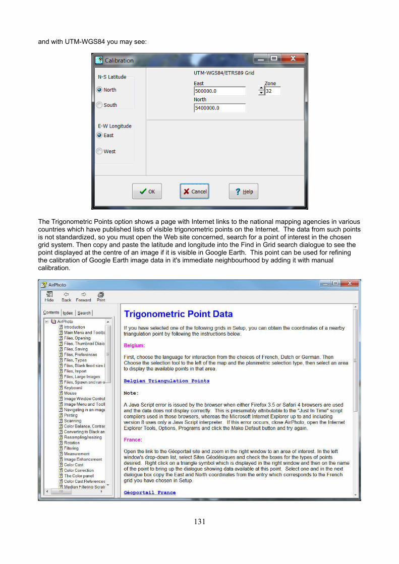
and with UTM-WGS84 you may see:

The Trigonometric Points option shows a page with Internet links to the national mapping agencies in variouscountries which have published lists of visible trigonometric points on the Internet. The data from such pointsis not standardized, so you must open the Web site concerned, search for a point of interest in the chosen grid system. Then copy and paste the latitude and longitude into the Find in Grid search dialogue to see the point displayed at the centre of an image if it is visible in Google Earth. This point can be used for refining the calibration of Google Earth image data in it's immediate neighbourhood by adding it with manual calibration.

131

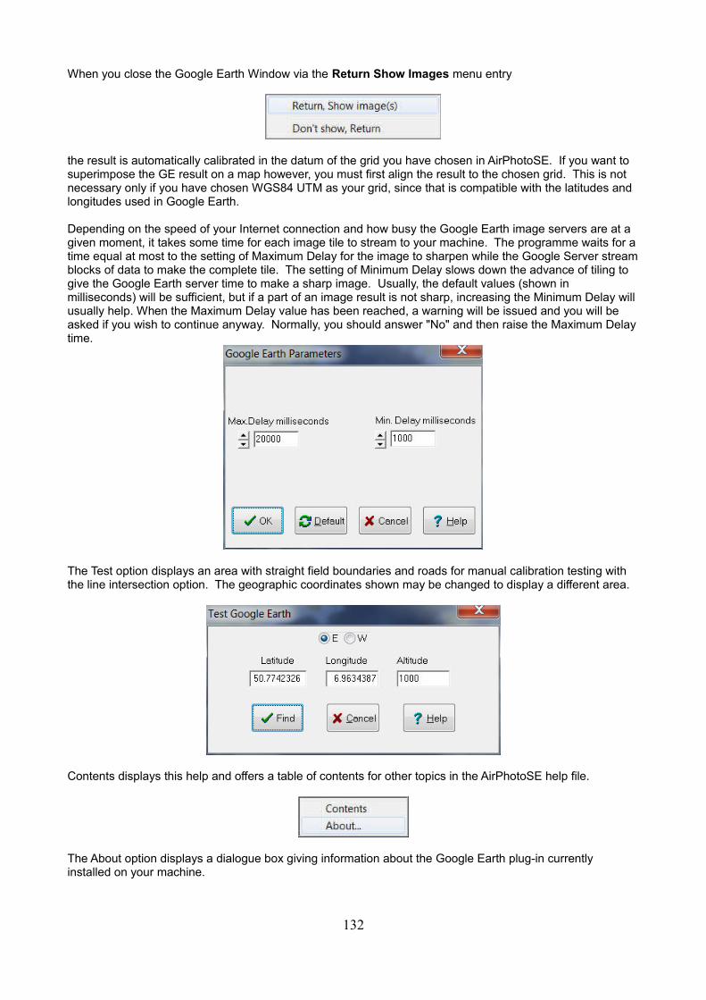
When you close the Google Earth Window via the Return Show Images menu entry

the result is automatically calibrated in the datum of the grid you have chosen in AirPhotoSE. If you want to superimpose the GE result on a map however, you must first align the result to the chosen grid. This is not necessary only if you have chosen WGS84 UTM as your grid, since that is compatible with the latitudes and longitudes used in Google Earth.

Depending on the speed of your Internet connection and how busy the Google Earth image servers are at a given moment, it takes some time for each image tile to stream to your machine. The programme waits for atime equal at most to the setting of Maximum Delay for the image to sharpen while the Google Server streamblocks of data to make the complete tile. The setting of Minimum Delay slows down the advance of tiling to give the Google Earth server time to make a sharp image. Usually, the default values (shown in milliseconds) will be sufficient, but if a part of an image result is not sharp, increasing the Minimum Delay will usually help. When the Maximum Delay value has been reached, a warning will be issued and you will be asked if you wish to continue anyway. Normally, you should answer "No" and then raise the Maximum Delaytime.

The Test option displays an area with straight field boundaries and roads for manual calibration testing with the line intersection option. The geographic coordinates shown may be changed to display a different area.

Contents displays this help and offers a table of contents for other topics in the AirPhotoSE help file.

The About option displays a dialogue box giving information about the Google Earth plug-in currently installed on your machine.

132

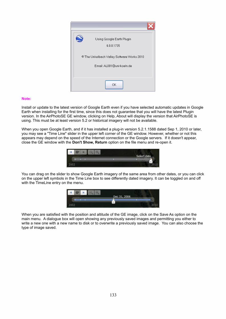
Note:

Install or update to the latest version of Google Earth even if you have selected automatic updates in Google Earth when installing for the first time, since this does not guarantee that you will have the latest Plugin version. In the AirPhotoSE GE window, clicking on Help, About will display the version that AirPhotoSE is using. This must be at least version 5.2 or historical imagery will not be available.

When you open Google Earth, and if it has installed a plug-in version 5.2.1.1588 dated Sep 1, 2010 or later, you may see a "Time Line" slider in the upper left corner of the GE window. However, whether or not this appears may depend on the speed of the Internet connection or the Google servers. If it doesn't appear, close the GE window with the Don't Show, Return option on the file menu and re-open it.

You can drag on the slider to show Google Earth imagery of the same area from other dates, or you can clickon the upper left symbols in the Time Line box to see differently dated imagery. It can be toggled on and off with the TimeLine entry on the menu.

When you are satisfied with the position and altitude of the GE image, click on the Save As option on the main menu. A dialogue box will open showing any previously saved images and permitting you either to write a new one with a new name to disk or to overwrite a previously saved image. You can also choose the type of image saved.

133

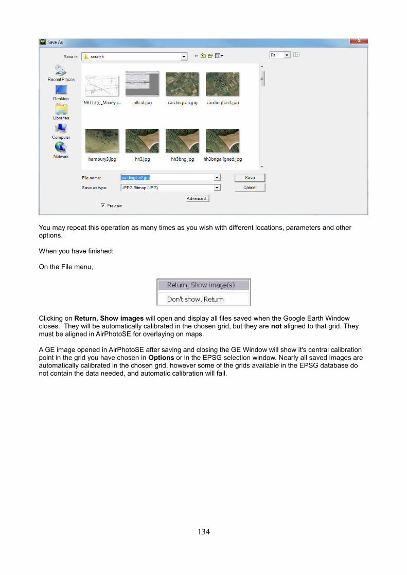
You may repeat this operation as many times as you wish with different locations, parameters and other options.

When you have finished:

On the File menu,

Clicking on Return, Show images will open and display all files saved when the Google Earth Window closes. They will be automatically calibrated in the chosen grid, but they are not aligned to that grid. They must be aligned in AirPhotoSE for overlaying on maps.

A GE image opened in AirPhotoSE after saving and closing the GE Window will show it's central calibration point in the grid you have chosen in Options or in the EPSG selection window. Nearly all saved images are automatically calibrated in the chosen grid, however some of the grids available in the EPSG database do not contain the data needed, and automatic calibration will fail.

134

135

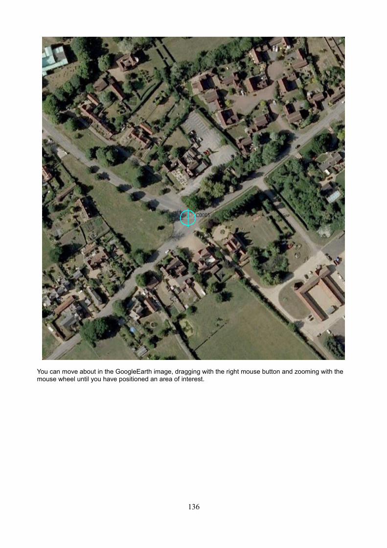
You can move about in the GoogleEarth image, dragging with the right mouse button and zooming with the mouse wheel until you have positioned an area of interest.

136

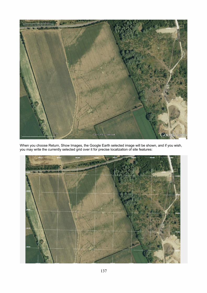
When you choose Return, Show Images, the Google Earth selected image will be shown, and if you wish, you may write the currently selected grid over it for precise localization of site features:

137

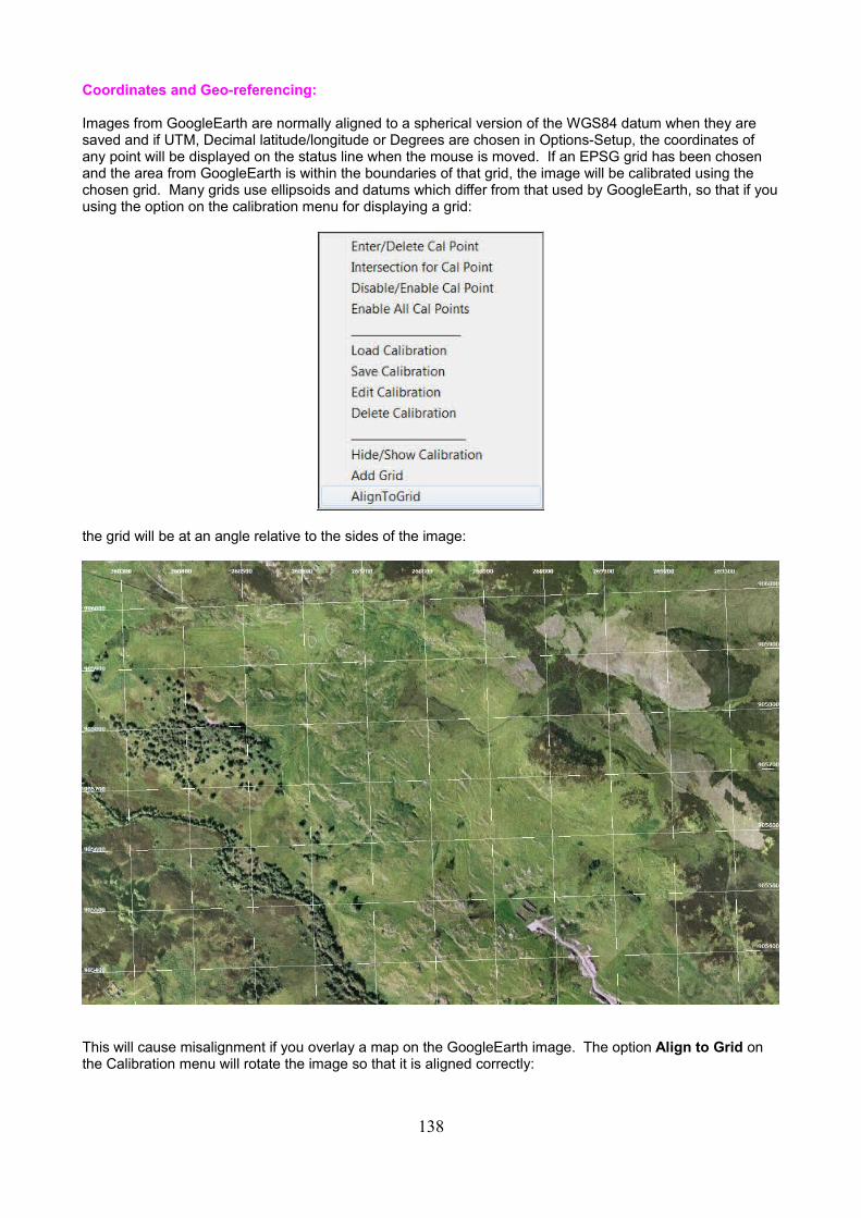
Coordinates and Geo-referencing:

Images from GoogleEarth are normally aligned to a spherical version of the WGS84 datum when they are saved and if UTM, Decimal latitude/longitude or Degrees are chosen in Options-Setup, the coordinates of any point will be displayed on the status line when the mouse is moved. If an EPSG grid has been chosen and the area from GoogleEarth is within the boundaries of that grid, the image will be calibrated using the chosen grid. Many grids use ellipsoids and datums which differ from that used by GoogleEarth, so that if youusing the option on the calibration menu for displaying a grid:

the grid will be at an angle relative to the sides of the image:

This will cause misalignment if you overlay a map on the GoogleEarth image. The option Align to Grid on the Calibration menu will rotate the image so that it is aligned correctly:

138

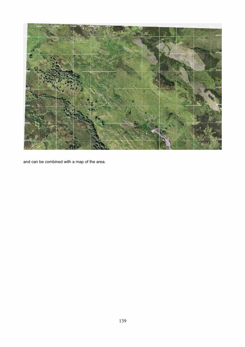
and can be combined with a map of the area.

139

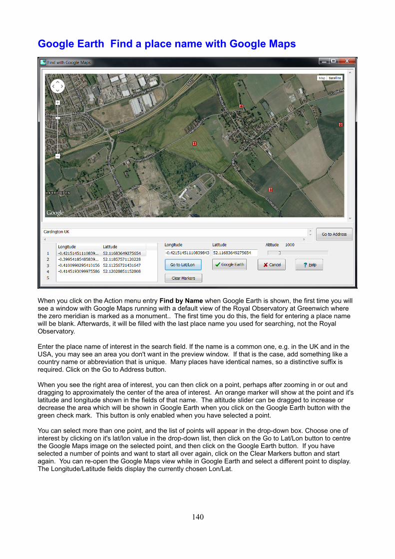
Google Earth Find a place name with Google Maps

When you click on the Action menu entry Find by Name when Google Earth is shown, the first time you will see a window with Google Maps running with a default view of the Royal Observatory at Greenwich where the zero meridian is marked as a monument.. The first time you do this, the field for entering a place name will be blank. Afterwards, it will be filled with the last place name you used for searching, not the Royal Observatory.

Enter the place name of interest in the search field. If the name is a common one, e.g. in the UK and in the USA, you may see an area you don't want in the preview window. If that is the case, add something like a country name or abbreviation that is unique. Many places have identical names, so a distinctive suffix is required. Click on the Go to Address button.

When you see the right area of interest, you can then click on a point, perhaps after zooming in or out and dragging to approximately the center of the area of interest. An orange marker will show at the point and it's latitude and longitude shown in the fields of that name. The altitude slider can be dragged to increase or decrease the area which will be shown in Google Earth when you click on the Google Earth button with the green check mark. This button is only enabled when you have selected a point.

You can select more than one point, and the list of points will appear in the drop-down box. Choose one of interest by clicking on it's lat/lon value in the drop-down list, then click on the Go to Lat/Lon button to centre the Google Maps image on the selected point, and then click on the Google Earth button. If you have selected a number of points and want to start all over again, click on the Clear Markers button and start again. You can re-open the Google Maps view while in Google Earth and select a different point to display. The Longitude/Latitude fields display the currently chosen Lon/Lat.

140

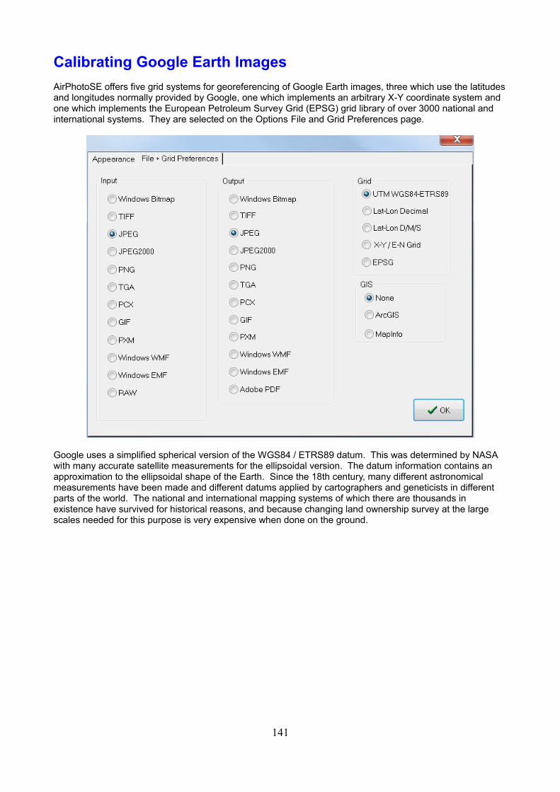
Calibrating Google Earth Images

AirPhotoSE offers five grid systems for georeferencing of Google Earth images, three which use the latitudesand longitudes normally provided by Google, one which implements an arbitrary X-Y coordinate system and one which implements the European Petroleum Survey Grid (EPSG) grid library of over 3000 national and international systems. They are selected on the Options File and Grid Preferences page.

Google uses a simplified spherical version of the WGS84 / ETRS89 datum. This was determined by NASA with many accurate satellite measurements for the ellipsoidal version. The datum information contains an approximation to the ellipsoidal shape of the Earth. Since the 18th century, many different astronomical measurements have been made and different datums applied by cartographers and geneticists in different parts of the world. The national and international mapping systems of which there are thousands in existence have survived for historical reasons, and because changing land ownership survey at the large scales needed for this purpose is very expensive when done on the ground.

141

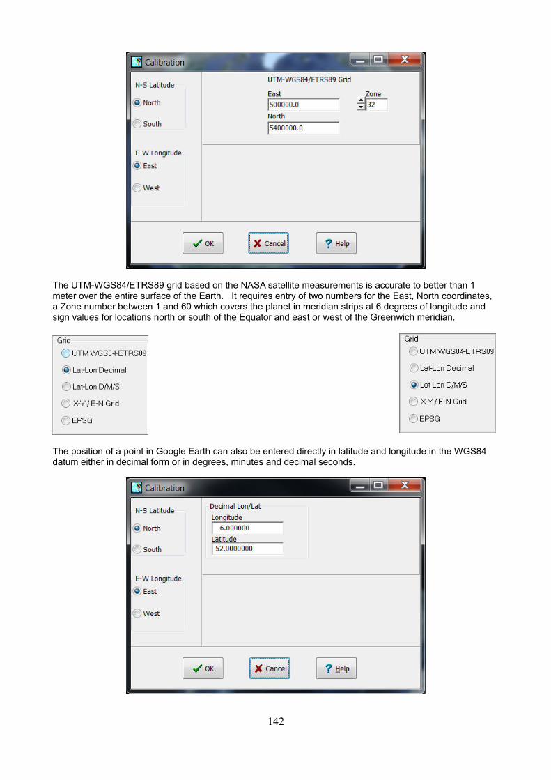
The UTM-WGS84/ETRS89 grid based on the NASA satellite measurements is accurate to better than 1 meter over the entire surface of the Earth. It requires entry of two numbers for the East, North coordinates, a Zone number between 1 and 60 which covers the planet in meridian strips at 6 degrees of longitude and sign values for locations north or south of the Equator and east or west of the Greenwich meridian.

The position of a point in Google Earth can also be entered directly in latitude and longitude in the WGS84 datum either in decimal form or in degrees, minutes and decimal seconds.

142

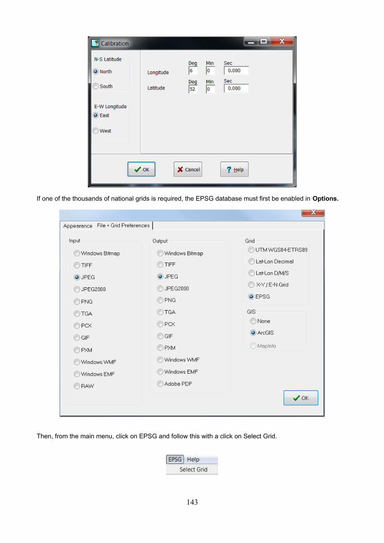
If one of the thousands of national grids is required, the EPSG database must first be enabled in Options.

Then, from the main menu, click on EPSG and follow this with a click on Select Grid.

143

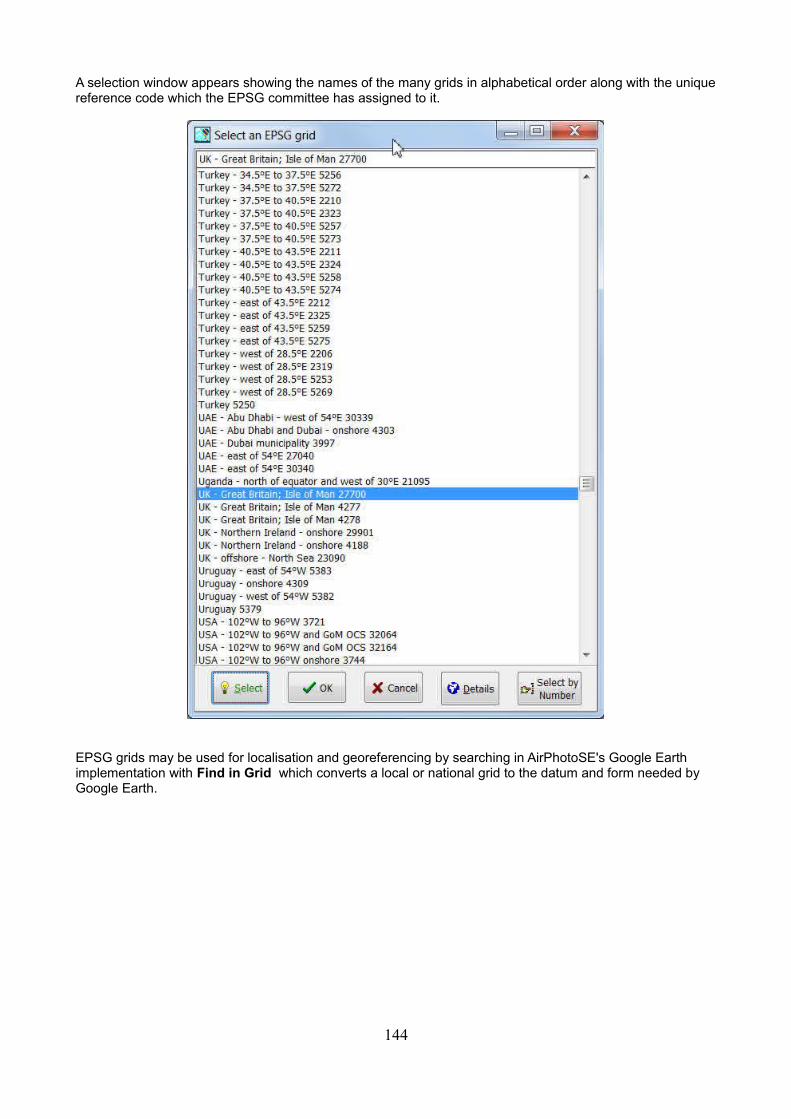
A selection window appears showing the names of the many grids in alphabetical order along with the uniquereference code which the EPSG committee has assigned to it.

EPSG grids may be used for localisation and georeferencing by searching in AirPhotoSE's Google Earth implementation with Find in Grid which converts a local or national grid to the datum and form needed by Google Earth.

144

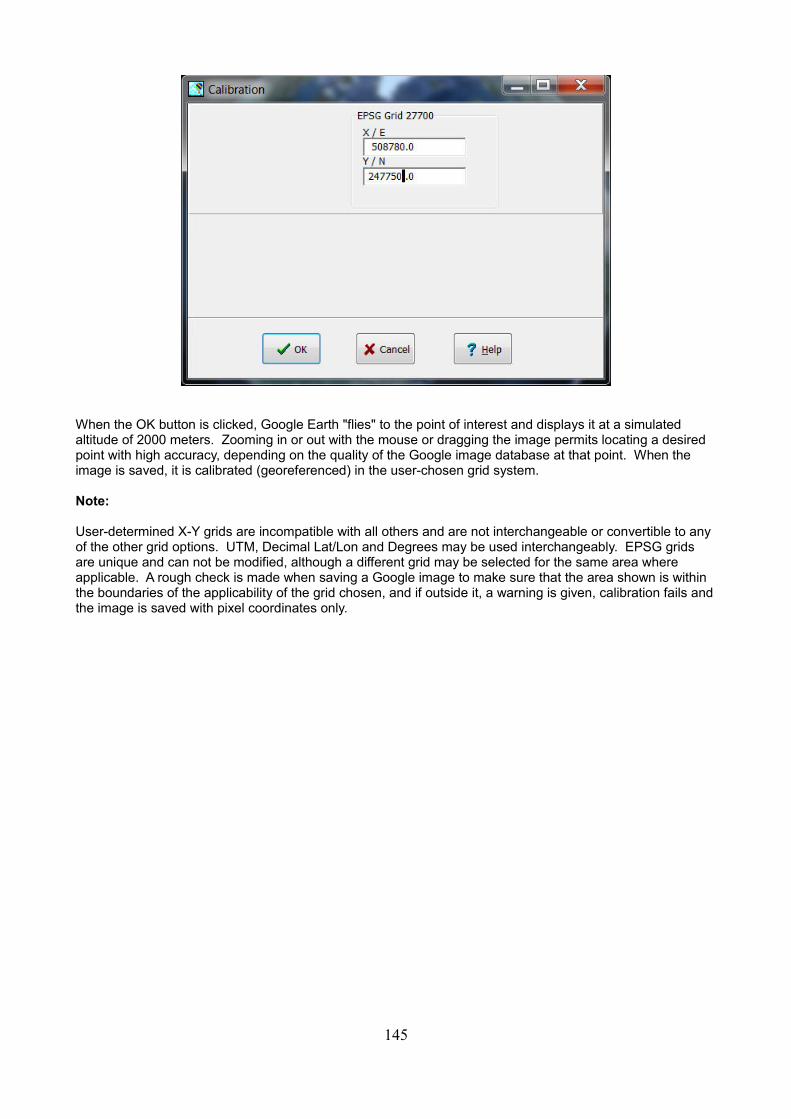
When the OK button is clicked, Google Earth "flies" to the point of interest and displays it at a simulated altitude of 2000 meters. Zooming in or out with the mouse or dragging the image permits locating a desired point with high accuracy, depending on the quality of the Google image database at that point. When the image is saved, it is calibrated (georeferenced) in the user-chosen grid system.

Note:

User-determined X-Y grids are incompatible with all others and are not interchangeable or convertible to any of the other grid options. UTM, Decimal Lat/Lon and Degrees may be used interchangeably. EPSG grids are unique and can not be modified, although a different grid may be selected for the same area where applicable. A rough check is made when saving a Google image to make sure that the area shown is within the boundaries of the applicability of the grid chosen, and if outside it, a warning is given, calibration fails andthe image is saved with pixel coordinates only.

145

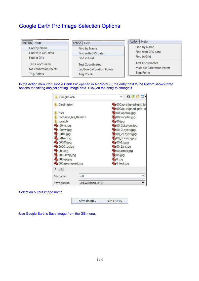
Google Earth Pro Image Selection Options

In the Action menu for Google Earth Pro opened in AirPhotoSE, the entry next to the bottom shows three options for saving and calibrating image data. Click on the entry to change it.

Select an output image name

Use Google Earth's Save Image from the GE menu.

146

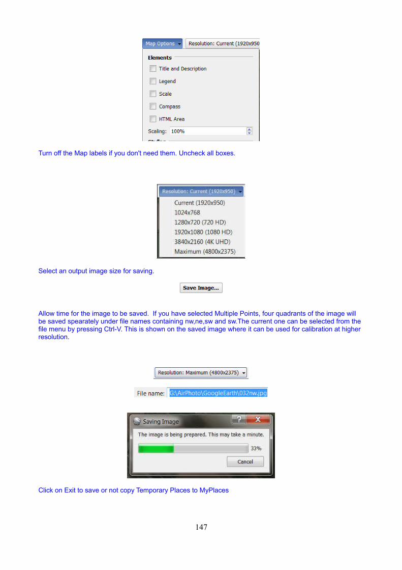
Turn off the Map labels if you don't need them. Uncheck all boxes.

Select an output image size for saving.

Allow time for the image to be saved. If you have selected Multiple Points, four quadrants of the image will be saved spearately under file names containing nw,ne,sw and sw.The current one can be selected from the file menu by pressing Ctrl-V. This is shown on the saved image where it can be used for calibration at higher resolution.

Click on Exit to save or not copy Temporary Places to MyPlaces

147

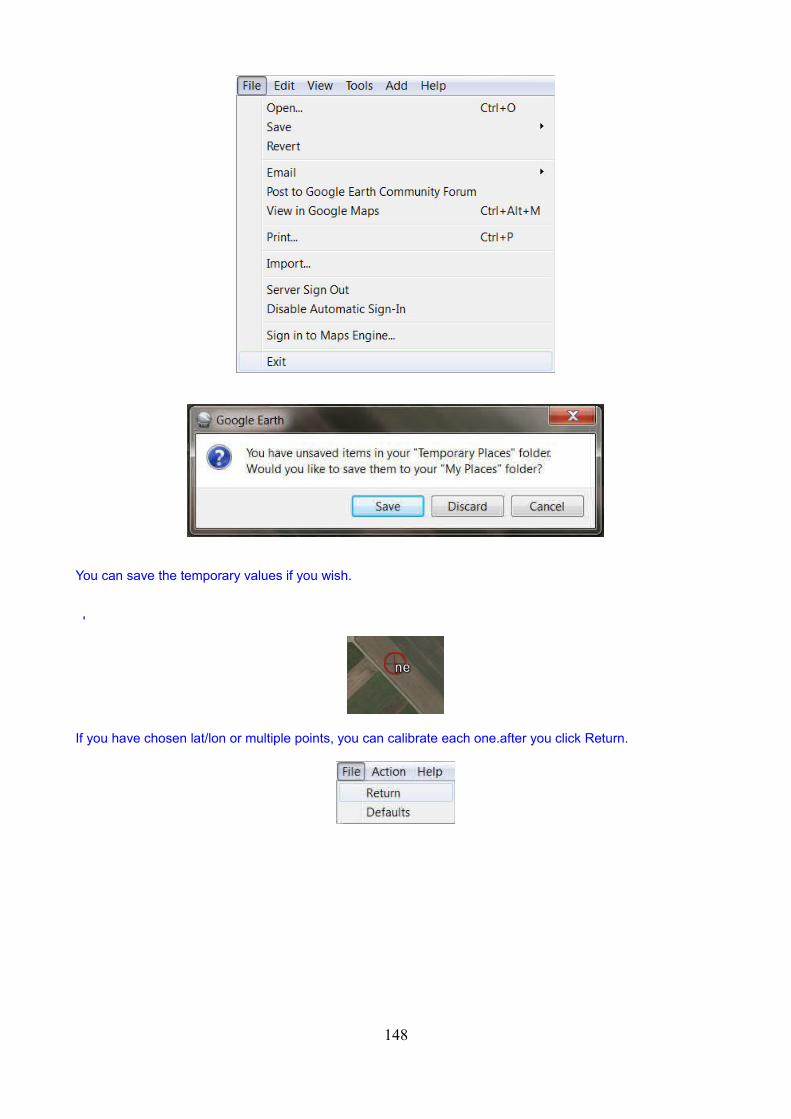
You can save the temporary values if you wish.

'

If you have chosen lat/lon or multiple points, you can calibrate each one.after you click Return.

148

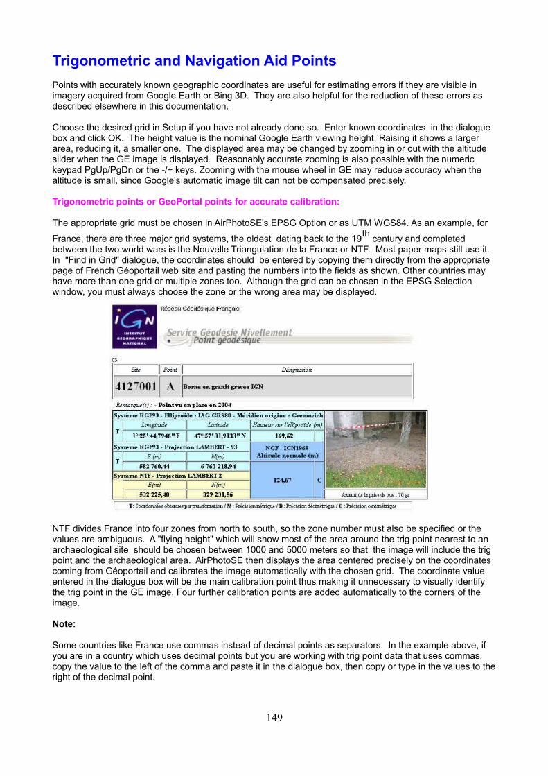
Trigonometric and Navigation Aid Points

Points with accurately known geographic coordinates are useful for estimating errors if they are visible in imagery acquired from Google Earth or Bing 3D. They are also helpful for the reduction of these errors as described elsewhere in this documentation.

Choose the desired grid in Setup if you have not already done so. Enter known coordinates in the dialogue box and click OK. The height value is the nominal Google Earth viewing height. Raising it shows a larger area, reducing it, a smaller one. The displayed area may be changed by zooming in or out with the altitude slider when the GE image is displayed. Reasonably accurate zooming is also possible with the numeric keypad PgUp/PgDn or the -/+ keys. Zooming with the mouse wheel in GE may reduce accuracy when the altitude is small, since Google's automatic image tilt can not be compensated precisely.

Trigonometric points or GeoPortal points for accurate calibration:

The appropriate grid must be chosen in AirPhotoSE's EPSG Option or as UTM WGS84. As an example, for

France, there are three major grid systems, the oldest dating back to the 19th

century and completed between the two world wars is the Nouvelle Triangulation de la France or NTF. Most paper maps still use it. In "Find in Grid" dialogue, the coordinates should be entered by copying them directly from the appropriate page of French Géoportail web site and pasting the numbers into the fields as shown. Other countries may have more than one grid or multiple zones too. Although the grid can be chosen in the EPSG Selection window, you must always choose the zone or the wrong area may be displayed.

NTF divides France into four zones from north to south, so the zone number must also be specified or the values are ambiguous. A "flying height" which will show most of the area around the trig point nearest to an archaeological site should be chosen between 1000 and 5000 meters so that the image will include the trig point and the archaeological area. AirPhotoSE then displays the area centered precisely on the coordinates coming from Géoportail and calibrates the image automatically with the chosen grid. The coordinate value entered in the dialogue box will be the main calibration point thus making it unnecessary to visually identify the trig point in the GE image. Four further calibration points are added automatically to the corners of the image.

Note:

Some countries like France use commas instead of decimal points as separators. In the example above, if you are in a country which uses decimal points but you are working with trig point data that uses commas, copy the value to the left of the comma and paste it in the dialogue box, then copy or type in the values to theright of the decimal point.

149

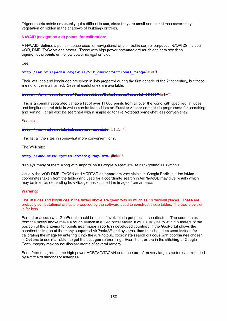
Trigonometric points are usually quite difficult to see, since they are small and sometimes covered by vegetation or hidden in the shadows of buildings or trees.

NAVAID (navigation aid) points for calibration:

A NAVAID defines a point in space used for navigational and air traffic control purposes. NAVAIDS include VOR, DME, TACANs and others. Those with high power antennae are much easier to see than trigonometric points or the low power navigation aids.

See:

http://en.wikipedia.org/wiki/VHF_omnidirectional_range{link=*!

Their latitudes and longitudes are given in lists prepared during the first decade of the 21st century, but theseare no longer maintained. Several useful ones are available:

https://www.google.com/fusiontables/DataSource?dsrcid=934957{link=*!

This is a comma separated variable list of over 11,000 points from all over the world with specified latitudes and longitudes and details which can be loaded into an Excel or Access compatible programme for searchingand sorting. It can also be searched with a simple editor like Notepad somewhat less conveniently..

See also:

http://www.airportdatabase.net/navaids{link=*!

This list all the sites in somewhat more convenient form.

The Web site:

http://www.ourairports.com/big-map.html{link=*!

displays many of them along with airports on a Google Maps/Satellite background as symbols.

Usually the VOR-DME, TACAN and VORTAC antennae are very visible in Google Earth, but the lat/lon coordinates taken from the tables and used for a coordinate search in AirPhotoSE may give results which may be in error, depending how Google has stitched the images from an area.

Warning:

The latitudes and longitudes in the tables above are given with as much as 18 decimal places. These are probably computational artifacts produced by the software used to construct those tables. The true precision is far less.

For better accuracy, a GeoPortal should be used if available to get precise coordinates. The coordinates from the tables above make a rough search in a GeoPortal easier. It will usually be to within 5 meters of the position of the antenna for points near major airports in developed countries. If the GeoPortal shows the coordinates in one of the many supported AirPhotoSE grid systems, then this should be used instead for calibrating the image by entering it into the AirPhotoSE coordinate search dialogue with coordinates chosen in Options to decimal lat/lon to get the best geo-referencing. Even then, errors in the stitching of Google Earth imagery may cause displacements of several meters.

Seen from the ground, the high power VORTAC/TACAN antennae are often very large structures surroundedby a circle of secondary antennae:

150

151

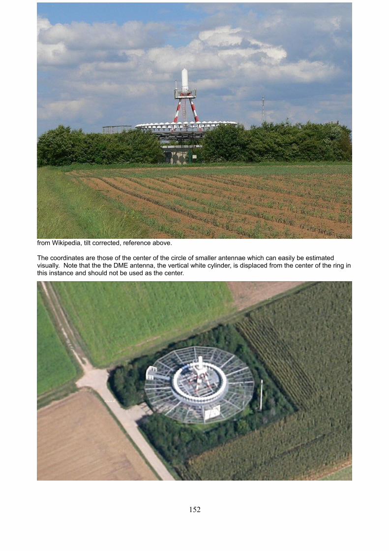
from Wikipedia, tilt corrected, reference above.

The coordinates are those of the center of the circle of smaller antennae which can easily be estimated visually. Note that the the DME antenna, the vertical white cylinder, is displaced from the center of the ring inthis instance and should not be used as the center.

152

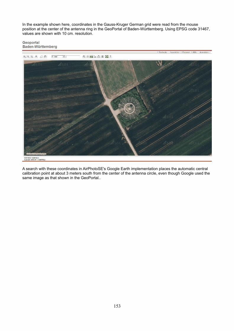
In the example shown here, coordinates in the Gauss-Kruger German grid were read from the mouse position at the center of the antenna ring in the GeoPortal of Baden-Württemberg. Using EPSG code 31467, values are shown with 10 cm. resolution.

A search with these coordinates in AirPhotoSE's Google Earth implementation places the automatic central calibration point at about 3 meters south from the center of the antenna circle, even though Google used the same image as that shown in the GeoPortal..

153

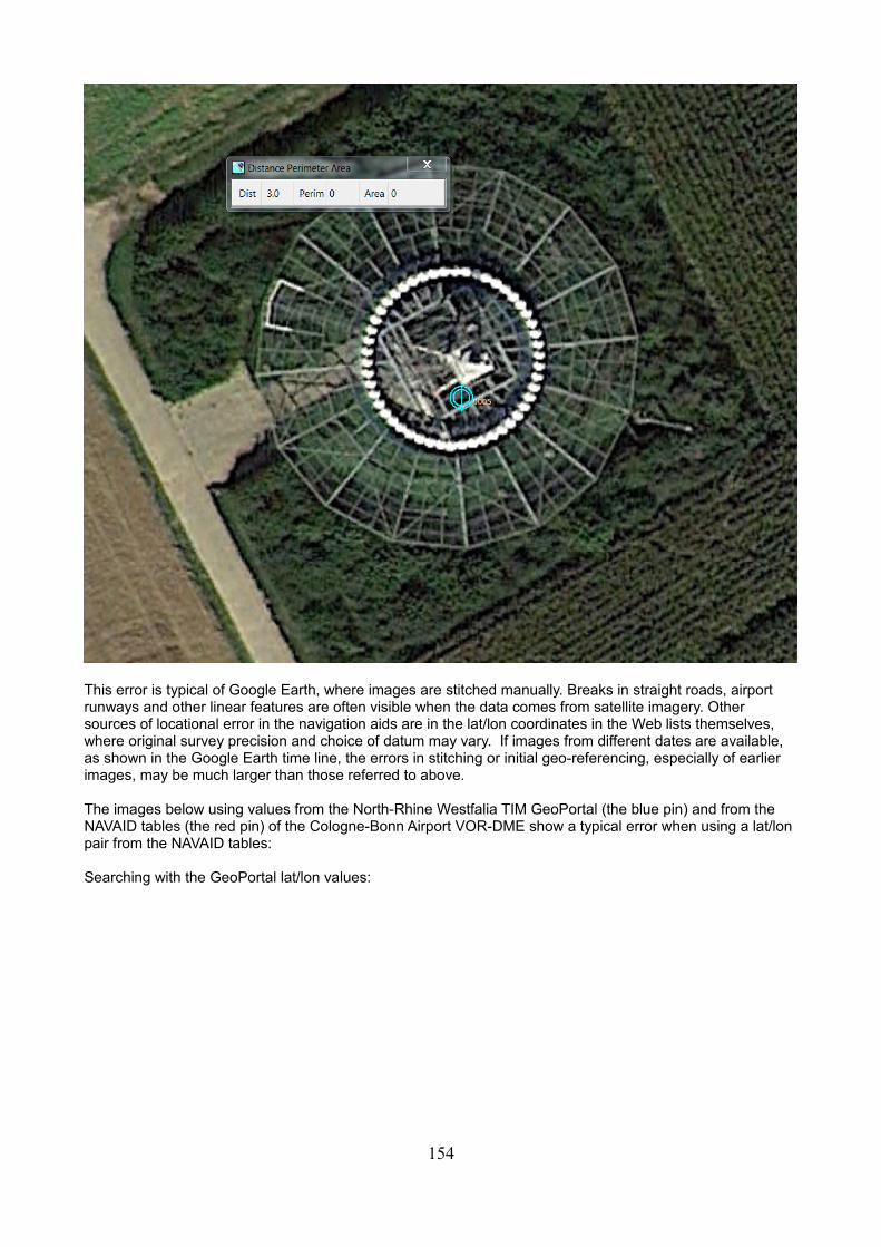
This error is typical of Google Earth, where images are stitched manually. Breaks in straight roads, airport runways and other linear features are often visible when the data comes from satellite imagery. Other sources of locational error in the navigation aids are in the lat/lon coordinates in the Web lists themselves, where original survey precision and choice of datum may vary. If images from different dates are available, as shown in the Google Earth time line, the errors in stitching or initial geo-referencing, especially of earlier images, may be much larger than those referred to above.

The images below using values from the North-Rhine Westfalia TIM GeoPortal (the blue pin) and from the NAVAID tables (the red pin) of the Cologne-Bonn Airport VOR-DME show a typical error when using a lat/lon pair from the NAVAID tables:

Searching with the GeoPortal lat/lon values:

154

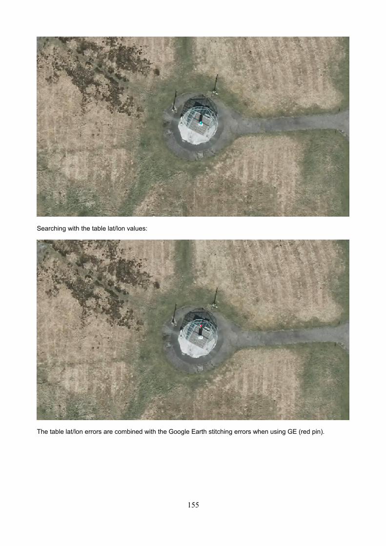
Searching with the table lat/lon values:

The table lat/lon errors are combined with the Google Earth stitching errors when using GE (red pin).

155

Google Earth: Improving Accuracy

Google Earth images do not have photogrammetric accuracy. The error at the center of an image found by entering a latitude/longitude value in the stand-alone version of Google Earth and the correct position of that point may differ by more than ten meters even in areas of high resolution. If you know the latitude and longitude of a trigonometric or other precisely known point which is visible in GE, you can confirm this by entering the lat/lon in the Google search box and examining where GE puts its center point relative to the visible trigonometric point.

In AirPhotoSE, use the Find in Coordinates for searching in GE with accuracy. Do not use any other search option, and do not zoom into the image with mouse wheel.

Any known point used for searching in the Find by Coordinates search dialogue may be used, but accuracy differs.

1) Differential GPS or RTK measurement in the field of a highly visible point in Google Earth with appropriate hardware:

http://en.wikipedia.org/wiki/Real_Time_Kinematic

In Europe see:

http://www.essp-sas.eu/downloads/omsopvd/edas_sdd_in_force.pdf

2) A GE-visible trigonometric point with known coordinates,.

In the UK, you can obtain complete lists of latitudes and longitudes for more than 6000 trigonometric point pillars placed by the Ordnance Survey between 1936 and 1962 from:

http://www.haroldstreet.org.uk/waypoints.php?hill=trigpoints

Unfortunately, these points are no longer maintained and many are not visible in Google Earth, but if one is visible in your immediate area of interest and in the same flight imagery,you can use the BNG coordinates EPSG 27700 in the Find in Grid dialog box of AirPhotoSE. This requires the use of the full OSGB coordinates in Easting and Northing. The map lettering scheme of British National Grid and the Irish RepublicGrid must be converted to the long format.

Lists of trig points are sometimes available elsewhere, but many countries require payment for using them. The UK data gives a good idea of general GE accuracy under favourable conditions.

3) If you know the coordinates in the preferred local grid of any visible point from a GeoPortal site, you can also improve the accuracy of GE calibration in AirPhotoSE considerably by using the coordinates from the mouse position if the GeoPortal displays these to meter precision or better.

4) If nearby, the lat/lon coordinates of a navigation aid used for searching as described in the previous section of this documentation The best points are close to major airports, and usually these areas may not be entered in a low-flying aircraft. Be aware that the accuracy of these values is questionable outside of highly developed countries.

Warning:

Google imaging uses the Plate Carée projection which is a transverse cylindrical Mercator projection to a sphere and not to an ellipsoid. The non-conformal Plate Carée projection is inherently distorted unlike most large scale maps which use a conformal projection.. For areas smaller than about 2 kilometers square, the error is usually of the order of a meter or two and can usually be neglected. It becomes significant for larger areas, so try to zoom the Google image to enclose the smallest possible area required. AirPhoto does not correct for distortion in a Google Earth image but it does transform the calibration points at the corners and center of the image to the ellipsoid of the UTM grid before applying a datum transformation to the chosen national or international grid.

156

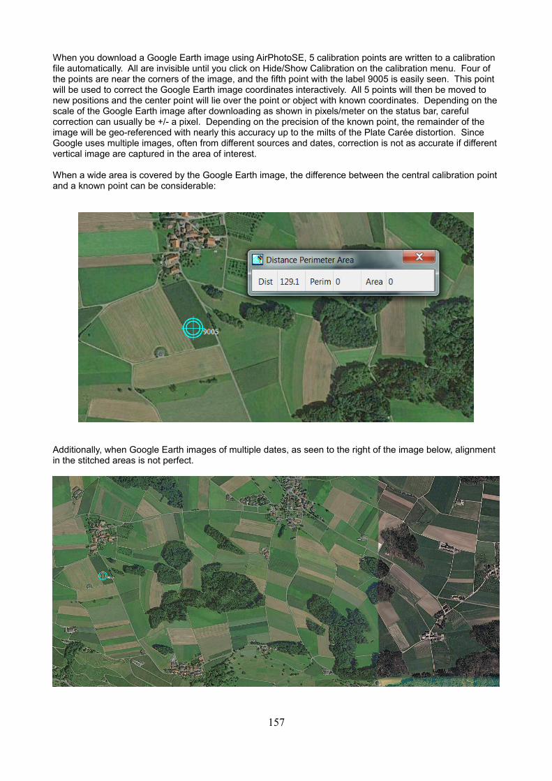
When you download a Google Earth image using AirPhotoSE, 5 calibration points are written to a calibration file automatically. All are invisible until you click on Hide/Show Calibration on the calibration menu. Four of the points are near the corners of the image, and the fifth point with the label 9005 is easily seen. This point will be used to correct the Google Earth image coordinates interactively. All 5 points will then be moved to new positions and the center point will lie over the point or object with known coordinates. Depending on thescale of the Google Earth image after downloading as shown in pixels/meter on the status bar, careful correction can usually be +/- a pixel. Depending on the precision of the known point, the remainder of the image will be geo-referenced with nearly this accuracy up to the milts of the Plate Carée distortion. Since Google uses multiple images, often from different sources and dates, correction is not as accurate if differentvertical image are captured in the area of interest.

When a wide area is covered by the Google Earth image, the difference between the central calibration pointand a known point can be considerable:

Additionally, when Google Earth images of multiple dates, as seen to the right of the image below, alignment in the stitched areas is not perfect.

157

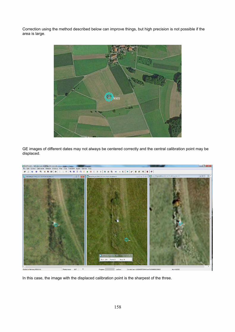
Correction using the method described below can improve things, but high precision is not possible if the area is large.

GE images of different dates may not always be centered correctly and the central calibration point may be displaced.

In this case, the image with the displaced calibration point is the sharpest of the three.

158

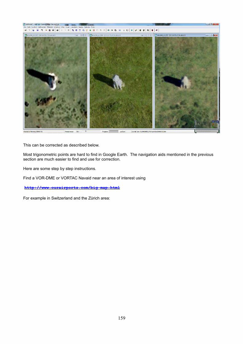
This can be corrected as described below.

Most trigonometric points are hard to find in Google Earth. The navigation aids mentioned in the previous section are much easier to find and use for correction.

Here are some step by step instructions.

Find a VOR-DME or VORTAC Navaid near an area of interest using

http://www.ourairports.com/big-map.html

For example in Switzerland and the Zürich area:

159

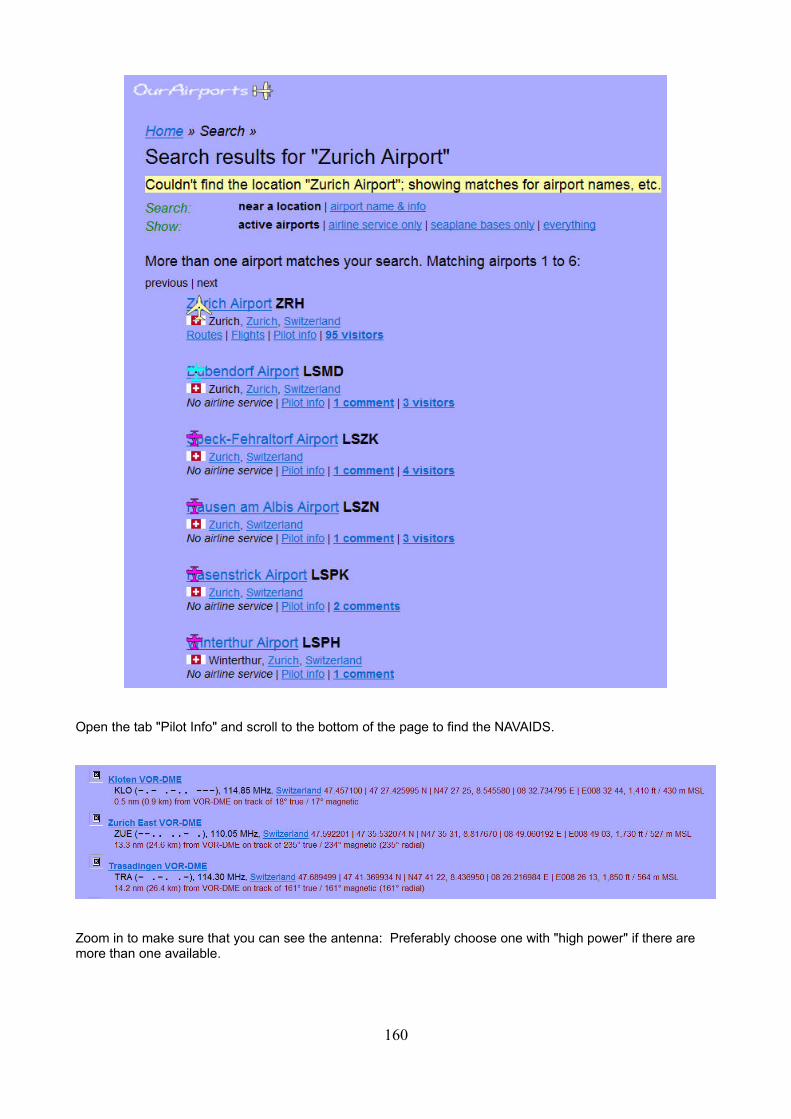
Open the tab "Pilot Info" and scroll to the bottom of the page to find the NAVAIDS.

Zoom in to make sure that you can see the antenna: Preferably choose one with "high power" if there are more than one available.

160

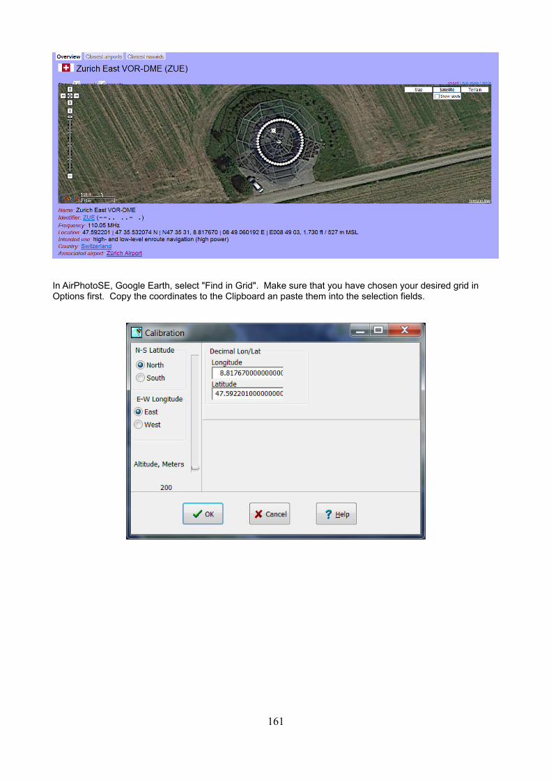
In AirPhotoSE, Google Earth, select "Find in Grid". Make sure that you have chosen your desired grid in Options first. Copy the coordinates to the Clipboard an paste them into the selection fields.

161

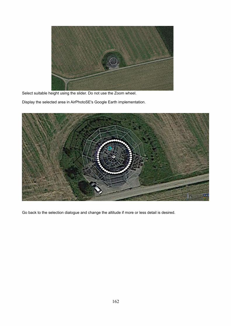
Select suitable height using the slider. Do not use the Zoom wheel.

Display the selected area in AirPhotoSE's Google Earth implementation.

Go back to the selection dialogue and change the altitude if more or less detail is desired.

162

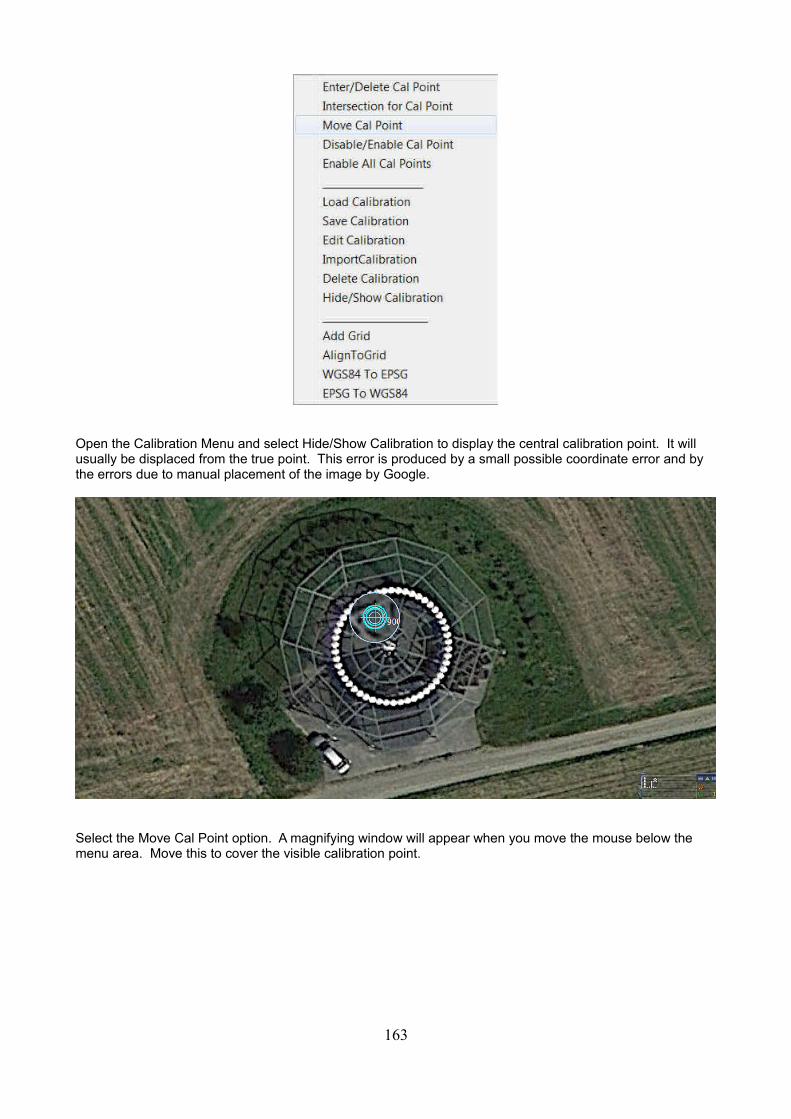
Open the Calibration Menu and select Hide/Show Calibration to display the central calibration point. It will usually be displaced from the true point. This error is produced by a small possible coordinate error and by the errors due to manual placement of the image by Google.

Select the Move Cal Point option. A magnifying window will appear when you move the mouse below the menu area. Move this to cover the visible calibration point.

163

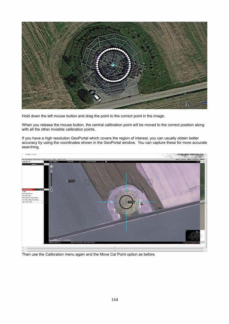
Hold down the left mouse button and drag the point to the correct point in the image.

When you release the mouse button, the central calibration point will be moved to the correct position along with all the other invisible calibration points.

If you have a high resolution GeoPortal which covers the region of interest, you can usually obtain better accuracy by using the coordinates shown in the GeoPortal window. You can capture these for more accuratesearching.

Then use the Calibration menu again and the Move Cal Point option as before.

164

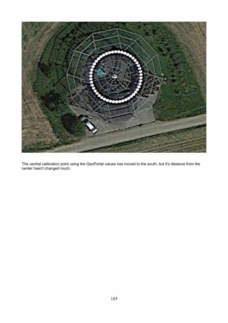
The central calibration point using the GeoPortal values has moved to the south, but it's distance from the center hasn't changed much.

165

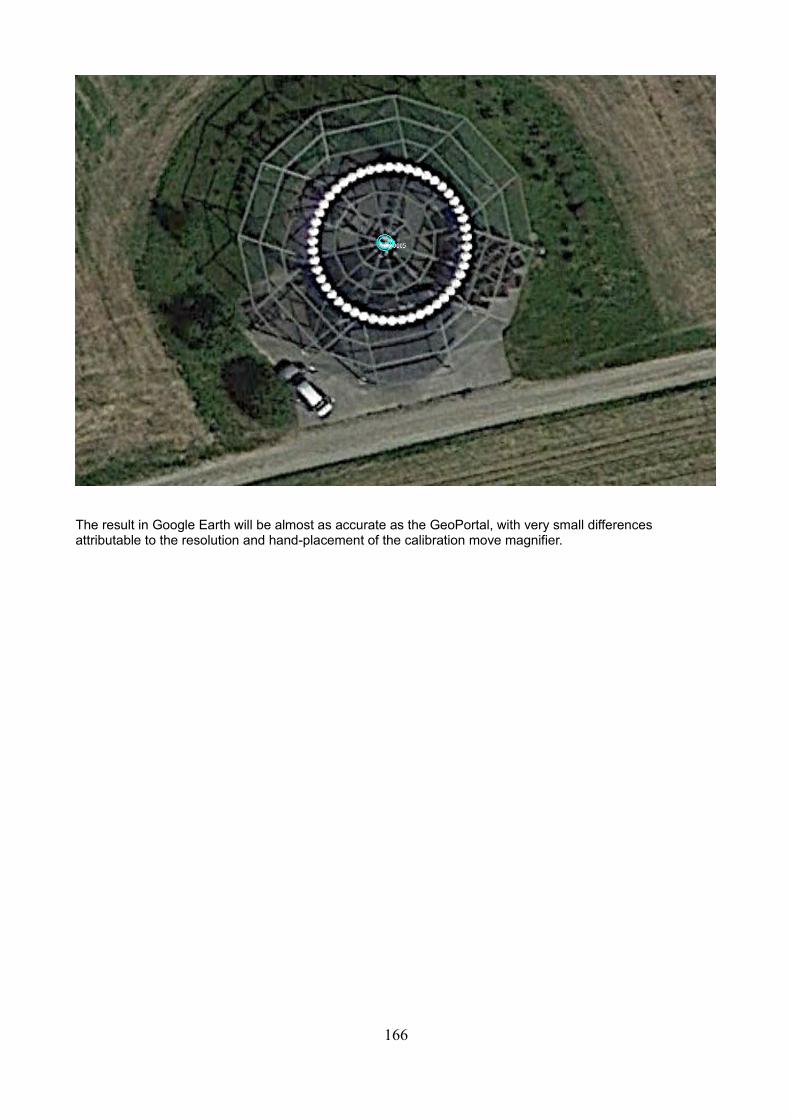
The result in Google Earth will be almost as accurate as the GeoPortal, with very small differences attributable to the resolution and hand-placement of the calibration move magnifier.

166

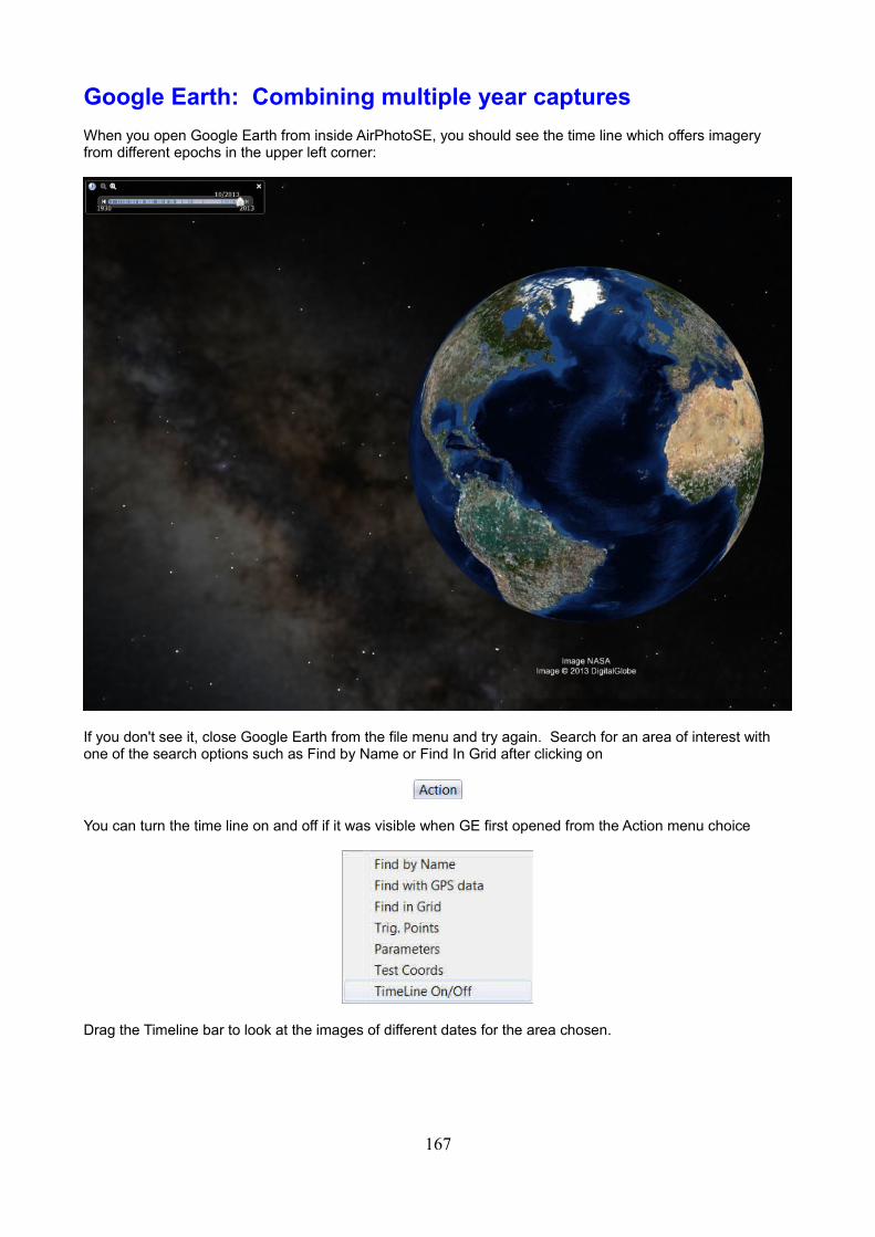
Google Earth: Combining multiple year captures

When you open Google Earth from inside AirPhotoSE, you should see the time line which offers imagery from different epochs in the upper left corner:

If you don't see it, close Google Earth from the file menu and try again. Search for an area of interest with one of the search options such as Find by Name or Find In Grid after clicking on

You can turn the time line on and off if it was visible when GE first opened from the Action menu choice

Drag the Timeline bar to look at the images of different dates for the area chosen.

167

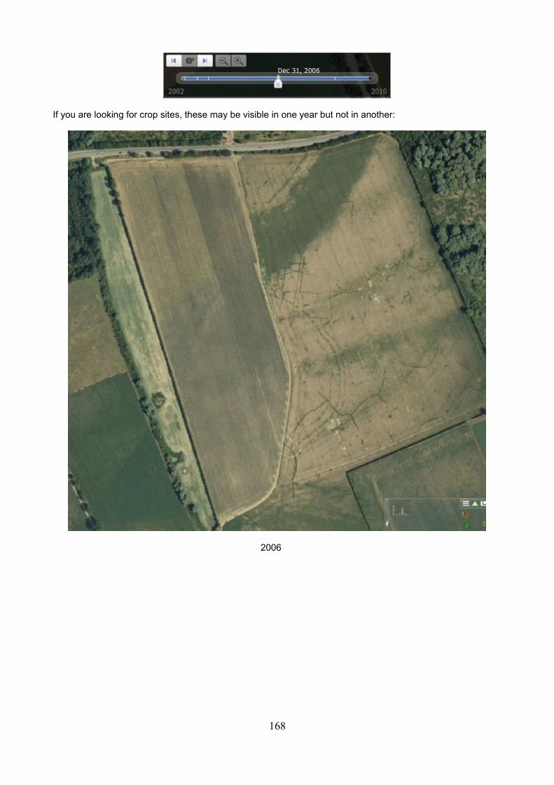
If you are looking for crop sites, these may be visible in one year but not in another:

2006

168

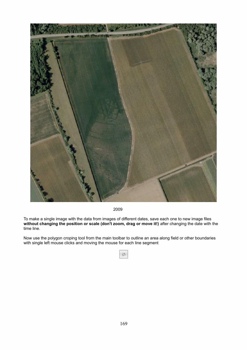
2009

To make a single image with the data from images of different dates, save each one to new image files without changing the position or scale (don't zoom, drag or move it!) after changing the date with the time line.

Now use the polygon croping tool from the main toolbar to outline an area along field or other boundaries with single left mouse clicks and moving the mouse for each line segment

169

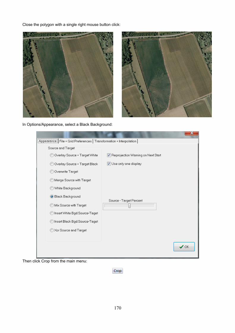
Close the polygon with a single right mouse button click:

In Options/Appearance, select a Black Background:

Then click Crop from the main menu:

170

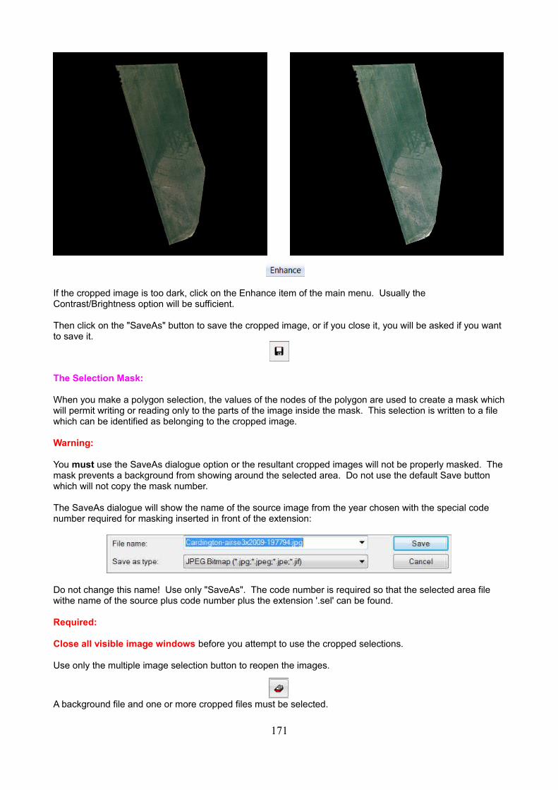
If the cropped image is too dark, click on the Enhance item of the main menu. Usually the Contrast/Brightness option will be sufficient.

Then click on the "SaveAs" button to save the cropped image, or if you close it, you will be asked if you want to save it.

The Selection Mask:

When you make a polygon selection, the values of the nodes of the polygon are used to create a mask whichwill permit writing or reading only to the parts of the image inside the mask. This selection is written to a file which can be identified as belonging to the cropped image.

Warning:

You must use the SaveAs dialogue option or the resultant cropped images will not be properly masked. Themask prevents a background from showing around the selected area. Do not use the default Save button which will not copy the mask number.

The SaveAs dialogue will show the name of the source image from the year chosen with the special code number required for masking inserted in front of the extension:

Do not change this name! Use only "SaveAs". The code number is required so that the selected area file withe name of the source plus code number plus the extension '.sel' can be found.

Required:

Close all visible image windows before you attempt to use the cropped selections.

Use only the multiple image selection button to reopen the images.

A background file and one or more cropped files must be selected.

171

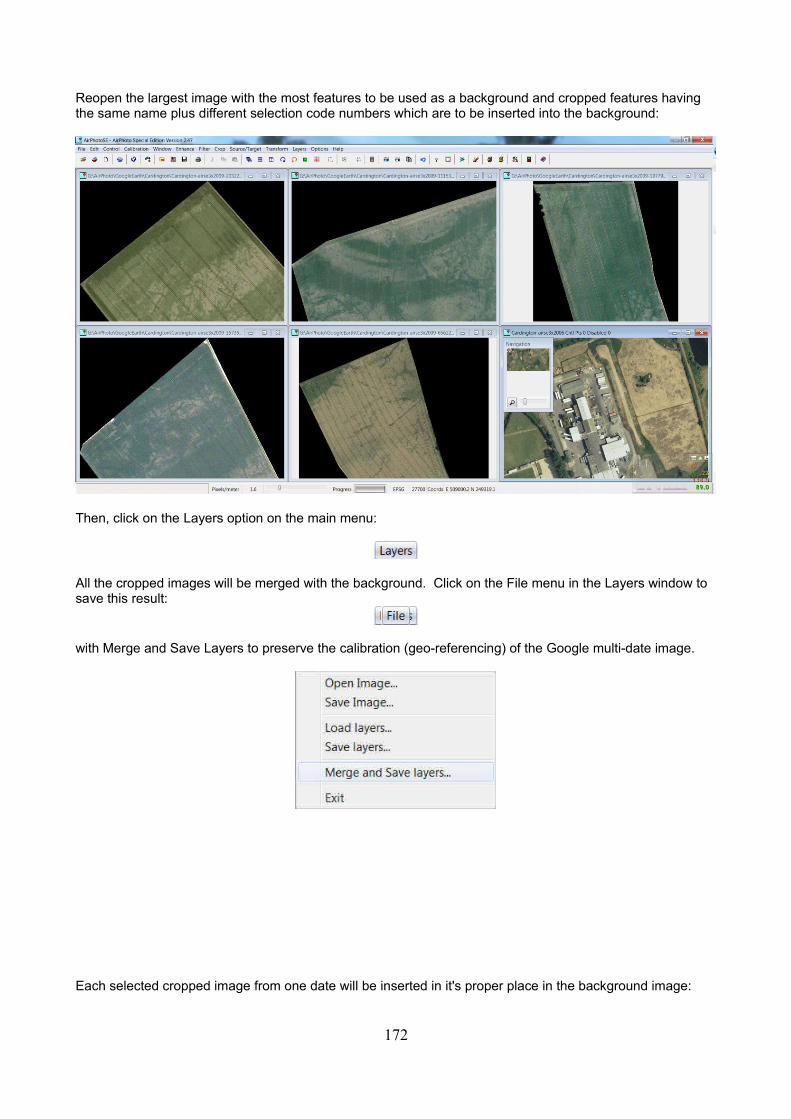
Reopen the largest image with the most features to be used as a background and cropped features having the same name plus different selection code numbers which are to be inserted into the background:

Then, click on the Layers option on the main menu:

All the cropped images will be merged with the background. Click on the File menu in the Layers window to save this result:

with Merge and Save Layers to preserve the calibration (geo-referencing) of the Google multi-date image.

Each selected cropped image from one date will be inserted in it's proper place in the background image:

172

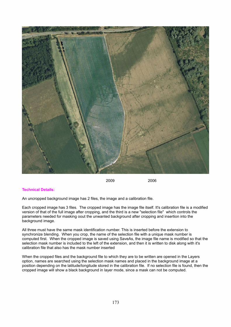
2009 2006

Technical Details:

An uncropped background image has 2 files, the image and a calibration file.

Each cropped image has 3 files. The cropped image has the image file itself. It's calibration file is a modified version of that of the full image after cropping, and the third is a new "selection file" which controls the parameters needed for masking oout the unwanted background after cropping and insertion into the background image.

All three must have the same mask identification number. This is inserted before the extension to synchronize blending. When you crop, the name of the selection file with a unique mask number is computed first. When the cropped image is saved using SaveAs, the image file name is modified so that the selection mask number is included to the left of the extension, and then it is written to disk along with it's calibration file that also has the mask number inserted

When the cropped files and the background file to which they are to be written are opened in the Layers option, names are searched using the selection mask names and placed in the background image at a position depending on the latitude/longitude stored in the calibration file. If no selection file is found, then thecropped image will show a black background in layer mode, since a mask can not be computed.

173

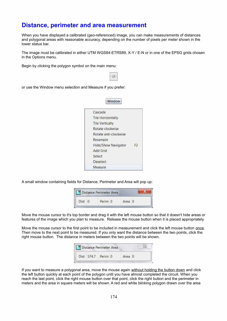
Distance, perimeter and area measurement

When you have displayed a calibrated (geo-referenced) image, you can make measurements of distances and polygonal areas with reasonable accuracy, depending on the number of pixels per meter shown in the lower status bar.

The image must be calibrated in either UTM WGS84-ETRS89, X-Y / E-N or in one of the EPSG grids chosenin the Options menu.

Begin by clicking the polygon symbol on the main menu:

or use the Window menu selection and Measure if you prefer:

A small window containing fields for Distance, Perimeter and Area will pop up:

Move the mouse cursor to it's top border and drag it with the left mouse button so that it doesn't hide areas orfeatures of the image which you plan to measure. Release the mouse button when it is placed appropriately.

Move the mouse cursor to the first point to be included in measurement and click the left mouse button once.Then move to the next point to be measured. If you only want the distance between the two points, click the right mouse button. The distance in meters between the two points will be shown.

If you want to measure a polygonal area, move the mouse again without holding the button down and click the left button quickly at each point of the polygon until you have almost completed the circuit. When you reach the last point, click the right mouse button over that point, click the right button and the perimeter in meters and the area in square meters will be shown. A red and white blinking polygon drawn over the area

174

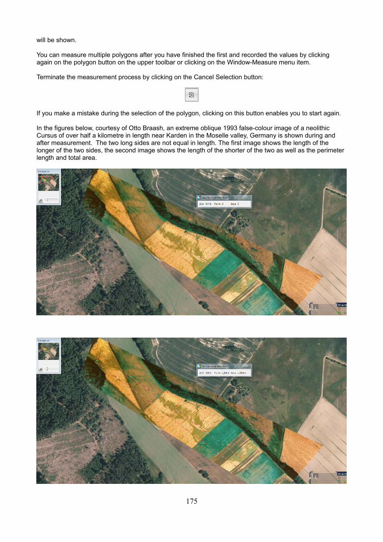
will be shown.

You can measure multiple polygons after you have finished the first and recorded the values by clicking again on the polygon button on the upper toolbar or clicking on the Window-Measure menu item.

Terminate the measurement process by clicking on the Cancel Selection button:

If you make a mistake during the selection of the polygon, clicking on this button enables you to start again.

In the figures below, courtesy of Otto Braash, an extreme oblique 1993 false-colour image of a neolithic Cursus of over half a kilometre in length near Karden in the Moselle valley, Germany is shown during and after measurement. The two long sides are not equal in length. The first image shows the length of the longer of the two sides, the second image shows the length of the shorter of the two as well as the perimeter length and total area.

175

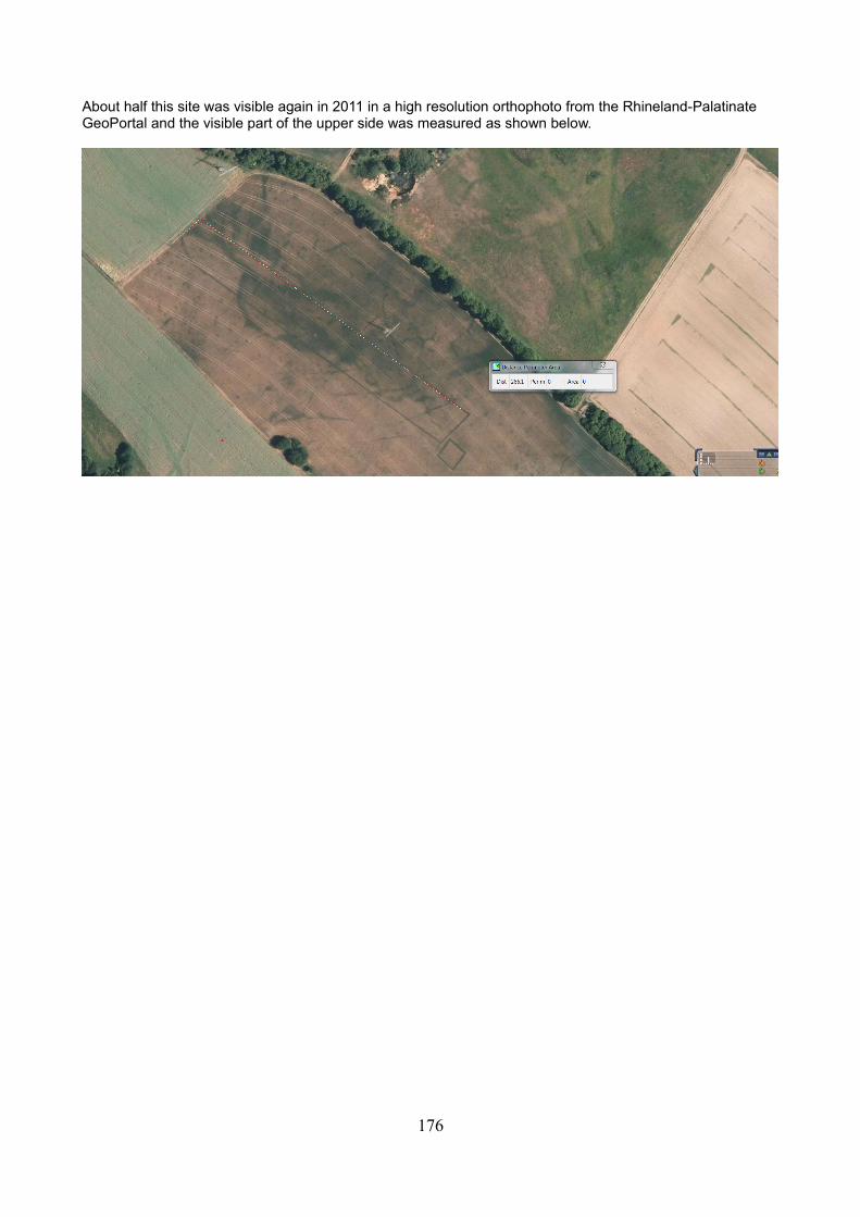
About half this site was visible again in 2011 in a high resolution orthophoto from the Rhineland-Palatinate GeoPortal and the visible part of the upper side was measured as shown below.

176

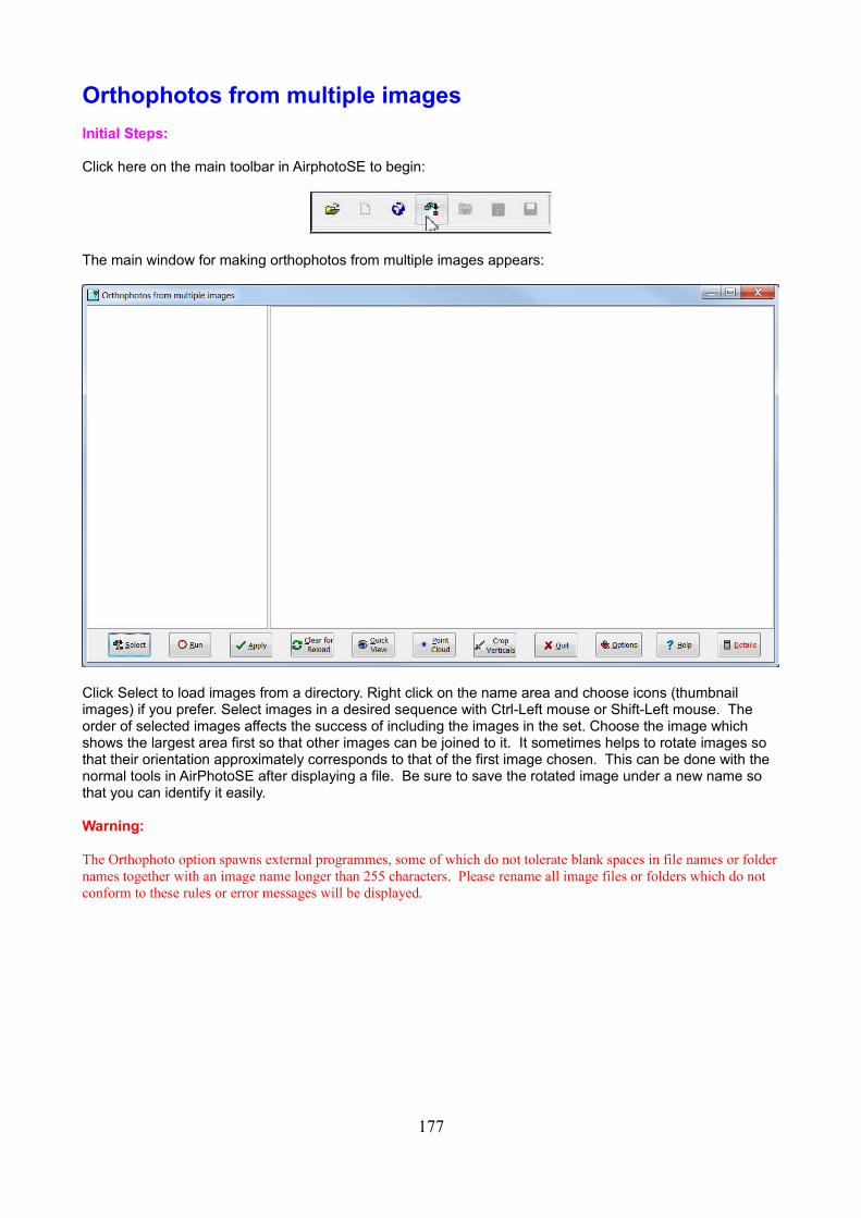
Orthophotos from multiple images

Initial Steps:

Click here on the main toolbar in AirphotoSE to begin:

The main window for making orthophotos from multiple images appears:

Click Select to load images from a directory. Right click on the name area and choose icons (thumbnail images) if you prefer. Select images in a desired sequence with Ctrl-Left mouse or Shift-Left mouse. The order of selected images affects the success of including the images in the set. Choose the image which shows the largest area first so that other images can be joined to it. It sometimes helps to rotate images so that their orientation approximately corresponds to that of the first image chosen. This can be done with the normal tools in AirPhotoSE after displaying a file. Be sure to save the rotated image under a new name so that you can identify it easily.

Warning:

The Orthophoto option spawns external programmes, some of which do not tolerate blank spaces in file names or foldernames together with an image name longer than 255 characters. Please rename all image files or folders which do not conform to these rules or error messages will be displayed.

177

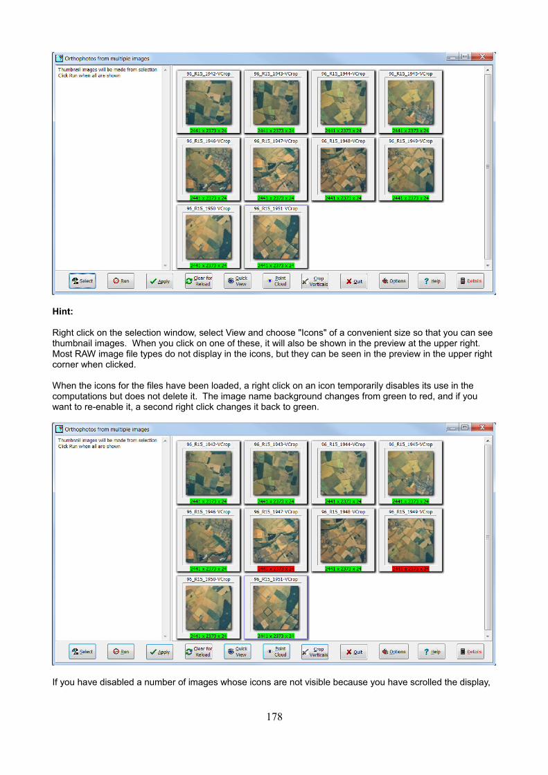
Hint:

Right click on the selection window, select View and choose "Icons" of a convenient size so that you can see thumbnail images. When you click on one of these, it will also be shown in the preview at the upper right. Most RAW image file types do not display in the icons, but they can be seen in the preview in the upper right corner when clicked.

When the icons for the files have been loaded, a right click on an icon temporarily disables its use in the computations but does not delete it. The image name background changes from green to red, and if you want to re-enable it, a second right click changes it back to green.

If you have disabled a number of images whose icons are not visible because you have scrolled the display,

178

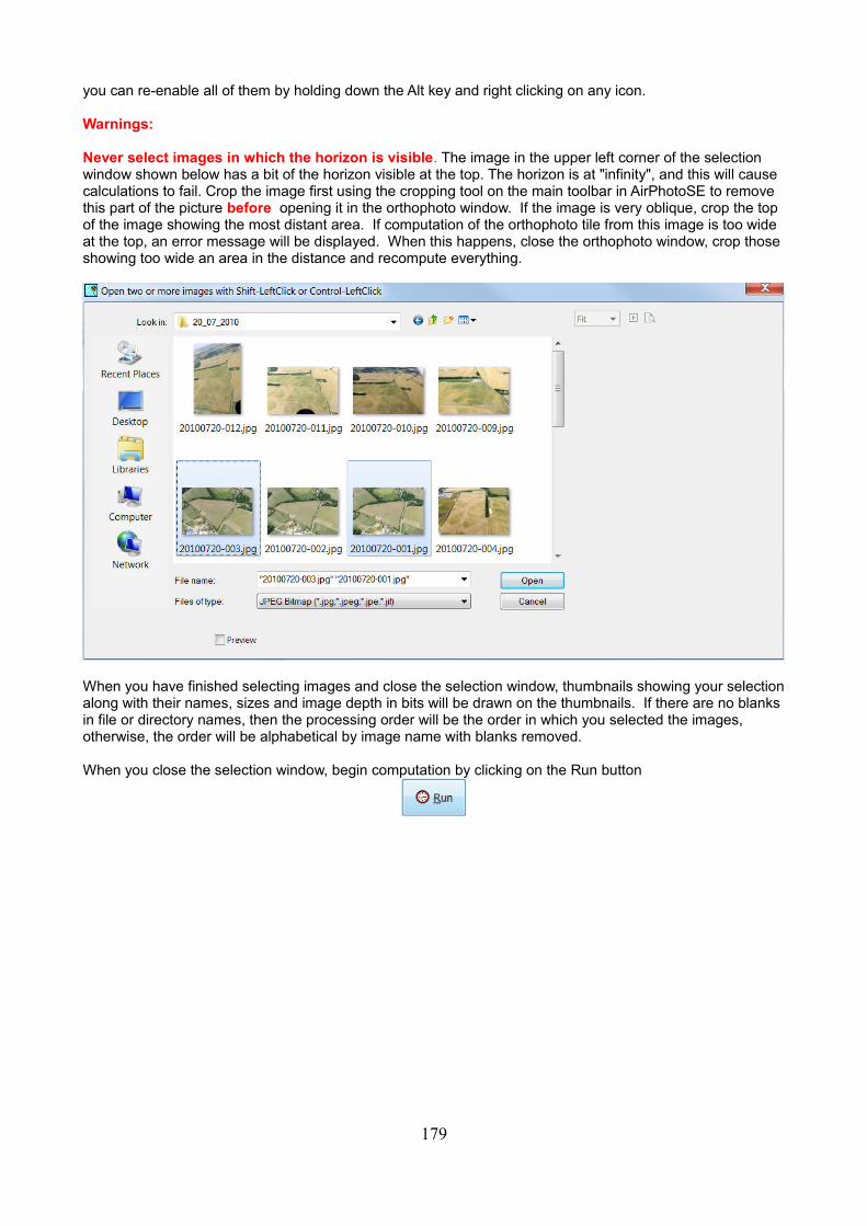
you can re-enable all of them by holding down the Alt key and right clicking on any icon.

Warnings:

Never select images in which the horizon is visible. The image in the upper left corner of the selection window shown below has a bit of the horizon visible at the top. The horizon is at "infinity", and this will cause calculations to fail. Crop the image first using the cropping tool on the main toolbar in AirPhotoSE to remove this part of the picture before opening it in the orthophoto window. If the image is very oblique, crop the top of the image showing the most distant area. If computation of the orthophoto tile from this image is too wide at the top, an error message will be displayed. When this happens, close the orthophoto window, crop those showing too wide an area in the distance and recompute everything.

When you have finished selecting images and close the selection window, thumbnails showing your selectionalong with their names, sizes and image depth in bits will be drawn on the thumbnails. If there are no blanks in file or directory names, then the processing order will be the order in which you selected the images, otherwise, the order will be alphabetical by image name with blanks removed.

When you close the selection window, begin computation by clicking on the Run button

179

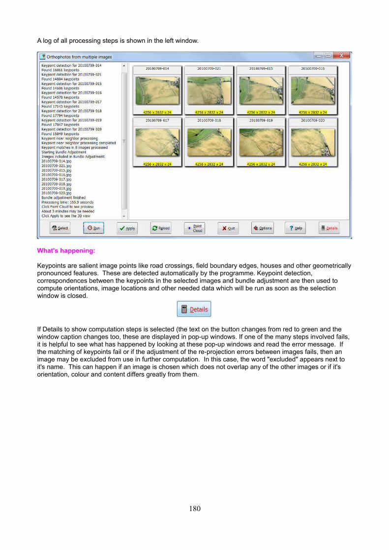
A log of all processing steps is shown in the left window.

What's happening:

Keypoints are salient image points like road crossings, field boundary edges, houses and other geometricallypronounced features. These are detected automatically by the programme. Keypoint detection, correspondences between the keypoints in the selected images and bundle adjustment are then used to compute orientations, image locations and other needed data which will be run as soon as the selection window is closed.

If Details to show computation steps is selected (the text on the button changes from red to green and the window caption changes too, these are displayed in pop-up windows. If one of the many steps involved fails, it is helpful to see what has happened by looking at these pop-up windows and read the error message. If the matching of keypoints fail or if the adjustment of the re-projection errors between images fails, then an image may be excluded from use in further computation. In this case, the word "excluded" appears next to it's name. This can happen if an image is chosen which does not overlap any of the other images or if it's orientation, colour and content differs greatly from them.

180

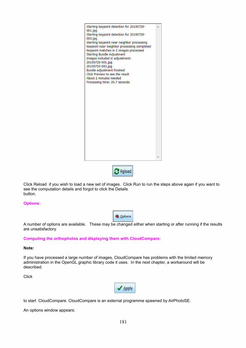
Click Reload if you wish to load a new set of images. Click Run to run the steps above again if you want to see the computation details and forgot to click the Details button.

Options:

A number of options are available. These may be changed either when starting or after running if the resultsare unsatisfactory.

Computing the orthophotos and displaying them with CloudCompare:

Note:

If you have processed a large number of images, CloudCompare has problems with the limited memory administration in the OpenGL graphic library code it uses. In the next chapter, a workaround will be described.

Click

to start CloudCompare. CloudCompare is an external programme spawned by AirPhotoSE.

An options window appears:

181

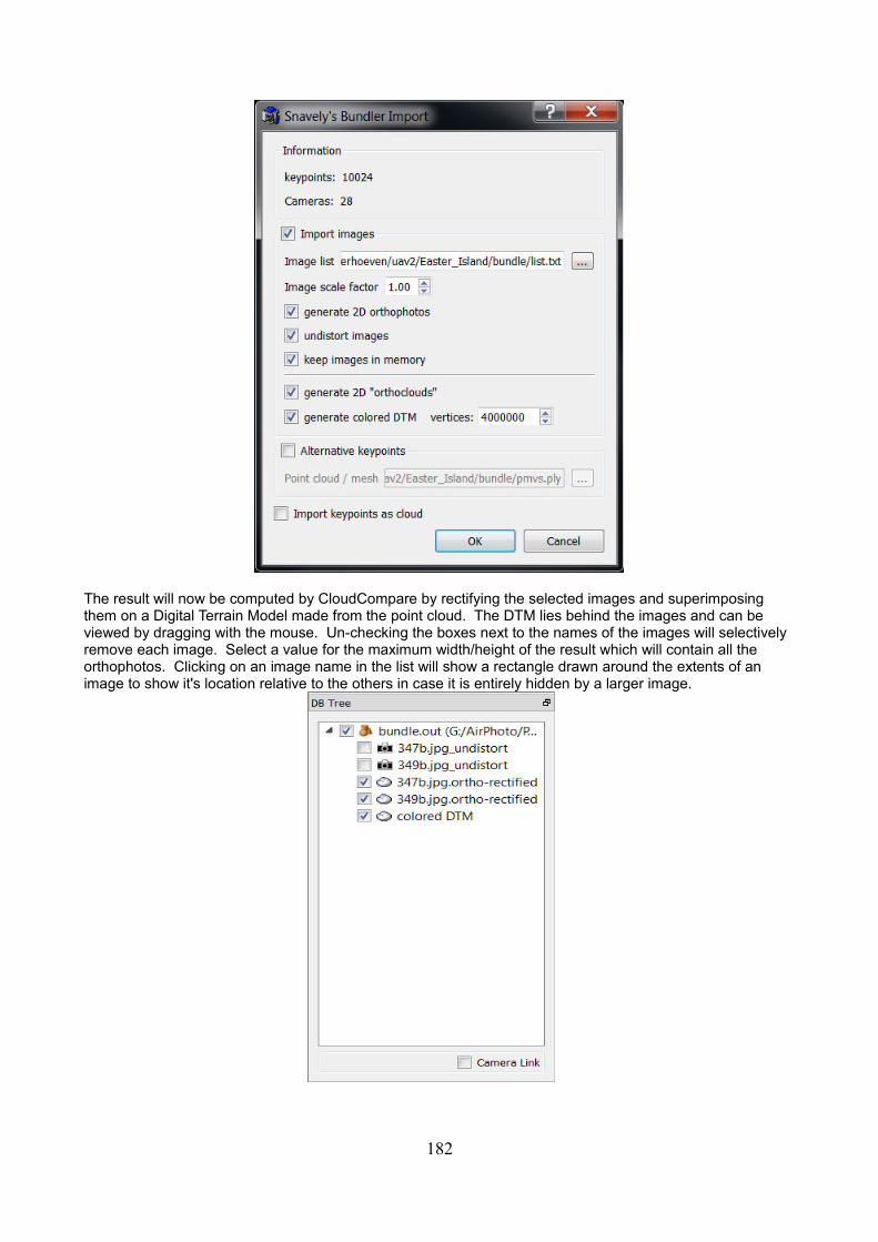
The result will now be computed by CloudCompare by rectifying the selected images and superimposing them on a Digital Terrain Model made from the point cloud. The DTM lies behind the images and can be viewed by dragging with the mouse. Un-checking the boxes next to the names of the images will selectively remove each image. Select a value for the maximum width/height of the result which will contain all the orthophotos. Clicking on an image name in the list will show a rectangle drawn around the extents of an image to show it's location relative to the others in case it is entirely hidden by a larger image.

182

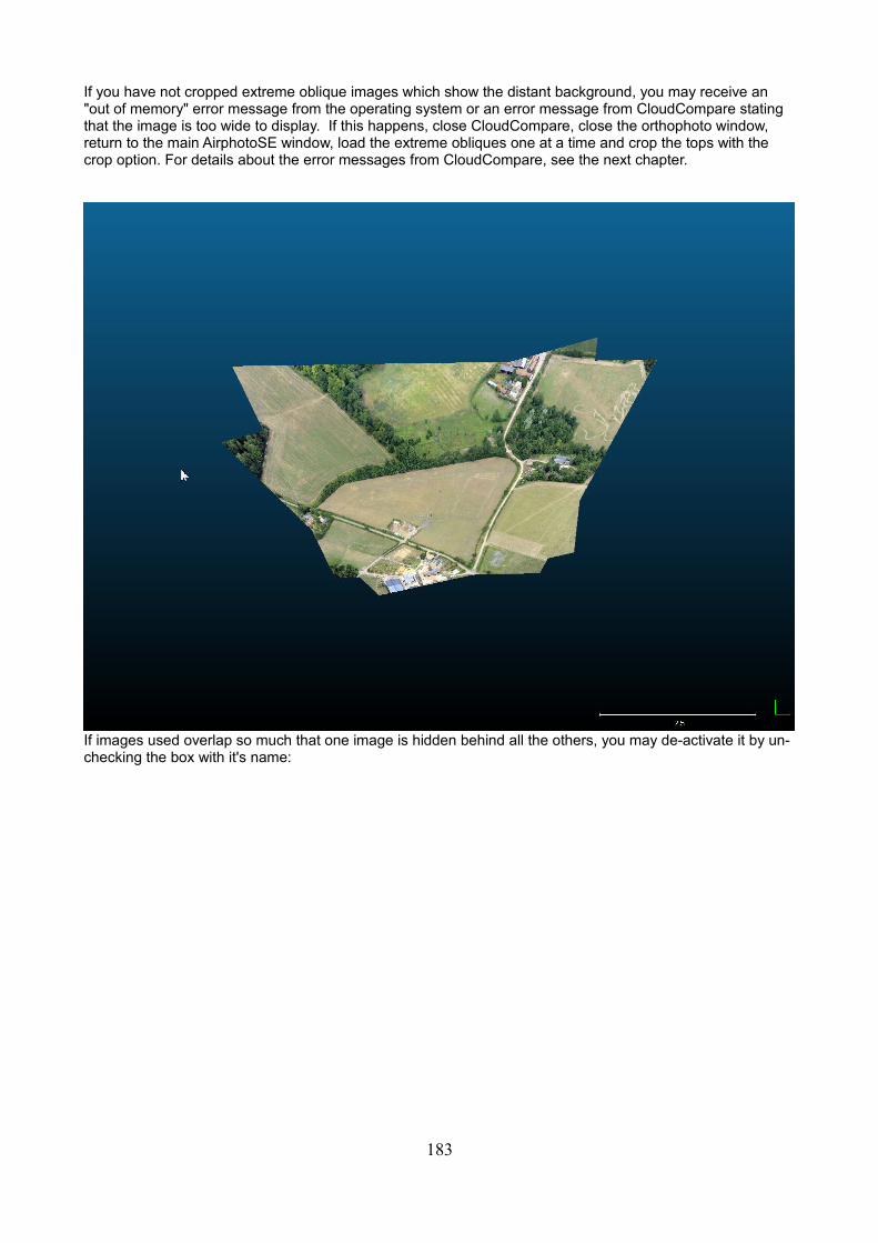
If you have not cropped extreme oblique images which show the distant background, you may receive an "out of memory" error message from the operating system or an error message from CloudCompare stating that the image is too wide to display. If this happens, close CloudCompare, close the orthophoto window, return to the main AirphotoSE window, load the extreme obliques one at a time and crop the tops with the crop option. For details about the error messages from CloudCompare, see the next chapter.

If images used overlap so much that one image is hidden behind all the others, you may de-activate it by un-checking the box with it's name:

183

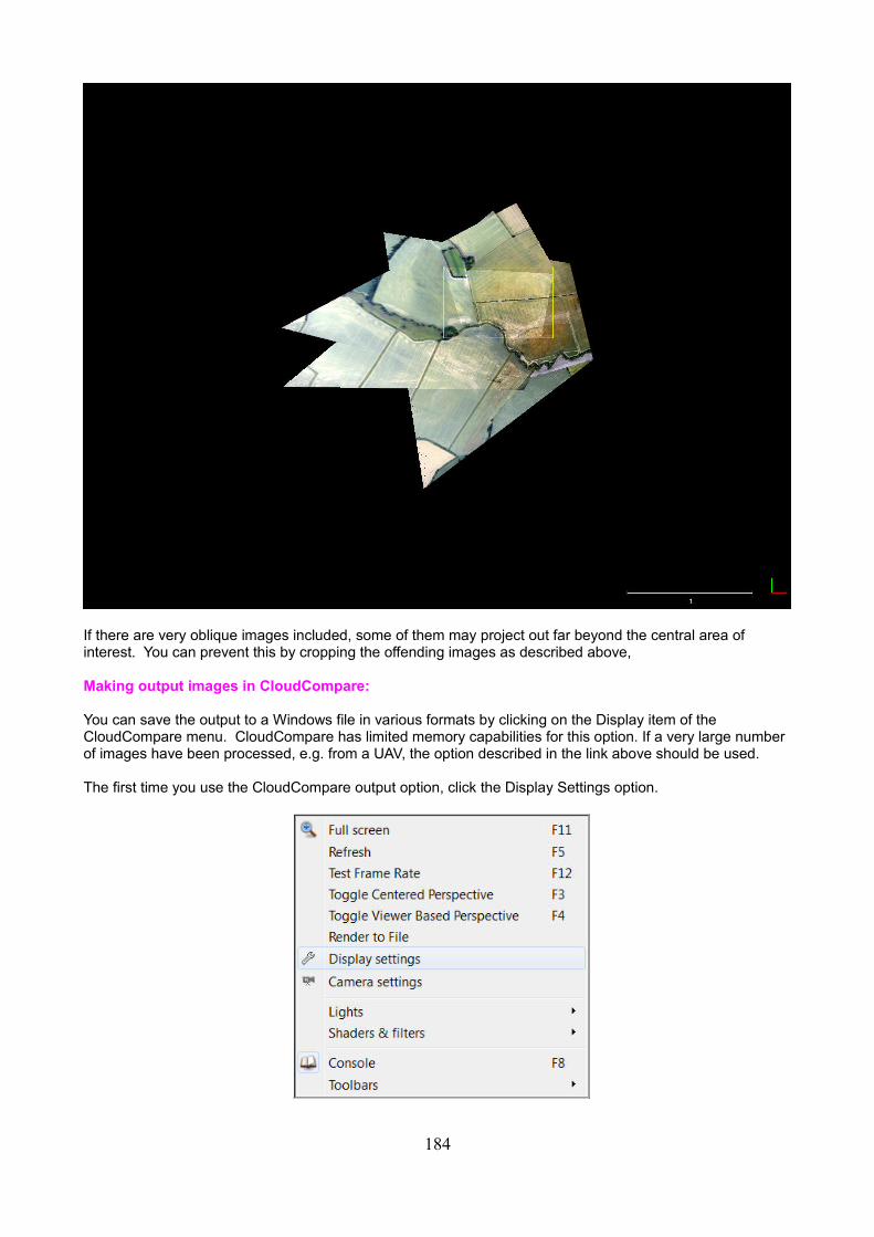
If there are very oblique images included, some of them may project out far beyond the central area of interest. You can prevent this by cropping the offending images as described above,

Making output images in CloudCompare:

You can save the output to a Windows file in various formats by clicking on the Display item of the CloudCompare menu. CloudCompare has limited memory capabilities for this option. If a very large number of images have been processed, e.g. from a UAV, the option described in the link above should be used.

The first time you use the CloudCompare output option, click the Display Settings option.

184

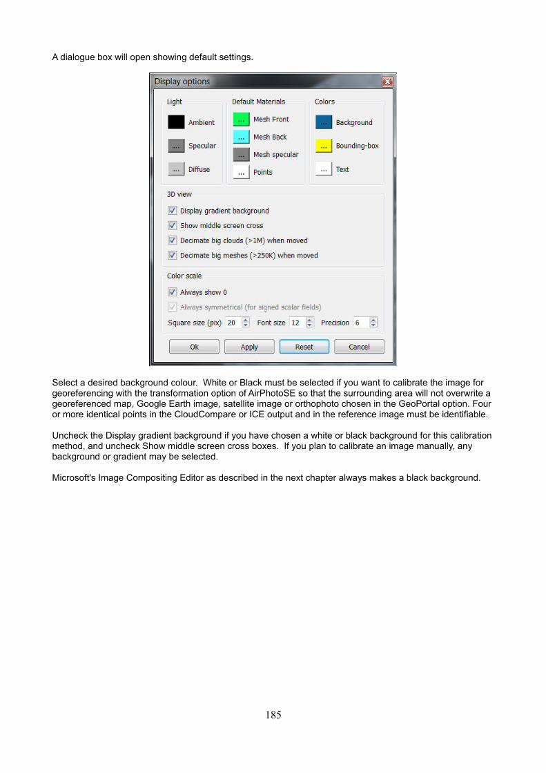
A dialogue box will open showing default settings.

Select a desired background colour. White or Black must be selected if you want to calibrate the image for georeferencing with the transformation option of AirPhotoSE so that the surrounding area will not overwrite a georeferenced map, Google Earth image, satellite image or orthophoto chosen in the GeoPortal option. Four or more identical points in the CloudCompare or ICE output and in the reference image must be identifiable.

Uncheck the Display gradient background if you have chosen a white or black background for this calibrationmethod, and uncheck Show middle screen cross boxes. If you plan to calibrate an image manually, any background or gradient may be selected.

Microsoft's Image Compositing Editor as described in the next chapter always makes a black background.

185

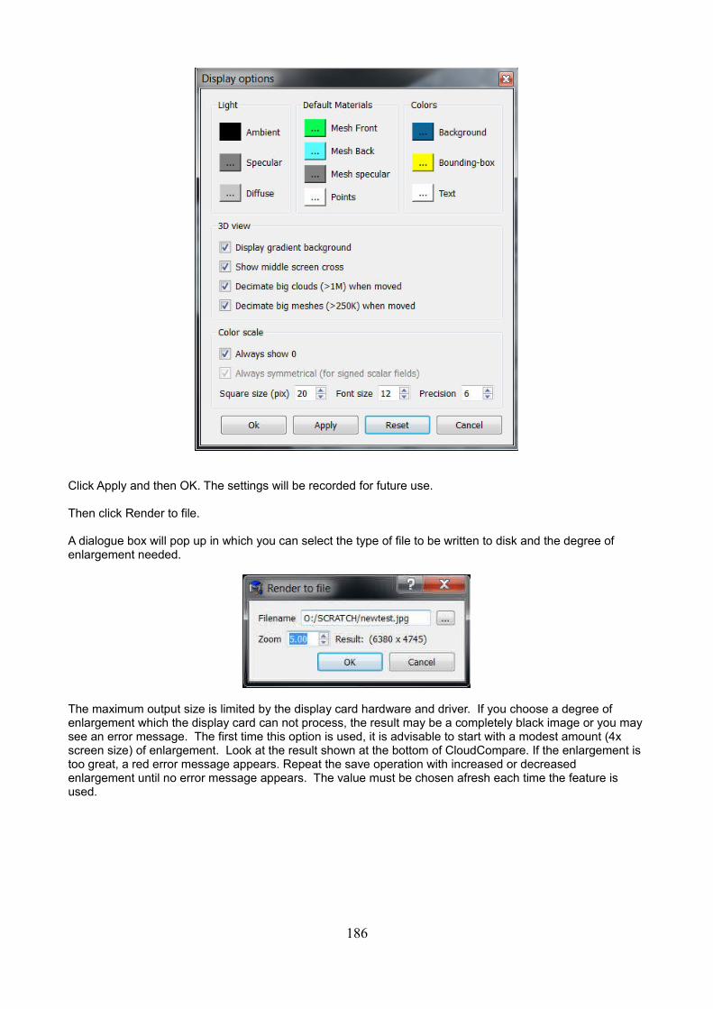
Click Apply and then OK. The settings will be recorded for future use.

Then click Render to file.

A dialogue box will pop up in which you can select the type of file to be written to disk and the degree of enlargement needed.

The maximum output size is limited by the display card hardware and driver. If you choose a degree of enlargement which the display card can not process, the result may be a completely black image or you maysee an error message. The first time this option is used, it is advisable to start with a modest amount (4x screen size) of enlargement. Look at the result shown at the bottom of CloudCompare. If the enlargement is too great, a red error message appears. Repeat the save operation with increased or decreased enlargement until no error message appears. The value must be chosen afresh each time the feature is used.

186

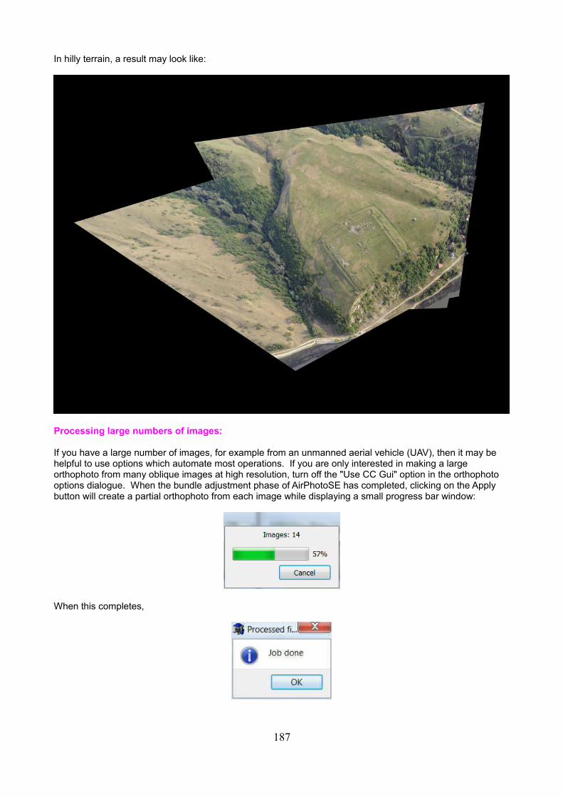
In hilly terrain, a result may look like:

Processing large numbers of images:

If you have a large number of images, for example from an unmanned aerial vehicle (UAV), then it may be helpful to use options which automate most operations. If you are only interested in making a large orthophoto from many oblique images at high resolution, turn off the "Use CC Gui" option in the orthophoto options dialogue. When the bundle adjustment phase of AirPhotoSE has completed, clicking on the Apply button will create a partial orthophoto from each image while displaying a small progress bar window:

When this completes,

187

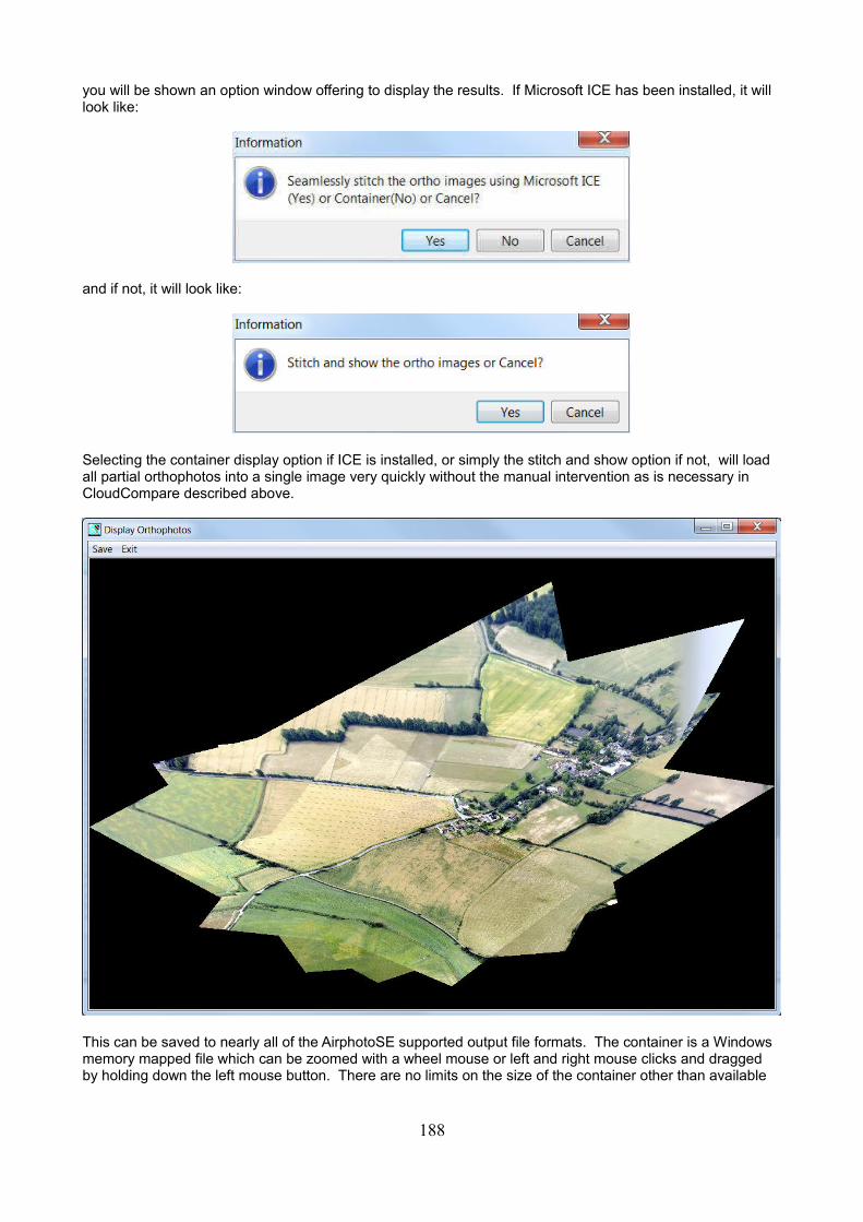
you will be shown an option window offering to display the results. If Microsoft ICE has been installed, it will look like:

and if not, it will look like:

Selecting the container display option if ICE is installed, or simply the stitch and show option if not, will load all partial orthophotos into a single image very quickly without the manual intervention as is necessary in CloudCompare described above.

This can be saved to nearly all of the AirphotoSE supported output file formats. The container is a Windows memory mapped file which can be zoomed with a wheel mouse or left and right mouse clicks and dragged by holding down the left mouse button. There are no limits on the size of the container other than available

188

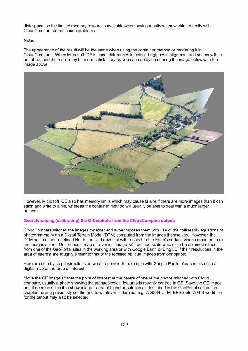
disk space, so the limited memory resources available when saving results when working directly with CloudCompare do not cause problems.

Note:

The appearance of the result will be the same when using the container method or rendering it in CloudCompare. When Microsoft ICE is used, differences in colour, brightness, alignment and seams will be equalized and the result may be more satisfactory as you can see by comparing the image below with the image above.

However, Microsoft ICE also has memory limits which may cause failure if there are more images than it can stitch and write to a file, whereas the container method will usually be able to deal with a much larger number.

Georeferencing (calibrating) the Orthophoto from the CloudCompare output:

CloudCompare stitches the images together and superimposes them with use of the collinearity equations of photogrammetry on a Digital Terrain Model (DTM) computed from the images themselves. However, the DTM has neither a defined North nor is it horizontal with respect to the Earth's surface when computed from the images alone. One needs a map or a vertical image with defined scale which can be obtained either from one of the GeoPortal sites in the working area or with Google Earth or Bing 3D if their resolutions in the area of interest are roughly similar to that of the rectified oblique images from orthophoto.

Here are step by step instructions on what to do next for example with Google Earth. You can also use a digital map of the area of interest.

Move the GE image so that the point of interest at the centre of one of the photos stitched with Cloud compare, usually a photo showing the archaeological features is roughly centred in GE. Save the GE image and if need be stitch it to show a larger area at higher resolution as described in the GeoPortal calibration chapter, having previously set the grid to whatever is desired, e.g. WGS84-UTM, EPSG etc. A GIS world file for the output may also be selected.

189

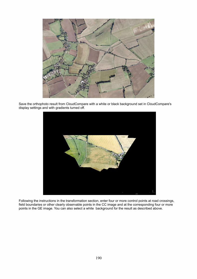
Save the orthophoto result from CloudCompare with a white or black background set in CloudCompare's display settings and with gradients turned off.

Following the instructions in the transformation section, enter four or more control points at road crossings, field boundaries or other clearly observable points in the CC image and at the corresponding four or more points in the GE image. You can also select a white background for the result as described above.

190

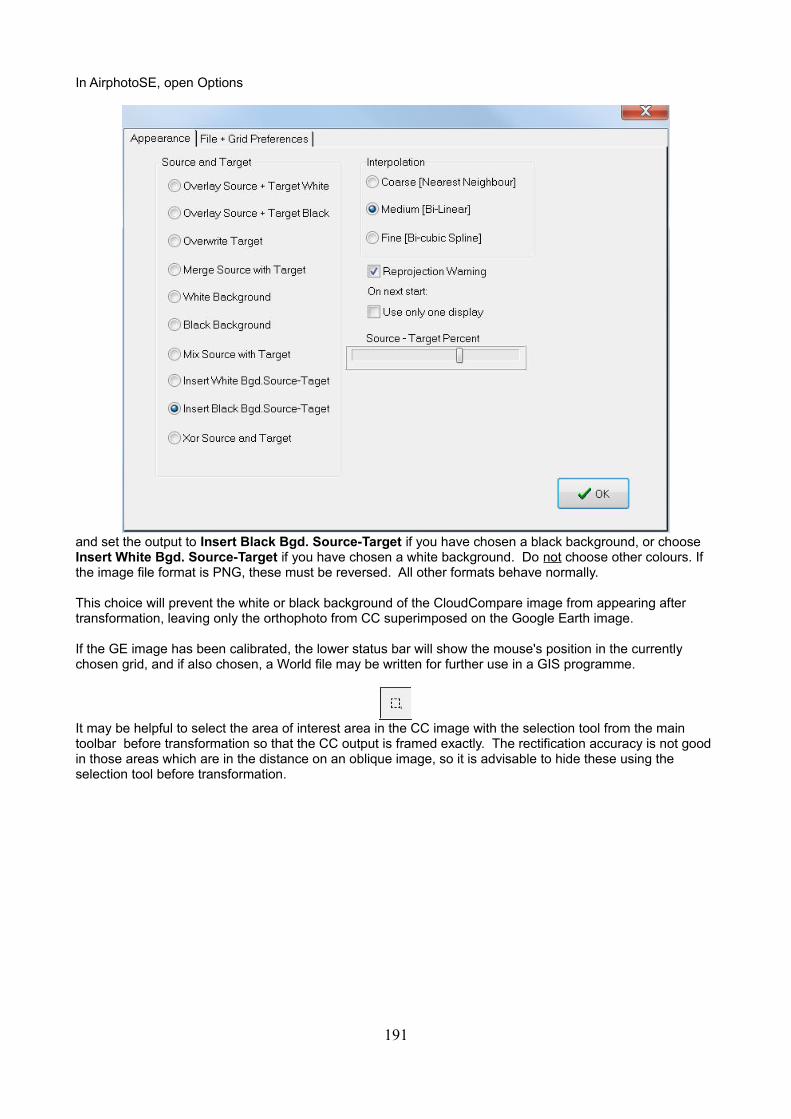
In AirphotoSE, open Options

and set the output to Insert Black Bgd. Source-Target if you have chosen a black background, or choose Insert White Bgd. Source-Target if you have chosen a white background. Do not choose other colours. If the image file format is PNG, these must be reversed. All other formats behave normally.

This choice will prevent the white or black background of the CloudCompare image from appearing after transformation, leaving only the orthophoto from CC superimposed on the Google Earth image.

If the GE image has been calibrated, the lower status bar will show the mouse's position in the currently chosen grid, and if also chosen, a World file may be written for further use in a GIS programme.

It may be helpful to select the area of interest area in the CC image with the selection tool from the main toolbar before transformation so that the CC output is framed exactly. The rectification accuracy is not good in those areas which are in the distance on an oblique image, so it is advisable to hide these using the selection tool before transformation.

191

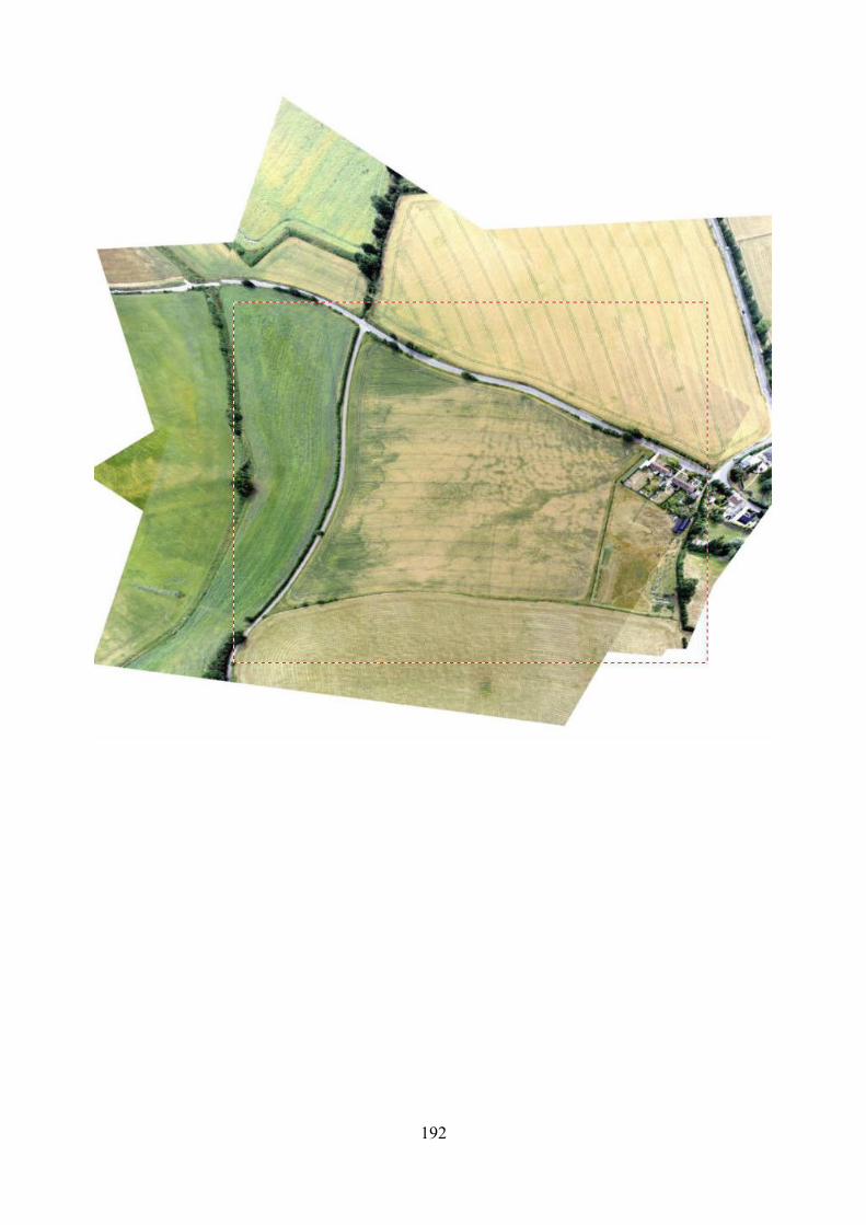
192

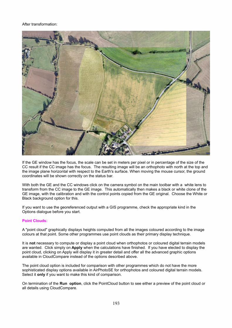
After transformation:

If the GE window has the focus, the scale can be set in meters per pixel or in percentage of the size of the CC result if the CC image has the focus. The resulting image will be an orthophoto with north at the top and the image plane horizontal with respect to the Earth's surface. When moving the mouse cursor, the ground coordinates will be shown correctly on the status bar.

With both the GE and the CC windows click on the camera symbol on the main toolbar with a white lens to transform from the CC image to the GE image. This automatically then makes a black or white clone of the GE image, with the calibration and with the control points copied from the GE original. Choose the White or Black background option for this.

If you want to use the georeferenced output with a GIS programme, check the appropriate kind in the Options dialogue before you start.

Point Clouds:

A "point cloud" graphically displays heights computed from all the images coloured according to the image colours at that point. Some other programmes use point clouds as their primary display technique.

It is not necessary to compute or display a point cloud when orthophotos or coloured digital terrain models are wanted. Click simply on Apply when the calculations have finished. If you have elected to display the point cloud, clicking on Apply will display it in greater detail and offer all the advanced graphic options available in CloudCompare instead of the options described above.

The point cloud option is included for comparison with other programmes which do not have the more sophisticated display options available in AirPhotoSE for orthophotos and coloured digital terrain models. Select it only if you want to make this kind of comparison.

On termination of the Run option, click the PointCloud button to see either a preview of the point cloud or all details using CloudCompare.

193

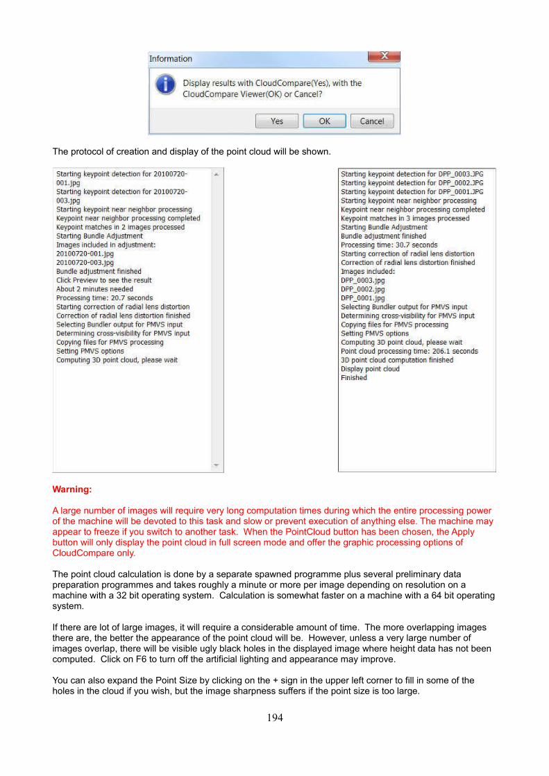
The protocol of creation and display of the point cloud will be shown.

Warning:

A large number of images will require very long computation times during which the entire processing power of the machine will be devoted to this task and slow or prevent execution of anything else. The machine may appear to freeze if you switch to another task. When the PointCloud button has been chosen, the Apply button will only display the point cloud in full screen mode and offer the graphic processing options of CloudCompare only.

The point cloud calculation is done by a separate spawned programme plus several preliminary data preparation programmes and takes roughly a minute or more per image depending on resolution on a machine with a 32 bit operating system. Calculation is somewhat faster on a machine with a 64 bit operatingsystem.

If there are lot of large images, it will require a considerable amount of time. The more overlapping images there are, the better the appearance of the point cloud will be. However, unless a very large number of images overlap, there will be visible ugly black holes in the displayed image where height data has not been computed. Click on F6 to turn off the artificial lighting and appearance may improve.

You can also expand the Point Size by clicking on the + sign in the upper left corner to fill in some of the holes in the cloud if you wish, but the image sharpness suffers if the point size is too large.

194

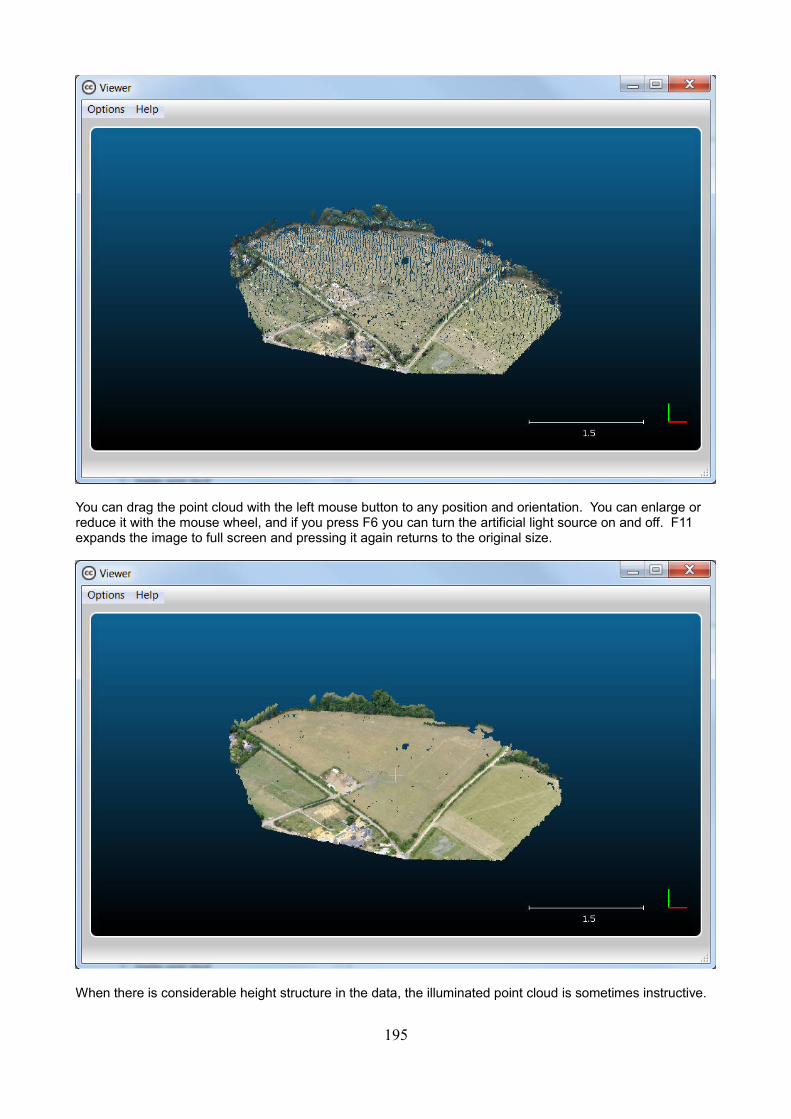
You can drag the point cloud with the left mouse button to any position and orientation. You can enlarge or reduce it with the mouse wheel, and if you press F6 you can turn the artificial light source on and off. F11 expands the image to full screen and pressing it again returns to the original size.

When there is considerable height structure in the data, the illuminated point cloud is sometimes instructive.

195

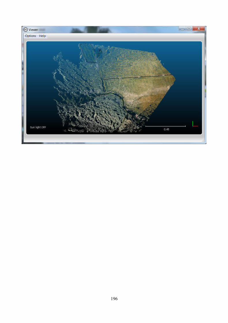
196

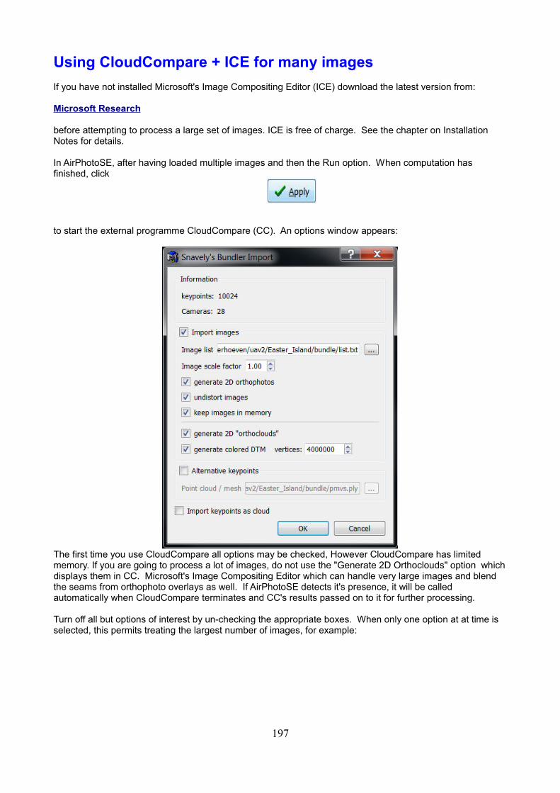
Using CloudCompare + ICE for many images

If you have not installed Microsoft's Image Compositing Editor (ICE) download the latest version from:

Microsoft Research

before attempting to process a large set of images. ICE is free of charge. See the chapter on Installation Notes for details.

In AirPhotoSE, after having loaded multiple images and then the Run option. When computation has finished, click

to start the external programme CloudCompare (CC). An options window appears:

The first time you use CloudCompare all options may be checked, However CloudCompare has limited memory. If you are going to process a lot of images, do not use the "Generate 2D Orthoclouds" option whichdisplays them in CC. Microsoft's Image Compositing Editor which can handle very large images and blend the seams from orthophoto overlays as well. If AirPhotoSE detects it's presence, it will be called automatically when CloudCompare terminates and CC's results passed on to it for further processing.

Turn off all but options of interest by un-checking the appropriate boxes. When only one option at at time is selected, this permits treating the largest number of images, for example:

197

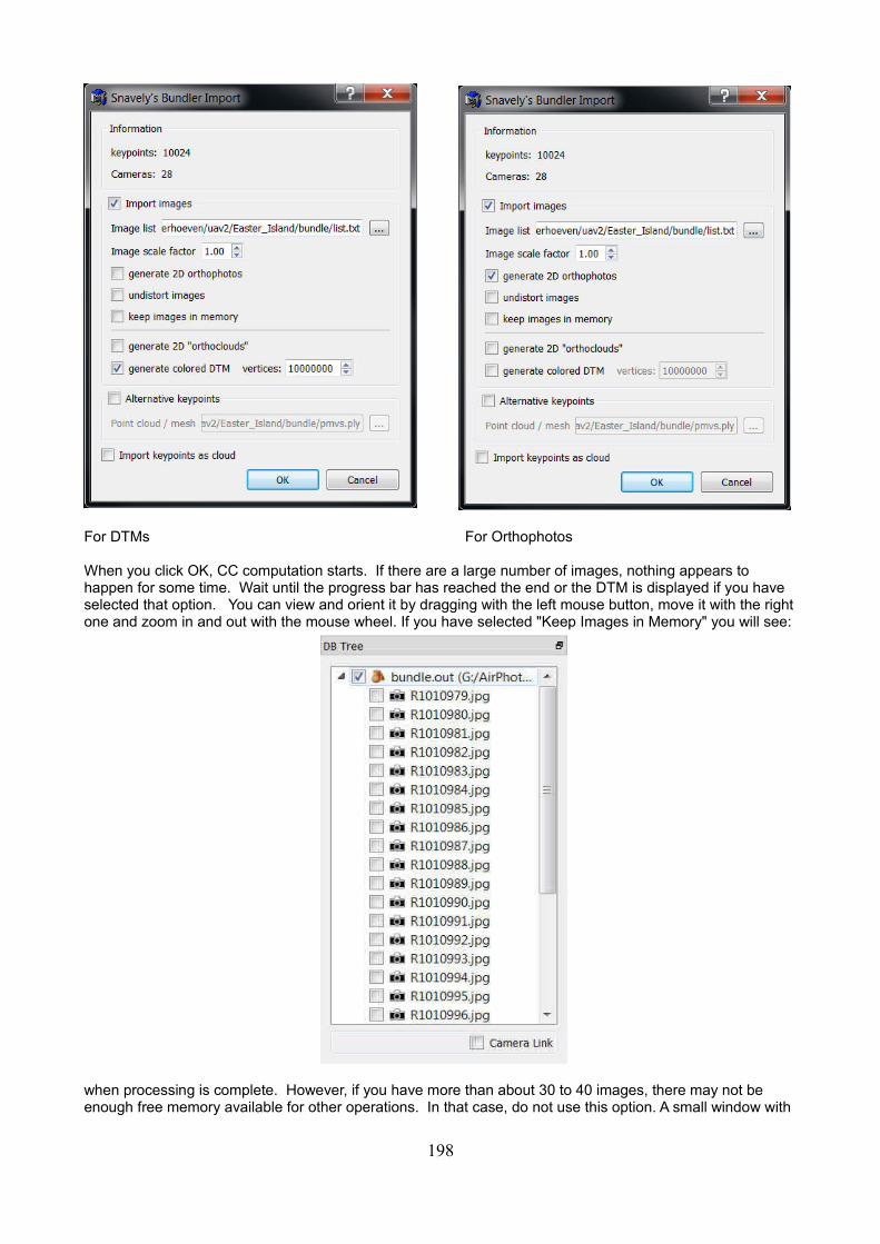
For DTMs For Orthophotos

When you click OK, CC computation starts. If there are a large number of images, nothing appears to happen for some time. Wait until the progress bar has reached the end or the DTM is displayed if you have selected that option. You can view and orient it by dragging with the left mouse button, move it with the rightone and zoom in and out with the mouse wheel. If you have selected "Keep Images in Memory" you will see:

when processing is complete. However, if you have more than about 30 to 40 images, there may not be enough free memory available for other operations. In that case, do not use this option. A small window with

198

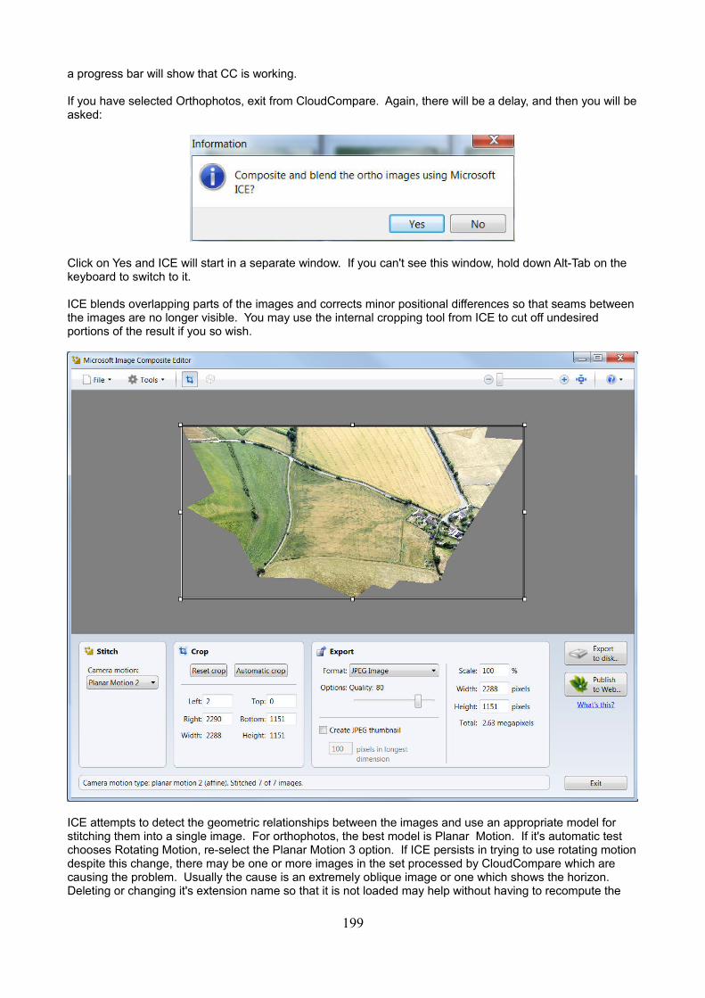
a progress bar will show that CC is working.

If you have selected Orthophotos, exit from CloudCompare. Again, there will be a delay, and then you will beasked:

Click on Yes and ICE will start in a separate window. If you can't see this window, hold down Alt-Tab on the keyboard to switch to it.

ICE blends overlapping parts of the images and corrects minor positional differences so that seams between the images are no longer visible. You may use the internal cropping tool from ICE to cut off undesired portions of the result if you so wish.

ICE attempts to detect the geometric relationships between the images and use an appropriate model for stitching them into a single image. For orthophotos, the best model is Planar Motion. If it's automatic test chooses Rotating Motion, re-select the Planar Motion 3 option. If ICE persists in trying to use rotating motiondespite this change, there may be one or more images in the set processed by CloudCompare which are causing the problem. Usually the cause is an extremely oblique image or one which shows the horizon. Deleting or changing it's extension name so that it is not loaded may help without having to recompute the

199

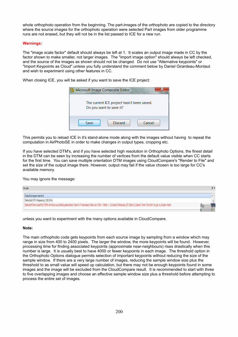
whole orthophoto operation from the beginning. The part-images of the orthophoto are copied to the directorywhere the source images for the orthophoto operation were selected Part images from older programme runs are not erased, but they will not be in the list passed to ICE for a new run.

Warnings:

The "image scale factor" default should always be left at 1. It scales an output image made in CC by the factor shown to make smaller, not larger images. The "import image option" should always be left checked, and the source of the images as shown should not be changed. Do not use "Alternative keypoints" or "Import Keypoints as Cloud".unless you fully understand the comment below by Daniel Girardeau-Montaut and wish to experiment using other features in CC.

When closing ICE, you will be asked if you want to save the ICE project:

This permits you to reload ICE in it's stand-alone mode along with the images without having to repeat the computation in AirPhotoSE in order to make changes in output types, cropping etc.

If you have selected DTM's, and if you have selected high resolution in Orthophoto Options, the finest detail in the DTM can be seen by increasing the number of vertices from the default value visible when CC starts for the first time. You can save multiple orientation DTM images using CloudCompare's "Render to File" and set the size of the output image there. However, output may fail if the value chosen is too large for CC's available memory.

You may ignore the message:

unless you want to experiment with the many options available in CloudCompare.

Note:

The main orthophoto code gets keypoints from each source image by sampling from a window which may range in size from 400 to 2400 pixels. The larger the window, the more keypoints will be found. However, processing time for finding associated keypoints (approximate near-neighbours) rises drastically when this number is large. It is usually best to have 4000 or fewer keypoints in each image. The threshold option in the Orthophoto Options dialogue permits selection of important keypoints without reducing the size of the sample window. If there are a very large number of images, reducing the sample window size plus the threshold to as small value will speed up calculation, but there may not be enough keypoints found in some images and the image will be excluded from the CloudCompare result. It is recommended to start with three to five overlapping images and choose an effective sample window size plus a threshold before attempting toprocess the entire set of images.

200

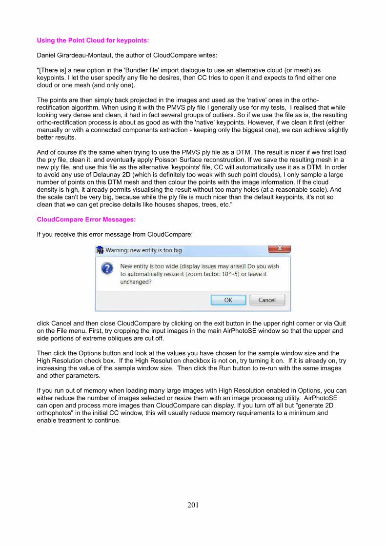
Using the Point Cloud for keypoints:

Daniel Girardeau-Montaut, the author of CloudCompare writes:

"[There is] a new option in the 'Bundler file' import dialogue to use an alternative cloud (or mesh) as keypoints. I let the user specify any file he desires, then CC tries to open it and expects to find either one cloud or one mesh (and only one).

The points are then simply back projected in the images and used as the 'native' ones in the ortho-rectification algorithm. When using it with the PMVS ply file I generally use for my tests, I realised that while looking very dense and clean, it had in fact several groups of outliers. So if we use the file as is, the resulting ortho-rectification process is about as good as with the 'native' keypoints. However, if we clean it first (either manually or with a connected components extraction - keeping only the biggest one), we can achieve slightlybetter results.

And of course it's the same when trying to use the PMVS ply file as a DTM. The result is nicer if we first load the ply file, clean it, and eventually apply Poisson Surface reconstruction. If we save the resulting mesh in a new ply file, and use this file as the alternative 'keypoints' file, CC will automatically use it as a DTM. In order to avoid any use of Delaunay 2D (which is definitely too weak with such point clouds), I only sample a large number of points on this DTM mesh and then colour the points with the image information. If the cloud density is high, it already permits visualising the result without too many holes (at a reasonable scale). And the scale can't be very big, because while the ply file is much nicer than the default keypoints, it's not so clean that we can get precise details like houses shapes, trees, etc."

CloudCompare Error Messages:

If you receive this error message from CloudCompare:

click Cancel and then close CloudCompare by clicking on the exit button in the upper right corner or via Quit on the File menu. First, try cropping the input images in the main AirPhotoSE window so that the upper and side portions of extreme obliques are cut off.

Then click the Options button and look at the values you have chosen for the sample window size and the High Resolution check box. If the High Resolution checkbox is not on, try turning it on. If it is already on, try increasing the value of the sample window size. Then click the Run button to re-run with the same images and other parameters.

If you run out of memory when loading many large images with High Resolution enabled in Options, you can either reduce the number of images selected or resize them with an image processing utility. AirPhotoSE can open and process more images than CloudCompare can display. If you turn off all but "generate 2D orthophotos" in the initial CC window, this will usually reduce memory requirements to a minimum and enable treatment to continue.

201

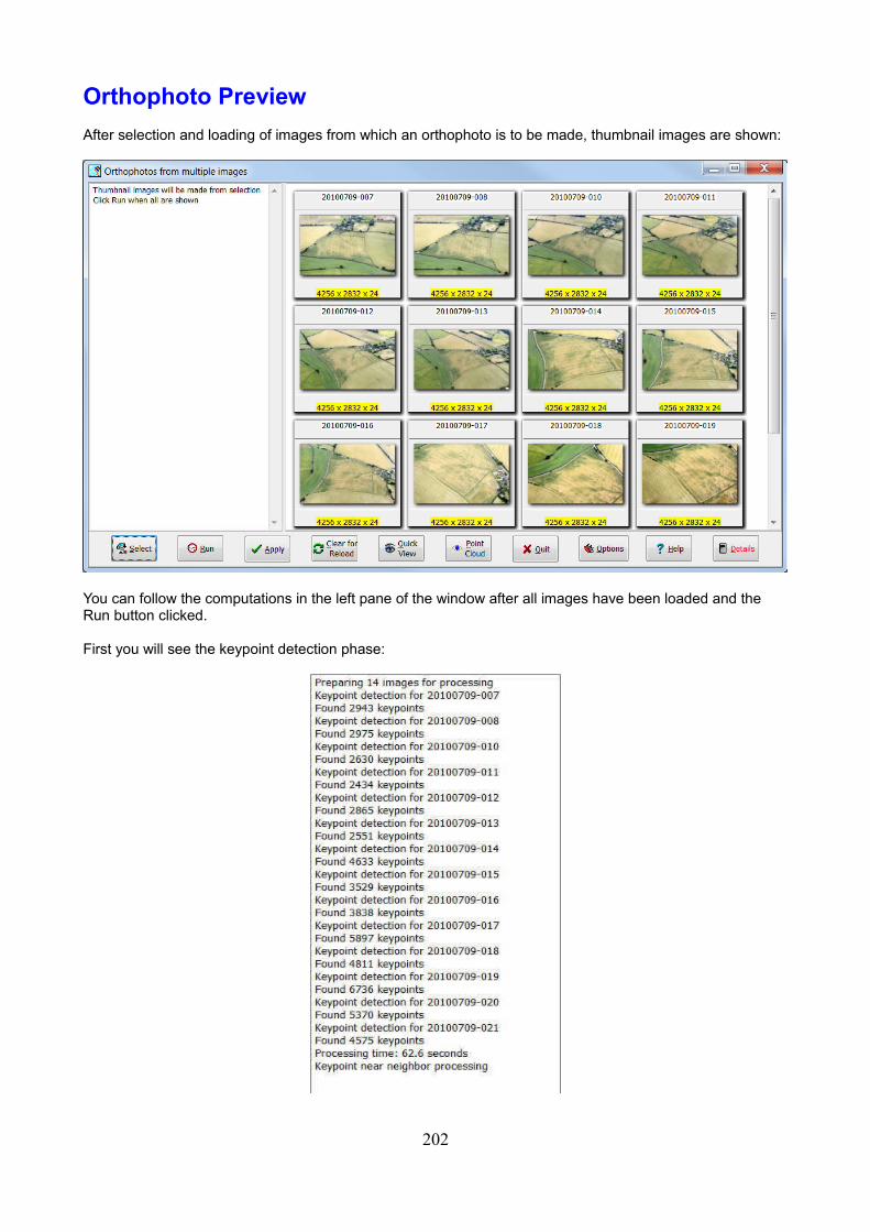
Orthophoto Preview

After selection and loading of images from which an orthophoto is to be made, thumbnail images are shown:

You can follow the computations in the left pane of the window after all images have been loaded and the Run button clicked.

First you will see the keypoint detection phase:

202

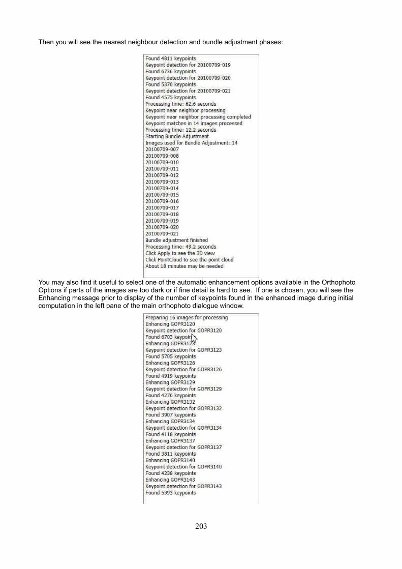
Then you will see the nearest neighbour detection and bundle adjustment phases:

You may also find it useful to select one of the automatic enhancement options available in the Orthophoto Options if parts of the images are too dark or if fine detail is hard to see. If one is chosen, you will see the Enhancing message prior to display of the number of keypoints found in the enhanced image during initial computation in the left pane of the main orthophoto dialogue window.

203

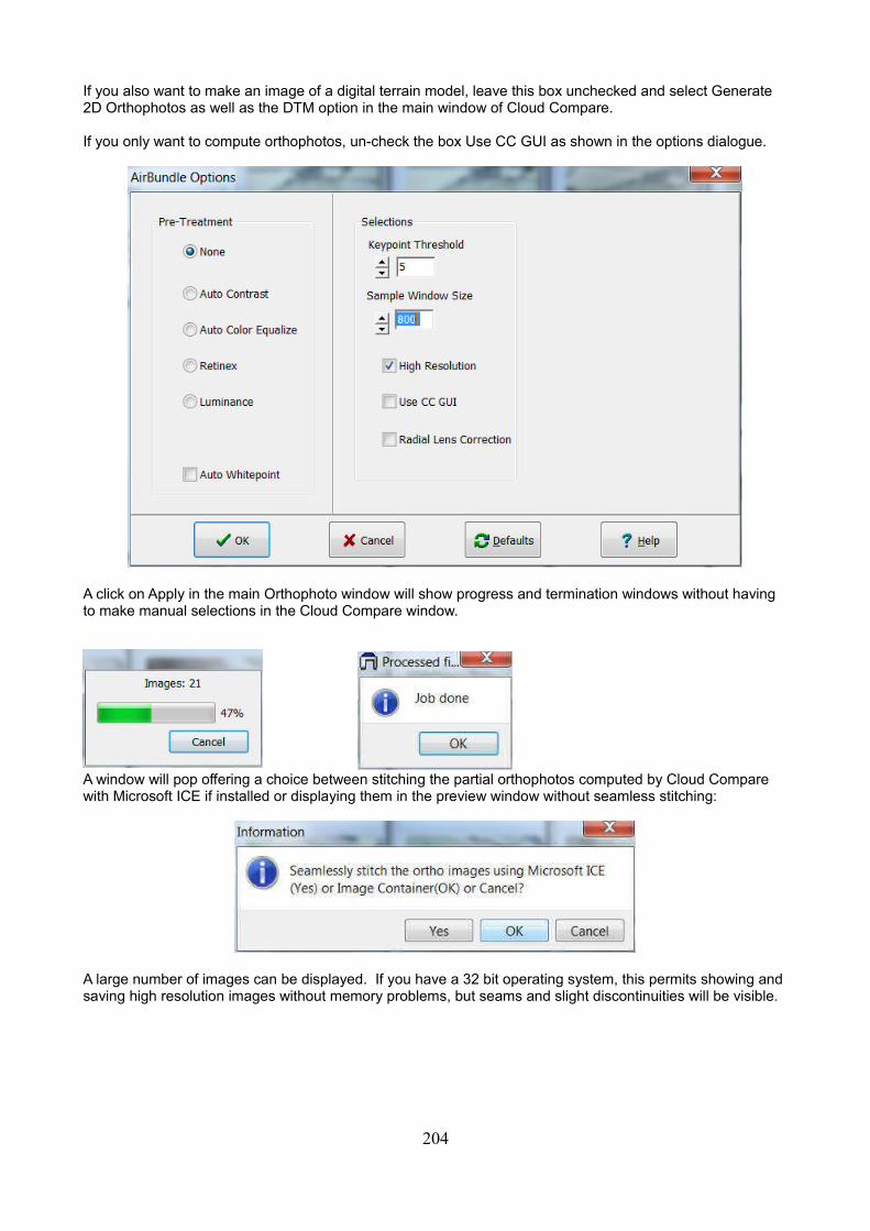
If you also want to make an image of a digital terrain model, leave this box unchecked and select Generate 2D Orthophotos as well as the DTM option in the main window of Cloud Compare.

If you only want to compute orthophotos, un-check the box Use CC GUI as shown in the options dialogue.

A click on Apply in the main Orthophoto window will show progress and termination windows without having to make manual selections in the Cloud Compare window.

A window will pop offering a choice between stitching the partial orthophotos computed by Cloud Compare with Microsoft ICE if installed or displaying them in the preview window without seamless stitching:

A large number of images can be displayed. If you have a 32 bit operating system, this permits showing and saving high resolution images without memory problems, but seams and slight discontinuities will be visible.

204

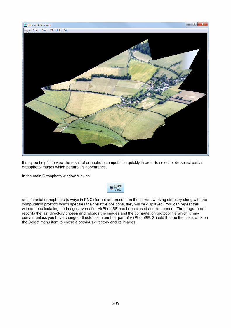
It may be helpful to view the result of orthophoto computation quickly in order to select or de-select partial orthophoto images which perturb it's appearance.

In the main Orthophoto window click on

and if partial orthophotos (always in PNG) format are present on the current working directory along with the computation protocol which specifies their relative positions, they will be displayed. You can repeat this without re-calculating the images even after AirPhotoSE has been closed and re-opened. The programme records the last directory chosen and reloads the images and the computation protocol file which it may contain unless you have changed directories in another part of AirPhotoSE. Should that be the case, click on the Select menu item to chose a previous directory and its images.

205

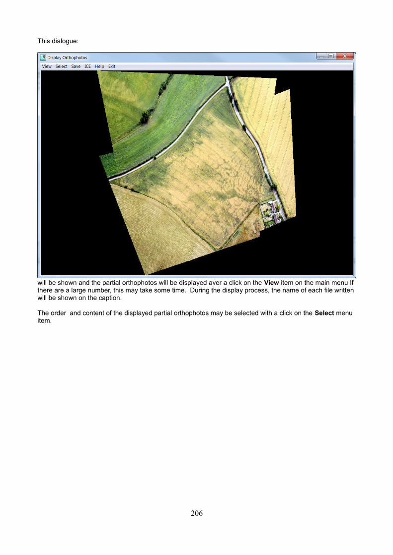
This dialogue:

will be shown and the partial orthophotos will be displayed aver a click on the View item on the main menu If there are a large number, this may take some time. During the display process, the name of each file writtenwill be shown on the caption.

The order and content of the displayed partial orthophotos may be selected with a click on the Select menu item.

206

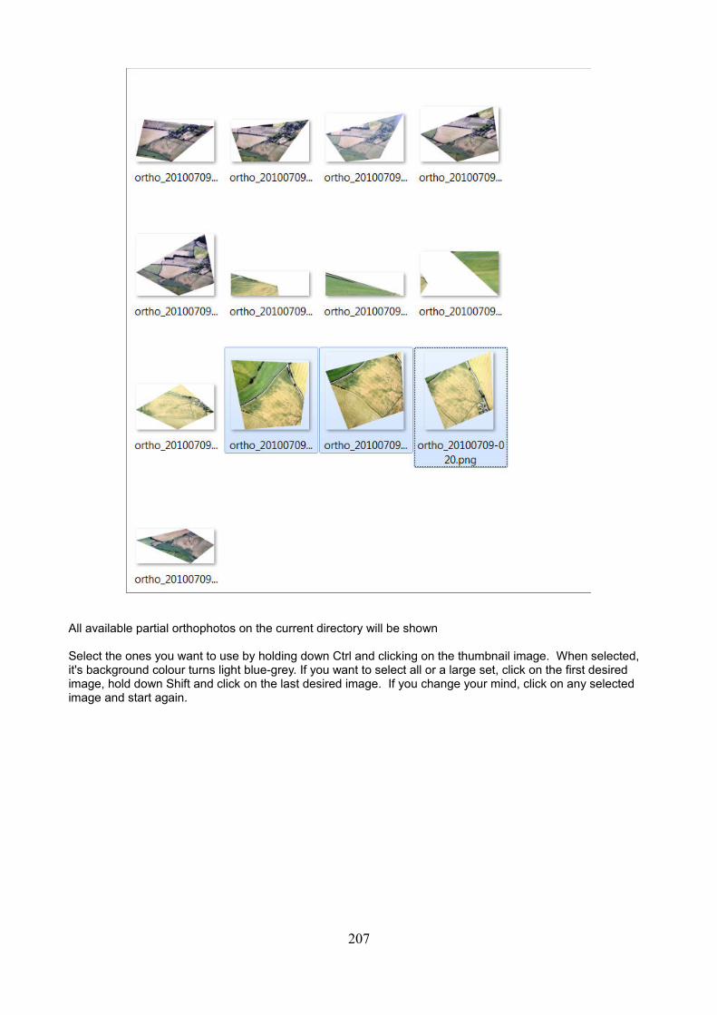
All available partial orthophotos on the current directory will be shown

Select the ones you want to use by holding down Ctrl and clicking on the thumbnail image. When selected, it's background colour turns light blue-grey. If you want to select all or a large set, click on the first desired image, hold down Shift and click on the last desired image. If you change your mind, click on any selected image and start again.

207

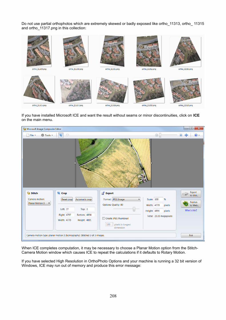
Do not use partial orthophotos which are extremely skewed or badly exposed like ortho_11313, ortho_ 11315and ortho_11317.png in this collection:

If you have installed Microsoft ICE and want the result without seams or minor discontinuities, click on ICE on the main menu.

When ICE completes computation, it may be necessary to choose a Planar Motion option from the Stitch-Camera Motion window which causes ICE to repeat the calculations if it defaults to Rotary Motion.

If you have selected High Resolution in OrthoPhoto Options and your machine is running a 32 bit version of Windows, ICE may run out of memory and produce this error message:

208

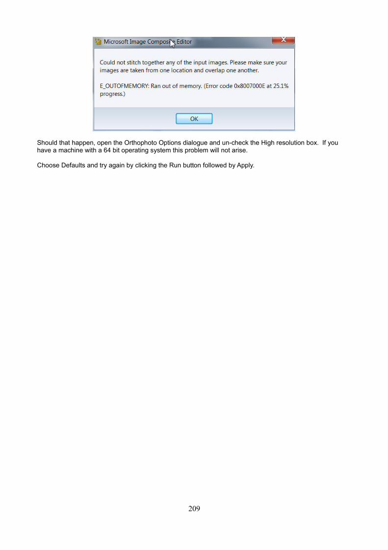
Should that happen, open the Orthophoto Options dialogue and un-check the High resolution box. If you have a machine with a 64 bit operating system this problem will not arise.

Choose Defaults and try again by clicking the Run button followed by Apply.

209

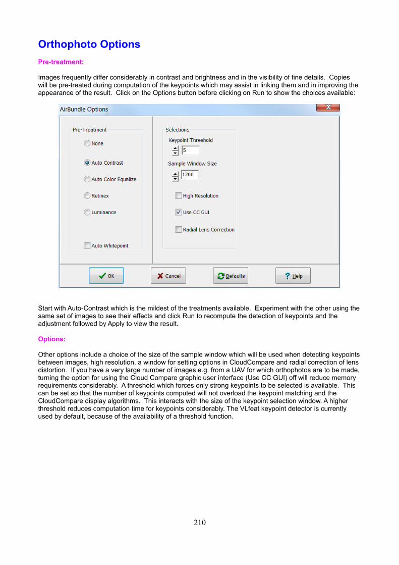
Orthophoto Options

Pre-treatment:

Images frequently differ considerably in contrast and brightness and in the visibility of fine details. Copies will be pre-treated during computation of the keypoints which may assist in linking them and in improving the appearance of the result. Click on the Options button before clicking on Run to show the choices available:

Start with Auto-Contrast which is the mildest of the treatments available. Experiment with the other using thesame set of images to see their effects and click Run to recompute the detection of keypoints and the adjustment followed by Apply to view the result.

Options:

Other options include a choice of the size of the sample window which will be used when detecting keypointsbetween images, high resolution, a window for setting options in CloudCompare and radial correction of lens distortion. If you have a very large number of images e.g. from a UAV for which orthophotos are to be made,turning the option for using the Cloud Compare graphic user interface (Use CC GUI) off will reduce memory requirements considerably. A threshold which forces only strong keypoints to be selected is available. This can be set so that the number of keypoints computed will not overload the keypoint matching and the CloudCompare display algorithms. This interacts with the size of the keypoint selection window. A higher threshold reduces computation time for keypoints considerably. The VLfeat keypoint detector is currently used by default, because of the availability of a threshold function.

210

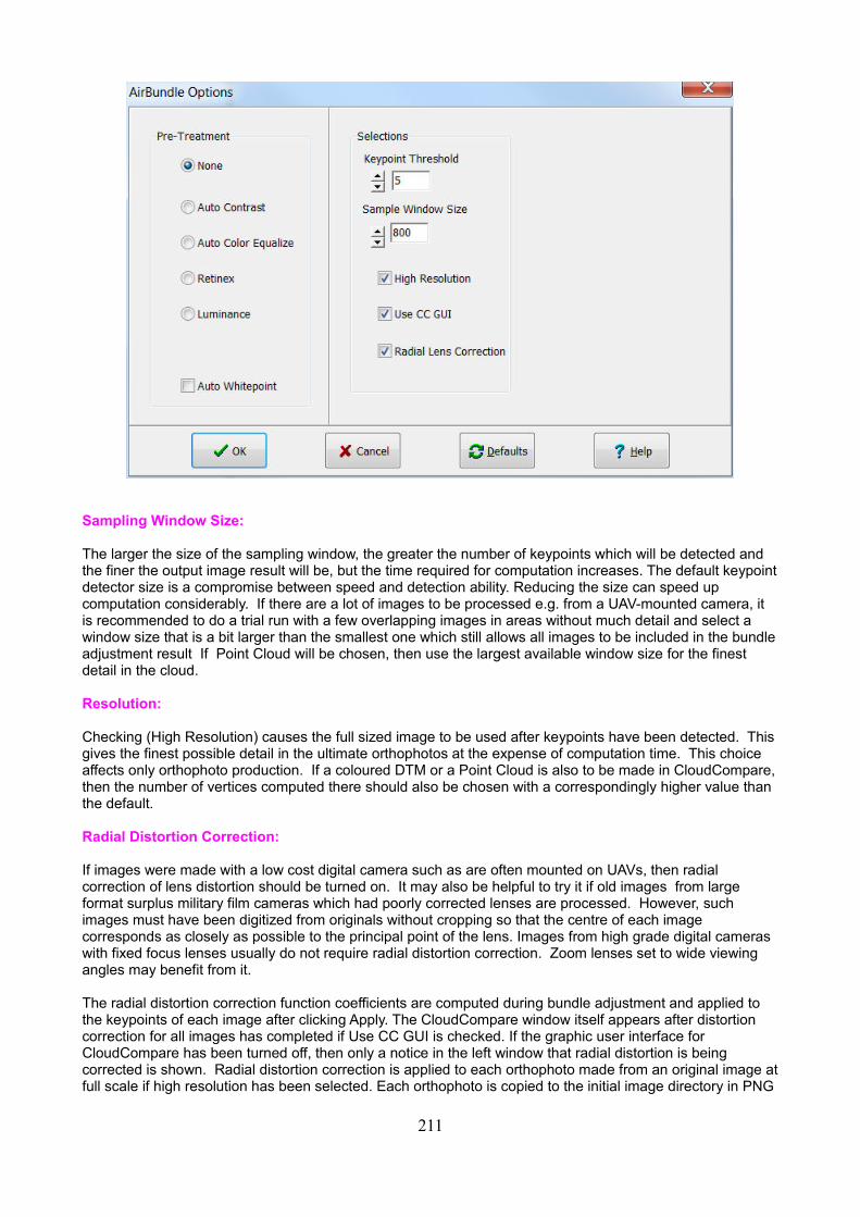
Sampling Window Size:

The larger the size of the sampling window, the greater the number of keypoints which will be detected and the finer the output image result will be, but the time required for computation increases. The default keypointdetector size is a compromise between speed and detection ability. Reducing the size can speed up computation considerably. If there are a lot of images to be processed e.g. from a UAV-mounted camera, it is recommended to do a trial run with a few overlapping images in areas without much detail and select a window size that is a bit larger than the smallest one which still allows all images to be included in the bundleadjustment result If Point Cloud will be chosen, then use the largest available window size for the finest detail in the cloud.

Resolution:

Checking (High Resolution) causes the full sized image to be used after keypoints have been detected. Thisgives the finest possible detail in the ultimate orthophotos at the expense of computation time. This choice affects only orthophoto production. If a coloured DTM or a Point Cloud is also to be made in CloudCompare,then the number of vertices computed there should also be chosen with a correspondingly higher value than the default.

Radial Distortion Correction:

If images were made with a low cost digital camera such as are often mounted on UAVs, then radial correction of lens distortion should be turned on. It may also be helpful to try it if old images from large format surplus military film cameras which had poorly corrected lenses are processed. However, such images must have been digitized from originals without cropping so that the centre of each image corresponds as closely as possible to the principal point of the lens. Images from high grade digital cameras with fixed focus lenses usually do not require radial distortion correction. Zoom lenses set to wide viewing angles may benefit from it.

The radial distortion correction function coefficients are computed during bundle adjustment and applied to the keypoints of each image after clicking Apply. The CloudCompare window itself appears after distortion correction for all images has completed if Use CC GUI is checked. If the graphic user interface for CloudCompare has been turned off, then only a notice in the left window that radial distortion is being corrected is shown. Radial distortion correction is applied to each orthophoto made from an original image atfull scale if high resolution has been selected. Each orthophoto is copied to the initial image directory in PNG

211

format. They can be individually calibrated and overlaid on maps, satellite images or true orthophotos from mapping agencies with greater accuracy in hilly terrain than that which is available without radial correction. Although only two images are required for computation of the radial distortion coefficients, more than two canimprove the accuracy of their computation somewhat.

Warning:

If radial distortion correction software like PTLens, RadCor or DXO has been used, do not turn on the correction, since this may introduce errors..

Note:

All chosen options are recorded when the programme is closed and their values written to the user's data in the Windows Registry. When the programme is restarted, these values are the defaults for the next computation if the same user is working with the programme. If you choose different data compared with thelast time the programme ran, it may be necessary to change the options.

212

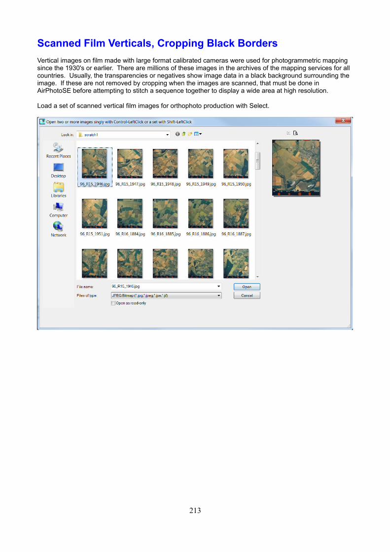
Scanned Film Verticals, Cropping Black Borders

Vertical images on film made with large format calibrated cameras were used for photogrammetric mapping since the 1930's or earlier. There are millions of these images in the archives of the mapping services for all countries. Usually, the transparencies or negatives show image data in a black background surrounding the image. If these are not removed by cropping when the images are scanned, that must be done in AirPhotoSE before attempting to stitch a sequence together to display a wide area at high resolution.

Load a set of scanned vertical film images for orthophoto production with Select.

213

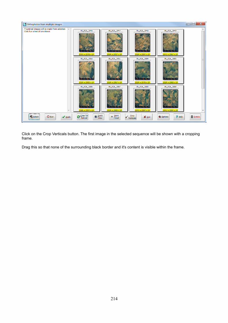
Click on the Crop Verticals button. The first image in the selected sequence will be shown with a cropping frame.

Drag this so that none of the surrounding black border and it's content is visible within the frame.

214

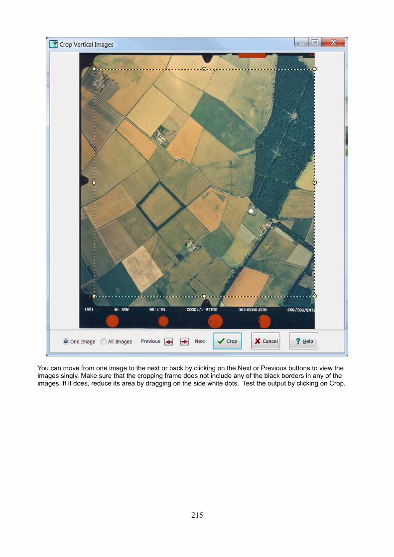
You can move from one image to the next or back by clicking on the Next or Previous buttons to view the images singly. Make sure that the cropping frame does not include any of the black borders in any of the images. If it does, reduce its area by dragging on the side white dots. Test the output by clicking on Crop.

215

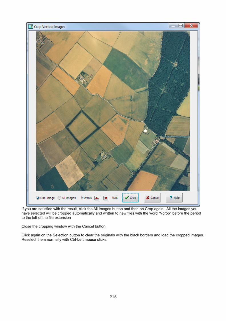
If you are satisfied with the result, click the All Images button and then on Crop again. All the images you have selected will be cropped automatically and written to new files with the word "Vcrop" before the period to the left of the file extension

Close the cropping window with the Cancel button.

Click again on the Selection button to clear the originals with the black borders and load the cropped images.Reselect them normally with Ctrl-Left mouse clicks.

216

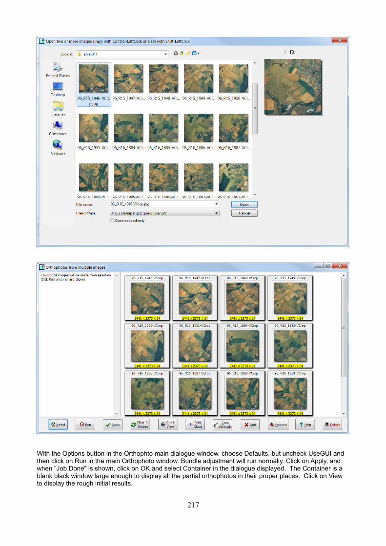
With the Options button in the Orthophto main dialogue window, choose Defaults, but uncheck UseGUI and then click on Run in the main Orthophoto window. Bundle adjustment will run normally. Click on Apply, and when "Job Done" is shown, click on OK and select Container in the dialogue displayed. The Container is a blank black window large enough to display all the partial orthophotos in their proper places. Click on View to display the rough initial results.

217

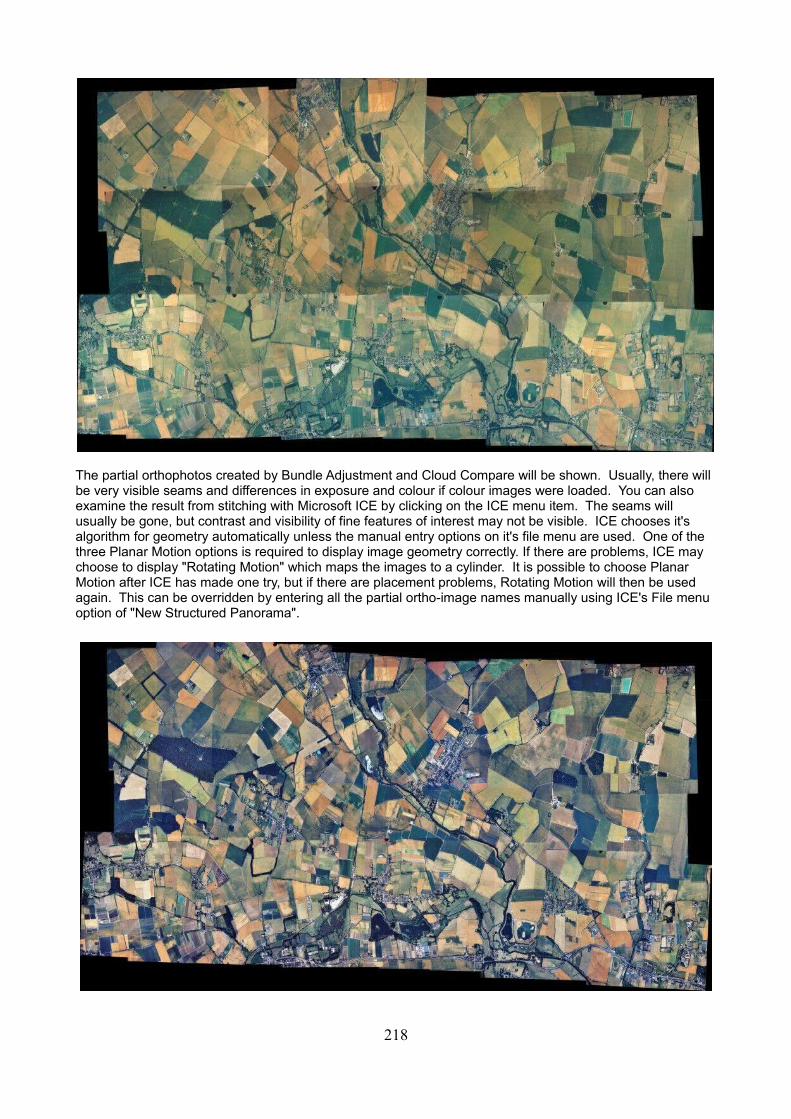
The partial orthophotos created by Bundle Adjustment and Cloud Compare will be shown. Usually, there will be very visible seams and differences in exposure and colour if colour images were loaded. You can also examine the result from stitching with Microsoft ICE by clicking on the ICE menu item. The seams will usually be gone, but contrast and visibility of fine features of interest may not be visible. ICE chooses it's algorithm for geometry automatically unless the manual entry options on it's file menu are used. One of the three Planar Motion options is required to display image geometry correctly. If there are problems, ICE may choose to display "Rotating Motion" which maps the images to a cylinder. It is possible to choose Planar Motion after ICE has made one try, but if there are placement problems, Rotating Motion will then be used again. This can be overridden by entering all the partial ortho-image names manually using ICE's File menu option of "New Structured Panorama".

218

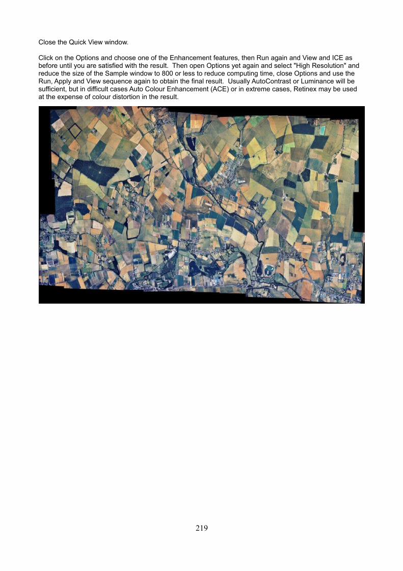
Close the Quick View window.

Click on the Options and choose one of the Enhancement features, then Run again and View and ICE as before until you are satisfied with the result. Then open Options yet again and select "High Resolution" and reduce the size of the Sample window to 800 or less to reduce computing time, close Options and use the Run, Apply and View sequence again to obtain the final result. Usually AutoContrast or Luminance will be sufficient, but in difficult cases Auto Colour Enhancement (ACE) or in extreme cases, Retinex may be used at the expense of colour distortion in the result.

219

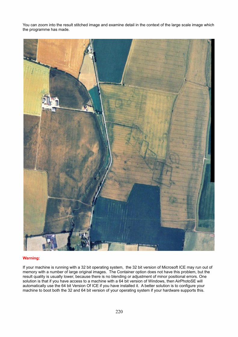
You can zoom into the result stitched image and examine detail in the context of the large scale image whichthe programme has made.

Warning:

If your machine is running with a 32 bit operating system, the 32 bit version of Microsoft ICE may run out of memory with a number of large original images. The Container option does not have this problem, but the result quality is usually lower, because there is no blending or adjustment of minor positional errors. One solution is that if you have access to a machine with a 64 bit version of Windows, then AirPhotoSE will automatically use the 64 bit Version Of ICE if you have installed it. A better solution is to configure your machine to boot both the 32 and 64 bit version of your operating system if your hardware supports this.

220

Layers

Layers are separate images which contain different information from the same area and which you want to merge into a single image showing everything at once.

You can load as many as you wish.

The image on to which all the other images will be superimposed is called the background or zero layer. A background layer image is chosen by clicking on it in a normal AirPhoto window before choosing the layers option so that it gets the Windows focus.

Note:

All images and maps for layering on the background must be calibrated and aligned to the same chosen grid and cropped after alignment to remove any white space which surrounds them. Failure to do this may cause the automatic placement and resizing used in the layering function to place the layer incorrectly.

If no files have been loaded, click on layers to load multiple images to superimpose as layers.

After two calibrated files which may be either images or maps have been loaded, clicking on Layers on the main menu

brings up a special window which enables manipulation of the positions, size and orientation of the images with respect to each other.

221

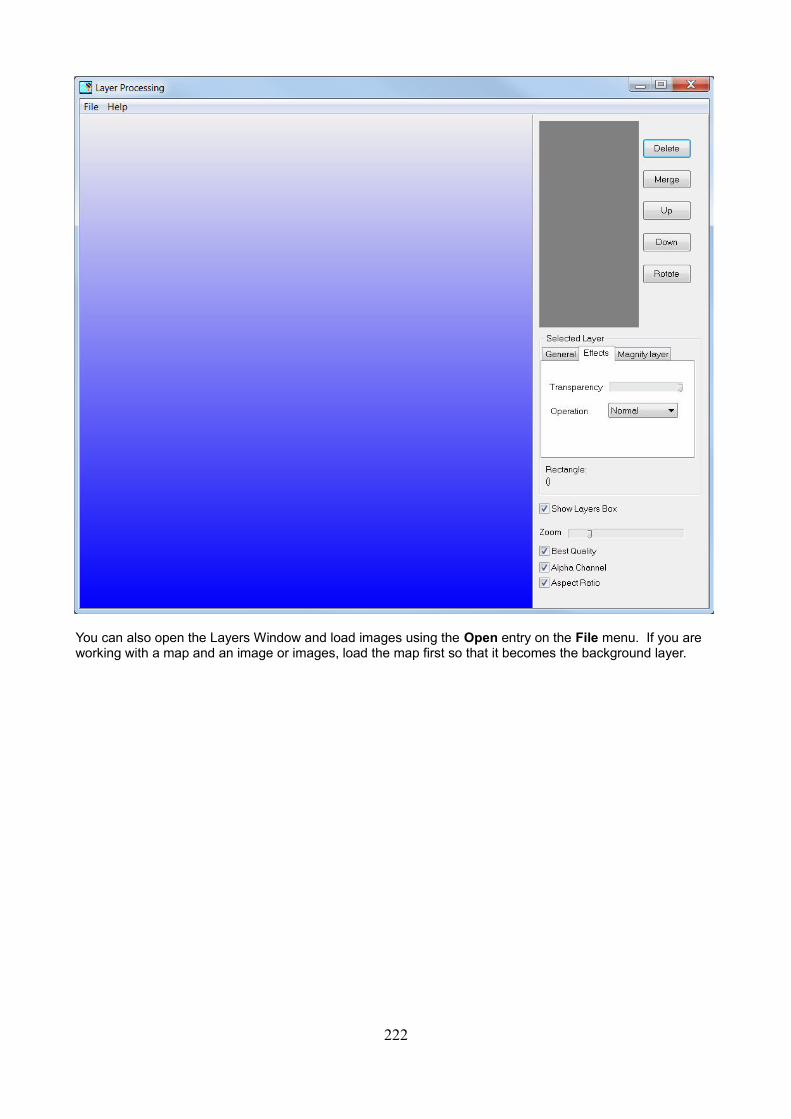
You can also open the Layers Window and load images using the Open entry on the File menu. If you are working with a map and an image or images, load the map first so that it becomes the background layer.

222

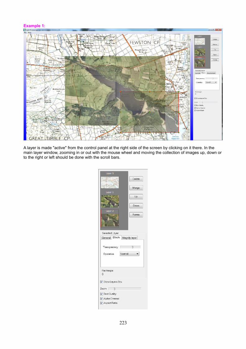
Example 1:

A layer is made "active" from the control panel at the right side of the screen by clicking on it there. In the main layer window, zooming in or out with the mouse wheel and moving the collection of images up, down orto the right or left should be done with the scroll bars.

223

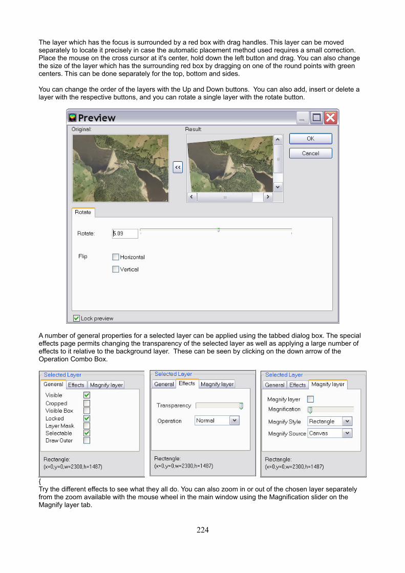
The layer which has the focus is surrounded by a red box with drag handles. This layer can be moved separately to locate it precisely in case the automatic placement method used requires a small correction. Place the mouse on the cross cursor at it's center, hold down the left button and drag. You can also change the size of the layer which has the surrounding red box by dragging on one of the round points with green centers. This can be done separately for the top, bottom and sides.

You can change the order of the layers with the Up and Down buttons. You can also add, insert or delete a layer with the respective buttons, and you can rotate a single layer with the rotate button.

A number of general properties for a selected layer can be applied using the tabbed dialog box. The special effects page permits changing the transparency of the selected layer as well as applying a large number of effects to it relative to the background layer. These can be seen by clicking on the down arrow of the Operation Combo Box.

{Try the different effects to see what they all do. You can also zoom in or out of the chosen layer separately from the zoom available with the mouse wheel in the main window using the Magnification slider on the Magnify layer tab.

224

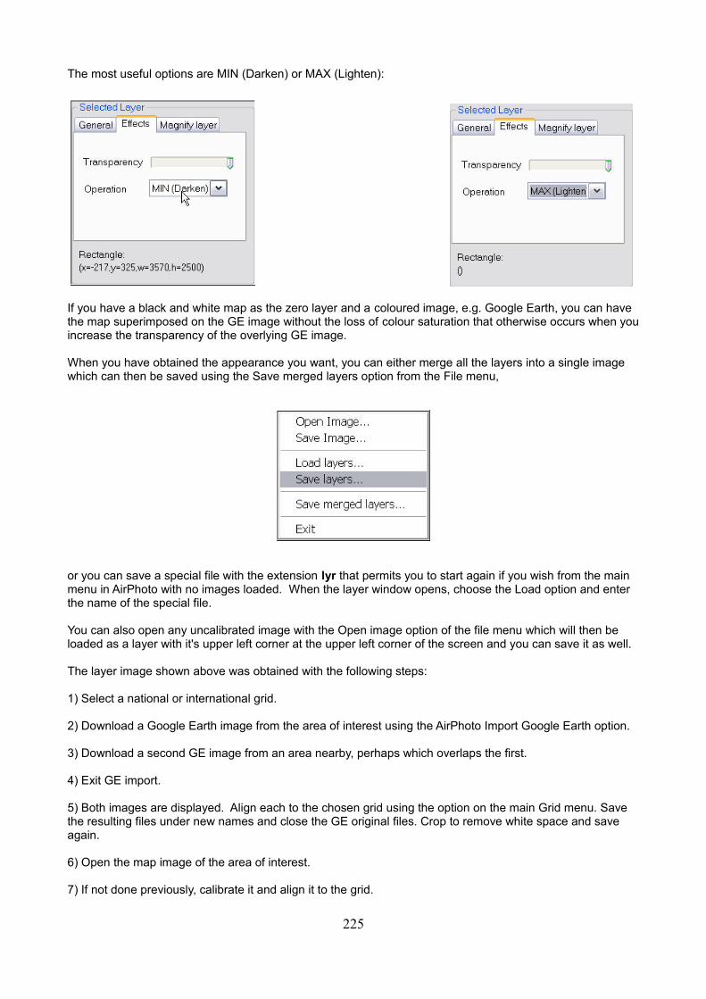
The most useful options are MIN (Darken) or MAX (Lighten):

If you have a black and white map as the zero layer and a coloured image, e.g. Google Earth, you can have the map superimposed on the GE image without the loss of colour saturation that otherwise occurs when youincrease the transparency of the overlying GE image.

When you have obtained the appearance you want, you can either merge all the layers into a single image which can then be saved using the Save merged layers option from the File menu,

or you can save a special file with the extension lyr that permits you to start again if you wish from the main menu in AirPhoto with no images loaded. When the layer window opens, choose the Load option and enter the name of the special file.

You can also open any uncalibrated image with the Open image option of the file menu which will then be loaded as a layer with it's upper left corner at the upper left corner of the screen and you can save it as well.

The layer image shown above was obtained with the following steps:

1) Select a national or international grid.

2) Download a Google Earth image from the area of interest using the AirPhoto Import Google Earth option.

3) Download a second GE image from an area nearby, perhaps which overlaps the first.

4) Exit GE import.

5) Both images are displayed. Align each to the chosen grid using the option on the main Grid menu. Save the resulting files under new names and close the GE original files. Crop to remove white space and save again.

6) Open the map image of the area of interest.

7) If not done previously, calibrate it and align it to the grid.

225

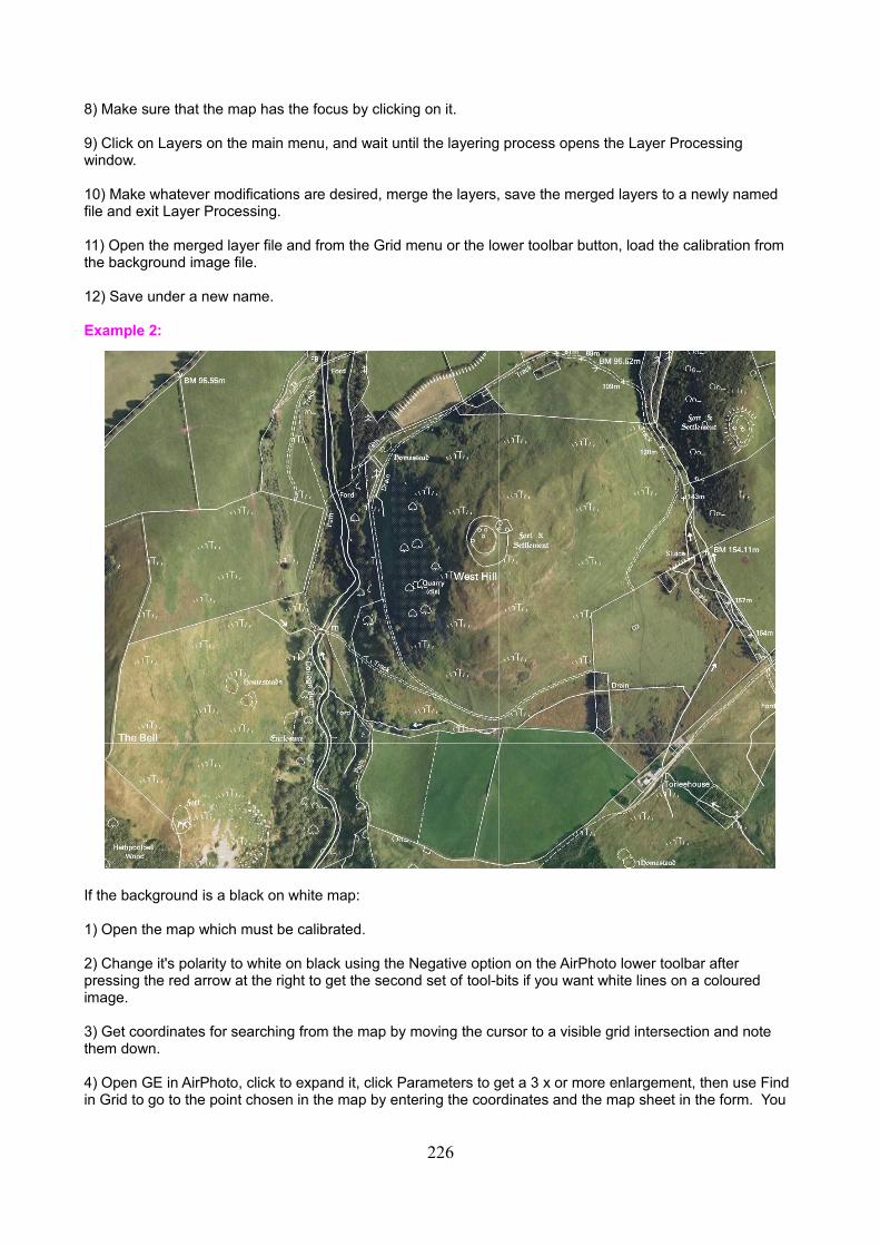
8) Make sure that the map has the focus by clicking on it.

9) Click on Layers on the main menu, and wait until the layering process opens the Layer Processing window.

10) Make whatever modifications are desired, merge the layers, save the merged layers to a newly named file and exit Layer Processing.

11) Open the merged layer file and from the Grid menu or the lower toolbar button, load the calibration from the background image file.

12) Save under a new name.

Example 2:

If the background is a black on white map:

1) Open the map which must be calibrated.

2) Change it's polarity to white on black using the Negative option on the AirPhoto lower toolbar after pressing the red arrow at the right to get the second set of tool-bits if you want white lines on a coloured image.

3) Get coordinates for searching from the map by moving the cursor to a visible grid intersection and note them down.

4) Open GE in AirPhoto, click to expand it, click Parameters to get a 3 x or more enlargement, then use Find in Grid to go to the point chosen in the map by entering the coordinates and the map sheet in the form. You

226

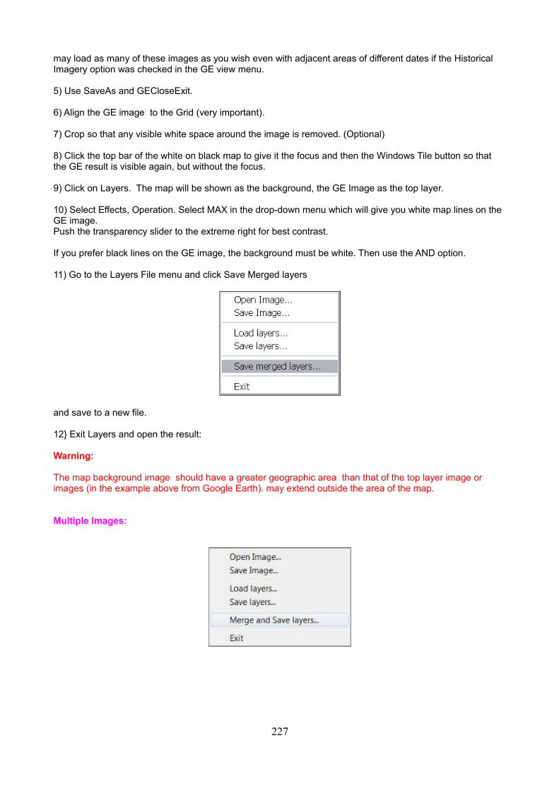
may load as many of these images as you wish even with adjacent areas of different dates if the Historical Imagery option was checked in the GE view menu.

5) Use SaveAs and GECloseExit.

6) Align the GE image to the Grid (very important).

7) Crop so that any visible white space around the image is removed. (Optional)

8) Click the top bar of the white on black map to give it the focus and then the Windows Tile button so that the GE result is visible again, but without the focus.

9) Click on Layers. The map will be shown as the background, the GE Image as the top layer.

10) Select Effects, Operation. Select MAX in the drop-down menu which will give you white map lines on the GE image. Push the transparency slider to the extreme right for best contrast.

If you prefer black lines on the GE image, the background must be white. Then use the AND option.

11) Go to the Layers File menu and click Save Merged layers

and save to a new file.

12} Exit Layers and open the result:

Warning:

The map background image should have a greater geographic area than that of the top layer image or images (in the example above from Google Earth). may extend outside the area of the map.

Multiple Images:

227

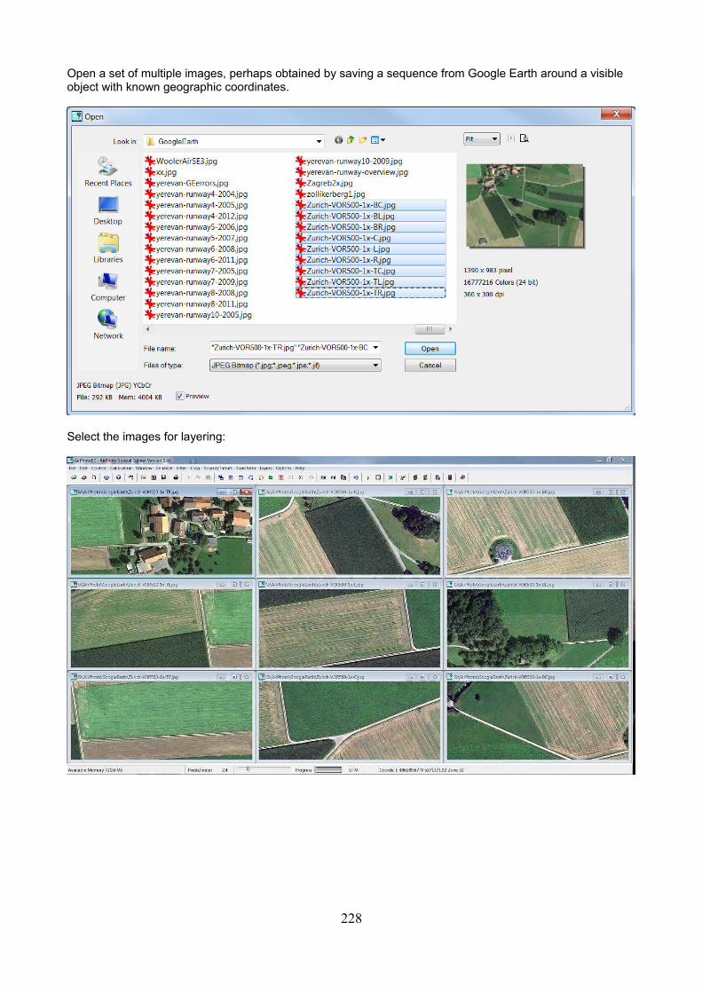
Open a set of multiple images, perhaps obtained by saving a sequence from Google Earth around a visible object with known geographic coordinates.

Select the images for layering:

228

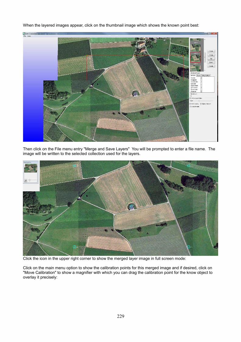
When the layered images appear, click on the thumbnail image which shows the known point best:

Then click on the File menu entry "Merge and Save Layers" You will be prompted to enter a file name. The image will be written to the selected collection used for the layers.

Click the icon in the upper right corner to show the merged layer image in full screen mode:

Click on the main menu option to show the calibration points for this merged image and if desired, click on "Move Calibration" to show a magnifier with which you can drag the calibration point for the know object to overlay it precisely:

229

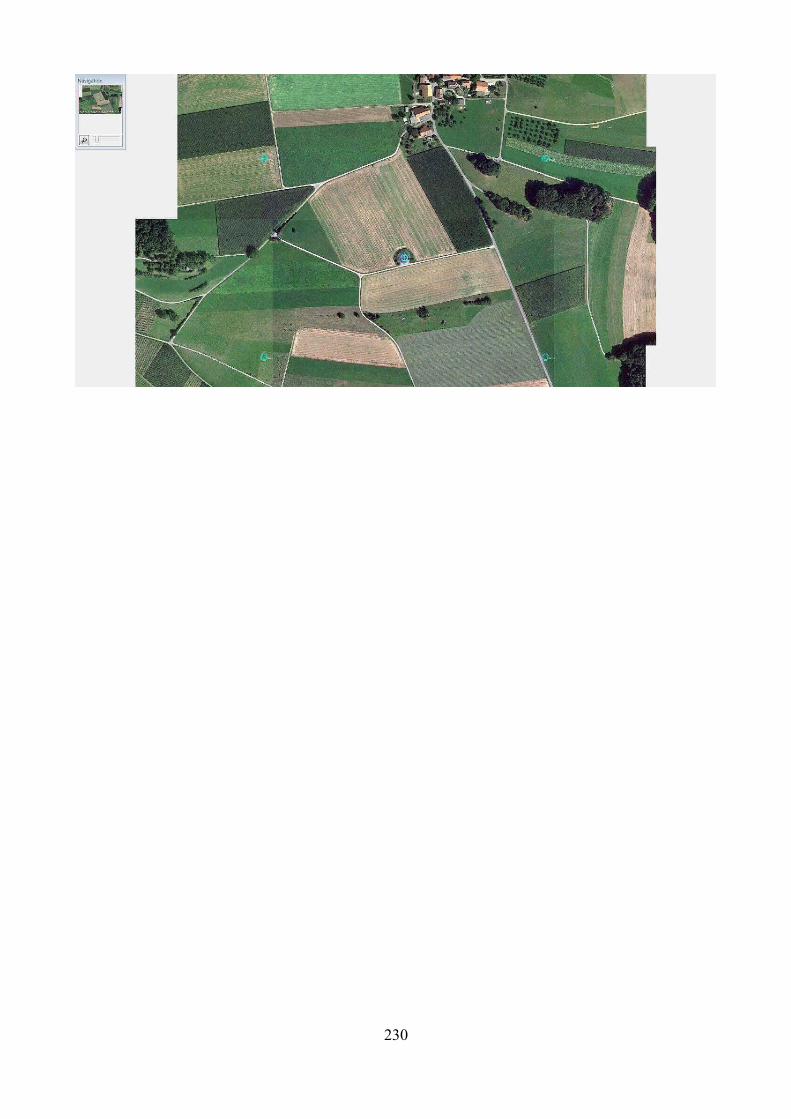
230

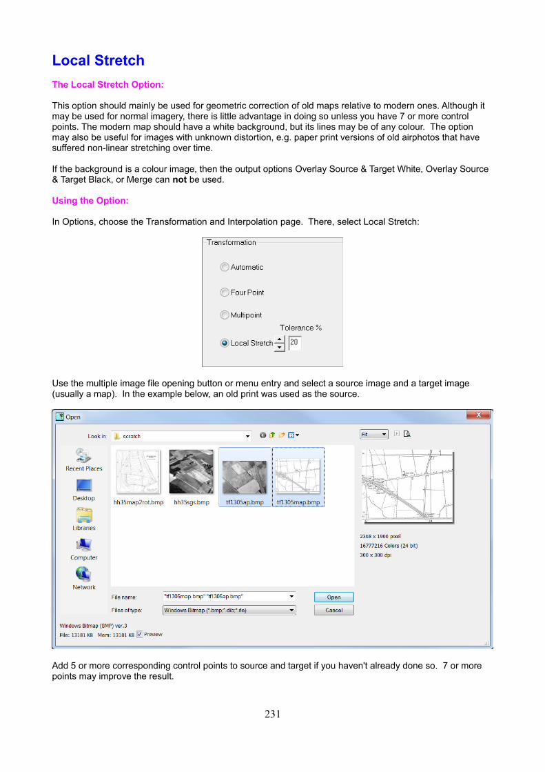
Local Stretch

The Local Stretch Option:

This option should mainly be used for geometric correction of old maps relative to modern ones. Although it may be used for normal imagery, there is little advantage in doing so unless you have 7 or more control points. The modern map should have a white background, but its lines may be of any colour. The option may also be useful for images with unknown distortion, e.g. paper print versions of old airphotos that have suffered non-linear stretching over time.

If the background is a colour image, then the output options Overlay Source & Target White, Overlay Source & Target Black, or Merge can not be used.

Using the Option:

In Options, choose the Transformation and Interpolation page. There, select Local Stretch:

Use the multiple image file opening button or menu entry and select a source image and a target image (usually a map). In the example below, an old print was used as the source.

Add 5 or more corresponding control points to source and target if you haven't already done so. 7 or more points may improve the result.

231

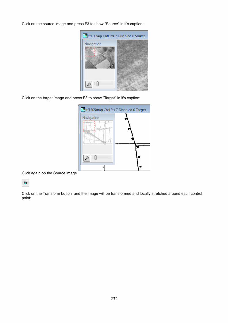
Click on the source image and press F3 to show "Source" in it's caption.

Click on the target image and press F3 to show "Target" in it's caption:

Click again on the Source image.

Click on the Transform button and the image will be transformed and locally stretched around each control point:

232

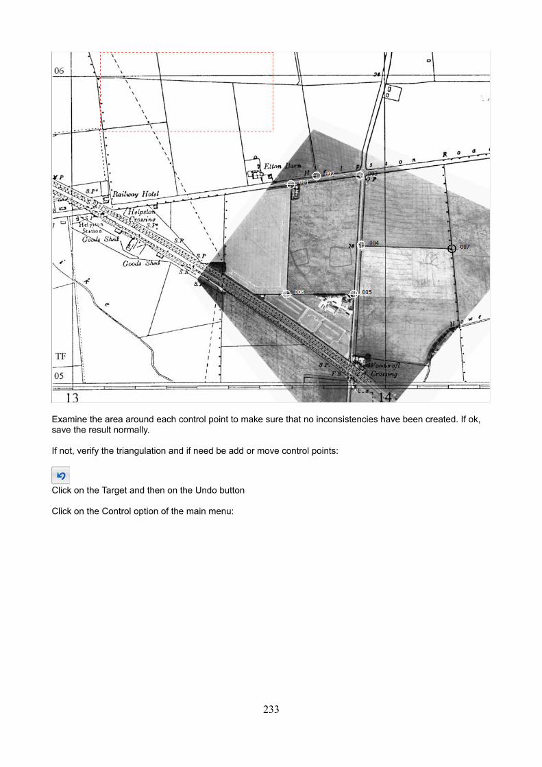
Examine the area around each control point to make sure that no inconsistencies have been created. If ok, save the result normally.

If not, verify the triangulation and if need be add or move control points:

Click on the Target and then on the Undo button

Click on the Control option of the main menu:

233

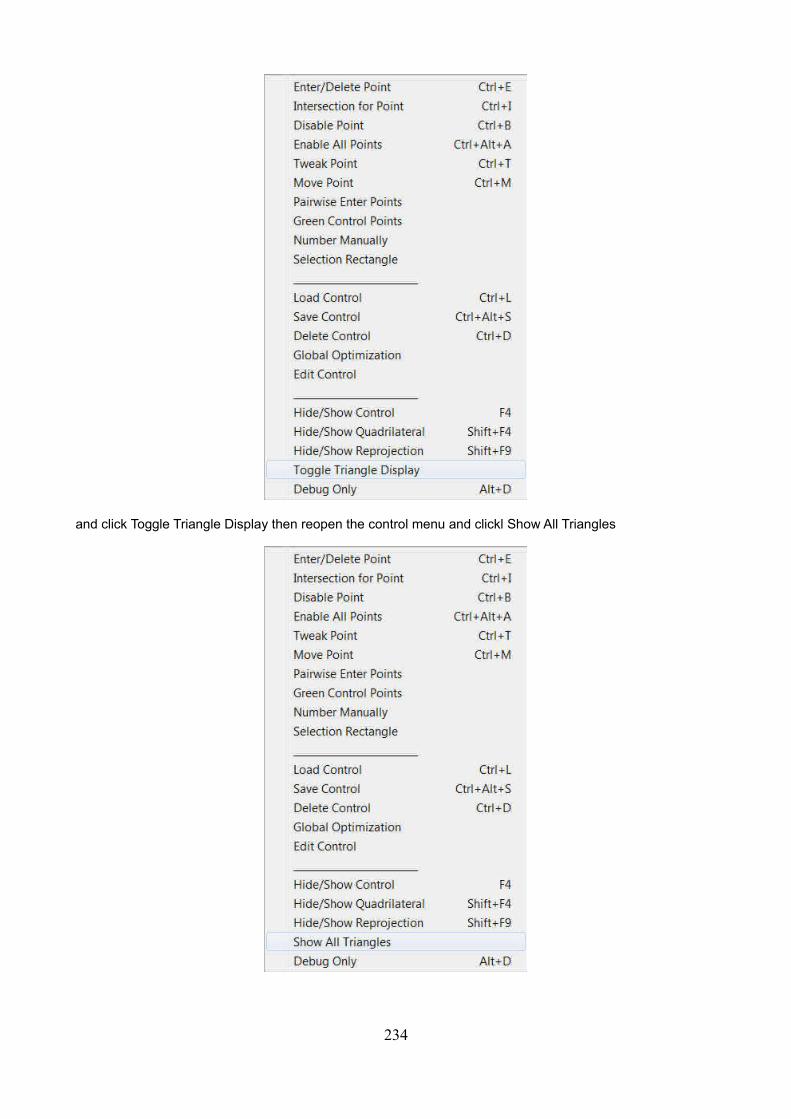
and click Toggle Triangle Display then reopen the control menu and clickl Show All Triangles

234

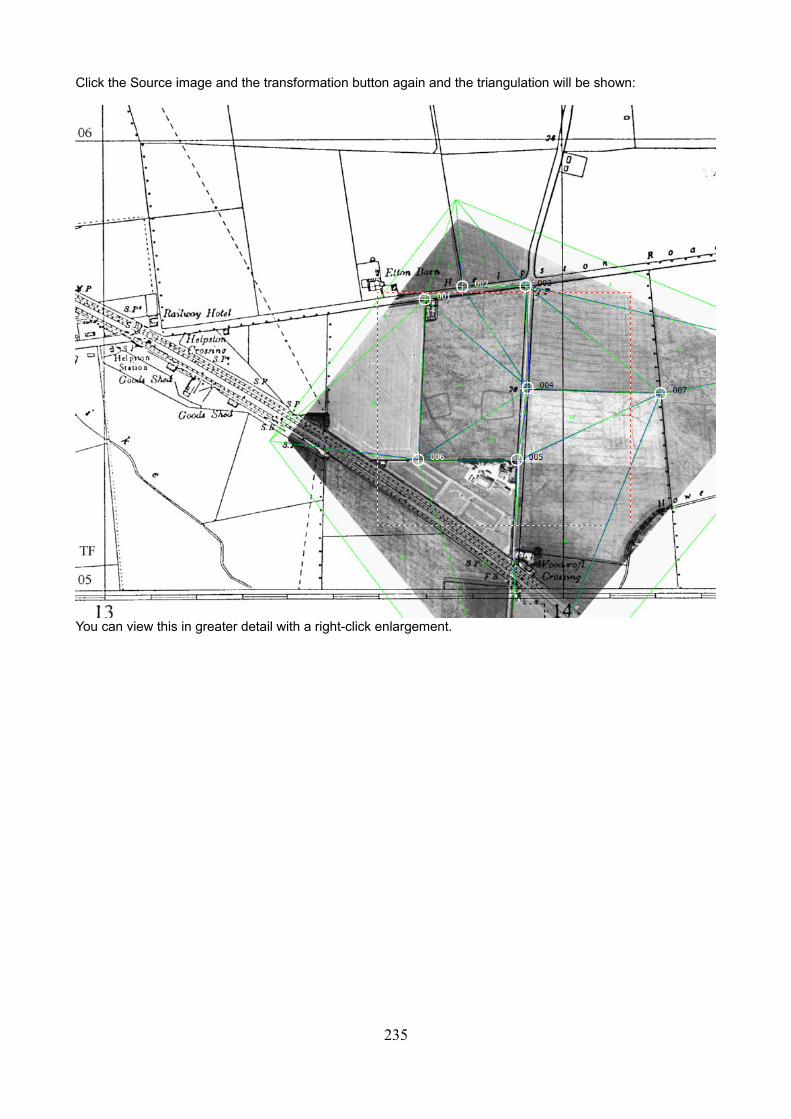
Click the Source image and the transformation button again and the triangulation will be shown:

You can view this in greater detail with a right-click enlargement.

235

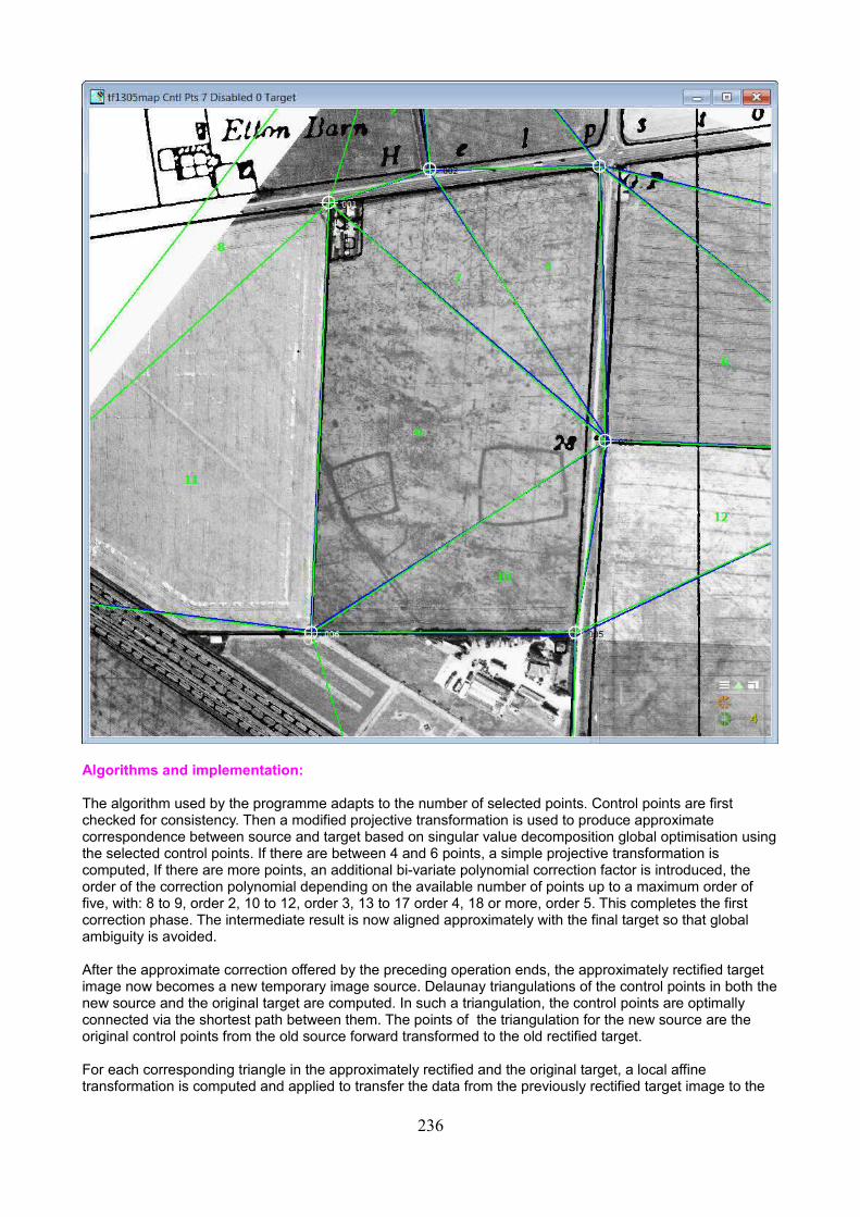
Algorithms and implementation:

The algorithm used by the programme adapts to the number of selected points. Control points are first checked for consistency. Then a modified projective transformation is used to produce approximate correspondence between source and target based on singular value decomposition global optimisation usingthe selected control points. If there are between 4 and 6 points, a simple projective transformation is computed, If there are more points, an additional bi-variate polynomial correction factor is introduced, the order of the correction polynomial depending on the available number of points up to a maximum order of five, with: 8 to 9, order 2, 10 to 12, order 3, 13 to 17 order 4, 18 or more, order 5. This completes the first correction phase. The intermediate result is now aligned approximately with the final target so that global ambiguity is avoided.

After the approximate correction offered by the preceding operation ends, the approximately rectified target image now becomes a new temporary image source. Delaunay triangulations of the control points in both thenew source and the original target are computed. In such a triangulation, the control points are optimally connected via the shortest path between them. The points of the triangulation for the new source are the original control points from the old source forward transformed to the old rectified target.

For each corresponding triangle in the approximately rectified and the original target, a local affine transformation is computed and applied to transfer the data from the previously rectified target image to the

236

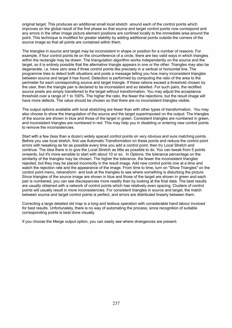
original target. This produces an additional small local stretch around each of the control points which improves on the global result of the first phase so that source and target control points now correspond and any errors in the other image picture element positions are confined locally to the immediate area around thepoint. This technique is modified for greater stability by adding additional points outside the corners of the source image so that all points are contained within them.

The triangles in source and target may be inconsistent in shape or position for a number of reasons. For example, if four control points lie on the circumference of a circle, there are two valid ways in which triangles within the rectangle may be drawn. The triangulation algorithm works independently on the source and the target, so it is entirely possible that the alternative triangle appears in one or the other. Triangles may also bedegenerate, i.e. have zero area if three control points like precisely in a vertical or horizontal line. The programme tries to detect both situations and posts a message telling you how many inconsistent triangles between source and target it has found. Detection is performed by computing the ratio of the area to the perimeter for each corresponding source and target triangle. If these rations exceed a threshold chosen by the user, then the triangle pair is declared to be inconsistent and so labelled. For such pairs, the rectified source pixels are simply transferred to the target without transformation. You may adjust the acceptance threshold over a range of 1 to 100%. The higher the ratio, the fewer the rejections, but the result image will have more defects. The value should be chosen so that there are no inconsistent triangles visible.

The output options available with local stretching are fewer than with other types of transformation. You may also choose to show the triangulation of the source and the target superimposed on the output. The trianglesof the source are shown in blue and those of the target in green. Consistent triangles are numbered in green,and inconsistent triangles are numbered in red. This may help you in disabling or entering new control points to remove the inconsistencies.

Start with a few (less than a dozen) widely spaced control points on very obvious and sure matching points. Before you use local stretch, first use Automatic Transformation on these points and reduce the control point errors with tweaking as far as possible every time you add a control point, then try Local Stretch and continue. The idea there is to give the Local Stretch as little as possible to do. You can tweak from 5 points onwards, but it's more sensible to start with about 10 or so. In Options, the tolerance percentage on the similarity of the triangles may be chosen. The higher the tolerance, the fewer the inconsistent triangles rejected, but they may be placed incorrectly in the result image. Add new control points one at a time and watch the rejection rate and the appearance of the image. From time to time, turn on "Show Triangles" on thecontrol point menu, retransform and look at the triangles to see where something is disturbing the picture. Since triangles of the source image are shown in blue and those of the target are shown in green and each pair is numbered, you can see discrepancies more readily than by looking at the final data. The best results are usually obtained with a network of control points which has relatively even spacing. Clusters of control points will usually result in more inconsistencies. For consistent triangles in source and target, the match between source and target control points is perfect, and errors are distributed linearly between them.

Correcting a large detailed old map is a long and tedious operation with considerable hand labour involved for best results. Unfortunately, there is no way of automating the process, since recognition of suitable corresponding points is best done visually.

If you choose the Merge output option, you can easily see where divergences are present.

237

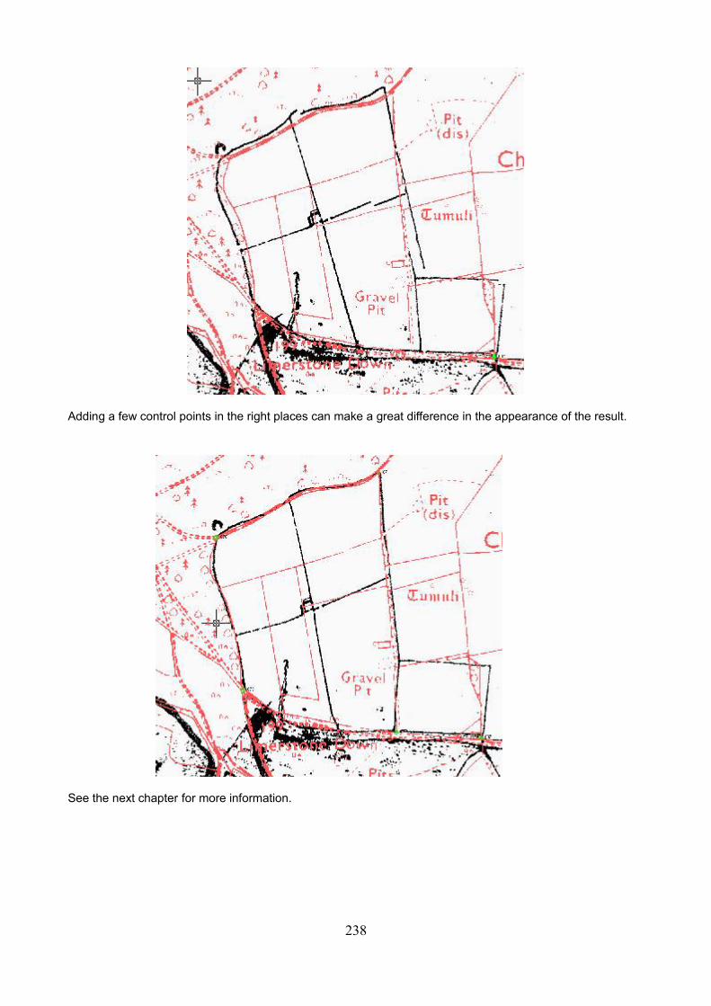
Adding a few control points in the right places can make a great difference in the appearance of the result.

See the next chapter for more information.

238

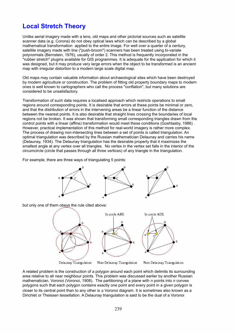
Local Stretch Theory

Unlike aerial imagery made with a lens, old maps and other pictorial sources such as satellite scanner data (e.g. Corona) do not obey optical laws which can be described by a global mathematical transformation applied to the entire image. For well over a quarter of a century, satellite imagery made with line ("push-broom") scanners has been treated using bi-variate polynomials (Bernstein, 1976), usually of order 2. This method is frequently incorporated in the "rubber stretch" plugins available for GIS programmes. It is adequate for the application for which it was designed, but it may produce very large errors when the object to be transformed is an ancient map with irregular distortion to a modern large scale digital map.

Old maps may contain valuable information about archaeological sites which have been destroyed by modern agriculture or construction. The problem of fitting old property boundary maps to modernones is well known to cartographers who call the process "conflation", but many solutions are considered to be unsatisfactory.

Transformation of such data requires a localised approach which restricts operations to small regions around corresponding points. It is desirable that errors at these points be minimal or zero, and that the distribution of errors in the intervening areas be a linear function of the distance between the nearest points. It is also desirable that straight lines crossing the boundaries of local regions not be broken. It was shown that transforming small corresponding triangles drawn from thecontrol points with a linear (affine) transformation would meet these conditions (Goshtasby, 1986) . However, practical implementation of this method for real-world imagery is rather more complex. The process of drawing non-intersecting lines between a set of points is called triangulation. An optimal triangulation was described by the Russian mathematician Delaunay and carries his name (Delaunay, 1934). The Delaunay triangulation has the desirable property that it maximizes the smallest angle at any vertex over all triangles. No vertex in the vertex set falls in the interior of the circumcircle (circle that passes through all three vertices) of any triangle in the triangulation.

For example, there are three ways of triangulating 5 points:

but only one of them obeys the rule cited above:

A related problem is the construction of a polygon around each point which delimits its surrounding area relative to all near neighbour points. This problem was discussed earlier by another Russian mathematician, Voronoi (Voronoi, 1908). The partitioning of a plane with n points into n convex polygons such that each polygon contains exactly one point and every point in a given polygon is closer to its central point than to any other is a Voronoi diagram. It is sometimes also known as a Dirichlet or Theissen tessellation. A Delaunay triangulation is said to be the dual of a Voronoi

239

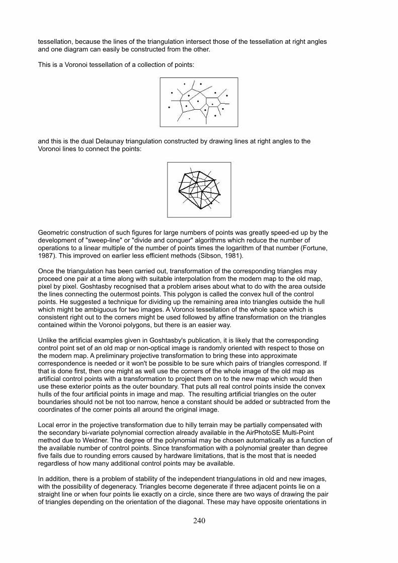
tessellation, because the lines of the triangulation intersect those of the tessellation at right angles and one diagram can easily be constructed from the other.

This is a Voronoi tessellation of a collection of points:

and this is the dual Delaunay triangulation constructed by drawing lines at right angles to the Voronoi lines to connect the points:

Geometric construction of such figures for large numbers of points was greatly speed-ed up by the development of "sweep-line" or "divide and conquer" algorithms which reduce the number of operations to a linear multiple of the number of points times the logarithm of that number (Fortune, 1987). This improved on earlier less efficient methods (Sibson, 1981).

Once the triangulation has been carried out, transformation of the corresponding triangles may proceed one pair at a time along with suitable interpolation from the modern map to the old map, pixel by pixel. Goshtasby recognised that a problem arises about what to do with the area outside the lines connecting the outermost points. This polygon is called the convex hull of the control points. He suggested a technique for dividing up the remaining area into triangles outside the hull which might be ambiguous for two images. A Voronoi tessellation of the whole space which is consistent right out to the corners might be used followed by affine transformation on the triangles contained within the Voronoi polygons, but there is an easier way.

Unlike the artificial examples given in Goshtasby's publication, it is likely that the corresponding control point set of an old map or non-optical image is randomly oriented with respect to those on the modern map. A preliminary projective transformation to bring these into approximate correspondence is needed or it won't be possible to be sure which pairs of triangles correspond. If that is done first, then one might as well use the corners of the whole image of the old map as artificial control points with a transformation to project them on to the new map which would then use these exterior points as the outer boundary. That puts all real control points inside the convex hulls of the four artificial points in image and map. The resulting artificial triangles on the outer boundaries should not be not too narrow, hence a constant should be added or subtracted from the coordinates of the corner points all around the original image.

Local error in the projective transformation due to hilly terrain may be partially compensated with the secondary bi-variate polynomial correction already available in the AirPhotoSE Multi-Point method due to Weidner. The degree of the polynomial may be chosen automatically as a function ofthe available number of control points. Since transformation with a polynomial greater than degree five fails due to rounding errors caused by hardware limitations, that is the most that is needed regardless of how many additional control points may be available.

In addition, there is a problem of stability of the independent triangulations in old and new images, with the possibility of degeneracy. Triangles become degenerate if three adjacent points lie on a straight line or when four points lie exactly on a circle, since there are two ways of drawing the pair of triangles depending on the orientation of the diagonal. These may have opposite orientations in

240

old and new images. Degeneracy can be prevented by using a small random linear transformation on each control point before triangulation as suggested by (Beichl, 2002), but triangles which are inconsistent between old and new images may still result. Occasionally, a triangle may be created in one image which does not exist in the other. A scan through the triangle lists prior to transformation must therefore reorder all entries for correspondence where needed, since the Delaunay algorithm may not create triangles in the same sequence for both sets of points. Furthermore, the vertex coordinates of corresponding triangles may come in any order. By comparing the ratios of the areas to the perimeters of each pair of triangles, remaining inconsistency may be detected. Offering a user-chosen threshold to select those which differ by more than a chosen percentage for separate treatment is then appropriate. A dual pass approach, flagging the consistent triangles in the first pass as 'don't touch', then using only the orientation of the new map triangles for the second pass is a simple solution.

In AirPhotoSE, control points are first checked for consistency. Then a Multi-Point Weidner transformation is used to produce approximate correspondence between source and target using constants determined by Singular Value Decomposition with all control points. If there are between 4 and 6 points, a pure projective transformation) is computed, If there are more, the additional bi-variate polynomial correction described above is introduced, the order of the correction polynomial depending on the available number of points. With 7 to 9 points, order 2 is used, 10 to 12, order 3, 13 to 17 order 4, 18 or more, order 5. This completes the first correction phase.

The set of points in the preliminary image now become a new source and those of the modern mapare used to compute Delaunay triangulations for each. Then for corresponding triangles, an affine transformation is computed and applied to transfer the data from the previously rectified source image to the original modern map. This produces the desired additional small local stretch around each of the control points. Any errors in the other image picture element positions are confined locally to the immediate area around the point.

Several different options for displaying the result are offered, including merging of the lines of the old with the new map where the new has priority over the old, overwriting the new map with the old one leaving other areas unchanged, creating an undistorted version of the old map or mixing the lines both in user-selectable proportions. A diagnostic option is also included to aid with placement of control points. It shows either all the triangles in both images or only those which are inconsistent.

The method may also be used on oblique aerial images if there are a fairly large number (7 or more) of visible control points. This may be used to improve the accuracy of single image rectification if desired.

241

Acknowledgements

Adrien Bartoli at the University of Clermont-Ferrand advised on the mathematics for the methods used and offered many bibliographic references.

Gianluca Cantoro, Institute for Mediterranean Studies, Foundation of Research & Technology Hellas (F.O.R.T.H.) Rethymnon, Crete tested Version 2 and made many helpful suggestions.

Gerald Evenden, USGS, for the PROJ.4 Cartographic Projections library

Yasutaka Furukawa of Google and to Jean Ponce of the Ecole Normale Supérieure for the programme PMVS2

Daniel Girardeau-Montaut, TIMC-IMAG (Grenoble), made additions to his CloudCompare programme at theauthor's request and largely made the orthophoto option possible.

Rafael Grampone von Gioi, Ecole Normale Superiuere (Cashan) for moifications to his code Scons to extractfield boudaries and roads from Google Earth data.

Peter Kovesi of the University of Western Australia, Perth supplied Matlab code to the Oxford web site and corrected a number of bugs at the author's request.

Pierre Moulon, ENPC (Paris), recompiled the code for Bundler and PMVS2 for the Open Source Photogrammetry Toolbox used here.

David M. Mount of the University of Maryland for his ANN (Approximate Near Neighbour) code.

Rog Palmer of AirPhoto Services, Cambridge was of vital help in testing and making many suggestions for improvements to the user interface and the documentation.

Noah Snavely of Cornell University for placing his programme Bundler in source code on the Internet

Maurizio Toscano, University of Grenada, kindly supplied large sets of test data for development and tested the Total Station Transform code.

Fabrizio di Vittorio, Ladispoli, who programmed the HiComponents image processing suite, provided many of the essential tools around which this programme was created.

Frank Warmerdam, Mountain View, California for his additions, revisions and maintenance of PROJ.4.

Andrew Zisserman of the University of Oxford posted Matlab code on the Computer Vision group's web site at my request to illustrate many of the methods described in his book written with Richard Hartley of Australian National University, Canberra .

Lidka Zuk of the University of Poznan made the fruitful suggestion for adding GeoPortal sites to the programme and tested the new features.

242

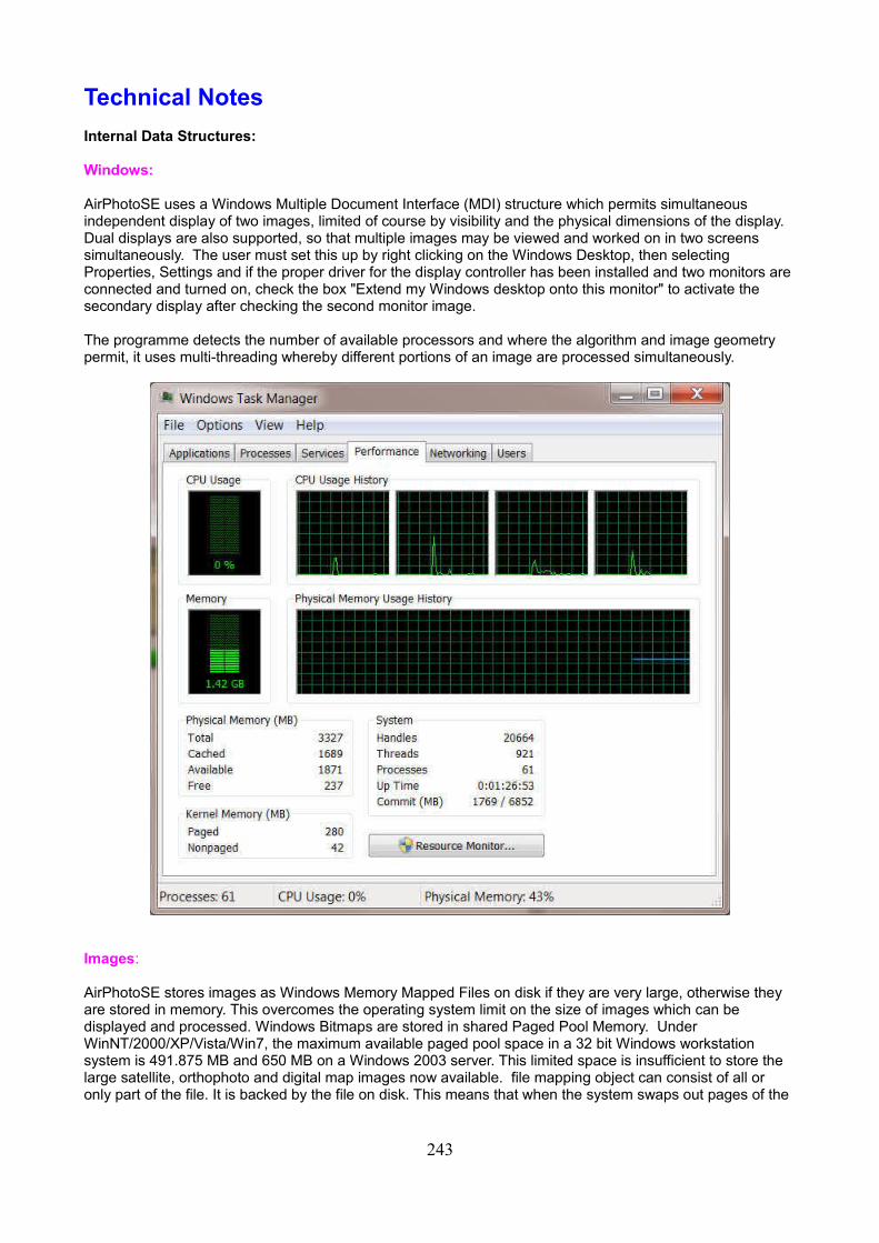
Technical Notes

Internal Data Structures:

Windows:

AirPhotoSE uses a Windows Multiple Document Interface (MDI) structure which permits simultaneous independent display of two images, limited of course by visibility and the physical dimensions of the display. Dual displays are also supported, so that multiple images may be viewed and worked on in two screens simultaneously. The user must set this up by right clicking on the Windows Desktop, then selecting Properties, Settings and if the proper driver for the display controller has been installed and two monitors are connected and turned on, check the box "Extend my Windows desktop onto this monitor" to activate the secondary display after checking the second monitor image.

The programme detects the number of available processors and where the algorithm and image geometry permit, it uses multi-threading whereby different portions of an image are processed simultaneously.

Images:

AirPhotoSE stores images as Windows Memory Mapped Files on disk if they are very large, otherwise they are stored in memory. This overcomes the operating system limit on the size of images which can be displayed and processed. Windows Bitmaps are stored in shared Paged Pool Memory. Under WinNT/2000/XP/Vista/Win7, the maximum available paged pool space in a 32 bit Windows workstation system is 491.875 MB and 650 MB on a Windows 2003 server. This limited space is insufficient to store the large satellite, orthophoto and digital map images now available. file mapping object can consist of all or only part of the file. It is backed by the file on disk. This means that when the system swaps out pages of the

243

file mapping object, any changes made to the file mapping object are written to the file. When the pages of the file mapping object are swapped back in, they are restored from the file. The file view can consist of all oronly part of the file mapping object. A process manipulates the file through the file views. A process can create multiple views for a file mapping object. The file views created by each process reside in the virtual address space of that process. When multiple processes use the same file mapping object to create views for a local file, the data is coherent. That is, the views contain identical copies of the file on disk. The file cannot reside on a remote computer.

Control and Calibration Points:

AirPhotoSE stores control and calibration points for each image object in two self-balancing binary trees. One is indexed on the point ID numbers, the other is indexed on the x-y pixel coordinates.

Each control point in each tree has data stored with a pointer to a record:

PControlPtRecord = ^ControlPtRecord; ControlPtRecord = record Id: Integer; X: Integer; Y: Integer; Z: Integer; CoordX: Extended; CoordY: Extended; CoordZ: Extended; IsEnabled: Boolean; BackgroundBitmap: TIEBitmap; ForegroundBitmap: TIEBitmap; end;

Id is the control point's identification number. X and Y are pixel coordinates of the position of the control pointin the image, Z is a 32 bit integer whose bits are used for specialised flags, e.g. for noting that the coordinates of the control point lie outside the image itself if it has been entered using the line intersection option in control point entry or specifying an EPSG grid number. CoordX, CoordY, and CoordZ are included for compatibility with control point records in AirPhoto where they contain geographic coordinates in decimal latitude, longitude and height above the chosen ellipsoid. In AirPhotoSE all values are zero. IsEnabled is a flag which is turned off if the control point is disabled. The Background Bitmap is a small image of the area where the control point data will be located, copied from location in the memory mapped file window. The Foreground Bitmap is the same area with the control point number and symbol written over the background image data. This is copied to the memory mapped file to display a control point. To hide a control point, the background is copied instead. If an image is rotated, scaled, or transformed, all control point images are first rendered invisible by copying all backgrounds for all points to the memory mapped file window. Then, after the operation is completed, the backgrounds and then the foregrounds are refreshed at all the image points with appropriate orientation changes if required.

Calibration points are stored with a similar record:

PCalPtRecord = ^CalPtRecord; CalPtRecord = record Id: Integer; X: Integer; Y: Integer; Z: Integer; CoordX: Extended; CoordY: Extended; CoordZ: Extended; IsEnabled: Boolean; CalCoordinates: CoordinateType; BackgroundBitmap: TIEBitmap; ForegroundBitmap: TIEBitmap; end;

244

except for the addition of the coordinate type variable which specifies the grid coordinates. WGS84-UTM, Decimal Longitude/Latitude and arbitrary X-Y coordinates are available. Coordinate types for points in a given image may not be mixed. GIS input and output is supported for ArcGis and MapInfo. However, X-Y coordinates are not available for GIS output in MapInfo format.

All the records in both trees are streamed to a binary file when either the user specifically request saving control points or optionally when an image is closed. These files have the same name as the image file but with a .ctl extension. They are automatically re-read into the trees when an image object is loaded and the background and foreground bitmaps are re-created and loaded with image data from the referenced points.

Algorithms and hardware:

Image transformation and calibration use SVD (Singular Value Decomposition) for a least-squares implementation with an unlimited number of points for computation of a homography between an image and a map or between the positions of the calibration points and their geographic values.

Speed in making orthophotos is achieved by automatic computation of keypoints for matching on a reduced size version of each image, the degree of reduction being under user control. The original images are rectified and applied to a terrain model computed from a point cloud created with the help of bundle adjustment.

Control Point Algorithms:

A minimum of four control points in a source and target (map, satellite, geoportal image) is required to establish correspondence. The main rectification algorithm used by the programme adapts automatically to the number of points entered. A modified projective transformation is used to produce approximate correspondence between source and target based on Singular Value Decomposition least squares optimisation

If there are between 4 and 6 points, a pure projective transformation is computed, If there are more, additional bi-variate polynomial correction factors are introduced, the order of the correction polynomial depending on the available number of points up to a maximum order of five (Scollar et al. 1990), with: 7 to 9, order 2, 10 to 12, order 3, 13 to 17 order 4, 18 or more, order 5. The relative quality of the transformation is obtained by computing the differences between forward and inverse transformation at each control point (Reprojection Error, displayed with Shift-F9). Higher order corrections aid in reducing the effects of radial lens distortion, atmospheric refraction and hilly terrain.

The Google Earth and the GeoPortal Viewers:

AirPhotoSE uses the Delphi wrapper TWebBrowser around the Microsoft Windows dynamic link library shdocvw.dll. Details are given at:

https://www.google.com/earth/outreach/tutorials/importgis.html

It is also used in the Internet Explorer from version 4.0 onward. In turn, the AirPhotoSE code for Google Earth calls a JavaScript programme GEDemo.htm which manages Google Earth's GEPlugin and interfaces itto the WebBrowser environment. GEDemo.htm is created afresh each time Google Earth is loaded in AirPhotoSE to permit any changes in the display format which may have been made to be used. The Shdocvw.dll defaults to Internet Explorer version 7. This may result in an error message reporting that the web browser is out of date from a site if it checks the browser version and finds that a version later than 7 is required. The problem can be overcome with the UseIE menu item in AirPhotoSE's GeoPortal implementation.

Warning:

If a registry change is made to force the use of a later version of the Internet Explorer with AirPhotoSE to prevent error messages coming from a GeoPortal website, then the JavaScript used to run Google Earth may fail and Google Earth may not open. Unfortunately, no way has been found to prevent this incompatibility.

245

Orthophoto and Point Cloud Generation:

Orthophotos from multiple images are created with a series of separate programmes which are spawned from AirPhotoSE. When a 64 bit version of Windows is detected, an optimized 64 bit version is used to permit processing of a large number of images.

Keypoint Detection:

Keypoint (salient points) are detected using code written by Andrea Vedaldi. The VLFeat open source library implements popular computer vision algorithms including HOG, SIFT, MSER, k-means, hierarchical k-means,agglomerative information bottleneck, SLIC superpixels, and quick shift. It is written in C for efficiency and compatibility

http://www.vlfeat.org/

This contains a much improved and augmented version of the SIFT algorithm due to David Lowe:

http://www.cs.ubc.ca/~lowe/keypoints/

Approximate Nearest Neighbor Searching:

The ANN library by David M. Mount and Sunil Arya is used for creating a list of keypoint nearest neibhbour keypoints.

http://www.cs.umd.edu/~mount/ANN/

Bundle Adjustment:

Bundle adjustment using the keypoint neighbour lists is carried out with code written by Noah Snavely

http://www.cs.cornell.edu/~snavely/bundler/bundler-v0.3-manual.html

to create a Stanford 3D PLY file.

http://graphics.stanford.edu/data/3Dscanrep/

It in turn uses the code of the sparse Bundle Adjustment package of Lourakis and Argyros

M.I.A. Lourakis and A.A. Argyros. The Design and Implementation of a Generic Sparse Bundle Adjustment Software Package Based on the Levenberg-Marquardt Algorithm. Tech. Rep. 340, Inst. of Computer Science-FORTH, Heraklion, Crete, Greece. Available from

http://www.ics.forth.gr/~lourakis/sba

Point Clouds:

If a Point Cloud is desired, the output from Bundle adjustment is refined using the algorithms CMVS and PMVS2 written by Yasutaka Furukawa:

http://www.di.ens.fr/cmvs/

as programmed for 32 and 64 bit Windows by Pierre Moulon:

http://francemapping.free.fr/Portfolio/Prog3D/CMVS.html

in a version from the Open Source Photogrammetry library:

http://opensourcephotogrammetry.blogspot.de/search?updated-min=2013-01-01T00:00:00-08:00&updated-max=2014-01-01T00:00:00-08:00&max-results=1

246

Cloud Compare:

The PLY output from Bundle adjustment or the Point Cloud is used to create orthophotos from each image and if chosen, a digital terrain model is made using the program Cloud Compare by Daniel Girardeau Montaud:

http://www.danielgm.net/cc/

It offers a huge variety of additional treatments for point clouds which it spawns in turn.

Stitching:

Rough image stitching is done using output of the corner coordinartes of the orthophoto quadrilaterals created in Cloud Compare and with blending and secondary position adjustment using Microsoft's ICE by Matt Uyttendaele and team:

http://research.microsoft.com/en-us/um/redmond/groups/ivm/ice/

Richard Szeliski, Simon Winder, and Matt Uyttendaele, High-quality multi-pass image resampling, no. MSR-TR-2010-10, February 2010

http://research.microsoft.com/pubs/119069/msr-tr-2010-10c.pdf

Programming:

AirPhotoSE was programmed in Delphi 2010 by Irwin Scollar using the ImageEn libraries of Fabrizio Di Vittorio from

http://www.imageen.com/

for many low-level image functions.

It also uses many routines from the Turbo Power libraries:

http://sourceforge.net/users/tpsfadmin

Routines from the JEDI Code Library and JEDI Visual Component libraries:

http://www.delphi-jedi.org/

are also widely used.

247

Bibliography

A complete bibliography for the methods of computer vision behind this programme would have many tens ofthousands of entries. Many of these references can be found on the Internet and a large number of published papers can be downloaded in PDF format.

The fundamental work is Richard Hartley and Andrew Zisserman's Multiple View Geometry in computer vision, Cambridge University Press 2003, Second Edition, ISBN 0521 54051 8

See also:

http://www.robots.ox.ac.uk/~vgg/is the link to the Oxford University Computer Vision Group's web site offering Matlab code which has been ported to Borland Delphi 7 for use in this programme. The code itself can be found at:

http://www.robots.ox.ac.uk/~vgg/hzbook/code/It also contains some sample chapters of Richard Hartley and Andrew Zisserman's seminal book, "Multiple View Geometry in Computer Vision". The mathematics behind the methods used in this programme can be found there.

Additional code ported to Delphi for creating this programme can be found at Peter Kovesi's site: http://www.peterkovesi.com/matlabfns/index.html

The very extensive Links from the Oxford site offer Web URL's for many of the most important research laboratories working in the field.

Another exhaustive listing of research groups in the computer vision field may be found at:

http://www-cgi.cs.cmu.edu/afs/cs/project/cil/ftp/html/v-groups.html

Adrien Bartoli whose advice on this project was fundamental, has a personal page which may be found at:

http://isit.u-clermont1.fr/~ab/Publications/index.html

It contains copies of his published papers which delve deeply into the methods involved.

Image enhancement and filtering algorithms used in AirPhotoSE:

ACE:

A. Rizzi, C. Gatta, D. Marini, A new algorithm for unsupervised global and local colour correction http://www.dti.unimi.it/rizzi/papers/prl03.pdf

Local Adaptive Contrast (Wallis):

Wallis, R. An approach to the space variant restoration and enhancement of images. Proceedings, Symposium on Current Mathematical Problems in Image Science, Monterey CA, 1976 10-12 reprinted in C.O. Wilde E. Barrett, eds. Image Science Mathematics, Western Periodicals, North Hollywood, CA, 1977.

See also: Equation 10.4-6 in W.K. Pratt, Digital Image Processing, 4th ed. Wiley, p. 289, 2007

http://eu.wiley.com/WileyCDA/WileyTitle/productCd-EHEP000722,descCd-google_preview.html Search for page 289.

Luminance (Meylan):

Meylan, High Dynamic Range Image Rendering with a Retinex-Based Adaptive Filter, http://rr.epfl.ch/12/1/Meylan_TIP2006.pdf

248

Retinex (Land):

K. Barnard and B. Funt, "Investigations into multi-scale retinex," in Colour Imaging: Vision and Technology, pp. 9-17, John Wiley and Sons (1999).http://kobus.ca/research/publications/99/CIVT-99/MSR-book-chapter.pdf

White Balance:

N. Limare, J. L. Lisani, J. M. Morel, A. Belén Petro, C. Sbert, Simplest Colour Balance, Image Processing OnLine http://www.ipol.im/pub/algo/lmps_simplest_color_balance/#index7h1

Edge Extract, Scratch/Dirt Removal, Sharpen:

I. Scollar, B. Weidner, T. S. Huang, Image Enhancement Using the Median and the Interquartile Distance,CVGIP(25), No. 2, February 1984, pp. 236-251. http://www.uni-koeln.de/~al001/Scollar-Weidner-Huang.pdf

Rectification algorithms::

I. Scollar, A. Tabbagh, A. Hesse, I. Herzog, Archaeological Prospecting and Remote Sensing, Cambridge University Press, 1990, ISBN 0 521 32050 X, Chapter 5, 224-242

Local Stretch:

Beichl, I. Dealing with degeneracy in triangulation, Computing in Science & Engineering, 4, 2002, 70-74.

Bernstein, R. Digital image processing of earth observation data, IBM Journal of Research and Development, 20, 1976, 40-57.

Delaunay, B. Sur la sphere vide. A la mémoire de Georges Voronoi, Izv. Bull. Acad. Sci. USSR: Class. Sci. Math. Nat., 7, 1934, 793-800.

Fortune, S. A sweep line algorithm for Voronoi diagrams, Algorithmica 2, 1987, 153-174.

Goshtasby, A. Piecewise linear mapping functions for image registration, Pattern Recognition, 19, 1986, 459-466.

Sibson, R. A brief description of natural neighbour interpolation. Interpreting Multivariate Data, p. 21-36 ed. V. Barnet, Wiley, Chichester, 1981.

Voronoi GF. Nouvelles applications des paramètres continus à la théorie des formes quadratiques. Deuxième Mémoire, Recherche sur les parallélopèdres primitifs. Journal Reine u. Angewandte Mathematik, 1908 134 198-287.

249

Installation Notes

Programs and Plugins:

AirPhotoSE uses a large number of public domain executable programmes. There are two sets of these, one for 32 bit and one for 64 bit versions of the Windows operating system. When the programme starts, thecurrent operating system is detected and recorded for further use. Both sets of external executables are copied by the installation programme to subdirectories of the programme directory, so that there is no need for distributing two versions of AirPhotoSE.

In addition when it starts, the programme checks to see if optional programmes like the Microsoft Image Compositing Editor either in the 64 bit or the 32 bit version and Google Earth are present, and if so, where they are located so that they can be run by AirPhotoSE when required. Installing Microsoft ICE before using it in AirPhotoSE will also install additional packages as required or give instructions on where to get them on the Internet. The programme also checks for the presence of an Internet connection, so that Google Earth and GeoPortal sites can be loaded when required. In addition, if an Internet connection is available, the programme checks itself at 180 day intervals if you haven't updated to the latest version of AirPhotoSE and asks you to do so. You can also update more frequently by clicking on the Help menu sub-item for an update check, so that you won't see a reminder until the 180 day interval has expired.

CloudCompare, which is used for making orthophotos, digital terrain models also has 32 and 64 bit versions. It requires the Visual C++ 2008 Redistributable Package (x86) if your operating system is a 32 bit version of Windows, or the Visual C++ 2010 Redistributable Package (x64) if your operating system is a 64 bit version. Installing other programmes may have installed one or the other of these, but if an error message reporting amissing file is shown when CloudCompare starts, then open:

http://www.microsoft.com/en-us/download/details.aspx?id=29

for the 32 bit version

or

http://www.microsoft.com/en-us/download/details.aspx?id=14632

for the 64 bit version and install one or the other depending on your operating system.

You also need one or both of the following Visual C++ redistributable packages:

32 bit systems

Microsoft Visual C++ 2008 Redistributable Package (x86)

http://www.microsoft.com/en-us/download/details.aspx?id=29

Microsoft Visual C++ 2010 Redistributable Package (x86):

http://www.microsoft.com/en-us/download/details.aspx?id=5555

64 bit systems

Microsoft Visual C++ 2010 Redistributable Package (x64):

http://www.microsoft.com/en-us/download/details.aspx?id=14632

If you get error messages from one of the many spawned programmes concerning missing dynamic link libraries, please consult:

http://www.microsoft.com/en-us/download/search.aspx?q=Redistributable+Package

250

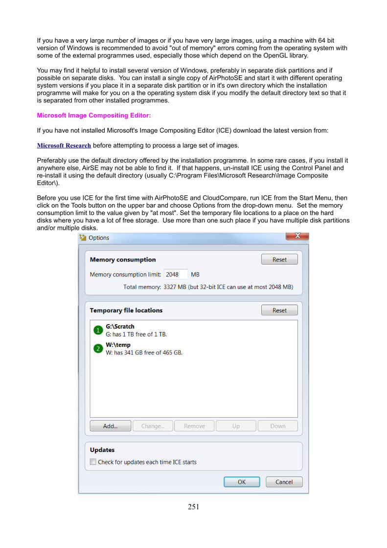
If you have a very large number of images or if you have very large images, using a machine with 64 bit version of Windows is recommended to avoid "out of memory" errors coming from the operating system with some of the external programmes used, especially those which depend on the OpenGL library.

You may find it helpful to install several version of Windows, preferably in separate disk partitions and if possible on separate disks. You can install a single copy of AirPhotoSE and start it with different operating system versions if you place it in a separate disk partition or in it's own directory which the installation programme will make for you on a the operating system disk if you modify the default directory text so that it is separated from other installed programmes.

Microsoft Image Compositing Editor:

If you have not installed Microsoft's Image Compositing Editor (ICE) download the latest version from:

Microsoft Research before attempting to process a large set of images.

Preferably use the default directory offered by the installation programme. In some rare cases, if you install it anywhere else, AirSE may not be able to find it. If that happens, un-install ICE using the Control Panel and re-install it using the default directory (usually C:\Program Files\Microsoft Research\Image Composite Editor\).

Before you use ICE for the first time with AirPhotoSE and CloudCompare, run ICE from the Start Menu, then click on the Tools button on the upper bar and choose Options from the drop-down menu. Set the memory consumption limit to the value given by "at most". Set the temporary file locations to a place on the hard disks where you have a lot of free storage. Use more than one such place if you have multiple disk partitionsand/or multiple disks.

251

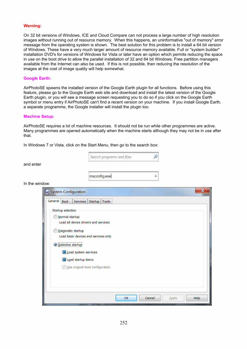
Warning:

On 32 bit versions of Windows, ICE and Cloud Compare can not process a large number of high resolution images without running out of resource memory. When this happens, an uninformative "out of memory" errormessage from the operating system is shown. The best solution for this problem is to install a 64 bit version of Windows. These have a very much larger amount of resource memory available. Full or "system builder" installation DVD's for versions of Windows for Vista or later have an option which permits reducing the spacein use on the boot drive to allow the parallel installation of 32 and 64 bit Windows. Free partition managers available from the Internet can also be used. If this is not possible, then reducing the resolution of the images at the cost of image quality will help somewhat.

Google Earth:

AirPhotoSE spawns the installed version of the Google Earth plugin for all functions. Before using this feature, please go to the Google Earth web site and download and install the latest version of the Google Earth plugin, or you will see a message screen requesting you to do so if you click on the Google Earth symbol or menu entry if AirPhotoSE can't find a recent version on your machine. If you install Google Earth, a separate programme, the Google installer will install the plugin too.

Machine Setup:

AirPhotoSE requires a lot of machine resources. It should not be run while other programmes are active. Many programmes are opened automatically when the machine starts although they may not be in use after that.

In Windows 7 or Vista, click on the Start Menu, then go to the search box:

and enter

In the window:

252

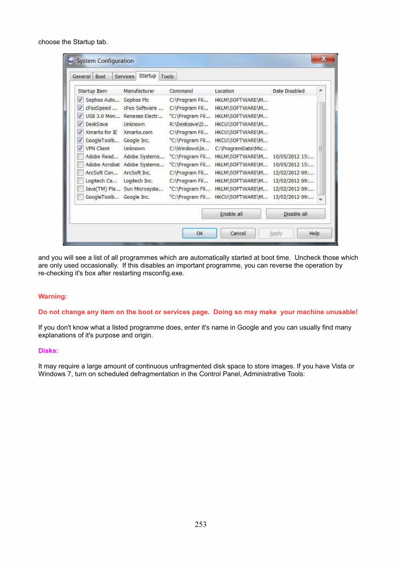
choose the Startup tab.

and you will see a list of all programmes which are automatically started at boot time. Uncheck those which are only used occasionally. If this disables an important programme, you can reverse the operation by re-checking it's box after restarting msconfig.exe.

Warning:

Do not change any item on the boot or services page. Doing so may make your machine unusable!

If you don't know what a listed programme does, enter it's name in Google and you can usually find many explanations of it's purpose and origin.

Disks:

It may require a large amount of continuous unfragmented disk space to store images. If you have Vista or Windows 7, turn on scheduled defragmentation in the Control Panel, Administrative Tools:

253

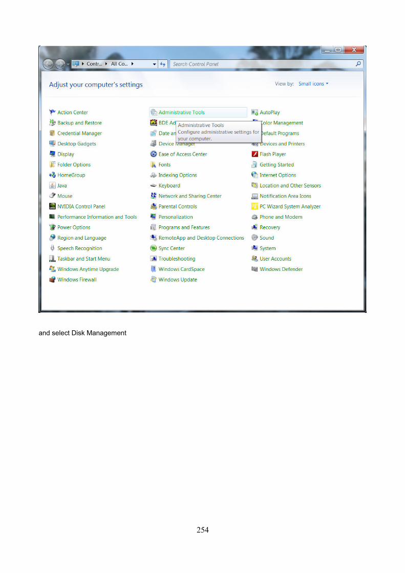
and select Disk Management

254

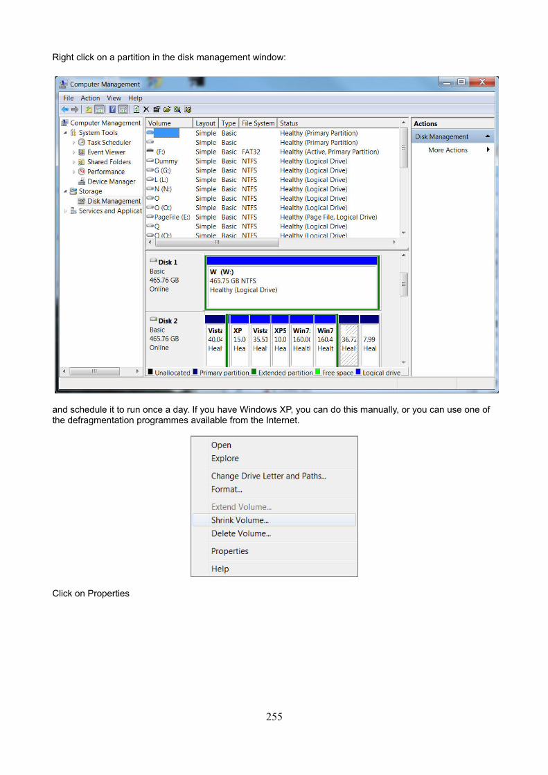
Right click on a partition in the disk management window:

and schedule it to run once a day. If you have Windows XP, you can do this manually, or you can use one of the defragmentation programmes available from the Internet.

Click on Properties

255

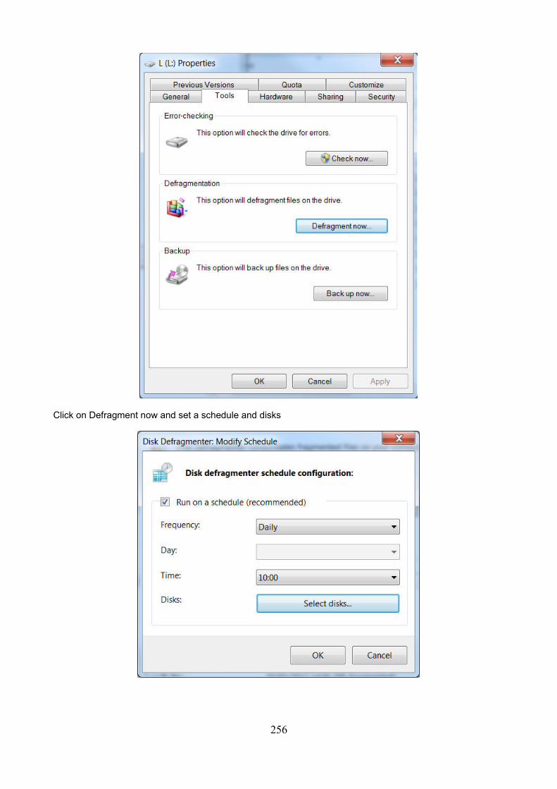
Click on Defragment now and set a schedule and disks

256

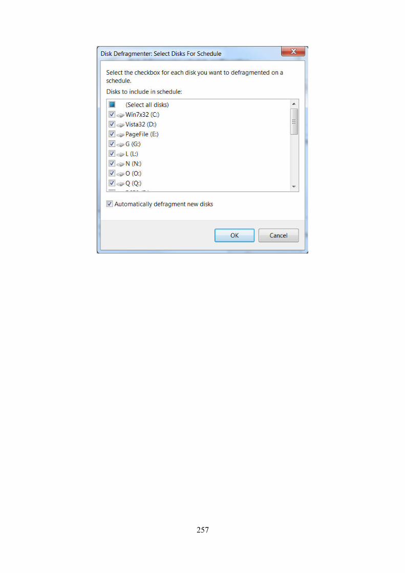
257

New and changed features:

2.67

Changed

There are now three options for Google Earth Pro calibration including lat/lon points, no points and multiple calibration points.

2.66

Changed

All references to the Google Earth Plugin have been removed since it no longer works. Please install GoogleEarth Pro and follow the suggestions in Help.

2.65

New

A function has been added to extract field and road boundaries from images. A black and white line drawing which resembles a map is produced without intervention from a colour or grayscale original. The calibration of the original may be used. The function can be activated on an open image either from the Calibration menu or from a grid-symbol tool button on the main toolbar with a single mouse click.

2.64

Changed

In selection for orthophoto production, directory names with blank spaces and some forbidden ASCII characters like apostrophies could not be processed by the external programmes used, This problem is nowdetected and when present, an option offered to create and copy image data to directories without blank spaces for furtjer processing..

2.63

Bug fix:

When a Google Earth/Pro image was calibrated with EPSG coordinates, these were not shown immediately after a conversion had been made. Fixed.

2.62

New:

A small set of additional image processing options has been added interactive quick modifications.

Changed:

Since 2006, AirPhoto and its successor AirPhotoSE have offered extended options for using Google Earth. Internally, these used the Google Earth Plugin, a separate programme for external control of Google Earth which was installed automatically by Google. From December 15, 2015 Google cancelled support for the Plugin which will no longer run at some time in the near future in recent Windows versions.

Only Google's limited implementation of the Keyhole Markup Language is now available. This language contains a subset of commands to be given to the Google Earth program, but no feedback from the Google server returns data needed for functionality needed the automatic calibration and georeferencing of a Google

258

Earth image which was previously available.

The Google Earth Plugin may continue to work on some machines for an unspecified time. Use it in preference to Google Earth Pro if it works, since it requires less manual intervention.

Google Earth Pro which previously required an annual payment to Google is now available without charge. See the instructions in the Help in the topic Google Earth on how to download, install and configure it. It offers options for higher resolution images than those available with the standard version of Google Earth and without Google advertising labels, but images can only be saved from within Google Earth Pro or with an external screen capture program or operating system option. Modest interaction via the Clipboard has been incorporated in AirPhotoSE to permit transfer of filenames to Google Earth or Google Earth Pro. Both versions may be installed, but only Google Earth Pro will be used from inside AirPhotoSE if it is available.

2.61

Changed:

Many external programmes used by AirPhotoSE fail if blank spaces in file names passed to them are encountered. Additionally, if the user created a folder with blank spaces in it's name for images, this also caused failure when fully qualified path names for images were passed to an external programme...For example, VLfeat detects keypoints in images for orthophoto generation. New versions of VLfeat for 64 and 32 bit systems have replaced older versions, but because it is also written for Linux/Unix, blank spaces in names are still forbidden.

Blank spaces in file or directory names are now filled automatically with the underscore character _ Previousversions of AirPhotoSE required removing all blank spaces in names manually with the Explorer or in a command line window.

2.60

Bug fix:

On fast machines with solid state disks (SSD), the measurement method for calibrated images did not locate the measurement points quickly enough when the mouse was clicked and measurement failed. Fixed.

2.59

Changed:

Microsoft's Image Compositing Editor has been used in AirPhotoSE for several years for stitching orthophotos. A new version 2 has been issued by Microsoft Research after 4 years in 2015. The internal interface for running it from AirPhotoSE had to be modified to utilize the different options for installation offered by Microsoft. At this time however, many users of AirPhotoSE may continue to use the older 2011 version. AirphotoSE has now been modified to detect the version installed and take appropriate action so that the differing installation modes do not prevent finding the executable and spawning it. The images in this help are from the earlier version. These will be modified later.

2.58

Bug fix:

The undo option did not work consistently when Transform and Scale, Clone and Transform or Total Station Transform were chosen. Fixed.

2.57

259

Bug fix:

On some fast new machines with many processors, timing problems interfered with some of the options for Google Earth, namely Test Coordinates, Find in Grid, and Find with GPS information. Fixed.

2.56

New:

Auto-contrast and brightness enhancement are now applied to the thumbnails for the images chosen in the Orthophoto option so that visibility especially in underexposed UAV pictures is improved.

Changed:

An improved detection technique for the installation of Microsoft's Image Compositing Editor now also finds itwhen it is not installed in the default program directory on the C: drive even when the machine has a 64 bit version of Windows running.

2.55

Changed:

A stricter check on image and folder names containing blank spaces has been added to protect spawned external programmes which may operate incorrectly or crash when the Orthophoto option is chosen.

2.54

Changed:

A new revision of Cloud Compare with bug fixes and new features replaces the older version previously used.

2.53

Bug fixes:

A bug was introduced in version 2.48 which disabled simple transformation to a white or black background. Fixed.

The message: "Transformation calculation failed or reset error" sometimes appeared when in fact there was no error. Fixed.

When a second large image was loaded after a first large image was already displayed, the second image sometimes replaced the first and a blank window was shown where the second should have been. Fixed.

If a calibrated (georeferenced) image was aligned to a selected grid and then saved with a new name, no calibration file was written and re-opening the image did not show the grid coordinates. Fixed.

2.52

Bug fixes:

A timing problem affects some Windows 8 machines when Google Earth is being used from within AirPhotoSE. No data was visible in a saved output file. Fixed.

The Altitude slider in the Find in Grid was not visible. Fixed.

Changed:

260

The state of the Find in Grid dialogue box is now recorded to the current user's registry and restored when the programme restarts.

2.51

Bug fix in Enhancement options.

2.50

Bug fixes in the Google Earth "Find by Name" option using Google Maps..

A major revision of Cloud Compare with bug fixes and new features has been integrated into AirPhotoSE.Fortechnical details at the programme development level, see:

Cloud Compare Version 2.5.2

2.49

Changed:

On November 19, 2013, Google withdrew support for Google Maps version 2 which was used for Find by Name searches in AirPhotoSE. The Google Earth placename search code has now been updated to use Google Maps version 3 and to display an area of interest in a separate Google Maps window.

2.48

New:

Local image stretching using affine triangulation has been added as a transformation option. This option is suitable for geometric correction of old maps relative to modern ones or for rectifying scanned paper copies of vertical or oblique images with distortion that can not be modeled mathematically.

Changed:

A new revision of Cloud Compare with bug fixes and new features replaces the older version previously used.

2.47

New:

The polygon crop selection option now permits cropping to an irregular area as well as to the lines between the polygon nodes simply by holding down the left mouse button when tracing the polygon. Data from different years in Google Earth can be activated from AirPhotoSE and selected with the Time Line option, then cropped and inserted into another Google Earth image of differing date using the layer function and passed on to a GIS if the appropriate calibration and GIS world file choices are made first.

2.46

New:

GeoPortal Data: Zooming and spawning of the Internet Explorer

Some GeoPortal sites show a map or orthophoto window which covers only a small part of the display. These can now be expanded by as much as 400% without loss of resolution for large images.

261

Other GeoPortal sites use code which can not be handled by the emulated Web Browser in AirPhotoSE. Forthese sites, a separate version of the latest installed version of the Internet Explorer can now be spawned from the GeoPortal page.

2.45

New:

Layers: Multiple images with automatic calibration

When improving accuracy of calibration of Google Earth images, it may be necessary to extend the area covered by the calibration for points which are distant from a known point. Multiple Google Earth captures around and partly overlapping the known point can be layered and the calibration from the known point transferred automatically to all areas of the larger combined image. See the topic Multiple Images at the bottom of the link above.

2.44

New:

Available transformation projections and interpolation are now offered separately in Options

Projection and interpolation choices in Options set up

Gray-scale images may be converted from negative to positives or the reverse with a single click.

Negative to Positive Images

Measurement of distance, perimiter and polygon area in calibrated images has been added.

Distance, perimeter and area measurement

In addition to trigonometric points, aerial navigation aids which cover most developed countries have well defined coordinates and can be used to aid in calibration of Google Earth images.

Air Navigation Aids for known geographic coordinates

Google Earth image geographic location may have considerable errors. Several methods have been incorporated for reducing these effects.

Improving the accuracy of Google Earth georeferencing

An option for opening multiple images (more than two) has been added to the File Menu, Open Multiple (shortcut key Ctrl-Alt-O). After the image selection dialogue box appears, hold down the Ctrl key and select the images to be opened with the left mouse button. The source and target images must be selected for transformation using the new Source/Target option on the main menu. This multiple image file option is available only if no images have already been opened. For details click on the link above and go to the bottom of the page to the Multiple Files topic.

Transformation image selection

262