1

Algorithmic and Architectural Optimizations forComputationally Efficient Particle Filtering

Aswin C. Sankaranarayanan, Student Member, IEEE, Ankur Srivastava, Member, IEEE,and Rama Chellappa, Fellow, IEEE

Abstract—In this paper, we analyze the computational chal-lenges in implementing particle filtering especially to videosequences. Particle filtering is a technique used for filteringnon-linear dynamical systems driven by non-Gaussian noiseprocesses. It has found wide-spread applications in detection,navigation and tracking problems. Although, in general, particlefiltering methods yield improved results, it is difficult to achievereal time performance. In this paper, we analyze the compu-tational drawbacks of traditional particle filtering algorithms,and present a method for implementing the particle filter usingthe Independent Metropolis Hastings sampler, that is highlyamenable to pipelined implementations and parallelization. Weanalyze the implementations of the proposed algorithm, and inparticular concentrate on implementations that have minimumprocessing times. It is shown that the design parameters for thefastest implementation can be chosen by solving a set of convexprograms. The proposed computational methodology was verifiedover a cluster of PCs for the application of visual tracking.We demonstrate a linear speedup of the algorithm using themethodology proposed in the paper.

Index Terms—Particle Filter, Resampling, MCMC, Auxillaryvariable, Design Methodologies, Visual Tracking

I. INTRODUCTION

Filtering is the problem of estimation of an unknownquantity, usually referred to as state, from a set of observationscorrupted by noise, and has applications to a broad spectrumof real-life problems including GPS navigation, tracking etc.The specific nature of the estimation/filtering problem dependsgreatly on the state we need to estimate, the evolution of thestate with time (if any) and the relation of this state to theobservations and the sources of noise. Generally, analyticalsolutions for estimation are possible in constrained and specialscenarios. For example, Kalman filtering [1] is an optimalanalytic filter when the models are linear and the corruptingnoise processes are Gaussian. For non-linear systems drivenby non-Gaussian processes, the extended Kalman filter or theiterated extended Kalman Filter are used as approximations tothe optimal filtering scheme. Another popular tool for solvingthe inference problems for non-linear systems is particlefiltering [2], [3].

Particle filtering has been applied to a wide variety ofproblems such as tracking, navigation, detection [4], [5] and

A. C. Sankaranarayanan and R. Chellappa are with Center for AutomationResearch and Electrical and Computer Engineering Department, University ofMaryland, College Park, MD - 20742. Email: {aswch,rama}@cfar.umd.edu

A. Srivastava is with Electrical and Computer Engineering Depart-ment, University of Maryland, College Park, MD - 20742. Email:ankurs@glue.umd.edu

This work was partially supported by NSF-ITR Grant 0325119 and a Taskorder from ARL monitored by Alion Science.

video based object recognition. This generality of particlefilters comes from a sample (or particle) based approximationof the posterior density of the state vector. This allows thefilter to handle both the non-linearity of the system as wellas the non-Gaussian nature of noise processes. However,the resulting algorithm is computationally intensive and as aresults, the need for efficient implementations of the algorithm,tuned specifically towards hardware or multi-processor basedimplementations.

Many methods for algorithmic and hardware implementa-tions of particle filtering have been proposed in the literature.The authors of [6] identify resampling algorithms as themain computational step in the algorithm that is completelyindependent of the underlying application. They also proposenew resampling algorithms that reduce the complexity of hard-ware implementations. Architectures for efficient distributedpipelined implementations using FPGAs have been proposedin [7]. A detailed analysis of the basic problem, addressingmany hardware and software issues can also be found in [8],[9].

The resampling algorithms presented in the above referencesare modifications of the basic systematic resampling algorithmpresented in [10], which by itself creates bottle-necks in astreamlined implementation. In [11], the authors propose amethodology to overcome this limitation by rederiving thebasic theory, with an alternate resampling algorithm which issimilar to the Monte Carlo Markov Chain (MCMC) Trackerfor interacting targets in video presented in [12]. There havebeen a number of resampling schemes that have been proposedin the literature. Liu and Chen [13] list and compare a numberof such schemes. Of sufficient interest and relevance are theso called Local Monte Carlo Methods that are described in[13].

A. Motivation

Specifically, this paper analyzes the computational chal-lenges in the implementations of particle filters, and providesa general design methodology for particle filtering usingpipelining and parallelization; these are constructs that arecommonly used in both hardware and multi-processor basedsystems.

Particle filtering involves three main modules: proposition,weight evaluation and resampling modules. Standard imple-mentations of particle filtering typically use what is commonlyknown as systematic resampling (SR). Systematic resamplingposes a significant challenge for pipelined implementations

2

as it can only begin when all the weights are computedat the weight computation stage, and the cumulative sumof the weights is available. This means that any pipelinedimplementation would start the resampling only after all theweights are computed. This increases the latency of the wholeimplementations.

In this paper, we present algorithmic and implementationschemes for particle filters for speeding up the basic com-putations, thereby making particle filtering-based solutionsamenable to real time constraints. We demonstrate a com-putational methodology where the need for the knowledgeof cumulative sum of weights is removed. This implies that,in contrast to traditional particle filtering implementation,the proposed approach does not suffer any bottlenecks inpipelining. Further, this allows us to speedup the filter andreduce its latency through pipelining and parallelization. Wefurther demonstrate the performance of these implementationsusing a cluster of PCs. This allows us to achieve speedups thatare linear in the number of cluster nodes.

B. Specific Contributions

This paper address the computational challenges in hard-ware and multi-processor implementations of particle filters.In this regard, we make the following contributions.

1) Algorithmic Enhancements: In order to avoid the SRstep, we propose the use of the independent MetropolisHastings algorithm [14] for resampling. We show thatthis algorithmic modification is much more amenable topipelining and parallelization.

2) Auxiliary Particle filtering: Further, we show thatmany of the problems associated with the proposedmethodology can be further reduced with the use ofauxiliary particle filters [15]. This allows for completefreedom in the choice of proposal density, which couldbe an important design issue.

3) Minimum Time Implementations: We presentpipeline-able and parallel architectures for implementingthe proposed algorithm. We formulate a set of convexprograms for obtaining the design specification of thefastest implementation of the algorithm. We also provethat given a constraint on the execution speed of thealgorithm, the minimum resources required for theimplementation can be formulated as a convex program.

4) We analyze the pipelining and parallelizability of theproposed implementation using a cluster of PCs fortracking a vehicle in a video stream. We achievespeedups in computation that are linear in the numberof cluster nodes.

The rest of the paper is organized as follows. We firstpresent the traditional particle filtering algorithm in sectionII. In section III, we present the MCMC sampling theory anduse it to propose a computational methodology in Section IV.Section V analyzes the implementations using the proposedmethodology. Finally, in section VI, we demonstrate the per-formance of the proposed implementations for the problem oftracking in videos using a cluster of PCs.

II. PARTICLE FILTERING

In particle filtering, we address the problem of Bayesianinference for dynamical systems. Let X ⊆ R

d and Y ⊆ Rp

denote the state space and the observation space of the systemrespectively. Let xt ∈ X denote the state at time t, and yt ∈ Ythe noisy observation at time t. We model the state sequence{xt} as a Markovian random process. Further we assume thatthe observations {yt} to be conditionally independent giventhe state sequence. Under these assumptions, the system iscompletely characterized by the following:

• p(xt|xt−1): The State transition probability density func-tion, describing the evolution of the system from timet−1 to t. Alternatively, the same could be described witha state transition model of the form xt = h(xt−1, nt),where nt is a noise process.

• p(yt|xt): Observation likelihood density, describing theconditional likelihood of observation given state. Asbefore, this relationship could be in the form of anobservation model yt = f(xt, ωt) where ωt is a noiseprocess independent of nt.

• p(x0): The prior state probability at t = 0.

Given statistical descriptions of the models and noisy ob-servations, we are interested in making inferences about thestate of the system at current time. Specifically, given theobservations till time t, y1:t = {y1, . . . , yt}, we would like toestimate the posterior density function πt = p(xt|y1:t). Withthe posterior, we aim to make inferences I(ft) of the form,

I(ft) = Eπt[ft(xt)] =

∫

ft(xt)p(xt|y1:t)dxt (1)

where ft is some function of interest. An example of such aninference could be the conditional mean, where ft(xt) = xt.

Under Markovian assumption on the state space dynamicsand conditional independence assumption on the observationmodel, the posterior probability is recursively estimated usingthe Bayes Theorem

p(xt|y1:t) =p(yt|xt)

∫

p(xt|xt−1)p(xt−1|y1:t−1)dxt−1

p(yt|y1:t−1)(2)

Note that, there are no unknowns in (2) since all terms areeither specified or computable from the posterior at the previ-ous time step. The problem is that this computation (includingthe integrations) need not have an analytical representation.However, foregoing the requirement for an analytic solution,particle filtering approximates the posterior πt with a discreteset of particles or samples {x

(i)t }N

i=1 with associated weights{w

(i)t }N

i=1 suitably normalized so that∑N

i=1 w(i)t = 1. The

approximation for the posterior density is given by

πt(xt) =

N∑

i=1

w(i)t δxt

(

x(i)t

)

(3)

where δxt(·) is the Dirac Delta function centered at xt. The

set St = {x(i)t , w

(i)t }N

i=1 is the weighted particle set thatrepresents the posterior density at time t, and is estimatedrecursively from St−1. The initial particle set S0 is obtainedfrom sampling the prior density π0 = p(x0).

3

We first discuss the so called importance functiong(xt|xt−1yt), an easy to sample function whose supportencompasses that of πt. The estimation of I(ft), as defined in(1) can be recast as follows,

I(ft) =∫

ft(xt)p(xt|y1:t)

g(xt|xt−1yt)g(xt|xt−1yt)dxt

=∫

ft(xt)w(xt)g(xt|xt−1yt)dxt

(4)

where w(xt) is defined as the so called importance weight,

wt =p(xt|y1:t)

g(xt|xt−1yt)(5)

Particle filters sequentially generate St from St−1 using thefollowing steps,

1) Importance Sampling: Sample x(i)t ∼

g(xt|x(i)t−1yt), i = 1, . . . , N . This step is also called the

proposal step and g(·) is sometimes called the proposaldensity.

2) Computing Importance Weights: Compute the unnor-malized importance weights w

(i)t ,

w(i)t = w

(i)t−1

p(yt|x(i)t )

g(x(i)t |x

(i)t−1yt)

, i = 1, . . . , N. (6)

3) Normalize Weights: Obtain the normalized weightsw

(i)t ,

w(i)t =

w(i)t

∑N

j=1 w(j)t

, i = 1, . . . , N. (7)

4) Inference Estimation: An estimate of the inferenceI(ft) is given by

IN (ft) =N

∑

i=1

ft(x(i)t )w

(i)t (8)

This sequence is performed for each time iteration to getthe posterior at each time step. A basic problem that the abovealgorithm suffers from is that, after a few time steps, all im-portance weights except a few go to zero. These weights willremain at zero for all future time instants (as a result of (6)),and do not contribute to the estimation of IN (ft). Practically,this degeneracy is undesirable and is a waste of computationalresource. This is avoided with the introduction of a resamplingstep. Resampling essentially replicates particles with higherweights and eliminates those with low weights. This can bedone in many ways. [2], [10], [16] list many resamplingalgorithms. The most popular one, originally proposed in [2],samples N particles from the set {x

(i)t } (samples generated

after proposal) according to the multi-nomial distribution withparameters w

(i)t to get a new set of N particles St. The next

iteration uses this new set St for sequential estimation. Wediscuss some additional sampling algorithms in II-B.

A. Choice of Importance Function

Crucial to the performance of the filter, is the choice ofthe importance function g(xt|xt−1yt). Ideally, the importancefunction should be close to the posterior. If we chooseg(xt|xt−1yt) ∝ p(yt|xt)p(xt|xt−1), then we would obtain theimportance weights wt identically equal to 1 and the variance

of the weights would be zero. For most applications, thisdensity function is not easy to sample from. This is largelydue to the non-linearities in the state transition and observationmodels. One popular choice is to use the state transitiondensity p(xt|xt−1) as the importance function. In this case,the importance weights are given by

wt ∝ wt−1p(yt|xt) (9)

Other choices include using cleverly constructed approxi-mations to the posterior density [17].

B. Resampling Algorithms

In the particle filtering algorithm, the resampling step wasintroduced to address degeneracies resulting due to the impor-tance weights getting skewed. Among resampling algorithms,the SR technique is popularly used. The basic steps of SR [16]are recounted below.

• For j = 1, . . . , N

1) Sample J ∼ {1, . . . , N}, such that Pr[J = i] =a(i), for some choice of {a(i)}.

2) The new particle x(j)t = x

(J)t and the associated

weight is w(j)t = w

(J)t /a

(J)t .

• The resampled particle set is St = {x(i)t , w

(i)t }N

i=1.

If a(i) = w(i)t the resampling scheme is the one used in [2].

Other choices are discussed in [16].Particle filtering algorithms that use Sequential Importance

Sampling (SIS) and SR are collectively called SISR algo-rithms. Computationally, SR is a tricky step, as it requiresthe knowledge of the normalized weights. Resampling basedon SR cannot start until all the particles are generatedand the value of the cumulative sum is known. This is thebasic limitation that we overcome by proposing alternativetechniques.

III. INDEPENDENT METROPOLIS HASTINGS ALGORITHM

In this section, we introduce Monte Carlo sampling tech-niques, discuss in detail the Metropolis Hastings Algorithmsand its derivative, the Independent Metropolis Hastings Algo-rithms [14]. Further, we “redesign” the basic particle filteringalgorithm using these techniques for sampling.

Particle filtering is a special case of more general MCMCbased density sampling techniques, specifically suited for dy-namical systems. The Metropolis Hastings Algorithm (MHA)[18], [19] is considered the most general MCMC based sam-pling. Popular samplers such as the Metropolis Sampler [20]or the Gibbs Sampler [21] are special cases of this algorithm.

The MHA and the particle filter both address the issueof generating samples from a distribution whose functionalform is known (upto a normalizing factor) and is difficultto sample. In this section, we present a hybrid sampler thatuses the sampling methodologies adopted in MCMC samplers(specifically, the MHA algorithm) for the problem of esti-mating posterior density functions. We later show that sucha scheme is computationally more favorable than systematicresampling.

4

A. Metropolis Hastings Algorithm

We first present the general theory of MCMC samplingusing the MHA algorithm and then state the conditions un-der which the general theory fits into the particle filteringalgorithm presented before. The MHA generates samplesfrom the desired density (say p(x), x ∈ X ) by generatingsamples from an easy to sample proposal distribution, sayq(x|y), x ∈ X , y ∈ X . MHA produces a sequence of states{x(n), n ≥ 0}, which by construction is Markovian in nature,through the following iterations.

1) Initialize the chain with an arbitrary value x(0) = x0.Here, x0 could be user specified.

2) Given x(n), n ≥ 0, generate x v g(·|x(n)), where g isthe sampling or proposal function.

3) Accept x with probability α(x(n), x) as defined below

α(x(n), x) = min

{

p(x)

p(x(n))

g(x(n)|x)

g(x|x(n)), 1

}

(10)

That is, for a uniform random variable u v U [0, 1]

x(n+1) =

{

x if u ≤ α(x(n), x)x(n) otherwise

(11)

Under mild regularity conditions, it can be shown that theMarkov Chain {x(n)} as constructed by the MHA convergesand has p(x) as its invariant distribution, independent of thevalue x0 chosen to initialize the chain [14].

The MHA is used to generate a Monte Carlo Markov Chainwhose invariant distribution is the distribution p(x). However,there is an initial phase when the chain is said to be in atransient state, due to the effects of the initial value x0 chosen.However, after sufficient samples, the effect of the startingvalue diminishes and can be ignored. The time during whichthe chain is in a transient state is referred to as burn-in period.This is usually dependent on both the desired function p(x),the proposal function q(x|y) and most importantly, on theinitial state x0. In most cases, an estimation of this burn-in period is very difficult. It is usually easier to make aconservative guess of what it could be. There are heuristicsthat estimate the number of burn-in samples (say Nb). Samplesthat are in the burn-in period are discarded.

B. Independent Metropolis Hastings Algorithm

The Independent Metropolis Hastings Algorithm (IMHA)is a special case of the general MHA where the proposalfunction q(x|y) is set as q(x). This makes the proposalfunction independent of the previously accepted sample in thechain. This would mean that the acceptance probability (10)α(x(n), x) of a proposal x ∈ X with the chain at x(n) ∈ X ,

α(x(n), x) = min

{

p(x(n))

g(x(n))

g(x)

p(x), 1

}

(12)

The IMH algorithm has strong convergence properties. Un-der mild regularity conditions, it has been shown to convergeat a uniform rate independent of the value x0 used to initialize

the chain. A study of such convergence properties can be foundin [14], [22].

Both IMHA and SISR are algorithms designed to generatesamples according to a probability density function, with theSISR suited specifically to the sequential nature of dynamicalsystems. In this regard, the the key difference between theIMHA and the SISR algorithm lies in the fact that theSISR algorithm requires the knowledge of cumulative sumof weights (the term

∑N

j=1 w(j)t in (7)). This is important as

the cumulative sum can only be computed when the weightscorresponding to the whole particle set is known. Hence,SR can only begin after all particles are generated and theirweights are computed. In contrast, the IMHA poses no suchbottlenecks. In the next section, we exploit this property todesign a filter that does not suffer from the bottle-necksintroduced by SR.

IV. PROPOSED METHODOLOGY

The bottlenecks introduced by the SR technique can beovercome by using the IMHA for resampling. However, thereare some basic issues that needs to be resolved before weachieve this. To begin with, the generation of particles usingimportance sampling works differently for the two algorithms.Particle filtering allows for the importance function to bedefined locally for each particle. Mathematically, the ith par-ticle at time t is generated from an importance function,represented as g(xt|x

(i)t−1yt), parametrized by x

(i)t−1. This poses

a problem in the application of IMHA to estimate the posterior,because the concept of importance functions associated witheach particle does not extend to IMHA. In contrast, theMHA algorithm requires the importance function to dependfunctionally only on the last accepted sample in the chain, andin the case of the IMHA, the importance function remains thesame.

Given a set of unweighted samples {x(i)t−1, i = 1, . . .}

sampled from the posterior density p(xt−1|y1:t−1) at time t−1,we can approximate the posterior by

p(xt−1|y1:t−1) ≈1

N

N∑

i=1

δxt−1(x

(i)t−1) (13)

where δxt−1(·) is the Dirac Delta function on xt−1. Using (2)

and (13), we can approximate the posterior at time t,

p(xt|y1:t) ≈p(yt|xt)

p(yt|y1:t−1)

1

N

N∑

i=1

p(xt|x(i)t−1) (14)

Sampling from this density can be performed using MHAor IMHA. The issue of choice of importance function nowarises. The importance function typically reflects and exploitsthe knowledge of application domain or could be a cleverapproximation to the posterior. For this reason, we wouldlike to reuse the importance function corresponding to theunderlying model.

Keeping this in mind, we propose a new importance func-tion of the form,

g′(xt|yt) =

N∑

i=1

1

Ng(xt|x

it−1yt) (15)

5

Note that g′(xt|y1:t) qualifies to be an importance functionfor use in IMHA, given its dependence on only one statevariable. To sample from g′(xt|yt), we need to first sampleI v U [1, 2, . . . , N ], and then sample from g(·|xI

t−1yt). Thesampling of I can be done deterministically given the ease ofsampling from uniform densities over finite discrete spaces.Finally, although the new importance function is functionallydifferent from the one used in the SISR algorithm, the gener-ated particles will be identical.

The overall algorithm proceeds similar to IMHA. Wefirst propose particles using the new importance functiong′(xt|y1:t). The acceptance probability now takes the form

α(xt, x) = min

{

w′(x)

w′(xt), 1

}

(16)

w′(xt) = p(yt|xt)

∑Ni=1 p(xt|x

(i)t−1)

∑N

i=1 g(xt|x(i)t−1yt)

(17)

Further, if the choice of the importance function werethe same as the state transition model, i.e, g(xt|xt−1yt) =p(xt|xt−1), then the acceptance probability becomes a ratioof likelihoods,

α(x(n)t , x) = min

{

p(yt|x)

p(yt|x(n)t )

, 1

}

(18)

We can now avoid the systematic resampling of traditionalparticle filtering algorithms. The intuition is that we will useIMHA to generate unweighted particle set/stream from thedesired posterior.

As before, we have an unweighted particle set St−1, thatcontains particles approximating the posterior at time t − 1,πt−1(xt−1). We aim to estimate an approximation to theposterior at time t. As before, the algorithm is initialized withS0 containing samples from the prior p(x0). The main stepsare stated below:

• Importance Sampling (step 1): Generate N + Nb in-dices J(i), i = 1, . . . , N + Nb uniformly from the set{1, 2, 3, . . . , N}, where Nb is an estimate of the burn inperiod and N is the number of particles required. between1..N with uniform density.

• Importance Sampling (step 2): From the particle setSt−1 = {x

(i)t−1, i = 1, . . . , N} at time t−1, propose N +

Nb particles to form the set St = {x(i)t , i = 1, . . . , N +

Nb} using the rule:

x(i)t v g(·|x

J(i)t−1yt) (19)

• Compute Importance Weights: For each particle in St,evaluate the importance weights w′(i)

t , for each i using(17).

• Inference: Estimate the expected value of functions ofinterest. Compute

It(ft) =

∑N+Nb

i=1 f(x(i)t )w′(i)

t∑N+Nb

i=1 w′(i)t

(20)

Note that samples discarded during burn-in can still beused in the computation of (20) as the unnormalized

particle set {x(i)t , w′(i)

t , i = 1, . . . , N + Nb} is stillproperly weighted (when normalized) [23].

• MCMC Sampler: Use the IMH sampler to parsethrough the set St, to generate a new unweighted set ofparticles using the following steps.

1) Initialize the chain with x(1)t = x

(1)t the first particle

proposed.2) for i = 2, . . . , N + Nb,

x(i)t =

{

x(i)t , with prob. α(x

(i−1)t , x

(i)t )

x(i−1)t , with prob. 1 − α(x

(i−1)t , x

(i)t )

(21)where α(·, ·) is the acceptance probability as definedin (10).

Discarding the first Nb samples for burn in, the remainingN samples form St = {x

(i)t , i = Nb + 1, . . . , N}, the

approximation of p(xt|y1:t).

We can now compare the algorithm given above withthe classical SISR discussed in Section II. Note that theSISR algorithm involves a weight normalization step (equation(7)). However, the proposed algorithm works with ratios ofunnormalized weights and requires no such normalization.This allows for the following advantages in the proposedmethodology:

• The IMH sampler works with ratios of importanceweights. This obviates the need for knowledge of nor-malized importance weights, as we can work with unnor-malized weights. This allows the IMH sampler to startparsing through the particles as they are generated, andnot wait for the entire particle set to be generated andthe importance weights computed.

• In contrast, in SISR, the resampling can begin only whenall particles are generated and the cumulative sum ornormalized weights are known.

The ability to resample particles as they are generated allowsfor faster implementations. This is analyzed further in sectionV.

A. Drawbacks of the proposed Framework

The proposed framework overcomes the drawbacks of theSISR algorithm by adopting an MCMC sampling strategyas opposed to the traditional SR technique. However, thenew framework does introduce extra computations that addto increased overall complexity. We discuss these drawbacks,and an alternate formulation that can circumvent this issue.

Consider the expression for weight computation, givenin (17). The expression involves computing the summations∑N

i=1 p(xt|x(i)t−1) and

∑N

i=1 g(xt|x(i)t−1yt), which require ad-

ditional computation time. The computation of both terms doesnot present a severe bottleneck, as it can be easily pipelined.Further, when the proposal density matches the state transitionmodel, the terms cancel each other out.

Nonetheless, it is possible to circumvent this problem usingthe auxiliary particle filtering paradigm [3], [15].

6

B. Auxiliary Particle Filters

Auxiliary particle filtering refers to techniques that extendthe state space of the problem to include a particle index.Consider the new state space {xt, k}, where k ∈ [1, . . . , N ]denotes the particle index. The posterior p(xtk|y1:t) is definedas

p(xtk|y1:t) ∝ p(yt|xt)p(xt|xkt−1) (22)

Marginalizing (22) over the state k gives the expression in(14) for p(xt|y1:t).

Let us further assume that we sample the joint space usinga proposal g(xtk|xt−1yt), i.e, (x

(i)t , k(i)) ∼ g(·|xt−1yt). The

unnormalized weights can be constructed as

w(i)t =

p(yt|x(i)t )p(x

(i)t |xk(i)

t−1)

g(x(i)t , k(i))|x

(i)t−1yt)

(23)

As before, we can resample using an MCMC chain, andthe expression for acceptance probability remains the ratioof unnormalized weights as given in (10). At the inferencestep, we first marginalize across the particle index state k.However, it is easy to see that the marginalization is identicalto discarding the particle index information at each particle,given the nature of the particle-based representation of theunderlying density. In a nutshell, the use of auxiliary variableallows us to completely avoid the summation of (17) and theassociated computational cost.

Finally, there exist many choices for the proposal densityin the extended state space. A discussion on this can be foundin [15].

V. IMPLEMENTATION BASED ON PROPOSED

METHODOLOGY

In this section, we present approaches for implementingthe theory presented in section III. We assume that the basiccomputational blocks for importance sampling, computationof importance weight and parsing of particles as per the IMHalgorithm are available. We use these blocks to propose threeimplementations: a sequential implementation and two parallelimplementations.

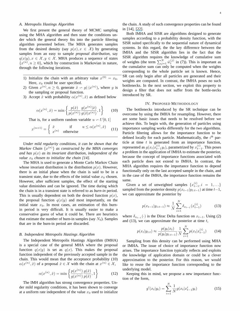
A. Sequential Implementation

Weight Calc St

Estimation BlockExpected Inference

Proposal IMH ChainSt−1

Fig. 1. Sequential Implementation

Figure 1 illustrates a straight-forward implementation of theproposed algorithm. It consists of the following blocks.Proposal Block: The proposal block takes St−1, the particlesfrom the previous time step and proposes new particles x

(i)t

(one particle at a time) by sampling the proposal function.For the IMHA-based algorithm, this amounts to generatinga uniform number J(i) ∼ U [1, 2, . . . , N ] to randomly pick

one particle from St−1, say {xJ(i)t−1}. The particle x

(i)t is

obtained from sampling g(xt|xJ(i)t−1yt). We assume that this

blocks proposes particle one at a time. When we use theauxiliary variable framework, this involves sampling both thestate x

(i)t and the associated particle index state k(i) from a

proposal function g(xtk|xt−1yt).Weight Calculator: This block is an implementation of (17)(or (23) when we use auxiliary variables).IMH Chain: This block is an implementation of (16) in whichthe acceptance probability α is calculated for the new particleand the previously accepted particle. Further, an uniformrandom-number u ∼ U [0, 1] is generated and if it is smallerthan α then the new particle is retained in St, else the lastaccepted particle in the chain is replicated once more.Inference Estimation Block: This block estimates the infer-ence function (equation 1). The computation can be performedin parallel with the IMH chain, and has no effect on the overallcomputation.

The characteristics of this basic implementation are asfollows.

• Sequential Processing of Particles: Each block in theimplementation processes one particle at a time. So, toprocess Q particles each block needs to run Q times.Note that, if we need to generate N particles to representthe posterior density, then we will have to iterate N +Nb

times where Nb is the burn-in period. The last N particlesin the IMH chain is the sample set St.

• Pipelining: By pipelining the blocks, processing in eachblock can be made to overlap in time, leading to anoverall increase in the throughput of the system.

• Computation Time: We now estimate the time requiredto process Q = N + Nb particles under this implemen-tation. Let us suppose that the target application is suchthat the proposal block can generate one particle every Tp

time units. The weight computation block generates theweight of a particle in Tw time units, and the IMH chainprocess particles once in every Td time units. Further, weassume that the overall time required to process is notconstrained by the inference block (and therefore ignoredin this analysis). Under this setting, we can compute thetotal time required to process Q particles.

The implementation in Figure 1 will take Tp + Tw + Td

time units to produce the first particle x(1t ). Thereafter, it

will be able to produce one particle every max(Td, Tp, Tw)time units. The total latency for generating Nb + N particleswould be (Nb + N − 1)max(Td, Tp, Tw) + Tp + Tw + Td

time units. This basic sequential implementation can be madefaster by replicating the proposal, weight computation andthe IMH chain blocks. In order to exploit the parallelismin processing of particles, we present a refinement of thesequential implementation.

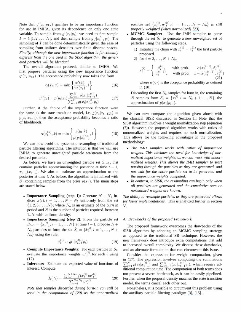
B. Parallel Implementation: Single Chain

Figure 2 illustrates the parallel implementation of theproposed algorithm. We still retain a single IMH Chain,though the proposal and the weight computation blocks arereplicated. Having multiple IMH chains introduces additional

7

Weight Calc

Weight Calc

Weight Calc

Weight Calc

Inference

StSt−1

BU

FFE

R

BU

FFE

R

Proposal

Proposal

IMHA ChainProposal

Fig. 2. Parallel Implementation with a single IMH Chain.

issues involving burn-in in each chain. For this reason, we firstrestrict ourselves to single chain implementations. We relaxthis restriction later in Section V-C. Let the number of proposalblocks be Rp and the number of weight computation blocksbe Rw. We would like to compute the total time requiredto process Q particles as a function of Rp and Rw (and thelatency of the blocks Tp, Tw and Td). Further, we would liketo choose specific values of Rp and Rw to achieve the smallesttotal processing time.

The total computational time is determined by bottlenecksin processing created due to differing rates of processingof particles at each stage. The rate at which the proposalblocks process particles is Rp/Tp, the weight computationblocks at Rw/Tw and the IMHA blocks at 1/Td. The totalcomputational time is predominantly dependent on which ofthe three rates is the smallest.

1) Case A: Rp/Tp ≤ Rw/Tw ≤ 1/Td. : In this scenario,the proposal blocks have the smallest rate of processing,followed by the weight computation blocks. Suppose we needto process Q particles, then the proposal blocks by themselveswill need (Q/Rp)Tp time units to process all particles. Theweight computation and IMHA processing happen in parallel.Given the quicker processing rate at both weight computationand IMHA, by the time the last set of Rp particles is processedat the proposal blocks, all earlier particles have already beenprocessed through the weight computation blocks. The amountof time required to process the last set of Rp particlesat the weight computation blocks and the IMHA block isRpTw/Rw +RwTd. Allowing Rp and Rw to take values overthe real line (and not just positive integers) the total time forprocessing τA is,

τA(Rp, Rw) =Q

Rp

Tp +Rp

Rw

Tw + RwTd (24)

We are now interested in computing the values of Rp andRw that minimize τA, keeping in mind that such solutionsmust satisfy the assumptions of Case A. To begin with, wenote that both Rp and Rw take positive values. This allows anatural change of coordinate frames of the form,

Rp = log(Rp)

Rw = log(Rw)(25)

In terms of Rp and Rw, the expression for τA can be writtenas,

τA(Rp, Rw) = QT−Rp

P + TweRp−Rw + TdeRw (26)

The constraints for the minimization come from the assump-tions made on the ordering of the rates in Case A.

Rp − Rw − log(

Tp

Tw

)

≤ 0

Rw − log(

Tw

Td

)

≤ 0(27)

Finally, Rp and Rw are naturally bounded by the value ofQ. This leads a convex optimization problem with inequalityconstraints stated as,

minRp,RwτA(Rp, Rw) = QTpe

−Rp + TweRp−Rw + TdeRw

(28)

Rp − Rw − log(

Tp

Tw

)

≤ 0 Rp − log Q ≤ 0

Rw − log(

Tw

Td

)

≤ 0 Rw − log Q ≤ 0(29)

We now note that the expression for τA is convex in bothRp and Rw. Further, the inequality constraint is also convexin Rp and Rw. One can use a host of techniques [24] designedspecifically for convex optimization.

2) Case B: Rw/Tw ≤ Rp/Tp, Rw/Tw ≤ 1/Td.: Usinga line of reasoning identical to Case A, we can derive anexpression for the amount of time τB needed to process Qparticles, as a function of Rp and Rw.

τB(Rp, Rw) =Rw

Rp

Tp +Q

Rw

Tw + RwTd (30)

We note that a value of Rp greater than Rw is impracticalleading to a constraint on Rp of the form Rp ≤ Rw. As before,we can recast the set of equations in terms of Rp and Rw (asdefined in (25)) to get the cost and constraint equations.

minRp,RwτB(Rp, Rw) = Tpe

Rw−Rp + QTwe−Rw + TdeRw

(31)

Rw − Rp − log(

Tw

Tp

)

≤ 0 Rw − log Q ≤ 0

Rw − log(

Tw

Td

)

≤ 0 Rp − Rw ≤ 0(32)

Both the cost function and the inequality constraints areconvex in Rp and Rw.

3) Case C: Rp/Tp ≤ 1/Td ≤ Rw/Tw.: In Case C, themain bottleneck is in the proposal block, followed by theIMH chain. Accordingly, the total time τC for processing ofQ particles is

τC(Rp, Rw) =Q

Rp

Tp + Tw + RpTd (33)

8

Using the transformation of variables in (25), we can writedown expressions for both the cost τC and the constraints.

minRp,RwτC(Rp, Rw) = QTpe

−Rp + TweRp−Rw + TdeRw

(34)Rp − Rw − log

(

Tp

Tw

)

≤ 0 Rp − log Q ≤ 0

Rw − log(

Tw

Td

)

≤ 0 Rw − log Q ≤ 0(35)

As before, both the cost and the inequality constraints areconvex over Rp and Rw.

4) Case D: 1/Td = min(Rp/Tp, Rw/Tw, 1/Td).: The finalscenario is when the main bottleneck is at the IMH chain. Theexpression for total time τD is given as,

τD(Rp, Rw) = Tp + Tw + QTd (36)

τD is not dependent on the choice of Rp and Rw. So thewhole feasibility set forms the solution set when we optimizefor minimum processing time. For completeness, we againformulate it as a convex program with the following cost andconstraints.

minRp,RwτD(Rp, Rw) = Tp + Tw + QTd (37)

−Rp + log(

Tp

Td

)

≤ 0 Rp − log Q ≤ 0

−Rw + log(

Tw

Td

)

≤ 0 Rw − log Q ≤ 0(38)

As stated above, in Case D all points in the feasible setform the solution set.

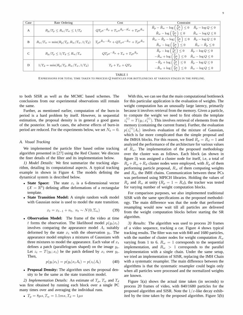
Depending on the exact location of the bottle neck, it ispossible to have upto 6 different scenarios. However, some ofthese scenarios collapse to identical expressions for the totalcost leading to the four cases A through D discussed above.The expressions for the cost and the associated constraints aresummarized in Table I. We note that each case results in aconvex cost function and convex inequality constraints. Thisallows us to design an algorithm for determining the globalminima for total computation time for processing Q particlesgiven values of Tp, Tw and Td.

1) Given values of Td and Tw, formulate FOUR convexprograms associated with the four cases illustrated inTable I.

2) Solve each convex program to obtain minimum timesτi,min, i ∈ {A,B,C,D} and associated values of Rp

and Rw.3) Choose the configuration that gives the least total pro-

cessing time.

The above algorithm allows us to obtain design specifica-tions with minimum processing time given values of Tp, Tw,Td and Q. Note that the basic computation tools used areoptimization techniques for convex programs. Convex opti-mization is a well studied problem, and there are techniquesthat solve convex programs very efficiently and reliably [24].Further, convex programs have very desirable properties withrespect to local minima. All local minima are also globalminima, and further the set of all local (global) minima form aconvex set themselves. Finally, we note that analytic solutions

to the convex program are highly dependent on the individualvalues of Q, Tp , Tw and Td.

It is possible that the four convex program may not haveunique solutions. Ambiguity in choice of Rp and Rw over thesolution set can be resolved, if we have additional considera-tions such as resource or energy constraints. It is noted that theset of all solutions to a convex program is also convex [24].This property could be effectively used to design alternate costfunctions to resolve the ambiguity in the choice of Rp and Rw.

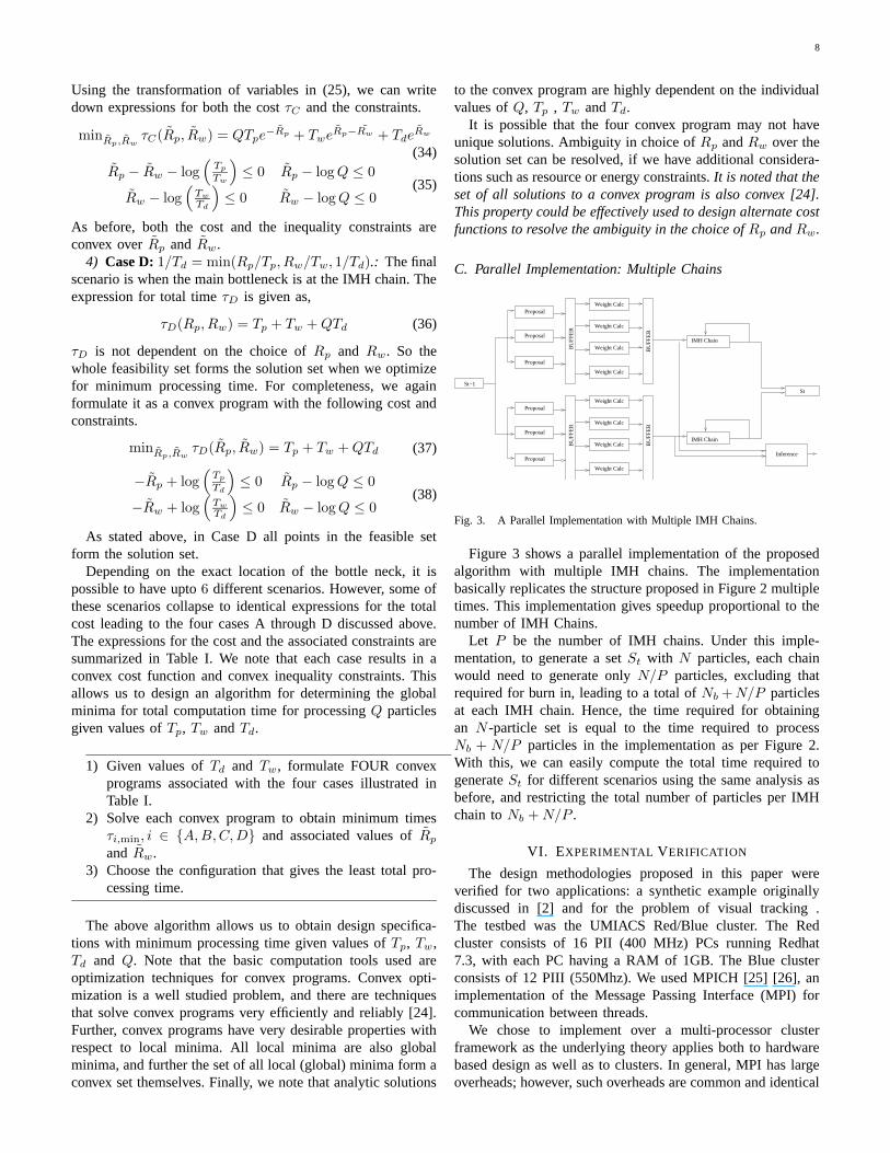
C. Parallel Implementation: Multiple Chains

St−1

Weight Calc

Weight Calc

Weight Calc

Weight Calc

Weight Calc

Weight Calc

Weight Calc

Weight Calc

BU

FFE

R

BU

FFE

R

Proposal

Proposal

Proposal

Proposal

BU

FFE

R

BU

FFE

R

Proposal

Proposal

IMH Chain

IMH Chain

Inference

St

Fig. 3. A Parallel Implementation with Multiple IMH Chains.

Figure 3 shows a parallel implementation of the proposedalgorithm with multiple IMH chains. The implementationbasically replicates the structure proposed in Figure 2 multipletimes. This implementation gives speedup proportional to thenumber of IMH Chains.

Let P be the number of IMH chains. Under this imple-mentation, to generate a set St with N particles, each chainwould need to generate only N/P particles, excluding thatrequired for burn in, leading to a total of Nb + N/P particlesat each IMH chain. Hence, the time required for obtainingan N -particle set is equal to the time required to processNb + N/P particles in the implementation as per Figure 2.With this, we can easily compute the total time required togenerate St for different scenarios using the same analysis asbefore, and restricting the total number of particles per IMHchain to Nb + N/P .

VI. EXPERIMENTAL VERIFICATION

The design methodologies proposed in this paper wereverified for two applications: a synthetic example originallydiscussed in [2] and for the problem of visual tracking .The testbed was the UMIACS Red/Blue cluster. The Redcluster consists of 16 PII (400 MHz) PCs running Redhat7.3, with each PC having a RAM of 1GB. The Blue clusterconsists of 12 PIII (550Mhz). We used MPICH [25] [26], animplementation of the Message Passing Interface (MPI) forcommunication between threads.

We chose to implement over a multi-processor clusterframework as the underlying theory applies both to hardwarebased design as well as to clusters. In general, MPI has largeoverheads; however, such overheads are common and identical

9

Case Rate Ordering Cost Constraint

A Rp/Tp ≤ Rw/Tw ≤ 1/Td QTpe−Rp + TweRp−Rw + TdeRwRp − Rw − log

(

Tp

Tw

)

≤ 0 Rp − log Q ≤ 0

Rw − log(

Tw

Td

)

≤ 0 Rw − log Q ≤ 0

B Rw/Tw = min(Rp/Tp, Rw/Tw, 1/Td) TpeRw−Rp + QTwe−Rw + TdeRwRw − Rp − log

(

Tw

Tp

)

≤ 0 Rp − log Q ≤ 0

Rw − log(

Tw

Td

)

≤ 0 Rw − Rp ≤ 0

C Rp/Tp ≤ 1/Td ≤ Rw/Tw QTpe−Rp + Tw + TdeRpRp − log

(

Tp

Td

)

≤ 0 Rp − log Q ≤ 0

−Rw + log(

Tw

Td

)

≤ 0 Rw − log Q ≤ 0

D 1/Td = min(Rp/Tp, Rw/Tw, 1/Td) Tp + Tw + QTd

−Rp + log(

Tp

Td

)

≤ 0 Rp − log Q ≤ 0

−Rw + log(

Tw

Td

)

≤ 0 Rw − log Q ≤ 0

TABLE IEXPRESSIONS FOR TOTAL TIME TAKEN TO PROCESS Q PARTICLES FOR BOTTLENECKS AT VARIOUS STAGES IN THE PIPELINE.

to both SISR as well as the MCMC based schemes. Theconclusions from our experimental observations still remainthe same.

Further, as mentioned earlier, computation of the burn-inperiod is a hard problem by itself. However, in sequentialestimation, the proposal density is in general a good guessof the posterior. In such cases, the adverse effects of burn-inperiod are reduced. For the experiments below, we set Nb = 0.

A. Visual Tracking

We implemented the particle filter based online trackingalgorithm presented in [27] using the Red Cluster. We discussthe finer details of the filter and its implementation below.

1) Model Details: We first summarize the tracking algo-rithm, detailing its computational aspects. A typical trackingexample in shown in Figure 4. The models defining thedynamical system is described below.

• State Space: The state xt is a 6-dimensional vector(X = R

6) defining affine deformations of a rectangulartemplate.

• State Transition Model: A simple random walk modelwith Gaussian noise is used to model the state transition.

xt = xt−1 + nt, nt ∼ N(0,Σn) (39)

• Observation Model: The frame of the video at timet forms the observation. The likelihood model p(yt|xt)involves comparing the appearance model At suitablydeformed by the state xt with the observation yt. Theappearance model employs a mixtures of Gaussians withthree mixtures to model the appearance. Each value of xt

defines a patch (parallelogram shaped) on the image yt.Let zt = T (yt;xt) be the patch defined by xt over yt.Then,

p(yt|xt) = p(yt|xtAt) = p(zt|At) (40)

• Proposal Density: The algorithm uses the proposal den-sity to be the same as the state transition model.

2) Implementation Details: An estimate of Tp, Tw and Td

was first obtained by running each block over a single PCmany times over and averaging the individual runs.

• Tp = 8µs, Tw = 1.1ms, Td = 1µs

With this, we can see that the main computational bottleneckfor this particular application is the evaluation of weights. Theweight computation has an unusually large latency, primarilybecause it involves retrieval from the memory. Given a particle,to compute the weight we need to first obtain the templatez(i)t = T (yt;x

(i)t ). This involves retrieval of elements from the

memory (containing the current frame). Further, the evaluationp(z

(i)t |At) involves evaluation of the mixture of Gaussian,

which is far more complicated than the simple proposal andthe IMHA blocks. For this reason, we fixed Rp = Rd = 1 andanalyzed the performance of the architecture for various valuesof Rw. The implementation of the proposed methodologyover the cluster was as follows. Each block (as shown infigure 3) was assigned a cluster node for itself, i.e, a total ofRp +Rw +Rd cluster nodes were employed, with Rp of themperforming particle proposal, Rw of them computing weightsand Rd, the IMH chains. Communication between these PCswas performed using MPICH libraries. Holding the values ofRp and Rw at unity (Rp = 1 = Rd), the tracker was testedfor varying number of weight computation blocks.

For comparison purposes, we also implemented traditionalSISR with the same specifications as the proposed methodol-ogy. The main difference was that the node that performedresampling would now wait till all particles are deliveredfrom the weight computation blocks before starting the SRalgorithm.

3) Results: The algorithm was used to process 20 framesof a video sequence, tracking a car. Figure 4 shows typicaltracking results. The filter was run with 840 and 1680 particles,with the number of cluster nodes for weight computation Rw

varying from 1 to 6. Rw = 1 corresponds to the sequentialimplementation, and Rw > 1 corresponds to the parallelimplementation with a single chain. Under the same setup,we tried an implementation of SISR, replacing the IMH Chainwith a systematic resampler. The main difference between thealgorithms is that the systematic resampler could begin onlywhen all particles were processed and the normalized weightsare known.

Figure 5(a) shows the actual time taken (in seconds) toprocess 20 frames of video, with 840/1680 particles for theproposed algorithm and SISR. Note the 1/x-like decay exhib-ited by the time taken by the proposed algorithm. Figure 5(b)

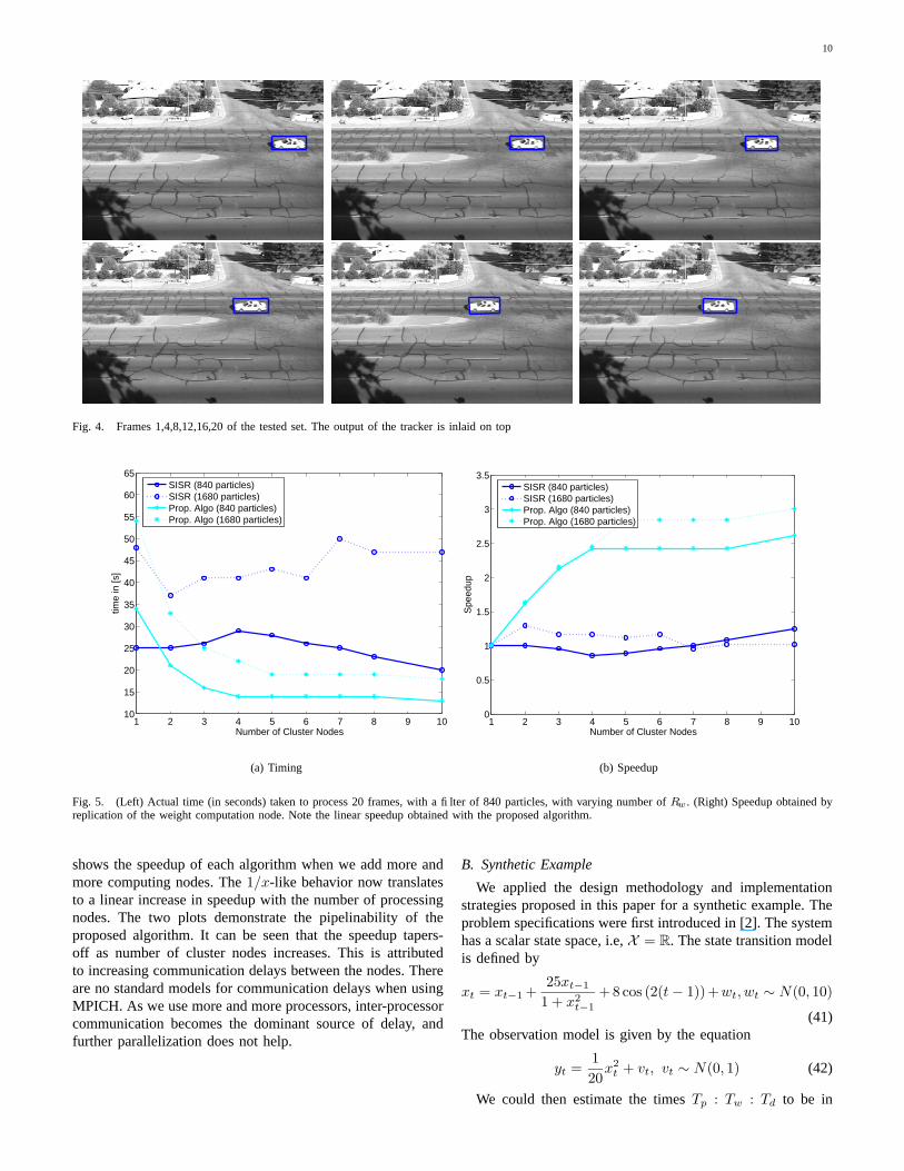
10

Fig. 4. Frames 1,4,8,12,16,20 of the tested set. The output of the tracker is inlaid on top

1 2 3 4 5 6 7 8 9 1010

15

20

25

30

35

40

45

50

55

60

65

Number of Cluster Nodes

time

in [s

]

SISR (840 particles)SISR (1680 particles)Prop. Algo (840 particles)Prop. Algo (1680 particles)

(a) Timing

1 2 3 4 5 6 7 8 9 100

0.5

1

1.5

2

2.5

3

3.5

Number of Cluster Nodes

Spe

edup

SISR (840 particles)SISR (1680 particles)Prop. Algo (840 particles)Prop. Algo (1680 particles)

(b) Speedup

Fig. 5. (Left) Actual time (in seconds) taken to process 20 frames, with a filter of 840 particles, with varying number of Rw . (Right) Speedup obtained byreplication of the weight computation node. Note the linear speedup obtained with the proposed algorithm.

shows the speedup of each algorithm when we add more andmore computing nodes. The 1/x-like behavior now translatesto a linear increase in speedup with the number of processingnodes. The two plots demonstrate the pipelinability of theproposed algorithm. It can be seen that the speedup tapers-off as number of cluster nodes increases. This is attributedto increasing communication delays between the nodes. Thereare no standard models for communication delays when usingMPICH. As we use more and more processors, inter-processorcommunication becomes the dominant source of delay, andfurther parallelization does not help.

B. Synthetic Example

We applied the design methodology and implementationstrategies proposed in this paper for a synthetic example. Theproblem specifications were first introduced in [2]. The systemhas a scalar state space, i.e, X = R. The state transition modelis defined by

xt = xt−1 +25xt−1

1 + x2t−1

+8 cos (2(t − 1))+wt, wt ∼ N(0, 10)

(41)The observation model is given by the equation

yt =1

20x2

t + vt, vt ∼ N(0, 1) (42)

We could then estimate the times Tp : Tw : Td to be in

11

the proportion 19.2 : 1 : 7. For filtering with Q = 840particles, we can now formulate and solve the four convexprograms. The convex programs were solved using the Mat-lab’s optimization toolbox. The constraints that are active (theconstraints that are satisfied with equality at a feasible pointare called active) at the minima were noted to give a qualitativeinterpretation to the result.

Case A: Minimum is achieved with the following two activeconstraints.

Rp

Tp

=Rw

Tw

=1

Td

(43)

Note that this is the rate balancing condition. The correspond-ing minimum time is

τA,min = QTd + Tp + Tw (44)

Case B: Again the minimum is achieved at the boundarywith the same active constraints.

Rw = RpRw

Tw= 1

Td

(45)

This gives us a minimum time of

τB,min = Tp + QTd + Tw (46)

Case C: Note that the cost function is independent of Rw.The minimum is achieved at the following active constraint.

Rp

Tp

=1

Td

(47)

giving a minimum time

τC,min = QTd + Tw + Tp (48)

Case D: The cost function is constant over the feasible set.Hence, the minimum time is

τD,min = Tp + Tw + QTd (49)

It turns out that all four convex program give the sameminimum time, and this also corresponds to the solution givenwhen the rates are balanced as in (43). This is interesting asbalanced rates have an intuitive appeal.

We implemented three filters and tested them on the Red andBlue clusters. The first two filters were those using SISR andIMH for resampling, with the proposal density, being sameas the state transition model. The third filter was based onauxiliary particles, with a complicated proposal density definedas follows:

g(xt, k|xt−1yt) ∝ g(xt|x(k)t−1yt)g(k)

g(k) = c,

g(·|xkt−1yt) ∼ N(±

√

20|yt| + x(k)t|t−1, 1),

where x(k)t|t−1,= x

(k)t−1 +

25x(k)t−1

1+(xk)t−1)

2+ 8 cos (2(t − 1))

(50)This particular proposal density samples the auxiliary state

randomly, and mixes the observation with the predicted stateto concentrate more particles near the posterior modes.

Figure 6 shows the actual time for computation and theachieved speedup with parallelization for the three filters,

tested on both clusters. We tested the algorithm for varying Rp

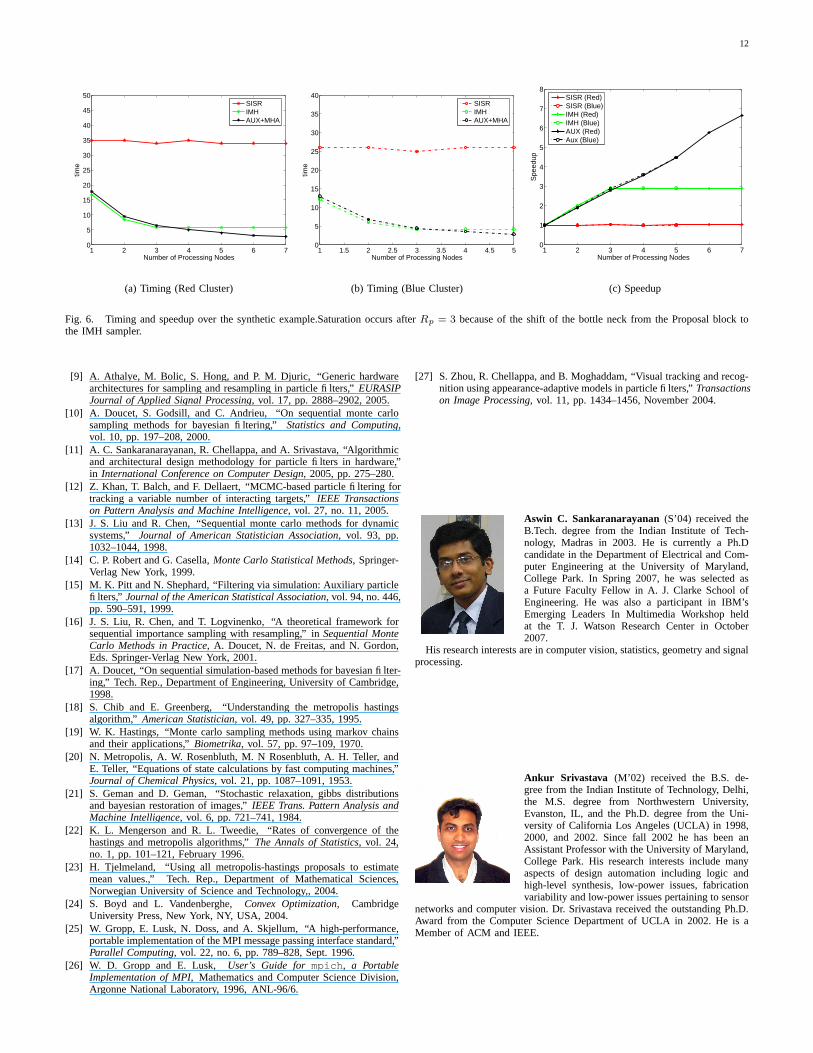
as the bottle-neck is initially in the proposal stage. Howeverfor Rp > Tp/Td ≈ 3 the bottleneck shifts to the IMH samplerand further increase in the value of Rp does not produceany significant gains in the overall processing time. This isreflected in the saturation of the plots associated with theproposed algorithm (IMH) in Figure 6. In contrast, in SISR theresampling begins only when all the particles are generated.The overall time for processing does not scale as well. Finally,auxiliary particle filtering scales linearly with the number ofprocessing nodes, and offers the best speedup.

The resampling method and the associated implementationschemes proposed in the paper, allows for a pipeline that is freeof bottle-necks. Further, implementations using the proposedmethodologies show a speedups that increases linearly withthe number of processing nodes utilized. This allows for us toparallelize the algorithm to achieve the desired runtime rate.In contrast, implementations based on SISR do not scale thateasily with the number of the processing nodes used.

VII. CONCLUSION

In this paper we address the computational challengesin implementing particle filters. We provide a methodologythat uses the Independent Metropolis Hastings sampler. Itis shown that the traditional bottleneck introduced by thesystematic resampler is removed. This allows for a bottle-neckfree pipelined implementation. The proposed algorithm worksindependent of the underlying application. Further, by usingthe auxiliary filter paradigm, we obtain an alternate design thatdoes not suffer (in complexity) in the presence of arbitraryproposal function. Finally, a set of convex programs is usedto compute the design specifications in terms of resourcesemployed in each stage of processing to achieve the minimumtime required to process a certain number of particles. Wevalidate our propositions using a cluster of PCs for the problemof visual tracking and show that implementations of theproposed methodology achieve speedup that is linear with thenumber of processing elements.

REFERENCES

[1] R. E. Kalman, “A new approach to linear filtering and predictionproblems,” Transactions of the ASME Journal of Basic Engineering,vol. 82, 1960.

[2] N. Gordon, D. Salmon, and A Smith, “Novel approach to nonlinear/non-gaussian bayesian state estimation,” Radar and Signal Processing, IEEProceedings F, vol. 140, pp. 107–113, 1993.

[3] A. Doucet, N. Freitas, and N. Gordon, Sequential Monte Carlo Methodsin Practice, Springer-Verlag New York, 2001.

[4] M. Isard and A. Blake, “Contour tracking by stochastic propagationof conditional density,” in European Conference on Computer Vision,1996, pp. 343–356.

[5] Q. Gang and R. Chellappa, “Structure from motion using sequentialmonte carlo methods,” International Journal of Computer Vision, vol.50(1), pp. 5–31, 2004.

[6] M. Bolic, P. M. Djuric, and S. Hong, “Resampling algorithms for particlefilters: A computational complexity perspective,” EURASIP Journal ofApplied Signal Processing, , no. 15, pp. 2267–2277, 2004.

[7] M. Bolic, P. M. Djuric, and S. Hong, “Resampling algorithms andarchitectures for distributed particle filters,” IEEE Transactions on SignalProcessing, vol. 53, no. 7, pp. 2442–2450, July 2005.

[8] M. Bolic, Architectures for Efficient Implementation of Particle Filters,Ph.D. thesis, Dept. of Electrical Engineering, State University of NewYork at Stony Brook, August 2004.

12

1 2 3 4 5 6 70

5

10

15

20

25

30

35

40

45

50

Number of Processing Nodes

time

SISRIMHAUX+MHA

(a) Timing (Red Cluster)

1 1.5 2 2.5 3 3.5 4 4.5 50

5

10

15

20

25

30

35

40

Number of Processing Nodes

time

SISRIMHAUX+MHA

(b) Timing (Blue Cluster)

1 2 3 4 5 6 70

1

2

3

4

5

6

7

8

Number of Processing Nodes

Spe

edup

SISR (Red)SISR (Blue)IMH (Red)IMH (Blue)AUX (Red)Aux (Blue)

(c) Speedup

Fig. 6. Timing and speedup over the synthetic example.Saturation occurs after Rp = 3 because of the shift of the bottle neck from the Proposal block tothe IMH sampler.

[9] A. Athalye, M. Bolic, S. Hong, and P. M. Djuric, “Generic hardwarearchitectures for sampling and resampling in particle filters,” EURASIPJournal of Applied Signal Processing, vol. 17, pp. 2888–2902, 2005.

[10] A. Doucet, S. Godsill, and C. Andrieu, “On sequential monte carlosampling methods for bayesian filtering,” Statistics and Computing,vol. 10, pp. 197–208, 2000.

[11] A. C. Sankaranarayanan, R. Chellappa, and A. Srivastava, “Algorithmicand architectural design methodology for particle filters in hardware,”in International Conference on Computer Design, 2005, pp. 275–280.

[12] Z. Khan, T. Balch, and F. Dellaert, “MCMC-based particle filtering fortracking a variable number of interacting targets,” IEEE Transactionson Pattern Analysis and Machine Intelligence, vol. 27, no. 11, 2005.

[13] J. S. Liu and R. Chen, “Sequential monte carlo methods for dynamicsystems,” Journal of American Statistician Association, vol. 93, pp.1032–1044, 1998.

[14] C. P. Robert and G. Casella, Monte Carlo Statistical Methods, Springer-Verlag New York, 1999.

[15] M. K. Pitt and N. Shephard, “Filtering via simulation: Auxiliary particlefilters,” Journal of the American Statistical Association, vol. 94, no. 446,pp. 590–591, 1999.

[16] J. S. Liu, R. Chen, and T. Logvinenko, “A theoretical framework forsequential importance sampling with resampling,” in Sequential MonteCarlo Methods in Practice, A. Doucet, N. de Freitas, and N. Gordon,Eds. Springer-Verlag New York, 2001.

[17] A. Doucet, “On sequential simulation-based methods for bayesian filter-ing,” Tech. Rep., Department of Engineering, University of Cambridge,1998.

[18] S. Chib and E. Greenberg, “Understanding the metropolis hastingsalgorithm,” American Statistician, vol. 49, pp. 327–335, 1995.

[19] W. K. Hastings, “Monte carlo sampling methods using markov chainsand their applications,” Biometrika, vol. 57, pp. 97–109, 1970.

[20] N. Metropolis, A. W. Rosenbluth, M. N Rosenbluth, A. H. Teller, andE. Teller, “Equations of state calculations by fast computing machines,”Journal of Chemical Physics, vol. 21, pp. 1087–1091, 1953.

[21] S. Geman and D. Geman, “Stochastic relaxation, gibbs distributionsand bayesian restoration of images,” IEEE Trans. Pattern Analysis andMachine Intelligence, vol. 6, pp. 721–741, 1984.

[22] K. L. Mengerson and R. L. Tweedie, “Rates of convergence of thehastings and metropolis algorithms,” The Annals of Statistics, vol. 24,no. 1, pp. 101–121, February 1996.

[23] H. Tjelmeland, “Using all metropolis-hastings proposals to estimatemean values.,” Tech. Rep., Department of Mathematical Sciences,Norwegian University of Science and Technology,, 2004.

[24] S. Boyd and L. Vandenberghe, Convex Optimization, CambridgeUniversity Press, New York, NY, USA, 2004.

[25] W. Gropp, E. Lusk, N. Doss, and A. Skjellum, “A high-performance,portable implementation of the MPI message passing interface standard,”Parallel Computing, vol. 22, no. 6, pp. 789–828, Sept. 1996.

[26] W. D. Gropp and E. Lusk, User’s Guide for mpich, a PortableImplementation of MPI, Mathematics and Computer Science Division,Argonne National Laboratory, 1996, ANL-96/6.

[27] S. Zhou, R. Chellappa, and B. Moghaddam, “Visual tracking and recog-nition using appearance-adaptive models in particle filters,” Transactionson Image Processing, vol. 11, pp. 1434–1456, November 2004.

Aswin C. Sankaranarayanan (S’04) received theB.Tech. degree from the Indian Institute of Tech-nology, Madras in 2003. He is currently a Ph.Dcandidate in the Department of Electrical and Com-puter Engineering at the University of Maryland,College Park. In Spring 2007, he was selected asa Future Faculty Fellow in A. J. Clarke School ofEngineering. He was also a participant in IBM’sEmerging Leaders In Multimedia Workshop heldat the T. J. Watson Research Center in October2007.

His research interests are in computer vision, statistics, geometry and signalprocessing.

Ankur Srivastava (M’02) received the B.S. de-gree from the Indian Institute of Technology, Delhi,the M.S. degree from Northwestern University,Evanston, IL, and the Ph.D. degree from the Uni-versity of California Los Angeles (UCLA) in 1998,2000, and 2002. Since fall 2002 he has been anAssistant Professor with the University of Maryland,College Park. His research interests include manyaspects of design automation including logic andhigh-level synthesis, low-power issues, fabricationvariability and low-power issues pertaining to sensor

networks and computer vision. Dr. Srivastava received the outstanding Ph.D.Award from the Computer Science Department of UCLA in 2002. He is aMember of ACM and IEEE.

13

Rama Chellappa (F’92) received the B.E. (Hons.)degree from the University of Madras, India, in 1975and the M.E. (Distinction) degree from the IndianInstitute of Science, Bangalore, in 1977. He receivedthe M.S.E.E. and Ph.D. Degrees in electrical engi-neering from Purdue University, West Lafayette, IN,in 1978 and 1981 respectively.

Since 1991, he has been a Professor of electricaland computer engineering and an affiliate Professorof computer science at the University of Maryland,College Park. He is also affiliated with the Center

for Automation Research (Director), the Institute for Advanced ComputerStudies (Permanent member), the Applied Mathematics program and theChemical Physics program. In 2005, he was named a Minta Martin Professorof Engineering. Prior to joining the University of Maryland, he was anAssistant (1981-1986) and Associate Professor (1986-1991) and Directorof the Signal and Image Processing Institute (1988-1990) at University ofSouthern California, Los Angeles. Over the last 26 years, he has publishednumerous book chapters and peer-reviewed journal and conference papers.He has also co-edited and co-authored many research monographs on Markovrandom fields, biometrics and surveillance. His current research interests arein face and gait analysis, 3-D modeling from video, automatic target recog-nition from stationary and moving platforms, surveillance and monitoring,hyperspectral processing, image understanding, and commercial applicationsof image processing and understanding.

Dr. Chellappa has served as an Associate Editor of four IEEE Transactions.He was a co-Editor-in-Chief of Graphical models and Image Processing.He also served as the Editor-in-Chief of the IEEE Transactions on PatternAnalysis and Machine Intelligence. He served as a member of the IEEE SignalProcessing Society Board of Governors and as its Vice President of Awardsand Membership. He has received several awards, including the NationalScience Foundation Presidential Young Investigator Award in 1985, three IBMFaculty Development Awards, the 1990 Excellence in Teaching Award fromthe School of Engineering at USC, the 1992 Best Industry Related PaperAward from the International Association of Pattern Recognition (with Q.Zheng), and the 2000 Technical Achievement Award from the IEEE SignalProcessing Society. He was elected as a Distinguished Faculty ResearchFellow (1996 to 1998), and as a Distinguished Scholar-Teacher (2003) atUniversity of Maryland. He co-authored a paper that received the Best StudentPaper in the Computer Vision Track at the International Association of PatternRecognition in 2006. He is a co-recipient of the 2007 Outstanding Innovatorof the Year Award (with A. Sundaresan) from the Office of TechnologyCommercialization at University of Maryland and received the 2007 A.J. ClarkSchool of Engineering Faculty Outstanding Research Award. He was recentlyelected to serve as a Distinguished Lecturer of the Signal Processing Societyand receive the Societys Meritorious Service Award. He is a Golden CoreMember of the IEEE Computer Society and received its Meritorious ServiceAward in 2004. He has served as a General and Technical Program Chair forseveral IEEE international and national conferences and workshops He is aFellow of the International Association for Pattern Recognition.