ALGORITHMIC RANDOMNESS AND FOURIER ANALYSIS

ALGORITHMIC RANDOMNESS AND FOURIER ANALYSIS

JOHANNA N.Y. FRANKLIN, TIMOTHY H. MCNICHOLL, AND JASON RUTE

Abstract. Suppose 1 < p < ∞. Carleson’s Theorem states that the Fourier

series of any function in Lp[−π, π] converges almost everywhere. We show

that the Schnorr random points are precisely those that satisfy this theoremfor every f ∈ Lp[−π, π] given natural computability conditions on f and p.

1. Introduction

Recent discoveries have shown that algorithmic randomness has a very naturalconnection with classical analysis. Many theorems in analysis have the form “Foralmost every x, . . .”; the set of points for which the central claim of the theoremfails for a given choice of parameters is called an exceptional set of the theorem. Forexample, one of Lebesgue’s differentiation theorems states that if f is a monotonefunction on [0, 1], then f is differentiable almost everywhere. In this case, for eachmonotone function f on [0, 1], the set of points at which f is not differentiableis an exceptional set. On the other hand, every natural randomness notion ischaracterized by a conull class of points. This suggests it is possible to characterizethe points that satisfy a particular theorem in analysis in terms of a randomnessnotion. Put another way, it may be the case that exceptional sets of a theorem canbe used to characterize a standard notion of randomness.

To date, results of this nature have been discovered in ergodic theory [4, 19, 20,22, 26, 36, 50], differentiability [5, 6, 21, 27, 36, 40, 43], Brownian motion [1, 2, 18],and other topics in analysis [3, 9, 45]. In this paper, we add Fourier series to thislist by considering Carleson’s Theorem. The original version of this theorem wasproven in 1966 by L. Carleson for L2 functions [10]; we will consider an extensionof this theorem to Lp functions for p > 1 that is due to Hunt but still generallyreferred to as Carleson’s Theorem [28]. Throughout this paper we only considerthe complex version of Lp[−π, π]; that is, we work in the space of all measurablef : [−π, π]→ C so that

∫ π−π |f(t)|p dt <∞.

Carleson’s Theorem. Suppose 1 < p <∞. If f is a function in Lp[−π, π], thenthe Fourier series of f converges to f almost everywhere.

Suppose 1 < p <∞. It is well known that the Fourier series of any f ∈ Lp[−π, π]converges to f in the Lp-norm. It follows that if the Fourier series of f ∈ Lp[−π, π]converges almost everywhere, then it converges to f almost everywhere.

We consider Carleson’s Theorem in the context of computable analysis anddemonstrate the points that satisfy this theorem are precisely the Schnorr randompoints via the following two theorems.

Theorem 1.1. Suppose p > 1 is a computable real. If t0 ∈ [−π, π] is Schnorrrandom and f is a computable vector in Lp[−π, π], then the Fourier series for fconverges at t0.

1

2 FRANKLIN, MCNICHOLL, AND RUTE

Theorem 1.2. If t0 ∈ [−π, π] is not Schnorr random, then there is a computablefunction f : [−π, π]→ C whose Fourier series diverges at t0.

It is well known that when p ≥ 1 is a computable real, there are incomputablefunctions in Lp[−π, π] that are nevertheless computable as vectors, e.g., step func-tions. Thus, Theorem 1.2 is considerably stronger than the converse of Theorem1.1. To the best of our knowledge, Theorems 1.1 and 1.2 yield the first characteri-zation of a randomness notion via a theorem of Fourier analysis. The proofs revealsome interesting and sometimes surprising connections between topics from algo-rithmic randomness such as Schnorr integral tests and topics from classical analysissuch as analytic and harmonic function theory.

The paper is organized as follows. In Section 2, we present the necessary back-ground. Sections 3 and 4 contain the proofs of Theorems 1.1 and 1.2, respectively.In Sections 5 and 6 we give two variations of Theorem 1.1. The first variation char-acterizes the values to which the Fourier series converges. The second variationaddresses the Fejer-Lebesgue Theorem which is similar to Carleson’s Theorem, butalso applies to the L1 case. Section 7 contains a broader analysis of our results.

2. Background and preliminaries

We begin with the necessary topics from analysis and then discuss computableanalysis and algorithmic randomness. We assume the reader is familiar with clas-sical computability in discrete settings as expounded in [12, 41, 42, 46].

2.1. Fourier analysis. We begin with some notation. For all n ∈ Z and t ∈[−π, π], let en(t) = eint. For all n ∈ Z and f ∈ L1[−π, π], let

cn(f) =1

2π

∫ π

−πf(t)eintdt.

For all f ∈ L1[−π, π] and all N ∈ N, let

SN (f) =

N∑n=−N

cn(f)en.

That is, SN (f) is the (N + 1)st partial sum of the Fourier series of f . We say thatf ∈ L1[−π, π] is analytic if cn(f) = 0 whenever n < 0.

C. Fefferman showed that when 1 < p <∞, there is a constant C so that

‖ supN|SN (f)|‖1 ≤ C‖f‖p

for all f ∈ Lp[−π, π] [15, 16]. We can (and do) assume that C is a positive integer.The operator f 7→ supN |SN (f)| is known as the Carleson operator.

Let E = {en : n ∈ Z}. A trigonometric polynomial is a function in the linearspan of E. If p is a trigonometric polynomial, then the degree of p is the smallestd ∈ N so that Sd(p) = p.

2.2. Complex analysis. We now summarize the required information on analyticand harmonic functions, in particular harmonic measure. This material will be usedexclusively in Section 4 (the proof of Theorem 1.2). More expansive treatments ofanalytic and harmonic functions can be found in [11] and [38]; the material onharmonic functions is drawn from [24].

ALGORITHMIC RANDOMNESS AND FOURIER ANALYSIS 3

Suppose U ⊆ C is open and connected. Recall that a function f : U → C isanalytic if it has a power series expansion at each point of U ; equivalently, if f isdifferentiable at each z0 ∈ U in the sense that

limz→z0

f(z)− f(z0)

z − z0exists.

Let D denote the unit disk, and let λ denote Lebesgue measure on the unit circle.The points on the unit circle are called the unimodular points. When f is analyticon D, let

an(f) =f (n)(0)

n!

for all n ∈ N. That is, an(f) is the (n+ 1)st coefficient of the MacLaurin series off . Thus,

f(z) =

∞∑n=0

an(f)zn

for all z ∈ D.Now we turn our attention to harmonic functions. Again, let U be a subset of

the plane that is open and connected. Recall that a function u : U → R is harmonicif it is twice continuously differentiable and satisfies Laplace’s equation

∂2u

∂x2+∂2u

∂y2= 0.

When u is harmonic on D, let u denote the harmonic conjugate of u that maps 0to 0. That is, u is the harmonic function on D so that u(0) = 0 and so that u andu satisfy the Cauchy-Riemann equations:

∂u

∂x=∂u

∂y

∂u

∂y= −∂u

∂x.

Let u = u+ iu. Thus, u is analytic and is called the analytic extension of u.When B is a Borel subset of the unit circle, there is a harmonic function u on

the unit disk so that for all unimodular ζ, limz→ζ u(z) = χB(ζ) (where χA denotesthe characteristic function of A); let ω(z,B,D) = u(z). The quantity ω(z,B,D) iscalled the harmonic measure of B at z. For each z in the unit disk, ω(z, ·,D) is aBorel probability measure on the unit circle. Moreover, ω(0, B,D) = (2π)−1λ(B)[24].

An explicit formula for the harmonic measure of an open arc on the unit circlecan be obtained as follows. Let Log denote the principal branch of the complexlogarithm. That is,

Log(z) =

∫ z

1

1

ζdζ

for all points z that do not lie on the negative real axis. Let Arg = Im(Log).Suppose A = {eiθ : θ1 < θ < θ2} where −π < θ1 < θ2 < π. Then

ω(z,A,D) =1

πArg

(z − eiθ2z − eiθ1

)− 1

2π(θ2 − θ1).


(See Exercise 1 on p. 26 of [24].) It follows that

ω(z,A,D) =1

πln

∣∣∣∣z − eiθ2z − eiθ1

∣∣∣∣ and(2.1)

ω(z,A,D) =1

πiLog

(z − eiθ2z − eiθ1

)− 1

2π(θ2 − θ1).(2.2)

2.3. Computable analysis. We now use the classical concepts of computabilityin a discrete setting to define the concept of computability in a continuous setting.

A complex number z is computable if there is an algorithm that, given a non-negative integer k as input, computes a rational point q so that |q − z| < 2−k.A sequence {an}n∈Z of points in the plane is computable if there is an algorithmthat, given an n ∈ Z and a k ∈ N as input, computes a rational point q so that|an − q| < 2−k.

Let us call a trigonometric polynomial τ rational if each of its coefficients is arational point.

Definition 2.1. Suppose p ≥ 1 is a computable real and suppose f ∈ Lp[−π, π].Then f is a computable vector of Lp[−π, π] if there is an algorithm that, given k ∈ Nas input, computes a rational polynomial τ so that ‖f − τ‖p < 2−k.

In other words, a vector f ∈ Lp[−π, π] is computable if it is possible to computearbitrarily good approximations of f by rational trigonometric polynomials.

The next proposition states the fundamental computability results we shall needabout vectors in Lp[−π, π].

Proposition 2.2. Suppose p ≥ 1 is a computable real and f ∈ Lp[−π, π].

(1) If f is a computable vector, then ‖f‖p and {cn(f)}n∈Z are computable.(2) If p = 2, then f is computable if both ‖f‖2 and {cn(f)}n∈Z are computable.

Proof. Suppose τ is a rational trigonometric polynomial. The Lp-norm of τ can becomputed directly from τ . Since |‖f‖p − ‖τ‖p| ≤ ‖f − τ‖p, it follows that ‖f‖p iscomputable. We also have

|cn(f)− cn(τ)|p =

∣∣∣∣∫ π

−π(f(θ)− τ(θ))einθ

dθ

2π

∣∣∣∣p≤(∫ π

−π|f(θ)− τ(θ)| dθ

2π

)p≤∫ π

−π|f(θ)− τ(θ)|p dθ

2π= ‖f − τ‖pp,

where the last step is by Jensen’s Inequality. It follows that {cn(f)}n∈Z is com-putable.

Now suppose p = 2 and suppose {cn(f)}n∈Z and ‖f‖2 are computable. Since‖f‖22 =

∑n∈Z |cn(f)|2 and ‖f − SN (f)‖22 =

∑|n|>N |cn(f)|2, it follows that f is a

computable vector in L2[−π, π]. �

The following corollary shows that the computability of a vector in Lp[−π, π] isdistinct from the computability of its Fourier coefficients.

Corollary 2.3. There is an incomputable vector f ∈ L2[−π, π] so that {cn(f))}n∈Zis computable.


Proof. Let {rn}n∈N be any computable sequence of positive rational numbers sothat

∑∞n=0 r

2n is incomputable. (The existence of such a sequence follows from the

constructions of E. Specker [48].) Set f =∑∞n=0 rnen. Then ‖f‖22 =

∑∞n=0 r

2n is

incomputable. Thus, by Proposition 2.2, f is incomputable. �

We now discuss computability of planar sets and functions. A comprehensivetreatment of the computability of functions and sets in continuous settings canbe found in [51]; the reader may also see [49], [25], [32], [33], [7], [44], and [8]. Tobegin, an interval is rational if its endpoints are rational numbers. An open (closed)rational rectangle is a Cartesian product of open (closed) rational intervals.

An open subset of the plane U is computably open if it is open and the set ofall closed rational rectangles that are included in U is computably enumerable. Onthe other hand, an open subset of the real line X is computably open if the set ofall closed rational intervals that are included in X is computably open. A sequenceof open sets of reals {Un}n∈N is computable if Un is computably open uniformlyin n; that is, if there is an algorithm that, given any n ∈ N as input, produces analgorithm that enumerates the closed rational intervals included in Un.

Suppose X is a compact subset of the plane. A minimal cover of X is a finitesequence of open rational rectangles (R0, . . . , Rm) so that X ⊆

⋃j Rj and so that

X ∩ Rj 6= ∅ for all j ≤ m. We say that X is computably compact if the set of allminimal covers of X is computably enumerable.

Suppose f is a function that maps complex numbers to complex numbers. Wesay that f is computable if there is an algorithm P that satisfies the following threecriteria.

• Approximation: Whenever P is given an open rational rectangle as input,it either does not halt or produces an open rational rectangle as output.(Here, the input rectangle is regarded as an approximation of some z ∈dom(f) and the output rectangle is regarded as an approximation of f(z).)

• Correctness: Whenever P halts on an open rational rectangle R, the rec-tangle it outputs contains f(z) for each z ∈ R ∩ dom(f).

• Convergence: Suppose U is a neighborhood of a point z ∈ dom(f) andthat V is a neighborhood of f(z). Then, there is an open rational rectangleR such that R contains z, R is included in U , and when R is put into P ,P produces a rational rectangle that is included in V .

For example, sin, cos, and exp are computable as can be seen by considering theirpower series expansions and the bounds on the convergence of these series thatcan be obtained from Taylor’s Theorem. A consequence of this definition is thatcomputable functions on the complex plane must be continuous.

A sequence of functions {fn}n∈N of a complex variable is computable if it iscomputable uniformly in n; that is, there is an algorithm that given any n ∈ N asinput produces an algorithm that computes fn.

It is well known that integration is a computable functional on C[0, 1]. It fol-lows that when f is a computable analytic function on the unit disk, the sequence{an(f)}n∈N is computable uniformly in f . It also follows that Log is computable.

A modulus of convergence for a sequence {an}n∈N of points in a complete metricspace (X, d) is a function g : N→ N so that d(am, an) < 2−k whenever m,n ≥ g(k).Thus, a sequence of points in a complete metric space converges if and only if it has amodulus of convergence. Suppose p ≥ 1 is computable. If {fn}n∈N is a computable


and convergent sequence of vectors in Lp[−π, π], then limn fn is a computable vectorif and only if {fn}n∈N has a computable modulus of convergence.

Suppose f is a uniformly continuous computable function that maps complexnumbers to complex numbers. A modulus of uniform continuity for f is a functionm : N→ N so that |f(z0)− f(z1)| < 2−k whenever z0, z1 ∈ dom(f) and |z0 − z1| ≤2−m(k). If the domain of f is computably compact, then f has a computablemodulus of uniform continuity.

Suppose {an}n∈N is a sequence of complex numbers so that∑∞n=0 anz

n convergeswhenever |z| < 1, and suppose G is a compact subset of the unit disk. A modulusof uniform convergence for this series on G is a function m : N → N so that∣∣∣∑∞n=m(k) anz

n∣∣∣ < 2−k whenever z ∈ G and k ∈ N. If the sequence {an}n∈N is

computable and if G is computably compact, then the series∑∞n=0 anz

n has acomputable modulus of uniform convergence on G.

We note that when p ≥ 1 is a computable real and f ∈ Lp[−π, π], there are twosenses in which f can be “computable”: as a vector and as a function. These failto coincide. By definition, a computable function is continuous. However, thereare discontinuous functions in L1[−π, π] that are computable as vectors; e.g., thegreatest integer function. Moreover, there are continuous functions in L1[−π, π]that are computable as vectors but not as functions.

Lastly, a lower semicomputable function is a function T : [−π, π] → [0,∞] thatis the sum of a computable sequence of nonnegative real-valued functions.

2.4. Algorithmic randomness. There are three different approaches to definingthe concept of randomness formally. The one we will find useful for this paper isthe measure-theoretic one: A random point in a given probability space is said tobe random if it avoids all null classes generated in a certain way by computablyenumerable functions. Thus, for any reasonable randomness notion, the class ofrandom points is conull. For a general introduction to algorithmic randomness, see[14] or [39].

While the most-studied randomness notion is Martin-Lof randomness, a weakernotion, Schnorr randomness, lies at the heart of our paper. Schnorr randomness,like most other randomness notions, was originally defined in the Cantor space2ω with Lebesgue measure [47]; however, the definition is easily adaptable to anycomputable measure space, in particular [−π, π] with the Lebesgue measure µ.

Definition 2.4. A Schnorr test is a computable sequence {Vn}n∈N of open setsof reals so that µ(Vn) ≤ 2−n for all n and so that the sequence {µ(Vn)}n∈N iscomputable. A real number x is said to be Schnorr random if for every Schnorrtest {Vn}n∈N, x 6∈

⋂n Vn.

There are many other characterizations of Schnorr randomness, such as a complexity-based characterization [13] and a martingale characterization [47]. In this paper,we will use an integral test characterization due to Miyabe [35] which is rooted incomputable analysis.

Definition 2.5. A Schnorr integral test is a lower semicomputable function T :[−π, π]→ [0,∞] so that

∫ π−π T dµ is a computable real.

Thus, if T is a Schnorr integral test, then T (x) is finite for almost every x ∈[−π, π]. Miyabe’s characterization states that x ∈ [−π, π] is Schnorr random if andonly if T (x) <∞ for every Schnorr integral test T .


3. Proof of Theorem 1.1

Our proof of Theorem 1.1 is based on the following definition and lemmas.

Definition 3.1. Suppose {fn}n∈N is a sequence of functions on [−π, π]. A functionη : N× N→ N is a modulus of almost-everywhere convergence for {fn}n∈N if

µ({t ∈ [−π, π] : ∃M,N ≥ η(k,m) |fN (t)− fM (t)| ≥ 2−k}) < 2−m

for all k and m.

Thus, every sequence of functions on [−π, π] that converges almost everywherehas a modulus of almost-everywhere convergence. Our goal, as stated in the fol-lowing lemma, is to show that the sequence of partial sums for the Fourier series ofa computable vector in Lp[−π, π] has a computable modulus of almost-everywhereconvergence.

Lemma 3.2. Suppose p is a computable real so that p > 1, and suppose f is acomputable vector in Lp[−π, π]. Then, {SN (f)}N∈N has a computable modulus ofalmost-everywhere convergence.

With this lemma in hand, Theorem 1.1 follows from the next lemma.

Lemma 3.3. Assume {fn}n∈N is a uniformly computable sequence of functions on[−π, π] for which there is a computable modulus of almost-everywhere convergence.Then, the sequence {fn}n∈N converges at every Schnorr random real.

Generalizations of Lemma 3.3 can be found in Galatolo, Hoyrup, and Rojas [23,Thm. 1] and well as Rute [45, Lemma 3.19 on p. 41]. Our proof is new. Theorem1.1 follows by applying Lemma 3.3 to the sequence of partial sums of f .

Proof of Lemma 3.2. We compute η : N2 → N as follows. Let k,m ∈ N be givenas input. Compute a rational trigonometric polynomial τk,m so that ‖f − τk,m‖p ≤2−(m+k+3)C−1 where C is as in Fefferman’s inequality. Then define η(k,m) to bethe degree of τk,m.

By definition, η is computable. We now show that it is a modulus of almost-everywhere convergence. We begin with some notation. Let g ∈ Lp[−π, π]. Set

Ek,N0(g) = {t ∈ [−π, π] : ∃M,N ≥ N0 |SM (g)(t)− SN (g)(t)| ≥ 2−k}.

Thus, we aim to show that µ(Ek,η(k,m)(f)) < 2−m. For each k ∈ N, let

Ek(g) = {t ∈ [−π, π] : supN|SN (g)(t)| > 2−k}.

It follows that Ek,N0(g) ⊆ Ek+2(g).

We claim that Ek,η(k,m)(f) ⊆ Ek,η(k,m)(f−τk,m). We see that if M,N ≥ η(k,m),then

|SM (f)(t)− SN (f)(t)| ≤ |SM (f − τk,m)(t)− SN (f − τk,m)(t)|+ |SM (τk,m)(t)− SN (τk,m)(t)|= |SM (f − τk,m)(t)− SN (f − τk,m)(t)|.

Thus, Ek,η(k,m)(f) ⊆ Ek,η(k,m)(f − τk,m).

It now follows that Ek,η(k,m)(f) ⊆ Ek+2(f − τk,m). We complete the proof

by showing that µ(Ek+2(f − τk,m)) < 2−m. By Fefferman’s Inequality and thedefinition of τk,m,

‖ supN|SN (f − τk,m)|‖1 ≤ 2−(m+k+3).


Thus, by Chebyshev’s Inequality,

µ(Ek+2(f − τk,m)) ≤ 2−(m+k+3)2k+2 = 2−(m+1) < 2−m.

Hence, µ(Ek+2(f − τk,m)) < 2−m. �

Proof of Lemma 3.3. We apply Miyabe’s characterization of Schnorr randomness.We begin by defining a Schnorr integral test as follows. Let η be a computablemodulus of almost-everywhere convergence for {fn}n∈N, and abbreviate η(k, k) byNk. For each k ∈ N and each t ∈ [−π, π] define

gk(t) = min {1, max{|fM (t)− fN (t))| : Nk < M,N ≤ Nk+1}} .The sequence {gk}k∈N is computable. Set T =

∑∞k=0 gk.

We now show that T is a Schnorr integral test. By construction, T is lowersemicomputable. Therefore, it suffices to show that

∫ π−π Tdµ is a computable real.

To this end, let m ∈ N be given. Since gk is computable uniformly in k, it is possibleto compute a rational number q so that |

∑m+6k=0 gk − q| < 2−(m+1). We claim that

|∫ π−π Tdµ− q| < 2−m. By the Monotone Convergence Theorem,∫ π

−πT dµ =

∞∑k=0

∫ π

−πgk dµ.

Since gk ≤ 1 and µ{t : gk(t) ≥ 2−k} ≤ 2−k, we have∫ π

−πgk(t) dt ≤ 2−k · µ{t : g(t) < 2−k}+ 1 · µ{t : g(t) ≥ 2−k}

≤ 2−k · 2π + 1 · 2−k ≤ 2−k+4.

Thus,∫ π−π T dµ −

∑m+6k=0 gk < 2−(m+1), and we then have |

∫ π−π T dµ − q| < 2−m.

Hence,∫ π−π T dµ is a computable real.

Finally, we show that T (t0) = ∞ whenever {fn(t0)}n∈N diverges. This willcomplete the proof of the lemma. Suppose {fn(t0)}n∈N diverges. Then there existsk0 ∈ N so that lim supM,N |fM (t0) − fN (t0)| ≥ 2−k0 . It thus suffices to show that∑∞k=k1

gk(t0) ≥ 2−k0 for all k1 ∈ N. So, let k1 ∈ N. Without loss of generality,suppose gk < 1 whenever k ≥ k1. By the choice of k0, there exist M and N so thatNk1 ≤ M < N and |fM (t0) − fN (t0)| ≥ 2−k0 . By forming a telescoping sum andapplying the triangle inequality we obtain

|fM (t0)− fN (t0)| ≤∞∑

k=k1

gk(t0).

Thus T (t0) =∞, and the proof is complete. �

4. Proof of Theorem 1.2

Our proof of Theorem 1.2 is based on a construction of Kahane and Katznelson[29] and requires the following sequence of three lemmas.

Lemma 4.1. Suppose G is a computably compact subset of the unit circle so thatλ(G) is computable and smaller than 2π. Then there is a computable function ψfrom D∪G into the horizontal strip R× (−π2 ,

π2 ) that is analytic on D and has the

property that Re(ψ(ζ)) ≥ − 34 ln(λ(G)(2π)−1) for all ζ ∈ G. Furthermore, we may

choose ψ so that ψ(0) = 0.


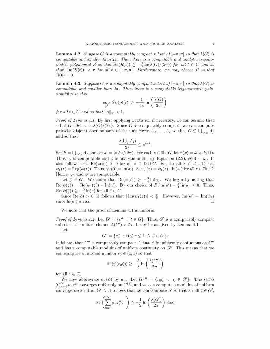
Lemma 4.2. Suppose G is a computably compact subset of [−π, π] so that λ(G) iscomputable and smaller than 2π. Then there is a computable and analytic trigono-metric polynomial R so that Re(R(t)) ≥ − 1

2 ln(λ(G)/(2π)) for all t ∈ G and sothat | Im(R(t))| < π for all t ∈ [−π, π]. Furthermore, we may choose R so thatR(0) = 0.

Lemma 4.3. Suppose G is a computably compact subset of [−π, π] so that λ(G) iscomputable and smaller than 2π. Then there is a computable trigonometric poly-nomial p so that

supN|SN (p)(t)| ≥ − 1

4πln

(λ(G)

2π

)for all t ∈ G and so that ‖p‖∞ < 1.

Proof of Lemma 4.1. By first applying a rotation if necessary, we can assume that−1 6∈ G. Set a = λ(G)/(2π). Since G is computably compact, we can computepairwise disjoint open subarcs of the unit circle A0, . . . , As so that G ⊆

⋃j≤sAj

and so thatλ(⋃j Aj)

2π≤ a3/4.

Set F =⋃j≤sAj and set a′ = λ(F )/(2π). For each z ∈ D∪G, let φ(x) = ω(z, F,D).

Thus, φ is computable and φ is analytic in D. By Equation (2.2), φ(0) = a′. Italso follows that Re(φ(z)) > 0 for all z ∈ D ∪ G. So, for all z ∈ D ∪ G, setψ1(z) = Log(φ(z)). Thus, ψ1(0) = ln(a′). Set ψ(z) = ψ1(z)−ln(a′) for all z ∈ D∪G.Hence, ψ1 and ψ are computable.

Let ζ ∈ G. We claim that Re(ψ(ζ)) ≥ − 34 ln(a). We begin by noting that

Re(ψ(ζ)) = Re(ψ1(ζ)) − ln(a′). By our choice of F , ln(a′) − 34 ln(a) ≤ 0. Thus,

Re(ψ(ζ)) ≥ − 34 ln(a) for all ζ ∈ G.

Since Re(φ) > 0, it follows that | Im(ψ1(z))| < π2 . However, Im(ψ) = Im(ψ1)

since ln(a′) is real. �

We note that the proof of Lemma 4.1 is uniform.

Proof of Lemma 4.2. Let G′ = {eit : t ∈ G}. Thus, G′ is a computably compactsubset of the unit circle and λ(G′) < 2π. Let ψ be as given by Lemma 4.1.

Let

G′′ = {rζ : 0 ≤ r ≤ 1 ∧ ζ ∈ G′}.It follows that G′′ is computably compact. Thus, ψ is uniformly continuous on G′′

and has a computable modulus of uniform continuity on G′′. This means that wecan compute a rational number r0 ∈ (0, 1) so that

Re(ψ(r0ζ)) ≥ −5

8ln

(λ(G′)

2π

)for all ζ ∈ G.

We now abbreviate an(ψ) by an. Let G(3) = {r0ζ : ζ ∈ G′}. The series∑∞n=0 anz

n converges uniformly on G(3), and we can compute a modulus of uniform

convergence for it on G(3). It follows that we can compute N so that for all ζ ∈ G′,

Re

(N∑n=0

anrn0 ζ

n

)≥ −1

2ln

(λ(G′)

2π

)and

10 FRANKLIN, MCNICHOLL, AND RUTE∣∣∣∣∣Im(

N∑n=0

anrn0 ζ

n

)∣∣∣∣∣ < π.

Set R(t) =∑Nn=0 anr

n0 eint. �

We note that the proof of Lemma 4.2 is also uniform.

Proof of Lemma 4.3. Let R be as given in Lemma 4.2 and let N = deg(R). Setq = Im(R) and p = 1

π e−N · q.We claim that |SN (p)| = 1

2π |R|. For convenience, we abbreviate cn(R) by cn.Then cm = 0 when m ≤ 0 and

q(t) =1

2i

[N∑n=1

cneint +

N∑n=1

(−cn)e−int

]and

p(t) =1

2πi

[0∑

m=1−Ncm+Ne

int +

2N∑m=1+N

(−cm−N )e−int

].

Therefore,

SN (p)(t) = e−iNt1

2πSN (R)(t).

Thus, |SN (p)| = 12π |R|.

Therefore,

supN|SN (p)(t)| ≥ − 1

4πln

(µ(G)

2π

)for all t ∈ G.

Since | Im(R)| < π, it follows that ‖p‖∞ < 1. �

Note that the proof of Lemma 4.3 is uniform as well.Now suppose t0 is not Schnorr random. Then there is a Schnorr test {Un}n∈N

so that t0 ∈⋂n Un.

We construct an array of trigonometric polynomials {pn,k}n,k∈N as follows. SinceU2n is computably open uniformly in N , we can compute an array of closed rationalintervals {In,j}n,j∈N so that U2n =

⋃j In,j and so that µ(In,j ∩ In,j′) = 0 when

j 6= j′. We then compute for each n ∈ N an increasing sequence mn,0 < mn,1 < . . .so that

µ

U2n −⋃

j≤mn,k

In,j

< 2−(2n+k+1)

for all n and k. We define the following sets:

Gn,0 =⋃

j≤mn,0

In,j ∩ [−π, π] and

Gn,k =⋃

mn,k<j≤mn,k+1

In,j ∩ [−π, π].

It follows that

µ(Gn,k) < 2−(2n+k)

for all n and k.


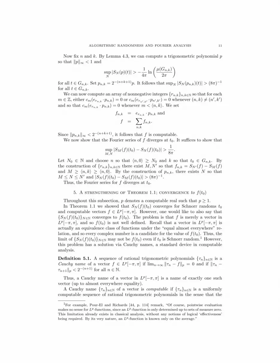
Now fix n and k. By Lemma 4.3, we can compute a trigonometric polynomial pso that ‖p‖∞ < 1 and

supN|SN (p)(t)| > − 1

4πln

(µ(Gn,k)

2π

)for all t ∈ Gn,k. Set pn,k = 2−(n+k+1)p. It follows that supN |SN (pn,k)(t)| > (8π)−1

for all t ∈ Gn,k.We can now compute an array of nonnegative integers {rn,k}n,k∈N so that for each

m ∈ Z, either cm(ern,k·pn,k) = 0 or cm(ern′,k′ ·pn′,k′) = 0 whenever (n, k) 6= (n′, k′)

and so that cm(ern,k· pn,k) = 0 whenever m < 〈n, k〉. We set

fn,k = ern,k· pn,k and

f =∑n,k

fn,k.

Since ‖pn,k‖∞ < 2−(n+k+1), it follows that f is computable.We now show that the Fourier series of f diverges at t0. It suffices to show that

supM,N|SM (f)(t0)− SN (f)(t0)| > 1

8π.

Let N0 ∈ N and choose n so that 〈n, 0〉 ≥ N0 and k so that t0 ∈ Gn,k. Bythe construction of {rn,k}n,k∈N there exist M,N ′ so that fn,k = SN ′(f) − SM (f)and M ≥ 〈n, k〉 ≥ 〈n, 0〉. By the construction of pn,k, there exists N so thatM ≤ N ≤ N ′ and |SN (f)(t0)− SM (f)(t0)| > (8π)−1.

Thus, the Fourier series for f diverges at t0.

5. A strengthening of Theorem 1.1; convergence to f(t0)

Throughout this subsection, p denotes a computable real such that p ≥ 1.In Theorem 1.1 we showed that SN (f)(t0) converges for Schnorr randoms t0

and computable vectors f ∈ Lp[−π, π]. However, one would like to also say that{SN (f)(t0)}N∈N converges to f(t0). The problem is that f is merely a vector inLp[−π, π], and so f(t0) is not well defined. Recall that a vector in Lp[−π, π] isactually an equivalence class of functions under the “equal almost everywhere” re-lation, and so every complex number is a candidate for the value of f(t0). Thus, thelimit of {SN (f)(t0)}N∈N may not be f(t0) even if t0 is Schnorr random.1 However,this problem has a solution via Cauchy names, a standard device in computableanalysis.

Definition 5.1. A sequence of rational trigonometric polynomials {τn}n∈N is aCauchy name of a vector f ∈ Lp[−π, π] if limn→∞ ‖τn − f‖p = 0 and if ‖τn −τn+1‖p < 2−(n+1) for all n ∈ N.

Thus, a Cauchy name of a vector in Lp[−π, π] is a name of exactly one suchvector (up to almost everywhere equality).

A Cauchy name {τn}n∈N of a vector is computable if {τn}n∈N is a uniformlycomputable sequence of rational trigonometric polynomials in the sense that the

1For example, Pour-El and Richards [44, p. 114] remark, “Of course, pointwise evaluation

makes no sense for Lp-functions, since an Lp-function is only determined up to sets of measure zero.This limitation already exists in classical analysis, without any notions of logical ‘effectiveness’

being required. By its very nature, an Lp-function is known only on the average.”


degree and coefficients of τn can be computed from n. It follows that a vector inLp[−π, π] is computable if and only if it has a computable Cauchy name.

We will show that there is a natural way to use a computable Cauchy name off ∈ Lp[−π, π] to assign a canonical value to f(t0) when t0 is Schnorr random. Wewill then show that if f is a computable vector in Lp[−π, π], then limN→∞ SN (f)(t0)is the canonical value of f(t0) whenever t0 is Schnorr random. Our approach isbased on the following theorem which effectivizes a well-known result in measuretheory; namely, that a convergent sequence in Lp[−π, π] has a subsequence thatconverges almost everywhere.

Theorem 5.2. Suppose fn ∈ Lp[−π, π] for all n ∈ N and suppose g is a computablemodulus of convergence for {fn}n∈N. Then, η(k,m) = d 12 (m+1

p + k + 1)e defines a

modulus of almost-everywhere convergence for {fg(2n)}n∈N.

Proof. Set

En,r = {t ∈ [−π, π] : |fg(2n+1)(t)− fg(2n)(t)| ≥ 2−r}.

Since g is a modulus of convergence for {fn}n∈N, ‖fg(2n+1) − fg(2n)‖pp < 2−2np.

Thus, by Chebychev’s Inequality, µ(En,r) ≤ 2p(r−2n).Set N0 = η(k,m). Suppose M,N ≥ N0 and |fg(2M)(t)− fg(2N)(t)| ≥ 2−k. Then

2−k ≤∞∑

n=N0

|fg(2m)(t)− fg(2n)(t)|.

It follows that t ∈⋃∞c=0EN0+c,k+1+c. But, by the definition of η,

∞∑c=0

2p(k+1+c−2(N0+c) <

∞∑c=m+1

2−c = 2−m.

Thus, µ(⋃∞c=0EN0+c,k+1+c) < 2−m. It follows that η is a modulus of almost-

everywhere convergence for {fg(2n)}n∈N. �

Corollary 5.3. If {τn}n∈N is a computable Cauchy name for a vector in Lp[−π, π]and if t0 ∈ [−π, π] is Schnorr random, then {τ2n(t0)}n∈N converges.

Corollary 5.3 leads to the idea that a Cauchy name for f assigns a value to f(t)for Schnorr random t.

Definition 5.4. If {τn}n∈N is a computable Cauchy name for a vector f ∈ Lp[−π, π],and if {τ2n(t)}n∈N converges to α ∈ C, then we say {τn}n∈N assigns the value α tof(t).

Thus, if f is a computable vector in Lp[−π, π] and if t0 is Schnorr random, thena value is assigned to f(t0) by each computable Cauchy name of f . We now showthat the same value is assigned by all computable Cauchy names via the followingproposition.

Proposition 5.5. Suppose {fn}n∈N and {gn}n∈N are computable sequence of func-tions on [−π, π] and that each has a computable modulus of almost-everywhere con-vergence. Suppose also that limn→∞ fn(t)− gn(t) = 0 for almost every t ∈ [−π, π].Then, limn→∞ fn(t0) = limn→∞ gn(t0) whenever t0 ∈ [−π, π] is Schnorr random.


Proof. Let η0 be a computable modulus of almost-everywhere convergence for{fn}n∈N, and let η1 be a computable modulus of almost-everywhere convergencefor {gn}n∈N. Let h2n = fn, and let h2n+1 = gn. Set η(k,m) = η0(k + 1,m + 2) +η1(k + 1,m + 2). It follows that η is a computable modulus of almost-everywhereconvergence for {hn}n∈N. So, if t0 is Schnorr random, then {hn(t0)}n∈N converges,and so {fn(t0)}n∈N and {gn(t0)}n∈N converge to the same value. �

Definition 5.6. Suppose f is a computable vector in Lp[−π, π]. When t0 is Schnorrrandom, the canonical value of f(t0) is the value assigned to f(t0) by a computableCauchy name of f .

By Proposition 5.5, the choice of computable Cauchy name does not matter.Note that if f is continuous, then the canonical value of f(t0) is in fact f(t0).

Proposition 5.5 yields an extension of Theorem 1.1.

Corollary 5.7. Suppose p > 1 and suppose f is a computable vector in Lp[−π, π].Then, {SN (f)(t0)}N∈N converges to the canonical value of f(t0) whenever t0 isSchnorr random.

It should also be remarked that these canonical values are similar to Miyabe’sSchnorr layerwise computable functions from [35].

6. The p = 1 case; characterizing Schnorr randomness via theFejer-Lebesgue Theorem

Carleson’s Theorem does not hold for vectors in L1[π, π]. Indeed, Kolmogorov[31] constructed a complex-valued function f in L1[π, π] for which {SN (f)(t)}N∈Ndiverges almost everywhere (later improved to “diverges everywhere”). Moser [37]further constructed a computable such f . Nonetheless, Fejer and Lebesgue provedthat the Cesaro means of {SN (f)}N∈N converge to f almost everywhere. In thissection, we will show that the exceptional set of this theorem also characterizesSchnorr randomness. We begin by reviewing the relevant components of the clas-sical theory. We will then discuss their effective renditions.

Recall that the (N + 1)st Cesaro mean of a sequence {an}n∈N is

1

N + 1

N∑n=0

an.

If {an}n∈N converges, then so does the sequence of its Cesaro means and to thesame limit. Cesaro means provide a widely-used method for “evaluating divergentseries;” e.g., the Cesaro means of the partial sums of

∑∞n=0(−1)n converge to 1

2 .

Now fix a vector f ∈ L1[−π, π]. Let σN (f) denote the (N + 1)st Cesaro mean of{SN (f)}N∈N. That is,

σN (f) =1

N + 1

N∑M=0

SM (f).

One can also express σN (f) via the convolution

(6.1) σN (f)(t) =1

2π

∫ π

−πf(t− x)FN (x) dx


where FN is the Fejer kernel

FN (x) =1

N

sin2(Nx/2)

sin2(x/2).

Recall that t0 ∈ [−π, π] is a Lebesgue point of f if

limε→0+

1

2ε

∫ t0+ε

t0−ε|f(t)− f(t0)| dt = 0.

One of Lebesgue’s differentiation theorems states that almost every point in [−π, π]is a Lebesgue point of f . Building on Fejer’s work on Cesaro means of Fourier series,Lebesgue then showed that {σN (f)(t0)}N∈N converges to f(t0) whenever t0 is aLebesgue point of f [34]. Fejer also showed that {σN (f)}N∈N converges uniformlyif f is continuous and periodic (in the sense that f(π) = f(−π)).

The result of this section can now be stated as follows.

Theorem 6.1. Suppose t0 ∈ [−π, π]. Then, t0 is Schnorr random if and only if{σN (f)(t0)}N∈N converges to the canonical value of f(t0) whenever f is a com-putable vector in L1[−π, π].

Proof. Suppose t0 is Schnorr random, and let f be a computable vector in L1[−π, π].

Let f denote the function so that f(t) equals the canonical value of f(t) when t

is Schnorr random and is 0 otherwise. Call f the canonical version of f . In-dependently, Pathak, Rojas, and Simpson [43] and Rute [45] showed that every

Schnorr random t0 is a Lebesgue point of f . Since f(t) = f(t) almost everywhere,

σN (f) = σN (f). Thus, by the Fejer-Lebesgue Theorem, {σN (f)(t0)}N∈N convergesto the canonical value of f(t0).

Now, suppose t0 is not Schnorr random. Then there is a Schnorr integral test Tso that T (t0) =∞. We claim that T is a computable vector in L1[−π, π]. SupposeT =

∑∞n=0 gn where {gn}n∈N is a computable sequence of nonnegative functions.

By the Monotone Convergence Theorem, ‖T‖1 =∑∞n=0 ‖gn‖1. Let k ∈ N be given.

Since ‖T‖1 is computable, from k we can compute a nonnegative integer m sothat ‖

∑∞n=m+1 gn‖1 < 2−(k+1). Since gn is computable uniformly in n, we can

then compute a trigonometric polynomial τ so that ‖τ −∑mn=0 gn‖1 < 2−(k+1). It

follows that ‖T − τ‖1 < 2−k.

We now show that limN σN (T )(t0) = ∞. Set hk =∑kn=0 gk. Fix k ∈ N. Since

FN ≥ 0, it follows from Equation 6.1 that σN (T )(t0) ≥ σN (hk)(t0). Since hk iscontinuous at t0, t0 is a Lebesgue point for hk and so limN→∞ σN (hk)(t0) = hk(t0).Thus, limN σN (T )(t0) ≥ hk(t0). It follows that limN→∞ σN (f)(t0) =∞. �

The forward direction of Theorem 6.1 first appeared in Rute’s dissertation [45,Cor. 4.22 on p. 49]. Note that if f : [−π, π]→ C is continuous, then every numberin [−π, π] is a Lebesgue point of f . Thus, the converse of Theorem 6.1 cannot bemade as strong as Theorem 1.2.

The proof of the converse of Theorem 6.1 can easily be adapted to the casewhere f ∈ Lp[−π, π] and p ≥ 1. In addition, the proof of this direction shows thatif T ≥ 0 is a lower semicontinuous and integrable function (possibly with infinitevalues) and if p ≥ 1, then there is a vector f ∈ Lp[−π, π] so that {σN (f)(t)}N∈Ndiverges whenever T (t) = ∞. If E is a measure zero subset of [−π, π], then thereis a lower semicontinuous and non-negative function T so that ‖T‖1 < ∞ and so


that T (t) =∞ whenever t ∈ E. We thus obtain the following extension of a resultof Katznelson by a simpler proof [30].

Theorem 6.2. Suppose p ≥ 1, and suppose E is a measure 0 subset of [−π, π].Then there exists f ∈ Lp[−π, π] so that {σN (f)(t)}N∈N diverges whenever t ∈ E.

7. Conclusion

We have used algorithmic randomness to study an almost-everywhere conver-gence theorem in analysis. Many of these theorems have already been investigated,including the ergodic theorem [20, 22, 27, 50], the martingale convergence theorem[45], the Lebesgue Differentiation Theorem [43, 45], Rademacher’s Theorem [21],and Lebesgue’s theorem concerning the differentiability of bounded variation func-tions [6]. This list is not exhaustive and more work needs to be done. In some cases,the resulting randomness notion is Schnorr randomness. In others, it is Martin-Lofrandomness or computable randomness.

In this conclusion, we would like to share some intuition about why Carleson’sTheorem characterizes Schnorr randomness and what clues one might look for wheninvestigating similar theorems. Namely, we are interested in almost-everywhereconvergence theorems stating that for a family F of sequences of functions, ev-ery sequence {fn}n∈N in the family converges almost everywhere. In Carleson’sTheorem, F is the family of sequences {SN (f)}N∈N for f ∈ Lp.

The main clue that {SN (f)}N∈N converges on Schnorr randoms, is that thepointwise limit of this sequence is computable from the parameter f (indeed thelimit is f). In such cases where the limit is computable, one can usually (at leastfrom our experience) find a computable modulus of almost-everywhere convergence.This allows one to apply Lemma 3.3 or one of its generalizations to show that thesequence {fn}n∈N converges for Schnorr randoms (e.g. Theorem 1.1). In somecases, this rate of convergence follows from well-known quantitative estimates—Fefferman’s Inequality in our case. Moreover, in convergence theorems where thelimit is computable, these theorems are usually constructively provable. We conjec-ture that Carleson’s Theorem is provable in the logical frameworks of Bishop styleconstructivism and RCA0.

On the other hand, if we are working with a theorem, such as the ergodic the-orem, where the limit of the theorem is not always computable, then it is unlikelythat the sequence {fn}n∈N converges for all Schnorr randoms. Instead, one shouldlook into weaker randomness notions, such as Martin-Lof and computable ran-domness. Nonetheless, convergence on Schnorr randoms can often be recovered byrestricting the theorem. For example, with the ergodic theorem, convergence hap-pens on Schnorr randoms if the system is ergodic (or in any case where the limit iscomputable).

Lastly, “reversals” similar to Theorem 1.2 are usually effective proofs of a strongerresult. For example, Miyabe’s characterization of the Schnorr randoms yields proofof the following principle: If E ⊆ [−π, π] is a null set, then there is a lower semicon-tinuous and integrable function T : [−π, π] → [0,∞] so that T (t0) = ∞ whenevert0 ∈ E. If we relativize Theorem 1.2, then we get Kahane and Katznelson’s result[29] that for every null set E, there is a continuous function f such that {SN (f)}N∈Ndiverges on E. However, the relativizations of the lemmas in Section 4 strengthenthe intermediate results in [29], and we have endeavored to carefully justify many


important details. Similarly, if an almost-everywhere convergence theorem charac-terizes a standard randomness notion, then it usually satisfies the following prop-erty: For every null set E there is a sequence {fn}n∈N for which the theorem says{fn}n∈N converges almost everywhere, but {fn}n∈N diverges on E. Not all almost-everywhere theorems satisfy this property. Nonetheless, this property does seem tobe satisfied by theorems where the parameters of the theorem are functions in Lp,such as Carleson’s Theorem and the Lebesgue differentiation theorem.

References

1. Kelty Allen, Laurent Bienvenu, and Theodore A. Slaman, On zeros of Martin-Lof random

Brownian motion, J. Log. Anal. 6 (2014), Paper 9, 34.

2. E. A. Asarin and A. V. Pokrovskiı. Application of Kolmogorov complexity to the analysis ofthe dynamics of controllable systems. Avtomat. i Telemekh., (1):25–33, 1986.

3. Jeremy Avigad, Uniform distribution and algorithmic randomness, J. Symbolic Logic 78(2013), no. 1, 334–344.

4. Laurent Bienvenu, Adam R. Day, Mathieu Hoyrup, Ilya Mezhirov, and Alexander Shen, A

constructive version of Birkhoff’s ergodic theorem for Martin-Lof random points, Inform. andComput. 210 (2012), 21–30.

5. Laurent Bienvenu, Rupert Holzl, Joseph S. Miller, and Andre Nies, Denjoy, Demuth and

density, J. Math. Log. 14 (2014), no. 1, 1450004, 35.6. Vasco Brattka, Joseph S. Miller, and Andre Nies, Randomness and differentiability, Trans.

Amer. Math. Soc. 368 (2016), no. 1, 581–605.

7. Vasco Brattka and Klaus Weihrauch, Computability on subsets of Euclidean space. I. Closedand compact subsets, vol. 219, 1999, Computability and complexity in analysis (Castle

Dagstuhl, 1997), pp. 65–93.

8. M. Braverman and S. Cook, Computing over the reals: foundations for scientific computing,Notices of the American Mathematical Society 53 (2006), no. 3, 318–329.

9. Wesley Calvert and Johanna N. Y. Franklin, Genericity and UD-random reals, J. Log. Anal.7 (2015), Paper 4, 10.

10. Lennart Carleson, On convergence and growth of partial sums of Fourier series, Acta Math.

116 (1966), 135–157.11. J.B. Conway. Functions of One Complex Variable I, volume 11 of Graduate Texts in Mathe-

matics. Springer-Verlag, 2nd edition, 1978.

12. S. Barry Cooper, Computability theory, Chapman & Hall/CRC, Boca Raton, FL, 2004.13. Rodney G. Downey and Evan J. Griffiths, Schnorr randomness, J. Symbolic Logic 69.

14. Rodney G. Downey and Denis R. Hirschfeldt, Algorithmic Randomness and Complexity,

Springer, 2010.15. Charles Fefferman, Pointwise convergence of Fourier series, Ann. of Math. (2) 98 (1973),

551–571.

16. Charles L. Fefferman, Erratum: “Pointwise convergence of Fourier series” [Ann. of Math.(2) 98 (1973), no. 3, 551–571; MR0340926 (49 #5676)], Ann. of Math. (2) 146 (1997),no. 1, 239.

17. Leopold Fejer. Sur les fonctions bornees et integrables. C. R. Acad. Sci. Paris, 131:984–987,1900.

18. Willem L. Fouche. The descriptive complexity of Brownian motion. Adv. Math., 155(2):317–343, 2000.

19. Johanna N.Y. Franklin, Noam Greenberg, Joseph S. Miller, and Keng Meng Ng, Martin-Lofrandom points satisfy Birkhoff’s ergodic theorem for effectively closed sets, Proc. Amer. Math.Soc. 140 (2012), no. 10, 3623–3628.

20. Johanna N.Y. Franklin and Henry Towsner, Randomness and non-ergodic systems, Mosc.

Math. J. 14 (2014), no. 4, 711–744.21. Cameron Freer, Bjørn Kjos-Hanssen, Andre Nies, and Frank Stephan. Algorithmic aspects of

Lipschitz functions. Computability, 3(1):45–61, 2014.

22. Peter Gacs, Mathieu Hoyrup, and Cristobal Rojas, Randomness on computable probabilityspaces—a dynamical point of view, Theory Comput. Syst. 48 (2011), no. 3, 465–485.


23. Stefano Galatolo, Mathieu Hoyrup, and Cristobal Rojas. Computing the speed of convergence

of ergodic averages and pseudorandom points in computable dynamical systems. In Xizhong

Zheng and Ning Zhong, editors, Proceedings Seventh International Conference on Computabil-ity and Complexity in Analysis, Zhenjiang, China, 21-25th June 2010, volume 24 of Electronic

Proceedings in Theoretical Computer Science, pages 7–18. Open Publishing Association, 2010.

24. J. B. Garnett and D. E. Marshall, Harmonic measure, New Mathematical Monographs, vol. 2,Cambridge University Press, Cambridge, 2005.

25. A. Grzegorczyk, On the definitions of computable real continuous functions, Fund. Math. 44

(1957), 61–71.26. Mathieu Hoyrup, Computability of the ergodic decomposition, Ann. Pure Appl. Logic 164

(2013), no. 5, 542–549.

27. Mathieu Hoyrup and Cristobal Rojas. Applications of effective probability theory to Martin-Lof randomness. In Automata, languages and programming. Part I, volume 5555 of Lecture

Notes in Comput. Sci., pages 549–561. Springer, Berlin, 2009.28. Richard A. Hunt, On the convergence of Fourier series, Orthogonal Expansions and their

Continuous Analogues (Proc. Conf., Edwardsville, Ill., 1967), Southern Illinois Univ. Press,

Carbondale, Ill., 1968, pp. 235–255.29. Jean-Pierre Kahane and Yitzhak Katznelson. Sur les ensembles de divergence des series

trigonometriques. Studia Math., 26:305–306, 1966.

30. Yitzhak Katznelson. Sur les ensembles de divergence des series trigonometriques. Studia Math.,26:301–304, 1966.

31. A. N. Kolmogorov. Une serie de Fourier-Lebegue divergente presque partout. Fund. Math.

Fund. Math. Fund. Math., 4:324–328, 1923.32. Daniel Lacombe, Extension de la notion de fonction recursive aux fonctions d’une ou

plusieurs variables reelles. I, C. R. Acad. Sci. Paris 240 (1955), 2478–2480.

33. , Extension de la notion de fonction recursive aux fonctions d’une ou plusieurs vari-

ables reelles. II, III, C. R. Acad. Sci. Paris 241 (1955), 13–14, 151–153.

34. Henri Lebesgue. Recherches sur la convergence des series de fourier. Math. Ann., 61(2):251–280, 1905.

35. Kenshi Miyabe, L1-computability, layerwise computability and Solovay reducibility, Com-

putability 2 (2013), no. 1, 15–29.36. Kenshi Miyabe, Andre Nies, and Jing Zhang, “Universal” Schnorr tests, In progress.

37. Philippe Moser. On the convergence of Fourier series of computable Lebesgue integrable func-

tions. MLQ Math. Log. Q., 56(5):461–469, 2010.38. Zeev Nehari. Conformal mapping. McGraw-Hill Book Co., Inc., New York, Toronto, London,

1952.

39. Andre Nies, Computability and Randomness, Clarendon Press, Oxford, 2009.40. , Differentiability of polynomial time computable functions, 31st International Sympo-

sium on Theoretical Aspects of Computer Science, LIPIcs. Leibniz Int. Proc. Inform., vol. 25,Schloss Dagstuhl. Leibniz-Zent. Inform., Wadern, 2014, pp. 602–613.

41. Piergiorgio Odifreddi, Classical recursion theory, Studies in Logic and the Foundations of

Mathematics, no. 125, North-Holland, 1989.42. , Classical recursion theory, volume ii, Studies in Logic and the Foundations of Math-

ematics, no. 143, North-Holland, 1999.

43. Noopur Pathak, Cristobal Rojas, and Stephen G. Simpson. Schnorr randomness and theLebesgue differentiation theorem. Proc. Amer. Math. Soc., 142(1):335–349, 2014.

44. Marian B. Pour-El and J. Ian Richards. Computability in analysis and physics. Perspectivesin Mathematical Logic. Springer-Verlag, Berlin, 1989.

45. Jason Rute. Topics in algorithmic randomness and computable analy-

sis. PhD thesis, Carnegie Mellon University, August 2013. Available at

http://repository.cmu.edu/dissertations/260/.46. Robert I. Soare, Recursively enumerable sets and degrees, Perspectives in Mathematical Logic,

Springer-Verlag, 1987.47. C.-P. Schnorr, Zufalligkeit und Wahrscheinlichkeit, Lecture Notes in Mathematics, vol. 218,

Springer-Verlag, Heidelberg, 1971.

48. E. Specker. Nicht konstruktiv beweisbare Satze der Analysis. Journal of Symbolic Logic, 14:145– 158, 1949.


49. A. M. Turing, On Computable Numbers, with an Application to the Entscheidungsproblem.

A Correction, Proc. London Math. Soc. S2-43 (1937), no. 6, 544.

50. V. V. V′yugin, Effective convergence in probability, and an ergodic theorem for individualrandom sequences, Teor. Veroyatnost. i Primenen. 42 (1997), no. 1, 35–50.

51. Klaus Weihrauch, Computable analysis, Texts in Theoretical Computer Science. An EATCS

Series, Springer-Verlag, Berlin, 2000.

(Franklin) Department of Mathematics, Room 306, Roosevelt Hall, Hofstra Univer-sity, Hempstead, NY 11549-0114, USA

E-mail address: [email protected]

URL: http://people.hofstra.edu/Johanna N Franklin/

(McNicholl) Department of Mathematics, Iowa State University, Ames, Iowa 50011

E-mail address: [email protected]

(Rute) Department of Mathematics, Pennsylvania State University, University Park,

PA 16802E-mail address: [email protected]

URL: http://www.personal.psu.edu/jmr71/

Documents

ALGORITHMIC RANDOMNESS AND FOURIER ANALYSIS