An approach to similarity measurement of absence-presence data:

The case that common zeros matter

Leo Egghe

LUC, Universitaire Campus, 8-3590 Diepenbeek, Belgium

& UA, IBW, Universiteitsplein 1, B-2610 Wilrijk, Belgium

Email: leo.eaahe@luc.ac.be.

Ronald Rousseau

KHBO, IWT, Zeedijk 101, 8-8400 Oostgnde, Belgium

& UA, IBW, Universiteitsplein 1, 8-2610 Wilrijk, Belgium

Email: ronald.rousseau@khbo.be

Abstract

Similarity between objects (documents, persons, answers to a questionnaire, etc.)

is generally determined through relations between representations of these

objects. In the case of binary representations the presence of a properly (e.g., an

index term) carries a weight of one, the absence a weight of zero. In many

similarity studies common zeros are ignored. This situation is called the zero

insensitive case. In this article, however, we study the zero sensitive case.

Clearly, answers to binary questionnaires (yes-no, encoded as 1-0) are zero

sensitive, as people who answer 'no' to the same questions are more similar. We

present a wish list for such a zero sensitive approach to similarity. Making a

difference between common zeros and common ones leads to an 'identity-

similarity' theory. Hence, we move beyond a pure similarity theory. Three

approaches to the problem of similarity measurement of presence-absence data,

where common zeros matter are presented. In each case a coding approach is

used, leading to new representations, which then lead to a similarity ranking.

Examples of functions respecting these rankings are given.

Keywords: Zero-sensitive similarity, absence-presence data, differences

between identical representations,

1. Introduction

In a previous article [ I ] we studied similarity measurement for absence-presence

data. Similarity between documents is determined by comparing document

representations. In the case of binary representations the presence of an index

term (keywords or phrases) carries a weight of one, the absence a weight of zero.

In information retrieval and in overlap studies it is customary not to consider

common zeros when determining the similarly between documents, or more

precisely, document representations [2]. Indeed, keywords or phrases that do not

occur in the two documents under consideration have no influence on the

similarity between these two documents. Economic articles are not more similar if

the term "Big Bang" is absent in both. This situation is called the zero insensitive

case. That was the case studied in our previous article. In this article we will

study the zero sensitive case. Clearly, answers to binary questionnaires (yes-no,

encoded as 1-0) are zero sensitive, as people who answer 'no' to the same

questions are more similar. Probably, two authors working in the same field, who

are never co-cited, or never collaborated with a third colleague are more similar

than in the case one had been co-cited and the other not. Further, when doing a

search in a binary-indexed database using the NOT-operator declares two

documents to be more similar if they do not contain the NOT-ed term. As in [ I ]

we emphasize the fact that it is irrelevant in which order document

representations r and s for similarity studies are considered by referring to D =

{r,s) as a duo, a word that has no "rank connotations.

2. A wish list

In the zero sensitive case we would like to construct a similarity theory with the

following properties:

P i Adding two common i s makes two non-identical arrays (strictly) more

similar:

{(x,. ..,x),(y,. . .,y)} 3 ((x,. . .,x,l ),(y,. . .,y,l )} increases similarity

P2 Adding two common 0s makes two non-identical arrays (strictly) more

similar:

((x.. x ) ( y y ) } 3 ( x . ..,x,O),(y,.. y 0 increases similarity

P3 Adding a (0-1) to a duo makes it (strictly) less similar:

((x,. . . ,x),(y,. . . ,y)} 3 ((x,. . .,x,O),(y,. . .,y,I)} decreases similarity

P4 Replacing a (0-1) by a (0-0) makes the arrays (strictly) more similar:

{(x,.. .,O,x),(y,. . .,I ,y)} 3 {(x,. . .,O,x),(y,. . ..O,y)} increases similarity

P5 Replacing a (0-0) by a (1 -1) makes the arrays (strictly) more similar:

( x . O x ) ( y . . O y ) 3 ( x , . . 1 x ) , ( y 1 y) } increases similarity

or the weaker version:

P5a: Replacing a (0-0) by a (1 -1) does not alter the similarity between the two

arrays:

((x ,..., O,x),(y ,..., 0,y)) 3 ((x ...., 1 ,x),(y ,... ,I ,y)) does not alter similarity

Preferably, we would like to represent this similarity theory using a Lorenz curve

approach. Note that the difference between P5 and P5a is that in P5a common

0s and common i s are considered to have the same impact on the similarity of

the duo under consideration: the occurrence of a common 0 or a common 1

makes the items in a duo in the same way more similar. According to P5,

however, common I s make a duo more similar than common 0s (introducing a

kind of property weighting). We think that both considerations are meaningful,

depending on the application one has in mind. Note that P5 implies that identical

arrays with at least one set of corresponding 0s are not considered perfectly

similar anymore, because otherwise replacing a (0-0) by (1 -1) would not lead to a

strict increase in similarity. This means that introducing weights brings the theory

beyond a pure similarity theory. It becomes an 'identity-similarity' theory. Note

also that requirements P4 and P5 (and hence certainly P5a) imply that replacing

a (0-1) by (1-1) should make two arrays more similar.

We consider our wish list as a set of logical requirements. We admit though that

other requirements are possible [3]. One could also imagine a similarity theory

where not all of these requirements are satisfied (it is just a wish list). The main

point is that when discussing similarity in general terms authors should clearly

state which requirements they imply. It is only then that the problem of the best

measure for a given study can be brought up for discussion in a meaningful way.

We present three approaches to the problem of similarity measurement of

presence-absence data, where common zeros matter. In each case the duo will

be encoded, i.e., a new representation is used, and then these new

representations lead to a similarity ranking. Examples of functions respecting

these rankings will be given.

The following standard contingency table is used.

[Array r / presence / absence

3. A first approach: the simple binary model

In the simple binary model we only take into account if zeros or ones correspond

or not. Concretely: if zeros or ones correspond this is encoded as a 1, if they do

not it is encoded as a 0. For example, if the duo D = {r,s) consists of r =

(1,1,1,1,0,0) and s = (0,0,1,1,0,1) Then D is encoded as [0 0 1 1 1 0 1. As the

order in which properties are considered should not matter, this coding is

equivalent to [I 1 1 0 0 01. In other words: the length of the array, N, (here N = 6)

Arrays presence

absence

p : number of matches in which a given property is present

I: number of cases for which a properly is present in array r, and absent in arrays

k: number of cases for which a property is present in array r, and absent in arrays m: number of matches in which a given property is absent

and the number of common symbols, d = p+m, (here d = 3) contain all

information. In this situation there is one obvious similarity measure, namely d/N,

although applying any monotone increasing function would (at least in theory)

also be acceptable. Note that d/N is the fraction of ones in the encoded form, i.e.,

the fraction of common symbols (zeros or ones). The fraction diN is also known

as the simple matching coefficient. It is not difficult to introduce a Lorenz curve

and a Lorenz similarity partial order corresponding to the simple binary model. It

suffices to use the classical Lorenz curve for the encoded array. This is illustrated

in Fig.1 for D = {r = (1,1,1,1,0,0), s = (0,0,1,1,0,1)), encoded as [ I 1 1 0 0 01.

Insert Fig.1 about here

Definition: SB-equivalent duos

Two duos are said to be SB-equivalent, i.e. equivalent for the simple binary

model, if and only if the Lorenz curves derived from their SB-encoded form

coincide.

From now on, equivalent duos will be considered to be the same. Hence, a

symbol such as D = (r,s} will represent the equivalence class of {r,s}. In the set of

equivalent duos we say that D l <, D2, meaning that D l is a less similar duo than

D2, if the Lorenz curve of D l is situated above the Lorenz curve of D2. The

relation D l 5, D2 then means that D l and D2 may also be equivalent. The order

relation 51 is a total order for equivalence classes, because Lorenz curves of the

type studied here, never cross. Indeed, the Lorenz curve is completely

determined by the point with coordinates (d/N,l).

How does the simple binary approach fare with respect to the wish list? Adding

two common ones or two common zeros makes arrays more similar: d/N

becomes (d+l)/(N+l), which is strictly larger. So the simple binary model

satisfies P I and P2. Adding a (0-1) decreases the similarity as dlN > d/(N+l).

Replacing a (0,l) by a (0,O) makes arrays more similar, as d/N becomes (d+l)/N.

Hence also P4 is satisfied. Further, only the weaker version P5a is satisfied, as

zeros and ones play equivalent roles. Finally, we already introduced a Lorenz

curve associated with the simple binary model.

Recall that a classical Lorenz curve is replication invariant, i.e. replicated duos

are equivalent [4]. The case where no two symbols coincide, encoded as an all-

zero array, does not lead to a regular Lorenz curve, yet it can be represented by

the line segment connecting the origin with the left upper corner, followed by the

line segment connecting the left upper corner with the right upper corner.

The Gini similarity measure corresponding to this Lorenz curve is nothing but

twice the area above the curve. This is equal to d/N, leading to a convenient

interpretation of this measure. Interpreted otherwise, this measure is nothing but

the normalized complement of the Hamming distance (the number of symbols

that disagree) between two arrays [5].

The reciprocal of the coefficient of variation, another acceptable measure, is

I (the second formula clearly shows that this is just a monotone N - d L T

transformation of d/N), while the similarity-normalized length of the Lorenz curve

2 - L is -- (here L denotes the length of the Lorenz curve). One should wonder,

2 - J Z

however, why using measures like this, when there exists a measure that is both

simple and exact in its description of similarity according to the simple binary

model. Generally, any monotone increasing function of dlN is again an

acceptable similarity measure. Examples of such increasing functions are the T-

indices:

with p > 0. This family of functions includes the Sokal & Sneath coefficient (P =

%), and the Rogers & Tanimoto coefficient (p =2) 161. A proof is given in the

appendix.

4. A second approach: reduction to the zero-insensitive case

In this approach we again declare common zeros to be completely equivalent to

common ones (as we did in the previous one). Common zeros are first rewritten

as common ones, and then the approach taken for the zero-insensitive case is

applied. For example D = (r = (1 ,I ,I ,I ,0,0), s = (0,0,1 , I ,0,1)), is first rewritten as:

D* = (r' = ( I , I , I , I . I ,O), s* = (O,O,l, 1 ,I ,I)], and then represented by the similarity

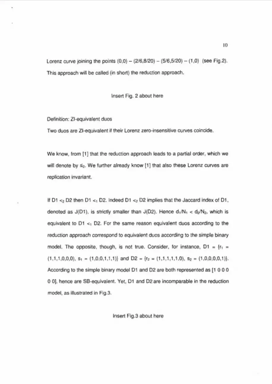
Lorenz curve joining the points (0,O) - (216,8120) - (5/6,5/20) - (1,O) (see Fig.2).

This approach will be called (in short) the reduction approach.

Insert Fig. 2 about here

Definition: ZI-equivalent duos

Two duos are ZI-equivalent if their Lorenz zero-insensitive curves coincide.

We know, from [ I ] that the reduction approach leads to a partial order, which we

will denote by 2,. We further already know [ I ] that also these Lorenz curves are

replication invariant.

If D l q2 D2 then D l <I D2. Indeed D l <2 D2 implies that the Jaccard index of D l ,

denoted as J(DI), is s!rictly smaller than J(D2). Hence ddNl < d21N2, which is

equivalent to D l <, D2. For the same reason equivalent duos according to the

reduction approach correspond to equivalent duos according to the simple binary

model. The opposite, though, is not true. Consider, for instance, D l = {ri =

(1,1,1,0,0,0), sl = (1,0,0,1,1,1)} and D2 = {r2 = (1,1,1,1,1,0), s2 = (1,0,0,0,0,1)].

According to the simple binary model D l and D2 are both represented as [ I 0 0 0

0 01, hence are SB-equivalent. Yet, D l and D2 are incomparable in the reduction

model, as illustrated in Fig.3.

Insert Fig.3 about here

Examples of acceptable similarity measures

As this approach reduces the problem to the zero-insensitive case, we may use

those measures known to be applicable in this case [I ] . Examples of acceptable

measures are the classical similarity measures such as the Jaccard index (equal

to the Gini similarity index), Dice's coefficient, Salton's cosine measure, and the

adapted Simpson index. Expressed in the notation of this article they have the

following mathematical expressions.

The Jaccard index of a duo D is defined here as:

Dice's coefficient of the duo D = {r,s) is:

where p = p+m+l is the number of I s in r* and o =p+m+k is the number of I s in

s*.

Salton's cosine measure of D becomes:

where p and o have the same meaning as for the Dice coefficient.

Finally the adapted Simpson index of D is:

Any strictly increasing function of these measures is again an acceptable

measure in the reduction approach.

The attentive reader may have noticed that we have not yet discussed if the

reduction approach satisfies the requirements PI-P5(a). The reason is that it

does not, at least it does not meet all the requirements. Let us discuss them one

by one. First, because common 0s are encoded as common is , we note that

requirements P I and P2 coincide. These requirements are satisfied by the

reduction approach, as shown in our previous article [I]. Clearly, P5 cannot be

met, and P5a is trivially satisfied. This leaves P3, about adding a (0-1) and P4

about changing a (0-1) by common 0s (here common 1s). P3 is not met as

shown by the following example: we transform D l = {rl = (1,1,1,0,0,0), s, =

(1,0,0,1,1,1)) to D3 = {r3 = (1,1,1,0,0,0,0), s3 = (1,0,0,1,1,1,1)). Then the Lorenz

curves of D l and D3 cross, showing that D l and D3 are not intrinsically

comparable (see Fig. 4).

Insert Fig.4 here

Finally, P4 is satisfied in this approach. Replacing a (0-1) by common 1s always

leads to an intrinsically more similar situation. A proof is provided in the appendix.

5. Third approach: using radix 4 encoding

In this approach common I s are encoded as 3, common 0s as 2, different

symbols as 0s followed by one 1. A duo is then encoded as the number 'zero

point' followed by the code numbers arranged in decreasing order, such as

0.3..32..20..01. All codes of the form 0.3 ... 3 (any number of 3s) are declared

equivalent (corresponding to perfect similarity). Similarly, all codes beginning with

0.0 are declared equivalent (corresponding to the case that not a single symbol

corresponds). For example: D = {r = (1 ,I ,I ,I ,0,0), s = (0,0,1,1,0,l)) is encoded as:

0.3320001, because there are two 1s in common, one 0 in common and three

symbols which are different in the two arrays.

As in the other approaches we declare two duos to be equivalent if they lead to

the same code. This is true for all duos consisting of identical items, but also for,

e.g., D = {r = (1,1,1,1,0,0), s = (0,0,1,1,0,1)), and D'= {r' = (1,1,1,1,0,1), s' =

(0,0,1,1,0,0)). This approach again leads to a complete order on equivalence

classes, denoted as s3.

For similarity considered in this way, the requirements P I , P2, P3, P4 and P5 are

all satisfied: adding common 0s (and certainly Is ) yields a larger code number,

adding 0 -1 decreases the similarity, replacing 0-1 by common 0s yields a larger

code number, replacing common 0s by common 1s also yields a larger code

number. A drawback of this approach is that two identical arrays with at least one

0 are not considered to be completely similar anymore. If they were then

requirement P5, stating that replacing a (0-0) by a (1 -1) makes the arrays more

similar, would not satisfied anymore.

Because only the symbols 3, 2 and 1 and 0 are used these codes can be

considered as numbers in the base or radix 4 number system. In this system,

similar to the better known, binary number system, the number 0.31 corresponds

3 1 to the decimal number -+,=0.8125 , similarly 0.2201 corresponds to

4' 4-

2 2 0 1 -+,+-+-=0.62890625. Note however that if two duos have at least one 4' 4- 4' 44

symbol in common, their decimal representation is at least 0.5. Hence as a

similarity measure we propose the decimal representation minus 0.5, and the

result multiplied by 2. In this way 1 stays 1, namely (1-0.5).2 = 1, while 0.5

becomes (0.5 - 0.5).2 = 0. This proposal has one small inconvenience, namely

that the theory cannot be applied to arrays of length one, because then the duo

{(O),(O)} would have measure 0. But who wants to study the similarity of arrays of

length one?

This encodiny, and hence this approach to similarity, is not duplication invariant,

and duplication increases similarity. In this sense one may say that the radix 4

approach is an approach based on absolute numbers, not on relative proportions

as in the replication invariant cases. Indeed, D5 = {(0,0),(0,0)) is encoded as

0.22; D5 = {(0,0),(1,0)} is encoded as 0.201. Hence D6 s3 D5. However,

replicating D6 twice leads to D7 = ((0,0,0,0),(1 ,I ,0,0)}, which is encoded as

0.22001, so that D6 53 D5 53 D7.

We were not able to find a non-trivial Lorenz curve representation corresponding

to the radix 4 approach. This is not surprising as traditional Lorenz curves are

duplication invariant. Yet, connecting the origin to the point with as abscissa the

decimal representation of the duo's code, and as ordinate the value one, yields -

in a trivial way - a kind of Lorenz curve corresponding with this encoding. As for

the first approach the encoding - in decimal form - corresponds to the Gini

similarity index of this Lorenz curve, but it is possible to consider other

acceptable similarity measures, using the similarity equivalents of the coefficient

of variation, the length of the Lorenz curve, the entropy measure and so on. As

for the first approach, we do not consider these other measures of real practical

value.

6. Different shades of identity

In the previous approach we crossed the thin line between a pure similarity

theory and what we would like to call an 'identity-similarity' theory, as we made a

distinction between different identical duos. From that point of view it certainly

seems artificial to declare all arrays coded as "zero point any number of 3s" to be

'identical'. The same is true for the 0.0 ... 01 case. Of course, the first type of code

represents identical arrays, so they are as similar as possible. The second type

represents completely dissimilar arrays. Yet, taken these codes as they are,

without the extra correction, makes it possible to say that identical arrays with

more i s are more similar than identical arrays with less Is. A similar remark goes

for the dissimilar arrays. We will not go further here into the issue of 'different

shades of identity', as this is not a pure similarity theory anymore.

Notes

a) A generalization

I f the data are not 0 -1 data but categorical data, with no relation at all between

the categories, then the similarity of such a duo can be reduced to the first case,

where a 1 represents the case that categories coincide, and a zero when they do

not. An example: D = { (6, 6 , 6, 6, 6, 6, o), (6, 6, 6 ,6, 6, 6, 6)) is then represented

as[OOOOl 1 O ] = [ l 1 OOOOO].

b) Dichotomizing

Any set of numerical data can be dichotomized in a low and high category. Then

the absence-presence similarity theory presented here can be applied.

c) Another look at the binary case.

In the simple binary model that we presented corresponding zeros as well as

ones were encoded as is . One could imagine an encoding in which only

common ones are encoded as I s. Common zeros are then treated as dissimilar

symbols. The duo D = {r,s) consisting of r = (1 ,I ,I ,I ,0,0) and s = (0,0,1 ,I ,0,1) is

then encoded as [0 0 1 1 0 01 = [I 1 0 0 0 01. As before, d/N (in the encoded

form) seems a reasonable candidate similarity measure. Yet, this approach

violates requirement P2. Adding two common zeros reduces the similarity from

d/N to d/(N+l). For this reason we reject this approach.

d) The zero-insensitive case

Requirements P3 and P4 were not studied in our previous article covering the

zero-insensitive case. The counterexample and proof given here show that also

in the zero-insensitive case P3 is not satisfied, while P4 always is.

e) Lorenz curves

We were able to extend the Lorenz curve approach (as in the reduction to the

insensitive case), but then at least one of the requirements PI-P5 was not

always satisfied. Details can be obtained from the authors. Anyhow, the Lorenz

curves of the second approach must be altered as it is easy to see that adding

common 0s to such a Lorenz curve lifts the curve. This is an unwanted property

as we want to lower this curve in a similarity theory. This shows that the Lorenz

curve approach (at least without alterations) cannot be used for a similarity

theory where common zeros are possible.

f ) The idea of the radix 4 approach may also be applied to the case that common

0s and common I s are considered to be perfectly equal. It suffices to give the

same encoding, e.g. 2, to both (making it a radix 3 approach).

7. Conclusion

In this article we studied similarity for the zero sensitive case of absence-

presence data. A wish list for such a zero-sensitive approach to similarity was

drawn:

P I Adding two common 1s makes two non-identical arrays (strictly) more

similar.

P2 Adding two common 0s makes two non-identical arrays (strictly) more

similar.

P3 Adding a (0-1 ) to a duo makes it (strictly) less similar.

P4 Replacing a (0-1) by a (0-0) makes the arrays (strictly) more similar.

P5 Replacing a (0-0) by a (1 -1) makes the arrays (strictly) more similar,

or the weaker version:

P5a: Replacing a (0-0) by a (1-1) does not alter the similarity between the two

arrays.

Two approaches were given where common 1s and common 0s are treated in

the same way, having the same impact on the similarity of the duo under

consideration. The simple binary case leads to a similarity theory respecting

requirements P1 to P4 of the wish list and P5a. Introducing different weights for

common I s and common Os, leads to an identity-similarity theory. Such a theory

respects all requirements (PI to P5) of the wish list. Examples of functions

respecting the corresponding similarity rankings are given.

Ultimately, any similarity theory is only useful when it helps to understand real-life

examples. We invite our colleagues, not only in the information sciences, but also

in the fields of ecology, sociology and computer sciences, to try out the approach

presented in this article.

References

[ I ] L. Egghe and R. Rousseau, Classical retrieval and overlap measures satisfy

the requirements for rankings based on a Lorenz curve, Information Processing

and Management (2004, to appear).

[2] G. Salton and M.J. McGill, M.J., Introduction to modern information retrieval.

( McGraw-Hill, New York, 1983).

[3] R.E. Tulloss, R.E., Assessment of similarity indices for undesirable properties

and a new tripartite similarity index based on cost functions. In: M.E. Palm and

I.H. Chapela, eds), Mycology in sustainable development: expanding concepts,

vanishing borders (Parkway Publishers, Boone, NC, 1997) pp. 122-143.

[4] D. Nijssen, R. Rousseau and P. Van Hecke, The Lorenz curve: a graphical

representation of evenness, Coenoses, 13(1) (1 998) 33-38.

[5] R.W. Hamming, Error detecting and error correcting codes, Bell Systems

Technical Journal, 29, (1 950) 147-1 60.

[6] P.H.A. Sneath and R.R. Sokal, Numerical taxonomy. (Freeman & Co, San

Francisco, 1973).

Appendix

Proposition 1

The function T= d

, p > 0, is a monotone increasing function of d/N. d + p ( N - d )

Proof. The T-index can be rewritten as: d l N . Writing x for d/N

d l ~ + ~ ( l - d / ~ )

.x gives: T = . Taking the derivative of T with respect to x gives:

.x + p(l - x)

T ' = P , . This expression is always positive, proving that T is a ( x + , ~ x ) ) -

monotone increasing function of dIN.

Proposition 2

Replacing a (0-1) by common I s leads to a Lorenz curve representing an

intrinsically more similar situation.

Proof.

The similarity Lorenz curve is determined by the points with coordinates

S =(?.?] (this point is called the sub-top) and T = (g - . - "i" (the top).

Here d = p+m, p = p+m+l, 0 =p+m+k, and N = p+m+k+l. Replacing (0-1) by

common I s leads either to a situation where d' = p+m+l, p' = p+m+l, a'

=p+m+k+l, and N' = p+m+k+l; or d' = p+m+l , p' = p+m+l+l , a' =p+m+k, and N'

= p+m+k+l. In the first case the new sub-top and top are:

T = -- p - d - l p - d - ' ) , , ( P , G - d ) , and the second case they become: P N a+l

p - d p - d p + l o - d - l S? = [ ----- N ' p + l ) ' i = ( N ' - . Clearly, T , is situated under T, while S

a

and S1 are situated on the same line through the origin. Similarly, S, is situated

under S, while T and T2 are on the same line through the endpoint E with

coordinates (1,O). This shows that the new Lorenz curve depicts an intrinsically

more similar situation than the original one. The proof is illustrated by the

transformation of D l = {rl = (1,1,1,0,0,0), sl = (1,0,0,1,1,l)] to D4 = (r4 =

~1,1!1>0,0,1~, 5.4 = ~1,0,0,1,1!1~~.

Insert Fig.5 about here

Fig.1 Lorenz curve for the simple binary model D = ( r = (1,1,1,1,0,0), s = (O,O,l,l,O,l)),

encoded as [ I 1 1 0 0 01

Fig.2 D = {r = (1,1,1,1,0,0), s = (0,0,1,1 ,O,l)}, is first rewritten as: D' = {r* = ( I , l , l , l , l ,O), s* = (O,O,l ,l , I , I ) } , and then represented by the similarity

Lorenz curve joining the points (0,O) - (216,8120) - (516,5120) - (1,O).

Fig.3 Dl = {rl = (1,1,1,0,0,0), sl = (1,0,0,1,1.1)} and D2 = {r2 = (1 . I ,I , I ,I ,0), s2 = (1,0,0,0,0,1)} are incomparable in the reduction

model, because their Lorenz curves cross

Fig. 4 The transformation of Dl = {r, = (1 , I ,I ,0,0,0), s, = (1,0,0,1 ,I ,I)] to D3 = {r3 = (1,1,1,0,0,0,0), s2 = (1,0,0;1,1,1,1)] (i.e. adding a (0-1)); their Lorenz

curves cross, showing that Dl and D3 are not intrinsically comparable.

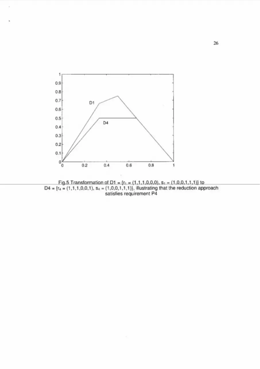
Fig.5 Transformation of Dl = {r, = (1 ,I ,I ,0,0,0), sl = (1,0,0,1,1 ,I)} to D4 = {r4 = (1 , I , I ,0,0,1), s4 = (1,0,0,1 ,I , I)}, illustrating that the reduction approach

satisfies requirement P4