An Efficient Cost Model for Spatial Joins Using R-trees

Yannis Theodoridis Emmanuel Stefanakis Timos Sellis

Computer Science Division

Department of Electrical and Computer Engineering

National Technical University of Athens

Zographou 15773, Athens, Greece

{theodor, stefanak, timos}@cs.ntua.gr

ABSTRACT

Spatial join is one of the fundamental operations in a Spatial Data BaseManagement System. Recently, the family of R-tree-based data structures hasbeen adopted to support the execution of spatial joins. This paper introduces ananalytical model that efficiently estimates the cost (in terms of disk accesses) ofa spatial join query between two spatial datasets. The proposed model is basedon an analytical formula that estimates the cost of the range query using R-trees. In addition, comparison results are presented which show the accuracy ofthe analytical estimations when compared to actual tests on both synthetic andreal datasets. It turns out that the relative error rarely exceeds 15% for allcombinations.

KEYWORDS: Spatial Databases, Query Performance and Optimisation, Spatial Join.

ACKNOWLEDGEMENTS: This research has been partially supported by a research grant fromthe General Secretariat of Research and Technology of Greece (YPER’94) and by theEuropean Commission funded TMR project CHOROCHRONOS.

�

An Efficient Cost Model for Spatial Joins Using R-trees

1. INTRODUCTION

A Spatial Database Management System (SDBMS) is a database management system which(i) offers spatial data types in its data model and query language, and (ii ) supports spatial datatypes in its implementation, providing at least spatial indexing and eff icient algorithms forspatial join [Gut94]. According to the above definition, spatial join is one of the fundamentaloperations supported by an SDBMS. It combines entities from two spatial datasets into singleentities whenever the combination satisfies the spatial join condition (e.g., overlap). In general,the join operation is one of the fundamental database query operations since it retrievesinformation from two different datasets based on their cartesian product.

An example of spatial join is the query “Find all countries in Europe that are crossedby rivers” , or, the more complex one “Find pairs of rivers that cross common countries inEurope and lie west of the 7th meridian” . In the first case, processing the query isstraightforward: the entries of the two spatial datasets C and R (denoting countries and rivers,respectively) are combined on their spatial predicates (polygons ci and lines r j, respectively)

using the topological operator cross. In the latter case, however, there exist several alternativestrategies for processing the query at hand. The first solution consists of the following threesteps: (i) selection of the rivers that lie west of the 7th meridian (using the directional operatorwest) and construction of an intermediate set R1, (ii ) spatial join between R1 and C resulting to

a set S of pairs (r i, cj) of rivers r i that cross countries cj, and (iii ) processing of S in main

memory for pairs (r i, r j), i ≠ j, such that (r i, ci) and (r j, ci) belong to S. Other solutions for this

complex example, which differ on the execution order of the necessary primitive operations andsubsequently the efficiency, are also possible.

Whichever processing algorithm is followed by the spatial query processor of an SDBMSin order to execute a spatial join query, the spatial representations of objects (polygons andlines in the above examples) need to be combined based on a spatial operator, with overlapbeing the most common one. However, the processing of complex spatial representations, suchas polygons, is highly costly. For that reason, the following two-step procedure1 for spatial joinprocessing is usually applied [Ore89]:• filter step: an approximation of each spatial object, such as its minimum bounding rectangle

(MBR), is used in order to produce a set of candidates, a superset of the actual result.• refinement step: each candidate is then examined based on its exact geometry in order to

produce the actual result (usually a CPU-intensive procedure).

The fil ter step is usually based on spatial indexes that organise MBR approximations ofspatial objects [Sam90], whenever it is possible (e.g., spatial join between base datasets andnot intermediate ones), while the refinement step usually includes computational geometrytechniques for the intersection of geometric shapes [PS85].

1 Brinkhoff et al. [BKSS94] alternatively propose a three-step procedure which interferes a second step ofexamining more accurate approximations, e.g., convex hull or minimum m-corner, in order to further reduce theamount of the candidates.

�

Traditional join methods, such as nested loops, sort-merge, or hash join [ME92, EN89],are not eff icient when dealing with spatial data. This is due to the lack of ordering, which is theprimary characteristic of spatial datasets. Because of that, some specialised techniques havebeen proposed: appropriate synchronised tree traversal, for example, when tree indexes exist[Gun93, BKS93] or construction of specialised join indexes on the fly [LR95]. However, thereis a lack of an eff icient cost model which would make an accurate estimation of the I/O cost ofa spatial join operation between two datasets, in correspondance to the existing cost models fora range query between a dataset and a query window, one of the most commonly usedoperations in spatial databases [FK94, TS96].

According to Brinkhoff et al., "... an analytical investigation of the execution time of aspatial join performed with R*-trees seems to be almost impossible ..." [BKS93]. However,this statement was made some years ago and due to the lack of eff icient cost models for R-trees. Such models have recently appeared in the li terature [FK94, TS96] and can be used asthe basic platforms for the analysis of the spatial join operation.

Focusing on hierarchical tree structures, Gunther's proposal [Gun93] was the earliestattempt to provide an analytical model for estimating the cost of spatial joins. Abstractions oftree indexes, called "generalization trees", were modeled on the support of θ-joins.Implementation algorithms for general θ-joins were presented and evaluated for variousprobabili ty distributions. Later, Aref and Samet [AS94] proposed analytical formulas for theexecution cost and the selectivity of spatial joins, based on Kamel and Faloutsos’ R-treeanalysis [KF93]. The basic idea of that work was the consideration of the one dataset as theunderlying database and the other dataset as a source for query windows in order to estimatethe cost of a spatial join query based on the cost of range queries. Experimental results werealso presented to show the accuracy of the selectivity estimation formulas.

In this paper we propose a model that eff iciently estimates the cost (in terms of diskaccesses) of a spatial join query between two spatial datasets. The proposed model is based onthe analytical formula that estimates the cost of a range query, proposed in [TS96]. We alsopresent comparison results that show the accuracy of the analytical estimations when comparedto actual tests on synthetic and real data sets.

The paper is organised as follows: in Section 2 we provide the definition of the spatial joinoperation and we present algorithms for spatial join proposed in the past together with newalternative algorithms. In Section 3 we extend the analytical model introduced in [TS96] whichestimates the cost of a range query (namely the overlap operator) in order to support spatialjoin queries based on the algorithms presented in Section 2. Section 4 contains experimentalresults on synthetic and real datasets that show the accuracy of the proposed model. In Section5 we discuss extensions of the analytical model to also support the cost of other types of spatialjoins (i.e., using operators other than overlap, such as direction or topological operators of highresolution) and a second parameter, the selectivity of a spatial join between two datasets.Finally, we conclude in Section 6, giving also hints for future work.

�

2. BACKGROUND

A join between two relations REL1 and REL2 using a condition REL1[i] θ REL2[j] is one of the

operations supported by Codd's relational model [Cod70]2. The result of the operation containsthose tuples in the cartesian product REL1 × REL2 , where the i-th column of REL1 stands in

relation θ to the j-th column of REL2.

In practical applications, θ is often equali ty, which leads to the equi-join operation. Itsextension for spatial data, called spatial join, applies a spatial operator θ on the i-th column ofREL1 and the j-th column of REL2 which are of some spatial data type. Spatial operators may

be topological (e.g., overlap), directional (e.g., north), or distance-related (e.g., close), with theoverlap operator being the most common one, and spatial data type may include, for example,points, lines, or regions.

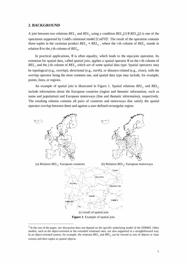
An example of spatial join is ill ustrated in Figure 1. Spatial relations REL1 and REL2

include information about the European countries (region and thematic information, such asname and population) and European motorways (line and thematic information), respectively.The resulting relation contains all pairs of countries and motorways that satisfy the spatialoperator overlap between them and against a user-defined rectangular region.

(a) Relation REL1: European countries (b) Relation REL2: European motorways

(c) result of spatial join

Figure 1: Example of spatial join.

2 In the rest of the paper, our discussion does not depend on the specific underlying model of the SDBMS. Othermodels, such as the object-oriented or the extended relational ones, are also supported in a straightforward way.In an object-oriented system, for example, the relations REL1 and REL2 can be viewed as sets of objects or class

extents and their tuples as spatial objects.

�

Implementations of the traditional join operation include simple techniques, such as nestedloops, as well as more eff icient techniques, such as sort-merge or hash methods (see [ME92]for a survey). Unfortunately, the above techniques are not eff icient for spatial data which arecharacterised by the absence of total ordering, a necessary condition for all previoustechniques. Although several extensions of the traditional methods have been proposed [Ore89,Rot91], recent research efforts have focused on methods dedicated to spatial data.

The proposals which can be found in the li terature are grouped in three categories:methods that consider the existence of spatial indexes on (i) none, (ii ) one, (iii ) both relationsREL1 and REL2. In the first case, where no pre-constructed indexes exist, relevant proposals

adopt the usage of rectangle intersection algorithms available in computational geometry[BG92]; the extension of the sort-merge [PD96] or the hash join [LR96] techniques; or theconstruction of special tree indexes on the fly, e.g., seeded trees in [LR95]. In the second case,where one spatial index, an R-tree for example, is maintained for the first dataset, Lo andRavishankar [LR94] propose the construction of a seeded tree on the second dataset, usinginformation of the existing index.

In the rest of the paper we will consider the third case, in which both relations aresupported by spatial indexes. Since the processing of spatial predicates in a spatial relation iscrucial in an SDBMS one can argue that indexes on those predicates should necessarily exist inorder to eff iciently support the basic (spatial) operations of the system. Among others, Gridfiles have been studied in [Rot91, BHF93] and R-trees in [BKS93]. We select the R-treestructure to be the underlying index since it has been widely recognised as the most effectiveindexing method and has been incorporated in commercial database systems, such as Postgres[SRH90] and Illustra [Ube94].

The basic idea on the implementation of spatial joins using R-trees is the synchronisedtraversal of the two index structures. We present next a brief description of the R-tree indexand the implementation of spatial joins between two relations indexed by two R-trees.

2.1. Spatial join between two R-trees

The R-tree [Gut84, BKSS90] is a height-balanced tree which consists of intermediate and leafnodes. A leaf node is of the form

(oid, RECT)where oid is an object identifier and it is used to refer to an object in the database. RECT is theMBR approximation of the data object, i.e., it is of the form

(pl-1, pl-2, …, pl-n, pu-1, pu-2, …, pu-n)

which represents the 2n coordinates of the lower-left (pl) and the upper-right (pu) corner of a n-

dimensional (hyper-) rectangle p. An intermediate node is of the form(ptr, RECT)

where ptr is a pointer to a lower level node of the tree and RECT is a representation of therectangle that encloses.

Let M be the maximum number of entries in a node and let m ≤ M/2 be a parameterspecifying the minimum number of entries in a node. An R-tree satisfies the followingproperties:

�

(i) Every leaf node contains between m and M entries unless it is the root.(ii ) For each entry (oid, MBR) in a leaf node, RECT is the smallest rectangle that spatially

contains the data object represented by oid.(iii ) Every intermediate node has between m and M children unless it is the root.(iv) For each entry (ptr, RECT) in an intermediate node, RECT is the smallest rectangle that

spatially contains the rectangles in the child node.(v) The root node has at least two children unless it is a leaf.(vi) All leaves appear in the same level of the tree.

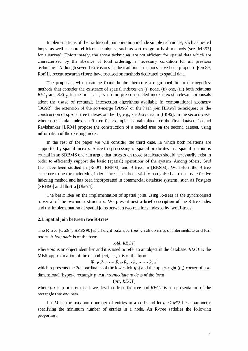
Figure 2 shows an example set of data rectangles and the corresponding R-tree buil t onthese rectangles (assuming maximum node capacity M = 4).

A

B

C

D

E

F

HI

K

J

M

NL

G

A B C

D E F G H I J K L M N

√

√ √

q

A B C

ROOT

Figure 2: An example of R-tree index.

The range query operation, which retrieves all objects of a spatial relation REL thatoverlap a query window q, one of the most common operations in spatial applications, isimplemented using a traversal of the R-tree index: starting from the root node, a tree traversalis performed according to the result of the overlap operation between q and the root noderectangles. If the result (i.e., the overlap area) is not empty then the traversal continues to thesubtree rooted by that node, otherwise it stops. When the algorithm reaches the data rectangles,all data items which overlap the query window q are added to the answer set (in the example ofFigure 2 three out of four nodes, namely 5227, $, and %, are accessed, and one data rectangle,namely *, qualifies for the answer set).

The spatial join operation between two spatial relations REL1 and REL2 can be supported

by applying synchronised tree traversals on both R-tree indexes. A technique based on thisgeneral idea was originally introduced by Brinkhoff et al. in [BKS93]. Specifically, for two R-tree indexes rooted by nodes R1 and R2, respectively, the procedure of spatial join is the

following:

�

6-�5��5���5BQRGH��� � �6SDWLDO-RLQ�$OJRULWKP�IRU�5�WUHHV�RI�WKH�VDPHKHLJKW� �

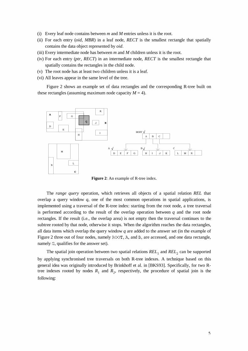
�� %(*,1�� )25��DOO�(U��LQ�5���'2�� )25��DOO�(U��LQ�5���'2�� ,)��RYHUODS�(U��UHFW��(U��UHFW���7+(1�� ,)��5��LV�D�OHDI�SDJH��7+(1�� RXWSXW�(U��RLG��(U��RLG��� (/6(�� 5HDG3DJH�(U��SWU���5HDG3DJH�(U��SWU���� 6-�(U��SWU��(U��SWU��� (1'�,)�� (1'�,)�� (1'�)25�� (1'�)25��� (1'�

Figure 3: The spatial join algorithm for trees of the same height

In other words, a synchronised traversal of both R-trees is performed with the entries ofnodes R1 and R2 playing the roles of query rectangles and data rectangles in a series of range

queries. The cost of a spatial join operation is measured by the total amount of actual diskaccesses for both disk-resident indexes (the procedure 5HDG3DJH either performs an actualread operation on the disk or reads the corresponding node information from a buffer thatmaintains the current path for each tree).

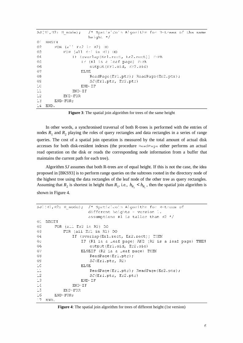
Algorithm SJ assumes that both R-trees are of equal height. If this is not the case, the ideaproposed in [BKS93] is to perform range queries on the subtrees rooted in the directory node ofthe highest tree using the data rectangles of the leaf node of the other tree as query rectangles.Assuming that R2 is shortest in height than R1, i.e., h hR R2 1

< , then the spatial join algorithm is

shown in Figure 4.

6-��5��5���5BQRGH��� � �6SDWLDO-RLQ�$OJRULWKP�IRU�5�WUHHV�RIGLIIHUHQW�KHLJKWV���YHUVLRQ���DVVXPSWLRQ��5��LV�WDOOHU�WKDQ�5�� �

�� %(*,1�� )25��DOO�(U��LQ�5���'2�� )25��DOO�(U��LQ�5���'2�� ,)��RYHUODS�(U��UHFW��(U��UHFW���7+(1�� ,)��5��LV�D�OHDI�SDJH��$1'��5��LV�D�OHDI�SDJH��7+(1�� RXWSXW�(U��RLG��(U��RLG��� (/6(,)��5��LV�D�OHDI�SDJH��7+(1�� 5HDG3DJH�(U��SWU���� 6-�(U��SWU��5���� (/6(�� 5HDG3DJH�(U��SWU���5HDG3DJH�(U��SWU���� 6-�(U��SWU��(U��SWU��� (1'�,)�� (1'�,)�� (1'�)25�� (1'�)25��� (1'�

Figure 4: The spatial join algorithm for trees of different height (1st version)

�

Algorithm SJ1 is identical to SJ when R1 and R2 are intermediate nodes, and differentiates,

by introducing lines 07 thru 09, to handle the case of R1 being an intermediate node and R2 a

leaf node. In this case, the idea is to perform range queries on the subtrees rooted by R1 using

the data rectangles of R2 as query windows.

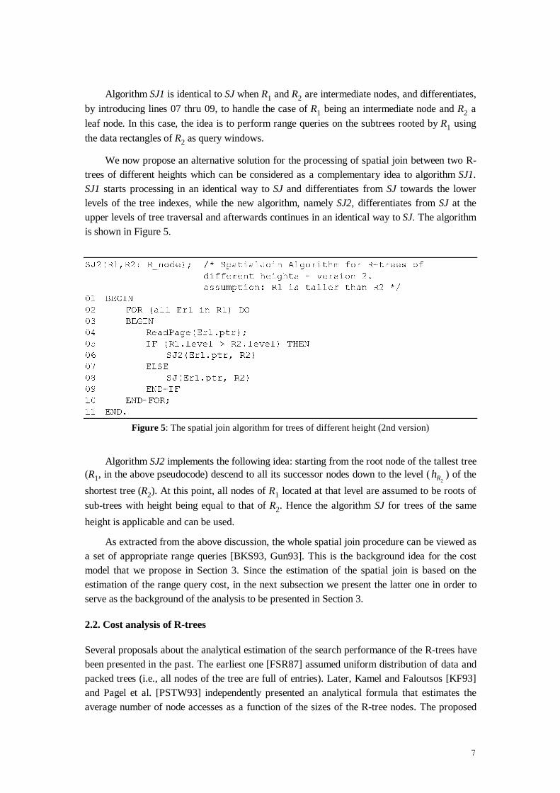
We now propose an alternative solution for the processing of spatial join between two R-trees of different heights which can be considered as a complementary idea to algorithm SJ1.SJ1 starts processing in an identical way to SJ and differentiates from SJ towards the lowerlevels of the tree indexes, while the new algorithm, namely SJ2, differentiates from SJ at theupper levels of tree traversal and afterwards continues in an identical way to SJ. The algorithmis shown in Figure 5.

6-��5��5���5BQRGH��� � �6SDWLDO-RLQ�$OJRULWKP�IRU�5�WUHHV�RIGLIIHUHQW�KHLJKWV���YHUVLRQ���DVVXPSWLRQ��5��LV�WDOOHU�WKDQ�5�� �

�� %(*,1�� )25��DOO�(U��LQ�5���'2�� %(*,1�� 5HDG3DJH�(U��SWU���� ,)��5��OHYHO�!�5��OHYHO��7+(1�� 6-��(U��SWU��5���� (/6(�� 6-�(U��SWU��5���� (1'�,)�� (1'�)25��� (1'�

Figure 5: The spatial join algorithm for trees of different height (2nd version)

Algorithm SJ2 implements the following idea: starting from the root node of the tallest tree(R1, in the above pseudocode) descend to all i ts successor nodes down to the level (hR2

) of the

shortest tree (R2). At this point, all nodes of R1 located at that level are assumed to be roots of

sub-trees with height being equal to that of R2. Hence the algorithm SJ for trees of the same

height is applicable and can be used.

As extracted from the above discussion, the whole spatial join procedure can be viewed asa set of appropriate range queries [BKS93, Gun93]. This is the background idea for the costmodel that we propose in Section 3. Since the estimation of the spatial join is based on theestimation of the range query cost, in the next subsection we present the latter one in order toserve as the background of the analysis to be presented in Section 3.

2.2. Cost analysis of R-trees

Several proposals about the analytical estimation of the search performance of the R-trees havebeen presented in the past. The earliest one [FSR87] assumed uniform distribution of data andpacked trees (i.e., all nodes of the tree are full of entries). Later, Kamel and Faloutsos [KF93]and Pagel et al. [PSTW93] independently presented an analytical formula that estimates theaverage number of node accesses as a function of the sizes of the R-tree nodes. The proposed

�

formula is quali tative, i.e., it does not really predict the average number of node accesses but,intuitively, presents the effects of the sizes of the nodes and the query window to theperformance of the R-tree.

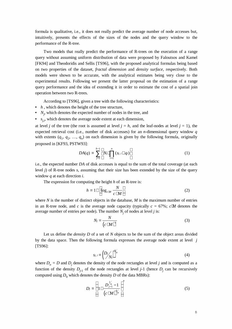
Two models that really predict the performance of R-trees on the execution of a rangequery without assuming uniform distribution of data were proposed by Faloutsos and Kamel[FK94] and Theodoridis and Selli s [TS96], with the proposed analytical formulas being basedon two properties of the dataset, fractal dimension and density surface, respectively. Bothmodels were shown to be accurate, with the analytical estimates being very close to theexperimental results. Following we present the latter proposal on the estimation of a rangequery performance and the idea of extending it in order to estimate the cost of a spatial joinoperation between two R-trees.

According to [TS96], given a tree with the following characteristics:• h , which denotes the height of the tree structure,• Nj, which denotes the expected number of nodes in the tree, and

• sj,i, which denotes the average node extent at each dimension,

at level j of the tree (the root is assumed at level j = h, and the leaf-nodes at level j = 1), theexpected retrieval cost (i.e., number of disk accesses) for an n-dimensional query window qwith extents (q1, q2, …, qn) on each dimension is given by the following formula, originally

proposed in [KF93, PSTW93]:

DA q N s qj j i i

i

n

j

h

( ) ( ),= ⋅ +

==

−

∏∑11

1

(1)

i.e., the expected number DA of disk accesses is equal to the sum of the total coverage (at eachlevel j) of R-tree nodes s, assuming that their size has been extended by the size of the querywindow q at each direction i.

The expression for computing the height h of an R-tree is:

hN

c Mc M= +⋅

⋅1 log (2)

where N is the number of distinct objects in the database, M is the maximum number of entriesin an R-tree node, and c is the average node capacity (typically c = 67%; c⋅M denotes theaverage number of entries per node). The number Nj of nodes at level j is:

( )N

N

c Mj

j=⋅

(3)

Let us define the density D of a set of N objects to be the sum of the object areas dividedby the data space. Then the following formula expresses the average node extent at level j[TS96]:

( )s DNj i

j

j

n, =

1

(4)

where Do = D and Dj denotes the density of the node rectangles at level j and is computed as a

function of the density Dj-1 of the node rectangles at level j-1 (hence Dj can be recursively

computed using D0 which denotes the density D of the data MBRs):

( )D

D

c Mj

jn

n

n

= +−

⋅

−111

1

1(5)

�

Quali tatively, the cost model estimates the retrieval cost (i.e., number of disk accesses) foran n-dimensional query window q, based on the knowledge of the data set (i.e., the number Nof data objects and the density D of their MBRs) and the query window extents (q1, q2, …, qn)

only.

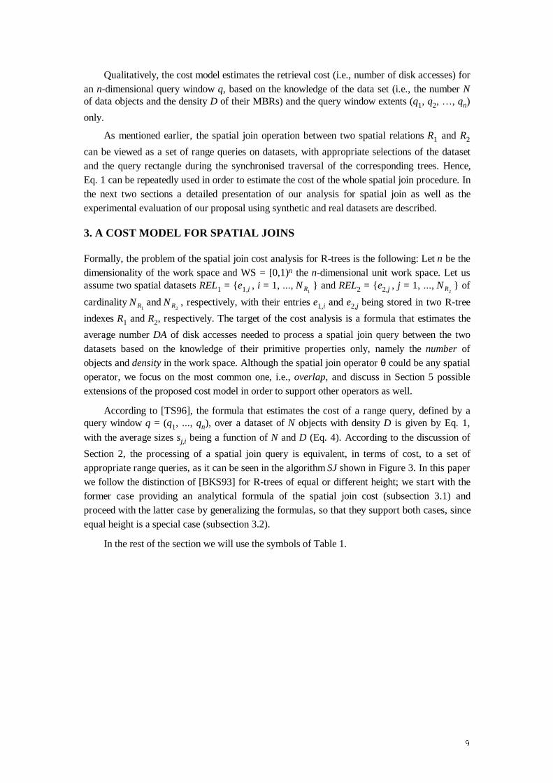
As mentioned earlier, the spatial join operation between two spatial relations R1 and R2

can be viewed as a set of range queries on datasets, with appropriate selections of the datasetand the query rectangle during the synchronised traversal of the corresponding trees. Hence,Eq. 1 can be repeatedly used in order to estimate the cost of the whole spatial join procedure. Inthe next two sections a detailed presentation of our analysis for spatial join as well as theexperimental evaluation of our proposal using synthetic and real datasets are described.

3. A COST MODEL FOR SPATIAL JOINS

Formally, the problem of the spatial join cost analysis for R-trees is the following: Let n be thedimensionali ty of the work space and WS = [0,1)n the n-dimensional unit work space. Let usassume two spatial datasets REL1 = { e1,i , i = 1, ...,NR1

} and REL2 = { e2,j , j = 1, ...,NR2} of

cardinali ty NR1andNR2

, respectively, with their entries e1,i and e2,j being stored in two R-tree

indexes R1 and R2, respectively. The target of the cost analysis is a formula that estimates the

average number DA of disk accesses needed to process a spatial join query between the twodatasets based on the knowledge of their primitive properties only, namely the number ofobjects and density in the work space. Although the spatial join operator θ could be any spatialoperator, we focus on the most common one, i.e., overlap, and discuss in Section 5 possibleextensions of the proposed cost model in order to support other operators as well.

According to [TS96], the formula that estimates the cost of a range query, defined by aquery window q = (q1, ..., qn), over a dataset of N objects with density D is given by Eq. 1,

with the average sizes sj,i being a function of N and D (Eq. 4). According to the discussion of

Section 2, the processing of a spatial join query is equivalent, in terms of cost, to a set ofappropriate range queries, as it can be seen in the algorithm SJ shown in Figure 3. In this paperwe follow the distinction of [BKS93] for R-trees of equal or different height; we start with theformer case providing an analytical formula of the spatial join cost (subsection 3.1) andproceed with the latter case by generalizing the formulas, so that they support both cases, sinceequal height is a special case (subsection 3.2).

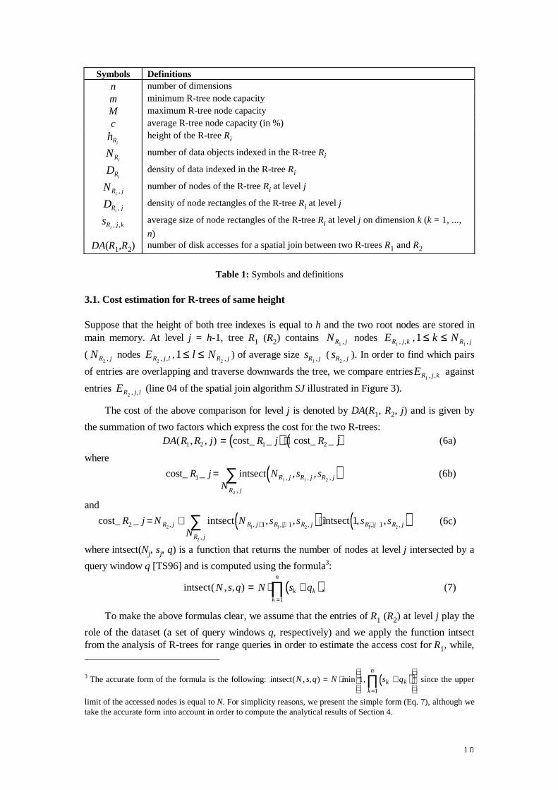
In the rest of the section we will use the symbols of Table 1.

��

Symbols Definitionsn number of dimensions

m minimum R-tree node capacity

M maximum R-tree node capacity

c average R-tree node capacity (in %)

hRiheight of the R-tree Ri

NRinumber of data objects indexed in the R-tree Ri

DRidensity of data indexed in the R-tree Ri

NR ji ,number of nodes of the R-tree Ri at level j

DR ji ,density of node rectangles of the R-tree Ri at level j

sR j ki , ,average size of node rectangles of the R-tree Ri at level j on dimension k (k = 1, ...,

n)DA(R1,R2) number of disk accesses for a spatial join between two R-trees R1 and R2

Table 1: Symbols and definitions

3.1. Cost estimation for R-trees of same height

Suppose that the height of both tree indexes is equal to h and the two root nodes are stored inmain memory. At level j = h-1, tree R1 (R2) contains NR j1 , nodes ER j k1 , , ,1

1≤ ≤k NR j,

( NR j2 , nodes ER j l2 , , ,12

≤ ≤l NR j, ) of average size sR j1 , ( sR j2 , ). In order to find which pairs

of entries are overlapping and traverse downwards the tree, we compare entriesER j k1 , , against

entries ER j l2 , , (line 04 of the spatial join algorithm SJ illustrated in Figure 3).

The cost of the above comparison for level j is denoted by DA(R1, R2, j) and is given by

the summation of two factors which express the cost for the two R-trees:

( ) ( )DA R R j R j R j( , , )1 2 1 2= +cost_ _ cost_ _ (6a)

where

( )cost_ _ intsectR j N s sN

R j R j R j

R j

1 1 1 2

2

= ∑ , , ,

,

, , (6b)

and

( ) ( )cost_ _ intsect intsectR j N N s sN

s sR j R j R j R j

R j

R j R j2 1 1 12 1 1 2

2

1 21= + ⋅+ + +∑, , , ,

,

, ,, , , , (6c)

where intsect(Nj, sj, q) is a function that returns the number of nodes at level j intersected by a

query window q [TS96] and is computed using the formula3:

( )intsect( , , )N s q N s qk kk

n

= ⋅ +=

∏1

, (7)

To make the above formulas clear, we assume that the entries of R1 (R2) at level j play the

role of the dataset (a set of query windows q, respectively) and we apply the function intsectfrom the analysis of R-trees for range queries in order to estimate the access cost for R1, while,

3 The accurate form of the formula is the following: ( )intsect( , , ) min ,N s q N s qk kk

n

= ⋅ +

=∏1

1

since the upper

limit of the accessed nodes is equal to N. For simpli city reasons, we present the simple form (Eq. 7), although wetake the accurate form into account in order to compute the analytical results of Section 4.

��

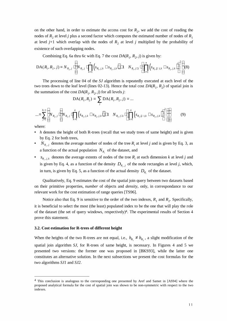
on the other hand, in order to estimate the access cost for R2, we add the cost of reading the

nodes of R2 at level j plus a second factor which computes the estimated number of nodes of R1

at level j+1 which overlap with the nodes of R2 at level j multiplied by the probabili ty of

existence of such overlapping nodes.

Combining Eq. 6a thru 6c with Eq. 7 the cost DA(R1, R2, j) is given by:

( ) ( )DA( , , ) , , , , , , , , , , ,R R j N N s s N s sR j R j R j k R j kk

n

R j R j k R j kk

n

1 21

1 11

2

2 1 1 2 1 1 21= ⋅ ⋅ + + + ⋅ +

=+ +

=∏ ∏ (8)

The processing of line 04 of the SJ algorithm is repeatedly executed at each level of thetwo trees down to the leaf level (lines 02-13). Hence the total cost DA(R1, R2) of spatial join is

the summation of the cost DA(R1, R2, j) for all levels j:

DA DA( , ) ( , , ) ...R R R R jj

1 2 1 2= =∑

( ) ( )... , , , , , , , , , , ,= ⋅ ⋅ + + + ⋅ +

=+ +

==

−

∏ ∏∑ N N s s N s sR j R j R j k R j kk

n

R j R j k R j kk

n

j

h

2 1 1 2 1 1 21

1 11

2

1

1

1 (9)

where:• h denotes the height of both R-trees (recall that we study trees of same height) and is given

by Eq. 2 for both trees,• NR ji , denotes the average number of nodes of the tree Ri at level j and is given by Eq. 3, as

a function of the actual population NRi of the dataset, and

• sR j ki , , denotes the average extents of nodes of the tree Ri at each dimension k at level j and

is given by Eq. 4, as a function of the density DR ji , of the node rectangles at level j, which,

in turn, is given by Eq. 5, as a function of the actual density DRi of the dataset.

Quali tatively, Eq. 9 estimates the cost of the spatial join query between two datasets basedon their primitive properties, number of objects and density, only, in correspondance to ourrelevant work for the cost estimation of range queries [TS96].

Notice also that Eq. 9 is sensitive to the order of the two indexes, R1 and R2. Specifically,

it is beneficial to select the most (the least) populated index to be the one that will play the roleof the dataset (the set of query windows, respectively)4. The experimental results of Section 4prove this statement.

3.2. Cost estimation for R-trees of different height

When the heights of the two R-trees are not equal, i.e., h hR R1 2≠ , a slight modification of the

spatial join algorithm SJ, for R-trees of same height, is necessary. In Figures 4 and 5 wepresented two versions: the former one was proposed in [BKS93], while the latter oneconstitutes an alternative solution. In the next subsections we present the cost formulas for thetwo algorithms SJ1 and SJ2.

4 This conclusion is analogous to the corresponding one presented by Aref and Samet in [AS94] where theproposed analytical formula for the cost of spatial join was shown to be non-symmetric with respect to the twoindexes.

��

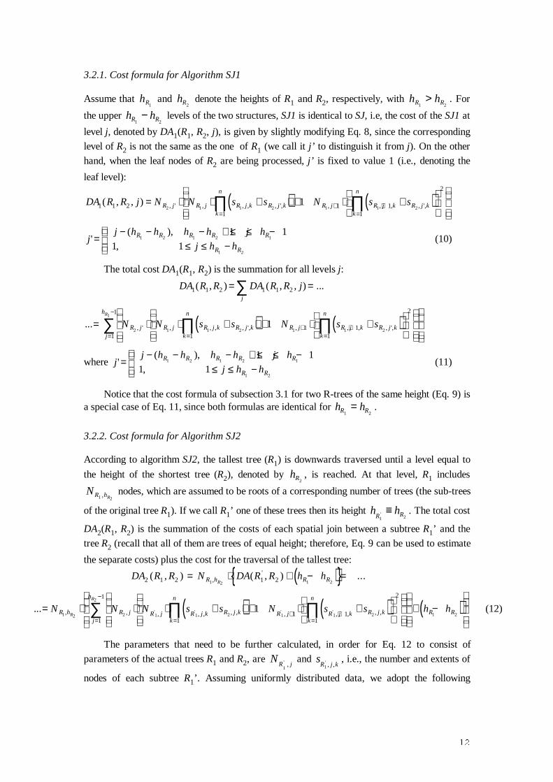
3.2.1. Cost formula for Algorithm SJ1

Assume that hR1 and hR2

denote the heights of R1 and R2, respectively, with h hR R1 2> . For

the upper h hR R1 2− levels of the two structures, SJ1 is identical to SJ, i.e, the cost of the SJ1 at

level j, denoted by DA1(R1, R2, j), is given by slightly modifying Eq. 8, since the corresponding

level of R2 is not the same as the one of R1 (we call i t j’ to distinguish it from j). On the other

hand, when the leaf nodes of R2 are being processed, j’ is fixed to value 1 (i.e., denoting the

leaf level):

( ) ( )DA R R j N N s s N s sR j R j R j k R j kk

n

R j R j k R j kk

n

1 1 21

1 11

2

2 1 1 2 1 1 21( , , ) , ' , , , , ', , , , , ',= ⋅ ⋅ + + + ⋅ +

=+ +

=∏ ∏

jj h h

j h h h h j h

R R

R R R R R',

( ),=

≤ ≤ −− − − + ≤ ≤ −

1 1

1 1

1 2

1 2 1 2 1 (10)

The total cost DA1(R1, R2) is the summation for all levels j:

DA R R DA R R jj

1 1 2 1 1 2( , ) ( , , ) ...= =∑

( ) ( )... , ' , , , , ', , , , , ',= ⋅ ⋅ + + + ⋅ +

=+ +

==

−

∏ ∏∑ N N s s N s sR j R j R j k R j kk

n

R j R j k R j kk

n

j

hR

2 1 1 2 1 1 2

1

11 1

1

2

1

1

1

where jj h h

j h h h h j h

R R

R R R R R',

( ),=

≤ ≤ −− − − + ≤ ≤ −

1 1

1 1

1 2

1 2 1 2 1 (11)

Notice that the cost formula of subsection 3.1 for two R-trees of the same height (Eq. 9) isa special case of Eq. 11, since both formulas are identical for h hR R1 2

= .

3.2.2. Cost formula for Algorithm SJ2

According to algorithm SJ2, the tallest tree (R1) is downwards traversed until a level equal to

the height of the shortest tree (R2), denoted by hR2, is reached. At that level, R1 includes

NR hR1 2, nodes, which are assumed to be roots of a corresponding number of trees (the sub-trees

of the original tree R1). If we call R1’ one of these trees then its height h hR R

1 2' ≡ . The total cost

DA2(R1, R2) is the summation of the costs of each spatial join between a subtree R1’ and the

tree R2 (recall that all of them are trees of equal height; therefore, Eq. 9 can be used to estimate

the separate costs) plus the cost for the traversal of the tallest tree:

( ){ }DA R R N DA R R h hR h R RR2 1 2 1 21 2 1 2( , ) ( , ) ...,

'= ⋅ + − =

( ) ( ) ( )... , , , , , , , , , , , ,' ' ' '= ⋅ ⋅ ⋅ + + + ⋅ +

+ −

=+ +

==

−

∏ ∏∑N N N s s N s s h hR h R j R j R j k R j kk

n

R j R j k R j kk

n

j

h

R RR

R

1 2 2 1 1 2 1 1 2

2

1 21

11 1

1

2

1

1

(12)

The parameters that need to be further calculated, in order for Eq. 12 to consist of

parameters of the actual trees R1 and R2, are NR j

1' ,

and sR j k1

' , ,, i.e., the number and extents of

nodes of each subtree R1’ . Assuming uniformly distributed data, we adopt the following

��

formulas for the two parameters as functions of the actual NR j

1,

and sR j k1 , ,

parameters (it is

easy to verify the correctness of those formulas):

s sR j k R j k1 1

' , , , ,= (13)

and NN

NR j

R j

R hR1

1

1 2

' ,

,

,

= , (14)

where( )

NN

c MR h

R

hR R1 2

1

2, =

⋅

(15)

Again notice that Eq. 9 is also a special case of Eq. 12, since the assumptionh hR R1 2

= leads to the equality NR hR1 21, = (i.e., the root node).

The analytical comparison of the two algorithms SJ1 and SJ2 for R-trees of differentheight is not straightforward since Eq. 11 and Eq. 12 are not easily comparable. However,according to our experiments which are presented in Section 4, we conclude that the twoalgorithms are almost equivalent for both experimental and analytical performance results.

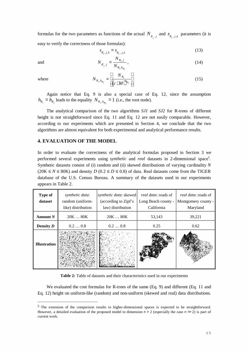
4. EVALUATION OF THE MODEL

In order to evaluate the correctness of the analytical formulas proposed in Section 3 weperformed several experiments using synthetic and real datasets in 2-dimensional space5.Synthetic datasets consist of (i) random and (ii ) skewed distributions of varying cardinali ty N(20K ≤ N ≤ 80K) and density D (0.2 ≤ D ≤ 0.8) of data. Real datasets come from the TIGERdatabase of the U.S. Census Bureau. A summary of the datasets used in our experimentsappears in Table 2.

Type of

dataset

synthetic data:

random (uniform-

like) distribution

synthetic data: skewed

(according to Zipf’s

law) distribution

real data: roads of

Long Beach county -

California

real data: roads of

Montgomery county -

Maryland

Amount N 20K … 80K 20K … 80K 53,143 39,221

Density D 0.2 … 0.8 0.2 … 0.8 0.25 0.62

Illustration

Table 2: Table of datasets and their characteristics used in our experiments

We evaluated the cost formulas for R-trees of the same (Eq. 9) and different (Eq. 11 andEq. 12) height on uniform-like (random) and non-uniform (skewed and real) data distributions.

5 The extension of the comparison results to higher-dimensional spaces is expected to be straightforward.However, a detailed evaluation of the proposed model to dimension n > 2 (especiall y the case n >> 2) is part ofcurrent work.

��

For the experimental tests we buil t R*-tree [BKSS94] indexes and performed several spatialjoins using the datasets of Table 2. On the other hand, the analytical results were based on Eq.9, Eq. 11 and Eq. 12 with the average capacity of the tree indexes being set to the typical c =67% value.

Especially for non-uniform distributions of data, a transformation of the actual density ofeach dataset was necessary. We replaced the actual density DRi

by the “effective” density

DRi

' in the highly-populated part of the work space (as an example, for skewed datasets

following the 80:20 law, the appropriate transformation is D DR Ri i

' = ⋅4 ).

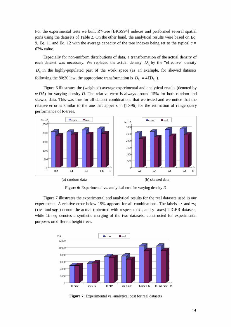
Figure 6 ill ustrates the (weighted) average experimental and analytical results (denoted byw.DA) for varying density D. The relative error is always around 15% for both random andskewed data. This was true for all dataset combinations that we tested and we notice that therelative error is similar to the one that appears in [TS96] for the estimation of range queryperformance of R-trees.

0,2 0,4 0,6 0,80

500

1000

1500

2000

2500

w. DA

0,2 0,4 0,6 0,8

exper. anal.

D 0,2 0,4 0,6 0,80

500

1000

1500

2000

2500

3000

w. DA

0,2 0,4 0,6 0,8

exper. anal.

D

(a) random data (b) skewed data

Figure 6: Experimental vs. analytical cost for varying density D

Figure 7 ill ustrates the experimental and analytical results for the real datasets used in ourexperiments. A relative error below 15% appears for all combinations. The labels OE and PJ(OE¶ and PJ¶) denote the actual (mirrored with respect to x-, and y- axes) TIGER datasets,while OE�PJ denotes a synthetic merging of the two datasets, constructed for experimentalpurposes on different height trees.

lb / mg mg / lb lb / lb' mg / mg' lb+mg / lb' lb+mg / mg'0

2000

4000

6000

8000

10000

12000

lb / mg mg / lb lb / lb' mg / mg' lb+mg / lb' lb+mg / mg'

exper. anal.

D

DA

Figure 7: Experimental vs. analytical cost for real datasets

��

According to our experiments on both synthetic and real datasets it turns out that the costformulas presented in Section 3 are non-symmetric, a fact that has been already mentionedduring the presentation of the cost model. Comparison results (not presented due to spacelimitations) confirm that the choice of the smaller (larger) dataset to play the role of queries(data) is the best choice for the effectiveness of the algorithms.

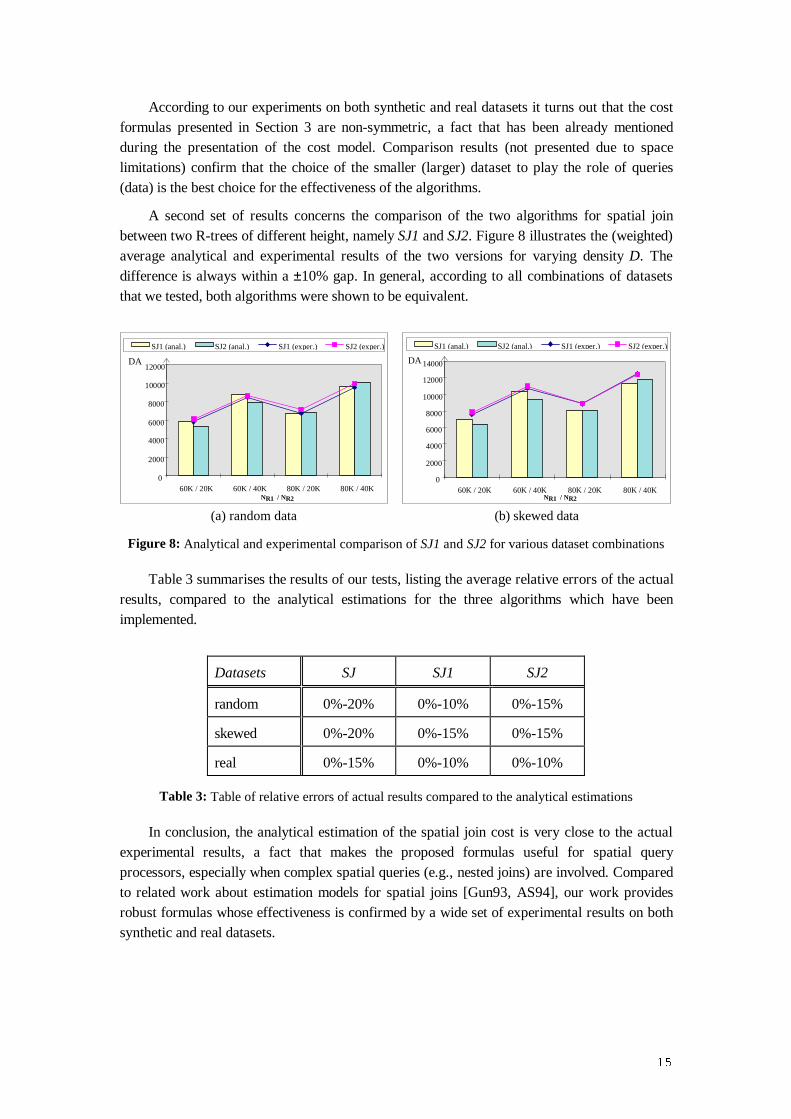
A second set of results concerns the comparison of the two algorithms for spatial joinbetween two R-trees of different height, namely SJ1 and SJ2. Figure 8 ill ustrates the (weighted)average analytical and experimental results of the two versions for varying density D. Thedifference is always within a ±10% gap. In general, according to all combinations of datasetsthat we tested, both algorithms were shown to be equivalent.

0

2000

4000

6000

8000

10000

12000

60K / 20K 60K / 40K 80K / 20K 80K / 40K

SJ1 (anal.) SJ2 (anal.) SJ1 (exper.) SJ2 (exper.)

DA

NR1 / NR2

0

2000

4000

6000

8000

10000

12000

14000

60K / 20K 60K / 40K 80K / 20K 80K / 40K

SJ1 (anal.) SJ2 (anal.) SJ1 (exper.) SJ2 (exper.)

DA

NR1 / NR2

(a) random data (b) skewed data

Figure 8: Analytical and experimental comparison of SJ1 and SJ2 for various dataset combinations

Table 3 summarises the results of our tests, listing the average relative errors of the actualresults, compared to the analytical estimations for the three algorithms which have beenimplemented.

Datasets SJ SJ1 SJ2

random 0%-20% 0%-10% 0%-15%

skewed 0%-20% 0%-15% 0%-15%

real 0%-15% 0%-10% 0%-10%

Table 3: Table of relative errors of actual results compared to the analytical estimations

In conclusion, the analytical estimation of the spatial join cost is very close to the actualexperimental results, a fact that makes the proposed formulas useful for spatial queryprocessors, especially when complex spatial queries (e.g., nested joins) are involved. Comparedto related work about estimation models for spatial joins [Gun93, AS94], our work providesrobust formulas whose effectiveness is confirmed by a wide set of experimental results on bothsynthetic and real datasets.

��

5. DISCUSSION

In this work we have considered overlap to be the θ operator of the θ-join operation. Anyspatial operator could be used instead. For instance:• topological operators: overlap, meet, covers, contains, equal, etc.• direction operators: north, northeast, etc.• distance operators: within x, near, nearest, etc.

Two questions arise: (i) which are the necessary transformations on the analytical modelin order to support a spatial operator other than overlap, and (ii ) is overlap representative forthe accuracy of the estimation cost of a spatial join between two indexed datasets? To sketch ananswer to the above (their extensive study is part of our current work) we discuss somerelevant results from the literature:(i) As discussed in [PTSE95, PT97], in order to use R-trees for the retrieval of a spatial

operator OP instead of the range query (i.e., the overlap operator) we need to construct aquery window Q as a transformation of the actual query window q and compare it witheach node rectangle P while traversing the R-tree. Formally, OP(P,q) ⇒ overlap(P,Q).The above transformation also works well for the analytical estimation of the range querycost since the relative error of the estimation is similar to that of range queries [TP95].Hence we argue that the above transformation could also work well for spatial joins.

(ii ) The representativeness of the overlap operator for the accuracy of the spatial join costestimation is analogous to its representativeness for the accuracy of the range query costestimation since we implement spatial join as a series of appropriate range queries. Inaddition, recent research shows that range (window) queries can widely be regarded asrepresentative for other (e.g., enclosure, containment) queries for a wide range of regionsize [PS96]. Considering that work as background we could study its adoption also forspatial join.

Currently, the proposed model supports the cost (in terms of disk accesses) of a spatialjoin query between two datasets. A second parameter which could also be supported is theselectivity of spatial join. Formally, the selectivity S(R1,R2) of a spatial join between two R-

trees R1 and R2 is defined to be the ratio of the number of items in the answer set (i.e., the

overlapping pairs of entries (e1,i, e2,j) when assuming overlap to be the join operator) over the

cartesian product R1 × R2. Selectivity estimation [Chr83, PC84], in general, is useful to spatial

query optimisers when the result of a query is input to another query, and so on; in such cases,estimation of the cardinali ty of the answer set is an important factor in order to decide for theexecution order of complex queries (i.e., procedures).

Assuming uniform distribution of data and based on the corresponding formula for theestimation of range query selectivity proposed in [TS96], the formula that estimates the numberof overlapping pairs of objects at leaf levels of R1 and R2 is the following:

( ) ( )#overlappingpairs intsect= = ⋅ ⋅ +∑ ∏=

N s sN

N N s sR R R

R

R R R k R kk

n

1 1 2

2

1 2 1 2

1

, , , , (16)

We consider the data rectangles of the first dataset playing the role of query windows on adataset composed by the data rectangles of the second. Combining Eq. 16 with Eq. 4 theformula for the expected selectivity S(R1,R2) is:

��

( )S R RN N

s sR R

R k R kk

n

( , ) ..., ,1 211 2

1 2=

⋅= + ⇒ ⇒

=∏#overlappingpairs

S R RD

N

D

NR

R

nR

R

nn

( , )1 2

1 1

1

1

2

2

=

+

(17)

A first remark is the symmetric property of Eq. 17 over the two datasets. Obviously, itdoes not make any difference to change the order of R1 and R2 when estimating the selectivity

of spatial join or, in other words, the number of the overlapping pairs of their data rectangles.Preliminary comparison results on the selectivity estimation formula (Eq. 17) using uniformdata distributions show its accuracy since the relative error is always below 5%. We arecurrently studying the case of non-uniform distributions (on synthetic and real datasets) and weconsider that its accuracy will remain high, in accordance to the corresponding analyticalestimation of the range query selectivity, proposed in [TS96].

6. CONCLUSION

Spatial join is one of the fundamental operations supported by a spatial database managementsystem since it combines information from two different spatial datasets based on thesatisfaction of a spatial operator (e.g., overlap). Traditional join methods, such as nestedloops, sort-merge, or hash join, are not eff icient when dealing with spatial data due to the lackof total ordering, which is the primary characteristic of spatial datasets. In the li terature thereexist several dedicated techniques for eff icient implementation of spatial join operation.However, there is a lack of eff icient cost models which would make an accurate estimation ofthe I/O cost of a spatial join operation between two datasets, in correspondance to the existingcost models for the range query between a dataset and a query window, and would supportvarious data distributions (uniform and non-uniform ones).

In this paper we proposed a model which estimates the cost of the spatial join querybetween two datasets indexed by two R-tree-based data structures. Our work was based on thecorresponding analytical formulas for range query using R-trees, proposed in [TS96]. Themodel supports both uniform and non-uniform distributions of data and the analytical formulasare functions of data properties only, namely the number N of data and their density D in thework space, and can be used without any knowledge of the underlying R-tree indexes.

We presented comparison results between analytical estimations and actual tests using R*-trees for synthetic (following random or skewed distribution) and real datasets. The comparisonshowed that the proposed model is very accurate (the relative error being usually below 15%for the cost estimation) for all datasets. We consider that the proposed formulas are useful forspatial query processors, especially when complex spatial queries (e.g., nested joins) areinvolved.

We are currently working on the extension of the proposed model towards two directions(as discussed in Section 5): (i) the support of other types of spatial join using spatial operatorsother than overlap, and (ii ) the accurate estimation of the selectivity of a spatial join foruniform and non-uniform distributions of data. Future work also includes the followingsubjects:

��

• variable buffer size: In the analysis of the cost of spatial join we have considered a simplebuffer scheme for the implementation of the algorithms SJ, SJ1, and SJ2: two buffers thatkeep the current path for each R-tree. Introducing buffer size as a parameter into themodel would result to appropriate modifications. We have to study the effect of thismodification on the efficiency of the model.

• accuracy for datasets of higher-dimensional space: Eff icient implementations of the R-tree data structure in 2-dimensional space, such as the R*-tree, are not optimal solutionswhen dealing with high n-dimensional space, especially when n >> 2 [LJF94]. As asequence, the efficiency of the proposed cost model is a matter of research.

• parallel processing of spatial join: Spatial join implementation algorithms presented inthis paper are easily parallelisable, when a parallel version of R-trees, such as the oneproposed in [KF92], is adopted by the SDBMS. We plan to work towards themodification of our model in order to support parallel processing of spatial join betweentwo (parallel) R-trees.

REFERENCES

[AS94] W.G. Aref, H. Samet, "A Cost Model for Query Optimization Using R-Trees",

Proceedings of the 2nd ACM Workshop on Advances in GIS (ACM-GIS), 1994.

[BG92] L. Becker, R.H. Guting, "Rule-Based Optimization and Query Processing in an

Extensible Geometric Database System", ACM Transactions on Database Systems,

vol.17(2), pp. 247-303, June 1992.

[BHF93] L. Becker, K. Hinrichs, U. Finke, "A New Algorithm for Computing Joins with Grid

Files", Proceedings of the 9th IEEE Conference on Data Engineering, 1993.

[BKS93] T. Brinkhoff, H.-P. Kriegel, B. Seeger, "Eff icient Processing of Spatial Joins Using R-

trees", Proceedings of ACM SIGMOD Conference on Management of Data, 1993.

[BKSS90] N. Beckmann, H.-P. Kriegel, R. Schneider, B. Seeger, "The R*-tree: An Eff icient and

Robust Access Method for Points and Rectangles", Proceedings of ACM SIGMOD

Conference on Management of Data, 1990.

[BKSS94] T. Brinkhoff, H.-P. Kriegel, R. Schneider, B. Seeger, "Multi -Step Processing of Spatial

Joins", Proceedings of ACM SIGMOD Conference on Management of Data, 1994.

[Chr83] S. Christodoulakis, "Estimating Record Selectivities", Information Systems, vol.8(2), pp.

69-79, 1983.

[Cod70] E.F. Codd, "A Relational Model of Data for Large Shared Data Banks",

Communications of the ACM, vol.13(6), pp. 377-387, June 1970.

[EN89] R. Elmasri, S.B. Navathe, Fundamentals of Database Systems, Benjamin/Cummings,

1989.

[FK94] C. Faloutsos, I. Kamel, "Beyond Uniformity and Independence: Analysis of R-trees

Using the Concept of Fractal Dimension", Proceedings of the 13th ACM Symposium on

Principles of Database Systems (PODS), 1994.

[FSR87] C. Faloutsos, T. Selli s, N. Roussopoulos, "Analysis of Object Oriented Spatial Access

Methods", Proceedings of ACM SIGMOD Conference on Management of Data, 1987.

[Gun93] O. Gunther, "Eff icient Computations of Spatial Joins", Proceedings of the 9th IEEE

Conference on Data Engineering, 1993.

[Gut84] A. Guttman, "R-trees: A Dynamic Index Structure for Spatial Searching", Proceedings

of ACM SIGMOD Conference on Management of Data, 1984.

��

[Gut94] R.H. Guting, "An Introduction to Spatial Database Systems", The VLDB Journal,

vol.3(4), pp. 357-399, October 1994.

[KF92] I. Kamel, C. Faloutsos, "Parallel R-trees", Proceedings of ACM SIGMOD Conference on

Management of Data, 1992.

[KF93] I. Kamel, C. Faloutsos, "On Packing R-trees", Proceedings of the 2nd Conference on

Information and Knowledge Management (CIKM), 1993.

[LJF94] K.-I. Lin, H.V. Jagadish, C. Faloutsos, "The TV-Tree: An Index Structure for High-

Dimensional Data", The VLDB Journal, vol.3(4), pp. 517-542, October 1994.

[LR94] M.-L. Lo, C.V. Ravishankar, "Spatial Joins Using Seeded Trees", Proceedings of ACM

SIGMOD Conference on Management of Data, 1994.

[LR95] M.-L. Lo, C.V. Ravishankar, "Generating Seeded Trees from Data Sets", Proceedings of

the 4th Symposium on Large Spatial Databases (SSD), 1995.

[LR96] M.-L. Lo, C.V. Ravishankar, "Spatial Hash-Joins", Proceedings of ACM SIGMOD

Conference on Management of Data, 1996.

[ME92] P. Mishra, M.H. Eich, "Join Processing in Relational Databases", ACM Computing

Surveys, vol.24(1), pp. 63-113, 1992.

[Ore89] J. Orenstein, "Redundancy in Spatial Databases", Proceedings of ACM SIGMOD

Conference on Management of Data, 1989.

[PC84] G. Piatetsky-Shapiro, C. Conell , "Accurate Estimation of the Number of Tuples

Satisfying a Condition", Proceedings of ACM SIGMOD Conference on Management of

Data, 1984.

[PD96] J.M. Patel, D.J. DeWitt, "Partition Based Spatial-Merge Join", Proceedings of ACM

SIGMOD Conference on Management of Data, 1996.

[PS85] F.P. Preparata, M.I. Shamos, Computational Geometry, Springer-Verlag, 1985.

[PS96] B.-U. Pagel, H.-W. Six, "Are Window Queries Representative for Arbitrary Range

Queries?", Proceedings of the 15th ACM Symposium on Principles of Database Systems

(PODS), 1996.

[PSTW93] B.-U. Pagel, H.-W. Six, H. Toben, P. Widmayer, "Towards an Analysis of Range Query

Performance", Proceedings of the 12th ACM Symposium on Principles of Database

Systems (PODS), 1993.

[PT97] D. Papadias, Y. Theodoridis, "Spatial Relations, Minimum Bounding Rectangles, and

Spatial Data Structures", International Journal of Geographical Information Systems, to

appear. IWS���IWS�GEQHW�QWXD�JU�SXE�SDSHUV�SXEOLVK������37���SV[PTSE95] D. Papadias, Y. Theodoridis, T. Selli s, M.J. Egenhofer, "Topological Relations in the

World of Minimum Bounding Rectangles: A Study with R-trees", Proceedings of ACM

SIGMOD Conference on Management of Data, 1995.

[Rot91] D. Rotem, "Spatial Join Indices", Proceedings of the 7th IEEE Conference on Data

Engineering, 1991.

[Sam90] H. Samet, The Design and Analysis of Spatial Data Structures, Addison-Wesley, 1990.

[SRH90] M. Stonebraker, L. Rowe, M. Hirohama, "The Implementation of POSTGRES", IEEE

Transactions of Knowledge and Data Engineering, vol.2(1), pp. 125-142, 1990.

[TP95] Y. Theodoridis, D. Papadias, "Range Queries Involving Spatial Relations: A

Performance Analysis", Proceedings of the 2nd Conference on Spatial Information

Theory (COSIT), 1995.

��

[TS96] Y. Theodoridis, T. Selli s, "A Model for the Prediction of R-tree Performance",

Proceedings of the 15th ACM Symposium on Principles of Database Systems (PODS),

1996.

[Ube94] M. Ubell , "The Montage Extensible DataBlade Architecture", Proceedings of ACM

SIGMOD Conference on Management of Data, 1994.