University of Central Florida University of Central Florida

STARS STARS

Retrospective Theses and Dissertations

1973

An Evaluation of Water Softening An Evaluation of Water Softening

James Burr Aton University of Central Florida

Part of the Engineering Commons

Find similar works at: https://stars.library.ucf.edu/rtd

University of Central Florida Libraries http://library.ucf.edu

This Masters Thesis (Open Access) is brought to you for free and open access by STARS. It has been accepted for

inclusion in Retrospective Theses and Dissertations by an authorized administrator of STARS. For more information,

please contact STARS@ucf.edu.

STARS Citation STARS Citation Aton, James Burr, "An Evaluation of Water Softening" (1973). Retrospective Theses and Dissertations. 42. https://stars.library.ucf.edu/rtd/42

AN EVALUATION OF WATER SOFTENING

BY

JAMES BURR ATON -~

B.S.M.E., Oklahoma State University, 1969

RESEARa-I REPORT

Submitted in partial fulfillment of the requirement for the degree of Master of Science in Engineering

in the Graduate Studies Program of Florida Technological University, 1973

Orlando, Florida

ABSTRACT

Ai\j EVALUATION OF WATER SOFTENING

By

JAMES BURR . TON

B.S.M.E., Oklahoma State University, 1969

Dynamic modeling is proposed in this paper as a method of

developing a computer n1odel to : imulate a water softening treatment

unit. Information on water softening economics and ion exchange

are examined.

The development of a dy-namic model is oriented t oward ooifonn

effluent water quality and operational fJ exibility. Several methods

are presen+·ed t ,, r3etennine th- r eact i on T8.te used in ths compl8tely

mixed flow reactor's dynamic model. Based o: prcli ~~ .:_ _: -·; :- G.J."'~a the

proposed dynamic model would calculate removal rate similar to those

found in an existing plm1t.

ACKNOWLEDQvffiNTS

I would like to thank my committee, Dr. T. C. Edwards,

Professor J. P. Hartman, Dr. M. P. Wanielista, and Dr. Y. A. Youse£,

for their kind attention and scholarly advice. Certa:inly, my typist,

Mrs. Donna Wood, deserves my gratitude and praise.

lV

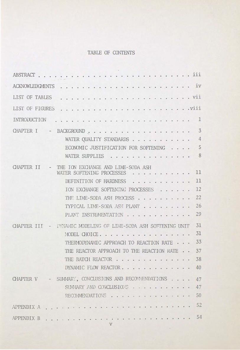
TABLE OF CONTENTS

ABSTRACT • • • . • •

ACKNOWLEDQ.1ENfS

. . 111

. . . . 1 v

LIST OF TABLES .. V1l

LIST OF FIGURES .• V1ll

INTRODUCTION 1

CHAPTER I - BACKGROUND ~ . . . . 3

WATER QUALITI STANDARDS . 4

ECONOMIC JUSTIFICATION FOR SOFTENING 5

WATER SUPPLIES 8

GIAPTER II - TifE ION EXO-IANGE AND LilVfE-SODA ASH WATER SOFTENING PROCESSES . . . . •

DEFINITION OF HARDNESS . . . .

ION EXCHANGE SOFTENING PROCESSES

THE LIME-SODA ASH PROCESS . .

TYPICAL LIME-SODA. ASH PLANf .

PlANT INSTRUMENTATION . . • .

11

. . . . . 11

12

22

26

29

CHAPTER III - :vrJAr.1IC :MODELING OP LIJ\iE-SODA ASH SOFTENING UNIT 31

GIAPTER V

APPENDIX A

APPENDIX B

r~10DEL rnoi CE • • • • • • • • • • • • • • . 31

THERiv10DYNArv1IC APPROAQ-I TO REACTION RATE • 33

THE REACTOR APPROAQ-I TO 1HE REACTION HATE 37

THE BATGI REACTOR . . .• • 38

DYNAMIC FLOW REACTOR . . . . • . . . • . 40

- SUMr·.fl\.R~~ .. -, CONCLUSIONS AND RECOt n'·IRND TIONS

~UMMARY PND CONCLUSIO~,rc

RECOr1MEJ'®ATI01 S

. ,.. . ~ ,.. . . .

v

~ .

. .

. . 47

47

so

52

. . 54

LIST OF REFEREl'JCES . 58

Vl

TABLE

Il-l

II-2

III-1

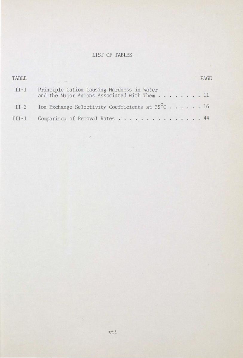
LIST OF TABLES

Principle Cation Causing Hardness in Water and the Major Anions Associated with Them ..

Ion Exchange Selectivity Coefficients at 25°C .

Comparison of Removal Rates . . . . . . . . .

Vll

PAGE

. 11

. 16

. . 44

FIGURE

I-1

II-1

II-2

II-3

II-4

II-5

III-1

III-2

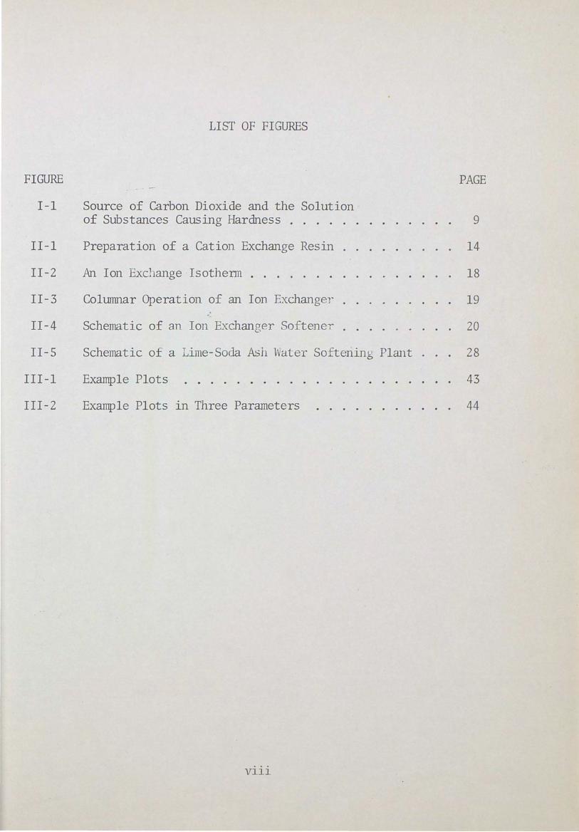
LIST OF FIGURES

So~rce of Carbon Dioxide and the Solution of Substances Causing Hardness .

Preparation of a Cation Exchange Resin

An Ion bxchange Isothenn

Columnar Operation of an Ion Exchanger .

Schematic of an Ion Exchanger SofteneT

Schematic of a Lime-Soda Ash Water Softening Plant .

Example Plots

Example Plots in Three Parameters

Vlll

PAGE

9

14

18

19

20

28

43

44

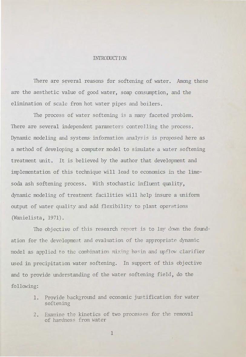
INTRODUCfiON

There are_ ?~veral reasons for softening of water. Among these

are the aesthetic value of good water, soap consumption, and the

elimination of scale from hot water pipes and boilers.

The process of water softening is a many faceted problem.

There are several independent parameters controJling the process.

Dynamic modeling and systems· information analysi~ is proposed here as

a method of developing a computer model to simulate a water softening

treatment unit. It is believed by the author that development and

implementation of this technique will lead to economics in the lime-

soda ash softening process. With stochastic influent quality,

dynamic modeling of treatment facilities will help insure a uniform

output of water quality and add flexibility to plant operations

(Wanielista, 1971).

The objective of this research report is to la) down the found-

ation for the development and evaluation of the appropriate dynamic

model as applied to the comhinatio1 mi::=ing ba~in. and upfJ 01"r clarifier

used in precipitation water softening. In support of this objective

and to provide understandL!g of the water softening field, do the

following:

1. Provide backgromd and economic justification for water softening

2. Examine the kinetics of two processes for t1e removal of hardness fron1 water

1

3. Find theoretical or empirical data or approaches by which the results of the simulation technique may be evaluated.

2

I • BACKGROUND

Two things can be said about water without contradiction. Water

1s the basic fluid of life and without an adequate supply of good water

economic developn1ent will not proceed. The objective of water treatment

is to meet this need. The goal of mllllicipal water t Teatment plants is

to provide water that is potable, chemically and biologically stable,

appetizing and reasonably priced. It is important that these goals be

met so that the consumer will not turn to some other source of water

which is unsafe.

In many parts of the country with the growJng consumption per

capita and growing population i t is increasingly difficult to find a

raw water supply of sufficj ent quanti t ;· and qn::1l i. t·r to meet the public

demand. These corrnnilllities have been fen--ced to tum to water supplies

which are illlfit for consumption in -:-1 E'j T nati VA fonn or t\•ere previolLc;ly

considered unfit for treatment. Many of these new sources are ground

and surface waters either high in color and turbidity, bad tasting, or

hard and staining. Water of high hardness requires softening and

sanitizing to render it fit for consumption.

The requir ements for a public water ~upply are that it:

1. S.t~al} contain no orga.r1j ~J":S \ ;,.L_icj , cau_,P c • .J ~··Pase ..

2. Be c;parkling cJear and colorless_

3. Be good tasting, free from odors, and rreferably cool~

4. Be reasonably ~oft.

3

5. Be neither scale-forming nor corrosive.

6. Be free from objectionable gas, such as hydrogen sulfide, and objectionable minerals, such as iron and manganese.

4

(Riehl, 1962)

Two through six of the above list of requirements indicate the

need for chemical treatment or softening of water. Softening reduces

the soap and detergent consumption and removes the staining character-

istics of water making it more suitable for use in lalllldry and personal

hygiene. Softening can, by removal of fixed dissolved solids, reduce

the accumulation of scale in hot water pipes, water heaters, boilers

and other appliances. Softened water is more acceptable to food pro-

cessing and industrial cooling water requirements. Water high in mag-

nesium and sulfates have l axati.r P. properties. High leYels of sodium

ion concentration may be troubl esome to people on low ?al.t diet.:;.

WATER QUALITY STAl\JDARDS

Standards for water quality have been established by the U.S.

Department of Health, Education, and Welfare for water used on common

carr1ers. The 1962 standards are approved by the American Water Works

Association, 111e Arnei i :::ail Pul,lic Health Association, and t he Water

Pollution Control Federation, and are used hy most state, comty, city,

and connnllllity gover·1ments a th ., criteria for potable water. 111e in-

tent of these ;: ·"-andarcls is -':hat 8 water source consistent.)_·,- n1eet the

standards review below or be treated s o t h At i.t does ..

To meet th r= bacteriological qua.li t ', a water :r;1 y:;t c1nta i~1 no

more than one col·j {· nn c .go _ism in 100 nli of t.an "r~ter.. 2J:;f·ne _ in the i .

standard is the testing frequency. Typical minimillil number of monthly

5

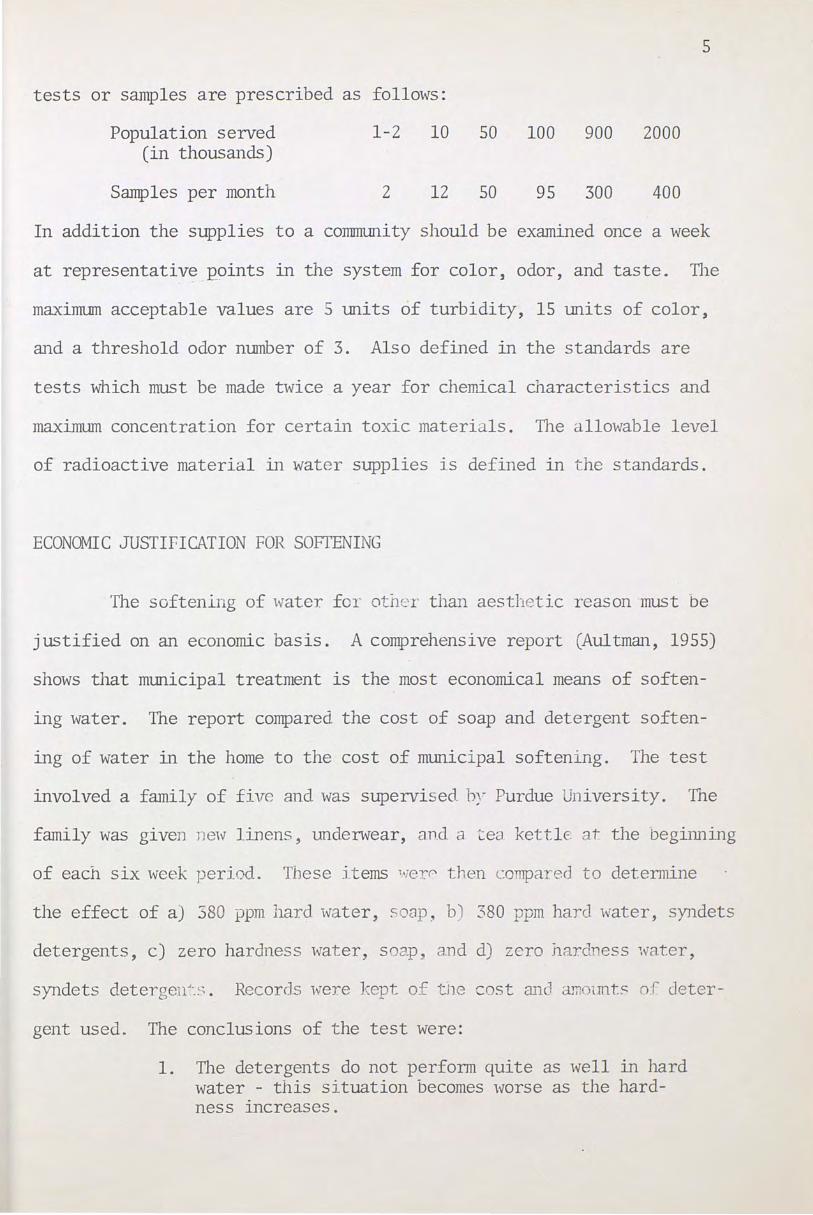
tests or samples are prescribed as follows:

Population served 1-2 10 so 100 900 2000 (in thousands)

Samples per month 2 12 50 95 300 400

In addition the supplies to a community should be examined once a week

at representativ~ _ ~9ints in the system for color, odor, and taste. The

maximum acceptable values are 5 units of turbidity, 15 units of color,

and a threshold odor number of 3. Also defined in the standards are

tests which must be made twice a year for che~~cal characteristics and

maximum concentration for certain toxic materials. The allowable level

of radioactive material n1 water supplies is defined in the standards.

ECONOMITC JUSTIFICATION FOR SOFTENING

The softening of water for other than aesthetic reason must be

justified on an economic basis. A comprehensive report (Aultman, 1955)

shows that mllllicipal treatment is the most economical means of soften-

ing water. The report compared the cost of soap and detergent soften-

ing of water in the home to the cost of municipal softening. The test

involved a family of five and was supervised b/ Purdue University. Tne

family was given ne1v linens, underwear, and a tea kettle at the begi1ming

of each six week peri _.dA These items ~~ier - then compared to detennine

the effect .of a) 380 ppm har¢1 water, soap:t b) 380 ppm hard water, syndets

detergents, c) zero hardness water, soap~ and d) zero hardness 1 rater,

syndets detergeu-'·_~, . Records i ere Jrept of the cost ancl am1 .1mts of deter-

gent used.. The conclusions of the test were:

1. The detergents do not perform quite as well in hard water - this s i tuation becomes 1-vorse as the hard­ness increases.

2. Hardness ions interfere and cause some of the dirt to be redeposited in the fabric.

3. A greater amount of synthetic detergent is needed in hard water.

4. In soft water a 0.15% concentration (of syndets) would clean while in 21 grain hardness, probably 0.3% concentration would be required.

6

It may be assumed·-that softening fairly hard water would save the aver-

age family 1/3 to 1/2 carton of detergent (20-22 oz. size) per week.

To bring the cost data to 1970 dollars the ratio of the con-

sumers' retail index was used (World Alrnru1ac, 1971). Soft water could

save $48.00 per year for a family of five for syndets detergents and

$74.38 per year for soap exclusively. Assuming present day usage of

predominately detergents this means a $9 .76 savings per person per year

in zero hardness water. The $9 . 76 savj11gs reduces to $7 ~ 36 for 100 ppm

hardness water. It was calculated (Aultman, 1955) that t he municipal

plant could produce water of 100 ppm hardness for a treatment cost of

$1.83 per person per year. The net savings per person per year for

municipally softened water versus detergent softened water is $5.53 per

person per year. "Thus for each $1 spent at the pJant $4 is saved in

the home" (Riehl, 1962). This is a great benefit to the underprivileged

who can not afford to soften their own water an~~ay except by deter-

gents. Softening also helps reduce the amoliDt of detergents that are

difficult to degrade; thus, the amounts of pollution bein ~ dumped into

our natural water.~ are decreasecL .f\ul tD:4n also indicated t ,e fo llowj ng

additional benefits resulting in savings due to softened water.

1. A 25% savings is realized on fuel for heating soft water by the elimination of deposits of scale which retards heat flow.

2.

3.

4.

5.

6.

An 18% savings is obtained on repa1rmg, cleaning, and replaci!lg plumb~g that is caked. ·

Fabrics show 25% less wear and tear in soft water.

Food cooked in soft water retains its natural color and appearance, and its digestive properties.

In making tea and coffee, 50% less leaves and _grounds are used in soft than in hard water.

Soft water provides for better skin care, and eliminates the need for expensive bubble bath pre­parations. There is no bathtub ring.

Another method of water softening i s the home softener or ion

exchange colliDU1. Based on prices and usage information obtained from

the Culligan Water Conditioning of Orange County, Inc. and -Montgomery

7

Ward Mail Order Catalog, and estimate of home water softening cost was

obtained. These calculations are given in Appendix A. The calculations

were made by reducing 380 ppm hardness to 100 ppm hardness in order to

compare with the milllic.ipal softening costs. The capital and operating

cost of a softener maintained to produce 100 ppm of soft water over a

10 year service life period is $12.03 per person per year . The rental

of a Culligan softening tank, i nstalled and maintained by the company

cost $43.60 per person per year. When compared to the $1 .. 83 per person

per year for municipal softening the advantage is readily seen. ·

Softening has the following advantages from the plant operation

standpoint. When the softening of surface waters accompanies the re-

moval of turbidity and color, the added precipitates due t o softening

accelerate the sedin1entation process. When magnesium i s precipi tated

as magnesium hydroxide, the gel at inous precipitate acts as a coagulant

aid. Softening also reduces the l oad on t he f ilters anc. .1 cncrthens t he

period between backwash, thus reduci!lg the costs associated with t he

filtration (Riehl~ 1962).

8

WATER SUPPLIES

Raw water supplies ar~ generally to two types: surface water or

ground water. Surface water is generally turbid, colored, high in

organ1srns and organic material and medium to low li1 mineralization or

hardness. The degree of mineralization changes with the seasons, low

stream flow being the most mineralized.

These surface waters are generally treated with aluminum and

1ron sulfates as coagulant aids to remove turbidity and color by

flocculation and sedimentation. Surface waters are sometimes bad

tasting and have an illlpleasant odor. This is primarily due to the

organic mater1al~ either alive or dead, in the water. Surface waters

are often polluted from man-made sources. In spite of these drawbacks,

surface waters are the ones most used by large cities. For example,

'in Ohio _, in 1961, there were 538 public water supplies serving approxi­

mately 7 million people (1960 census). Of these public ~upplies 80%

were well supplies, but the 20% which were surface water supplies

served 72% of the people (Riehl, 1962).

Ground waters are generally low 1n turbidity, color, organ1c

matter, and organisms, but are more highly mineralized than surface

waters. Gro1.ll1d water comes from infiltrated rain. Rainwater as it

falls upon the earth is incapable of dissolving the tremendous amo1.ll1ts

of solids foliD.cl in groood waters. The rain water absorbs co2 from

bacteria in the top soil forming carbonic acid. (H2co3). i'.~ the rain

water infiltratE-~s jnto the earth, it is this acia whic1 dissolves cal­

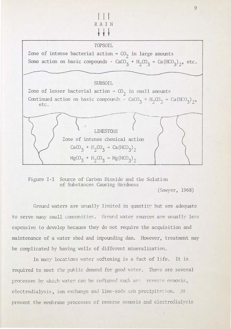
ciwn and magnesitm salts to produce hardnes~ jn grn mc1 ,-a1-P " as indicated

in Figure I-1.

9

r I I RAIN

~ i l TOPSOIL

Zone of intense bacterial action + co2 1n large amounts

Some action on basic compounds - Caco3 + H2co3 + Ca(HC0

3)

2, etc.

SUBSOIL Zone of lesser bacterial action ~).. co

2 ln small amolllts

Continued action on basic compounds - Caco3 + H2co3 + Ca(HC03) 2, etc.

.· Lil\1ESTONE

Zone of intense chemical action

CaC03 + H2co3 + Ca(HC03) 2

MgC03 + H2co3 + Mg(HC03) 2

Figure I-1 Source of Carbon Dioxide and the Solution of Substances Causing Hardness

(Sawyer, 1968)

GroLnld waters are usually limited in quantity but are adequate

to serve many small communities. Gro1.md water sources are usually less

expensive to develop because they do not require the acquisition and

maintenance of a water shed and impol.lllding dam. However, treatment may

be complicated by having wells of different mineralization.

In many locations water softening is a fact of life. It is

required to meet the public demand fo~ good K8.ter. There are several

processes by ·vv·hich water can be softened such as· re"' er~e nsmosis,

electrodialysis, ion exchange and lime-soda ?..sh precipit~ -r-- · on . At

present the membrane processes of reverse osmosis and electrodialysis

10

are too e:xpens1ve except where h.igh concentration of dissolved solids

must be removed because of limited choice of supply. Ion exchange has

widespread use but is limited by cost to smaller applications. Lime-

soda ash process is the least expensive when applied to municipal treat-

ment and has the following advant.ages (Riehl, 1962):

1. - Disinfection

2. Removal of organic material and bacteria

3. Eliminates worry about well contamination

4. Simultaneous removal of iron and manganese with hardness

5. Aids coagulation and flocculation of turbid water

6. Controls turbidity and aids filtr0tion

There are more than 600 lime-soda ash installations 1n the

United States and several jn Florida. Because of tbe frequency of its

use and the advantages listed above, the detailed evaluation of the

lime-soda ash process is warranted.

II. TilE ION EXCHANGE AND LIME-SODA ASH

WATER SOFTENING PROCESSES

DEFINITION OF HARDNESS

To the conslUiler hard water is water that requ1res large arnomts

of soap to form a lather. With hard water, scale is formed in appliances,

hot water pipes and boilers. This condition is brought about by concen­

trations of dissovled divaleht metallic cations and the anions they

associate with in natural waters. When water is heated some of these

mineral compounds decrease in solubility and precipitate out in pipes

and boilers forming scale. In addition, the divalent ion~ combine with

soaps and to a lesser extent detergents, to form precipitates. The

precipitates are partly the cause of bath tube rings and make cleaning

and washing clothes more difficul·t. The divalent metallic cations

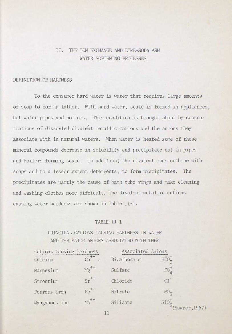
causing water hardness are shown in Table II -1.

TABLE II-1

PRINCIPAL CATIONS CAUSING HARDNESS IN WATER

AND THE MAJOR ANIONS ASSOCIATED Willi THEM

Cations Causing Hardness

Ca++

Calcium

MagnesiliDl Mg++

Strontium Sr++

Ferrous iron Fe++

:Manganous ion :Mn.++

11

Associated An.ions

Bicarbonate HC03

Sulfate

Chloride

Nitrate

Silicate

c::nJ-~ 4

C.l

li03

sio: :J(Sawyer,l967)

12

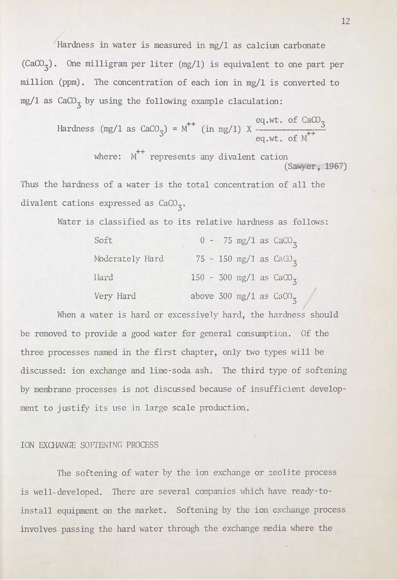
i Hardness in water is measured in mg/1 as calcium carbonate

(CaC03). One milligram per liter (mg/1) is equivalent to one part per

million (ppm). The concentration of each ion in mg/1 is converted to

mg/1 as Caco3 by using the following example claculation:

++ Hardness _(mg/1 as CaC03

) = M eq.wt. of Caco3 (in mg/1) X ------

of M++ eq.wt.

where: ++ M represents any divalent cation (~YlJl=er, 1967)

Thus the hardness of a water is the total concentration of all the

divalent cations expressed as Caco3.

Water 1s classified -as to its relative hardness as follows:

Soft 0 - 75 mg/1 as Caco3 l\'Ioderately Hard 75 - 150 mg/1 as Caco3

liard 150 - 300 mg/1 as CaC03

Very Hard above 300 mg/1 as Caco3 I When a water is hard or excessively hard, the hardness should

be removed to provide a good water for general consumption . Of the

three processes named in the first chapter, only two types will be

discussed: ion exchange and lime-soda ash. The third type of softening

by membrane processes is not discussed because of insufficient develop-

ment to justify its t~e in large scale production.

ION EXCHANGE SOFTENING PROCESS

The softening of water by the 1on exchange or zeolite process

1s well-developed. There are several companies which have ready-to­

install equipment on the market. Softening by the ion exchange process

involves passing the hard water through the exchange media where the

13

unwanted divalent cation is absorbed and the water is softened. When

the exchanger media is saturated with hardness ions, it is regenerated

with a salt (NaCl) solution.

A number of natural materials have ion exchange ability includ-

1ng soils, humus, cellulose, wool, protein, activated carbon, coal,

lignin, metallic oxides, and living cells such as algae and bacteria.

Reviews of ancient Greek literature indicate the use of clays and min-

erals for demineralizing drinking water. In 1876 Lernbury demonstrated

reversible ion exchange reactions in transforming the mineral leucite

(K2oAI2o3 · 4Si02) to m1alcite (Na20A12o3 · 4Si02) and back (Weber,

1972). The original application of zeolites to softening is credited

to Gans, a German chemist who called the process pennutits (Riehl, 1962).

In 1935, a modern resin exchanger was discovered by I. B. A. Adams and

E. L. Holmes. The media was crushed, phenolic phonograph records

(Weber, 1972).

The zeolite 1s natural r1ver sand commonly called green sand.

These are natural aluminosilicates (Al2o3 · 4Si02) and exchange sodium

(Na+) for calcl·um (Ca++). A h · J. ,_ d b d · synt et1c zeo.1te canoe rna e y rylng

mixed solutions of sodium silicate (Na2Si03) and sodiwn aluminate

(Na2Al

2o

3). These are then crushed to the desired size. All zeolites

operate on the sodium cycle and are regenerated with salt solution

(Fair, 1968).

At the present, synthetic ion exchange resms are the most fre­

quently used exchange material. Depending on the choice of resin these

resins can exchange anions or cations. Synthetic resins have the cap-

ability to exchange on a selective basis. Some resins cal be regen­

erated on moTe than one jon cycle. In softening res1ns, t o types

14

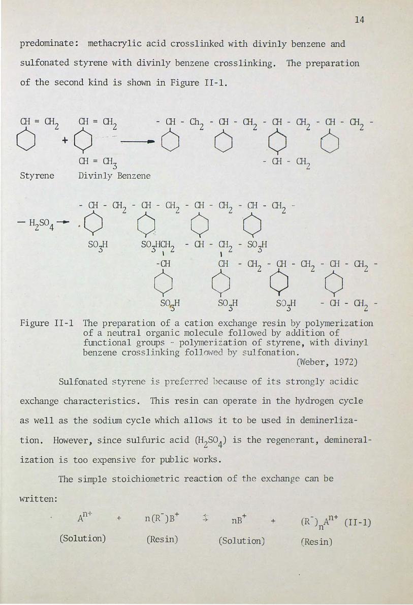
predominate: methacrylic acid crosslinked with divinly benzene and

sulfonated styrene with divinly benzene crosslink0g. The preparation

of the second kind is shown in Figure II-1.

- CH - Q-12 -

6 Styrene

- rn - Q-12 - rn - CH - rn - rn2 - CH - rn -

·0 c) 2

0 ·o 2 - H SO --+-

2 4

S03H S03HCH2 - rn - rn2 - SO H

' ' 3

-rn CH -rn 2 -o- rn2 - rn - rn-2

0 0 0 S0

3H S03H SO H 3 -rn-rn-2

Figure II-1 The preparation of a cation exchange resin by polymerization of a neutral organic molecule followed by addition of functional groups - polymerization of styrene, with divinyl benzene crosslinking foll0wecl by sulfonation .

(Weber, 1972)

Sulfonated styrene i s preferr ed )ecause of its strongly acidic

exchange characteristics. This resin can operate in the hydrogen cycle

as well as the sodium cycle which allows it to be used in deminerliza-

tion. However, since sulfuric acid (H2so4) is the regenerant, demineral­

ization is too expensive for public works.

written:

The simple stoichiometric reaction of t he exchange can be

n+ A

(Solution)

+ ~-·

-+ + nB

(Solution)

+

(Resin)

15

However, this is not quite true s1nce 1on exchange is a sorption

phenomenon rather than a reaction. However, it does provide a good ana­

lytical model. An+ is a multivalent ion, B+ 1s a monovalent ion and R

represents the res1n.

Synthetic resin demonstrates a distinct selectivity in the rate

of sorption of ions. If several ions are present in the same concen-

tration, one may be removed much faster than the rest. This affinity

for different ions by the resin can be expressed in a series . A typical

example is:

Li++ + + + + + + 1. < H < Na < K = NH4 < Rb < Ag

2. Mg++ ++ Cu++ ++ ++ ++ ++ = Zn < < Co < Ca < Sr < Ba

(Fair, 1968)

This characteristic of resins 1s quantified by the selectivity coef­

A. ficient, KB.

~ =

[B+]n (X RnA) (£RnA) (II-2)

[An+] n n (XRB) (fRB)

Where: [ ] = denotes molar concentration

X = equivalent ionic fractions

f = activity coefficients

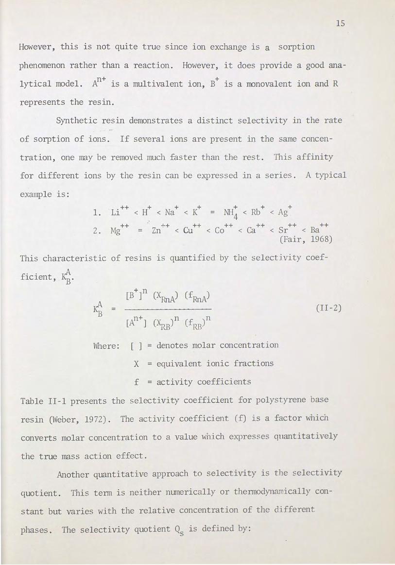
Table Il-l presents the selectivity coefficient for polystyrene base

resin (Weber, 1972). The activity coefficient (f) is a factor which

converts molar concentration to a value which expresses quantitatively

the true mass action effect.

Another quantitative approach to selectivity is the selectivity

quotient. This term is neither numerically or thermodynamically con­

stant but varies with the relative concentration of the different

phases. The selectivity quotient Q is defined by: s

16

TABLE II-2

ION EXCHANGE SELECTIVITY COEFFICIENTS AT 25°

Replaceable Ion Cross linking

4% 8% 16%

Monovalent cations - ·

Li 1.00 1.0 1.0 H 1.32 1. 27 1.47 Na 1.58 1.98 2.37 K 2.27 2.90 4.50 Rb 2.46 3.16 4.62 Cs 2.67 3. 25 4.66 Ag 4. 73 8.51 22. 9 Tl 6.71 12.4 28.5

Divalent cations

Mg 2.95 3.29 3.51 Ca 4.15 5.16 7.27 Sr 4.70 6.51 10.1 Ba 7.47 11.5 20.8 Pb 6.56 9.91 18.0

Monovalent an1ons (2% c.1.)

OH 0.80 0.50 F 0.08 Cl 1.0 1.0 Br 2.7 3.5 I 9.0 18.5 N03

-~ . 0

SCN 6.0 4.3 ClO 9.0 10.0

Data are for polystyrene base resins, sulfonic acid cation exchanger, and type 2 quarternary base anion exchanger. Data of Boooer and Smith (J. Phys. Chern., 61, 326) for cation exchanges; Gregor, Belle, and Marcus (J. Arner, Chern. Soc., 77, 2731) for anion exchanges .

A value greater than 1 indicates preferential absorption of ion named against the reference ion (Li for cations, Cl for anions).

Source: L. ~1ei tes , Handbook of An alytica1 wemis try ·' Mc(;r;:u..., -Hill Book Company, New York, 1963.

(Weber, 19 72)

17

[~A] [B+] QMoles .An+ ./ gm .resin) QMoles B+/ml solution)

Qs == ......... [RB-----]--[A_n_+_] = ·n ,if 1 B+ I . ) rr-. n+/ . vvJ.O es gm resn1 v'1oles A ml solut1on)

If Qs == 1, the resin shows no selectivity. For Qs > 1, the resin has a

preference for An+ and if Q < 1, it has a preference forB+. The s

larger the value of Qs the shorter the le.ngth of ion exchange colliDlll

required (Weber, 1972).

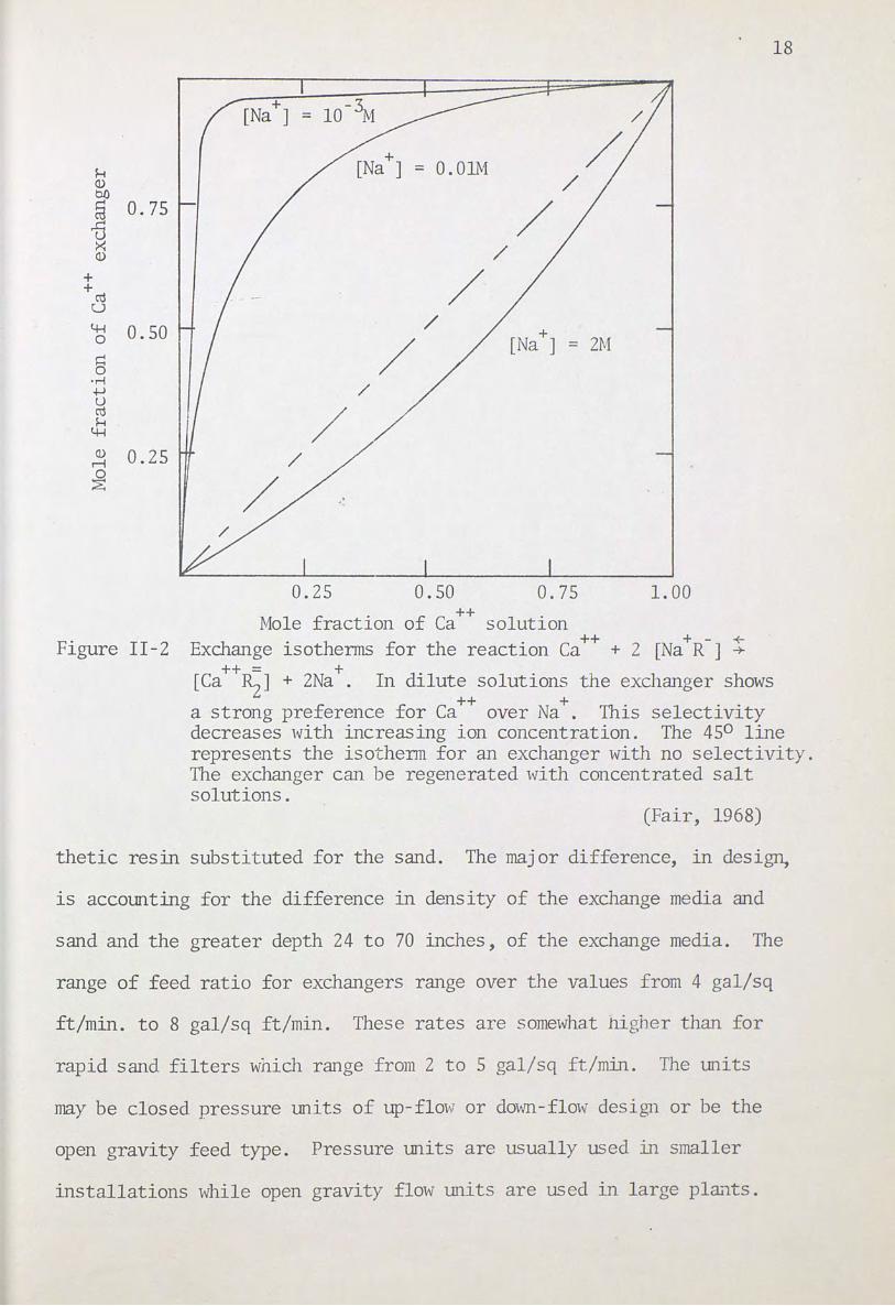
From the above discussions~ the distribution of two ions of

different valence between the solution and resin is strongly dependent

on solution concentrations. In hetero-ionic exchange, the resin

increasingly prefers the divalent ion to the monovalent ion with de-

creasing concentrations in the solution. The equilibrium position can

be characterized graphically by the exchange i sotherm of Pigure II-2.

For no selectivity, the line is the dia:;onal of t he grapJ . The curves

above the diagonal show preference for Ca++ and curves below the diagonal

show preference for Na+ (Fair, 1968).

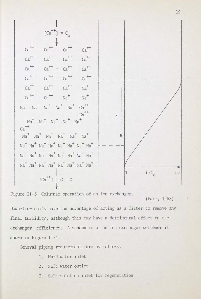
The quality of operation of an 1on exchange column is represented

by the breakthrough curve. This curve 1s obtained for each installation

and shows the capacity and quality of the column. Figure II-3 shows

this type of curve and a schematic of an exchange column or bed . The

flatter the line the better the efficienc. ' of the colllllm. TI1e degree of

tailing in the breakthrough curve gives an indication of channeling of

flow or foulin g of the exchange material . The point at '"'hich t he ion

being removed appears in t he effluent · c:: called the hreakthrough point.

It indicates the end of an exchange cycle and calls for the regeneration

of the column (Fair, 1968).

A typical ion exchange softener installation usu~l ly cons i sts of

one or more units similar to mechanical filt er s with zeolite or syn-

18

H = O.OIM ~ ~

§ 0.75 ~ ~ / ~

+ / + ro u LH 0.50 /

[Na+] 0

/ = ~ ~ 0

'M ~ / u ro / H

LH ~ 0.25 ~ 0 ~

> -

0.25 0.50 0.75 1.00

Mole fraction of Ca++ solution Figure II-2 Exchange isotherms for the reaction Ca++ + 2 [Na+R-] ~

++ = + [Ca RzJ + 2Na . In dilute solutions the exchanger shows

a strong preference for Ca++ over Na+. This selectivity decreases with increasing ion concentration. The 45° line represents the isotherm for an exchanger with no selectivity. The exchanger can be regenerated with concentrated salt solutions.

(Fair, 1968)

thetic resin substituted for the sand. The major difference, in desi~

is accounting for the difference in density of the exchange media and

sand and the greater depth 24 to 70 inches, of the exchange media. The

range of feed ratio for exchangers range over the values from 4 gal/sq

ft/min. to 8 gal/sq ft/min. These rates are somewhat nigher than for

rapid sand filters which range from 2 to 5 gal/sq ft/min. The units

may be closed pressure units of up-flow or down-flow desi~1 or be the

open gravity feed type. Pressure units are usually used in smaller

installations while open gravity flow units are used in large pl&its.

[Ca++] = c 0

~ Ca++ Ca++ Ca++ Ca++

Ca++ Ca++ Ca++ Ca++

Ca++ ++ Ca -··- Ca++ Ca++

Ca++ Ca++ Ca++ Ca++

Ca++ Ca++ Ca++ Na+

Ca++ Ca++ Na+ Na+

Na + Na+ Na+ Na+ Na+ Ca++

c ++ -· a X

Na+ Na+ Na+ Na+ Na+ Ca++

Na+ Na+ Na+ Na+ Na+ Na+

Na+ Na+ Na+ Na+ Na+ Na+ Na+ Na+

Na+ + + + Na Na Na Na+ Na+ Na+ Na+

Na+ Na+ Na+ Na+ Na+ Na+ Na+ Na+

I 0

[Ca++] = c = 0

~ Figure II-3 Columnar operation of an lOll exchanger.

C/C 0

(Fair, 1968)

19

1.

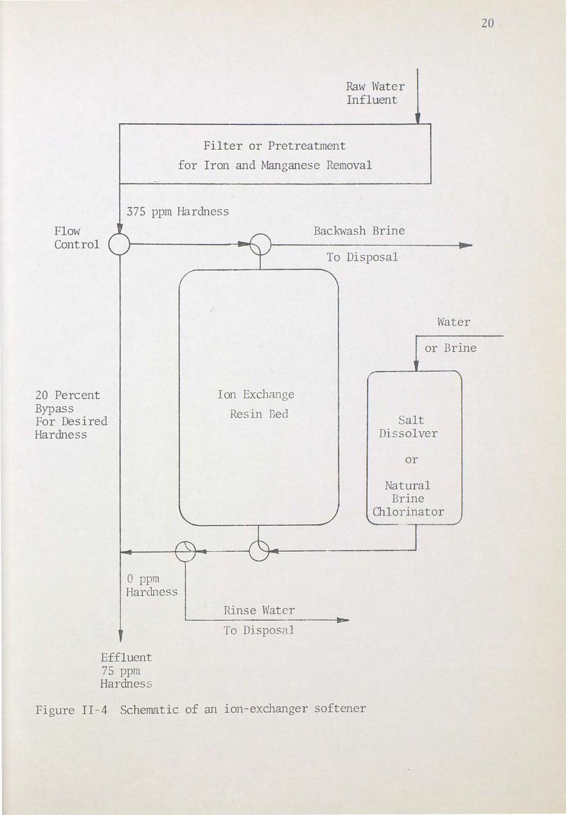
Down-flow units have the advantage of acting as a filter to remove any

final turbidity, although this may have a detrimental effect on the

exchanger efficiency. A schematic of an ion exchanger softener is

shown in Figure II-4.

General piping requirements are as follows:

1. Hard water inlet

2. Soft water outlet

3. Salt-solution inlet for regeneration

Filter or Pretreatment

Raw Water Influent

for Iron and Manganese Removal

375 ppm Hardness

Flow Control

20 Percent Bypass For Desired Hardness

0 ppm Hardness

Effluent 75 ppm Hardnes.;J

Ion Exchange

Resin Bed

Rinse Water

To DisposaJ

Backwash Brine

To Disposal

Water

or Brine

Salt Dissolver

or

Natural Brine

. Chlorinator

Figure II-4 Schematic of an ion-exchanger softener

20

4. Combination salt-solution, rlnse, and backwash water outlet

5. Wash water or backwash inlet usually used to back­wash when exchanger is used as filter

6. Controls for flow rates

7. Sampling cocks on soft water outlet, wash water _o_u.tlet and salt solution inlet

8. Typical mder drainage system or support for exchange media

21

Three important economic considerations in ion exchange soften-

ing design are the availability and cost of salt, problems of brine

disposal and tha amolffit of iron in the water. Iron when in its tri-

valent state is easily oxidized to form an iron oxide collodial sus-

pens1on. This suspension can clog the pores of the exchange media and

gradually reduce its effectiveness to zero. Thus iron-bearing water

must be pretreated to remove the trivalent iron, thus increasing the

operating and physical costs of the softening facility (Riehl, 1962).

The cost of salt varies from place to place. If natural brine

waters are available their concentration should be considered in the

cost analysis because they are generally not as effective as prepared

solutj ons. Sea water may be used but must be disinfected first. The

disposal of the wasted brine is a diffj cult problem. If disposed of

jn a surface water, sufficient dillution must occur to avoid polluting

the water and kj!ling marine life. The brine can also be disposed of

by deep well injection but care must be taken not to pol1l 1te fresh

water aquafiers.

22

THE LIME-SODA ASH PROCESS

In the lime-soda ash softening process, unwanted hardness ions

are removed by precipitation rather than by substitution as in the ion

exchange softening process. The process has several advant.ages, such

as disinfection, - reduction in dissolved solids, and simultaneous

removal of iron and manganese with hardness.

Cavendish of England is credited with discovering softening by

lime ln 1766. He added lime to natural water and deposited the carbon-

ates of calcium (CaC03) and magnesium (]'.1gC03) . Dr. Thomas Clark of

Aberdeen, Scotland built the first large scale plant lll 1841. In 1856,

Dr. Porter, of London, suggested the use of soda ash to remove non-

carbonate hardness.

The first municipal 1~ater softening plant in the United States

was built in Oberlin, Ohio and there are presently over 600 municipal

plants in the United States using lime or l ime-sod.'1 ash softening

(lhehl, 1-962). ""~ j Softening 1 y the lime-soda ash process removes the diva] ent

alkyline earth cation by precipitation. The major contributors to

. . ( ++) d . c·u ++) hardness m natural waters are calc1um · Ca an magnes1um 1v1g .

For this reason the lime-soda ash process 1s based on t~eir precipi-

tation.

Calcium associates itself with the rri r J.ous an1on · J is ted lll I

Table II -1. Calcium has a hypothet i -:P..1. a.ff~_n j t _. fry~~ ea r:1 of thf'

different anions. J ,is ted in d creasing order of a££ini -1:'- . caJ c ·l rrn

forms these compounds, calcium bicarbonate (Ca(HC03) 2), calcilllll sulfate

(Caso4), calcium chloride (CaC12), calcium nitrate (Ca(N0~) 2), and

23

calcimn silicate (CaSi03) (Riehl- - 1962). Depending on the individual

water supply some or all of these may be present. Compomds containing

the bicarbonate (Hco;) and the carbonate ceo;) radical are classed as

carbonate hardness. Sulfate (S04J, chloride (Cl-), n_itrate (N03), and

silicate (Si03J are classed as non-carbonate hardness. Carbonate hard­

ness 1s removed -by calcium hydroxide (Ca(OH)2), hydrated lime. Suf-

' ficient calcium hydroxide is added to raise the pH to 10.8 (Sawyer,

~). This convert~ the bicarbonate form to the carbonate form

simultaneously exceeding the solubility of calcium carbonate and precip-

ating it from solution. This 1s described by the following equation: .·

pH 10.8

However 17 mg/1 as Caco3 will remain in solution due to the slight solu­

blity of CaC07 • J

The non-carl onate hardness of c.tlciurn is renoved by precipitating

it with sodium carbonate, (Na2co3), soda ash. The following reactions

describe the precipitation of calcium non-carbonate hardness.

Ca~t)4 + Na2co3 -+ CaC03 + + Na2so4 (II - 4)

(II- 5)

(II-6)

(II -7)

Magnesium is the second most abliDclant hardnPss -caus ing cation.

Like calcium, it has different hypothetical affinity for the different

anions in Table . T-1. In order of decrca_sing affinity _ magnesi1..un forms

the following compc.mds such as: magnesium bicarbonate (I"1g(HC03) 2),

magnesium. sulfate (MgSO 4), magnesium cloride O!tgC12), magr.esiwn nitrate

24

QMg(N03)

2), magnesium silicate O~Si03) (Riehl, 1962). Magnesium

hardness is removed by precipitation as magnesium hydroxide (Mg(OH)2)

at an optimtun pH of 10.8 (Sawye:, l-967). Calcium hydroxide is used to

raise the pH and provide the hydroxly ions, (OH-).

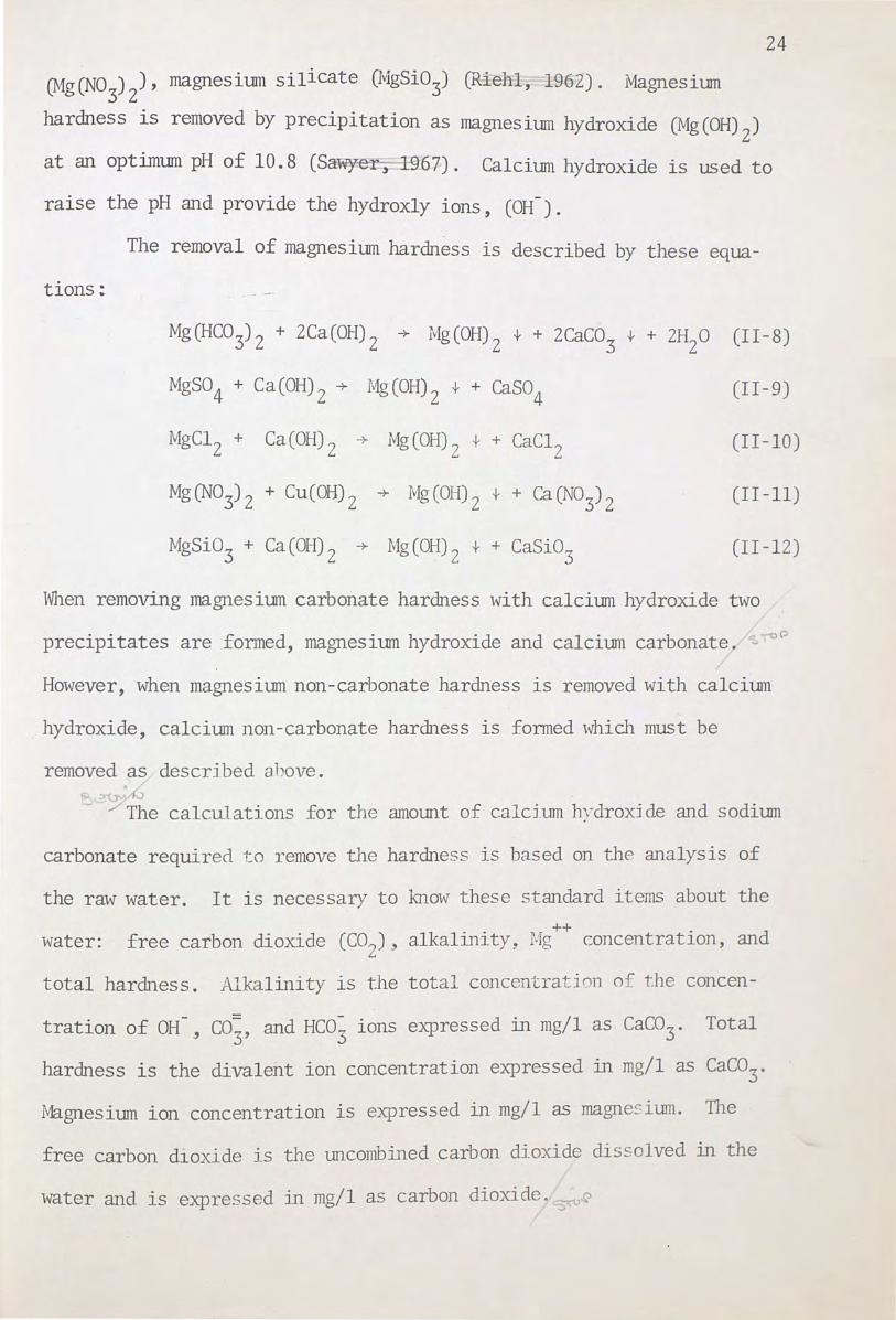
The removal of magnesium hardness is described by these equa-

tions:

Mg(HC03) 2 + 2Ca(OH) 2 -+ :Mg(OH) 2 + + 2Caco3

+ + 2H2o (II-8)

MgS04 + Ca(OH) 2 -+ Mg(OH) 2 + + Caso4

(II-9)

MgC12 + Ca(OH) 2 -+ Mg(OH) 2 + + CaC12 (II-10)

Mg(N03) 2 + Cu(OH) 2 -+ Mg(OH) 2 + + Ca(N03) 2 (II-11)

MgSi03 + Ca(OH) 2 -+ Mg(OH) 2 + + CaSi03 (II-12)

When removing magnesium carbonate hardness with calcium hydroxide two

precipitates are formed, magnesium hydroxide and calcium carbonate. ~~

However, when magnesium non-carbonate hardness is removed with calcium

hydroxide, calcium non-carbonate hardness is formed which must be

removed as descrjbed a1ove. 1)

./ The calculations for the amollllt of calcium hy·droxj de and sodium

carbonate required ~o remove the hardness is based on the analysis of

the raw water. It is necessary to know these standard items about the

water: free carbon dioxide (C02), alkalinity, lfg ++ concentration, and

total hardness. Alkalinity is the total conccntratjon of the concen­

tration of OH-, co;, and Hco; ions expressed in mg/1 as CaC03. Total

hardness is the divalent ion concentration expressed in mg/1 as Caco3.

Ma.gnesitun ion concentration is expressed in mg/1 as magne ium. The

free carbon dioxide is the uncombined carbon dioxide dissolved in the

water and is expressed in mg/1 as carbon dioxide. ~~

25

If the total hardness is greater than the alkalinity, the non­

carbonate hardness is the difference between the two. If the alkalinity

is greater than the total hardness there is no non-carbonate hardness.

Excess lime is the amount used to raise the pH and supersaturate the

solution to speed precipitation. Excess lime treatment may be eliminated

when a water contairis less than 40 mg/1 as Caco3 magnesium hardness

(A.W.W.A., 1969). Excess lime is a matter of economic importance and

1s different for each individual raw water .

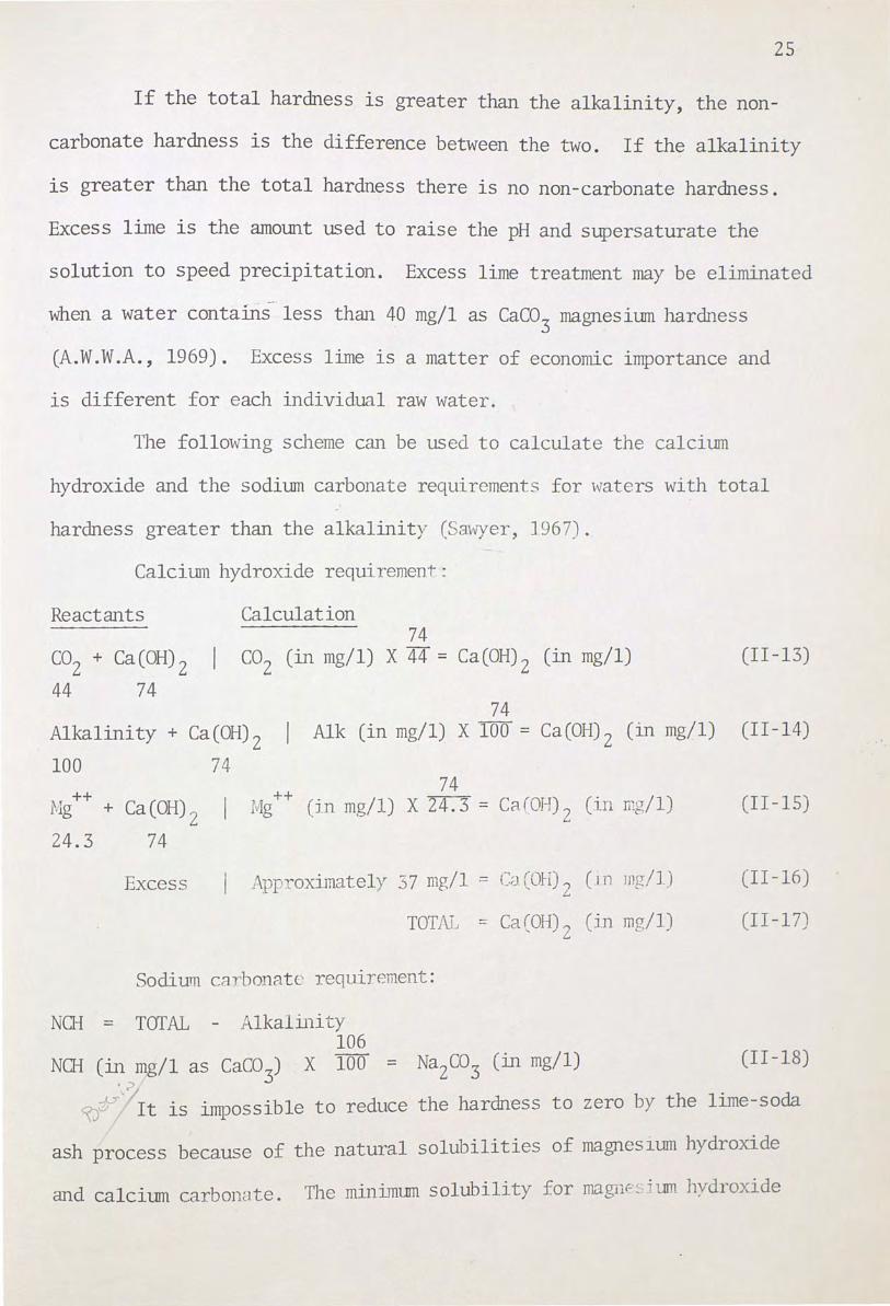
The following scheme can be used to calculate the calcium

hydroxide and the sodium carbonate requi r ements for \~aters with total

hardness greater than the alkalinity (Sawyer , 1967) .

Calcium hydroxide requirement:

Reactants Calculation 74

C02 + Ca(OH) 2 C02 (in mg/1) X 44 = Ca(OH) 2 (in mg/1) (II-13)

44 74 74

Alkalinity + Ca(OH) 2 Alk (in mg/1) X 100 = Ca(OH) 2 (in mg/1) (II-14)

100 74 ++

}.'lg + Ca (OH) 2

24.3 74

Excess

74 1·.tlg ++ (in mg/ 1) X 24.3 = Ca(OH) 2 (i n n:f/1)

App --oximately 37 mg/ 1 = Cr . (01-i) 2 (.1 n mg/1.)

TOTAJJ == Ca (0H) 2 (in mg/1)

Sodium ca rbonatt r equir(ment :

NOH = TOTAL - Alkalli1it y 106

(II -15)

(II - 16)

(I I -17)

NOH (in mg/1 as caco3) X 100 = Na2co3 (in mg/1) (11-18)

•;>

t:Qy It is impossible to reduce the hardness to zero by the lime-soda

ash process because of the natural solubilities of magnesium hydroxide

and calcium carbonate. The minimum solubility f or mag111~ ~- jum hydroxide

26

is about 9 mg/1 and about 17 mg/1 for calcium carbonate. For this

reason it is not possible to produce water of hardness less than 25 mg/1.

In addition, both magnesium hydroxide and calcium carbonate tend to

form supersaturate.d solutions that do not approach saturation rapidly

even in the presence of precipitated material. In practice it is -

uneconomical to allow sufficient detention time for complete precipit-

ation or complete settling of precipitated material already formed. So

from practical consideration, waters softened by the lime-soda ash

process usually have a residual hardness between 50 and 80 mg/1 as

caco3 (Sawyer, 1967). ~ '

Dissolved solids should not be confused with hardness. A water

can be low in hardness yet high in dissolved solids. For example, a

salt (NaCl) solution could have 1000 mg of salt dissolved in one liter

of water. The example solution has zero l1ardness because no divalent

cations are present but has 1000 mg/1 dissolved solids. This is an

important plus for the lime-soda ash softeninB proce'S as compared to

the sodiwn cycle jon exchange softening. For example, for every pomd

of lime (CaO) added to water hard with calcium carbonate hardness, 3.5

pounds of precipitate is fanned This same pomd of lime removed 2. 9

pounds of hardness. This shows dramatically the amomt o£ dissolved

solids removed, but it also points out one of the problems associated

1·vith lime-soda ash process: the amount of s ud ,e generated by this

process crea.tes quj te a large d · sposal prob.~ eJil ...

TYPICAL LirviE-SODA ASH PLANI'

A typical modem installation csing t1 e _ ime - soci:'~ a~h p~oc ~s

1s the Claude H. ~Tal Water Treatment Plant at Cocoa, Florida. The

27

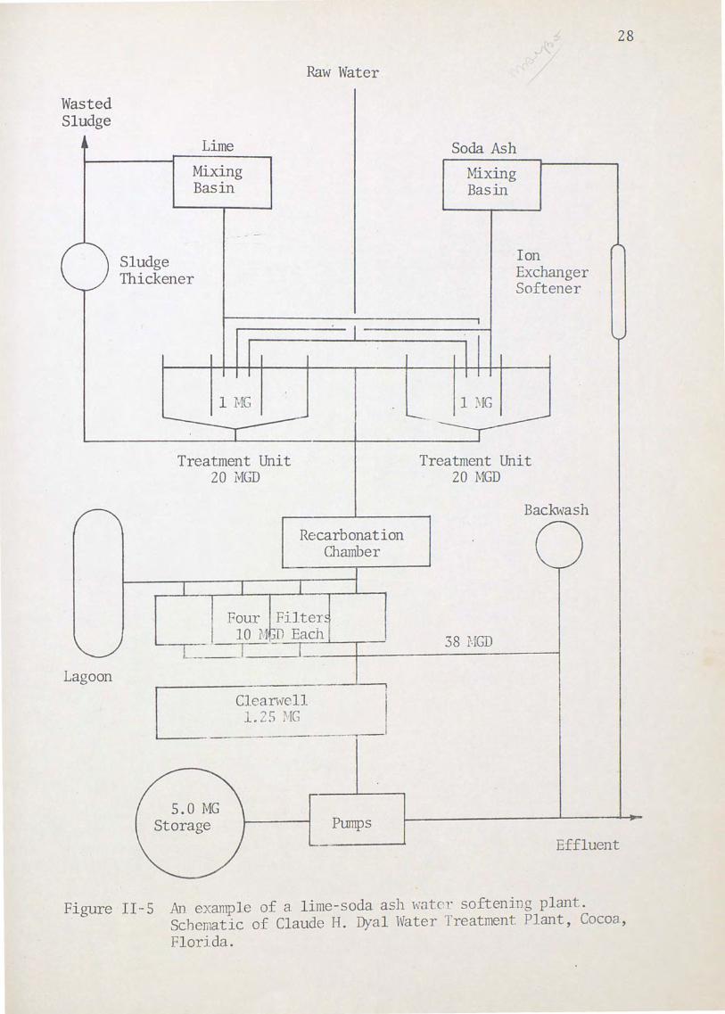
plant softens a gromd water of 3~5 !fig/l_hardness (as Caco3) to 85 mg/1

effluent hardness. The plant has a capacity. of 40 J4GD. The plant con­

sists of two 1 MG Eimco Treatment Units, two chemical mixing basins, a

recarbonation basin and four filters of 10 MGD each.

The most important part of the complete treatment process 1s

the Eimco Treatment Unit:· The treatment unit is an up-flow clarifier

with a rapid mixing well in the center. The sludge rakes and rapid

mixing turbines rpm may be varied from 5. 5 to 7. 5 rpm. The maximum

flow is 24 MGD giving the llllit a one hour detention time.

The chemicals are fed into the center mixing well ln the

clarifier where they are mixed with the raw water. The lime and soda

ash are delivered in the fonn of water solutions or suspensions.

Potato starch, used as a coagulant aid, is injected into the raw water

just prior to the raw water entering the mixing well.

The milk of lime solution is prepared in the lime mixing basin.

The lime is fed into the basin by two shakers. In the basin it is

mixed with sludge water from the sludge thickener by two mixers. The

system is capable of supplying over 3000 poliDds per hour of m1slaked

lime. From the lime mixing bas in overflow, the suspended solution of

lime is pwnped on demand to the cl arifier. The plmlping rate is con-

trolled automatjcally to supply sufficient lime to keep the pH in the

mixing well at 10.1.

The soda ash solution is prepared jn a basin similar to the lime.

Water with zero hardness is used to dissolve the soda as11. It comes

from the plant effluent and is softened by ion exchange. The equipment

is capable of preparing over 1200 pomds per hour of dry soda ash. The

overflow from the soda ash mixn1g basin is pumped automa~ically to the

Wasted Sludge

~

Lagoon

Lime

Mixing Basin

- -- -

Sludge Thickener

1 MG

T

Treatment Unit 20 Iv1GD

I

Raw Water

I

Recarbonation Chamber

J

Soda Ash

Mixing Basin

Ion Exchanger Softener

I

1 ~JG

Treatment Unit 20 MGD

Backwash

28

..... ~

,,....

Four Filter-~ 10 d ,SD Each

l ____ l -=y-__ ~-~~~~~-~------3_8_r_-~_D ______ ~

D~an-vell j '· .. 2 S l'IG ___ __ " _ ___,._ I

-5.0 MG

I Storage \ I Pumps

L.--------..

Effluent

Figure II- 5 An example of a lime-soda ash water softenjng plant. Schematic of Claude H. Dyal Water Treatment Plant, Cocoa, Florida.

29

clarifier mixing well in proportion to the raw water flow rate. Pump­

ing rate adjustments may be made by the operator based on the raw

water hardness.

After the clarifier is the recarbonation chamber. Fluoridation

1s accomplished at the influent to the recarbonation chamber. In the

recarbonation chamber carbon dioxide is bubbled through the water to

raise the pH to approximately 8 and convert the Lnlremoved hardness back

to bicarbonates. This stabilizes the water for distribution and pre­

vents precipitation in the filters. The carbon dioxide is provided by

lUlderwater combustion of butane and air. Ollorine is added to the .·

recarbonation chamber eff!:uent to control algae growth in the filters.

At the Cocoa plant there are four filters of 10 MGD capacity.

These are the mixed media type with an anthracite coal layer over sand.

These filters operate at a rate of 5 gallons per minute per square foot.

The coal-sand filter media offers greater efficiency, particulate

storage and longer TllllS than conventional all sand rapid sand filters.

Under the filters~ is a 1. 25 million gallon cler:1r lllell. Additional

storage is provided by a 5 million gallon storage tank. Water is

pumped from this , torage to distributio11.

PLANT INSTRUMENTATION

Instrumentation in the plant is used to monitor the processes

and assure the most economical use of o'lemicals. Flow rate of influent

water is measured for records and to control the soda ash feed. pH is

continuously monitored in the rapid mixing well of the clarifiers, the

clarifier effluent, the recarbonation chamber effluent, 2.j _d the plant

30

effluent. The pH in the clarifier mixing well is used to control the

feed rate of lime. The pH measured before and after the recarbonation

chamber is used to control the carbon dioxide used to stabilize the

water. The pH in the plant effluent is to assure the stability of the

treated water going to distribution. Hardness is measured electron-- ·

ically at 3 locations·: the recarbonation chamber influent and effluent,

and the treatment plant effluent. The two hardness measurements

before and after the recarbonation chamber are to help control the

stabilization process. The unit in the plant effluent is to insure

final quality. -·

Turbidity 1s measured at the effluent of the clarifier, and

before and after the filters and in the plant effluent. These measure-

ments are taken on demand but can be continuously monitored. The

Cocoa plant has a central control panel from which the entire operation

1s controlled. The plant also has provisions for a computer interface

so that it could be operated entirely automatically.

The use o£ this information to improve the process and increase

economy required a parametric study of the process and the available

infonnation from instnnnentation. The operation of a softening plant

depends a lot on the operator "feel" for the proper combination of

parameters. It is the intent of this paper to provide a rnem1s for

studying these paran1eters and improve the understanding of the inter-

action of rtll the parameters.

III. D~IC Iv!ODELING OF Lir~-SODA ASH

SOFI'ENING UNIT

When studying a process, one. of the first steps in optimizing

the operation of such a process is the attempt to construct a math­

ematical model. It is often through mathematical models that improve­

ments, growth, and directions are found. In this light the dynamic

modeling of water softening _. may be an important step to understanding

the process. The improvement of the econorucics of the process would

certainly be welcon1ed by the public.

IvlODEL GIOICE

The main reactive llllits in the example plant as described in

the previous section has the trade name of Eimco. It is a combination

mixing basin and up-flow clarifier. Thus the w1it 1s really two 1.n1its

in series: a mixing basin and an up-flow settJ ing chamber 1> hich acts

like a fluidized filter bed. The completely mixed flow reactor (CMFR)

provides a simple and reasonable model for the mixing part of the treat­

ment llllit. l'·Iore complicated models such as the plug-flow model are

available for modeling situatio . s such as is fomd in the up-flow

clarifier. But the author feels that the added detail concerning

diffusions and eddy convection would add lit tle addition 1 knowledge and

greatly increase the difficulty of the modeling. Thus the extension

of the O~R model to include chemical and physical parameters in the

31

sludge blanket is justified in an effort to use the simplest possible

approach with full understanding.

32

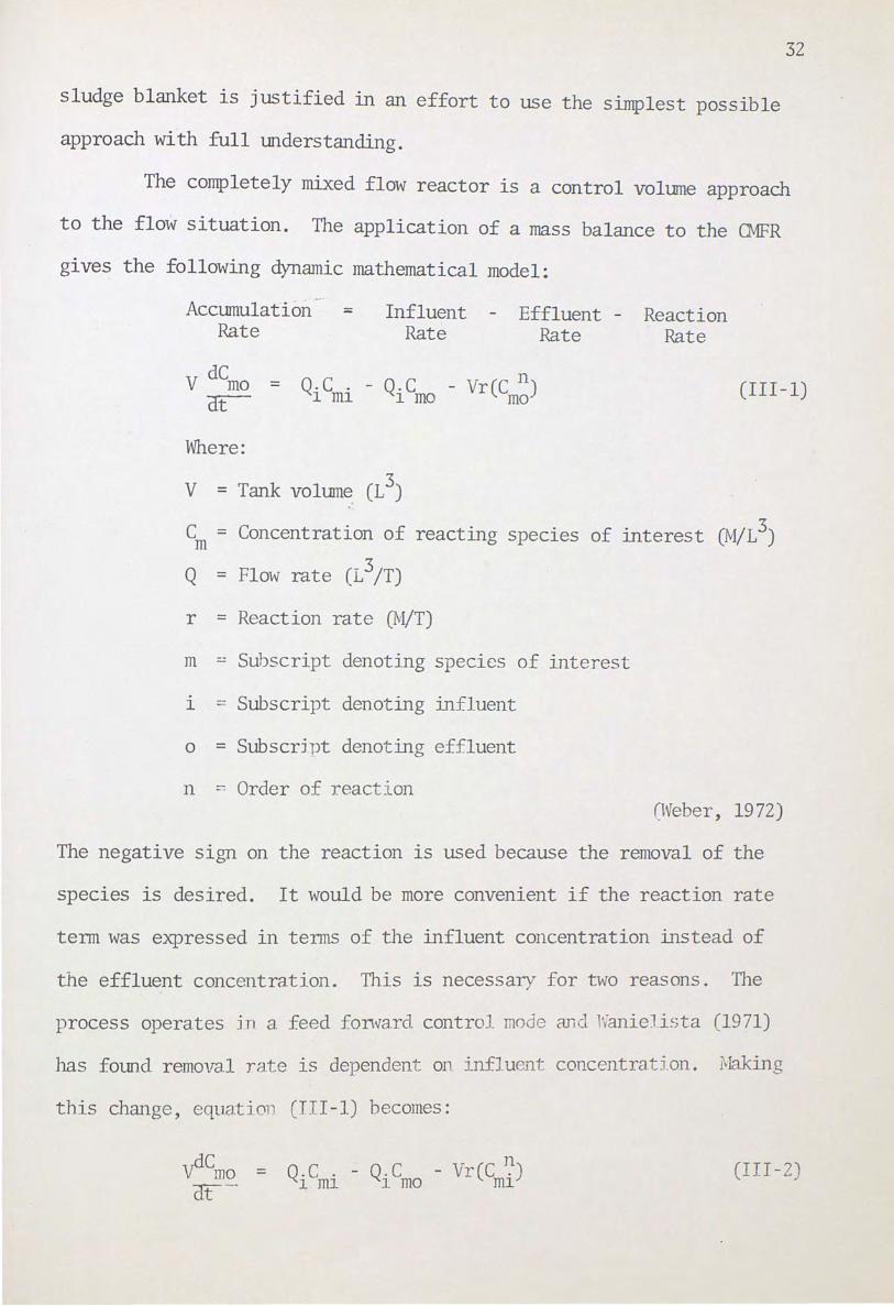
The completely mixed flow reactor is a control volume approach

to the flow situation. The application of a mass balance to the CMFR

gives the following dynamic mathematical model:

Accumulation = Rate

Influent Rate

Effluent Rate

V demo = Q.C . - Q.C - Vr(C n) err- 1 ffil 1 mo rna

Where:

V = Tank volume (13)

Reaction Rate

(III-1)

Cm = Concentration of reacting species of interest (M/13)

Q = Flow rate (L3/T)

r = Reaction rate (Jv1/T)

m = Subscript denoting species of interest

1 - Subscript denoting influent

o = Subscrjpt denoting effluent

n ~ Order of reaction (Weber, 19 72)

The negative sign on the reaction is used because the removal of the

species is desired. It would be more convenient if the reaction rate

tenn was expressed in tenns of the influent concentration instead of

the effluent concentration. This is necessary for two reasons. The

process operates jn a feed fon\fard control mod an :l Vaniel ista (1971)

has foliDd removal rate is dependent on influent concentration. Making

this change, equa.tio1. (III -1) becomes:

Q.C . - Q.C - Vr(C ~) 1 m1 1 rna m1

(III-2,

33

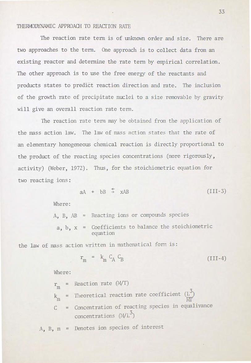
TiffiRMODYNAMIC APPROAQ-f TO REACTION RATE

The reaction rate tenn is of tm.known order and size. There are

two approaches to the tenn. One approach is to collect data from an

existing reactor and detennine the rate term by empirical correlation.

The other approach is to use the free energy of the reactants and

products states to preaict reaction direction and rate. The inclusion

of the growth rate of precipitate nuclei to a size removable by gravity

will give an overall reaction rate term.

The reaction rate term may be obtained from the application of

the mass action law. The law of mass action state~ that the rate of

an elementary homogeneous chemical reaction is directly proportional to

the product of the reacting species concentrations (more rigorously,

activity) (Weber, 1972). Thus, for the stoichiometric equation for

two reacting ions:

aA + bB t xAB (III-3)

Where:

A, B, AB = Reacting ions or compomds specles

a b X - Coefficients to balance the stoichiometric ; ' -

equation

the law of mass action written in mathematical fonn is·

Where:

= Reaction rate 0~/T) r m

k m

= TI1eoretical reaction rate coefficient (13)

lviT

(III-4)

c = Concentration of reacting species in equalivance

concentrations (M/13)

A, B, m = Denotes ion species of interest

34

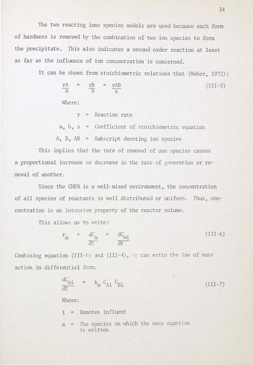
The two reacting 1ons species models are used because each form

of hardness is removed by the combination of two ion species to fonn

the precipitate. This also indicates a second order reaction at least

as far as the influence of ion concentration is concerned.

It can be shown from stoichiometric relations that (Weber, 1972):

rA = - a

Where:

rB o

= rAB --X

r = Reaction rate

a, b, x = Coefficient of stoichiometric equation

A, B, AB = Subscript denoting ion species

(III-5)

This implies that the rate of removal of one species causes

a proportional increase or decrease in the rate of generation or re-

moval of another.

Since the CNFR is a well-mixed environment, the concentration

of all species of reactants is well distributed or uniform. Thus, con-

centration is ah intensive property of the reactor vollUTle.

This allows us to 1vri te:

r m

= dC = m -a:r-

(III-6)

Combining equation (III-f) and (III-4), 1\~·-- can write tJ1c Jaw of mass

action in differential form.

=

Where:

k c". r_. m .M.l -Bl

1 = Denotes influent

m = The species on which the mass equat i on is written

(III -7)

35

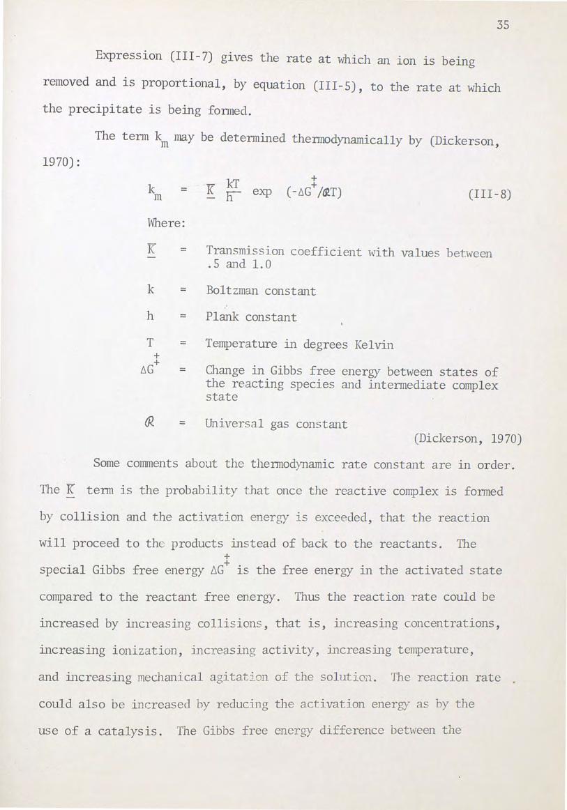
Expression (III-7) gives the rate at which an ion is being

removed and is proportional, by equation (III-5), to the rate at which

the precipitate is being fanned.

1970):

The term km may be determined thermodynamically by (Dickerson,

k m = · ·K ~ exp

+ +

( -11G /~T) (III-8)

Where:

K =

k =

h =

T =

=

=

Transmission coefficient with values between .5 and 1.0

Boltzman constant

Plank constant

Temperature in degrees Kelvin

Change in Gibbs free energy between states of the reacting species and intermediate complex state

Universal gas constant (Dickerson, 1970)

Some corrnnents about the thennodynarnic rate constant are in order.

The K tenn is the probability that once the reactive complex is fanned

by collision and the activation energy is exceeded, that the reaction

will proceed to the products instead of back to the reactants. The +

special Gibbs free energy ~G+ is the free energy in the activated state

compared to the reactant free energy. Thus the reaction rate could be

increased by increasing collisions, that is, increasing concentrations,

increasing ionization, increasing activity, increasing temperature,

and increasing mechanical agitation of the solutio11. The reaction rate

could also be increased by reducing the activation energy as oy the

use of a catalysis. The Gibbs free energy difference bet\\reen the

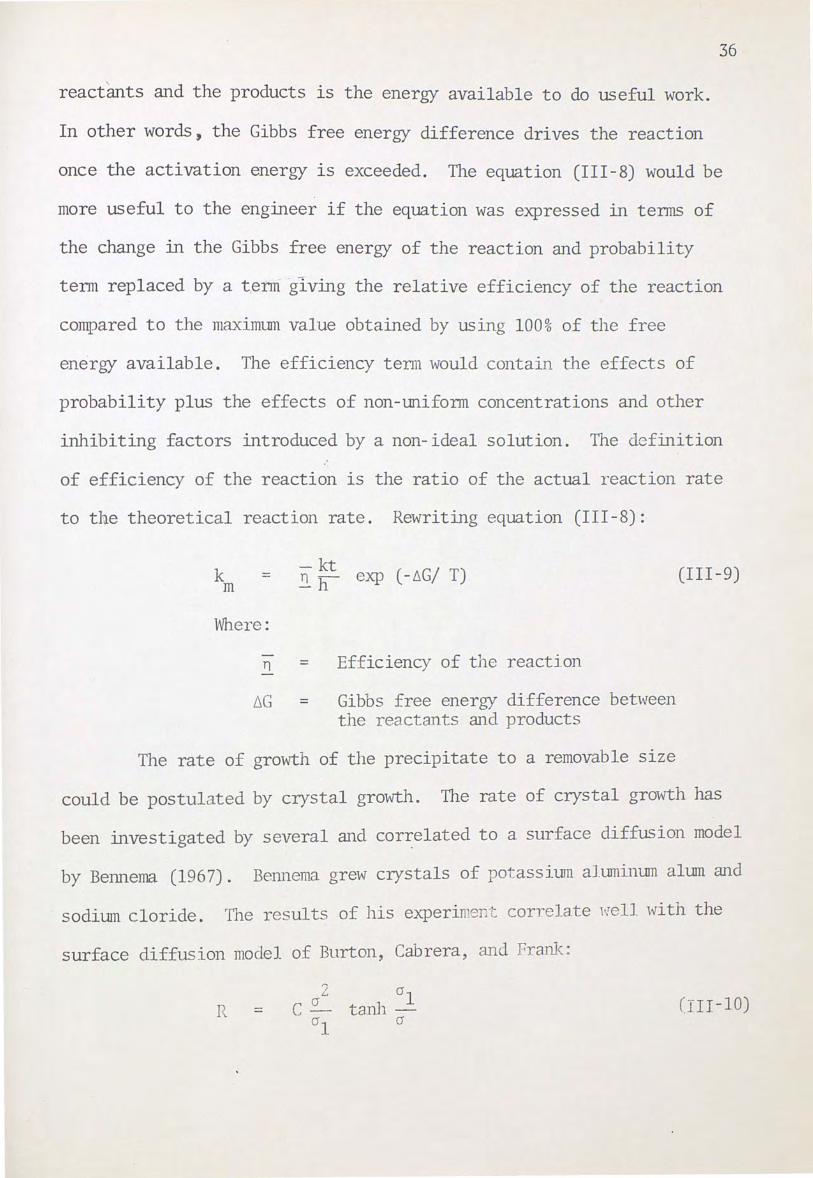
36

' reactants and the products is the energy available to do useful work.

In other words, the Gibbs free energy difference drives the reaction

once the activation energy is exceeded. The equation (III-8) would be

more useful to the engineer if the equation was expressed in terms of

the change in the Gibbs free energy of the reaction and probability

term replaced by a term giving the relative efficiency of the reaction

compared to the rnaximun value obtained by using 100% of the free

energy available. The efficiency term would contain the effects of

probability plus the effects of non-illlifonn concentrations and other

inhibiting factors introduced by a non-ideal solution. The definition

of efficiency of the reaction is the ratio of the actual reaction rate

to the theoretical reaction rate. Rewriting equation (III-8):

k = Til

Where:

n

~G

-kt 2l h exp (- 6G/ T)

=

=

Efficiency of the reaction

Gibbs free energy difference between the r eactants and products

The rate of growth of the precipitate to a removable s1ze

(III -9)

could be postulated by crystal growth. The rate of crystal growth has

been investigated by several and cor~elated to a surface diffusion model

by Bennema (1967). Bennema grew crystals of pot assium alumi num alum and

sodimn cloride. The results of his experin.ent correlate well with the

surface diffusion model of Burton, Cabrera, and Fr ank:

R = (I II-10)

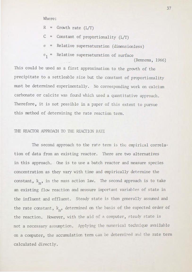
Where:

R = Growth rate (L/T)

c = Constant of proportionality (L/T)

cr = Relative supersaturation (dimensionless)

crl = Relative supersaturation of surface (Bennema, 1966)

This could be used as a first approximation to the growth of the

precipitate to a settleable size but the constant of proportionality

must be determined experimentally. No corresponding work on calcium

carbonate or calcite was found which used a quantitative approach.

Therefore, it is not possible in a paper of this extent to pursue

this method of determining the rate reaction term.

1HE REACTOR APPROAQ-I TO TI-IE REACTION RATE

37

The second approach to the rate te1111 is the empirical correla-

tion of data from an existing reactor. There are two alternatives

in this approach. One is to use a batch reactor and measure species

concentration as they vary with time and empirically determine the

constant, k , in the mass action law. The second approach is to take m

an existing flow reaction and measure important variables of state in

the influent and effluent. Steady state is then generally assumed and

the rate constant k , determined on the basis of the expected order of ' Jn

the reaction. However, with the aid of a computer, steady state is

not a necessary assumption. Applying ~he numerical teclmique available

on a computer, the accwnulation tenn can be determi='.ed and the rate tenn

calculated directly.

THE BATGI REACTOR

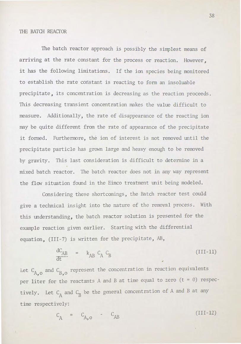
The batch reactor approach is possibly the simplest means of

arriving at the rate constant for the process or reaction. However~

it has the following limitations. If the ion species being monitored

to establish the rate constant 1s reacting to form an insoluable

38

precipitate~ its concentration 1s decreasing as the reaction proceeds.

This decreasing transient concentration makes the value difficult to

measure. Additionally, the rate of disappearance of the reacting ion

may be quite different from the rate of appearance of the precipitate

it formed. Furthermore, the ion of interest is not removed until the

precipitate particle has grown large and heavy enough to be removed

by gravity. This last consideration is difficult to determine in a

mixed batch reactor. The batch reactor does not in any way represent

the flow situation found in the Eimco treatment unit being modeled.

Considering these shortcomings, the Batch reactor test could

g1ve a technical insight into the nature of the removal process. With

this understanding~ the batch reactor solution is presented for the

example reaction given earlier. Starting with the differential

equation, (III-7) is written for the precipitate, AB,

dCAB err-

= (III-11)

Let CA and CB represent the concentration in reaction equivalents '0 ,o

per liter for the reactants A and B at time equal to zero (t = 0) respec-

tively. Let CA and CB be the general concentration of A and B at any

time respectively:

= c A,o CAB (III -12)

39

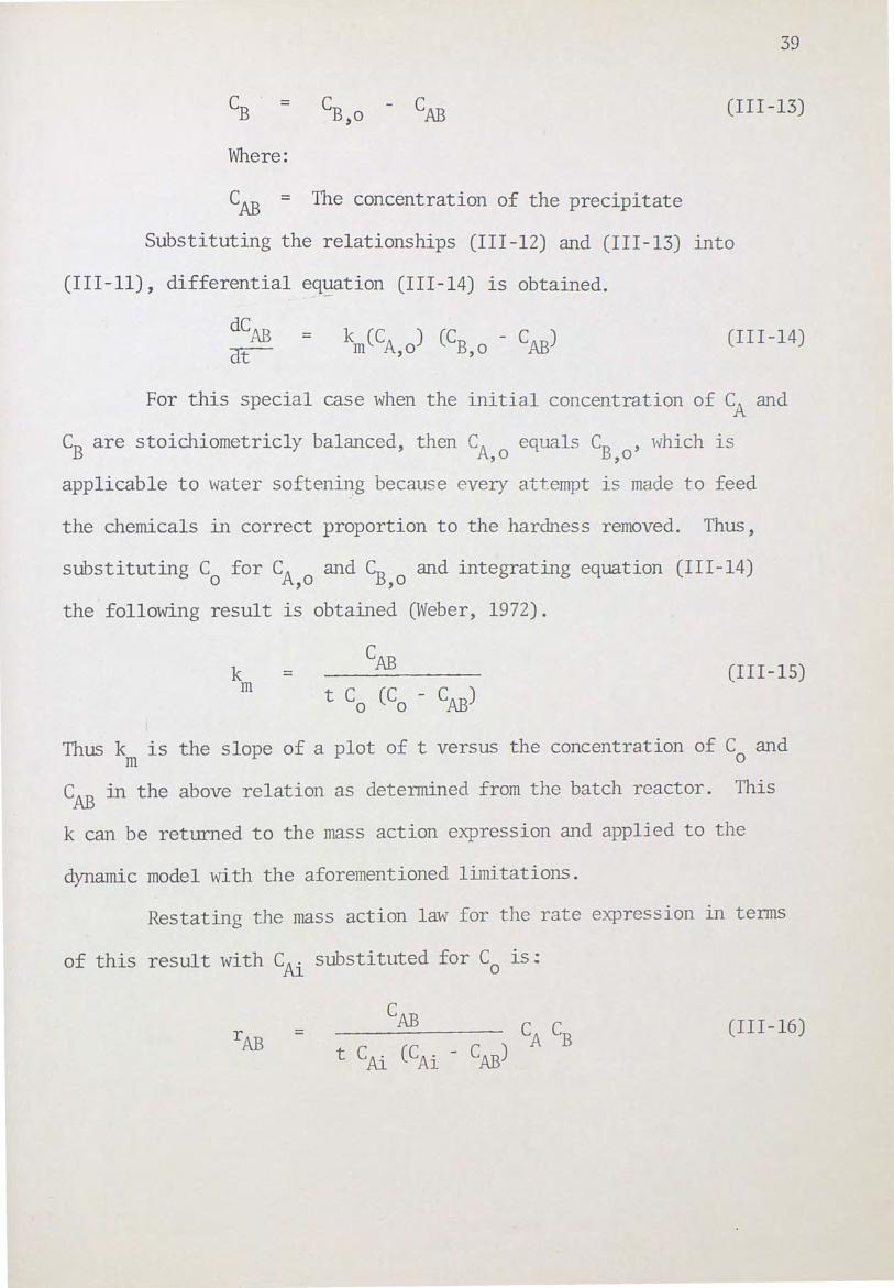
= CB - CAB ,o (III -13)

Where:

CAB = The concentration of the precipitate

Substituting the relationships (III-12) and (III-13) into

(III-11), differential equation (III-14) is obtained. -. - ·

= k (CA ) (CB - CAB) m J-\.,o ,o (III-14)

For this special case when the initial concentration of CA and

CB are stoichiometricly balanced, then CA equals CB , which 1s ,o ,o

applicable to water softening because every attempt is made to feed

the chemicals in correct proportion to the hardness removed. Thus,

substituting C for CA and CB and integrating equation (III-14) 0 .M.,O ,o

the following result 1s obtained (Weber, 1972).

k = m

(III-15)

Thus km 1s the slope of a plot of t versus the concentration of C0

and

CAB in the above relation as determined from the batch reactor. This

k can be returned to the mass action expression and applied to the

dynamic model with the aforementioned limitations.

Restating the mass action law for the rate expression in terms

of this result with CAi substituted for C0 is:

rAB = (III -16)

40

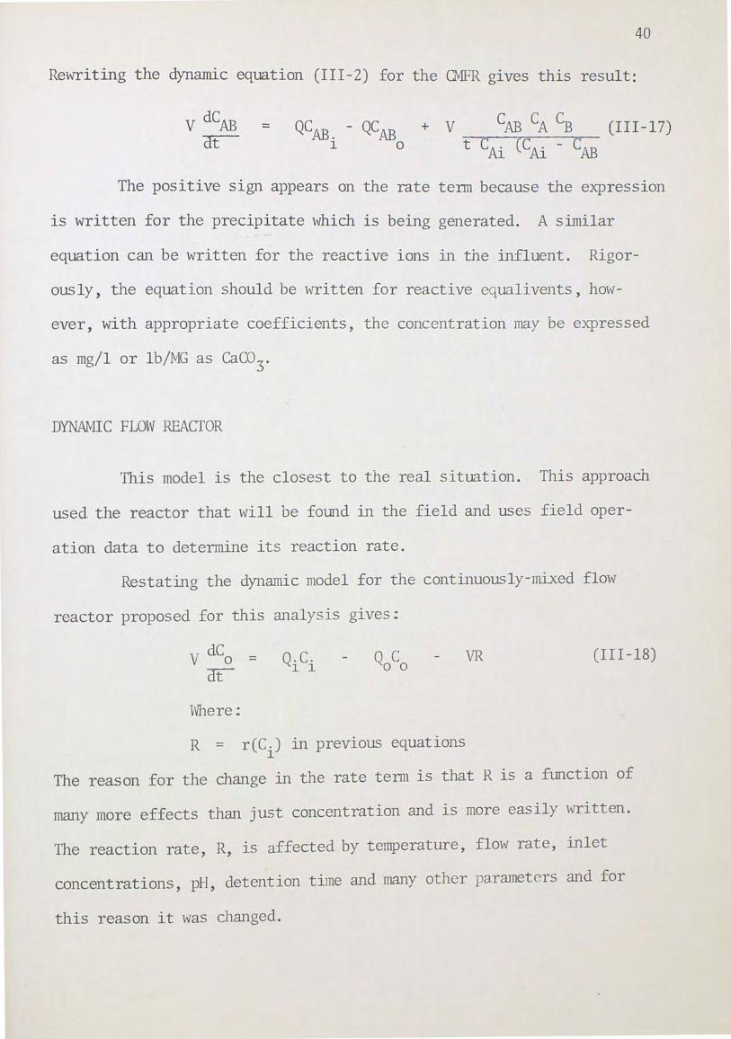
Rewriting the dynamic equation (III-2) for the CMFR gives this result:

V dCAB ~

= QCAB 0

+ V CAB CA CB (III-17) t CAi (CAi - CAB

The positive sign appears on the rate term because the expression

is written for the precipitate which is being generated. A similar

equation can be written for the reactive ions in the influent. Rigor­

ously, the equation should be written for reactive equalivents, how-

ever, with appropriate coefficients, the concentration may be expressed

as mg/1 or lb/MG as Caco3

.

DYNAivliC FLOW REACTOR

This model is the closest to the real situation . . This approach

used the reactor that will be found in the field and uses field oper-

ation data to determine its reaction rate.

Restating the dynamic model for the continuously-mixed flow

reactor proposed for this analysis gives:

V dCo =

~

Where;

Q.C. l l

R = r(C.) in previous equations l

VR (III-18)

The reason for the change in the rate term is that R is a function of

many more effects than just concentration and is more easily written.

The reaction rate, R, is affected by temperature, flow rate, inlet

concentrations, pH, detention time and many other parameters and for

this reason it was changed.

41

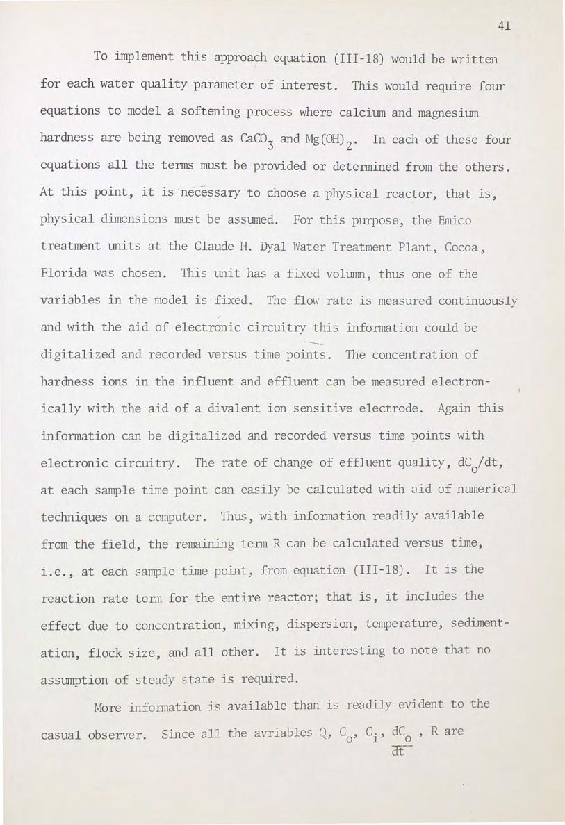
To implement this approach equation (III-18) would be written

f or each water quality parameter of interest. This would require four

equations to model a softening process where calcium and magnesium

hardness are being removed as Caco3 and Mg(OH)2

. In each of these four

equations all the terms must be provided or determined from the others.

At this point, it is -necessary to choose a physical reactor, that 1s,

physical dimensions must be assumed. For this purpose, the Emico

treatment units at the Claude H. Dyal 1Vater Treatment Plant, Cocoa~

Florida was chosen. This unit has a fixed volurnn, thus one of the

variables in the model is fixed. The flow rate is measured continuously

and with the aid of electronic circuitry this information could be --. digitalized and recorded versus time points. The concentration of

hardness ions in the influent and effluent can be measured electron-

ically with the aid of a divalent ion sensitive electrode. Again this

information can be digitalized and recorded versus time points with

electronic circuitry. The rate of change of effJuent quality, dC0/dt,

at each sample time point can easily be calculated with aid of numerical

techniques on a computer. Thus, with information readily available

from the field, the remaining tenn R can be calculated versus time,

i.e., at each c;ample time point, from equation (III-18). It is the

reaction rate tenn for the entire reactor; that is, it includes the

effect due to concentration, mixing, dispersion, temperature, sediment­

ation, flock size, and all other. It is interesting to note that no

assumption of steady state is required.

More in.fo1111ation is available than lS readily evident to the

casual observer. Since all the avriables Q, C0 , Ci' dC0 R are crt

42

recorded versus sample time points, they are unique to each other for

each sample time point. A sample time point is the location in time

when each variable is simultaneously measured and recorded. These sets

of data are represented in equation (III-19).

Measured Calculated

(tl, Q,- -c-, c.' . . . . dC , R) 0 1 0

(III-19) crt

Ctz' Q, c ' c.' . ) 0 1

(t3' Q, c ' c.' . . . . . ) 0 l

That is, R could be plotted versus corresponding data such as Q, C , 0

C., and dC at each sample· time point. 1 0

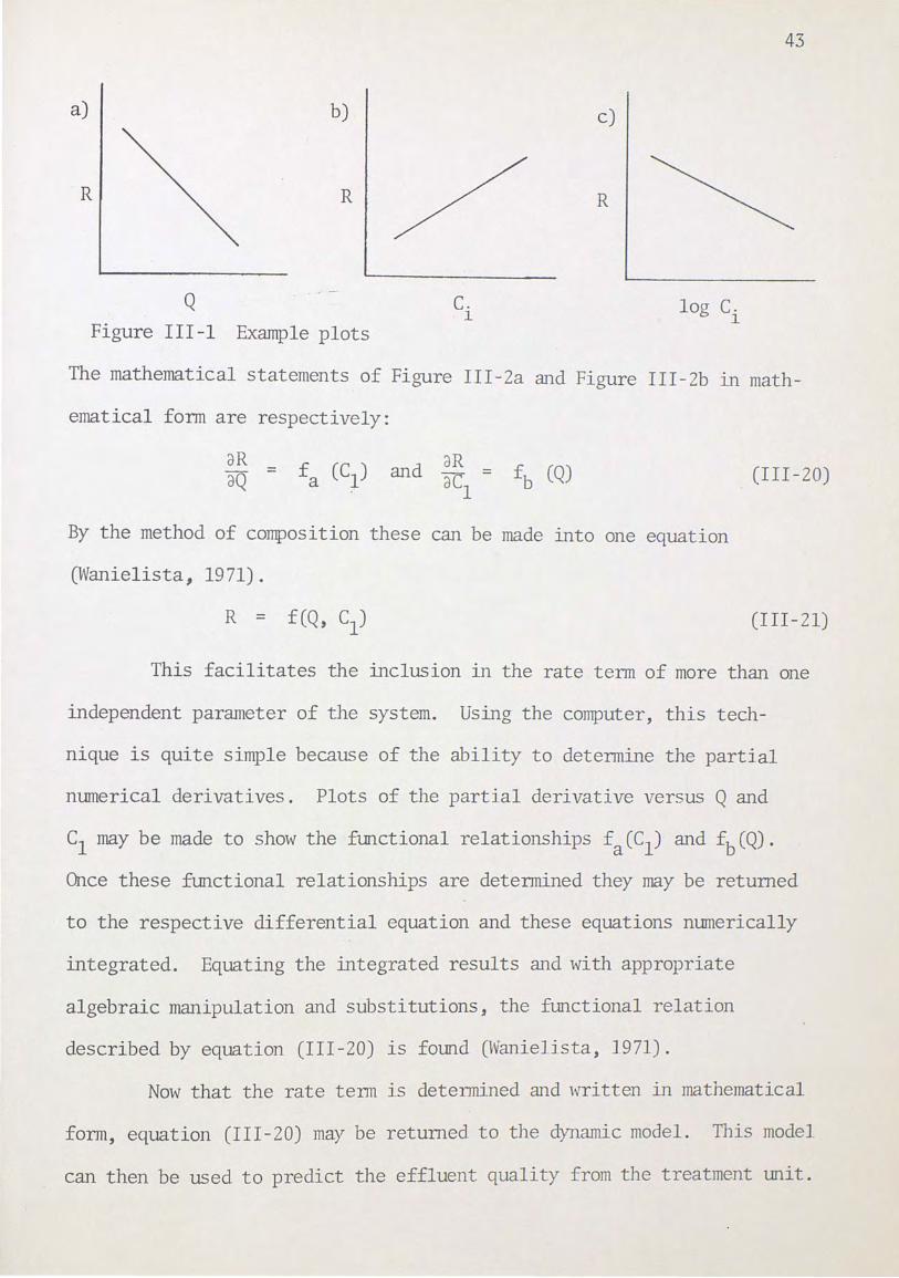
err-Hypothetical example plots of these time grouped parameters versus

the reaction rate are presented in Figure III-1. It is not intended to

infer these are straight lines, i.e., first order reaction, but that

this type of information is available. It is very probable that R is

a second order relation. Furthermorej pH, temperature, conductivity,

turbidity, and stirring RPIVI can be measured and digitalized in a

similar manner. These could also be plotted versus the reaction rate

and their effect accolUlted for. Additionally, the rate term could be

plotted versus parameters measured at some future or past time. For

example, plot R at time t versus Ci at time t - tD where tD is the

detention time of the treatment basin.

A further use of the parametric plots 1s to write differential

equations from the plots. By means of appropriate bookkeeping m1d

data search by the computer, it should be possible to obtain plots

using three variables. Examples of such plots are shown in Figure III-2.

a) b)

R R

Q Figure III-1 Example plots

c. l

c)

R

log C. l

43

The mathematical statements of Figure III-2a and Figure III-2b in math-

ematical form are respectively:

aR = aQ

By the method of composition these can be made into one equation

(Wanielista, 1971).

(III-20)

(III-21)

This facilitates the inclusion in the rate term of more than one

independent parameter of the system. Using the computer, this tech-

nique is quite simple because of the ability to determine the partial

numerical derivatives. Plots of the partial derivative versus Q and

c1 may be made to show the functional relationships fa(C1) and fb(Q).

Once these functional relationships are determined they may be returned

to the respective differential equation and these equations numerically

integrated. Equating the integrated results and with appropriate

algebraic manipulation and substitutions, the functional relation

described by equation (III-20) is found (Wanielista, 1971).

Now that the rate term is determined and written in mathematical

fonn, equation (III-20) may be returned to the dynamic model. This model

can then be used to predict the effluent quality from the treatment llllit.

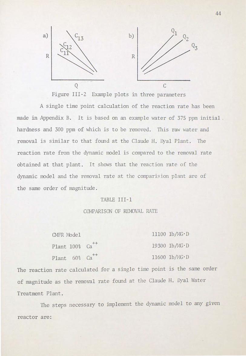
44

a) b)

R R

Q c Figure III-2 Example plots in three parameters

A single time point calculation of the reaction rate has been

made in Appendix B. It is based on an example water of 375 ppm initial

hardness and 300 ppm of which is to be removed. This raw water and

removal is similar to that found at the Claude H. Dyal Plant. The

reaction rate from the dynamic model is compared to the removal rate

obtained at that plant. It shows that the reaction rate of the

dynamic model and the removal rate at t he comparision plant are of

the same order of magnitude.

CMFR Model

Plant 100%

Plant 60%

TABLE III-1

COivfPARISON OF REMOVAL RATE

++ Ca

++ Ca

11100 lb/MG·D

19300 lb/1v1G·D

11600 lb/r~IG· D

The reaction rate calculated for a single time point 1s the same order

of magnitude as the removal rate found at the Claude H. Dyal Water

Treatment Plant.

The steps necessary to jmplement the dynamic model to any given

reactor are:

45

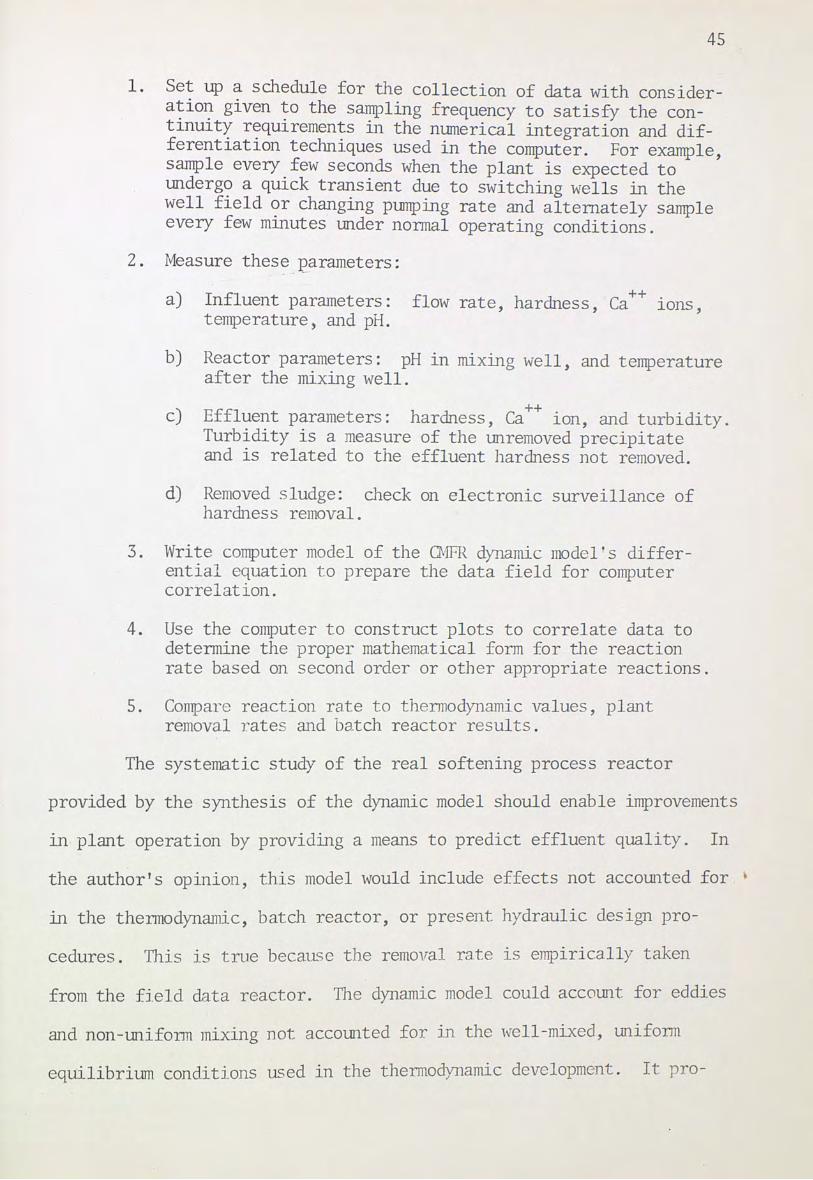
1. Set up a schedule for the collection of data with consider­a~ioJ?- given ~o the sal!lPling frequency to satisfy the con­tlnUlt~ r~qu1remen~s 1n the nliDlerical integration and dif­ferentlatlon techn1ques used in the computer. For example, sample every few seconds when the plant is expected to undergo a quick transient due to switching wells in the well field ?r changing pumping rate and alternately sample every few mlllutes under normal operating conditions.

2. Measure these E~rameters:

a) Influent parameters: temperature, and pH.

++ flow rate, hardness, Ca ions,

b) Reactor parameters: pH in mixing well, and temperature after the mixing well.

c) Effluent parameters: hardness, Ca++ ion, and turbidity. Turbidity is a measure of the unremoved precipitate and is related to the effluent hardness not removed.

d) Removed sludge: check on electronic surveillance of hardness removal.

3. Write computer model of the (}~R dynamic model!s differ­ential equation to prepare the data field for computer correlation.

4. Use the computer to construct plots to correlate data to determine the proper mathematical form for the reaction rate based on second order or other appropriate reactions.

5. Compare reaction rate to thennodynamic values, plant removal rates and batch reactor results.

The systematic study of the real softening process reactor

provided by the synthesis of the dynamic model should enable improvements

in plant operation by providing a means to predict effluent quality. In

the author's opinion, this model would include effects not accoLU1ted for ~

in the themodynamic, batch reactor, or present hydraulic design pro­

cedures. This is tn1e because the removal rate is empirically taken

from the field data reactor. The dynamic model could account for eddies

and non -unifonn mixing not accounted for in the well-mixed, mifonn

equilibrium concli tions used in the thennodynamic development. It pro-

vides a means of modeling the flow situations directly and does not

require the application of results from a non-flow situation as in a

batch reactor or jar test to a flow reactor.

46

SUMMARY AND CONCLUSIONS

IV. SUMMARY, CONCLUSIONS AND RECOMIV1ENDATIONS

Rcenemic studies have shown that water softening is worthwhile.

The aesthetic value of good tasting, potable water is appreciated by

everyone. The occasional reduction in dissolved solids along with the

reduced detergent usage with. soft water will help reduce the problems

of municipal wastewater treatment. Although softening may not be

required to meet public health service water quality criteria, the lime~

soda ash process does have good bacteria removal characteristics.

The ion exchange process when used for municipal softening 1s

not as economical as a line-soda ash process. It does not provide the

bacteria removal as does the lime-soda ash process. When softening

turbid and iron-rich water, the pretreatment required before 1on

exchange softening eliminates its simplicity and operational advantages.

However, lime-soda ash softening can be accomplished with the same

equipment as the turbidity and iron removal. Ion exchange does have

the advantages of automatic operation as well as pressure softening

units which eliminate double pumping for small, safe well supplies.

The lime-soda ash softening process removes hardness by pre­

cipitation of hardness caus1ng 1ons. The process follows the laws of

chemical reactions and thermodynamics lilltil the precipitate is formed.

At this point the minute particles coagulate, flocculate, and settle.

47

Removal is presently based on the settling velocity of the coagulated

and flocculated precipitate. Present designs are essentially based on

empirical detennination from years of trial and error. Systematic

parametric study seeill6 a rational alternative to advance the state of

the art.

48

The dynamic time response of a lime-soda ash process was

modeled. The continuously mixed flow reactor provided a reasonable

model for the combination rapid mixing basin, flocculator, and upflow

clarifier. Although the model does not provide for the hydraulics of

the settling process it does account for the slow approach to saturation

of magnesium hydroxide and calcium carbonate in supersaturated solu­

tions. The mathematical statement of the continuously mixed flow

reactor is simple enough to be easily handled by the computer and

articulated enough to show details of the parameters of influence.

The classical chemical thermodynamic approach to the problem

should predict the rate of formation of the precipitate. Review of the

literature on the subject gave several approaches to the problem from

collision theory to classical state theory using free energy. This

approach has been reviewed in this paper. However, the equation for

the determination of the rate of reaction requires the experimental

determination of one of the terms. It is therefore concluded by the

author that this approach could give no real solution to the numerical

problem except for an order of magnitude feeling. The rate of growth

of precipitate nuclei by the crystal growth mechanism was found to be

substantiated in the literature for a surface diffusion model. How­

ever, no work was found on the growth rate of calcium carbonate of mag­

nesium hydroxide, which simply implies the need for further research.

49

The second approach is the one widely used in chemical englneer­

mg: the use of a batch reactor to measure the reaction rate. This

process has some shortcomings. The batch reactor in either the stirred

or quiescent form is obviously not a flow situation. It is not possible

by this method to account for the flow disturbances and diffusion found

in a flow reactor. DifficUfties arise in the monitoring of the process

due to the desire to measure the removal rate by precipitation and

settling as opposed to just the reaction rate. Good estimates of

removal, chemical requirements and optimum precipitation conditions

can be obtained. However, it would be difficult to accurately predict

the removal rates of flow situations from the results of the batch

reactor tests.

The third approach 1s the author's attempt to eli1ninate some

of the ambiguities found in the two previous enlightened approaches.

The supposition that the dynamic time-varying model for the contin­

uously mixed stirred reactor does describe the combination up-flow

clarifier and rapid mixing basin is similar to the "black box" approach

to finding out what is in an electric circuit. The model is applied

to input and output data from the reactor and the effect of the reactor

1s determined. The approach allows the detailed study of each measur­

able parameter such as: pH, temperature, concentration, etc.

The investigation for the development of a model begins with

an existing reactor, in this case, the water softening units at the

Claude H. Dyal Treatment Plant. Field data is recorded on a time

point basis. That is, the parameters of the system are placed in a.

unique position based on their time of collection. The parametric

studies of the data are made with the aid of the computer. These

parametric plots represent functional relationships between indepen­

dent parameters and the dependent variable, removal rate of hardness.

Several of these parametric plots could be made into one mathematical

50

relationship using optimization, regression and composition techniques.

The final result would be a mathematical m~del of the up-flow clarifier

softening unit which could-be used to predict effluent quality for a

g1ven set of influent quality and quantity data.

The rate of removal of calcium hardness for an existing plant

was compared to the reaction rate for the dynamic model. The reaction

rate and removal rate were of the same order to magnitude. Therefore,

it may be concluded that the approach has considerable merit.

RECCMlY1ENDATIONS

It is recommended that data be recorded from the Claude H.

Dyal Treatment Plant to construct a mathematical model for the dynamic

time responses of the hardness removal process. The data should be

gathered in sufficient frequency to insure continuity for differ­

entiation and integration by the computer. This can be accomplished

by consulting continuity requirements of the numerical method used by

the computer. Parameters that should be measured in the raw water are:

++ flow rate, hardness, Ca 1on, temperature and pH. Parameters that

should be measured in the clarifier are: pH in the mixing well, tem­

perature after the mixing well. Clarifier effluent parameter which

should be measured are: hardness, Ca ++ ion, and turbidity.. The

monitoring of sludge removal and density could be a valuable check on

removal rate. The quantity and strength of the process chemical

51

must also be known.

A thoro~gh ooderstanding of the thennodynamics of chemical

reaction in solutions is necessary. Further, research into the growth

of crystal nuclei especially for calcium carbonate and magnesium

hydroxide is warranted. Possibly microscopic examination of precip­

itates and floccs found in -the sludge would be beneficial to an under­

standing of their growth. This information coupled with existing

literature on flocculation and coagulation should be compared to

results obtained by the dynamic modeling.

A review of reactor manufacutrer's literature is suggested to

see how they predict their removal rates and how these compared to

the results obtained from the dynamic modeling.

The overall objective of the paper was to propose a new

analytical tool for the evaluation and operation of water softening

plants. It is the belief of the author that the methodology may have

application to other flow processes and provide improved economics in

the operation of water softening plants .

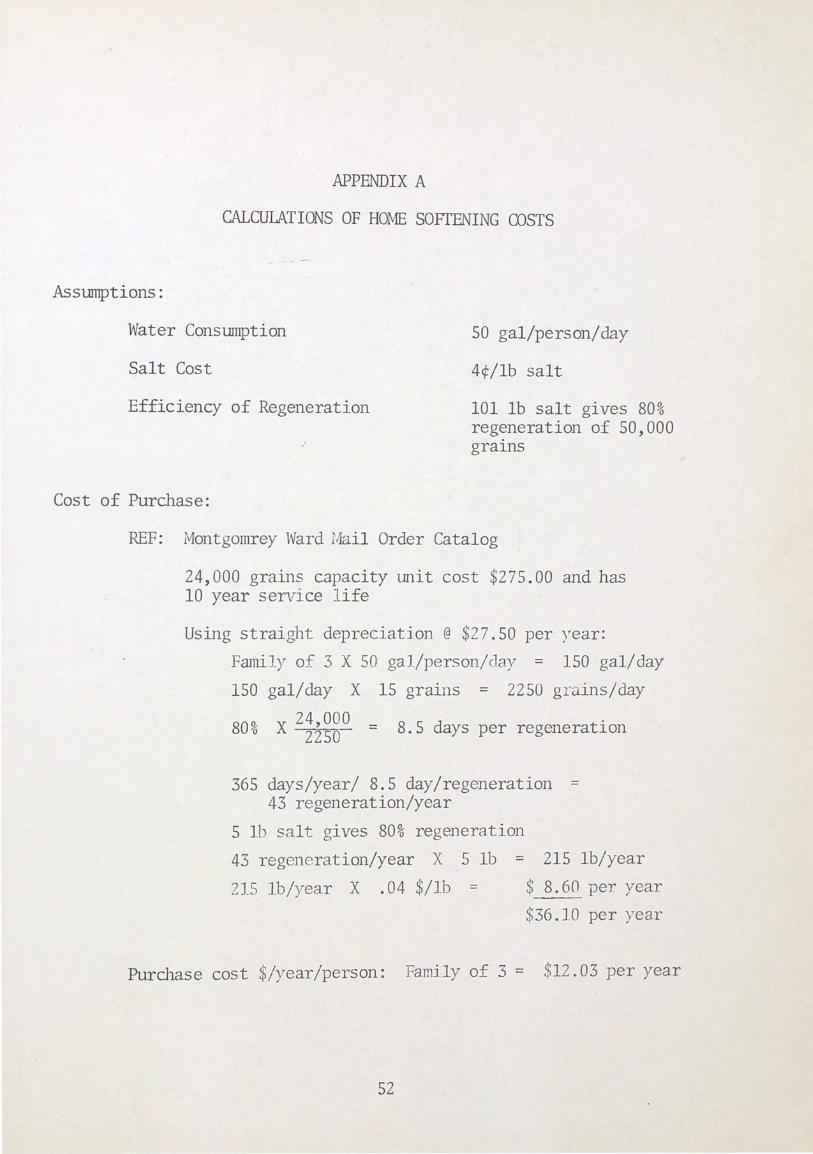
APPENDIX A

CALCUlATIONS OF HOME SOFTENING COSTS

Assumptions:

Water Consumption 50 gal/person/day

4¢/lb salt Salt Cost

Efficiency of Regeneration 101 lb salt gives 80% regeneration of 50,000 gralllS

Cost of Purchase:

REF: Montgomrey Ward l4ail Order Catalog

24,000 grains capacity unit cost $275.00 and has 10 year service l ife

Using straight depreciation@ $27. 50 per year:

Family of 3 X 50 gal/person/day = 150 gal/day

150 gal/day X 15 grains = 2250 grains/day

80% X 24 , 000 = 8.5 days per regeneration 2250

365 days/year/ 8.5 day/regeneration = 43 regeneration/year

5 ll salt gives 80% regeneration

43 regeneration/year X 5 lb =

215 lb/year X .04 $/lb =

215 lb/year

$ 8.60 per year

$36.10 per year

Purchase cost $/year/person: Family of 3 = $12.03 per year

52

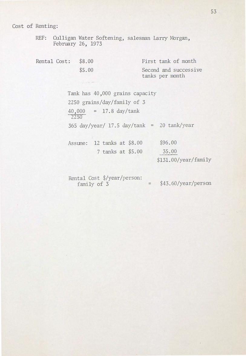
Cost of Renting:

REF: Culligan Water Softening, salesman Larry :tvlorgan, February 26, 1973

Rental Cost: $8.00

$5.00

First tank of month

Second and successive tanks per month

Tank has 40,000 gra1ns capacity

2250 grains/day/family of 3

40,000 = 17.8 day/tank 2250

365 day/year/ 17.5 day/tank = 20 tank/year

Assume: 12 tanks at $8.00 $96.00

7 tanks at $5.00 35.00

53

$131.00/year/family

Rental Cost $/year/person: family of 3 = $43.60/year/person

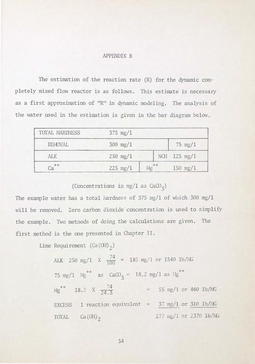
APPENDIX B

The· estimation of -the reaction rate (R) for the dynamic com-

pletely mixed flow reactor is as follows. This estimate is necessary

as a first approximation of "R" in dynamic modeling. The analysis of

the water used in the estimation is given in the bar diagram below.

TOTAL HARDNESS 375 mg/1

RBVDVAL 300 mg/1 75 mg/1

ALK 250 mg/1 I NCH 125 mg/1

Ca++ 225 rng/1 I Mg ++

150 mg/1

(Concentrations in mg/1 as CaC03)

The example water has a total hardness of 375 mg/1 of which 300 mg/1

will be removed. Zero carbon dioxide concentration is used to simplify

the example. Two methods of doing the calculations are given. The

first method is the one presented in Chapter II.

Lime Requirement (Ca(OH) 2)

ALK 250 mg/1 X 1b6 = · 185 mg/1 or 1540 lb/MG

++ ++ 75 mg/1 Mg as Caco3 = 18. 2 mg/1 as r·ig

M ++ ,8 ~ X . 74 g .J.. • [ , 24 0 3 = 55 mg/1 or 460 lb/MG

EXCESS 1 reaction equivalent = 37 mg/1 or 310 lb/MG

TOTAL Ca (OH) 2

2 77 mg/ 1 or 2370 lb/ l'·IG

54

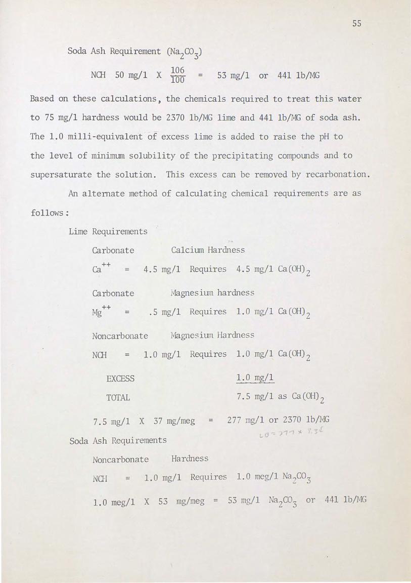
Soda Ash Requirement (Na2co3)

106 NQ-I 50 mg/ 1 X lOO =

55

53 mg/1 or 441 lb/MG

Based on these calculations, the chemicals required to treat this water

to 75 mg/ 1 hardness would be 2370 lb/MG lime and 441 lb/MG of soda ash.

The 1.0 milli-equivalent -of. excess lime is added to raise the pH to

the level of minimum solubility of the precipitating compounds and to

supersaturate the solution. This excess can be removed by recarbonation.

An alternate method of calculating chemical requirements are as

follows;

Lime Requirements

Carbonate Calcium Hardness

Ca++ = 4.5 mg/1 Requires 4.5 mg/1 Ca(OH) 2

Carbonate IVlagnes ium hardness

Mg ++

= .5 mg/1 Requires 1.0 mg/1 Ca(OH) 2

Noncarbonate Magnesium Hardness

NOH = 1.0 mg/1 Requires 1.0 mg/1 Ca(OH) 2

EXCESS 1.0 mg/1

TOTAL 7.5 mg/1 as Ca(OH) 2

7.5 mg/1 X 37 mg/meg = 277 mg/1 or 2370 lb/MG

Soda Ash Requirements t,IJ--== '1"1 .

Noncarbonate Hardness

NO-I = 1. 0 mg/1 Requirec; 1. 0 meg/1 1 a2co3

1.0 meg/1 X 53 mg/meg = 53 mg/1 Na2co... or 441 lb/MG .)

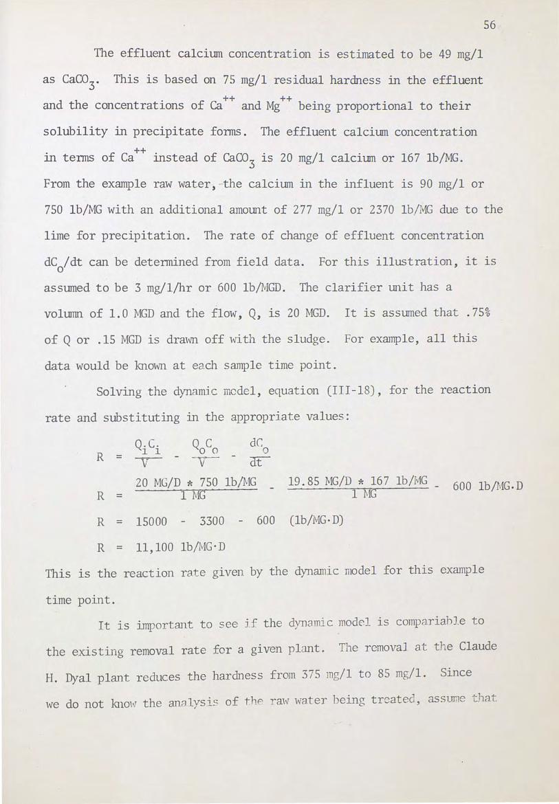
56

The effluent calcium concentration 1s estimated to be 49 mg/1

as Caco3. This is based on 75 mg/1 . residual hardness in the effluent . ++ ++

and the concentrat1ons of Ca and Mg being proportional to their

solubility in precipitate forms. The effluent calcium concentration

in terms of Ca++ instead of Caco3 is 20 ~g/1 calcium or 167 lb/MG.

From the example raw wat.er; -the calcium in the influent is 90 mg/1 or

750 lb/1'-.1G with an additional amount of 277 mg/1 or 2370 lb/MG due to the

lime for precipitation. The rate of change of effluent concentration

dC /dt can be determined from field data. For this illustration, it is 0

assrnned to be 3 mg/1/hr or 600 lb/MGD. The clarifier unit has a

volumn of 1.0 MGD and the flow, Q, is 20 MGD. It is assumed that .75%

of Q or .15 MGD is drawn off with the sludge. For example, all this

data would be known at each sample time point.

Solving the dynamic mcdel, equation (III-18), for the reaction

rate and substituting in the appropriate values:

Q.C. QOCO dr: R

l l 0 = v- v- at

20 MG/D * 750 lb/1viG 19.85 MG/D * 167 lb/MG 600 lb/MG.D R = 1 MG 1 MG

R = 15000 3300 600 (lb/MG· D)

R = 11,100 lb/MG· D

This is the reaction ro.te given by the dynamic model for this example

time point.

It is important to see if the dynamic model is compariahle to

the existing removal rate for a given plant~ The rcmovaJ at the Claude

H. Dyal plant reduces the hardness from 375 mg/1 to 85 mg/1. Since

we do not kno1 the anAlysis of the raw water being treated, assume t1at

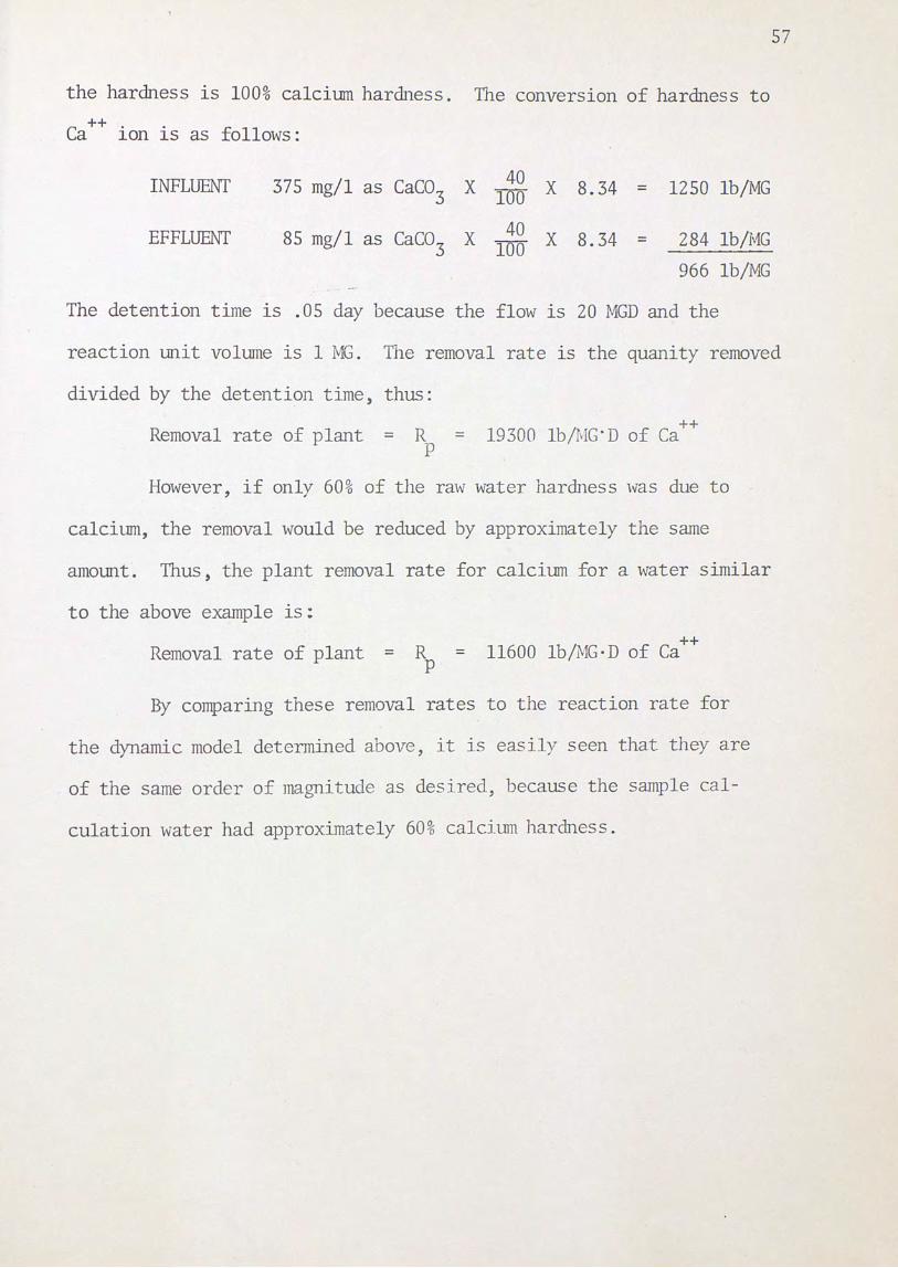
the hardness is 100% calcium hardness. The conversion of hardness to

Ca++ . . f 1on 1s as allows:

INFLUENT 40 375 mg/1 as Caco3 X TOO X 8.34 =

EFFLUENT 40 85 mg/1 as Caco3 X 100 X 8.34 =

1250 lb/MG

284 lb/MG

966 lb/MG

The detention time is .05 day because the flow is 20 MGD and the

57

reaction unit volwne is 1 MG. TI1e removal rate is the quanity removed

divided by the detenti~n time, thus:

Removal rate of plant = R = p

19300 lb/r··IG·D of Ca ++

However, if only 60% of the raw water haTdness was due to

calcit.nn, the removal would be reduced by approximately the same

amount. Thus, the plant removal rate for calcium for a water similar

to the above example is:

Removal rate of plant = R p = 11600 lb/MG·D of Ca

++

By comparing these removal rates to the reaction rate for

the dynamic model determined above, it is easily seen that they are

of the same order of magnitude as desired, because the sample cal­

culation water had approximately 60% calcium hardness.

LIST OF REFERENCES

American Water Works Association. Water Treatment Plant Design. New York: Arnerican.Water Works Association, 1969.

Aultman, W. N. "Synthetic Detergents as a Factor in Water Softening Economics". American Water Works Association Journal, L, October, 1958.

Bennema, P. "Experimental Confonnation of Solution Crystal - Growth Models". Crystal Growth, Proceedings of an Internat ional Conference on Crystal Growth, Boston, 20-24 June, 1966, a S:upplement to Physics and Chemistry _of Sol1dS. Edited by H. Steffen Peiser. Dxforn: Pergamon Press, 1967.

Dickerson, Richard E., Gray, Harry B., and Haight, Gilbert P. Jr. Chemical Principles . New York: W. A. Benjamin, 19 70.

Fair, Gordon M., Geyer, John C., and Okum, Daniel A. r'Water and Wastewater Engineering". Vol II: Water Purification and Wastewater Treatment and Disposal. New York: John Wiley and Sons, 1968.

National Advisory Corrunittee to the Secretary of the Interior. "Report of the Corrunittee". Water Quality Criteria. Washington D.C.: Federal Water Pollution Control Administration, 1968.

Riehl, ~~Ierrill L. Water Supply and Treatment. Washington D.C.: National Lime Associat1on, 1962.

Sawyer, Clair N., and McCarty, Perry L. Olemistry for Sanitary Engineers. New York: McGraw Hill, 1967.

U.S. Department of Health, Education, and Welfare. Public Health Service Drinking Water Standards, 1962 . Public Health Service PUblication No. 956. Washington D.C.: U.S. Government Printing Office _, 1962.

Wanielista, M. P. "An Evaluation of the Design and Operation of Water Treatment Facilities". Unpublished Ph.D. disertation, Cornell University, 1971.

Wanielista _, M. P., and Fa.lkson, L. M. "Flexibility in Water Treatment Plant Design". Journal American Water 1.Yorks Association, LXIII~ May, 1971.

58

59

Weber, Walter J. Ph siocochemical Processes for Water ality Control New York: 1 ey Intersc1ence, 1 72.

World Almanac and Book of Facts. New York: Newspaper Enterprise ASsoc1ation, 1971.