lable at ScienceDirect

Marine Environmental Research xxx (2014) 1e18

Contents lists avai

Marine Environmental Research

journal homepage: www.elsevier .com/locate/marenvrev

An index based on the biodiversity of cetacean species to assess theenvironmental status of marine ecosystems

Arianna Azzellino a, b, *, Maria Cristina Fossi c, Stefania Gaspari d, Caterina Lanfredi a, b,Giancarlo Lauriano e, Letizia Marsili c, Simone Panigada b, Michela Podest�a f

a Politecnico di Milano, DICA, Piazza Leonardo da Vinci, 32, 20133 Milano, Italyb Tethys Research Institute, viale Gadio, 2, 20121 Milano, Italyc Dpt. of Physical, Earth and Environ. Sciences, University of Siena, Via PA Mattioli 4, 53100 Siena, Italyd Universit�a degli Studi di Firenze, Dipartimento di Biologia, Via Madonna del Piano 6, 0019 Sesto Fiorentino, FI, Italye Institute for Environmental Protection and Research (ISPRA), Via Brancati, 60, 00144 Roma, Italyf Museum of Natural History of Milan, C.so Venezia 55, 20121 Milano, Italy

Keywords:MSFDGood Environmental StatusBiodiversityAnthropogenic pressuresGenetic markers

* Corresponding author. Politecnico di Milano, DIC32, 20133 Milano, Italy.

E-mail address: arianna.azzellino@polimi.it (A. Az

http://dx.doi.org/10.1016/j.marenvres.2014.06.0030141-1136/© 2014 Elsevier Ltd. All rights reserved.

Please cite this article in press as: Azzellino, Amarine ecosystems, Marine Environmental

a b s t r a c t

The Marine Strategy Framework Directive (MSFD) requires the assessment of the environmental status inrelation to human pressures. In this study the biodiversity of the cetacean community is proposed asMSFD descriptor of the environmental status and its link with anthropogenic pressures is investigated.Functional groups are generally favoured over indicator species since they are thought to better reflect toanthropogenic stressors. Cetaceans are in many situations the most well known component of pelagicecosystems. Their habitat requirements are known and can be used to evaluate the theoretical biodi-versity that should be expected in a certain area. The deviations between the theoretical biodiversity andthe actual biodiversity may be used to detect the impacts of human activities. Based on this analysisfishery resulted to be by far the most significant of the existing pressures. Among all the species, bot-tlenose dolphin was found the most correlated with the fishery sector dynamics.

© 2014 Elsevier Ltd. All rights reserved.

1. Introduction

The EU environmental policies during the last three decadeshave focused on determining adverse and undesirable changes tothe natural system as the result of human activities and then, ifsuch changes are detected, management responses are thenforeseen to alleviate those adverse changes. The Marine StrategyFramework Directive (hereinafter MSFD) and before the WaterFramework Directive (WFD) might be both considered as com-ponents of a suite of environmental controls linked on their ownto the Directives for Environmental Impact Assessment, StrategicEnvironmental Assessment, Nitrates control and the Habitats andSpecies and Wild Birds Directives (Borja et al., 2010). The MSFDestablishes a framework for the development of marine strategiesdesigned to achieve the “Good Environmental Status” (GES) in themarine environment, by the year 2020, using 11 qualitative

A, Piazza Leonardo da Vinci,

zellino).

., et al., An index based on theResearch (2014), http://dx.do

descriptors. The descriptors are not objectives per se: rather, theydescribe features of the ecosystem that are widely considered asimportant, either from a conservation (e.g., biodiversity, foodweb) or threat (e.g., non-indigenous species, marine litter)perspective that may be useful in developing a specific set ofmanagement objectives. Therefore, the MSFD requires theassessment of the functioning of each objective in relation topressures. Based on this knowledge, appropriate programs ofmeasures might be enforced to control the pressures that signif-icantly affect the marine environmental status. Understanding themechanism and/or the hierarchical pathways through whichspecific activities affect descriptor indicators is an essential step inthe process of managing their potential impact. This assessment isfurther complicated by the fact that specific impacts may resultfrom activities associated with numerous sectors (Ban et al.,2010). Thus, the link between sectors, the pressures theygenerate and the effects that those pressures have on the com-ponents of the ecosystem, need to be clearly understood if theimpact of a sector and its activities is to be reduced or mitigated toavoid detrimental effects to the ecological characteristics of theecosystem.

biodiversity of cetacean species to assess the environmental status ofi.org/10.1016/j.marenvres.2014.06.003

Table 1Criteria and associated indicators for the MSFD Descriptor 4 (food webs).

Attribute Criterion Indicator

Energy flow in the foodweb

Productivity of keyspecies or trophicgroup (4.1)

Performance of keypredator species usingtheir production perunit biomass (4.1.1)

Structure of the foodweb (size)

Proportion of selectedspecies at the top of thefood web (4.2)

Large fish (by weight)(4.2.1.)

Structure of the foodweb (abundance)

Abundance/distribution of keytrophic groups/species(4.3)

Abundance trends offunctionally importantselected groups/species(4.3.1)

Table 2List of criteria for selecting key species/groups for indicator 4.3.1 “Abundance/dis-tribution of key trophic species” as proposed by the Commission Decision (2010/477/EU).

Criterion Indicator Selection criteria for keytrophic groups/species

Abundance/distribution ofkey trophic groups/species (4.3)

Abundance trendsof functionallyimportant selectedgroups/species(4.3.1)

(i) Groups with fastturnover rates(ii) Groups/species that aretargeted by humanactivities or that areindirectly affected by them(iii) Habitat-defininggroups/species(iv) Groups/species at thetop of the food web(v) Long-distanceanadromous andcatadromous migratingspecies(vi) Groups/species that aretightly linked to specificgroups/species at anothertrophic level

A. Azzellino et al. / Marine Environmental Research xxx (2014) 1e182

There are numerous human activities that have the potential tonegatively impact marine ecosystems (Halpern et al., 2007), manyof which are common to several sectors functioning in Europe'sregional seas. MSFD identifies 18 specific pressures, which could beplaced into one of eight general pressure groupings based on theirshared impact characteristics such as whether the pressure causedphysical damage (e.g., abrasion or selective extraction), physicalloss (e.g., smothering or sealing) or contamination (e.g., introduc-tion of synthetic compounds) (see Annex III of the Directive [EC2008] for the full list of pressures and impacts).

Among the other MSFD descriptors, descriptor 4 (D4) addressesthe marine food webs and states “All elements of the marine foodwebs, to the extent that they are known, occur at normal abundanceand diversity and levels capable of ensuring the long-term abundanceof the species and the retention of their full reproductive capacity”.

It is well known that human activities may cause direct or in-direct changes in food webs (Layman et al., 2005; Raffaelli, 2005).Events such as overexploitation (Pauly et al., 1998), pollution (Boonet al., 2002), eutrophication (Cloern, 2001), habitat fragmentationand destruction (Layman et al., 2007; Melian and Bascompte,2002), invasions of species (Vander Zanden et al., 1999) andanthropogenic climate change (Kirby and Beaugrand, 2009; Murenet al., 2005) all pose potential threats to the structure and dynamicsof food webs, acting at variable spatial scales and affecting foodwebs in different ways (Moloney et al., 2010).

To successfully identify and then monitor all these processes isextremely challenging. To date, ecologists have proposed severalquantitative indicators to describe the status of marine ecosystems.However, strengths and weaknesses of the different indicators areusually only partially known. In many cases, due to the gaps in ourknowledge about the relationship of the ecological status with theexisting pressures, these indicators fail to support the setting ofmanagement objectives and do not allow the provision of scientificadvice on how these objectives might be achieved. This is partic-ularly true for indicators based on multiple species. In spite of that,marine foodweb indicators are becoming increasingly important asa factor in conservation management, particularly concerning theassessment of the ecological risk deriving fromhuman activities (deRuiter et al., 2005; Sala and Sugihara, 2005). In contrast to thesingle-species approaches, a system-level approach is in factconsidered attractive since both, direct and indirect effects ofdisturbance are integrated into a single interaction network(Raffaelli, 2005). However, due to the high functional diversity inmarine ecosystems and to the food-web complexity, practical ap-plications remain quite rare. Whilst an ecosystem perspective isincreasingly used in fisheries management to study ecosystem re-sponses to different stressors and to assure sustainable use of re-sources (e.g. Coll et al., 2008), similar holistic approaches toevaluate the combined influences of other anthropogenic stressorson food webs are still lacking.

In this study, the biodiversity of the cetacean community isproposed as MSFD D4 indicator (e.g. indicator 4.3.1 Abundancetrends of functionally important selected groups/species) andreference points are provided to correlate the environmental statusderived by this indicator with the pressures affecting the study area(i.e. naval traffic, pollution, fishing pressure etc.).

Fig. 1. Study area: The three subregions under the Italian jurisdiction are shown.

1.1. The MSFD D4 descriptor and cetacean species

The D4 indicators stipulated in the Commission Decision (Eu-ropean Commission, 2010; 2010/477/EU), following extensive re-view by the JRC/ICES Task Group (TG4) on food webs (Rogers et al.,2010), address three criteria related to food web structure andenergy transfer between different components (Table 1).

Please cite this article in press as: Azzellino, A., et al., An index based on themarine ecosystems, Marine Environmental Research (2014), http://dx.do

As shown in Table 1, whereas criterion 4.1 and its associatedindicator 4.1.1 is proposed mainly as a proxy measure of energyflow within marine food webs, structural properties of foodwebs are covered by criteria 4.2 and 4.3 (Table 1). Given that

biodiversity of cetacean species to assess the environmental status ofi.org/10.1016/j.marenvres.2014.06.003

Fig. 2. Aerial surveys. Upper section: survey transects; lower section: sightings. Bp: fin whales, Pm: sperm whales, Gg: Risso's dolphins, Gm: long-finned pilot whales, Sc: stripeddolphins, Tt: common bottlenose dolphins and Zc: Cuvier's beaked whales.

A. Azzellino et al. / Marine Environmental Research xxx (2014) 1e18 3

many food webs components are also relevant to other MSFDdescriptors (e.g. D1, biodiversity, D3, commercial fish speciesand D6; seafloor integrity), it might be expected that indicatorsused for D4 overlap those used for the other Descriptors. The

Please cite this article in press as: Azzellino, A., et al., An index based on themarine ecosystems, Marine Environmental Research (2014), http://dx.do

criteria for selecting key species/groups to calculate indicator4.3.1, are stated in the previously mentioned Commission Deci-sion and relate to many possible food web components(Table 2).

biodiversity of cetacean species to assess the environmental status ofi.org/10.1016/j.marenvres.2014.06.003

A. Azzellino et al. / Marine Environmental Research xxx (2014) 1e184

Marine mammals, and particularly cetacean species, respond tomost of these criteria. B�anaru et al. (2013) in their study about thetrophic structure in the Gulf of Lions marine ecosystem have foundthat dolphins are keystone species. Power et al. (1996) definedkeystone as species with a structuring role within ecosystems andthe food webs that interconnect in spite of a relatively low biomassand hence food intake. Keystone species strongly influence and arestrongly influenced by the abundances of other species and theecosystem dynamic (Piraino et al., 2002) and may reasonably beconsidered key species for the indicator 4.3.1.

2. Material and methods

2.1. Study area

This study concerns the three Mediterranean subregions, whichhave been considered for the Initial Assessment of the Italian ma-rine waters, namely the Western Mediterranean Sea, the AdriaticSea and the Ionian and Central Mediterranean Sea (Fig. 1).

Fin whales (Balaenoptera physalus), sperm whales (Physetermacrocephalus) Risso's dolphins (Grampus griseus), longfinned pilotwhales (Globicephala melas), striped dolphins (Stenella coeru-leoalba), common bottlenose dolphins (Tursiops truncatus) andCuvier's beaked whales (Ziphius cavirostris) are known as regularlyoccurring species (Boisseau et al., 2010) in the Mediterranean Sea.Short-beaked common dolphins (Delphinus delphis), although alsooccurring, are much rarer (Bearzi et al., 2003).

For the purpose of the analysis the study area was covered bygrid of 2490 cell units with a size of 17 � 22 km. Such a grid hasbeen used for all the presented spatial analysis.

2.2. Used data set

For the purpose of this study two different types of data wereused: sighting data deriving from the aerial surveys funded by theItalian Ministry of the Environment, and conducted respectively inthe Pelagos Sanctuary (see Panigada et al., 2011a), in the Tyr-rhenian, and Ionian Seas (see Panigada et al., 2011b; Lauriano et al.,2011); and the strandings data available from the Italian StrandingNetwork.

2.2.1. Sightings from the aerial surveysSurveys were designed following the ‘distance sampling’

method to estimate abundance (Buckland et al., 2001; see Fig. 2). Inall the surveys, the study area was subdivided into strata, followingbathymetric criteria and the available knowledge of cetaceanpresence and distribution. Due to the seasonality of fin whalepresences, surveys in subarea 1 and 2 were conducted both in thehigh presence season (i.e. summer) and in the low presence season(i.e. winter). Parallel line transects, 10 or 15 km apart, with arandom starting point were determined using the program Dis-tance ver. 5.0 (http://www.ruwpa.st-and.ac.uk/distance/), to allowfor- homogeneous coverage probability. Survey methods aredescribed in detail in Panigada et al., 2011a. Table 3 shows the mainfeatures of the aerial survey data set.

2.2.2. Strandings dataData on cetacean strandings along the Italian coasts have been

regularly collected on a national basis between 1986 and 2005 bythe Centro Studi Cetacei. The network managed the monitoring ofItalian coasts and the study of the strandings, bycatches and shipcollisions. Since 2006 the Italian database of strandings (BDS) is thenational archive of these data and provides information about thedate of the event, its location, data of the specimen such as species,gender and, length. The considered records, updated to 2012, hold

Please cite this article in press as: Azzellino, A., et al., An index based on themarine ecosystems, Marine Environmental Research (2014), http://dx.do

information about toxicological and parasitological investigations,description of samples collected and the institute where the sam-ples are stored. The considered data set contains little more than4000 records, belonging to 14 species. These historical strandings ofMediterranean species along Italian coastline are available on linehttp://mammiferimarini.unipv.it (Podest�a et al., 2006, 2009).

2.2.3. Observed biodiversity: DAR index based on sightings/strandings data

The ratio between DominanceSp (i.e. number of sightings of thedominant species over total number of sightings. The dominantspecies is the one with the highest frequency in the cell unit) andthe Relative AbundanceAll Spp (i.e. total number of sightings nor-malised over the maximum abundance value recorded in the studyarea) considering all the species was chosen as biodiversity index.

DAR ¼ DominanceSpRel:AbundanceAll spp

Such an index was preferred to other known diversity indexessince it relies on dominance and relative abundance which are bothconcepts well known to researchers studying cetacean species.Moreover dominance and relative abundance can be easily deter-mined based on cetacean census data.

DAR index is inversely correlated to diversity. It increases in lowbiodiversity conditions, where largely dominant species are pre-sent and determine almost entirely the abundance, and decreaseswhen the biodiversity increases and the presence of dominantspecies is balanced by the presence of other species.

Fig. 3 shows how the DAR index increases as dominance in-creases and decreases as the relative abundance increases. Asensitivity analysis of DAR index was performed and its variabilitywas compared with the one of the most well known Shannon'sdiversity index (see Supplementary material S1 and S2).

2.2.4. Expected biodiversity based on habitat availabilityPresence/absence habitat models using physiographic pre-

dictors as covariates were used to estimate the presence probabilityof the six species of cetaceans regularly occurring in the study area(due to the fact we had very few sightings and stranding records oflong finned pilot whale the species was not considered in thisstudy) and to obtain the theoretical biodiversity (i.e. expected)based on such habitat availability. Most of the used models weredeveloped based on long-term data series (see Azzellino et al., 2012for reference). The habitat availability for the species Cuvier'sbeaked whale was instead obtained from a much shorter data se-ries. However, model accuracy in this case was validated evaluatingthe model performance in an area different from the calibration(see Azzellino et al., 2011 for details). The physiographic predictorsfor the study area have been obtained through the GEBCO Oneminute Digital Atlas and gridded by means of a GIS software. Seabed slope was calculated according to Burrough (1986).

Based on the habitat model predictions, a map was obtained forthe expected biodiversity. Predictions were produced for every cellunit (Fig. 4) and the 75% probability was assumed as thresholdvalue for the species presence.

2.2.5. Anthropogenic pressuresShip traffic, pollution, and impact of fisheries were considered to

explain the patterns of the biodiversity deviations from the ex-pected. Particularly, the maritime traffic density was derived fromthe results of PASTA-MARE project, pollution data were obtainedfrom the EIONET Archive (European Environment Information andObservation Network) which concerns sediments and biota. andthe fishery impact of was evaluated through the statistics available

biodiversity of cetacean species to assess the environmental status ofi.org/10.1016/j.marenvres.2014.06.003

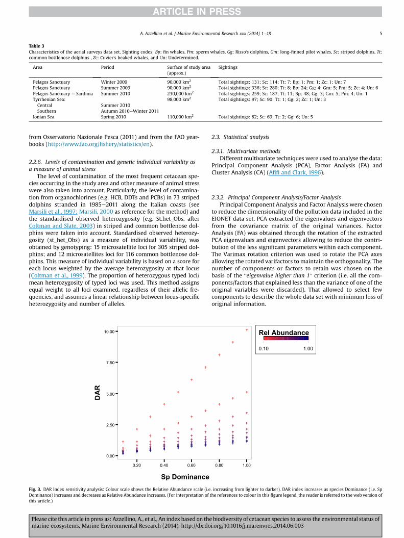
Table 3Characteristics of the aerial surveys data set. Sighting codes: Bp: fin whales, Pm: sperm whales, Gg: Risso's dolphins, Gm: long-finned pilot whales, Sc: striped dolphins, Tt:common bottlenose dolphins , Zc: Cuvier's beaked whales, and Un: Undetermined.

Area Period Surface of study area(approx.)

Sightings

Pelagos Sanctuary Winter 2009 90,000 km2 Total sightings: 131; Sc: 114; Tt: 7; Bp: 1; Pm: 1; Zc: 1; Un: 7Pelagos Sanctuary Summer 2009 90,000 km2 Total sightings: 336; Sc: 280; Tt: 8; Bp: 24; Gg: 4; Gm: 5; Pm: 5; Zc: 4; Un: 6Pelagos Sanctuary e Sardinia Summer 2010 230,000 km2 Total sightings: 259; Sc: 187; Tt: 11; Bp: 48; Gg: 3; Gm: 5; Pm: 4; Un: 1Tyrrhenian Sea: 98,000 km2 Total sightings: 97; Sc: 90; Tt: 1; Gg: 2; Zc: 1; Un: 3Central Summer 2010Southern Autumn 2010eWinter 2011

Ionian Sea Spring 2010 110,000 km2 Total sightings: 82; Sc: 69; Tt: 2; Gg: 6; Un: 5

A. Azzellino et al. / Marine Environmental Research xxx (2014) 1e18 5

from Osservatorio Nazionale Pesca (2011) and from the FAO year-books (http://www.fao.org/fishery/statistics/en).

2.2.6. Levels of contamination and genetic individual variability asa measure of animal stress

The level of contamination of the most frequent cetacean spe-cies occurring in the study area and other measure of animal stresswere also taken into account. Particularly, the level of contamina-tion from organochlorines (e.g. HCB, DDTs and PCBs) in 73 stripeddolphins stranded in 1985e2011 along the Italian coasts (seeMarsili et al., 1997; Marsili, 2000 as reference for the method) andthe standardised observed heterozygosity (e.g. St.het_Obs, afterColtman and Slate, 2003) in striped and common bottlenose dol-phins were taken into account. Standardised observed heterozy-gosity (st_het_Obs) as a measure of individual variability, wasobtained by genotyping: 15 microsatellite loci for 305 striped dol-phins; and 12 microsatellites loci for 116 common bottlenose dol-phins. This measure of individual variability is based on a score foreach locus weighted by the average heterozygosity at that locus(Coltman et al., 1999). The proportion of heterozygous typed loci/mean heterozygosity of typed loci was used. This method assignsequal weight to all loci examined, regardless of their allelic fre-quencies, and assumes a linear relationship between locus-specificheterozygosity and number of alleles.

Fig. 3. DAR Index sensitivity analysis: Colour scale shows the Relative Abundance scale (i.eDominance) increases and decreases as Relative Abundance increases. (For interpretation of tthis article.)

Please cite this article in press as: Azzellino, A., et al., An index based on themarine ecosystems, Marine Environmental Research (2014), http://dx.do

2.3. Statistical analysis

2.3.1. Multivariate methodsDifferent multivariate techniques were used to analyse the data:

Principal Component Analysis (PCA), Factor Analysis (FA) andCluster Analysis (CA) (Afifi and Clark, 1996).

2.3.2. Principal Component Analysis/Factor AnalysisPrincipal Component Analysis and Factor Analysis were chosen

to reduce the dimensionality of the pollution data included in theEIONET data set. PCA extracted the eigenvalues and eigenvectorsfrom the covariance matrix of the original variances. FactorAnalysis (FA) was obtained through the rotation of the extractedPCA eigenvalues and eigenvectors allowing to reduce the contri-bution of the less significant parameters within each component.The Varimax rotation criterion was used to rotate the PCA axesallowing the rotated varifactors to maintain the orthogonality. Thenumber of components or factors to retain was chosen on thebasis of the “eigenvalue higher than 1” criterion (i.e. all the com-ponents/factors that explained less than the variance of one of theoriginal variables were discarded). That allowed to select fewcomponents to describe the whole data set with minimum loss oforiginal information.

. increasing from lighter to darker). DAR index increases as species Dominance (i.e. Sphe references to colour in this figure legend, the reader is referred to the web version of

biodiversity of cetacean species to assess the environmental status ofi.org/10.1016/j.marenvres.2014.06.003

Fig. 4. Map of the expected biodiversity (i.e. number of expected species). Species presence predictions are produced based on physiographic predictors through the species habitatmodels.

A. Azzellino et al. / Marine Environmental Research xxx (2014) 1e186

2.3.3. K-means Cluster AnalysisA K-means Cluster Analysis (CA) was used to analyse the habitat

similarities among the cell units. The cell areas of potential habitatfor the six species were the input of the analysis. The EuclideanDistance was chosen as distance measure:

d2�xi; xj

� ¼ffiffiffiffiffiffiffiffiffiffiffiffiffiffiffiffiffiffiffiffiffiffiffiffiffiffiffiffiffiffiffiffiffiffiXq

k¼1

�xik � xjk

�22

vuut

CA was run twice. The final cluster centroids obtained from thefirst run were used as initial centres of the second run.

Fig. 5. Characteristics of the habitat types identified through the K-mean ClusterAnalysis. habitat type 1: coastal habitat, habitat type 2: pelagic habitat, habitat type 3:shelf break and continental slope habitat. Abbreviations: Bp habitat: typical habitat ofthe species fin whale, Pm habitat: typical habitat of the species sperm whale, Gghabitat: typical habitat of the species Risso's dolphin, Gm habitat: typical habitat of thespecies long-finned pilot whale, Sc habitat: typical habitat of the species striped dol-phin, Tt habitat: typical habitat of the species common bottlenose dolphin and Zchabitat: typical habitat of the species Cuvier's beaked whale.

2.3.4. Hypothesis testingStatistical significance of the differences was assessed by non-

parametric hypothesis testing. Particularly KruskaleWallis testwas used to compare K independent samples and the Man-neWhitney test was used for the comparison of 2 independentsamples. The correlation between biodiversity deviations from theexpected and the anthropogenic pressures were quantified throughthe Pearson's correlation coefficient or the Spearman's rank corre-lation coefficient depending on variable skewness.

3. Results

3.1. Classification of the habitat types

The K-means Cluster Analysis applied to the areas of potentialhabitat (i.e. areas with species presence probability higher than75%) of the six species in the 2490 cell units. CA allowed the

Please cite this article in press as: Azzellino, A., et al., An index based on the biodiversity of cetacean species to assess the environmental status ofmarine ecosystems, Marine Environmental Research (2014), http://dx.doi.org/10.1016/j.marenvres.2014.06.003

Fig. 6. Map of the three habitat types identified through K-means CA.

A. Azzellino et al. / Marine Environmental Research xxx (2014) 1e18 7

identification of 3 categories of habitats (Fig. 5): habitat type 1:coastal habitat (bottlenose dolphin habitat is dominant), habitattype 2: pelagic habitat (almost homogeneous presence of stripeddolphin, fin whale, sperm whale and Cuvier's beaked whale habi-tats), habitat type 3: shelf break and continental slope habitat(sperm whale, Risso's dolphin and Cuvier's beaked whale habitatsprevail). Themap of the habitat types is shown in Fig. 6. The averagephysical characterics of the habitat types are shown in Table 4.

3.2. Biodiversity assessment through the DAR index

The biodiversity was assessed through the DAR index, andcalculated based on the sightings available from the aerial surveys.For the purpose of the comparative analysis, the study area wassubdivided into the subareas shown in Fig. 7 and, to avoid the over-

Table 4Physical characteristics of the habitat types.

Habitat types Mean Std. deviation Median Minimum Maximum

Type 1 Depth (m) 300 657 50 20 2800Slope (m/m) 1.4 0.8 1.9 0.0 2.0

Type 2 Depth (m) 2961 475 2790 2021 4000Slope (m/m) 1.8 0.4 2.0 0.0 2.0

Type 3 Depth (m) 1554 485 1521 422 3044Slope (m/m) 2.0 0.1 2.0 0.9 2.0

Please cite this article in press as: Azzellino, A., et al., An index based on themarine ecosystems, Marine Environmental Research (2014), http://dx.do

representation of the area with the highest effort, only the 2010campaign (see Table 3) was used to evaluate the DAR index in thesubareas 1 and 2. Data from aerial surveys were not available forsubareas 0 and 6 but they were considered in the analysis of thestrandings.

DAR indexes of the different subareas were tested through aKruskal Wallis test which revealed that the 5 subareas hadsignificantly different biodiversity values (chi-square: 23.1, df: 4,P < 0.001). A multiple comparison ManneWhitney test wherethe Bonferroni correction (i.e. P/k comparisons) was applied,revealed that subareas 1, 2 and 3 are homogenous in terms ofbiodiversity (P > 0.0125) as subareas 4 and 5 (P > 0.0125). On theother hand, subareas 4 and 5 have a significantly lower biodi-versity than subareas 1, 2, 3 (ManneWhitney test P < 0.001, seeFig. 8).

3.3. Expected biodiversity based on habitat availability

Grounding on the fact that subareas 1, 2 and 3 were found tohave the highest biodiversity values, only these subareas wereconsidered to attribute a DAR index value to the habitat typesdescribed in the paragraph 3.1. All the sightings available from theaerial surveys conducted in the area (see Table 3) were used tocalculate the DAR index to be associated to the habitat types.Table 5 shows the results of these evaluations.

biodiversity of cetacean species to assess the environmental status ofi.org/10.1016/j.marenvres.2014.06.003

Fig. 7. Map of the 7 subareas. Subarea 0: Adriatic Sea Subarea 1: Western Ligurian Sea; Subarea 2: Eastern Ligurian and upper Tyrrhenian Sea; Subarea 3: West Sardinia; Subarea 4:Central and Southern Tyrrhenian Sea; Subarea 5: Ionian Sea and Gulf of Taranto; Subarea 6: Strait of Sicily.

A. Azzellino et al. / Marine Environmental Research xxx (2014) 1e188

Based on these estimates it was possible to obtain the expectedbiodiversity as function of the availability of potential habitats forall the subareas. The expected DAR index for each subarea wasevaluated as the weighted mean of the DAR indexes of the habitattypes as function of their percent coverage of the total area (seeTable 6).

As shown in Table 6 some relevant deviations between theactual and the expected biodiversity were observed for subareas 2(Eastern Ligurian and upper Tyrrhenian) 4 (Central and lowerTyrrhenian) and 5 (Ionian). Particularly observed DAR indexes inthese subareas are higher than the expected values, possiblyrevealing a loss of biodiversity.

Fig. 8. DAR index distribution of the 5 subareas. For the sake of comparison only the2010 survey data were used for subareas 1 (Western Ligurian Sea) and 2 (EasternLigurian Sea and upper Tyrrhenian Sea). The boxes show the median, the quartiles, theminimum and maximum values.

Please cite this article in press as: Azzellino, A., et al., An index based on themarine ecosystems, Marine Environmental Research (2014), http://dx.do

3.4. DAR index evaluated on strandings

With the exception of very few studies (Haelters et al., 2006;Hart et al., 2006; Pierce et al., 2007; Camphuysen, 2010; Peltieret al., 2012) to date only few attempts have been made to inferinformation on marine species distribution from stranding data.Strandings, in fact, are generally thought to be disjointed, bothspatially and temporally, from the open sea habitats and the cor-responding uses of the species. However, it has been proved thatthe proportions of species in the stranding records well reflect therelative abundance of live animals of the species living in therespective region (Pyenson, 2010, 2011). Also in our study area suchcorrespondence between the proportion of the species frequenciesin the strandings and in sighting records is confirmed (see Fig. S1).

Following this line of thought, the DAR index was applied to thestranding records available for the Italian coasts (see Fig. 9). Theused data series spans from 1986 up to 2012 and consists of 4222records.

The same grid used for the sightings has been used to analysethe strandings data. The differences among subareas have beentested using Kruskal Wallis test that resulted to be significant (chi-square: 24.7, df: 6, P < 0.001) only when the Adriatic subarea wasincluded (see Fig. 10).

Excluding the Adriatic Sea, which was shown to have a lowerbiodiversity (i.e. higher DAR index), all the other subareas wereshown to have the same level of biodiversity (chi-square: 8.61, df: 5,P: 0.126).

Table 5DAR index of the three habitat types. The index is estimated based on the sightingsavailable from all the aerial conducted in subareas 1, 2 and 3.

Habitat type N Mean Median Minimum Maximum Percentiles

Valid 25 50 75

Type 1 62 4.73 3.67 0.00 11.00 0.00 3.67 11.00Type 2 160 5.99 5.50 0.00 11.00 2.26 5.50 11.00Type 3 115 7.35 11.00 0.00 11.00 3.67 11.00 11.00

biodiversity of cetacean species to assess the environmental status ofi.org/10.1016/j.marenvres.2014.06.003

Table 6Observed and expected DAR index of the subareas. The observed DAR index is the median value of cell units in the subarea calculated based on the sightings (see paragraph3.2). The Expected DAR index is the weighted mean of the DAR indexes of the habitat types as function of their percent coverage of the total area. In bold the observed DARvalues higher than the expected.

Zone % Over total area Expected DAR index Observed DAR index

Habitat type 1 Habitat type 2 Habitat type 3

(0) Adriatic 98.7 0.4 0.9 3.51 e

(1) W Ligurian 44.3 42.9 12.7 3.64 3.67(2) E Ligurian and upper Tyrrhenian 88.3 1 10.7 3.62 5.50(3) Sardinia 63.2 26 10.9 3.63 1.72(4) Central and lower Tyrrhenian 35.3 29.3 35.3 3.91 11.00(5) Ionian 24.4 56.6 19 3.72 5.50(6) Strait of Sicily 90.7 5.2 4.2 3.55 e

A. Azzellino et al. / Marine Environmental Research xxx (2014) 1e18 9

As Fig. 11 shows, both the correlation matrix and the corre-sponding scatter plots, reveal a high coherence between the Ex-pected DAR index, evaluated based on the habitat availability andthe Observed DAR index, calculated on sightings (r: 0.908). On theother hand, a sort of inverse correlation can be seen between DARindexes evaluated either on sightings or on strandings.

That seems to be the direct consequence of the Tyrrhenian andSardinia subareas where the DAR indexes evaluated on strandingssuggest an inverse pattern than the indexes evaluated on sight-ings (e.g. DAR indexes calculated on strandings respectively sug-gest a lower biodiversity for Sardinia and a higher biodiversity forTyrrhenian Sea). Off course it must be remarked that while thestranding records span over several years, the evaluation based onsightings is almost instantaneous. Reasonably the DAR index

Fig. 9. Map of the available stranding re

Please cite this article in press as: Azzellino, A., et al., An index based on themarine ecosystems, Marine Environmental Research (2014), http://dx.do

evaluated on strandings reflects the biodiversity occurring overthe whole period. That is the case of the Western Sardinia andCentral and lower Tyrrhenian areas where the DAR index vari-ability in time reveals a slightly higher biodiversity in the Tyr-rhenian area (see Fig. S2), although the difference is notstatistically significant. Table 7 shows the Spearman's rank cor-relations of DAR index and the index components (i.e. Scdom:dominance of the species striped dolphin; Ttdom: dominance ofthe species bottlenose dolphin and RelAbund: Relative Abundanceconsidering all the species) evaluated on strandings versus thetime series. It can be observed that both Ttdom and RelAbund showa positive trend with the year while the time trend is inverseconcerning DAR index (see Table 7). These trends are also shownin Fig. 12.

cords (time series for 1986e2012).

biodiversity of cetacean species to assess the environmental status ofi.org/10.1016/j.marenvres.2014.06.003

Fig. 10. DAR index calculated on stranding records of the 7 subareas. The box shows the median, the quartiles, the minimum and maximum values.

A. Azzellino et al. / Marine Environmental Research xxx (2014) 1e1810

3.5. Biodiversity and human pressures

In order to correlate the biodiversity pattern of the differentareas with the existing pressures, some pre-processing of the datawas required. Particularly, Principal Component Analysis and FactorAnalysis (hereinafter PCA and FA) was needed to reduce thedimensionality of the pollution data included in the EIONET dataset, and some spatial processing was needed either to interpolateship traffic densities and to associate the fishing pressure indicatorsto every subarea.

3.5.1. PCA/FA of the EIONET data setPCAwas applied to both the EIONET sediment and the biota data

set. As far as sediments were concerned PCA extracted 7

Fig. 11. Correlation analysis of DAR indexes: Expected (i.e. evaluated based on habitat availaevaluated on strandings). Scatter plots are also shown. It can be observed that the subarea

Please cite this article in press as: Azzellino, A., et al., An index based on themarine ecosystems, Marine Environmental Research (2014), http://dx.do

components, globally explaining 88.9% of the total variance. Norotation criterion was applied since the extracted principal com-ponents were clean enough to be interpreted. As shown in Table 8,most of the variance is explained by PAHs and PCBs, respectivelyconstituting the first and the second component, globallyexplaining little less than 60% of the explained variance. Metalswere separated on different components.

Factor Analysis was instead applied to the biota data set. TheVarimax rotation of the principal components allowed in this caseto have the pollutants well distributed over the components and itfacilitated the interpretation (see Table 9). As for sediments, 7components were extracted, globally explaining 79.5% of the totalvariance. Factor loadings revealed that PAHs and PCBs are morelinked in the biota, most of the compounds lying on the first rotated

bility), Observed (sightings) (i.e. evaluated on sightings) and Observed (strandings) (i.e.s Sardinia and Tyrrhenian have a string leverage for all the correlations.

biodiversity of cetacean species to assess the environmental status ofi.org/10.1016/j.marenvres.2014.06.003

Table 7Correlation analysis between DAR index and DAR index components (i.e. Scdom: dominance of striped dolphin; Ttdom: dominance of bottlenose dolphin and RelAbund:Relative Abundance considering all the species) evaluated on the strandings and the corresponding time series. The correlations are shown in terms of Spearman's rankcorrelation coefficient.

Year Scdom Ttdom RelAbund DARindex

Spearman's rho Year Correlation coefficientSig. (2-tailed)N

Scdom Correlation coefficient �0.034Sig. (2-tailed) 0.171N 1593

Ttdom Correlation coefficient 0.148a �0.408a

Sig. (2-tailed) 0.000 0.000N 1593 1593

RelAbund Correlation coefficient 0.399a 0.134a 0.199a

Sig. (2-tailed) 0.000 0.000 0.000N 1593 1593 1593

DARindex Correlation coefficient �0.067a 0.511a 0.270a �0.260a

Sig. (2-tailed) 0.008 0.000 0.000 0.000N 1593 1593 1593 1593

a Correlation is significant at the 0.01 level (2-tailed).

A. Azzellino et al. / Marine Environmental Research xxx (2014) 1e18 11

component. Pesticides such as DDT and its residues and beta-HBHstrongly correlate with the third rotated component whichexplained alone little more than 10% of the variance. Metals fell ondifferent components also in this case, but their reciprocal corre-lations were found different from the correlations found in sedi-ments (e.g. in biota data set Cr, Cu and Zn are weakly correlated andlie on the same component of the Tributyltin compounds, whereasCd and Hg that were separated on different components in thesediment analysis, correlate both with the seventh biota compo-nent explaining 4% of the total variance).

The extracted components from both the sediment and thebiota data set, were used to summarise the pollution informationfor the different subareas.

3.5.2. Spatial interpolation of the ship traffic densitiesAs explained in the Methods, maritime traffic density data

were derived from the results of PASTA-MARE project. These datawere interpolated by using an Inverse Distance Weighted algo-rithm (IDW, Webster and Oliver, 2001), which assumes that eachinput point has a local influence that diminishes with distance.So the points closer to the processing cell have greater weightthan more distant points. The graduated colour scale shown inFig. 13 is the result of the IDW interpolator applied to the analysisgrid.

Fig. 12. DAR index and components trends over the studied period. Scdom: dominanceAbundance considering all the species.

Please cite this article in press as: Azzellino, A., et al., An index based on themarine ecosystems, Marine Environmental Research (2014), http://dx.do

Based on these values, an average naval density was attributedto every subarea.

3.5.3. Fishery impactsFAO statistics could only be associated to the whole study area,

so no pre-processing of these data was attempted to disaggregatethese statistics to the subarea level. On the other hand, the statisticsavailable from Osservatorio Nazionale Pesca (2011) were moredetailed and available at the scale of the Italian regions (seeTable 10), so they could be processed and associated to the sub-areas. Particularly, the statistics available from the OsservatorioNazionale Pesca were attributed to each subarea as function of thecoastline length of each Italian region falling within the subareaborders.

3.5.4. Biodiversity deviations from the expected and correlationwith pressures

As it was described in the paragraph 3.3, some relevant de-viations of the actual biodiversity from the one expected werefound in some subareas. The deviations of the DAR index, observedand expected (see Table 6), were correlated with all the indicatorsof human pressures described so far. The resulting correlationmatrix is shown in Table 11.

of striped dolphin; Ttdom: dominance of bottlenose dolphin and RelAbund: Relative

biodiversity of cetacean species to assess the environmental status ofi.org/10.1016/j.marenvres.2014.06.003

Table 8Principal Component Analysis of the Sediments EIONET data set: the factor loadings of the 7 components extracted are shown. Factor loadings higher than 0.5 and lowerthan �0.5 are shown in bold. The percent and cumulative variance explained by each components are also shown.

Components

1 2 3 4 5 6 7

Aldrin �0.111 �0.017 �0.111 �0.113 �0.384 0.483 0.697Anthracene 0.933 �0.229 0.017 0.020 0.041 �0.015 �0.024Benzo(a)pyrene 0.946 �0.262 �0.030 �0.078 �0.028 0.051 �0.109Benzo(b)fluoranthene 0.943 �0.266 �0.032 �0.131 0.035 0.086 �0.076Benzo(g,h,i)perylene 0.937 �0.274 �0.044 �0.128 0.002 0.088 �0.105Benzo(k)fluoranthene 0.898 �0.308 �0.006 �0.166 0.182 0.059 0.009Cadmium and its compounds 0.044 0.216 0.923 �0.067 �0.145 0.007 �0.021Chromium and its compounds 0.629 �0.130 0.028 0.309 �0.296 �0.472 0.259Copper and its compounds 0.545 0.585 0.210 0.338 0.128 0.016 0.051Dieldrin 0.864 �0.203 �0.067 �0.006 �0.291 0.128 �0.112Fluoranthene 0.947 �0.262 �0.037 �0.064 �0.078 0.029 �0.077indeno(1,2,3-cd)pyrene 0.928 �0.285 �0.030 �0.154 0.087 0.061 �0.052Lead 0.609 0.092 0.329 0.114 0.437 �0.095 0.307Mercury 0.104 0.041 0.323 0.274 0.529 0.075 0.059Naphthalene 0.136 �0.192 0.026 �0.411 0.646 �0.057 0.280Nickel 0.601 �0.172 0.061 0.404 �0.221 �0.448 0.310Organic carbon 0.091 0.331 0.596 �0.349 �0.250 0.169 �0.123PCB138 0.417 0.879 �0.209 �0.063 0.037 0.013 0.006PCB153 0.475 0.850 �0.208 �0.059 0.028 0.007 0.009PCB169 0.338 0.909 �0.204 �0.047 0.053 �0.032 0.024PCB52 0.323 �0.132 �0.007 0.416 0.028 0.658 0.138PCB77 0.884 0.332 �0.153 0.003 �0.200 �0.014 �0.099Polychlorinated biphenyls 0.407 0.878 �0.220 �0.060 0.025 0.027 0.023Tributyltin compounds �0.024 0.004 0.016 0.772 0.128 0.232 �0.288Zinc and its compounds 0.195 0.199 0.923 �0.044 �0.128 0.016 �0.014

% of Variance 39.68 17.62 10.18 6.59 5.95 4.94 4.02Cumulative % 39.68 57.30 67.48 74.08 80.02 84.96 88.99

Table 9Factor Analysis of the Biota EIONET data set: the factor loadings of the 7 components extracted are shown. Factor loadings higher than 0.5 and lower than �0.5 are shown inbold. The percent and cumulative variance explained by each rotated components are also shown.

Components 1 2 3 4 5 6 7

Aldrin �0.010 0.793 0.057 �0.053 0.113 0.171 �0.005Anthracene 0.183 0.671 0.145 0.161 0.076 �0.017 �0.029Benzo(a)pyrene 0.847 0.356 0.019 0.200 �0.093 �0.047 0.029Benzo(b)fluoranthene 0.888 0.338 �0.001 0.128 �0.073 �0.009 0.032Benzo(g,h,i)perylene 0.812 0.486 0.092 0.208 �0.063 �0.029 0.035Benzo(k)fluoranthene 0.758 0.532 0.029 0.188 �0.076 �0.051 0.028beta-HCH 0.032 0.108 0.899 0.012 �0.157 0.086 �0.013Cadmium �0.019 �0.017 0.012 0.013 0.020 �0.024 0.802Chromium 0.131 0.292 0.227 0.581 0.107 0.367 0.112Copper 0.460 0.277 0.260 0.684 0.088 0.188 0.025DDD, o,p0 �0.005 0.197 0.486 0.306 0.650 �0.009 �0.004DDD, p,p0 0.721 �0.025 0.280 0.109 0.560 0.061 �0.010DDE, p,p' 0.563 �0.016 0.654 0.172 0.337 0.123 �0.011DDT, o,p0 0.066 0.280 0.747 0.147 0.219 0.044 �0.018DDT, p,p0 0.292 0.173 0.817 0.123 0.353 0.043 �0.010Dieldrin 0.025 0.186 0.114 0.066 0.936 0.018 �0.015Fluoranthene 0.644 0.640 0.081 0.179 �0.029 �0.036 0.015Hexachlorobenzene (HCB) 0.521 0.200 0.543 �0.044 0.424 0.085 �0.003Indeno(1,2,3-cd)pyrene 0.193 0.247 0.012 0.444 �0.121 �0.109 �0.094Lead 0.359 0.048 0.045 0.149 �0.112 0.328 �0.004Mercury 0.103 0.029 �0.041 �0.020 �0.037 �0.034 0.799Naphthalene, chloro derivatives 0.048 0.821 0.190 0.168 0.071 �0.038 0.038Nickel 0.058 0.080 0.035 0.010 0.021 0.847 �0.064PCB138 0.969 �0.037 0.069 0.088 0.100 0.113 0.022PCB153 0.935 �0.061 0.148 0.098 0.135 0.143 0.018PCB169 �0.004 0.871 0.117 0.025 0.108 0.143 0.004PCB52 0.899 �0.016 0.191 0.068 0.255 0.111 0.010PCB77 0.963 �0.068 �0.021 0.080 0.006 0.084 0.029Polychlorinated biphenyls 0.904 �0.079 0.320 0.078 �0.003 0.131 0.019Tributyltin compounds 0.119 �0.078 0.025 0.822 0.228 0.115 0.008Zinc 0.229 0.103 0.219 0.505 0.120 0.676 �0.022

% of Variance 29.78 13.49 11.34 7.72 7.64 5.30 4.25Cumulative % 29.78 43.28 54.62 62.34 69.98 75.28 79.53

A. Azzellino et al. / Marine Environmental Research xxx (2014) 1e1812

Please cite this article in press as: Azzellino, A., et al., An index based on the biodiversity of cetacean species to assess the environmental status ofmarine ecosystems, Marine Environmental Research (2014), http://dx.doi.org/10.1016/j.marenvres.2014.06.003

Fig. 13. Spatial interpolation of the naval traffic density data. No differentiation is given in this map between types of ships (e.g. passengers ship, tankers, cargos etc.).

A. Azzellino et al. / Marine Environmental Research xxx (2014) 1e18 13

As it can be observed the only strong and significant correlationbetween DAR deviations and human pressures is the one withfishery (r: 0.896).

It is also worthwhile to point out that DAR deviations might becorrelated also with the pollution component Cr_Cu_Zn_TBT whichwas extracted from the biota data set. However, such correlation isnot significant at the 5% significance level and the coarse scale ofthis analysis does not allow to test whether this correlation is realor just the side effect of the fact that this pollution component iscorrelated on its own with fishery (r: 0.922).

3.5.5. Strandings' biodiversity and correlations with fisherypressure

As it was described in the paragraph 3.4, the DAR index calcu-lated on the stranding time series and two out of the three indexcomponents (i.e. Ttdom: dominance of the species bottlenose dol-phin and RelAbund: Relative Abundance considering all the species)showed trends with time. Particularly the trend was positive forboth Ttdom and RelAbund and inverse for the DAR index itself.

Table 10Statistics of the total landings (tons) available from Osser-vatorio Nazionale Pesca (2011).

Regions t/y

Liguria 4461Toscana 9059Lazio 5739Campania 14,144Calabria 10,063Puglia 32,305Molise 2199Abruzzo 11,449Marche 25,360Emila Romagna 17,635Veneto 19,625Fiuli Venezia Giulia 3676Sardegna 9573Sicilia 45,037

Please cite this article in press as: Azzellino, A., et al., An index based on themarine ecosystems, Marine Environmental Research (2014), http://dx.do

Concurrently, the fishery statistics available from the FAO year-books suggest for the same period a dramatic change in the fisherycatches over the Italian seas (see Fig. 14).

The correlation analysis of DAR index, and its components withthe fishery catches outlined the inverse correlation of Ttdom withthe fishery catches (r: �0.754, P < 0.05) suggesting an overall re-covery of the species bottlenose dolphin associated with thedecrease of the fishery catches. No significant correlation of thiskindwas outlined instead for DAR index and the other components.

3.5.6. Levels of contamination and genetic individual variability asa measures of animal stress

No clear correlation was found between the biodiversity statusand pollution indicators, even though significant differences werefound in the background contamination of the different subareas(P < 0.05). To assess whether such differences were visible, at leastin the animal contamination levels, the available information aboutorganochlorines presence in the tissues of the striped dolphinsstranded along the Italian coasts was tested versus the subarea.Table 12 shows the contamination statistics of the consideredsample. It can be observed that whereas subareas 2 (i.e. EasternLigurian and upper Tyrrhenian Seas) and 4 (i.e. central and south-ern Tyrrhenian Sea) are well represented in the study sample,sample sizes are much smaller for the other subareas and do notallow the full testing of the differences. However, the KruskalWallistest applied to all the subareas with the exception of subarea 1,although not showing significant differences (P > 0.05), suggests atleast for DDTs (chi-square: 6.44, df: 3, P: 0.092) and PCBs (chi-square: 6.41, df: 3, P: 0.093) that a bigger sample might revealwhether these differences truly exist. The bigger subsamples (i.e.subareas 2 and 4) were tested also through aManneWhitney U testwhich revealed a significant difference of the PCBs concentrationbetween the two areas (U: 102; P < 0.05). Particularly PCBscontaminationwas significantly lower in the stranded specimens ofthe upper Tyrrhenian Sea area with respect to the specimens of thecentral and southern Tyrrhenian subarea. The temporal pattern ofthe contamination was also analysed revealing for subarea 2, and

biodiversity of cetacean species to assess the environmental status ofi.org/10.1016/j.marenvres.2014.06.003

Table 11Correlation matrix between DAR Deviations and human pressure indicators.

DARDeviations

NavalTraffic

Fishery IPA_Ni PCBs Cd_Zn TBT Napth Pcb52 HCB DARstr BenzoIPA_PCBs Aldrin_Napht_Anthr HCH_DDT Cr_Cu_Zn_TBT DDD_Dieldrin Ni_Zn Cd_Hg

DAR Deviations PearsonSig.

Naval Traffic Pearson 0.266Sig. 0.665

Fishery Pearson 0.896a 0.616Sig. 0.040 0.269

IPA_Ni Pearson �0.299 �0.470 �0.573Sig. 0.625 0.424 0.312

PCBs Pearson 0.314 0.313 0.542 �0.980b

Sig. 0.607 0.608 0.346 0.003Cd_Zn Pearson �0.251 �0.529 �0.237 �0.291 0.451

Sig. 0.683 0.359 0.702 0.635 0.446TBT Pearson 0.040 �0.368 0.064 �0.296 0.462 0.919a

Sig. 0.948 0.543 0.918 0.629 0.434 0.028Napth Pearson �0.318 �0.804 �0.576 0.690 �0.541 0.473 0.469

Sig. 0.601 0.101 0.309 0.197 0.346 0.421 0.425Pcb52 Pearson 0.180 0.192 0.410 �0.927a 0.976b 0.625 0.619 �0.370

Sig. 0.772 0.757 0.493 0.023 0.005 0.260 0.266 0.540HCB Pearson �0.269 �0.026 �0.423 0.662 �0.773 �0.761 �0.893a �0.030 �0.859

Sig. 0.662 0.967 0.478 0.224 0.125 0.135 0.041 0.961 0.062BenzoIPA_PCBs Pearson �0.303 �0.472 �0.575 1.000b �0.979b �0.283 �0.288 0.696 �0.924a 0.655 �0.074

Sig. 0.620 0.422 0.310 0.000 0.004 0.644 0.639 0.192 0.025 0.230 0.890Aldrin_Napht_Anthr Pearson 0.093 �0.229 0.176 �0.451 0.599 0.896a 0.985b 0.310 0.737 �0.955a �0.177 �0.340

Sig. 0.882 0.710 0.777 0.445 0.286 0.040 0.002 0.611 0.156 0.011 0.737 0.456HCH_DDT Pearson �0.523 �0.526 �0.737 0.415 �0.433 �0.146 �0.487 0.150 �0.441 0.693 0.826a 0.450 �0.193

Sig. 0.366 0.363 0.156 0.488 0.467 0.815 0.405 0.810 0.457 0.194 0.043 0.310 0.678Cr_Cu_Zn_TBT Pearson 0.834 0.479 0.922a �0.416 0.433 �0.039 0.328 �0.260 0.371 �0.576 �0.488 �0.131 0.720 0.068

Sig. 0.079 0.414 0.026 0.487 0.467 0.951 0.591 0.672 0.539 0.309 0.326 0.780 0.068 0.885DDD_Dieldrin Pearson �0.285 �0.662 �0.622 0.971b �0.913a �0.129 �0.170 0.785 �0.844 0.578 �0.026 0.626 0.328 0.627 0.604

Sig. 0.642 0.224 0.262 0.006 0.030 0.836 0.784 0.116 0.072 0.307 0.962 0.133 0.473 0.132 0.151Ni_Zn Pearson 0.607 0.565 0.684 0.066 �0.105 �0.413 �0.026 �0.117 �0.165 �0.123 �0.544 �0.246 �0.073 �0.785a �0.385 �0.578

Sig. 0.278 0.321 0.203 0.916 0.867 0.490 0.967 0.851 0.790 0.844 0.265 0.595 0.876 0.037 0.394 0.174Cd_Hg Pearson �0.672 �0.694 �0.909a 0.852 �0.807 0.046 �0.151 0.736 �0.698 0.571 0.390 0.806a �0.318 0.776a �0.243 0.556 �0.593

Sig. 0.214 0.194 0.032 0.067 0.098 0.942 0.808 0.156 0.190 0.314 0.444 0.029 0.487 0.040 0.599 0.195 0.160

a Correlation is significant at the 0.05 level (2-tailed).b Correlation is significant at the 0.01 level (2-tailed).

A.A

zzellinoet

al./Marine

Environmental

Researchxxx

(2014)1e18

14Pleasecite

thisarticle

inpress

as:Azzellino,A

.,etal.,Anindex

basedon

thebiodiversity

ofcetaceanspecies

toassess

theenvironm

entalstatusof

marine

ecosystems,M

arineEnvironm

entalResearch(2014),http://dx.doi.org/10.1016/j.m

arenvres.2014.06.003

Fig. 14. Time series of the FAO catches concerning Italian seas, and the DAR components Scdom (i.e. dominance of the species striped dolphin) and Ttdom (i.e. dominance of thespecies bottlenose dolphin).

A. Azzellino et al. / Marine Environmental Research xxx (2014) 1e18 15

possibly also for subarea 4 e which unfortunately is characterisedby a much lower sample size e a significant increasing trend of theorganichlorines concentration spanning over the period1988e2011 (r > 0.4, N: 39, HCBs and PCBs P < 0.01, DDTs P < 0.05).

Following the rationale that populations living in impactedenvironments present a reduced individual genetic variability,(Fossi et al., 2013) we tested across the subareas the standardisedobserved heterozygosity (St.het_Obs) of striped and common bot-tlenose dophins. While no significant difference was found amongsubareas for common bottlenose dolphins (KW chi-square: 4.98, df:4, P: 0.29), Adriatic striped dolphins were found to have a signifi-cantly lower standardised observed heterozygosity (KW-withAdriatic subarea: chi-square: 10.55, df: 3, P < 0.014; KW-withoutAdriatic subarea: chi-square: 2.32, df: 2, P: 0.317).

4. Discussion

Marine food webs are becoming increasingly important as afactor in conservation management, with particular focus onassessing and minimising ecological risk from human activities (de

Table 12Concentration (ng g�1 d.w.) of organochlorines (i.e. HCB, DDTs and PCBs) in the tissue o

Zona N Mean Median Std. devia

Adriatic Sea HCB 3 352.7 296.0 120.5DDTs 3 112080.0 61409.0 130240.8PCBs 3 105966.0 85806.0 71812.6

W Ligurian Sea HCB 1 182.0 182.0DDTs 1 9874.0 9874.0PCBs 1 28294.0 28294.0

E Ligurian and upperTyrrhenian Sea

HCB 47 520.7 186.0 1479.5DDTs 47 45126.0 29001.7 51023.5PCBs 47 79374.4 52970.2 100443.3

Central and lowerTyrrhenian Sea

HCB 8 968.1 288.5 1769.0DDTs 8 85273.9 65229.0 76175.2PCBs 8 180213.4 136666.5 173722.7

Ionian Sea HCB 2 1380.0 1380.0 1302.5DDTs 2 206739.5 206739.5 202550.0PCBs 2 273810.0 273810.0 276765.8

Please cite this article in press as: Azzellino, A., et al., An index based on themarine ecosystems, Marine Environmental Research (2014), http://dx.do

Ruiter et al., 2005; Sala and Sugihara, 2005). In contrast to single-species approaches, a system-level approach is attractive sinceboth direct and indirect effects of disturbance can be considered ina single interaction network (Raffaelli, 2005). However, the highfunctional diversity in marine ecosystems and the high food-webcomplexity, make practical applications still a challenge in manysituations. The MSFD Descriptor 4 (D4) concerns “functional as-pects such as energy flows and the structure of food webs” (Euro-pean Commission, 2010; 2010/477/EU). In this study thebiodiversity of the cetacean community is proposed as MSFD D4indicator and its practicality and specificity to a manageableanthropogenic pressure is evaluated, as required by the MSFD.Rombouts et al. (2013) have recently provided a thorough analysisof the indicators proposed for the MSFD and have underlined thefact that in the case of the food web indicators, attention should befocused on the functional importance of abundance. According tothese authors, functional group abundance is often less variablethan the one of single species because variability in the abundancesof the group's constituent species averages out. In practice, the useof functional groups is often favoured over indicator species since

f stranded striped dolphins.

tion Minimum Maximum Percentiles

25 50 75

271.0 491.0 271.0 296.0 491.014790.0 260041.0 14790.0 61409.0 260041.046388.0 185704.0 46388.0 85806.0 185704.0182.0 182.0 182.0 182.0 182.09874.0 9874.0 9874.0 9874.0 9874.028294.0 28294.0 28294.0 28294.0 28294.02.4 10091.0 45.3 186.0 413.9560.0 218636.6 9656.2 29001.7 55371.11596.5 573262.0 11791.0 52970.2 94006.445.0 5281.0 112.8 288.5 857.84446.0 207821.0 27489.8 65229.0 167339.314037.0 534694.0 43635.5 136666.5 287733.8459.0 2301.0 459.0 1380.0 2301.063515.0 349964.0 63515.0 206739.5 349964.078107.0 469513.0 78107.0 273810.0 469513.0

biodiversity of cetacean species to assess the environmental status ofi.org/10.1016/j.marenvres.2014.06.003

A. Azzellino et al. / Marine Environmental Research xxx (2014) 1e1816

indices of species abundance are frequently subject to large inter-annual variation, often due to natural physical dynamics ratherthan anthropogenic stressors (de Jonge, 2007). On the contrary,indicators based on functional traits of key groups combined withinformation of species distributions in communities are in thisrespect more efficient and are becoming increasingly common(Bremner, 2008; Vandewalle et al., 2010; de Bello et al., 2010) inassessing, for example, community response to sewage pollution(Charvet et al., 1998; Tett et al., 2008), anoxia (Rakocinski, 2012),fishing (Bremner et al., 2004) and climate change (Beaugrand,2005). Marine mammals, and particularly cetacean species, werefound to be keystone species (B�anaru et al., 2013), having, in spite ofthe relatively low biomass, a structuring role within the ecosystemand the food webs that interconnect. In this sense they can defi-nitely be considered a functional group according to the MSFDdefinition. In addition to that, cetaceans are in many situations thebetter known component of pelagic ecosystems: their habitatpreferences are generally well documented in literature (Aissi et al.,2008; Azzellino et al., 2008, 2011, 2012; Cott�e et al., 2010; Gannieret al., 2002; Gannier and Epinat, 2008; Gannier and Praca, 2007;Gnone et al., 2011,; Gannier, 2006; Gordon et al., 2000; Laran andGannier, 2008; Moulins et al., 2007; Panigada et al., 2008; Pracaand Gannier, 2008; Praca et al., 2009) and the information abouttheir occurrence, distribution and relative abundance are moreeasily available and accessible than for other pelagic species. Underthis rationale, we developed the proposed biodiversity index whichis a function of two different concepts: a) the dominance of themost common species and b) the relative abundance in a certainarea. The main advantage of the proposed index is the fact that itmay be estimated also based on the habitat availability for thedifferent species of interest, providing a reference value for thebiodiversity that could be expected in a certain area depending onthe habitat characteristics. This theoretical biodiversity value canbe compared with the actual biodiversity that can be on its owninferred frommonitoring campaigns. We applied the index both tosightings and strandings. Although we found the two data seriesnot directly comparable either in terms of time scale and spatialscale, we believe that DAR index applied to strandings, may providea historical perspective and the ground of the relevant patternsoutlined by the same index applied to sightings. The DAR indexapplied to the whole time series (1986e2012) available forstrandings, in fact, revealed an overall increase of the biodiversitystatus in all the Italian seas, presumably due to the recovery ofbottlenose dolphin populations that was found correlated with thedecrease of the fishery catches.

We believe this research proves that the deviations betweentheoretical biodiversity, depending on habitat availability, and theactual biodiversity may be used to detect the impacts of humanactivities. Despite of the low sample size of this preliminaryinvestigation, significant correlations were found, in fact, betweenthe proposed biodiversity index and the indicators of humanpressures. The index itself and its components (i.e. dominance andrelative abundance) were in fact proven to respond to the spatialpattern of the human drivers and pressures present in the studyarea (e.g. Tyrrhenian and Ionian Seas being more impacted thanother subareas), as well as to the temporal pattern of the activitythat was indentified as the most impacting (e.g. the relative in-crease of the bottlenose dolphin dominance correlated with thetemporal decrease of the fishery catches). Although, this pre-liminary investigation clearly suggests that among the existingpressures fishery might be by far the most significant in terms ofimpact, no clear correlation was found between the biodiversitystatus and the other pressure indicators (i.e. pollution and navaltraffic). It may be speculated that the effects of these pressures aredetectable only on a much finer scale and only after removing the

Please cite this article in press as: Azzellino, A., et al., An index based on themarine ecosystems, Marine Environmental Research (2014), http://dx.do

effect of fishery. Furthermore, it should be underlined in thisrespect that the information available on more direct indicators ofthe health status of these populations (i.e. body contamination orthe loss of individual genetic variability) is still too sporadic to offera clear picture of the real situation. Fossi et al. (2003) documented adifference in the organochlorines contamination of cetacean livingin the Ligurian Sea with respect to Ionion Sea (Greece) and Tyr-rhenian Sea (Aeolian islands).

Marsili et al. (2004) confirmed these results and underlined thefact that stranded individuals had higher contamination levels thanfree-ranging cetaceans. Some toxicological stress has been recentlydocumented (Fossi et al., 2013) in cetacean populations living in thePelagos Sanctuary area, that were found more contaminated thanpopulations living in the Ionian Sea and the Strait of Gibraltar.However, sample sizes in these studies are generally low and both,sex and age effect (see Marsili et al., 1997; Marsili et al., 2004) maypossibly have masked or enhanced some differences. The analysisof the individual genetic variability appears promising to improveour understanding of the health status of these populations. Webelieve that these preliminary results suggest striped dolphinsbeing more vulnerable than bottlenose dolphins and indicate theAdriatic Sea as an area to be further investigated also in this respect.It should be also considered that if some threats (e.g. chemical andpossibly noise pollution) may affect the entire ecosystem and thuspotentially all species considered here, some other threats may beless inclusive affecting several but not necessarily all the concernedspecies (e.g. fisheries, depending on target species and fishingmode) or even affecting very few species (e.g. ship collision). Theeffects that such threats produce on a group-level diversity indexcould be different. Further studies should definitely address theseaspects to improve the understanding of the DAR index capabilityto respond to these ecosystem alterations.

5. Conclusions

➢ A cetacean biodiversity index is proposed as GES descriptor inthe MSFD framework concerning the functional aspects ofmarine ecosystems (i.e. energy flows and structure of foodwebs).

➢ Deviations from the biodiversity that could be expected basedon habitat availability and the actual biodiversity may becorrelated with indicators of human pressures (e.g. naval traffic,pollution, fishing pressure etc.).

➢ Although not directly comparable, DAR index can be evaluatedalso based on strandings, providing a historical perspective. TheDAR index applied to the strandings time series (1986e2012)revealed an overall increase of the biodiversity status in all theItalian seas, presumably due to the recovery of bottlenose dol-phin populations that was found correlated with the decrease ofthe fishery catches.

➢ This preliminary analysis suggests that among the existing an-thropic pressures, fishery is by far the most significant in termsof impact.

➢ No clear correlation was found between the biodiversity statusand the other pressure indicators (i.e. pollution and navaltraffic).

➢ More direct indicators of the health status of cetacean pop-ulations (i.e. body contamination or the loss of individual ge-netic variability) may provide significant insights aboutpollution impacts. However, the information available is still toosporadic to offer a clear picture of the situation.

➢ Determination of the individual genetic variability of the pop-ulations living in different areas may be a promising approach toimprove our understanding of the health status of the dominantspecies. These preliminary results suggest that among the

biodiversity of cetacean species to assess the environmental status ofi.org/10.1016/j.marenvres.2014.06.003

A. Azzellino et al. / Marine Environmental Research xxx (2014) 1e18 17

dominant species, striped dolphins might be more vulnerablethan bottlenose dolphins and indicate the Adriatic Sea as an areato be further investigated.

➢ Further and dedicated studies should be addressed to betterunderstand the effects of the less impacting pressures.

Acknowledgements

Aerial surveys were financed by the Italian Ministry for theEnvironment (MATTMDPNM). The National Stranding data bank(i.e. Italian database of strandings) was also financed by the ItalianMinistry for the Environment. Caterina Lanfredi, who coauthoredthis paper, was supported by the ONR Grant N00014-10-1-0533.

Appendix A. Supplementary data

Supplementary data related to this article can be found at http://dx.doi.org/10.1016/j.marenvres.2014.06.003.

References

Afifi, A., Clark, V., 1996. Computer-aided Multivariate Analysis. Texts in StatisticalScience, fourth ed. Chapman & Hall./CRC Press.

Aissi, M., Celona, A., Comparetto, G., Mangano, R., Wurtz, M., Moulins, A., 2008.Large-scale seasonal distribution of fin whales (Balaenoptera physalus) in thecentral Mediterranean Sea. J. Mar. Biol. Assoc. U. K. 88 (6), 1253e1261.

Azzellino, A., Gaspari, S., Airoldi, S., Nani, B., 2008. Habitat use and preferences ofcetaceans along the continental slope and the adjacent pelagic waters in thewestern Ligurian Sea. Deep-Sea Res. I 55, 296e323.

Azzellino, A., Lanfredi, C., D'Amico, A., Pavan, G., Podest�a, M., Haun, J., 2011. Riskmapping for sensitive species to underwater anthropogenic sound emissions:model development and validation in two Mediterranean areas. Mar. Pollut.Bull. 63, 56e70.

Azzellino, A., Panigada, S., Lanfredi, C., Zanardelli, M., Airoldi, S., Notarbartolodi Sciara, G., 2012. Predictive models for managing marine Areas: habitatuse and temporal variability of marine mammal distribution within thePelagos Sanctuary (Northwestern Mediterranean Sea). Ocean Coast Manag.67, 63e74.

Ban, N.C., Alidina, H.M., Ardron, J.A., 2010. Cumulative impact mapping: advances,relevance and limitations to marine management and conservation, usingCanada's Pacific waters as a case study. Mar. Policy 34, 876e886.

Bearzi, G., Reeves, R.R., Notarbartolo di Sciara, G., Politi, E., Ca~nadas, A., Frantzis, A.,Mussi, B., 2003. Ecology, status and conservation of short-beaked commondolphins Delphinus delphis in the Mediterranean Sea. Mammal Rev. 33,224e252.

Beaugrand, G., 2005. Monitoring pelagic ecosystems from plankton indicators. ICESJ. Mar. Sci. 62, 333e338.

Boisseau, O., Lacey, C., Lewis, T., Moscrop, A., Danbolt, M., Mclanaghan, R., 2010.Encounter rates of cetaceans in the Mediterranean Sea and contiguous Atlanticarea. J. Mar. Biol. Assoc. U. K. 90 (8), 1589e1599.

Boon, J.P., Lewis, W.E., Tjoen-A-Choy, M.R., Allchin, C.R., Law, R.J., De Boer, J., TenHallers-Tjabbes, C.C., Zegers, B.N., 2002. Levels of polybrominated diphenylether (PBDE) flame retardants in animals representing different trophic levelsof the North Sea food web. Environ. Sci. Technol. 36, 4025e4032.

Borja, A., Elliott, M., Carstensen, J., Heiskanen, A.-S., van de Bund, W., 2010. Marinemanagement e towards an integrated implementation of the European MarineStrategy Framework and the Water Framework Directives. Mar. Pollut. Bull. 60,2175e2186.

Bremner, J., 2008. Species' traits and ecological functioning in marine conservationand management. J. Exp. Mar. Biol. Ecol. 366, 37e47.

Bremner, J., Frid, C.L.J., Rogers, S.I., 2004. Biological traits of the North Sea ben-thosddoes fishing affect benthic ecosystem function? Benthic habitats and theeffects of fishing. In: Barnes, P., Thomas, J. (Eds.), Symposium 41. AmericanFisheries Society, Bethesda, MD.

Buckland, S.T., Anderson, D.R., Burnham, K.P., Laake, J.L., Borchers, D., Thomas, L.,2001. Introduction to Distance Sampling: Estimating Abundance of BiologicalPopulations. Oxford University Press, Oxford, 448 p.

Burrough, P.A., 1986. Principles of Geographical Information Systems for Land Re-sources Assessment. Oxford University Press, New York.

B�anaru, D., Mellon-Duval, C., Roos, D., Bigot, J.-L., Souplet, A., Jadaud, A.,Beaubrun, P., Fromentin, J.-M., 2013. Trophic structure in the Gulf of Lionsmarine ecosystem (north-western Mediterranean Sea) and fishing impacts.J. Mar. Syst. 111e112, 45e68.

Camphuysen, K.C.J., 2010. Declines in oil-rates of stranded birds in the North Seahighlight spatial patterns in reductions of chronic oil pollution. Mar. Pollut. Bull.60 (8), 1299e1306.

Please cite this article in press as: Azzellino, A., et al., An index based on themarine ecosystems, Marine Environmental Research (2014), http://dx.do

Charvet, S., Roger, M.C., Faessel, B., Lafont, M., 1998. Biomonitoring of freshwaterecosystems by the use of biological traits. Ann. Limnol. Int. J. Limnol. 34,455e464.

Cloern, J.E., 2001. Our evolving conceptual model of the coastal eutrophicationproblem. Mar. Ecol. Prog. Ser. 210, 223e253.

Coll, M., Libralato, S., Tudela, S., Palomera, I., Pranovi, F., 2008. Ecosystem overf-ishing in the Ocean. PLoS One 3 (12), e3881.

Coltman, D.W., Slate, J., 2003. Microsatellite measure of inbreeding: a meta-analysis.Evolution 57, 971e983.

Coltman, D.W., Pilkington, J.G., Smith, J.A., Pemberton, J.M., 1999. Parasite-mediatedselection against inbred Soay sheep in a free-living, island population. Evolution53, 1259e1267.

Cotte, C., Guinet, C., Taupier-Letage, I., Petiau, E., 2010. Habitat use and abundance ofstriped dolphins in the western Mediterranean Sea prior to the morbillivirusepizootic resurgence. Endang. Species Res. 12, 203e214.

de Bello, F., Lavorel, S., Díaz, S., Harrington, R., Cornelissen, J., Bardgett, R., Berg, M.,Cipriotti, P., Feld, C., Hering, D., Martins da Silva, P., Potts, S., Sandin, L., Sousa, J.,Storkey, J., Wardle, D., Harrison, P., 2010. Towards an assessment of multipleecosystem processes and services via functional traits. Biodivers. Conserv. 19,2873e2893.

de Jonge, V.N., 2007. Toward the application of ecological concepts in EU coastalwater management. Mar. Pollut. Bull. 55, 407e414.

de Ruiter, P.C., Wolters, V., Moore, J.C., 2005. Dynamic food webs. In: de Ruiter, P.C.,Wolters, V., Moore, J.C. (Eds.), Dynamic Food Webs: Multispecies Assemblages,Ecosystem Development and Environmental Change. Academic Press, Boston.

Fossi, M.C., Marsili, L., Neri, G., Natoli, A., Politi, E., Panigada, S., 2003. The use ofnon-lethal tool for evaluating toxicological hazard of organochlorine contami-nants in Mediterranean cetaceans: new data 10 years after the first paperpublished in MPB. Mar. Pollut. Bull. 46, 972e982.

Fossi, M.C., Panti, C., Marsili, L., Maltese, S., Spinsanti, G., Casini, S., Caliani, I.,Gaspari, S., Mu~noz-Arnanz, J., Jimenez, B., Finoia, M.G., 2013. The PelagosSanctuary for Mediterranean marine mammals: Marine Protected Area (MPA)or marine polluted area? The case study of the striped dolphin (Stenellacoeruleoalba). Mar. Pollut. Bull. 70 (1e2), 64e72.

Gannier, A., 2006. Summer cetacean population in the Pelagos Marine Sanctuary(northwest Mediterranean): distribution and abundance. Mammalia 70 (1e2),17e27.

Gannier, A., Epinat, J., 2008. Cuvier's beaked whale distribution in the Mediterra-nean Sea: results from small boat surveys 1996-2007. J. Mar. Biol. Assoc. U. K. 88(6), 1245e1251.

Gannier, A., Praca, E., 2007. SST fronts and the summer sperm whale distribution inthe north-west Mediterranean Sea. J. Mar. Biol. Assoc. U. K. 87, 187e193.

Gannier, A., Drouot, V., Goold, J.C., 2002. Distribution and relative abundance ofsperm whales in the Mediterranean Sea. Mar. Ecol. Prog. Ser. 243, 281e293.

Gnone, G., Bellingeri, M., Dhermain, F., Dupraz, F., Nuti, S., Bedocchi, D., Moulins, A.,Rosso, M., Alessi, J., McCrea, R.S., Azzellino, A., Airoldi, S., Portunato, N., Laran, S.,David, L., Di Meglio, N., Bonelli, P., Montesi, G., Trucchi, R., Fossa, F., Wurtz, M.,2011. Distribution, abundance, and movements of the bottlenose dolphin(Tursiops truncatus) in the Pelagos Sanctuary MPA (north-west MediterraneanSea). Aquat. Conserv. 21 (4), 372e388.

Gordon, J.C.D., Matthews, J.N., Panigada, S., Gannier, A., Borsani, J.F., Notarbartolo diSciara, G., 2000. Distribution and relative abundance of striped dolphins, anddistribution of sperm whales in the Ligurian Sea cetacean sanctuary: resultsfrom a collaboration using acoustic monitoring techniques. J. Cetacean Res.Manage. 2 (1), 27e36.

Haelters, J., Jauniaux, T., Kerckhof, F., Ozer, J., Scory, S., 2006. Using Models toInvestigate a Harbour Porpoise Bycatch Problem in the Southern North Sea eEastern Channel in Spring 2005. CM 2006/L:03.

Halpern, B.S., Selkoe, K.A., Micheli, F., Kappel, C.V., 2007. Evaluating and ranking thevulnerability of global marine ecosystems to anthropogenic threats. Conserv.Biol. 21, 1301e1315.

Hart, K.M., Mooreside, P., Crowder, L.B., 2006. Interpreting the spatio-temporalpatterns of sea turtle strandings: going with the flow. Biol. Conserv. 129 (2),283e290.

Kirby, R.R., Beaugrand, G., 2009. Trophic amplification of climate warming. Proc. R.Soc. Lond. B: Biol. 276, 4095e4103.

Laran, S., Gannier, A., 2008. Spatial and temporal prediction of finwhale distributionin the northwestern Mediterranean Sea. ICES J. Mar. Sci. 65, 1260e1269.

Lauriano, G., Panigada, S., Fortuna, C.M., Holcer, D., Filidei Jr., E., Pierantonio, N.,Donovan, G., 2011. Monitoring Density and Abundance of Cetaceans in the SeasAround Italy Through Aerial Surveys: a Summary Contribution to Conservationand the Future ACCOBAMS Survey. International Whaling Commission reportSC/63/SM6.http://iwc.int/index.php?cID¼606&cType¼document.

Layman, C.A., Winemiller, K.O., Arrington, D.A., 2005. Describing a species-rich riverfood web using stable isotopes, stomach contents, and functional experiments.In: de Ruiter, P.C., Wolters, V., Moore, J.C. (Eds.), Dynamic Food Webs: Multi-species Assemblages, Ecosystem Development and Environmental Change.Academic Press, Boston.

Layman, C.A., Quattrochi, J.P., Peyer, C.M., Allgeier, J.E., 2007. Niche width collapse ina resilient top predator following ecosystem fragmentation. Ecol. Lett. 10,937e944.

Marsili, L., 2000. Lipophilic contaminants in marine mammals: review of the resultsof ten years work at the Department of Environmental Biology, Siena University(Italy). The Control of Marine Pollution: Current Status and Future Trends[special issue] Int. J. Environ. Pollut. 13, 416e452.

biodiversity of cetacean species to assess the environmental status ofi.org/10.1016/j.marenvres.2014.06.003

A. Azzellino et al. / Marine Environmental Research xxx (2014) 1e1818

Marsili, L., Casini, C., Marini, L., Regoli, A., Focardi, S., 1997. Age, growth andorganochlorine (HCB, DDTs and PCBs) in Mediterranean striped dolphinsStenella coeruleoalba stranded in 1988e1944 on the coasts of Italy. Mar. Ecol.Prog. Ser. 151, 273e282.

Marsili, L., D'Agostino, A., Buccalossi, D., Malatesta, T., Fossi, M.C., 2004. Theoreticalmodels to evaluate hazard due to organochlorine compounds (OCs) in Medi-terranean striped dolphin (Stenella coeruleoalba). Chemosphere 56, 791e801.

Melian, C.J., Bascompte, J., 2002. Food web structure and habitat loss. Ecol. Lett. 5,37e46.

Moloney, C.L., St John, M.A., Denman, K.L., Karl, D.M., Koster, F.W., Sundby, S.,Wilson, R.P., 2010. Weaving marine food webs from end to end under globalchange. J. Mar. Syst. 84, 106e116.

Moulins, A., Rosso, M., Nani, B., Wurtz, M., 2007. Aspects of the distribution ofCuvier’s beaked whale (Ziphius cavirostris) in relation to topographic featuresin the Pelagos Sanctuary (north-western Mediterranean Sea). J. Mar. Biol. Assoc.U. K. 87, 177e186.

Muren, U., Berglund, J., Samuelsson, K., Andersson, A., 2005. Potential effects ofelevated sea-water temperature on pelagic food webs. Hydrobiologia 545,153e166.

Panigada, S., Zanardelli, M., MacKenzie, M., Donovan, C., M�elin, F., Hammond, P.S.,2008. Modelling habitat preferences for fin whales and striped dolphins in thePelagos Sanctuary (Western Mediterranean Sea) with physiographic andremote sensing variables. Rem. Sens. Environ. 112, 3400e3412.

Panigada, S., Lauriano, G., Burt, L., Pierantonio, N., Donovan, G., 2011a. Monitoringwinter and summer abundance of cetaceans in the pelagos sanctuary (North-western mediterranean sea) through aerial surveys. PLoS One 6 (7), e22878.http://dx.doi.org/10.1371/journal.pone.0022878.

Panigada, S., Lauriano, G., Pierantonio, N., Donovan, G., 2011b. Monitoring cetaceanspopulations through aerial surveys in the Central Mediterranean Sea. Eur. Res.Cetaceans 25.

Pauly, D., Christensen, V., Dalsgaard, J., Fr€oese, R., Torres, J.F., 1998. Fishing downmarine food webs. Science 279, 860e863.

Peltier, H., Dabin, W., Daniel, P., Van Canneyt, O., Doremus, G., Huon, M., Ridoux, V.,2012. The significance of stranding data as indicators of cetacean populations atsea: modelling the drift of cetacean carcasses. Ecol. Indic. 18, 278e290.

Pierce, G.J., Santos, M.B., Smeenk, C., Saveliev, A., Zuur, A.F., 2007. Historical trends inthe incidence of strandings of sperm whales (Physeter macrocephalus) onNorth Sea coasts: an association with positive temperature anomalies. Fish. Res.87, 219e228.

Piraino, S., Fanelli, G., Boero, F., 2002. Variability of species' roles in marine com-munities: change of paradigms for conservation priorities. Mar. Biol. 140,1067e1074.

Podest�a, M., D'Amico, A., Pavan, G., Drougas, A., Komnenou, A., Portunato, N., 2006.A review of Cuvier’s beaked whale strandings in the Mediterranean Sea.J. Cetacean Res. Manag. 7 (3), 251e261.

Podest�a, M., Pavan, G., Bernuzzi, E., 2009. The Online Italian Stranding Database. 23�

Annual Conference European Cetacean Society, 2e4 March, Istanbul, Turkey.

Please cite this article in press as: Azzellino, A., et al., An index based on themarine ecosystems, Marine Environmental Research (2014), http://dx.do

Power, M.E., Tilman, D., Estes, J.A., Menge, B.A., Bond, W.J., Mills, L.S., Daily, G.,Castilla, J.C., Lubchenco, J., Paine, R.T., 1996. Challenges in the quest for key-stones. Bioscience 46 (8), 609e620.

Praca, E., Gannier, A., 2008. Ecological niches of the teuthophageous odontocetes inthe northwestern Mediterranean Sea. Ocean. Sci. 4, 49e59.

Praca, E., Gannier, A., Das, K., Laran, S., 2009. Modelling the habitat suitability ofcetaceans: example of the sperm whale in the northwestern MediterraneanSea. Deep-Sea Res. 56, 648e657.

Pyenson, N.D., 2010. Carcasses on the coast: measuring the ecological fidelity of thecetacean stranding record in eastern North Pacific Ocean. Paleobiology 36,453e480.

Pyenson, N.D., 2011. The high fidelity of the cetacean stranding record: insights intomeasuring diversity by integrating taphonomy and macroecology. Proc. R. Soc.Lond. B: Biol. 278 (1724), 3608e3616. http://dx.doi.org/10.1098/rspb.2011.0441.

Raffaelli, D., 2005. Tracing perturbation effects in food webs: the potential andlimitation in experimental approaches. In: de Ruiter, P.C., Moore, J.C., Wolters, V.(Eds.), Dynamic Food Webs: Multispecies Assemblages, Ecosystem Develop-ment and Environmental Change. Academic Press, Boston.

Rakocinski, C.F., 2012. Evaluating macrobenthic process indicators in relation toorganic enrichment and hypoxia. Ecol. Indic. 13, 1e12.

Rogers, S., Casini, M., Cury, P., Heath, M., Irigoien, X., Kuosa, H., Scheidat, M., Skov, H.,Stergiou, K., Trenkel, V., Wikner, J., Yunev, O., Piha, H., 2010. Marine StrategyFramework Directive Task Group 4 Report, Food Webs. European CommissionJoint Research Centre, ICES.

Rombouts, I., Beaugrand, G., Fizzala, X., Gaill, F., Greenstreet, S.P.R., Lamare, S., LeLoc’h, F., McQuatters-Gollop, A., Mialet, B., Niquil, N., Percelay, J., Renaud, F.,Rossberg, A.G., F�eral, J.P., 2013. Food web indicators under the MarineStrategy Framework Directive: from complexity to simplicity? Ecol. Indic. 29,246e254.

Sala, E., Sugihara, G., 2005. Food-web theory provides guidelines for marine con-servation. In: Belgrano, A., Scharler, U.M., Dunne, J., Ulanowicz, R.E. (Eds.),Aquatic Food Webs: an Ecosystem Approach. Oxford University Press, Oxford.

Tett, P., Carreira, C., Mills, D.K., van Leeuwen, S., Foden, J., Bresnan, E., Gowen, R.J.,2008. Use of a phytoplankton community index to assess the health of coastalwaters. ICES J. Mar. Sci. 65 (8), 1475e1482.

Vander Zanden, M.J., Casselman, J.M., Rasmussen, J.B., 1999. Stable isotope evidencefor the food web consequences of species invasions in lakes. Nature 401,464e467.

Vandewalle, M., de Bello, F., Berg, M.P., Bolger, T., Dol�edec, S., Dubs, F., Feld, C.K.,Harrington, R., Harrison, P.A., Lavorel, S., Martins da Silva, P., Moretti, M.,Niemel€a, J., Santos, P., Sattler, T., Paulo Sousa, J., Sykes, M.T., Vanbergen, A.J.,Woodcock, B.A., 2010. Functional traits as indicators of biodiversity response toland use changes across ecosystems and organisms. Biodivers. Conserv. 19,2921e2947.

Webster, R., Oliver, M.A., 2001. Geostatistics for Environmental Scientists. In: Sta-tistics in Practice Series. John Wiley & Sons, Chichester, U.K.

biodiversity of cetacean species to assess the environmental status ofi.org/10.1016/j.marenvres.2014.06.003