A

La

b

a

ARRA

KACBD

1

fo(asca

sdrsplsa

•

••

0d

Precision Engineering 35 (2011) 248–257

Contents lists available at ScienceDirect

Precision Engineering

journa l homepage: www.e lsev ier .com/ locate /prec is ion

n interferometric platform for studying AFM probe deflection

ee Kumanchika, Tony L. Schmitza,∗, Jon R. Prattb

Department of Mechanical and Aerospace Engineering, University of Florida, Gainesville, FL 32611, United StatesManufacturing Engineering Laboratory, National Institute of Standards and Technology, Gaithersburg, MD 20899, United States

r t i c l e i n f o

rticle history:eceived 29 October 2009eceived in revised form 30 August 2010

a b s t r a c t

This paper describes an interferometric platform for measuring the full-field deflection of atomic forcemicroscope (AFM) probes and generic cantilevers during quasi-static loading. The platform consists ofa scanning white light interferometer (SWLI), holders for the cantilevers, a translation stage, a rotation

ccepted 23 September 2010

eywords:tomic force microscopeantilevereameflection

(tip-tilt) stage, and an adapter plate to connect these items to the SWLI table. Visualization of cantileverbending behavior is demonstrated for snap-in against a rigid surface, cantilever-on-cantilever tests, and adamaged AFM probe. A new approach to normal force calculation using a polynomial fit to the cantileverdeflection profile is also presented and verified experimentally. The method requires only the coefficientfor the third order (cubic) term from the fit to the deflection profile, the elastic modulus, and the areamoment of inertia for the cantilever under test.

© 2010 Elsevier Inc. All rights reserved.

. Introduction

Since its development in 1986 by Binnig et al. [1], the atomicorce microscope (AFM) has played a major role in the advancementf nanotechnology. Current AFM applications include, for example:1) small force measurement, supporting various disciplines suchs biotechnology and nanotribology; (2) imaging of such disparateurfaces as biomolecules and Martian soil [2]; (3) various physical,hemical, and biological sensors (trace gas/vapor detection) [3];nd (4) and data storage/retrieval [4].

Because the AFM has become an important instrument formall force measurement, defining the relationship between probeeflection and probe–surface interaction forces is an internationalesearch priority. Traditionally, this relationship is treated as acalar “spring stiffness” which relates vertical load1 to probe dis-lacement, usually determined using an optical scheme where a

aser beam is reflected off the probe backside onto a position sen-itive photodetector. As noted by Cumpson et al. [5], four basicpproaches have been evaluated (e.g., [6–19]):

a comparison of the test probe to a reference cantilever of knownstiffness;calibration against the energy of thermal vibrations;the addition of known particle masses; and

∗ Corresponding author. Tel.: +1 352 392 8909; fax: +1 352 392 1071.E-mail address: tschmitz@ufl.edu (T.L. Schmitz).

1 A horizontal or slightly angled probe is assumed.

141-6359/$ – see front matter © 2010 Elsevier Inc. All rights reserved.oi:10.1016/j.precisioneng.2010.09.013

• a combination of resonant frequency measurements with the testprobe’s dimensions and material properties.

Each approach has its own difficulties and accuracy limitations.These are summarized in Refs. [5,16], for example. Some of theobstacles associated with these methods include: accurately posi-tioning the test probe tip on the reference cantilever (the stiffnessvalue is dependent on the position along the cantilever); partition-ing acoustic and mechanical noise in thermal vibrations analysis;and accurately and efficiently placing small masses on the test can-tilever.

While the stiffness calibration for vertical force imposes signif-icant difficulties in itself, the probe–surface interaction forces inpractice are not limited to a single vertical force. Naturally, a lat-eral force is also developed due to friction between the probe andsurface during relative translation. To quantify the lateral force,the “spring stiffness” approach is again generally adopted, but nowthe relationship between rotation of the probe (about its axis dur-ing translation perpendicular to its axis) and the friction force isdeveloped. A popular approach for obtaining this spring constantis the “wedge” method proposed by Ogletree et al. [20] which takesadvantage of the known facet angle for the SrTiO3 (3 0 5) surface.While others methods have also been investigated (e.g., [21–23]),a primary limiting factor is often the required vertical force spring

constant.

To address government and industry needs in AFM force mea-surement, the National Institute of Standards and Technologysupports the Small Force Metrology project within the Manufactur-ing Metrology Division’s Mass and Force Group. This project studies

n Engineering 35 (2011) 248–257 249

frip

utUtfbhmooua

ttfhkcivttsrqt

fgivietmt5

2

bpltt

2

dsrlio

c

Fig. 1. The platform is composed of the SWLI, a translational stage, and a

the experimental setup. A smooth silicon surface was placed on thestage at the cantilever loading location and 130 scans were com-pleted using a 40 �m vertical scan range. The height repeatability

L. Kumanchik et al. / Precisio

orce measurement in the piconewton (pN) to millinewton (mN)ange and focuses on International System of Units (SI) traceability,ncluding the development and testing of internationally acceptedrimary and secondary standards of force [24].

Historically, the Newton has been defined in terms of masssing subdivisions of a kilogram artifact traceable to the Interna-ional Prototype Kilogram (e.g., the K20 prototype kilogram in theS) [25]. This imposes a limitation on the range of force magni-

udes that can be traceably calibrated due to uncertainty levelsor small subdivisions of the kilogram. To extend the force rangeelow this magnitude [26,27], the Small Force Metrology projectas developed the electrostatic force balance (EFB). This measure-ent platform enables lower uncertainty by deriving force in terms

f voltage and capacitance instead of mass. Through comparisonsf force measurements at the lower range of mass loading to thepper range of the EFB, it has been demonstrated that the EFB canchieve the accuracy required of a primary force standard.

Complementary efforts include moving from force realizationo force dissemination [28] using secondary force artifacts. Dueo the needs of the AFM community, the trend for these arti-acts has been toward cantilever-based designs. The methodologyas been to calibrate an artifact cantilever’s stiffness by applyingnown forces with the EFB while measuring displacement. Thealibrated force magnitude range can be increased by fabricat-ng multiple cantilevers of varying stiffness [29] or calibrating theariable stiffness along the length of a single cantilever [30]. Addi-ionally, experiments have shown the feasibility of a direct forceransfer to piezoresistive and piezoelectric cantilevers [30,31]. Theelf-sensing nature of these cantilevers enables a force–voltageelation to be established directly. The only requirement for subse-uent force measurements by a calibrated “piezo-lever” is to use araceably calibrated voltmeter.

In support of these ongoing activities, an interferometric plat-orm for measuring the full-field deflection of AFM probes andeneric cantilevers during quasi-static loading was developed ands detailed here. The paper is organized as follows. Section 2 pro-ides an opto-mechanical description of the platform. Section 3ncludes imaging examples of various AFM probes under differ-nt loading scenarios. Section 4 describes an alternative methodo calculating the vertical force applied to a cantilever; the new

ethod uses the full deflection bending profile made available byhe measurement platform. Conclusions are presented in Section.

. Interferometric platform description

The purpose of the platform is to enable an AFM cantilever toe loaded against a sample2 while measuring the full-field dis-lacement of the cantilever. The setup consists of a scanning white

ight interferometer (SWLI), holders for the cantilevers, a transla-ion stage, a rotation (tip-tilt) stage, and an adapter plate to connecthese units to the SWLI table; see Fig. 1.

.1. SWLI measurement

A key platform component is the SWLI, an optical three-imensional surface profiler that uses interference of a broadpectrum light source, or “white light”, to measure surface topog-

aphy; see Fig. 2. Light reflected from the sample interferes withight reflected from a reference surface, but, unlike coherent sourcenterference, the white light interference only occurs over a smallptical path difference. By translating the objective (which carries

2 The sample may also be another cantilever, which can be the case for somealibration scenarios.

tip-tilt stage, which enables quasi-static cantilever-on-cantilever and cantilever-on-surface experiments to be conducted while measuring the full-field cantileverdisplacement.

the reference surface) relative to the test surface, a plot of the inter-ference intensity for this path difference range can be captured ona pixel-by-pixel basis by the SWLI detector. The location of themodulated intensity (due to alternating constructive/destructiveinterference) region indicates the relative height of the sample atthat pixel. Each pixel on the detector corresponds to a lateral posi-tion on the sample; the field of view for the corresponding heightmap depends on the system magnification. A Zygo NewView 72003

was used in this research. The selected system included a motorizedtranslation/rotation (or X/Y/tip/tilt) table for sample alignment tothe optical axis. As shown in Fig. 1, the platform is mounted on thistable.

There are different constraints associated with SWLI measure-ments relative to the traditional AFM optical scheme (where laserlight is reflected from a single point on the backside of the probeto a photosensitive detector). First, a full height map may takeup to several seconds to acquire, in general, since the objectivemust be translated. During this time the sample dynamics mustbe interrupted (the pseudo-static approach applied here) or syn-chronized with the measurement (the strobing approach – not usedhere). Second, the lateral resolution is typically orders of magnitudecoarser than the vertical resolution along the optical axis. This isimportant because it is desired to view as much of the cantilever aspossible to make the best use of the available pixels on the camera.For the experiments reported here, two objectives were used: a 5×Michelson with a lateral resolution of 2.2 �m/pixel and a 20× Mirauwith a 0.55 �m/pixel lateral resolution (1× zoom and 640 × 480pixel detector). In comparison, the NewView 7200 literature speci-fies a vertical resolution of 0.1 nm, although this value is dependenton the noise floor imposed by the measurement environment.Therefore, tests were performed to determine the repeatability for

for each pixel was then assessed. It was found that, on average,

3 Certain commercial equipment, instruments, or materials are identified in thisarticle to adequately specify the experimental procedure. Such identification doesnot imply recommendation or endorsement by the National Institute of Standardsand Technology, nor does it imply that the materials or equipment identified isnecessarily the best available for the purpose.

250 L. Kumanchik et al. / Precision Engineering 35 (2011) 248–257

F vailab2 tion).

etTcstFs

2

wwstbmtwsr

Faa

ig. 2. SWLI schematic. A Mirau objective is represented, although other types are aindicates their relative height difference (positive translation in the upward direc

ach pixel reported the same position within a standard devia-ion of 2.7 nm. Therefore, a repeatability of 2.7 nm was assumed.hird, the SWLI cannot detect large height changes between adja-ent points, so there is a maximum slope that can be detected. Thislope varies depending on the selected objective/zoom; it was 4◦ forhe 5× objective and 18◦ for the 20× objective (each at 1× zoom).or typical cantilever bending profiles, even the 4◦ slope limit isufficient.

.2. Cantilever holders

Aluminum plates with dimensions of 60 mm × 60 mm × 3 mmere fixed to the stages; see Fig. 3. Cantilevers and test surfacesere adhered to the plates at the midpoint of three sides (a fourth

ide with a specialized geometry was also available to enable can-ilever alignment in future work). This design allowed the holder toe unscrewed and rotated to select the next cantilever for experi-

entation while approximately maintaining the same position in

he SWLI field of view. A similar configuration was used for testsith a cantilever contacting a rigid surface. Cantilevers and rigid

urfaces were bonded to the holders with adhesive to enable theequired top-down view for the SWLI measurements.

ig. 3. Example cantilever placement on the aluminum holders (top views). The individure labeled A1–C2 (a), A–C (b), and a rigid sample is labeled S (b). If the holders were ungainst C2 (a) and C against S (b).

le. The left-to-right offset between the interference intensity from positions 1 and

2.3. Stages

The positioning stage (Thorlabs MAX301) was a three-axis, par-allel kinematics, flexure-based design with 4 mm of coarse motion(thumbscrew actuation) and 20 �m of fine motion driven by piezo-electric actuators with strain gauge feedback. The motion wascontrolled by a Thorlabs BPC103 controller. The second stage wasa manual tip-tilt platform (Thorlabs ATP002) positioned on a baseassembly (Thorlabs AMA501) which enabled equal height, side-by-side use with the positioning stage. The tip-tilt platform provided±4◦ of roll and pitch and acted as the fixed stage in the experi-ments. Any cantilever on this stage could be tilted into alignmentwith the positioning stage and then held fixed for the duration ofthe experiment.

2.4. Platform assembly

The platform assembly rested on the SWLI’s motorized table.During use, the platform positioning stage was first aligned to theSWLI optical axis using the table. Then, the tip-tilt stage was alignedto the positioning stage. Since the SWLI angular detection limit canbe low (depending on the objective and effective magnification),

al cantilevers are too small to be seen at this scale, but the monolithic base chipsscrewed and rotated in the indicated direction, the next experiment would be C1

L. Kumanchik et al. / Precision Engineering 35 (2011) 248–257 251

defor

pstm

3

csjmd

3

tttid(pi

Fa

Fig. 4. The Olympus OMCL-AC240TS cantilever has a

roper alignment is important to maximize the available mea-urement range. Additionally, aligning to the optical axis ensureshat vertical motion from the positioning stage produces no lateral

otion in the field of view.

. Visualization of quasi-static bending behavior

The interferometric platform enables the direct visualization ofantilever deformations without the need for interpretation via aingle point measurement of cantilever tip motion used in con-unction with beam models. In this section deformed cantilever

easurements are provided and primary imaging limitations areiscussed [32].

.1. Residual stress, “batwings”, and differencing

The cantilevers presented here had a non-planar shape even inhe absence of an external load. Cantilevers are typically designedo be flat, but residual stresses from the surface coating often leado unwanted deformation. This deformation is typically small, but

s observable in the SWLI measurements; see Fig. 4. This imageisplays the reflective backside of an Olympus OMCL-AC240TS1.8 N/m stiffness) cantilever, where the laser would normally beositioned in an AFM. It is seen that the cantilever deformation

s approximately 0.5 �m at the tip with no external load applied.

ig. 5. Olympus cantilevers BL-RC150VB A with 0.03 N/m stiffness (a) and B with 0.006bsence of external loads.

med shape causing ∼0.5 �m of initial tip deflection.

An imaging artifact sometimes referred to as “batwings” is alsoobserved. These spikes along the periphery of the cantilever arefalse height readings and tend to occur at steep height transitions.The speck near the tip (also visible in the section view) is surfacecontamination and also causes the bat wing effect. Additional can-tilevers measurements are shown in Fig. 5. The data were collectedusing a 20× objective at 1× zoom in the 320 × 240 pixel mode.

When studying the deformation of beams it is necessary to sepa-rate the contributions due to the external load(s) from those causedby other sources, such as residual stress. For linear elastic beammodels, deformation follows the rule of superposition. Therefore,in each of the analysis results presented here, the cantilever wasmeasured before applying external loads. This reference image wasthen subtracted from all subsequent images to isolate the relativedeformation caused by external loading. This differencing does notremove the batwings, however, as these locations tend to reportrandom erroneous heights from image to image.

3.2. Snap-in

When an AFM cantilever is placed in close proximity to a surface,an attractive force develops which pulls the tip closer to the surface.At a critical gap size, the attractive force overcomes the cantilever’srestorative elastic force and the tip snaps into contact with thesurface. This attractive force represents one of the many load condi-

N/m stiffness (b). The deformation levels are ∼0.25 �m (a) and ∼1 �m (b) in the

252 L. Kumanchik et al. / Precision Engineering 35 (2011) 248–257

F stagep seque

tfntaomsac3utsiirp

ig. 6. Cantilever snap-in demonstration. (a) Height map of the cantilever at variouslot of stage motion versus tip deflection with 1–3 labeled. The arrow indicates the

ions AFM cantilevers experience. Snap-in behavior was measuredor an Olympus OMCL-AC240TS (1.8 N/m) cantilever positionedear a smooth silicon surface; see Fig. 6. For these measurements,he silicon surface was mounted on the three-axis positioning stagend moved toward the cantilever in 50 nm steps. The sequencef three plots included in Fig. 6a displays the cantilever defor-ation profile for three stage locations. In position 1, the silicon

urface is sufficiently far from the cantilever so that no appreciablettractive force is present. In position 2, snap-in has occurred. Theantilever deflection is approximately 0.1 �m at the tip. In position, the stage has continued to move vertically past the cantilever’sndeformed position so that it is deflected upwards. In Fig. 6b,he centerline cantilever profiles are provided for the same three

tage locations. The tip deflection versus stage motion is providedn Fig. 6c; measurement points are identified by the small circlesn 50 nm increments and the three locations from Fig. 6a and b areepresented by the large circles. Note that the information in thislot is all that is available from standard AFM single point deflec-

Fig. 7. Two Veeco 1930 (1.3 N/m, 35 �m wide) cantilevers in contact. The le

locations, 1–3; (b) corresponding two-dimensional profiles, 1–3; and (c) traditionalnce of commanded stage motion.

tion metrology. All images were captured using a 20× objective at1× zoom in 320 × 240 pixel mode. The SWLI data was differencedto isolate the deformation caused by snap-in and it was filtered toremove the bat wing artifacts.

3.3. Other cantilever experiments

One of the benefits of full-field imaging is the ability to capturethe height maps of the cantilever and sample simultaneously. Forexample, in cantilever-on-cantilever experiments using an AFM,measurements can only be made for the instrumented cantileverleaving the deflection of the other cantilever to be inferred. Usingthe interferometric platform, both cantilevers can be viewed simul-

taneously; see Fig. 7. This figure shows two Veeco 1930-00 (1.3 N/m,35 �m wide) cantilevers with one cantilever pushing against thetip of the other. There is ∼9 �m of vertical offset between theirbases and both cantilevers exhibit ∼4.5 �m of end deflection. Theobjective used was 20×, 0.8× zoom, in 640 × 480 pixel mode.

ft cantilever lever tip is positioned above the right cantilever lever tip.

L. Kumanchik et al. / Precision Engineering 35 (2011) 248–257 253

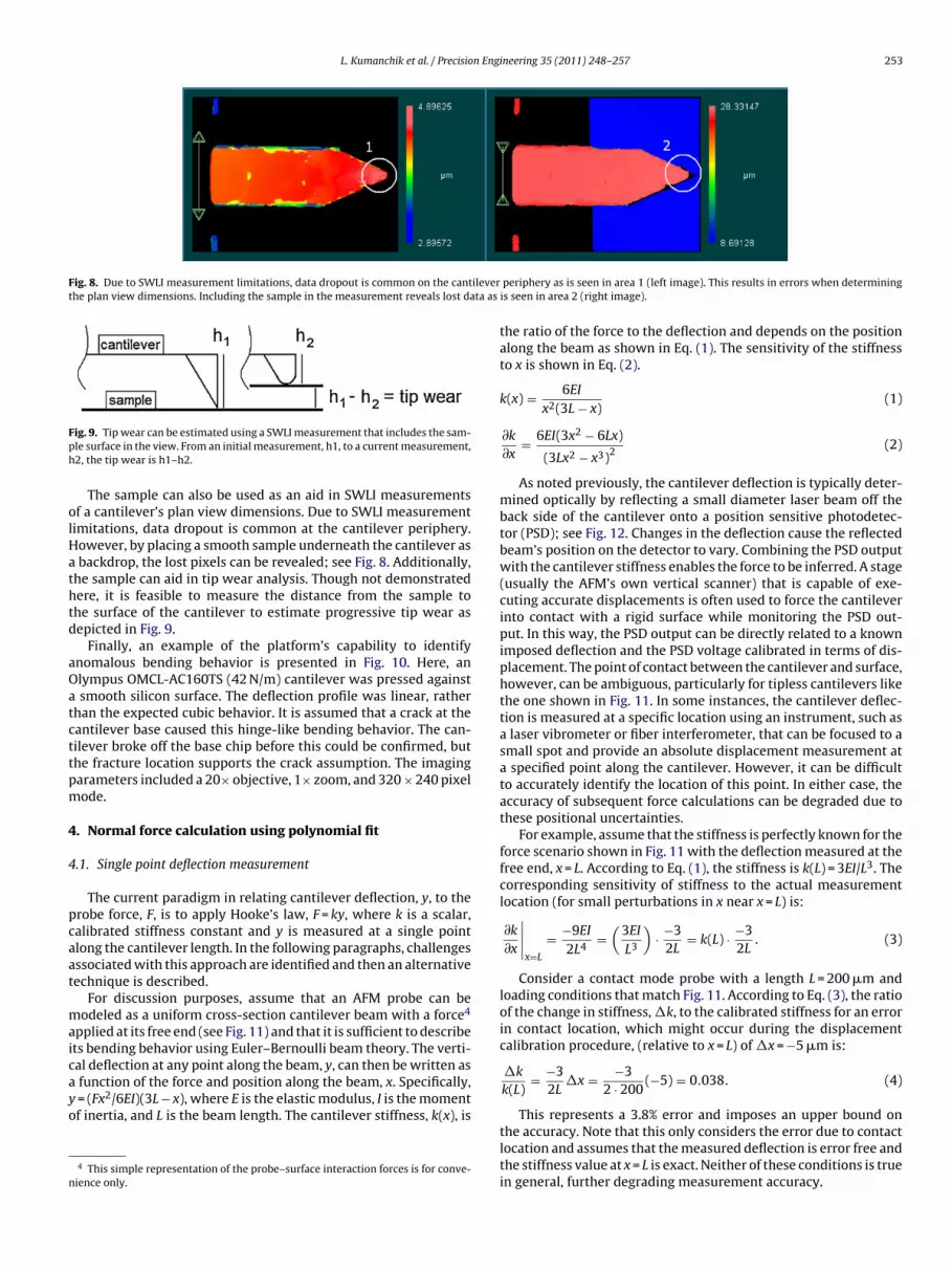
Fig. 8. Due to SWLI measurement limitations, data dropout is common on the cantileverthe plan view dimensions. Including the sample in the measurement reveals lost data as

Fph

olHathtd

aOatcttpm

4

4

pcaat

maicayo

n

ig. 9. Tip wear can be estimated using a SWLI measurement that includes the sam-le surface in the view. From an initial measurement, h1, to a current measurement,2, the tip wear is h1–h2.

The sample can also be used as an aid in SWLI measurementsf a cantilever’s plan view dimensions. Due to SWLI measurementimitations, data dropout is common at the cantilever periphery.owever, by placing a smooth sample underneath the cantilever asbackdrop, the lost pixels can be revealed; see Fig. 8. Additionally,

he sample can aid in tip wear analysis. Though not demonstratedere, it is feasible to measure the distance from the sample tohe surface of the cantilever to estimate progressive tip wear asepicted in Fig. 9.

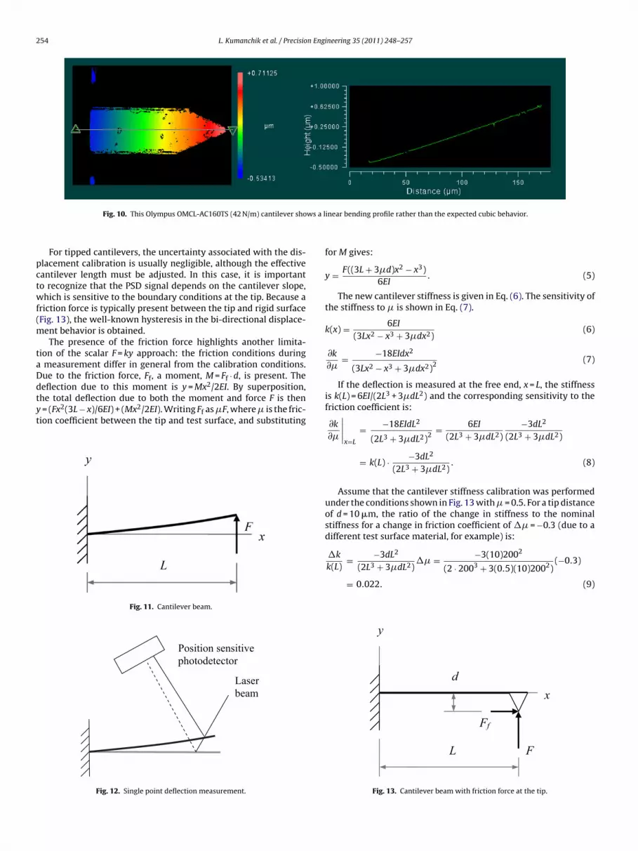
Finally, an example of the platform’s capability to identifynomalous bending behavior is presented in Fig. 10. Here, anlympus OMCL-AC160TS (42 N/m) cantilever was pressed againstsmooth silicon surface. The deflection profile was linear, rather

han the expected cubic behavior. It is assumed that a crack at theantilever base caused this hinge-like bending behavior. The can-ilever broke off the base chip before this could be confirmed, buthe fracture location supports the crack assumption. The imagingarameters included a 20× objective, 1× zoom, and 320 × 240 pixelode.

. Normal force calculation using polynomial fit

.1. Single point deflection measurement

The current paradigm in relating cantilever deflection, y, to therobe force, F, is to apply Hooke’s law, F = ky, where k is a scalar,alibrated stiffness constant and y is measured at a single pointlong the cantilever length. In the following paragraphs, challengesssociated with this approach are identified and then an alternativeechnique is described.

For discussion purposes, assume that an AFM probe can beodeled as a uniform cross-section cantilever beam with a force4

pplied at its free end (see Fig. 11) and that it is sufficient to describets bending behavior using Euler–Bernoulli beam theory. The verti-

al deflection at any point along the beam, y, can then be written asfunction of the force and position along the beam, x. Specifically,= (Fx2/6EI)(3L − x), where E is the elastic modulus, I is the momentf inertia, and L is the beam length. The cantilever stiffness, k(x), is

4 This simple representation of the probe–surface interaction forces is for conve-ience only.

periphery as is seen in area 1 (left image). This results in errors when determiningis seen in area 2 (right image).

the ratio of the force to the deflection and depends on the positionalong the beam as shown in Eq. (1). The sensitivity of the stiffnessto x is shown in Eq. (2).

k(x) = 6EI

x2(3L − x)(1)

∂k

∂x= 6EI(3x2 − 6Lx)

(3Lx2 − x3)2(2)

As noted previously, the cantilever deflection is typically deter-mined optically by reflecting a small diameter laser beam off theback side of the cantilever onto a position sensitive photodetec-tor (PSD); see Fig. 12. Changes in the deflection cause the reflectedbeam’s position on the detector to vary. Combining the PSD outputwith the cantilever stiffness enables the force to be inferred. A stage(usually the AFM’s own vertical scanner) that is capable of exe-cuting accurate displacements is often used to force the cantileverinto contact with a rigid surface while monitoring the PSD out-put. In this way, the PSD output can be directly related to a knownimposed deflection and the PSD voltage calibrated in terms of dis-placement. The point of contact between the cantilever and surface,however, can be ambiguous, particularly for tipless cantilevers likethe one shown in Fig. 11. In some instances, the cantilever deflec-tion is measured at a specific location using an instrument, such asa laser vibrometer or fiber interferometer, that can be focused to asmall spot and provide an absolute displacement measurement ata specified point along the cantilever. However, it can be difficultto accurately identify the location of this point. In either case, theaccuracy of subsequent force calculations can be degraded due tothese positional uncertainties.

For example, assume that the stiffness is perfectly known for theforce scenario shown in Fig. 11 with the deflection measured at thefree end, x = L. According to Eq. (1), the stiffness is k(L) = 3EI/L3. Thecorresponding sensitivity of stiffness to the actual measurementlocation (for small perturbations in x near x = L) is:

∂k

∂x

∣∣∣∣x=L

= −9EI

2L4=

(3EI

L3

)· −3

2L= k(L) · −3

2L. (3)

Consider a contact mode probe with a length L = 200 �m andloading conditions that match Fig. 11. According to Eq. (3), the ratioof the change in stiffness, �k, to the calibrated stiffness for an errorin contact location, which might occur during the displacementcalibration procedure, (relative to x = L) of �x = −5 �m is:

�k

k(L)= −3

2L�x = −3

2 · 200(−5) = 0.038. (4)

This represents a 3.8% error and imposes an upper bound onthe accuracy. Note that this only considers the error due to contactlocation and assumes that the measured deflection is error free andthe stiffness value at x = L is exact. Neither of these conditions is truein general, further degrading measurement accuracy.

254 L. Kumanchik et al. / Precision Engineering 35 (2011) 248–257

ws a l

pctwf(m

taDdtyt

Fig. 10. This Olympus OMCL-AC160TS (42 N/m) cantilever sho

For tipped cantilevers, the uncertainty associated with the dis-lacement calibration is usually negligible, although the effectiveantilever length must be adjusted. In this case, it is importanto recognize that the PSD signal depends on the cantilever slope,hich is sensitive to the boundary conditions at the tip. Because a

riction force is typically present between the tip and rigid surfaceFig. 13), the well-known hysteresis in the bi-directional displace-

ent behavior is obtained.The presence of the friction force highlights another limita-

ion of the scalar F = ky approach: the friction conditions duringmeasurement differ in general from the calibration conditions.ue to the friction force, Ff, a moment, M = Ff · d, is present. Theeflection due to this moment is y = Mx2/2EI. By superposition,

he total deflection due to both the moment and force F is then= (Fx2(3L − x)/6EI) + (Mx2/2EI). Writing Ff as �F, where � is the fric-

ion coefficient between the tip and test surface, and substituting

Fig. 11. Cantilever beam.

Laser

beam

Position sensitive

photodetector

Fig. 12. Single point deflection measurement.

inear bending profile rather than the expected cubic behavior.

for M gives:

y = F((3L + 3�d)x2 − x3)6EI

. (5)

The new cantilever stiffness is given in Eq. (6). The sensitivity ofthe stiffness to � is shown in Eq. (7).

k(x) = 6EI

(3Lx2 − x3 + 3�dx2)(6)

∂k

∂�= −18EIdx2

(3Lx2 − x3 + 3�dx2)2(7)

If the deflection is measured at the free end, x = L, the stiffnessis k(L) = 6EI/(2L3 + 3�dL2) and the corresponding sensitivity to thefriction coefficient is:

∂k

∂�

∣∣∣∣x=L

= −18EIdL2

(2L3 + 3�dL2)2= 6EI

(2L3 + 3�dL2)−3dL2

(2L3 + 3�dL2)

= k(L) · −3dL2

(2L3 + 3�dL2). (8)

Assume that the cantilever stiffness calibration was performedunder the conditions shown in Fig. 13 with � = 0.5. For a tip distanceof d = 10 �m, the ratio of the change in stiffness to the nominalstiffness for a change in friction coefficient of �� = −0.3 (due to adifferent test surface material, for example) is:

2 2

�k

k(L)= −3dL

(2L3 + 3�dL2)�� = −3(10)200

(2 · 2003 + 3(0.5)(10)2002)(−0.3)

= 0.022. (9)

x

FL

y

Ff

d

Fig. 13. Cantilever beam with friction force at the tip.

n Engineering 35 (2011) 248–257 255

acaawatm

dtao

4

Fib

y

wfpfid

F

�

tbd(Eb

wcbttsTftl

4

biadwtwl

2.12 mm field of view and 4.4 �m/pixel lateral resolution. The can-tilever was then laterally positioned under the objective using themotorized stage. The cantilever was longer than the field of viewso only a section of the cantilever was measured; stitching was

L. Kumanchik et al. / Precisio

Again, this 2.2% error places an upper bound on the achievableccuracy. As before, this analysis only considers the error due tohanges in friction coefficient between the tip and test surface andssumes that the measured deflection and calibrated stiffness valuere error free. Additionally, it does not incorporate the error thatould be obtained if the stiffness calibration was performed bydifferent method (e.g., vibration analysis or mass loading) such

hat the force conditions during calibration differed from the actualeasurement situation.The previous discussion highlights the limitations in single point

eflection measurements for AFM force determination. An alterna-ive to the traditional approaches for stiffness calibration that takesdvantage of the deflection profile made available by the interfer-metric measurement platform is described next.

.2. Full-field deflection measurement

Returning to the simple two-dimensional analysis shown inig. 11, assume that the full deflection profile, y(x), for the cantilevers measured during loading. As shown in Eq. (5), the deflection cane described by a third order polynomial:

(x) = 0 + 0x + F(3L + 3�d)6EI

x2 − F

6EIx3 = c0 + c1x + c2x2 + c3x3,

(10)

here the c0 and c1 coefficients are nominally zero. Given theull-field measurement, y(x), the least-squares solution for theolynomial coefficients may be calculated. Using only these coef-cients, the force and friction coefficient can then be uniquelyetermined by Eqs. (11) and (12).

= −6c3EI (11)

= −(3c3L + c2)3c3d

(12)

Eq. (11) is interesting because it requires little information abouthe beam. It applies regardless of the load application point, theeam stiffness, or the beam length. All that is necessary is a physicalescription of the beam’s cross-section and the material propertiesalthough obtaining these can sometimes still impose difficulties).q. (11) follows from the definition of shear, V, in an Euler–Bernoullieam:

d3y

dx3= −V

EI= −F

EI, (13)

hich remains constant along the beam length for any boundaryondition. By extension, the shear force in a beam of any shape cane determined from a multipoint measurement over a section ofhe beam as long as that section follows the assumptions that ledo Eq. (11). This applies, for example, to triangular shaped beamsince each leg may be considered to be an Euler–Bernoulli beam.he complete force vector can be determined using c2 to find theriction force component, but this requires more information abouthe beam. This paper focuses on the application of Eq. (11) andeaves Eq. (12) for future research.

.3. Experimental results for polynomial fit method

Eq. (11) was evaluated for the case of a mesoscale horizontaleam (no tip) with a vertical mass-based load applied (i.e., F was

deally the only force component). The beam was fabricated from50.8 mm diameter, double-sided polished 〈1 1 1〉 silicon wafer by

iamond cutting at the flat. The design dimensions for the beamere 1 mm wide, 5 mm long, and 0.3 mm thick. After fabrication,

he dimensions were measured using the SWLI. The average widthas 0.941 mm and the length was 4.820 mm (the SWLI lateral reso-

ution was 4.4 �m for a 5× objective at 0.5× zoom with a 640 × 480

Fig. 14. SWLI image of the fabricated cantilever. The enlarged field of view wasenabled by stitching multiple images together. It is seen that the width of the beamvaries slightly along its length. The wafer edge roll-off is observed at the free end(left end) of the beam.

detector). A thickness measurement was completed by placing aglass surface beneath the cantilever and using the SWLI to mea-sure the distance from the top of the glass surface to the top ofthe cantilever. The thickness value, t, was 0.305 mm (based onthe system noise floor of 2.7 nm, the uncertainty in t is at least±3 nm). A stitched SWLI image of the entire cantilever is shown inFig. 14.

The vertical loads for the beam were produced using a series of10 masses (Fig. 15); the individual masses were each suspendedfrom a tether which was looped over the beam (Fig. 16). The massvalues, m, were measured using a Mettler Toledo AB265-S/FACTprecision balance (0.1 mg resolution). The beam was fixed to aholder using CrystalbondTM heat-activated adhesive and the holderwas bolted to the tip-tilt stage.

The full-field measurement procedure was initiated by align-ing the cantilever base to the SWLI optical axis (the optical axiswas treated as parallel to the gravity vector, although the degreeof alignment was not determined). To perform this alignment, a5× objective with 0.5× zoom was applied to give a 2.82 mm by

Fig. 15. Masses used for vertical loading experiments.

256 L. Kumanchik et al. / Precision Engineering 35 (2011) 248–257

Fe

nc

1234

dlsftrsdrmhs

bmpF

wIitEucvsomFos(e

sary to consider the non-constant beam width and correspondingvariation in the moment of inertia along the beam’s axis. This wasaccomplished using the average widths, wavg, of the beam for thetwo selected fields of view. The result was evaluated by rearrang-

ig. 16. The cantilever was attached to the tip-tilt stage and loaded near the freend. Measurements are valid at any section between the base and the load point.

ot applied for the force measurements. The following steps wereompleted for each mass.

. Attach the mass to the cantilever;

. complete a first SWLI measurement;

. remove the mass; and

. complete a second SWLI measurement.

The two SWLI measurements were differenced to isolate theeflection caused by loading. As described before, differencing iso-

ates the deformation caused by mass loading from other sourcesuch as deformations caused by gravity loading. However, dif-erencing requires lateral alignment between images. Therefore,he mass was applied first in the measurement sequence since itequired the longest setup time. This reduced the time betweentep 2 and 4 to a few seconds, which mitigated the effect of lateralrift due to stage settling and thermal effects. In addition to drift-elated lateral motion, vertical deflection of the cantilever from theass loading also leads to a small shift (foreshortening) of the SWLI

eight map along the beam axis. Because the beam deflections weremall in this study, this shear effect was neglected.

A deflection profile was obtained for each mass loading resulty taking a section view through the beam center in the differenceap. The data was then fit in a least-squares sense using a cubic

olynomial to obtain the coefficient c3. Eq. (11) was rearranged andwas replaced by mg (g = 9.8 m/s2) to assist in the data analysis:

c3

m= −9.8

6E〈1 1 1〉I= C, (14)

here the applied mass is expressed in grams, E〈1 1 1〉 = 188 GPa [33],= wt3/12 for the rectangular cross-section, t = 0.305 mm, and C is

deally a constant. There was a noticeable taper in the width, w, sohe average value within the measurement field of view was used.q. (14) was evaluated as follows: (1) the left side was calculatedsing the measured values of c3 and mass; (2) the right side was cal-ulated based on the beam’s physical description; and (3) the twoalues were compared. Ideally, they should agree within the mea-urement uncertainty. The uncertainty in c3 was estimated basedn 11 trials per each of the 10 weights. The standard deviation wasultiplied by a coverage factor of 2. The results are displayed in

ig. 17. As seen in the figure, there is a small offset between theverall mean c3/m value (left hand side of Eq. (14)) and the con-tant evaluated from the beam properties (right hand side of Eq.14)). This difference is 0.4% and falls within the bounds set by therror bars.

Fig. 17. Estimates of the Eq. (14) expressions for 10 masses. The error bars are basedon a coverage factor of 2.

The variability of c3 with profile location in a single measure-ment was also investigated. Eleven deflection profiles near thebeam centerline were selected from a single image and used to indi-vidually calculate c3. The standard deviation was found to be 0.5%of the mean value. This deviation is an indicator of the model lim-its since the Euler–Bernoulli equations describe a two-dimensionalbeam; non-ideal loading conditions which imposed a slight twist tothe beam about its axis would cause the profile to vary with loca-tion, for example. Noise in the SWLI height map from the singlemeasurement result would also contribute.

Next, the cantilever was loaded and 11 separate measurementswere sequentially completed before removing the load. Only thecenterline profile was extracted from each measurement and wasused to calculate c3. The standard deviation was found to be 1.5%of the mean. This provides an indication of the limit imposed bythe environmental noise over the required measurement time ofapproximately 4 minutes.

Ideally, the force calculated using Eq. (11) is independent of themeasurement location for constant loading conditions. To test thisbehavior, a measurement (denoted 1) was completed for a field ofview near the free end and compared to a measurement (denoted 2)completed near the base; see Fig. 18. The values of c3 differed, how-ever, due to the variable beam width along its length (see Fig. 14).To enable a direct comparison of the two results, it was neces-

Fig. 18. A beam was loaded under identical conditions, but the measurement fieldof view was varied. The boxes represent the partially overlapping measurementregions along the beam’s axis. For identical loading, the shear should be identicalregardless of location.

n Eng

imA

wd((ta

n(kwfcvF .BpoFaf1

5

fgphsUoofpamwbptataw

A

Soa

R

[

[

[

[

[

[

[

[

[

[

[

[

[

[

[[

[

[

[

[

[

[

Review of Scientific Instruments 2007;78:093705.

L. Kumanchik et al. / Precisio

ng Eq. (11), substituting for I, and considering the ratio of the twoeasurement results 1 and 2 (same mass, but different location).fter simplification, the ratio is:

(−6c3E〈1 1 1〉I/mg)1(−6c3E〈1 1 1〉I/mg)2

= (−6c3E〈1 1 1〉wavgt3/12mg)1

(−6c3E〈1 1 1〉wavgt3/12mg)2= (c3wavg)1

(c3wavg)2= 1,

(15)

hich is nominally equal to 1. Experimentally, the ratio wasetermined to be 1.03 based on the following values: m = 8.617 g,c3)1 = −37.02 m−2, (wavg)1 = 0.88 mm, (c3)2 = −33.89 m−2, andwavg)2 = 0.93 mm. This deviation from unity is reasonable givenhe 1.5% standard deviation obtained from the repeated c3 tests forsingle load with the profile extracted along the beam’s centerline.

In a second study of the polynomial fit-based force determi-ation approach, a horizontal Olympus OMCL-AC240TS proberectangular cross-section, 30 �m × 2.8 �m, 240 �m length,= 1.8 N/m, ∼14 �m tip height, less than 10 nm tip radius)as deflected vertically against a rigid, smooth silicon sur-

ace. The experimental c3 value was −2.11 × 104 m−2 from theenterline deflection profile. If the manufacturer-specified EIalue of 8.29 × 10−12 N-m2 is applied, the resulting vertical force is= − 6c3EI = − 6( − 2.11 × 104)8.31 × 10−12 = 1.05 × 10−6 N = 1.05 �Nased on the measured deflection of 0.59 �m at therobe’s free end (from the SWLI height map), the forcebtained from the manufacturer’s spring constant is= 1.8(0.59 × 10−6) = 1.06 × 10−6 N = 1.06 �N. This gives a 1%greement and provides a preliminary validation of the methodor a typical AFM probe. Data was collected using a 20× objective,x zoom, 320 × 240 pixel detector.

. Conclusions

In this paper, an interferometric platform for measuring theull-field deflection of atomic force microscope (AFM) probes andeneric cantilevers during quasi-static loading was presented. Thelatform consists of a scanning white light interferometer (SWLI),olders for the cantilevers, a translation stage, a rotation (tip-tilt)tage, and an adapter plate to connect these units to the SWLI table.sing the platform, studies were completed to enable visualizationf cantilever behavior for snap-in against a rigid surface, cantilever-n-cantilever bending tests, and the anomalous bending profileor a damaged AFM probe. Additionally, the full-field deflectionrofiles measured by the platform were used to establish a newpproach for normal force calculation. In this method, a polyno-ial fit to the cantilever deflection profile was used, in conjunctionith the elastic modulus and area moment of inertia for the test

eam, to estimate the normal force. Experimental validation wasrovided. Future efforts in this research will include: (1) expandinghe analysis to a surface fit, rather than a line fit to the SWLI datas presented here; (2) extension of the approach to include the full,hree-dimensional force vector at the probe tip; (3) completion ofn uncertainty analysis; and (4) an evaluation of the effects of tipear on measured force.

cknowledgements

This work was partially supported by the National Institute oftandards and Technology. Any opinions, findings, and conclusionsr recommendations expressed in this material are those of theuthors and do not necessarily reflect the views of this agency.

eferences

[1] Binnig G, Quate CF, Gerber C. Atomic force microscope. Physical Review Letters1986;56:930–3.

[

[

ineering 35 (2011) 248–257 257

[2] Shenkenberg, D., Boldly going where no one has gone before, Photonics Spectra,December, 2008, pp. 68–71.

[3] Thundat T, Chen GY, Warmack RJ, Allison DP, Wachter EA. Vapor detec-tion using resonating microcantilevers. Analytical Chemistry 1995;67/3:519–21.

[4] Vettiger P, Cross G, Despont M, Drechsler U, Durig U, Gotsmann B, et al. The“millipede”–nanotechnology entering data storage. IEEE Transactions on Nan-otechnology 2002;1/1:39–55.

[5] Cumpson P, Zhdan P, Hedley J. Calibration of AFM cantilever stiffness: amicrofabricated array of reflective springs. Ultramicroscopy 2004;100:241–51.

[6] Cleveland J, Manne S, Bocek D, Hansma P. A nondestructive method for deter-mining the spring constant of cantilevers for scanning force microscopy.Review of Scientific Instruments 1993;64/7:1868–73.

[7] Butt HJ, Siedle P, Seifert K, Fendler K, Seeger T, Bamberg E, et al. Scan speedlimit in atomic force microscopy. Journal of Microscopy 1993;169:75–84.

[8] Hutter J, Bechhoefer J. Calibration of atomic-force microscope tips. Review ofScientific Instruments 1993;64/7:1868–73.

[9] Li Y, Tao N, Pan J, Garcia A, Lindsay S. Direct measurement of interaction forcesbetween colloidal particles using the scanning force microscope. Langmuir1993;9/3:637–41.

10] Neumeister JM, Ducker WA. Lateral, normal, and longitudinal spring con-stants of atomic force microscopy cantilevers. Review of Scientific Instruments1994;65/8:2527–31.

11] Senden T, Ducker W. Experimental determination of spring constants in atomicforce microscopy. Langmuir 1994;10/4:1003–4.

12] Smith S, Howard L. A precision, low-force balance and its application toatomic force microscope probe calibration. Review of Scientific Instruments1994;65/4:903–9.

13] Sader J, Larson I, Mulvaney P, White L. Method for the calibration of atomic forcemicroscope cantilevers. Review of Scientific Instruments 1995;66/7:3789–98.

14] Sader J. Parallel beam approximation for V-shaped atomic force microscopecantilevers. Review of Scientific Instruments 1995;66/9:4583–7.

15] Gibson CT, Watson GS, Myhra S. Determination of the spring constants of probesfor force microscopy/spectroscopy. Nanotechnology 1996;7:259–62.

16] Myhra S. In: Riviere JC, Myhra S, editors. Handbook of Surface and Inter-face Analysis Methods for Problem Solving. New York: Marcel Dekker; 1998.p. 52.

17] Sader J, Chon J, Mulvaney P. Calibration of rectangular atomic force microscopecantilevers. Review of Scientific Instruments 1999;70/10:3967–9.

18] Levy R, Maaloum M. Measuring the spring constant of atomic force micro-scope cantilevers: thermal fluctuations and other methods. Nanotechnology2002;13:33–7.

19] Gibson C, Weeks B, Abell C, Rayment T, Myhra S. Calibration of AFM cantileverspring constants. Ultramicroscopy 2003;97:113–8.

20] Ogletree D, Carpick R, Salmeron M. Calibration of frictional forces inatomic force microscopy. Review of Scientific Instruments 1996;67/9:3298–306.

21] Bogdanovic G, Meurk A, Rutand MW. Tip friction–torsional spring con-stant determination. Colloids and Surfaces B: Biointerfaces 2000;19:397–405.

22] Green CP, Lioe H, Cleveland JP, Proksch R, Mulvaney P, Sader JE. Normal andtorsional spring constants of atomic force microscope cantilevers. Review ofScientific Instruments 2004;75/6:1988–96.

23] Cannara R, Eglin M, Carpick R. Lateral force calibration in atomic forcemicroscopy: a new lateral force calibration method and general guidelines foroptimization. Review of Scientific Instruments 2006;77/5:053701.

24] http://www.nist.gov/mel/mmd/mf/sfmet.cfm.25] Jabbour Z, Yaniv S. The kilogram and measurements of mass and force.

Journal of Research of the National Institute of Standards and Technology2001;106:25–46.

26] Newell D, Kramar J, Pratt J, Smith D, Williams E. The NIST microforce real-ization and measurement project. IEEE Transactions of Instrumentation andMeasurement 2003;4:158–61.

27] Pratt J, Smith D, Newell D, Kramar J, Whitenton E. Progress toward SystèmInternational d’Unités traceable force metrology for nanomechanics. Journal ofMaterials Research 2004;19:1.

28] Pratt J, Kramar J, Newell D, Smith D. Review of SI traceable force metrology forinstrumented indentation and atomic force microscopy. Measurement Scienceand Technology 2005;16:2129–37.

29] Gates R, Pratt J. Prototype cantilevers for SI-traceable nanonewton force cali-bration. Measurement Science and Technology 2006;17:2852–60.

30] Pratt J, Kramar J, Shaw G, Smith D, Moreland J. A peizoresistive cantilever forcesensor for direct AFM force calibration. Materials Research Society SymposiumProceedings 2007;1021:HH02–03.

31] Langlois E, Shaw G, Kramar J, Pratt J, Hurley D. Spring constant calibrationof atomic force microscopy cantilevers with a piezosensor transfer standard.

32] Niehues J, Lehmann P, Bobey K. Dual-wavelength vertical scanninglow-coherence interferometric microscope. Applied Optics 2007;46/29:7141–8.

33] McSkimin H, Andreatch Jr P. Measurement of third-order moduli of silicon andgermanium. Applied Physics 1964;35/11:3312–9.