Embed Size (px)
Citation preview

An Investigation of Stock Market Anomalies: the Weekend Effect
by
Dennis Olson School of Business and Management
American University of Sharjah Sharjah, United Arab Emirates
Nan-Ting Chou Department of Economics University of Louisville
Louisville, Kentucky, USA [email protected]
Charles Mossman
Department of Accounting and Finance I.H. Asper School of Business
University of Manitoba Winnipeg, Manitoba, Canada [email protected]
JEL: B3 Correspondence Address: Nan-Ting Chou Economics Department School of Business University of Louisville Louisville, Kentucky, USA [email protected]

An Investigation of Stock Market Anomalies: the Weekend Effect
Abstract There are several well-known stock market anomalies: the weekend effect, turn-of-the-
month effect, and January effect. This paper investigates the evolution of the weekend
effect and hypothesizes a life cycle for this stock market anomaly involving identification,
exploitation, decline, reversal, and finally disappearance. Data for seven U.S. stock indices
for 1973 – 2005 suggest that the weekend effect may have already gone through this entire
cycle. The negative weekend effect declined first for large stocks and now has mostly
disappeared even for small stocks. The reverse weekend effect that was identified in large
stocks in the 1990s has similarly declined in recent years. Across all stock indexes, the
weekend effect appears to be in the last stage of its cycle—disappearance.
JEL Classification: B3
Key Words: Anomalies, weekend effect, day-of-the-week, life cycle
1

An Investigation of Stock Market Anomalies: the Weekend Effect
1. Introduction
Seasonal anomalies--such as the weekend effect, turn-of-the-month effect, and
January effect--have been well documented in the finance literature. Although the
existence of negative abnormal returns on Mondays or positive abnormal returns around the
turn of the month or year does not contradict market efficiency, once discovered, the
seasonalities should be eliminated if they are large enough to be profitably exploited.
Studies such as Harris (1986), Kim (1988), and Chow, Hsiao, and Solt (1997) have pointed
out strategies that investors could use to capitalize on the weekend effect. Haugen (1988)
has written a book for the popular press showing how to take advantage of the January
effect, and recently Hensel and Ziemba (1996) have shown how an investor could
profitably exploit the turn-of-the-month (TOM) anomaly.
In reasonably efficient markets, stock market anomalies should be eliminated soon
after their discovery if the inefficiency is large enough to be profitably exploited. Dimson
and Marsh (1999, p.1) note that “once an anomaly is publicized, only too often it disappears
or goes into reverse.” As an example, Vergin and McGinnis (1999) and Keef and Roush
(2005) have shown that positive excess returns on the day before holidays that were so
prevalent before 1987 diminished substantially in the 1990s. Chong, Hudson, Keasey, and
Littler (2005) further document that pre-holiday returns in the U.S., U.K., and Hong Kong
markets reversed or turned negative over the period 1991-1997 and effectively disappeared
in the period 1997-2003. Similarly, Gu (2003) has reported a declining January effect in
2
U.S. equity markets following the stock market crash of 1987. Singal (2004) examined 10
anomalies and concluded that their magnitudes have either diminished over time, or that
significant transaction costs and/or risk prevent the market from totally eliminating these
mispricings.
The January effect, as first identified by Rozeff and Kinney (1976), is the tendency
for stocks to have larger returns in January than in other months of the year. It has since
been strongly related to returns on small capitalization stocks. For example, Keim (1983)
found that the small firm premium, which is the differential return between small and large
stocks was .714% per day in January from 1963-1979. More recently, Haugen and Jorion
(1997) have shown that the January effect continues to persist into the decade of the 1990s.
The turn-of-the-month effect was the last of the three major seasonal anomalies to
be identified in the finance literature. Ariel (1987) brought the turn-of-the-month (TOM)
effect to the attention of the financial community. He showed that virtually all of the annual
return on U.S. stock indices occurs on the first 10 trading days of the month and that most
of this return occurs on the last trading day of the month and the first three or four days of
the next month. Depending upon the index used and the time period of analysis, the
average daily return during TOM days is .1% to .2% larger than on other trading days.
We investigate the weekend effect involving negative returns on Mondays (after the
weekend) and hypothesize a life cycle for this stock market anomaly. The weekend effect
was first identified by Cross (1973) and more formal investigation by French (1980) and
Gibbons and Hess (1981) documented day of the week regularities involving above
average Wednesday and Friday returns and significantly negative Monday returns of -
3

.1% to -.2% for U.S. stocks.1 However, soon after public recognition of the weekend
effect, Rogalski (1984) and Connolly (1989) showed that it was unstable over time and that
it had declined in significance by the early 1980s. More recently, Brusa, Liu, and Shulman
(2000, 2003, 2005) , Mehdian and Perry (2001), and Gu (2004) report that the negative
weekend effect has reversed and become a positive Monday effect following the stock
market crash of 1987. Since this “reverse weekend effect” is a new anomaly, we expect that
it will also decline in importance now that it has been formally identified.
We suggest that this pattern of changes in the weekend effect can perhaps be
explained by a five-stage life cycle as follows. (1) The cycle begins when someone
uncovers a non-random pattern in returns and either discloses it, or begins to exploit it.
(2) Other investors notice the anomaly and profits decline due to competition among
investors. As this happens, some investors who were profiting from the anomaly feel
they have more to gain from the publicity of revealing how they successfully exploited it.
At about the same time finance professors publish information about the existence of the
anomaly along with various explanations of its cause. The anomaly then nearly
disappears. (3) Once sophisticated investors believe that the anomaly is public
knowledge, they ignore it and it often reappears or even intensifies in magnitude.2 (4)
Then, someone rediscovers the anomaly and publicizes its renewed existence. With so
many investors focusing on the anomaly, they simultaneously try to exploit it—unaware
of the concurrent actions of others. The combined activity of all investors may lead to
over reaction and a temporary reversal of the anomaly. (5) Finally, after all adjustments
occur, both the anomaly and the reverse anomaly disappear.
4

This paper investigates the behavior of the weekend effect and explores the existence
of its life cycle in the U.S. stock market. We examine the dynamics of the weekend over
time and conduct Chow and Bai-Perron breakpoint tests to determine the stability of the
weekend effect. Our results indicate that there have been several different regimes for large
and small stocks over the period 1973-2005. The weekend effect has declined, intensified,
declined once again, and has generally disappeared in recent years. For large stocks, this
adjustment process produced a reverse weekend effect in the 1990s that seems to have
disappeared soon after its identification in the finance literature in 2000. The negative
weekend effect in small stocks has persisted longer, but does not appear to be present after
mid 2003. Our results indicate that the weekend effect has gone through a full life cycle.
2. Literature Review
Since pointed out by Cross (1973), the weekend effect involving negative returns to
stocks between Friday's close and Monday's close has been extensively analyzed in the
finance literature. Beginning with French (1980) and Gibbons and Hess (1981), several
studies have since documented day of the week regularities in U.S. stocks. That is, Monday
returns have been significantly negative and Wednesday and Friday returns have been
significantly positive. Lakonishok and Smidt (1998) showed that seasonal effects have been
persistent in U.S. returns for over ninety years and Jaffe and Westerfield (1985) showed that
the weekend effect has been present in several countries other than the U.S.
Numerous theories have been advanced to explain the weekend effect. Various
arguments involving measurement errors, behavior of specialists, payment delays in
settlement procedures, and daily patterns in the bid-ask spread have been examined and
5

rejected by Keim and Stambaugh (1984), Rogalski (1984), and Jacobs and Levy (1988).
Jacobs and Levy (1988) advanced the negative information flow hypothesis that suggests
that negative Monday returns are caused by firms delaying the release of bad news until
the weekend. However, Schatzberg and Datta (1992) and Pettengill and Buster (1994)
indicated that firms are more likely to announce good news over the weekend than bad
news. The most plausible remaining explanations for the weekend effect involve
differential day-of-the-week behavior by individual investors or by institutional
investors.
Miller (1988) hypothesized that individual investors tend to sell stock on Monday
and cause the weekend effect. They buy stocks throughout the week following broker
recommendations, but make sell decisions on their own after reviewing their portfolios
on weekends. Hence, individual investors tend to sell stocks on Mondays. Lakonishok
and Maberly (1990) provided empirical support for Miller’s hypothesis by showing that
individual investors trade more on Mondays and their ratio of sell to buy orders is higher
on Mondays than on other days of the week. If this hypothesis were correct, we would
expect the weekend effect to be more prevalent for small stocks with little institutional
ownership than for large stocks owned by institutional investors.
Sias and Starks (1995) have shown that day-of-the-week patterns in volume and
returns are more pronounced for stocks with higher institutional ownership than for stocks
with lower institutional ownership. Institutional investors begin the week by reviewing
portfolios and are not as likely to trade on Monday mornings, so that a lack of
institutional buyers on Monday morning is responsible for the negative weekend effect.
6

Alternatively, Chan and Singal (2003) and Singal (2004) argue that short sellers (who are
primarily institutions) are reluctant to hold short positions over the weekend, so they buy
stocks on Fridays to close out their short positions. This buying pressure causes the
positive Friday effect, while the reinstatement of short positions on Mondays causes
prices to fall at the start of the week. Chan and Singal (2003) have shown that the full
weekend effect, which they define as Friday’s return minus Monday’s return, is larger for
stocks with greater short interest. If their hypothesis is correct, the weekend effect should
be more prevalent for large stocks than for the small stocks held primarily by individual
investors. Also, assuming institutional investors are more sophisticated and better able to
alter their behavior than individual investors, adjustment to the anomaly and its
subsequent decline should occur for large stocks sooner than for small stocks.
Rogalski (1984) and Connolly (1989) have shown that the weekend effect is
rather unstable over time and that it diminished in statistical significance relatively soon
after its formal identification in 1973. However, Wilson and Jones (1993) deemed these
proclamations premature, noting that a weekend effect was present from 1973 to 1991 on
all three major U.S. stock exchanges. Abraham and Ikenberry (1994) and Sias and Starks
(1995) also indicated that a weekend effect exists for U.S. stocks over various time
horizons of nine to twenty nine years over the period from 1963 to 1991. In contrast,
Kamara (1997) showed that the Monday seasonal in S&P 500 returns declined
significantly from 1962 to 1993, while it remained intact over the whole period for a
small-cap index of stocks. In an international setting, Steeley (2001) has shown that the
weekend effect has mostly disappeared in the UK for the FTSE index in the 1990s, while
7

Tan and Tat (1998) documented a lessening of all seasonal anomalies in the Singapore
market in the 1990s. In further exploring the timing of the weekend effect, Abraham and
Ikenberry (1994) found a strong positive autocorrelation effect meaning that negative
Monday returns generally only followed negative Friday returns, whereas Monday
returns were positive on average following positive Friday returns. Wang, Li, and
Erickson (1997) demonstrated another unique characteristic of the weekend effect--that
the negative Monday returns were most pronounced in the second half of each month and
not statistically significant in the first half of the month.
Consistent with the latter phases of our life cycle hypothesis, Brusa, Liu, and
Schulman (2000) reported that the weekend effect reversed during the period from1990-
1994. That is, Monday returns were the largest of any day of the week for the Dow-Jones
Industrial, CRSP Value-Weighted, Standard and Poor’s 500, and New York Composite
stock indices. Friday returns experienced a similar reversal, so that returns on that day
were the smallest of any day of the week. Mehdian and Perry (2001) subsequently
demonstrated that the reverse weekend effect was statistically significant for U.S. large
stocks from November 1987 to August 1998, but that a negative Monday effect was still
present for smaller stocks. They further showed using Chow breakpoint tests that
Monday returns were unstable over the 1964 – 1998 period, but stable during both the pre
and post-1987 subsamples. Such results confirm that the weekend effect for large stocks
has changed over time--from reliably negative pre-crash, to positive and stable in the
post-crash period from 1988 - 1998.
Several recent articles have investigated the details of the reverse weekend effect.
8

Brusa, Liu, and Schulman (2003) showed that the weekend and reverse weekend effects
exist in a broad range of industries and that the effects are similar across months of the
year. Brusa and Lui (2004) found that the positive Monday returns are concentrated in
the first and third weeks of each month, while Brusa, Lui, and Schulman (2005) shows
that the reverse weekend effect (like the weekend effect) is correlated with the previous
Friday return. Thus, positive Monday returns for large stocks are most likely to be
observed after Friday returns. Finally, Gu (2004) suggested that the weekend effect
became well-known in the late 1980s and that sophisticated investors subsequently over
exploited the effect leading to a reversal. Building upon this body of work, we suggest
that a life cycle explains the changing pattern in the weekend effect over time. The
adjustments reported in previous studies for the 1990s should be continuing. We would
expect more recent data to reveal that markets adjust. Therefore neither the weekend, nor
the reverse weekend effect should continue to be as strong as before.
3. Data and preliminary analysis
The primary data for this study are seven daily U.S. stock market index return series
for the period 1973 – 2005 obtained from Datastream. The series include the two most
widely followed indices--the Dow-Jones 30 Industrials (DOW) of very large capitalization
stocks and the Standard and Poor's 500 (SP500) index of large cap stocks. Medium
capitalization stocks are represented by returns of the Standard & Poor’s Midcap 400
(SPmid), while small stocks are represented by the Standard & Poor’s Smallcap 600
(SPsmall).3 To further explore the possibilities of differential effects across indices with
different sectoral weightings, we also obtained returns for the NASDAQ Composite, the
9

NASDAQ 100, and the American Stock Exchange (AMEX) Composite indices.4 Although
data for the DOW and S&P500 are available back to the 1920s, the time period of analysis
begins in 1973--the first year for which data are available for all seven of these indices.
For each index, daily compound percentage returns (Rt) are calculated from index
closing prices as Rt = 100*ln(It / It-1), where It is the closing level of the index and It-1 is the
closing value for the previous day. Since the stock market crash of October 1987 has been
identified by De Lima (1998, p. 227-228) as a highly influential event corresponding to a
regime shift in the distribution of stock returns, our analysis is performed excluding the
22 days of October 1987. This leaves 8310 daily observations—3627 for the pre-crash
period of 1972 - September 1987 and 4683 observations for November 1987 – 2005. The
post-crash period is further divided into the period from November 1987 to 2000 ( 3327
observations) which is the period of the known reverse weekend effect, and the years
2001 – 2005 (1256 observations) which is approximately the period that follows the
formal identification of the reverse weekend effect. These breakpoints are supported by
sequential Chow test and Bai-Perron test, which are discussed later.
Day-of-the-week effects on each of the seven indices are obtained by regressing
daily returns on day-of-the-week dummy variables as follows:
Rt = β1Mondayt + β2Tuesdayt + β3Wednesday + β4Thursdayt + β5Fridayt + εt, (1)
where Mondayt - Fridayt are day-of-the-week dummies, β1 - β5 are regression parameters
showing average daily returns, and εt is the error term. This regression is run without an
intercept to calculate the actual magnitude of returns on each day and it is performed
separately for each of the five market indices during both the pre-crash and post-crash
10

periods.
To determine if returns on Monday are significantly different from returns on other
days of the week, we run the following regression:
Rt = β0 + β1Mondayt + εt, (2)
where β1 represents the market return premium on Mondays (above the average for other
days), and β0 is a constant representing the average return for the other four days of the week.
If β1 is statistically different from zero, a weekend effect exists during the period of data
examined. Replacing the Monday dummy with dummies for other days of the week and re-
running the regression four times gives the significance of each day of the week relative to
the average return for the other four days.
Table 1 shows day of the week returns for the seven indices for the pre-crash period,
the post-crash known reverse anomaly period, and for the years following the identification
of the reverse weekend effect. Ordinary least squares regressions based on equation (1) are
adjusted for heteroskedasticity and the t-statistics are shown in parentheses beneath the mean
daily returns.5 An asterisk denotes daily returns that are statistically different from zero at
the 5% level of significance, while returns are boldfaced if they are statistically different
from returns on the other days of the week at the 5% level of significance. For the pre-crash
period in Panel A, Monday returns are negative for all five indices, ranging from -.064% for
the DOW up to -.210% for the NASDAQ. Returns are statistically different from zero at the
5% confidence level for all indices except the DOW, and even for the DOW, Monday
returns are significantly smaller than the mean return for other days of the week. This
illustrates the well-known weekend effect as shown in numerous studies. Wednesdays
11

provide the largest day of the week returns for the large stocks of the DOW, SP500 and
NASDAQ 100, while Fridays have the largest returns for small to mid size stocks. Tuesday
returns are rather small and the day-of-the-week pattern generally confirms results in
Gibbons and Hess (1981). Day-of-the-week effects are more pronounced for smaller stocks
(and for the NASDAQ100) than for larger stocks, as previously pointed out by Kamara
(1997).
Panel B of Table 1 presents average daily returns for the seven stock market indices
during the period of the known reverse weekend effect from November 1987 to 2000.
Monday returns are positive for the DOW, S&P 500, and for the NASDAQ 100 indices.
They are statistically significant at the 5% level for the DOW and the S&P 500 and larger
than for any other day of the week. For the DOW, Monday’s return is significantly larger
than the average return on the other days of the week. These results confirm the existence of
the reverse weekend effect in large stocks for the late 1980s and the decade of the 1990s.
The magnitude of the negative Monday returns and positive Friday returns declined
across all indices relative to the pre-crash time period. Thus, the full weekend effect defined
by Chan and Singal (2003) as Friday’s return minus Monday’s return declined
substantially from earlier years. The weekend effect still exists for small stocks from
1987-2000, but is smaller than in the pre-crash era.
Panel C of Table 1 shows returns for the period following the publication of articles
identifying the reverse weekend effect. Monday returns are almost zero for large stocks, so
the reverse weekend effect seems to have disappeared rather quickly after it was pointed out.
Monday returns for small stocks are also very close to zero, meaning that the negative
12

weekend effect has similarly disappeared in small stocks. Consistent with our life cycle
hypothesis, both institutional and individual investors appear to have altered behavior to
effectively eliminate all types of weekend effects. Strong differential day-of-the-week
effects now seem to exist only for the AMEX, NASDAQ, and NASDAQ100 indices. For
example, Friday returns are still statistically larger than on other days of the week for the
AMEX, while the NASDAQ and NASDAQ 100 have large positive Wednesday returns and
even larger negative returns on Fridays. Negative Friday return in NASDAQ stocks during
2001-2005 might appear to represent an anomaly, but the explanation is undoubtedly risk
related. During this period of high volatility, investors were hesitant to maintain holdings in
technology-related stocks of the NASDAQ over the weekend. This fear appears to have
caused a sell-off each Friday and a new temporary day-of-the-week effect that should
eventually be eliminated.
4. Changes in the weekend effect over time
Since daily return patterns are somewhat consistent across the large stock indices and
also fairly similar among the small to mid-size stock indices, further analysis focuses on just
two index return series. The DOW is considered representative of large stocks and the S&P
Small Cap 600 (SPsmall) is used as the small stock index.
Following Connolly (1989), the stability of the weekend effect based on both Friday
and Monday returns can be examined by four-year subperiods for the years 1973 – 2004.
Returns for Mondays and Fridays relative to other days of the week are estimated by
Rt = β0 + β1Mondayt + β2Fridayt + εt. (3)
Panel A of Table 2 shows the dynamics of Monday and Friday returns for large
13

stocks over time. Monday returns are negative, but not quite significant at the 5% level over
4-year periods from1973 to 1988. The reverse weekend effect appears in 1989-1992 and is
statistically significant for 1993-1996 and 1997-2000. In fact, the reverse weekend effect
intensifies for the years 1997-2000. For the years 2001-2005, Monday returns are smaller
than on other days of the week, but not significantly different from zero. Notice also that the
differential Friday return changes from positive to negative quite often between periods.
Differentially large Friday returns historically seen in many stock indices have generally not
been present in the return pattern for the Dow Jones industrials.
5. Graphical Representation of the Weekend Effect
The dynamics of the weekend effect probably are best seen by graphically
comparing Monday to the rest of the rest of the week. The power ratio developed by Gu
(2003, 2004) provides a nice way to illustrate differential Monday returns and a slight variant
of his power ratio can be developed from the following equations:
* (1 )FR Monday return= + (4)
* (1 )WR Average daily return onother days of the week= + . (5)
Returns are expressed as decimals and the Average daily return on other days of the week is
calculated for the four days preceding each Monday. If any of those days are a holiday, the
average daily return is calculated over three days.6 The power ratio for Monday’s return is
*
*M
MW
RPRR
= . (6)
The power ratio is always positive and is used to convert the daily data series into weekly
observations. The traditional negative weekend is present whenever PRM < 1 and the reverse
14

weekend effect exists if PRM > 0. The stability of the Monday effect can also be examined
using these weekly values.
To calculate the power ratio for the full weekend effect PRWE, we simply replace the
numerator of equation (6) with (1 + Friday’s return – Monday’s return) for each week. The
denominator for the average return for the rest of the week is calculated the same as in
equation (5), except that it contains one less day of returns. The interpretation is reversed
relative to PRM. Thus, PRWE > 0 shows the presence of the traditional full weekend effect.
Since there is considerable week to week fluctuation in the power ratio, smoothing
can be used to better illustrate trends. The tradeoff between seeing the big picture and
greater detail is perhaps best accomplished with a one to three year (52 to 156 week) moving
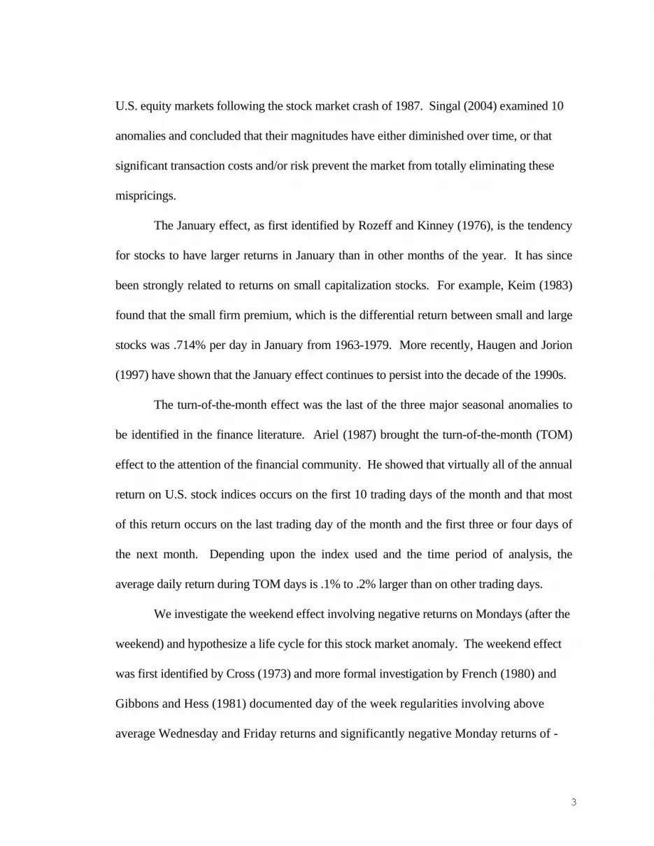
average of the weekly power ratio. Figure 1 shows the power ratio for smoothed Monday
returns (PRM) for the period 1973-2005 (excluding October of 1987). Panel A depicts results
for the Dow –Jones Industrials and Panel B shows the power ratio for S&P Small Cap 600.
The graphs are displayed by observation number and there are 1584 Monday returns over
this period.
Graphical results provide much better detail about the dynamics of the weekend
effect than dummy variables. In Panel A, the Monday power ratio for the DOW (smoothed
over one year, or 52 weeks) shows that the initial reaction to publication of information
about the existence of the negative Monday effect in 1973 led to a rapid increase in the
Monday power ratio. This means the negative Monday return declined and seemed to be
eliminated by about observation 175. However, smoothing is essentially a 52 week
centering of returns, so the initial local peak in the power ratio probably occurred about 26
15

weeks earlier, or around January of 1976. From this point the power ratio trends downward
as the anomaly intensifies. It reaches a local minimum between observations 400 and 450,
or in about March of 1981 when adjusted for centering. This was the peak of the negative
Monday effect for the Dow. From this point forward, Monday returns generally increased
over time and turned positive sometime between December of 1987 and July of 1988. The
reverse weekend effect then intensified until it reached a peak around observation 1360, or
about 1334 after adjusting for centering. This occurred in about October of 2000. Thus, the
zenith of the reverse weekend effect occurred just months after it was formally identified in
the finance literature. From 2001 onward, the reverse weekend effect quickly declined and a
small negative weekend effect returned for about a year. For 2004 and 2005, there is no
apparent weekend or reverse weekend effect in the DOW.
Panel B of Figure 1 illustrates the dynamics of the Monday effect for the S&P
SmallCap 600. Since this series is a bit noisier than the DOW, returns are smoothed over
three years (156 weeks) to provide better visual clarity. Like the DOW, the weekend effect
on small stocks declined and was essentially eliminated by about January of 1976. Then it
reappeared and the power ratio reached a global minimum in about April of 1981. Monday
returns then steadily increased until the weekend effect once again seems to disappear by
about September of 1990. Soon after, however, the negative weekend effect reappeared for
small stocks and even becomes more pronounced until about February of 2002. The
Monday power ratio reached a local minimum at this point and has generally increased
thereafter. Adjustments seem to have taken place so that there is no noticeable Monday
effect in small stocks in 2004 and 2005.
16

To further explore adjustments occurring with the weekend effect, Figure 2 shows
the power ratios for the full weekend effect for both large and small stocks over the period
1973-2005. Both Monday and Friday returns must be available for the full weekend effect
and this provides a data set of 1424 observations. Although it masks some of the
adjustments, a 3-year moving average of the power ratio is chosen to best depict the
dynamics of the full weekend effect. Once again, recall that PRWE > 1 represents the
traditional weekend effect and that PRWE < 1 shows the reverse full weekend effect.
For large stocks, the decline in the full weekend effect from 1973 to 1976 is evident
and a strengthening of the effect from 1976 until about August of 1981 is also apparent. The
reverse weekend is generally present for the period from about August of 1982 until August
of 2001. From about March of 2002 through 2005, the full weekend effect is nearly zero. A
small reverse weekend effect is present only because of negative Friday returns.
For small stocks, the traditional full weekend effect is present in the data except
during two time periods. There is a small reverse weekend effect from about April of 1991
to March of 1997. The full weekend effect also appears to be nonexistent or it has slightly
reversed over the period from March 2003 through 2005. This is consistent with our
previous results showing that there are no strong day-of-the-week effects in 2004 and 2005.
6. Stability Tests for the Weekend Effect
The stability of the weekend effect can be examined using Chow breakpoint tests as
in Mehdian and Perry (2001). Using 1964-1998 U.S. stock return data, they tested for and
found structural breaks in 1982, 1987, and 1992. These breakpoints were found by
examining recursive residual plots and then employing Chow tests at what appeared to be
17

significant breakpoints. However, they chose the same breakpoints for all indices and did
not exhaustively check all possible breakpoints.
To find the most significant breakpoints, we run sequential Chow tests on all
possible breakpoints between two subsamples for each index return series. For brevity, only
results for the Dow-Jones Industrials and the S&P SmallCap 600 are presented. We identify
the breakpoint that yields the largest F statistic for each of these periods. Once the first
breakpoint is found, Chow tests are again run for all possible subsamples on either side of
the first break point. If additional breakpoints are found, sequential Chow tests are
performed on smaller subsamples, until no more breakpoints are found that are significant at
the 10% level.
Breakpoints can be estimated using equation (2), equation (3), raw Monday returns,
or with the power ratios PRM and PRWE. Since the breakpoints are around similar dates for
all of these data series, only results using power ratios are presented below. To determine
breakpoints for the Monday seasonal we regress PRM on a constant for both the DOW and
for SPsmall.7 The Chow breakpoint statistic can be evaluated using an F test and is defined
as:
1 2
1 2 1 2
( ) /( ) /(SSE SSE SSE kCHOWSSE SSE N N k2 )
− −=
+ + − , (7)
where SSE is the sum of squared errors from the full data set, SSE1 and SSE2 are the sum of
squared errors from the first and second subsample, k is the number of regression
parameters, and N1 and N2 are the number of observations in each subsample. Even with
October 1987 returns deleted, the sample breakpoints with the largest F statistics occur in
November or December of 1987 for all indices. Deleting November of 1987 shifts the
18

breakpoint to December and deleting December shifts the breakpoint to January 10 1988.
The simplest solution to avoid having data overwhelmed by the crash effect is to begin all
post-crash stability tests in March of 1988.
Breakpoint dates from Chow tests for PRM and PRWE for the DOW are shown in
Panel A of Table 3. To illustrate the procedure for all Chow tests, we begin with testing for
stability of PRM in the pre-crash period. The best breakpoint was at observation 77, or July
of 1974, with a Chow test F statistic of 6.29 (prob=.012). Sequential Chow tests revealed no
further significant breakpoints. This reaffirms the results from Panel A of Figure 1 showing
that the negative Monday effect was rather pronounced in 1973 and early 1974. Then, the
weekend effect was rather weak up to the crash of 1987. For the post-crash period, the most
significant break for the DOW occurs at observation 1356, or in March of 2001. This break
yields a Chow F of 3.62 (prob=.058). Once this breakpoint is found sequential Chow tests
yield breakpoints at observation 1310 (Chow F=13.52, prob=.001) in April of 2000 and at
observation 846 (Chow F= 4.76, prob=.030) in August of 1990. Comparison with Panel A
of Figure 1 indicates that a small negative weekend effect existed until about mid 1990 and
that the reverse weekend effect existed from 1990 until 2000. The returns regime between
April 2000 and March of 2001 shows the zenith of the reverse weekend effect, while the
regime after the final breakpoint in March of 2001 represents a period where the weekend
effect has essentially been eliminated.
For SPsmall, in Panel B of Table 3, the Chow test identifies breakpoints at January of
1975, October 1978, and September of 1981 in the pre-crash era and in June of 2003 in the
post-crash period. These breakpoints reaffirm the results from Panel of B of Figure 1 and
19

allow for a more formal identification of return regimes seen graphically involving a strong
negative weekend effect up to January of 1975, a small weekend effect from then until
October of 1978, the zenith of the negative weekend effect between October of 1978 to
September and then a lessening of the negative weekend effect up to the crash of 1987. The
negative weekend effect is present until about June of 2003 and then essentially disappears.
From Panels A and B of Figure 2, the PRWE return series appears to contain many more
change-points or potential structural breaks than PRM. Presumably this is because changes
in both Friday and Monday returns affect the numerator of this power ratio, while the
denominator contains one less day so it is also fluctuates more than the denominator for
PRM. Panels A and B of Table 3 can be used to confirm the existence of the numerous return
regimes that appear to be present in Figure 2. The final breakpoints in PRWE are identified as
October of 2001 for the DOW and March of 2003 for SPsmall. Thereafter the full weekend
effect is essentially nonexistent for both indices.
Although the Chow test works well for detecting the best single breakpoint in a data
series, sequential Chow tests may not select the best partitions in the presence of multiple
breakpoints. For example, for a data series containing three separate regimes, the best two
breakpoints may both be different from the best single breakpoint identified by the first
Chow test. To identify multiple breakpoints, Bai and Perron (1998, 2003) developed an
algorithm that minimizes sum of squares errors from regression analysis across an arbitrary
number of data partitions (m+1) for a given number m of possible breakpoints. For a data
set of T observations, the number of breakpoints can range from 1 to T(T+1)/2, but in
practice the researcher usually limits the number of partitions to consider by specifying some
20

minimal time or distance span between breakpoints.8 The outcome is generally the same as
from an exhaustive grid search that would minimize sum of square errors over all possible
m+1 data partitions. Once the best partitions are selected for each value of m considered, the
researcher can then find the optimal number of breakpoints by selecting the model that
minimizes the Bayesian information criterion (BIC).
Using PRM for the Dow in the pre-crash era, the Bai-Perron test selects a one-
breakpoint model at observation 59, or in March of 1974. This is similar to the results of the
Chow test. For the post-crash period, the Bai-Perron test selects two breakpoints—at
observations 1310 and 1356, or April 2000 and March of 2001. Both points were also
selected using Chow tests. The third point from Chow tests, observation 846 or August
1990, was selected by the best three-breakpoint model. However, BIC=-8.905 for a two
breakpoint model and BIC= -8.873 for three breakpoints.
Similarly, the Bai-Perron test selects a smaller number of breakpoints than the Chow
test for the DOW based on the PRWE series. The best model selects a break at observations
443 (February 1982) in the pre-crash period and at observations 1253, 1336, and 1367
(February 1999, October 2000, and June 2001) in the post-crash period.
For small stocks and PRM, the Bai-Perron test selects breakpoints at observations 101
(January 1975) and at 236 (November 1977). For the post-crash period, the best model is
for a single breakpoint that occurs at observation 1465 (June 2003). This is the same point
selected using the Chow test. For PRWE, the Bai-Perron breakpoints for Spsmall occur at
observation 46 (December 1973) in the pre-crash era, and at observations 1170 (April 1997),
1196 (November 1997), 1400 (February 2002), and 1438 (December 2002) in the post-crash
21

period.
The Bai-Perron tests identify fewer significant breakpoints than sequential Chow
tests, but the dates identified by both tests are similar. Also, results from dummy variables,
graphical analysis, Chow tests, and Bai-Perron tests all show that the weekend and reverse
weekend effects have generally disappeared over the past two to four years.
7. Conclusions
This paper analyzes the weekend effect and hypothesizes that a life cycle exists for
this market anomaly. The magnitude of the weekend effect of the stock indexers has varied
over time. Following its discovery, it declined, returned, and declined once again up to the
crash of 1987. For large stocks in the 1990s, the weekend effect became a reverse weekend
effect. Following the formal identification of the reverse weekend effect in 2000,
adjustments have quickly taken place so that both the weekend effect and the reverse
weekend effect in large stocks were nonexistent for the period 2002-2005. For small stocks,
the weekend effect has disappeared after mid 2003. Our results support a five-stage life
cycle for stock market anomalies that involves identification, exploitation, decline, reversal,
and finally disappearance. The last two to four years may well represent the fifth and final
stage for the weekend effect.
22

REFERENCES Abraham, A. and D.L. Ikenberry, “The Individual Investor and the Weekend Effect.” Journal of Financial and Quantitative Analysis 29(2), 263-277 (1994). Ariel, Robert A, ‘A monthly effect in stock returns.’ Journal of Financial Economics 18, 161-174 (1987). Bai, J., and P. Perron, “Estimating and Testing Linear Models with Multiple Structural Changes,” Econometrica 18, 1-22 (1998) Bai, J., and P. Perron, “Computation and Analysis of Multiple Structural Change Models, Journal of Applied Econometrics 66, 47-78 (2003) Brusa, J. and P. Liu, “The Day-of-the-Week and Week-of-the-Month Effects: An Analysis of Investors’ Trading Activities.” Review of Quantitative Finance and Accounting 23(?) 19-30 (2004). Brusa, J., P. Liu, and C. Schulman, “The Weekend Effect, ‘Reverse’ Weekend Effect, and Firm Size.” Journal of Business Finance & Accounting 27(5) 555-574 (2000). Brusa, J., P. Liu, and C. Schulman, “The Weekend and ‘Reverse’ Weekend Effects: An analysis by Month of Year, Week, and Industry.” Journal of Business Finance & Accounting 30(5), 863-890 (2003). Brusa, J., P. Liu, and C. Schulman, “Weekend Effect, ‘Reverse’ Weekend Effect, and Investor Trading Activities.” Journal of Business Finance & Accounting 32(7) 1495-1517 (2005). Chan, H. and V. Singal, “Role of Speculative Short Sales in Price Formation: Case of the Weekend Effect.” Journal of Finance 685-706 (2003). Chong, R., R. Hudson, K. Keasey, and K. Littler, “Pre-Holiday Effects: International Evidence on the Decline and Reversal of a Stock Market Anomaly.” Journal of International Money and Finance 24(6) 1226-1236 (2005). Chow, Edward, Ping Hsiao, and Michael Solt,, “Trading returns for the weekend effect using intraday data.” Journal of Business Finance & Accounting 24, 425-444 (1997). Connolly, R. A., “An Examination of the Robustness of the Weekend Effect.” Journal of Financial and Quantitative Analysis 24(2) 133-169 (1989). Cross, F., “The Behavior of Stock Price on Fridays and Mondays.” Financial Analysts Journal 29(6) 67-69 (1973). Daniel, K. and S. Titman, “Market Efficiency in an Irrational World.” Financial Analysts Journal 28-40 (1999). De Lima, P. J. F., “Nonlinearities and Nonstationarities in Stock Returns.” Journal of Business and
23

Economic Statistics 227-236 (1998). Dimson, E. and P. Marsh, “Murphy’s Law and Market Anomalies.” Journal of Portfolio Management 25(2) 53-69 (1999). French, K. R., “Stock Returns and the Weekend Effect.” Journal of Financial Economics 8(1) 55-69 (1980). Gu, A.Y., “The Declining January Effect: Evidences from the U.S. Equity Markets.” Quarterly Review of Economics and Finance 43(4) 395-404 (2003). Gu, A.Y., “The Reversing weekend Effect: Evidence from the U.S. Equity Markets.” Review of Quantitative Finance and Accounting 22(?) 395-404 (2004). Gibbons, M.R. and P. Hess, “Day of the Week Effects and Asset Returns.” Journal of Business 54(4) 579-596 (1981). Harris, Lawrence, 1986, How to profit from intradaily stock returns, Journal of Portfolio Management 12, 61-64. Hensel, Chris R., and William T. Ziemba, “Investment results from exploiting turn-of-the-month effects.” Journal of Portfolio Management 22, 17-23 (1996). Hirsch, Y. The Stock Trader's Almanac. The Hirsch Organization: Old Tappan, NJ, published annually since 1968. Haugen, Robert A., and Philippe Jorion, “The January effect: Still there after all these years.” Financial Analysts Journal 51, 27-31, (1996). Jacobs, B.I. and K.N. Levy, “Calendar Anomalies: Abnormal Returns at Calendar Turning Points,” Financial Analysts Journal 44(6) 28-39, (1988). Jaffe, J. and R. Westerfield, “The Weekend Effect in Common Stocks: The International Evidence.” Journal of Finance 40(2) 433-454 (1985). Kamara, A., “New Evidence on the Monday Seasonal in Stock Returns.” Journal of Business 70(1) 63-84 (1997). Keef, S.P., and M.L. Roush, “Day-of-the-Week Effects in the Pre-Holiday Returns of the Standard & Poor’s 500 Stock Index.” Applied Financial Economics 15(?) 107-119 (2005).
Keim, Donald B., “Size related anomalies and stock return seasonality: Further empirical evidence.” Journal of Financial Economics 12, 13-32 (1984). Keim, D.B., R.F. Stambaugh, “A Further Investigation of the Weekend Effect in Stock Returns.” Journal of Finance 39(3) 819-837 (1984).
24

Kim, Sun-Woong, “Capitalizing on the weekend effect.” Journal of Portfolio Management 14, 59-63 (1988). Lakonishok, J. and E. Maberly, “The Weekend Effect: Trading Patterns of Individual and Institutional Investors.” Journal of Finance 45(1) 231-243 (1990). Lakonishok, J. and S. Smidt, “Are Seasonal Anomalies Real? A Ninety-Year Perspective.” Review of Financial Studies 1(4) 403-425 (1988). Mehdian, S. and M.J. Perry, “The Reversal of the Monday Effect: New Evidence from the US Equity Markets.” Journal of Business Finance & Accounting 28(7) 1043-1065 (2001). Miller, E.M., “Why a Day of the Week Effect?.” Journal of Portfolio Management 14(4) 43-48 (1988). Pettengill, G.N. and D.E. Buster, “Variation in Return Signs: Announcements and Weekday Anomaly.” Quarterly Journal of Business and Economics 81-93 (1994). Rozeff, Michael S., and William R. Kinney, “Capital market seasonality: The case of stock returns.” Journal of Financial Economics 3, 379-402 (1976). Rogalski, R. J., “New Findings Regarding Day-of-the-Week Returns Over Trading and Non-Trading Periods.” Journal of Finance 39(5) 1603-1614 (1984). Roll, R., “A Possible Explanation of the Small Firm Effect.” Journal of Finance 879-888 (1981). Schatzberg, J.D. and P. Datta, “The Weekend Effect and Corporate Dividend Announcements.” Journal of Financial Research 69-76 (1992). Sias, R. and L. Starks, “The Day-of-the-Week Anomaly: The Role of Institutional Investors.” Financial Analysts Journal.51(3) 58-67 (1995). Singal, V., Beyond the Random Walk: A Guide to Stock Market Anomalies and Low-Risk Investing . Oxford University Press, 2004. Steeley, J.M., “A Note on Information Seasonality and the Disappearance of the Weekend Effect in the UK Stock Market.” Journal of Banking and Finance 25(10) 1941-1956 (2001). Virgin, R. and J. McGinnis, “Revisiting the Holiday Effect: Is It on Holiday?.” Applied Financial Economics 9(5) 477-482 (1999). Tan, R.S.K. and W.N. Tat, “The Diminishing Calendar Anomalies in the Stock Exchange of Singapore.” Applied Financial Economics 8(?) 119-125 (1998). Wang, K., Y. Li, and J. Erickson, “A New Look at the Monday Effect.” Journal of Finance 52(5) 2171-2186 (1997). Wilson, J. W. and C.P. Jones, “Comparison of Seasonal Anomalies Across Major Equity Markets: A
25

26
Note.” Financial Review 107-115 (1993).

27
Table 1 Day of Week Effects Average daily compound returns (in %) by day of the week are presented for seven U.S. stock indices: 1973 – 2005.
Heteroskedasticity-adjusted returns are obtained from ordinary least squares regressions of equation (1). T-statistics for
Equation 1 are in parenthesis and an asterisk (*) denotes a return statistically different from zero at the at the 5%
confidence level. Boldfacing shows an index return statistically different at the 5% confidence level from the average
return on the other four days of the week based on equation (2).
_______________________________________________________________________________________________
Panel A: 1973 – September 1987
(Period of Known Negative Weekend Effect)
Index Monday Tuesday Wednesday Thursday Friday Number of observations
714 761 763 745 744
Dow -.064 (-1.64)
.033 (0.93)
.058 (1.69)
.052 (1.54)
.041 (1.25)
S&P 500 -.091* (-2.45)
.034 (1.01)
.075* (2.31)
.056 (1.77)
.054 (1.74)
S&P Mid cap -.151* (4.80)
-.007 (-0.26)
.085* (3.25)
.093* (3.55)
.125* (5.04)
S&P Small cap -.178* (-4.95)
-.052 (-1.70)
.088* (2.81)
.112* (3.71)
.149* (5.11)
AMEX -.173* (-4.75)
-.033 (-1.02)
.111* (3.56)
.131* (3.99)
.200* (6.47)
NASDAQ -.210* (-6.63)
-.060* (-2.24)
.103* (3.77)
.141* (5.18)
.177* (6.91)
NASDAQ 100 -.198* (-3.15)
-.054 (-0.81)
.172* (2.63)
.244* (3.74)
.167* (2.43)

28
Table 1 (continued)
Panel B: November 1987 – 2000 (Period of Known Reverse Weekend Effect)
Index Monday Tuesday Wednesday Thursday Friday Number of observations
870 939 938 921 915
Dow .159* (3.86)
.083* (2.31)
.034 (1.07)
-.046 (-1.07)
.030 (0.73)
S&P 500 .103* (2.55)
.072* (1.97)
.052 (1.64)
-.027 (-0.73)
.051 (1.26)
S&P Mid cap -.035 (-0.97)
.030 (0.91)
.100* (3.58)
.051 (1.52)
.070* (2.05)
S&P Small cap -.049 (-1.33)
.014 (0.44)
.074* (2.50)
.046 (1.39)
.092* (2.71)
AMEX -.088* (-2.81)
.014 (0.54)
.086* (3.25)
.064* (2.42)
.102* (3.61)
NASDAQ -.052 (-0.94)
.030 (0.57)
.121* (2.58)
.071 (1.45)
.130* (2.57)
NASDAQ 100 .130 (1.70)
.117 (1.57)
.223* (3.26)
.045 (0.65)
.081 (1.16)
Panel C: 2001 -2005 Period after Identification of Reverse Weekend Effect
Index Monday Tuesday Wednesday Thursday Friday Number observations
870 939 938 921 915
Dow -.001 (-0.02)
-.004 (-0.07)
.041 (0.57)
.026 (0.38)
-.064 (-0.97)
S&P 500 -.009 (-0.11)
-.037 (-0.52)
.044 (0.60)
.046 (0.66)
-.067 (-1.01)
S&P Mid cap -.009 (-0.11)
-.017 (-0.23)
.057 (0.75)
.074 (1.01)
.041 (0.55)
S&P Small cap .020 (0.23)
.059 (0.78)
.054 (0.78)
.063 (0.85)
.003 (0.04)
AMEX .012 (0.24)
.004 (0.08)
.041 (0.78)
.032 (0.67)
.177* (3.81)
NASDAQ -.021 (-0.18)
-.053 (-0.49)
.109 (0.90)
.106 (0.93)
-.188 (-1.89)
NASDAQ 100 -.007 (-0.05)
-.086 (-0.69)
.180 (1.24)
.146 (1.08)
-.287 (-2.43)

29
Table 2 Differential Monday and Friday Returns by Four Year Periods Equation (3) is used to estimate differential heteroskedasticity-adjusted Monday and Friday returns by 4-year periods relative to the rest of the week. T-statistics are in parenthesis and an asterisk (*) denotes a return statistically different from the other three days at the at the 5% confidence level. The 1985-1988 period excludes October of 1987 and the 2001-2005 period contains five years of returns. _______________________________________________________________________________________________
Panel A: Dow-Jones Industrials
Years Monday Friday Rest of Week 1973-1976 -.152
(-1.59) -.056 (-0.63)
.039 (0.88)
1977-1980 -.140 (-1.87)
.070 (1.47)
.008 (0.25)
1981-1984 -.052 (-0.61)
.015 (0.21)
.030 (0.77)
1985-1988
-.036 (-0.40)
-.037 (-0.43)
.100* (2.48)
1989-1992 .070 (0.92)
-.042 (-0.52)
.037 (1.14)
1993-1996 .130* (2.37)
.026 (0.49)
.036 (1.48)
1997-2000 .214* (2.08)
.019 (0.19)
.007 (0.15)
2001-2005 -.021 (-0.24)
-.085 (-1.10)
.022 (0.52)
Panel B: S&P SmallCap 600
Years Monday Friday Rest of Week 1973-1976 -.194*
(-2.07) .069 (0.79)
.006 (0.14)
1977-1980 -.210* (-2.93)
.143* (2.33)
.067* (2.12)
1981-1984 -.268* (-3.48)
.131* (1.99)
.032 (0.95)
1985-1988
-.210* (-3.26)
.020 (0.37)
.105* (3.78)
1989-1992 -.109 (-1.70)
-.038 (-0.68)
.067* (2.12)
1993-1996 -.056 (-1.12)
.063 (1.39)
.043 (1.78)
1997-2000 -.103 (-1.05)
.141 (1.44)
.017 (0.38)
2001-2005 -.039 (-0.39)
-.056 (-0.65)
.059 (1.33)

30
Table 3 Months of Breakpoints from Stability Tests Based on significance at the 10% level or better using Chow Tests. For the Bai-Perron tests, the model with the optimal
number of breakpoints is selected by minimizing the Bayesian Information Criterion (BIC). ________________________________________________________________________
Panel A: Dow-Jones Industrials Power Ratio Monday Chow Test
Power Ratio Monday Bai-Perron Test
Power Ratio Weekend Chow Test
Power Ratio Weekend Bai-Perron Test
July 1974 Crash of 1987 August 1990 April 2000 March 2001
March 1974 Crash of 1987 April 2000 March 2001
December 1973 March 1981 February 1982 October 1982 April 1987 Crash of 1987 July 1990 February 2000 October 2001
September 1974 Crash of 1987 March 2001
Panel B: S&P SmallCap 600 Power Ratio Monday Chow Test
Power Ratio Monday Bai-Perron Test
Power Ratio Weekend Chow Test
Power Ratio Weekend Bai-Perron Test
January 1975 October 1978 September 1981 Crash of 1987 June 2003
January 1975 November 1977 Crash of 1987 June 2003
December 1973 December 1974 Crash of 1987 October 1990 April 1991 April 1998 March 2003
December 1973 Crash of 1987 April 1997 November 1997 February 2002 December 2002

Figure 1—Panel A Weekend Effect (Monday relative to the week) using Power ratio (PRM) for Dow-Jones Industrials—1 year smoothing
0.994
0.996
0.998
1.000
1.002
1.004
1.006
1.008
250 500 750 1000 1250 1500
DOWJONES
Figure 1—Panel B Weekend Effect (Monday relative to the week) Using power ratio (PRM) for S&P SmallCap 600—3 year smoothing
0.996
0.997
0.998
0.999
1.000
1.001
250 500 750 1000 1250 1500
SPSMALL
31

igure 2—Panel A F
32
sing power ratio (PRWE) for Dow-Jones Industrials—3 year smoothing Full Weekend Effect (Friday – Monday relative to the week) U
0.9980
0.9985
0.9990
0.9995
1.0000
1.0005
1.0010
1.0015
250 500 750 1000 1250 1500
DOWJONES
gure 2—Panel B Fi Full Weekend Effect (Friday – Monday)
sing power ratio (PR ) for S&P 600 SmallCap—3 year smoothing U
WE
0.9985
0.9990
0.9995
1.0000
1.0005
1.0010
1.0015
1.0020
250 500 750 1000 1250 1500
SPSMALL

33
Footnotes 1 Some investors actually knew about the weekend effect prior to 1973 and Hirsch (1968) advised readers of his annual Stock Trader's Almanac to avoid selling stocks on Mondays (presumably because of negative returns). 2 Similar sentiments are expressed by Daniel and Titman (1999, p. 35) who note that investors “would also need to have some idea of the extent to which other rational investors were uncovering the same pricing anomalies and altering their portfolios to exploit the anomalies…Ironically, if the rational investors believe that the market is efficient, they will not exploit the strategies and the anomaly is likely to persist.” 3 Although data for the DOW and SP500 are available back to the 1920s or earlier, the period of analysis begins with 1973—the first year for which mid-cap and small-cap data are available. Actual index data begins in 1989 for S&P Smallcap 600 and in 1991 for the S&P Midcap 400. Datastream has estimated values for both of these indices back to 1973. 4 We also collected data for the equal-weighted CRSP index by size determined decile groups for 1962-2001. Results for these dividend-inclusive indices are similar to those from the indices presented for the same years. 5 Adjusting for heteroskedasticity usually slightly reduces t-statistics, but does not affect the magnitude of returns. Adjusting for autocorrelation has an indeterminate, but small impact on both t-statistics and reported returns. For example, pre-crash Dow returns are -.064%, .033%, .058%, 052%, and .041% for the five days of the week without the autocorrelation correction, versus -.063%, .031%, .057%, .054%, and .042% with the autocorrelation correction. 6 This variant of the power ratio is chosen because it is close to the traditional dummy variable approach. An alternative form of Gu’s (2004) power ratio can be calculated after defining RW as the average daily return on the
preceding five days of the week, including Monday. Then ,*
( ) MM
W
RPR altR
= . This ratio shows slightly smaller
fluctuations than the selected power ratio and gives slightly smaller F statistics on various tests for structural breaks. However, results are quite similar to those presented for PRM and are omitted for sake of brevity. 7 We used the diagnostic test in version 9.0 of Shazam to test for all possible breakpoints. 8 Source code for a subroutine that performs the Bai-Perron test is available from the website www.estima.com. The subroutine can be called from with a WinRATS 6.1 program. We imposed a minimum span of 26 weeks between breakpoints.


