An Optimal Cross-Layer Scheduling for Periodic WSN Applications

Procedia Computer Science 19 ( 2013 ) 88 – 97

1877-0509 © 2013 The Authors. Published by Elsevier B.V.Selection and peer-review under responsibility of Elhadi M. Shakshukidoi: 10.1016/j.procs.2013.06.017

The 4th International Conference on Ambient Systems, Networks and Technologies (ANT 2013)

An Optimal Cross-Layer Scheduling for Periodic WSN Applications

Tayseer Alkhdoura*, Uthman Baroudib, Elhadi Shakshukic, Shokri Selimb aKing Faisal University, Alahsa 31982 , P.O. Box 400, Saudi Arabia

bKing Fahd University of Petroulem and Minerales , Dhahran 31261 , Saudi Arabia cAcadia University, 27 University Avenue, Wolfville,NS, B4P1N6, Canada

Abstract

This paper investigates an optimal cross-layer joint routing and scheduling problem for WSN with periodic data collection. The problem is formulated as an Integer Linear Program (ILP) model such that a joint scheduling and routing is developed to maximize network lifetime. An ILP model for Energy-Efficient Distributed Schedule-Based (EEDS) protocol is proposed. The main objective of the ILP model is to build an energy efficient joint routing tree and TDMA scheduling framework considering the EEDS assumptions. The ILP model is solved for different network configurations. The results obtained by the ILP model are compared with the EEDS protocol simulation results. © 2012 Published by Elsevier Ltd. Selection and/or peer-review under responsibility of [name organizer] Keywords, Wireless Sensor Networks; Integer Linear Programming; Cross-Layer Design;

1. Introduction

Recently, Wireless sensor networks (WSNs) have witnessed a huge interest from academia and industry. Its usages ranges from simple systems such as a temperature and humidity monitoring in a building to sophisticated applications such as human health monitoring systems [1]. A WSN is composed of tens of sensor nodes that communicate using a wireless medium to disseminate the monitored information to a sink node. The sink node receives all data packets from all nodes.

Although the WSN is usually a wireless multi hop network, it has a distinguished operational features over the traditional multi hop wireless networks. These features are related to the ease of deployment of sensor nodes, and the scarcity of resources (i.e. power and bandwidth) [2]. It is necessary to take into account these features when designing different protocols that control the operation of WSN such as MAC and routing protocols. Sensor nodes need to organize themselves in clusters [2] or tree structure [3].

Available online at www.sciencedirect.com

© 2013 The Authors. Published by Elsevier B.V.Selection and peer-review under responsibility of Elhadi M. Shakshuki

89 Tayseer Alkhdour et al. / Procedia Computer Science 19 ( 2013 ) 88 – 97

Since sensor nodes have a limited power supply, most of the proposed protocols are designed to reduce energy consumption[4][5]. In our previous work [6], we proposed an Energy-Efficient Distributed Schedule-Based (EEDS) protocol. It showed better performance, in terms of network lifetime and throughput compared with LEACH [2] and EAD [3].

To investigate the performance of these protocols, it is reasonable to show how theses protocols are close to the optimal solution. The optimal solution is developed such that network global information is known. It is generated considering the corresponding protocol assumptions . It should be noted that the optimal solution represents the upper limit of the protocol performance, and considered as a benchmark for the obtained solution. In this paper, we investigate the optimality of EEDS protocol. This is achieved by modelling the optimal cross-layer scheduler for periodic WSN application as a linear integer program (ILP). As a typical optimization problem, we assume global information about the whole network is known. The ILP model is developed taking into account the assumptions of EEDS and how EEDS is working. In our approach, The cost function of the proposed ILP model is to minimize the energy consumption in the sensor nodes, and therefore maximize the network lifetime. The results obtained by solving the ILP model are compared with the result obtained using simulation. The obtained results confirm the superiority of EEDS over a wide range of network densities.

1.1. Related work

The existing optimization attempts for solving energy constraint problem in WSN are classified into two groups. The first group focuses on the pre-deployment phase where these techniques investigated how to deploy the sensor nodes and plan their activities to maximize network lifetime, minimize energy consumption, etc. [7][8]. The second category assumes a certain deployment and then it tried to maximize network lifetime, minimize energy consumption for a specific set of constraints[9][10]. There have been many attempts by several researchers to study the necessity and possibility to take advantages of cross-layered design to improve the power efficiency and system throughput of WSN [11].

Kim et al. proposed [7]. a cross-layer approach for lifetime maximization of distributed wireless sensor networks. In this approach, The routing and medium access control constraints are jointly formulated into a linear program (LP) using the flow contention graph model. The resulted formulation is a separable structure, which can be solved in a distributive fashion using dual decomposition. Moreover, MAC layer constraints are relaxed in the form of a penalty function that facilitates distributed optimization. In the work presented in [8], a cross-layered model involving the link layer , the medium access control (MAC) layer, and the routing layer is considered. To maximize the network lifetime using this model, the problem is formulated to optimize the transmission schemes. and then is solved sequentially. Where optimization considers one layer at a time, while keeping other layers fixed. The main objective is to select the transmission rate for each link to minimize the power consumption on the links and hence maximize the network lifetime. The authors solved the optimization problems exactly for TDMA networks, while for networks with interference, approximation approaches were proposed.

Chamam and Pierre [9] addressed the problem of maximizing sensor networks lifetime under area coverage constraint. They proposed a scheduling mechanism that calculates, for every time slot of the network operating period, an optimal covering subset of sensors that would be activated while all other sensors would go on Sleep. These mechanisms aimed at balancing energy dissipation over sensors; thus, maximizing network lifetime. They modelled this problem as an Integer Linear Programming (ILP) problem, which is resolved using ILOG CPLEX [12]. Furthermore, a greedy heuristic approach is proposed to tackle the exponentially increasing processing time of CPLEX.

Papadaki and Frideriko [10] proposed a family of mathematical programs for both the uncapacitate and capacitated joint gateway selection and routing (U/C-GSR) problem in wireless mesh networks. They formulated the problem using the Shortest Path Cost matrix (SPM) and proved that it gives an optimal solution when applied to uncapacitated case. However, it could lead to an arbitrary large optimality gap in the capacitated case. Furthermore, an augmented mathematical program is developed where link


capacities are allowed to take values from a discrete set depending on the link distance. In this case, themulti-rate capabilities of WMNs (via, for example, adaptive modulation and coding) could be modelled.Evidence from numerical investigations shows that using the SPM formulation realistic network sizes of WMNs can be solved.

Chamam and Pierre [14] assumed that the network is dense and the position of each sensor is fixed and known to the processing node . To save network energy and increase its lifetime, a selected number of sensors are turned on, while other sensors are turned off. In addition, the sensors are forming clusters with cluster heads belong to a single connected graph. To maximize network lifetime while ensuringsimultaneously full area coverage and sensor connectivity to cluster heads, the problem is formulated as alinear programming model such that sensors will be selected according to their residual energies. Themodel favours the activation of sensors having relatively high residual energy. When the residual energyis relatively high, the optimal solution will tend to activate as less sensors as possible.

In this paper, an ILP model for EEDS protocol is proposed. The proposed ILP model represents theoperation of EEDS protocol. The main objective of the ILP model is to build an energy efficient joint routing tree and TDMA scheduling framework considering the EEDS assumptions such as energyconsumption and transmission range. The ILP model is solved for different network configurations. Todemonstrate and validate our approach, the results obtained by the ILP model are compared with thesimulation results. In order to provide a background to our approach, section 2 provides a detaileddescription about EEDS protocol [6].

2. EEDS Description

The protocol presented in [6] is designed for applications where data is collected periodically. EEDSprotocol is based on building a joint routing tree and a TDMA schedule. EEDS protocol time frames aredivided into rounds. Each round consists of three phases: building the tree (BT), building the schedule (BS), and data transmission (DT). In the first phase, a tree rooted at the sink is built. Based on this tree, aTDMA schedule is built in a distributed manner in phase 2. In the third phase, data is forwarded from source sensor nodes to the sink following the schedule prepared in phase 2. Data transmission phase isrepeated many times in a single round as shown in Fig. 1.

2.1. Building the Tree

To build a tree rooted at the sink, we adopt the algorithm proposed in [3]. In this algorithm, the sink initiates the process of building the tree and broadcast the control message. Then, all sensor nodesreceived this message will broadcast a control message accordingly.

Fig. 1. Time Frame For EEDS

2.2. Building the Schedule

The essence of this phase is to build a TDMA schedule in a distributed fashion. We refer to the sink children as gateways. Each gateway with its associated nodes use a different frequency to transmit data.This allows nodes in different paths to transmit simultaneously. After building the tree, the process of


building the schedule is triggered. For each node, we identify two time constants, namely: Time Ready to Receive (TRR) and Time Ready to Transmit (TRT). For a node v, TRRv represents the time slot when the node is ready to receive from its children, while TRTv represents the time slot when a node can transmit to its parent. The period [TRRv, TRTv + 1] represents the only time period at which the node must be awake and its transceiver set to ON state. t represents the time slot at which the periodic sensing event occurs and the data is collected from the monitored environment. For the leaf node, TRTv = t , while TRRv is not valid since it does not have children. On the other hand, for non-leaf node v, we apply the following formula:

tcvvv

cviv

TnTRRTRTniTRTMaxTRR ,...3,2,1)( (1)

Where, i represents an index for the children of node v and cvn represents the count of children. Tt

represents the time needed to transmit one data packet. We select Max function to ensure that the parent is in awake mode only when its children are ready to transmit. The parent will remain in a awake state without switching between awake and sleep modes, to save energy, while receiving data from children. Although some nodes will be ready to transmit early, their data will not be needed. This is because it is assumed that the data coming from all children are correlated and will be aggregated. It is possible a parent node transmit immediately after receiving packets from its children. In this situation, the time for data aggregation is neglected. When all data packets are received from all children, the parent will aggregate data packets. Then, it will transmit the aggregated data packet to its parent.

To build the TDMA schedule, initially each leaf node will transmits its TRT value to its parent. When a parent receives all TRT values from all its children, it calculates its TRR and TRT using Equation (1). Then, it builds the schedule for its children. Then, it transmits its TRT to its parent and broadcast the schedule to its children. The process will continue until each node receives its assigned time slot on the generated schedule from its parent. All nodes use CSMA/CA protocol to exchange control packets (TRT and schedule).

2.3. Data Transmission Phase

At this phase, data transmission will be performed between sensor nodes. To avoid interference among transmissions of different nodes on different branches, each parent and its associated nodes on that branch will use their unique frequency. Each node will be ON only at their assigned slots. The leaf nodes will be ON only for one slot; to transmit data to its parent. On the other hand, the non-leaf node will be ON during the slots when its children transmit and during its assigned slot to transmit to its parent. The number of slots when the non-leaf node is ON is equal to the number of its children in addition to one slot for transmission to its parent. The data transmission phase can be repeated many times (periods) for the same schedule but each node must have sufficient energy to stay alive during all data transmission periods

3. Integer Linear Programming Formulation

We consider random deployment of nodes of WSN in an area to periodically monitor certain activities or events. Our approach focuses in finding the optimal allocation of states (On, Off) to sensors, which maximizes network lifetime under the integrated constraints of coverage, clustering, and routing.

The proposed solution of the ILP model is a spanning tree and its associated TDMA schedule. A spanning tree is considered, because sensors are usually deployed in a wide region in a multi-hop transmission. Sensors should organize themselves into a specific structure that covers all the monitored area such as a tree or clusters. In our approach, a tree structure is adopted. The constraints of our ILP model represent the conditions that must be satisfied to build a tree and its associated TDMA schedule. The cost function of our proposed approach is to maximize the network lifetime. The following subsections provide a detailed description of integer linear programing model for a network with n nodes


s assume the sink is node 1. Let dij denotes the distance between nodes i and jR denotes the transmission range of a node. Let Ei denotes the residual energy of node i i.

3.1. The Cost Function

To identify the cost function of the proposed ILP model, we define the main objectives of the solution of EEDS protocol to maximize network lifetime. In EEDS, the network lifetime is maximized by building an energy efficient tree such that each node selects the parent with highest energy. Therefore, the cost function of the proposed ILP model is defined such that a node with high energy takes more children than those with low energy. Let ECi be the energy consumed in each node i due to receiving data packets from all its children. ECi must be maximized for high-energy nodes and it must be minimized for low energy nodes. To increase the number of children to be connected to parent i with high energy, we multiply ECi with Ei . Therefore, the cost function to maximize the summation of ECi×Ei for all nodes is represented by:

n

iii EEC

1max (2)

3.2. ILP Constraints

The constraints of the ILP model represent the conditions on which we shall jointly build an energy-efficient routing tree and its associated TDMA schedule. Our constraints are divided into two groups: energy-efficient tree constraints and TDMA schedule constraints, as discussed in the following sections.

3.2.1. ILP Energy-Efficient Tree Constraints

To represent a link between node i and node j, we define the binary variable xij as:

otherwise0 node ofparent a is node if1 ij

xij (3)

For each pair of nodes, one node can be only a parent of the other node, can be a child, or no relation between them.

njixx jiij ,1 1 (4) Equation (4) shows that either xij or xji equals one when there is a parent child relationship, or zero when no relationship. Each node i (excluding the sink) has only one parent, therefore:

.211

nixn

jij

(5)

Since node 1 is assumed to be the sink, and it has no parent, then n

jjx

11 0

(6)

To maintain a connected tree, the total number of links in the tree must be n-1. This is represented by Equation (7).

11 1

nxn

i

n

jij

(7)

Since we have a connected tree, and node 1 is the root of tree, there is at least one link from the other nodes to the sink:

.12 1

n

i ix (8)


Since a node cannot be connected to itself; the following constraints should be satisfied: nixii 1 ,0 (9)

Typically, nodes can only communicate with nodes within its transmission range R. For each pair of nodes i and j, if the distance between them dij exceeds the transmission range R , then no link can be established between them. Therefore,

.,1 , njiRdx ijij (10)

The energy ETx consumed during the transmission of k bits to a parent with d meters away, and the energy ERx consumed during receiving k bits are defined as [2]:

elecRx

ampelecTx

kEEdEEkE 2

(11) Where, Eelec is the electronics energy and it depends on factors such as the digital coding, modulation, filtering, and spreading of the signal and Eamp is the amplifier energy. Let Num_childi denotes the number of children of node-i. In other words, the number of edges from all nodes to node i. Then, Num_childj is represented by:

.1 ,_2

nixchildNum n

j jii (12)

From Equation (11) and Equation (12), we derive the following relationship.

nixkE

EchildNumECn

jjielec

Rxii

1

*_

1

(13)

Let ETi be the energy consumed at each node i due to transmitting a single data packet to its parent. Therefore, ETi depends on the distance ipd from a node i to its parent p. Since a node i has only one parent j, xij = 1 and xik = 0, where k=1,..,n and . Therefore,

.11

22 nidxdn

jijijip

(14)

Substituting (14) into (11):

.11

2 nidxkEkEETn

jijijampeleci

(15)

For any node to function properly, it must have enough energy to receive from all its children and to transmit packets to its parent. Therefore, the total energy consumed due to receiving data packets from all children and due to transmitting a single data packet must be less than the residual energy in the node:

niEETEC iii 1 (16)

3.2.2. ILP TDMA Schedule Constraints

To formulate the data transmission schedule for all nodes, we introduce binary variables to indicate whether there is data transmission between a pair of nodes at a given time slot. This is represented by:

otherwise0

, slot at time node to transmit toscheduled is node if1 ljiyijl

(17)

i j n. The number of time slots needed for all nodes to transmit is at most n-1, l n-1. It should be noted that a transmission between nodes i and j at any time slot can take

place only when xij=1. Therefore, the following constraints are added. 11 ,1 ,2 , nlnjnixy ijijl (18)


At a given time slot l, a parent node i receives packets from at most one child. If it receives from a child k at time slot l, then ykil=1 and yjil =0 for all Hence,

ninlyn

jjil 1,11

1

(19)

Since a node transmits exactly once in each data transmission period, then

niyn

j

n

lijl 11

1 1

(20)

The transmission time of node i, ti is given by:

nilytn

j

n

lijli 1

1 1

(21)

In EEDS protocol, a parent node transmits after it receives from all its children. Therefore, the transmission time ti of node i will be greater than the transmission time of node k, if node k is a child of node i. To inject this condition in the ILP, the following constraints are added:

nitt ki 11 k is a child of i (22) Substituting (21) into (22):

.11,11 11 1

nknilylyn

j

n

lkjl

n

j

n

lijl

(23)

The proposed ILP model has a cost function represented by: Equation 1 and while the constraints are defined in Equations 3 to 9, 13 ,16 to 20, and Equation 23.

4. Experiments and Results

In order for us to validate our proposed model, we utilized LINGO solver tool [15] to solve the ILP problem. LINGO is a static tool, which solves the ILP model for a specific set of inputs. Therefore, these inputs cannot be changed during solving the ILP model. To generate results that can be compared with results obtained by simulation of the EEDS protocol, we have to repeatedly solve our model for different rounds.

To solve the model in each round with different inputs, we integrate LINGO solver with a driver program written in a Visual Basic. At the beginning of each round, the driver calls the LINGO solver and provides it with its inputs: number of nodes, residual energy in each node, and distance between each pair of nodes. The LINGO solver generates the optimal tree, the TDMA schedule, ECi, and ETi. According to the generated values of ECi, ETi and Ei, we calculate the maximum number of transmission cycles NC that a tree can be utilized before any node dies.

According to the schedule produced by LINGO solver, the time needed to forward data packets to sink is calculated. The driver calculates the consumed energy and the time delay taking into account the number of cycles in each round. Based on our trail and experiments, we considered 1000 cycles as a good number to provide reasonable results. In our experiments, if 1000 cycles is less than NC then the tree remains connected. Otherwise, we use NC. The driver calculates the residual energy in each round to identify the nodes to be removed from the network. These nodes either have low energy or became not connected. The ILP solver is repeatedly called with new inputs in each successive round.

In our experiments, different network configurations with 10, 20 and 30 nodes deployed randomly. The sink is positioned at the centre of the monitored area. For each configuration, 30 different networks are tested. The produced results represent an average of 30 different runs with 0.95 confidence level. We uses the energy model presented in [2]. The parameters used are shown in Table 1.

We compare the results obtained by simulation of EEDS with the results obtained by solving the ILP model. We compare the simulation results with the results obtained by ILP solution in terms of network lifetime, throughput, and percentage of covered area


Table 1: Experiments parameters

Parameter Value Transmission Range (R) 15m Electronics Energy (Eelec) 50nJ/bit Amplifier Energy (Eamp) 100pJ/bit/m2

Initial Energy in Sink 100J Initial Energy in each node 2J Control Packet size 40 bytes Data Packet size 100 bytes

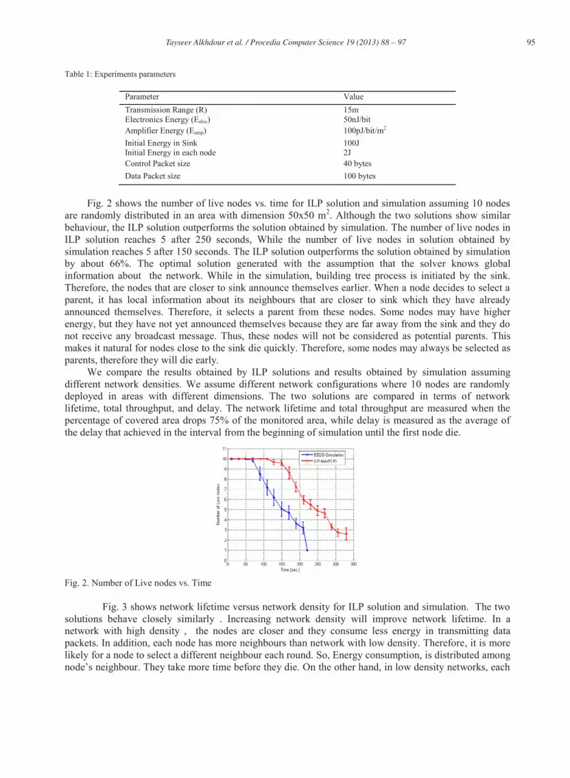
Fig. 2 shows the number of live nodes vs. time for ILP solution and simulation assuming 10 nodes

are randomly distributed in an area with dimension 50x50 m2. Although the two solutions show similar behaviour, the ILP solution outperforms the solution obtained by simulation. The number of live nodes in ILP solution reaches 5 after 250 seconds, While the number of live nodes in solution obtained by simulation reaches 5 after 150 seconds. The ILP solution outperforms the solution obtained by simulation by about 66%. The optimal solution generated with the assumption that the solver knows global information about the network. While in the simulation, building tree process is initiated by the sink. Therefore, the nodes that are closer to sink announce themselves earlier. When a node decides to select a parent, it has local information about its neighbours that are closer to sink which they have already announced themselves. Therefore, it selects a parent from these nodes. Some nodes may have higher energy, but they have not yet announced themselves because they are far away from the sink and they do not receive any broadcast message. Thus, these nodes will not be considered as potential parents. This makes it natural for nodes close to the sink die quickly. Therefore, some nodes may always be selected as parents, therefore they will die early.

We compare the results obtained by ILP solutions and results obtained by simulation assuming different network densities. We assume different network configurations where 10 nodes are randomly deployed in areas with different dimensions. The two solutions are compared in terms of network lifetime, total throughput, and delay. The network lifetime and total throughput are measured when the percentage of covered area drops 75% of the monitored area, while delay is measured as the average of the delay that achieved in the interval from the beginning of simulation until the first node die.

Fig. 2. Number of Live nodes vs. Time

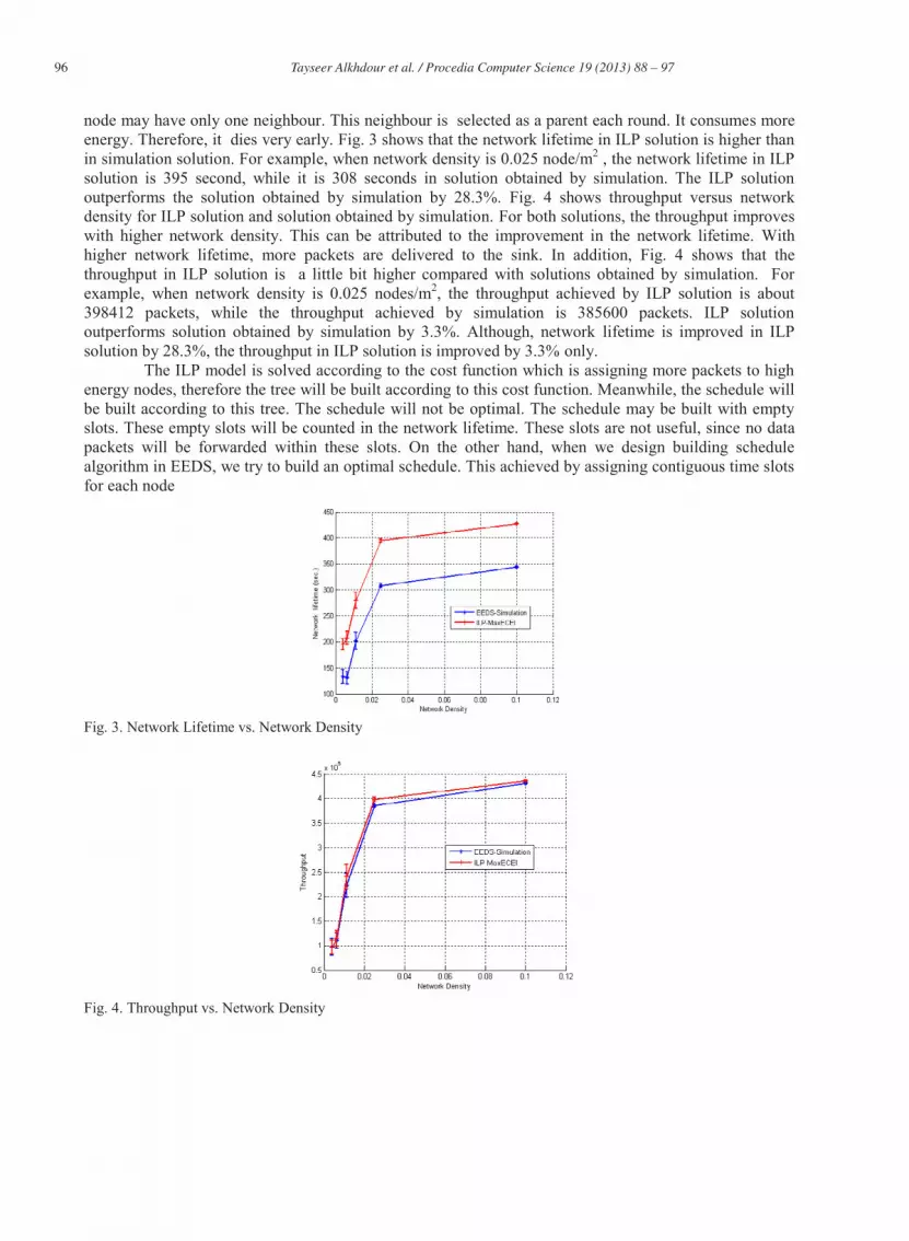
Fig. 3 shows network lifetime versus network density for ILP solution and simulation. The two solutions behave closely similarly . Increasing network density will improve network lifetime. In a network with high density , the nodes are closer and they consume less energy in transmitting data packets. In addition, each node has more neighbours than network with low density. Therefore, it is more likely for a node to select a different neighbour each round. So, Energy consumption, is distributed among

neighbour. They take more time before they die. On the other hand, in low density networks, each


node may have only one neighbour. This neighbour is selected as a parent each round. It consumes more energy. Therefore, it dies very early. Fig. 3 shows that the network lifetime in ILP solution is higher than in simulation solution. For example, when network density is 0.025 node/m2 , the network lifetime in ILP solution is 395 second, while it is 308 seconds in solution obtained by simulation. The ILP solution outperforms the solution obtained by simulation by 28.3%. Fig. 4 shows throughput versus network density for ILP solution and solution obtained by simulation. For both solutions, the throughput improves with higher network density. This can be attributed to the improvement in the network lifetime. With higher network lifetime, more packets are delivered to the sink. In addition, Fig. 4 shows that the throughput in ILP solution is a little bit higher compared with solutions obtained by simulation. For example, when network density is 0.025 nodes/m2, the throughput achieved by ILP solution is about 398412 packets, while the throughput achieved by simulation is 385600 packets. ILP solution outperforms solution obtained by simulation by 3.3%. Although, network lifetime is improved in ILP solution by 28.3%, the throughput in ILP solution is improved by 3.3% only.

The ILP model is solved according to the cost function which is assigning more packets to high energy nodes, therefore the tree will be built according to this cost function. Meanwhile, the schedule will be built according to this tree. The schedule will not be optimal. The schedule may be built with empty slots. These empty slots will be counted in the network lifetime. These slots are not useful, since no data packets will be forwarded within these slots. On the other hand, when we design building schedule algorithm in EEDS, we try to build an optimal schedule. This achieved by assigning contiguous time slots for each node

Fig. 3. Network Lifetime vs. Network Density

Fig. 4. Throughput vs. Network Density


5. Conclusion

Recently, wireless sensor networks (WSNs) have received a growing attention due to their potential in many real-life applications. This research has tackled an important issue that is jointly design routing and scheduling mechanism for periodic-data gathering in designing WSN. We have proposed a new ILP formulation for randomly deployed wireless sensor nodes. The ILP model is examined via extensive numerical examples. Moreover, the numerical results have been compared with EEDS which is a heuristic approach for constructing jointly a routing and a scheduler for WSN. In the future, we are planning to introduce additional cost functions to take into account other performance metrics, such as delay.

References

[1] I. F. Akylidiz, W. Su, Y. Sankarasubramaniam, E. Cayirci. A survey on sensor networks. IEEE Personal Communications Magazine, August 2002; 102-114.

[2] Wendi R H, Anantha P C, Hari B. An Application-Specific Protocol Architecture for Wireless Microsensor Networks. IEEE On Wireless Communications Trans., vol. 1, No. 4, Oct. 2002; 660-670.

[3] Azzedine B, Xuzhen C, Joseph L. A Performance Evaluation of a Novel Energy-Aware Data-Centric Routing Algorithm in Wireless Sensor Networks. Wireless Networks 11, 2005; 619 635.

[4] Lianshan Y, Wei P, Bin L, Xiaoyin L, Jiangtao L. Modified Energy-Efficient Protocol for Wireless Sensor Networks in the Presence of Distributed Optical Fiber Senor Link. Sensors Journal, IEEE , vol.11, no.9, pp.1815-1819, Sept. 2011.

[5] Srikanth, B, Harish M, Bhattacharjee R. An energy efficient hybrid MAC protocol for WSN containing mobile nodes. the 8th International Conference on Information, Communications and Signal Processing (ICICS) 2011. pp.1-5, 13-16 Dec. 2011

[6] Tayseer A, Uthman B. An Energy-Efficient Distributed Schedule-Based Communication Protocol for Wireless Sensor Networks. The Arabian Journal for Science and Engineering (AJSE), Vol. 35, Number 2B; October 2010, 153-168.

[7] Seung-Jun K, Xiaodong W, Madihian M. Joint Routing and Medium Access Control for Lifetime Maximization of Distributed Wireless Sensor Networks. In Proceedings of the IEEE International Conference on Communications (ICC). Istanbul, Turkey, 2006; 3467-3472.

[8] Madan R, Shuguang C, Lall S, Goldsmith, A.J. Modeling and Optimization of Transmission Schemes in Energy-Constrained Wireless Sensor Networks. IEEE/ACM Transactions on networking, Vol. 15, No. 6, December 2007; 1359-1362.

[9] Ali C, Samuel P. Energy-Efficient State Scheduling for Maximizing Sensor Network Lifetime under Coverage Constrain. In The Proceedings of the Third IEEE International Conference on Wireless and Mobile Computing, Networking and Communications, White Plains, New York, USA, 2007; 63.

[10] Katerina P, Vasilis F. Joint Routing and Gateway Selection in Wireless Mesh Networks. In Proceedings of the Wireless Communications and Networking Conference, March 31-April 3 2008; 2325-2330.

[11] Lucas D.P. M, Joel J.P.C. R. A survey on Cross-layer solutions for wireless sensor networks. Journal of Network and Computer Applications, Volume 34, Issue 2, March 2011, Pages 523 534

[12] IBM ILOG CPLEX Optimizer , http://www-01.ibm.com/software/integration/optimization/cplex-optimizer/ , accessed , January 2013,

[13] Shijin D, Lemin L, Du X. A Novel Cluster Formation Approach Based on the ILP for Wireless Sensor Networks. In Proceedings of the First International Conference on Communications and Networking (ChinaCom '06) , China, Oct. 2006; 1-5, 25-27.

[14] Ali C, Samuel P, On the Planning of Wireless Sensor Networks: Energy-Efficient Clustering under the Joint Routing and Coverage Constraint. IEEE Transactions on Mobile Computing, Vol. 8, No. 8, August 2009; 1077-1086.

[15] Lindo systems, http://www.lindo.com, accessed, January 2013.

Documents

An Optimal Cross-Layer Scheduling for Periodic WSN Applications