Interdependent binary choices under social influence: phase diagram for

homogeneous unbiased populations

Ana Fernandez del Rıo1, Elka Korutcheva2 and Javier de la Rubia

Departamento de Fısica Fundamental, Universidad Nacional de Educacion a Distancia (UNED)

Facultad de Ciencias (UNED), Paseo Senda del Rey 9, E-28040 Madrid

Number of text pages: 18 (including this one)

Number of figures: 8

Number of tables: 0

1E-mail: ana.fernandez@invi.uned.es Tel: (00 34) 913987143 Fax: (00 34) 9139866972Also at G. Nadjakov Institute of Solid State Physics, Bulgarian Academy of Sciences, 1784 Sofia (Bulgaria).

Abstract

Coupled Ising models are studied in a discrete choice theory framework, where they can be understood to represent

interdependent choice making processes for homogeneous populations under social influence. Two different coupling

schemes are considered. The nonlocal red or group interdependence model is used to study two interrelated groups

making the same binary choice. The local or individual interdependence model represents a single group where agents

make two binary choices which depend on each other. For both models, phase diagrams, and their implications in

socioeconomic contexts, are described and compared in the absence of private deterministic utilities (zero opinion

fields).

Nontechnical Abstract

Models of ferromagnetism are used to study populations of identical individuals making binary choices. Two cases

are considered. The first one is concerned with the interplay between two related groups making the same decision.

In the second one, a single group where each individual is making two interdependent choices is studied. The work

is focused in understanding and comparing the qualitative average outcome (phase) for the models depending on

the strength of social influence, dependence between both groups/choices and statistical fluctuations, for the simple

particular case where individuals have no particular inherent preferences regarding the decision.

Keywords

statistical physics of socioeconomic systems, opinion dynamics, discrete choice theory, coupled Ising models

2

1 Introduction

Social scientists have been interested in the formal study of discrete choice theory settings for decades. These allow for

the consideration of a wide variety of problems, ranging from the study of social pathologies [1] to demand contexts

blue [2, 3, 4, 5, 6, 7] or election results [8, 9], as well as the prevalence of different relevant social traits or opinions

[5, 10, 11, 12, 13, 14]. Traditionally, the effects of social influence were neglected. Some of the work by Schelling

[15, 16, 17] and Becker [18, 19] are exceptions, for some of which direct links to models from condensed matter can be

drawn blue [20, 21, 22]. Interactive setups similar to the ones that will be considered in this paper were introduced by

Follmer [23] and Granovetter [24]. In the 1990s, economists such as Blume, Brock and Durlauf started developing a

consistent framework in which to systematically study these problems taking into account social interactions and noted

the deep connections to some models from statistical physics [25, 26, 27, 28]. These ferromagnetic setups had also been

already proposed by some of the first physicist advocates of building a physics like body of knowledge for the social

sciences [10, 29, 30].

The traditional approach typically considers a group of agents maximising the utility function:

U(si, hi, Ei(~s), ǫi(si)) = u(si, hi) + S(si, Ei(~s)) + ǫi(si) (1.1)

where u is the private deterministic utility, S the social deterministic utility and ǫi the private random utility. The choice

si made by the individual i can take the values -1 or 1. Each is a component of vector ~s, with Ei(~s) representing the ith

agent’s subjective belief on the choices of the rest of the agents. The idiosyncratic willingness to adopt (hereafter IWA)

or opinion field hi characterises personal preferences of each agent, its inherent predisposition towards the choice making

process. Finally, ǫi is an individual and choice dependent random shock. Economic demand contexts can be studied in

these setups by interpreting IWAs as a combination bi − p, where bi is the idiosyncratic willingness to buy (hereafter

IWB) and p the fixed price. Demand curves, i.e., the dependence on price of the fraction of adopters µ (fraction of

the individuals with si = 1), can be studied for fixed values of the rest of the parameters, as discussed, for example, in

[2, 4, 7, 31].

There is a direct analogy that can be established between these settings (and their total utility) and condensed matter

models for ferromagnetism (and their total energy). The binary choice variable si can be understood as a binary spin

variable and so the average choice s = 1N

∑

i si as the system’s average magnetisation, which can be easily expressed in

terms of the fraction of adopters µ as s = 2µ− 1. The action of the IWA hi, and therefore of private deterministic utility

terms, will be associated in its ferromagnetic counterpart to the action of magnetic fields. Social deterministic utility can

be related to spin interactions. Random private utility is translated into the introduction of random noise. Assuming a

logistic distribution for the difference of the random payoff terms P (ǫi(−1)− ǫi(1) ≤ z) = 11+e−βz identical for all agents,

is equivalent to studying the ferromagnetic system using the canonical ensemble, i.e., in statistical equilibrium. Note that

in the physical model, β is given the statistical mechanical usual interpretation of inverse of the temperature β = 1/KBT ,

were KB is Boltzmann’s constant. In discrete choice settings, socioeconomic temperature, 1/β in the utility discrete

choice setting, represents statistical fluctuations that can reflect an incomplete knowledge about agent’s particularities,

individuals’ probability of behaving irrationally and/or a more fundamental uncertainty concerning free will. This allows

for an interpretation of β in terms of social permeability, which measures the potential response of individuals to social

influence [10].

Under particular choices for private and social deterministic utilities, the system can be described using a mean field

Ising model with constant external field [26, 27], that was solved exactly in the 1930s (see for example [32]). This is

only true when considering a private deterministic utility u proportional to both the individual’s choice and the IWA,

3

which is considered the same for all agents (constant opinion field). Social deterministic utility will have as many

terms as other agents with whom there is interaction. All agents are assumed to interact with all others and each of

these terms to be proportional to the quadratic difference between the agent’s opinion and its perception of the other’s

choice: S = −Ei

(

∑

j 6=i

Jij

2 (si − sj)2)

. The coupling Jij measures how much agent i wants to conform to the opinion

of agent j and thus the strength of social influence/magnetic interaction and is also assumed to be constant throughout

the population 3. Agents have rational expectations, i.e., Ei(sj) = s. Note this means all individuals will be equally

compelled to align their opinions with the average choice. All agents have the same (accurate) perception of what the

average behaviour of the group is. As all agents also have identical IWAs, populations are completely homogeneous.

These are drastic simplifications concerning most socioeconomic systems of interest but are useful to understand

basic qualitative features emerging from social interaction. Complexity can be added and hypothesis relaxed to make

them more realistic and parallelisms to statistical physics still remain useful. It seems particularly relevant to include

heterogeneity that enables the characterisation of the group. This can be achieved using random fields and/or spin glass

type models, which have been extensively studied in physics [33, 34, 35, 36, 37, 38]. Work on these lines in socioeconomic

contexts can be found in [4, 5, 7, 14, 26, 28, 30, 31, 39, 40]. Other interesting variations on the interacting scheme, such

as nearest neighbours or similar [1, 3, 5, 8, 9, 13, 23, 26, 28, 41, 42, 43], dynamic interacting neighbourhoods [40, 44] or

complex networks [8, 43, 45] can be used. However, the mean field approach can be argued to be a good approximation

for many problems of interest to mimic a general tendency to conform to the norm and is more tractable analytically

[4, 7, 10, 12, 14, 26, 27, 28, 30, 31, 39, 40, 46, 47]. Relaxing rational expectations and/or reciprocity assumptions [1, 31, 46]

are also interesting paths to explore, as is the study of finite size effects [30, 39, 40]. The study of this kind of setups as

dynamical systems (which can evolve out of equilibrium) [3, 8, 9, 11, 12, 13, 31, 41, 42, 44, 45] is currently an active area

of research sometimes referred to as opinion dynamics (see [40] and [48] for reviews). Similar setups can also be used to

study other related problems such as resource allocation, hierarchical structures, coalition formation, social learning, and

public goods games [2, 6, 20, 23, 25, 40, 43, 46, 47, 48, 49].

When comparing discrete choice settings subject to social influence to those without, interesting qualitatively different

characteristics appear. Even the simple Ising mean field model with constant field already presents a rich statistical

mechanical phenomenology [32] with interesting translations to socioeconomic language [10, 12, 26, 27, 28, 30, 39]. The

qualitative average outcome (phase) is described by its order parameter, the average choice s. For the unpolarised or

paramagnetic phase (s = 0), in average half of the group is deciding for and half against. In the polarised or ferromagnetic

state (s 6= 0), there is a greater prevalence of one of the options over the other.

Unbiased populations (with respect to a particular choice) are those with zero IWA for all individuals. The average

outcome will be determined only by social interaction, individuals having no inherent deterministic preference for any

of the choices. We can for example consider this to be the case for some fashions and traditions, where there is no real

cost or benefit for the individuals besides the social payoff provided through imitation. The unpolarised state can only

be stable in this case, with a second order phase transition for Jβ = 1, where a system will experience a rapid but

continuous change from an unpolarised state (for low social permeability β or high social coupling J) to a polarised one.

In the polarised regime (1 < Jβ), the stable equilibrium is degenerate, as there are two identical maxima of the utility

s = ±m (minima of the free energy, physically equivalent states). The previous history of the system becomes relevant

and microeconomic specifications of the model may not uniquely determine its macroeconomic properties.

When we turn on the opinion fields, these critical values of the parameters for which a second order phase transition

3Dimensionless choice variables si are considered, and so utility, social coupling, IWA and temperature are measured in the same units

(formally equivalent to the physical scenario in natural units ~ = KB = 1), which can be defined to suit the specific problem under consideration.

They can be an attempt to quantify abstract quantities (satisfaction, wellbeing, reputation. . . ) or measure specific gains or losses (surpluses

or deficits) of the individuals, for example, in money.

4

takes place for the unbiased case, still separate regions where social utility is relevant (spontaneous magnetisation exists

in the physical analog) and regions where it is not. Systems in a previously unpolarised state at h = 0 will turn into

well behaved, single stable polarised states, with the sign of the average choice determined by that of the population’s

IWA. If the system was already in a polarised state at zero IWA, while the sign and value of the average choice will

in general be unambiguously determined by that of the field, for small enough values of the latter, the symmetry is

not completely broken and the degeneracy of the average choice equilibria persists. While no longer equiprobable or

symmetric, depending on the previous state of equilibrium of the system, the final average magnetisation may not be

aligned with the IWA. Metastable states can be understood as a collectively reinforced choice that persists even when

the rest of conditions are ripe for a change in the sign of the average choice. In economic demand contexts, it involves

two coexisting low and high demand states for a given price. They are associated to a first order phase transition at

h = 0, which provides a mechanism for abrupt, discontinuous changes in the sign of the average choice and the possibility

for hysteresis (changes in the state of the system when varying the parameters that can not be undone by reversing the

process).

Some attempts at explaining data referring to real social processes using this type of approach have been made

[1, 2, 5, 8, 9, 11, 14]. This line of research remains, however, somewhat scarce, and more efforts need to be put in this

direction.

In this work, besides considering social influence, two different binary choice variables, each governed by Ising mean

field dynamics, are coupled in another ferromagnetic like interaction. These and similar setups have been studied in

physical contexts, particularly for their interest in explaining plastic phase transitions [50, 51, 52, 53, 54, 55]. It amounts

to the introduction of an additional contribution to the utility (1.1) that bonuses or penalises agents for the alignment

of both spin variables. This is the case of interest when considering two different groups making the same choice when

both groups are interdependent in their decision making process. Each individual is subject to social pressure to conform

to its own group’s average. Besides, agents will also tend to align (k > 0) or dis-align (k < 0) their options with the

other group’s average choice. This setup is referred to as the group interdependence or the nonlocal model (agents can

be considered to interact with all members from its own group and the other one). Coupled spin variables are also the

case of interest to study a single group in which each individual has to make two choices which are related, which can be

labelled individual interdependence or local model (the coupling between both spin variables is then only through each

individual). These systems can be in three possible phases depending on the two (coupled) order parameters: unpolarised

or paramagnetic phase (s = t = 0), polarised or ferromagnetic phases (s 6= 0, t 6= 0) and mixed phases (one zero and one

nonzero order parameter)4.

In the next two sections, Hamiltonians for both models are described and expressions for their free energies and

systems of equations of state analytically derived. Section 4 describes and compares the resulting phase diagrams for the

zero opinion fields or unbiased case. Finally, some concluding remarks are made.

2 The group interdependence or nonlocal model

Let us consider two groups, one made up of Ns agents making binary choice si = ±1 and the other of Nt agents making

binary choice ti = ±1 with dynamics governed by the Hamiltonian:

H =∑

(i,j)

(

−JsNs

sisj −JtNt

titj −k(Ns +Nt)

2NsNt

sitj

)

−∑

i

(hssi + htti) (2.1)

4This terminology convention is different from that used in [55], where the ferromagnetic phase is referred to as mixed phase.

5

where summations over (i, j) are 1 ≤ i < j ≤ Ns for the first term, 1 ≤ i < j ≤ Nt for the second term and 1 ≤ i ≤ Ns,

1 ≤ j ≤ Nt for the mixed term. Summations over i are 1 ≤ i ≤ Ns for the fourth term and 1 ≤ i ≤ Nt for the last term.

The intra-couplings Js, Jt are positive and constant and quantify the strength of social pressure within each group.

Each individual’s decision is also affected by the agent’s correct perception of what the other group is doing through

the inter-coupling k. It may either reinforce (k > 0) or discourage (k < 0) alignment of choices between individuals in

different groups but interaction is always symmetric (exactly reciprocal). Using mean field theory, which is exact for

infinite groups (thermodynamic limit in physical terminology), is equivalent to considering each agent as influenced by its

correct perception of the average choice of the other group. Besides intra- and inter- group social interactions, each group

is subject to a constant opinion field. The most natural application seems to problems where the interaction between both

groups is of social nature. It could also refer, however, to actual gains or losses for agents unrelated to social interaction.

This setup could be used to study problems such as the incidence of social pathologies in neighbouring districts,

public opinion on a certain issue in two neighbouring countries, technology choice in two different related industries,

female participation in the labour market in two neighbouring regions, etc.

When both groups are of the same size (which is the case when considering infinitely large groups) this is the system

studied in [52]. This work extends the results presented there using numerical methods to calculate stable solutions of

the system in thermodynamic equilibrium.

For Ns = Nt = N , using mean field theory (on all intra- or inter-coupling terms) we can rewrite (2.1) as:

H =NJs2

s2 +NJt2

t2 +Nkst− (Jss+ kt+ hs)∑

i

si − (Jtt+ ks+ ht)∑

i

ti (2.2)

where s = 1N

∑

i si and t = 1N

∑

i ti are the average choices in each of the groups. The corresponding partition function

for the representative canonical ensemble (Z = Tre−βH where Tr indicates sum over all possible spin configurations) can

be expressed

Z = e−β(N2s2Js+

N2t2Jt+Nkst)[2 cosh (β (Jss+ kt+ hs)) 2 cosh (β (Jtt+ ks+ ht))]

N (2.3)

where β is the social permeability or inverse of the temperature (which in this case accounts for statistical fluctuations).

Finally the system’s free energy density (f = F/N with F the free energy F = β−1 log(Z)) will be given in the mean

field approximation by

f =1

2Jss

2 +1

2Jtt

2 + kst−1

βln (2 cosh (β (Jss+ kt+ hs)))−

1

βln (2 cosh (β (Jtt+ ks+ ht))) (2.4)

Stable states of the system will be those minimising the free energy. After derivation and simple algebraic manipulation,

critical points can be found to be given by the system of equations of state:

a (s− tanh (β (Jss+ kt+ hs))) = 0

a (t− tanh (β (Jtt+ ks+ ht))) = 0(2.5)

with a = JsJt − k2.

There are thus two different cases. For the degenerate case (a = 0), substituting Jt = Js/k2 in the original system

both give the same equation of state:

Jss+ kt− Js tanh (β (Jss+ kt+ hs))− k tanh

(

β

(

k2

Jst+ ks+ ht

))

= 0 (2.6)

For the non-degenerate case (a 6= 0), on which this work focuses, critical points will be given by solutions to the

system of equations of state:

6

s = tanh[β (Jss+ kt+ hs)]

t = tanh[β (Jtt+ ks+ ht)](2.7)

Positive definite Hessian (evaluated at the solution of the system (2.7)) is a sufficient condition for a critical point to

be a minimum. In this case, its determinant can be written as:

det(H) = a (1− βJsγs − βJtγt) + β2a2γsγt (2.8)

and the free energy’s second derivative (and first diagonal element of the Hessian) as:

∂2f

∂s2= Js − βJs

2γs − βk2γt (2.9)

where γs =1

cosh2[β(Jss+kt+hs)]and γt =

1cosh2[β(Jtt+ks+ht)]

. Positive (2.8) and (2.9) are sufficient conditions for minima.

When zero opinion fields are considered, polarised solutions of the system of equations of state (2.7) will always

appear in pairs (s, t) and (−s,−t), each pair of solutions having the same stability. There is also a symmetry relating

solutions under a change in sign in k and in any one of the average magnetisations. Furthermore, the unpolarised state or

paramagnetic solution s = t = 0 is always a critical point of f . Critical regions where its stability changes can be studied

by linearising equations (2.7) for |s| ≪ 1 and |t| ≪ 1 (at finite non zero temperature) when hs = ht = 0, yielding:

s = β (Jss+ kt) +O(s3, t3, s2t, st2)

t = β (Jtt+ ks) +O(s3, t3, s2t, st2)(2.10)

.

Further simplification of this system leads to the expression:

aβ2 − (Js + Jt)β + 1 = 0 (2.11)

.

Solving (2.11) gives two values of β where the stability of the paramagnetic phase changes from saddle point to

maximum/minimum:

β =Js + Jt ±

√

(Js + Jt)2 − 4a

2a=

Js + Jt ±√

(Js − Jt)2 + 4k2

2a(2.12)

In the strong coupling regime (k2 > JsJt), there is a single physical (positive) value, where the unpolarised solution

changes from saddle point to maximum, and so of no relevance in the discussion of phase transitions.

In the weak coupling regime (k2 < JsJt), there will be two physical values of β. The larger one (given by the + option

in (2.12)) is of the same type as discussed above. The smaller one (given by the −), is a critical point at which the

unpolarised or paramagnetic phase will change from saddle to minimum and a second order phase transition takes place.

For temperatures bellow the critical one, the system is in a polarised or ferromagnetic phase. This means that, even in

the absence of personal predispositions of any type, social interaction both with individuals from within the agent’s own

group and from the other one, promotes the emergence of a tendency to polarisation (which is only complete, i.e., s = ±1

and t = ±1 at T = 0). The actual direction of choice is not determined, only the alignment or dis-alignment between

both average choices (there are two physically equivalent states of equilibrium). Note that when opinion fields are turned

on, even if the symmetry is broken and the paramagnetic solution will no longer be a critical point, this will still delimit

regions of the phase diagram where interaction in itself has an impact on the aggregate outcome.

7

3 The individual interdependence or local model

Let us now consider a single group of N identical individuals all of which are simultaneously making two interdependent

binary choices si = ±1 and ti = ±1. There will be an additional term in the utility function that penalises or bonuses

the agent for aligning or not its two choices. Both of the decisions are subject to social influence to conform to the norm

and to a constant opinion field. A Hamiltonian describing such a system is:

H =∑

(i,j)

(

−JsN

sisj −JtN

titj

)

−∑

i

(ksiti + hssi + htti) (3.1)

where summations over (i, j) are 1 ≤ i < j ≤ N and summations over i are 1 ≤ i ≤ N . Note that in this case the

interaction between both choice variables cannot be of social nature.

Discrete choice problems of interest to the social sciences that can be explored using this model include the relation

between teenage pregnancy and school dropout in a given population, results in simultaneous referendums or in elections in

a bipartidist system, demand for two different software products of the same brand, motherhood and female participation

in the labour market and so on.

This is a similar model to that studied in [55], where random inter-coupling k is considered. Most results presented,

however, are for symmetric probability distributions p(ki) which seem of little interest in the socioeconomic context, as

they involve populations for which half of its members have a positive interaction between both choices while for the

other half they tend to oppose.

Hamiltonian (3.1) can be rewritten:

H =Js + Jt

2−

Js2N

(

∑

i

si

)2

−Jt2N

(

∑

i

ti

)2

−∑

i

(ksiti + hssi + htti) (3.2)

Following [55], the partition function of the representative canonical ensemble can be computed exactly for an infinitely

large system (thermodynamic limit) yielding:

Z =βN

2π(JsJt)

1

2 e−β2(Js+Jt)

∫ ∞

−∞

∫ ∞

−∞

ds dte−βNg(s,t) (3.3)

where g(s, t) is the free energy functional such that the free energy density f = limN→∞FN

=∫∞

−∞

∫∞

−∞ ds dt g(s, t) and

is given by the expression:

g =1

2Jss

2 +1

2Jtt

2 −1

βln[2eβk cosh (β (Jss+ Jtt+ hs + ht)) + 2e−βk cosh (β (Jss− Jtt+ hs − ht))] (3.4)

Critical points of the free energy f are those of the functional g. Introducing the notation αs = tanh (β(Jss+ hs)),

αt = tanh (β(Jtt+ ht)) and αk = tanh (βk), the system’s equations of state can be written as:

s =αs + αtαk

1 + αsαtαk

t =αt + αsαk

1 + αsαtαk

(3.5)

In this case the Hessian’s determinant takes the form:

det(H) = JsJt[1−β(

Jtγt(1− α2sα

2k) + Jsγs(1− α2

tα2k))

(1 + αsαtαk)2+

β2JsJtγsγt(

(1− α2sα

2k)(1 − α2

tα2k)− γsγtα

2k

)

(1 + αsαtαk)4] (3.6)

8

and g’s second derivative with respect to s is given by:

∂2g

∂s2= Js −

βJ2s γs

(

1− α2tα

2k

)

(1 + αsαtαk)2(3.7)

The zero opinion field case has the same symmetries described for the nonlocal non-degenerate zero field model. The

paramagnetic or unpolarised solution is also always a critical point of g. Linearization of (3.5) for |s| ≪ 1 and |t| ≪ 1 (at

finite nonzero temperature) when hs = ht = 0 yields:

s = βJss+ βJt tanh(βk)t+O(s3, t3, s2t, st2)

t = βJtt+ βJs tanh(βk)s+O(s3, t3, s2t, st2)(3.8)

which can be simplified to

JsJt(

1− tanh2(βk))

β2 − (Jt + Js)β + 1 = 0 (3.9)

Depending on the values for the intra- and inter-couplings, there can be three qualitatively different scenarios when

analysing equation (3.9), with either one, two or three different solutions in β (all positive and thus physically relevant). In

all cases, only the smaller (or only) one of these (the highest temperature) will be a critical point where the paramagnetic

or unpolarised phase becomes unstable and there is a second order phase transition taking place.

4 Phase diagrams for the unbiased case

The Newton−Raphson algorithm has been used to numerically solve the equations of state for the unbiased case (hs =

ht = 0), fixed Js = 1 in some given units (which is equivalent to measuring the rest of couplings and fields in terms of

Js) and different values of the rest of the parameters. Python libraries developed for the computation and analysis of

these are available at https://github.com/anafrio/. Results are summarised through figures of the phase diagram’s

cross-sections for both models for specific values of the rest of parameters. These have been chosen for the sections to

be representative of all the possible phenomenology. More details on the solutions found (including unstable ones) and

dependence on the different parameters can be found in [56].

Unbiased situations refer to what has been loosely referred to as trends or traditions, i.e., social conventions which

will give no particular advantage or disadvantage to the isolated individual and choice. For the group interdependence

model, this would be the case, for example, to study the use of a particular outfit or accessory in two different socioe-

conomic groups, or the adoption of specific vocabulary (argot, technical term) by two such groups. Unbiased individual

interdependence could be of use to tackle problems such as how the use of an accessory in a group will be affected by the

use of another when it is considered to be fashionable or unfashionable to wear them together.

The study of the unbiased case is also useful to get some insight on what will happen in a more general situation

of biased homogeneous groups. The introduction of nonzero constant opinion fields, will in general determine the sign

of the average magnetisation and break the equilibria degeneracy, and the unpolarised state will no longer be stable.

What were unpolarised regions for the unbiased case, will become characterised by an equilibrium demand or acceptance

univocally determined by the constant IWA (or IWB and price). In the already polarised regions before the introduction

of fields, however, multiple possible equilibria and first order phase transitions can be expected at low enough IWAs and

temperatures [57].

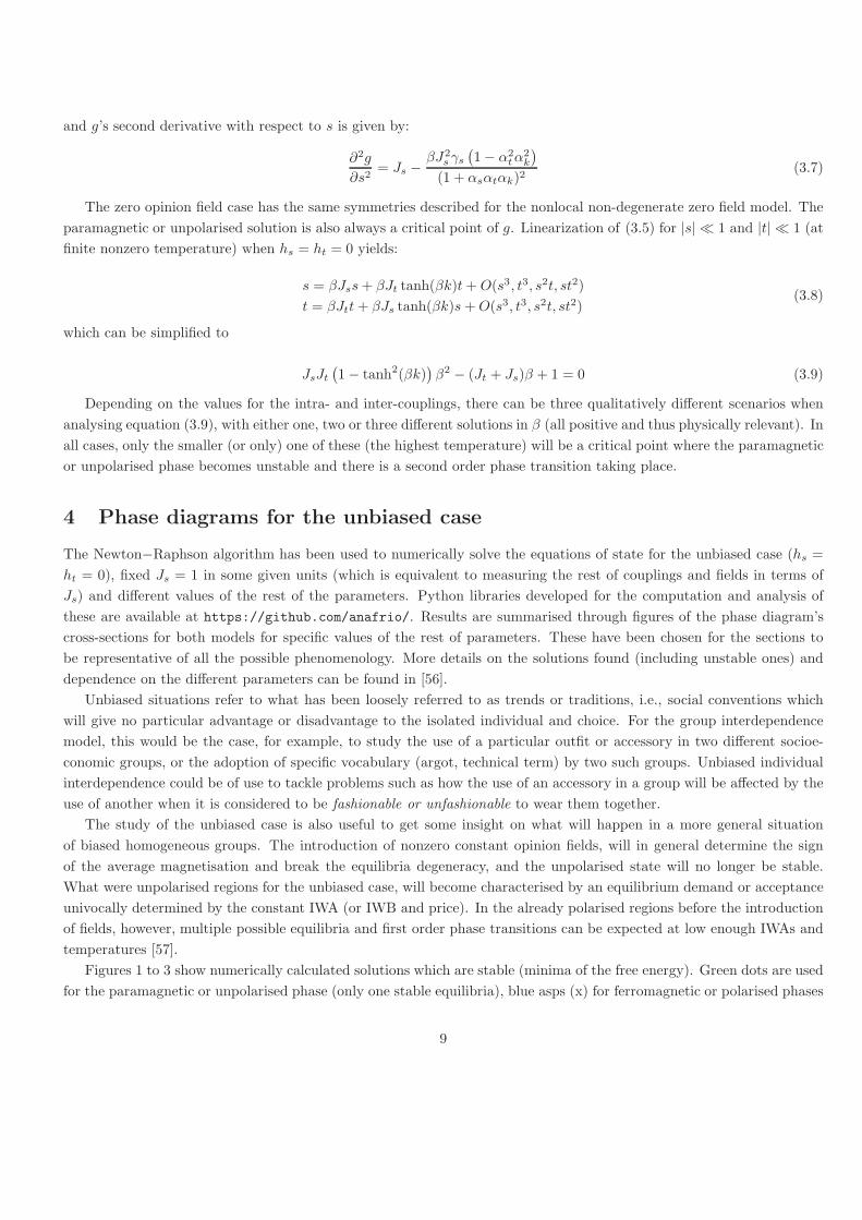
Figures 1 to 3 show numerically calculated solutions which are stable (minima of the free energy). Green dots are used

for the paramagnetic or unpolarised phase (only one stable equilibria), blue asps (x) for ferromagnetic or polarised phases

9

with both average choices of the same sign and crosses (+) for ferromagnetic or polarised phases with average choices of

opposed signs (two physically equivalent stable equilibria in each case). Red triangles show mixed phase solutions (also

two equilibria). When both types of ferromagnetic or polarised phases are superposed, there are four different equilibria,

two stable (those aligned according to the sign of k) and two metastable.

The mixed segment is shown with a dashed black line (figures 2 and 3). This is the only region where mixed phases

are solutions and is the same for both models as these can only exist for k = 0 (uncoupled case) and when one of the

Ising models is in the paramagnetic phase while the other is still in the ferromagnetic phase, i.e., Jt < β−1 < Js when

Jt < Js (or Js < β−1 < Jt when Js < Jt). Whenever there is a nonzero value of k, it is no longer possible for the opinion

to remain unpolarised if the other group/opinion to which it is coupled is not.

For the group interdependence or nonlocal model, the degenerate curve k2 = JsJt is drawn as a solid thick black line

(figures 1 (a), 2 (a) and 3 (a) and (c)). As shown in the figures, there are no stable solutions of any type in the strong

coupling regime. Frustration prevents the system from arriving at equilibrium. This was already being indicated by

the fact that neither the completely polarised (s = ±1, t = ±1) solutions at zero temperature or the unpolarised one at

very large temperatures are stable (which can be checked analytically). When considering that the interaction between

both groups is of pure social type, assuming stronger social pressure from within the group than from the outside seems

pretty natural. It can be considered a nice feature of the model that it breaks down when the problem is, sociologically

speaking, ill defined (groups have not been chosen appropriately). The coupling between both groups, however, needs

not to be of social nature. In this case, this would be pointing at a real impossibility of arriving at a stable equilibria if

the interdependence between both groups is the main driver of the choice making process.

The critical curve, where a second order phase transition takes place, is drawn in thin solid black (figures 1, 2 and 3

(a) and (b)). This is given by the condition β−1 > max{Js, Jt} together with (2.12) for the nonlocal model or (3.9) for the

local model. It separates regions of polarised opinion (ferromagnetic phases) from others where the paramagnetic phase

is the only stable equilibria (half of the population deciding each way for both choices for sufficiently large statistical

fluctuations). When nonzero, constant IWAs are introduced, this will still separate regions where there will be a single

possible value for the average choice from those where metastable equilibria can be expected to appear for low fields.

Under such circumstances, drastic and irreversible shifts in the average opinion can be expected [57].

Figure 1 shows a Jt − β−1 section for the nonlocal (a) and local (b) models for Js = 1 and k = 0.3. They are

remarkably similar qualitatively and quantitatively. If both groups/choices were not coupled, the critical curve would be

the line of slope one across the origin and in all of the ferromagnetic region there would be two possible values (of same

absolute value) for each average magnetisation (four possible states when combined), all with the same probability. The

introduction of interdependence between both groups/choices promotes polarisation, making larger statistical fluctuations

(temperature) needed as compared to the uncoupled case for imitation to promote a certain collective trend. For high

enough social permeabilities β, there will no longer be a threshold value of the social influence bellow which the system

is in a paramagnetic phase. In the individual dependence case, even when we consider no imitation whatsoever for one of

the choices (Jt = 0), social pressure on the other is enough for polarisation to appear. This is not the case of the group

dependence model, where zero intra-couplings are forbidden, as they always lay in the strong coupling regime.

When considering ferromagnetic regions, the introduction of the coupling will, in general, fix the relative signs between

both choices, although not the direction. For example, if we consider the adoption of a certain technical term by two

professional groups or academic disciplines, if these are close and there is affinity between them, the new term will either

gain acceptance or not in both groups. Similarly, if both groups perceive each other as confronted in any way, a high

acceptance in one of them will always come with a low acceptance in the other. Likewise, if we analyse teenage outfit, if

two accessories are perceived as fitting well, they will either both be used by over half of the population or by less than

10

0.0 0.5 1.0 1.5 2.0 2.5KBT

0.0

0.5

1.0

1.5

2.0

2.5

Jt

Jt�KBT section

ferro -paraferro +

(a)

0.0 0.5 1.0 1.5 2.0KBT

0.0

0.5

1.0

1.5

2.0

Jt

Jt�KBT section

ferro -paraferro +

(b)

Figure 1: Jt − β−1 section for the (a) nonlocal and (b) local models for fixed Js = 1 and k = 0.3.

half of it, with no possibility of one of the trends being successful without the other.

For low enough temperatures and/or strong enough social pressure (coupling Jt), there is a region of metastability

and the possibility of hysteresis. This behaviour is related to a first order phase transition at k = 0. If the inter-coupling

is slowly reversing its sign, the system may not immediately change in the alignment of average choices, i.e., the system

may get trapped in a local minima of the free energy (for a while, statistical fluctuations will make the system decay to the

real ground state eventually). This is never the case for uncoupled groups/choices in the unbiased case and can be given

interesting interpretations when considering two groups/choices with mutual influence slowly changing from negative to

positive (or positive to negative). In the example of vocabulary adoption, this will imply the possibility of the use of the

word remaining low in one of the professional sectors even as the mutual perception becomes positive, before there is an

abrupt change and becomes widely accepted or not in both groups. In this region, the introduction of weak nonzero fields

will probably enrich the metastability landscape [57].

Note that for the nonlocal model the metastability region extends up to β−1 = 0 but it does not in the local case (which

can be easily checked analytically). This difference can also be explained naturally in the light of social applications. Zero

temperature is equivalent to a completely deterministic picture. Then, in the local case, each rational, utility maximiser

knows exactly whether it is better off aligning or not both of its choices (although not in which direction). In the nonlocal

case, however, although there is still a globally preferred condition of alignment or not between both groups, the choice

is not up to every agent as the coupling depends on what the other group is doing.

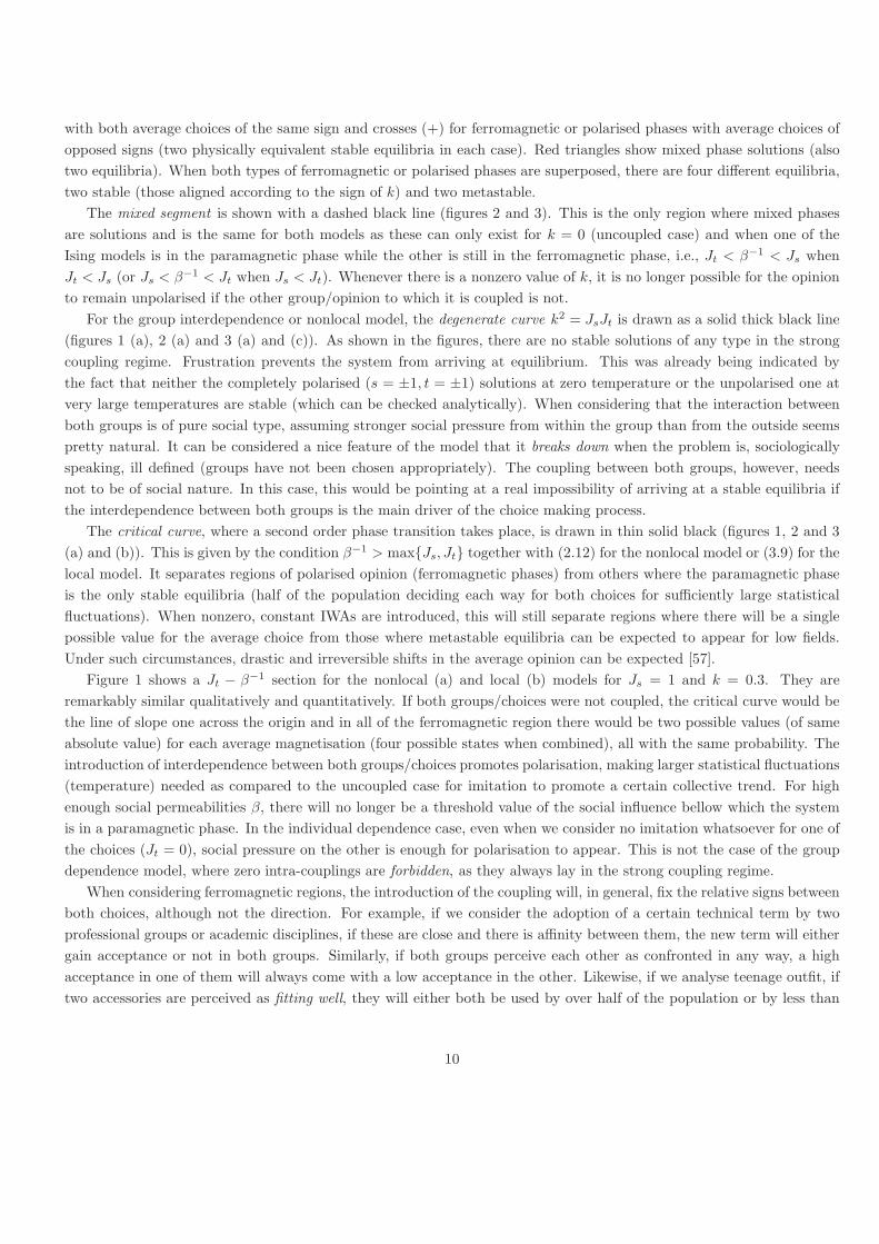
Figure 2 shows k − β−1 sections for both models when Js = 1 and Jt = 0.6. The uncoupled case is described by the

k = 0 axis. Besides the promotion of polarisation and the differences already noted when examining the Jt −β−1 section,

for the local model, the critical curve is such that lim|k|→∞ β−1 = Js + Jt = 1.6. No similar asymptotic behaviour is

shown by the nonlocal critical curve (for which high values of |k| are of little interest as there are no stable solutions

in the strong coupling regime). When the interrelation between both decisions is much more important than any of the

imitation strengths, the critical value of social permeability at which a different qualitative picture can emerge due to

social interaction, is basically determined by the intra-couplings. Further increasing |k| will have little impact in the

11

0.0 0.2 0.4 0.6 0.8 1.0 1.2 1.4 1.6 1.8KBT

�1.0

�0.5

0.0

0.5

1.0

k

k�KBT section

ferro -paraferro +mix s

(a)

0.0 0.2 0.4 0.6 0.8 1.0 1.2 1.4 1.6 1.8KBT

�1.5

�1.0

�0.5

0.0

0.5

1.0

1.5

k

k�KBT section

ferro -paraferro +mix s

(b)

Figure 2: k − β−1 section for the (a) nonlocal and (b) local models for fixed Js = 1 and Jt = 0.6.

critical value of the temperature and, once permeability is fixed and while in a high |k| range, small variations in the

interdependence of both choices will never bring about a qualitative change in the average outcome.

For both models, if β−1 > Js + Jt, the only stable state, if any, is the unpolarised one. In the nonlocal or group

interdependence model, this is due to the intersection of the degenerate curve and the critical curve, precisely at Js+Jt. In

the local or individual interdependence model, it has to do with the asymptotic behaviour of the critical curve described

above. This also makes sense in our context: at low enough permeabilities, in the local model, the interdependence

between both choices can be made as large as desired without making social influence relevant qualitatively. This means

that once we consider constant, nonzero IWAs, if the statistical fluctuations considered are large enough (such that

β−1 > Js + Jt), both average choices will be aligned with the fields, no matter what the value of k is, and no multiple

equilibria or abrupt changes will be possible.

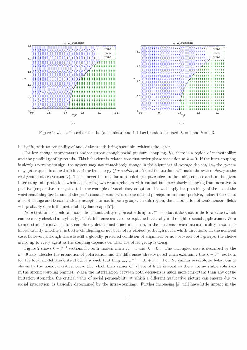
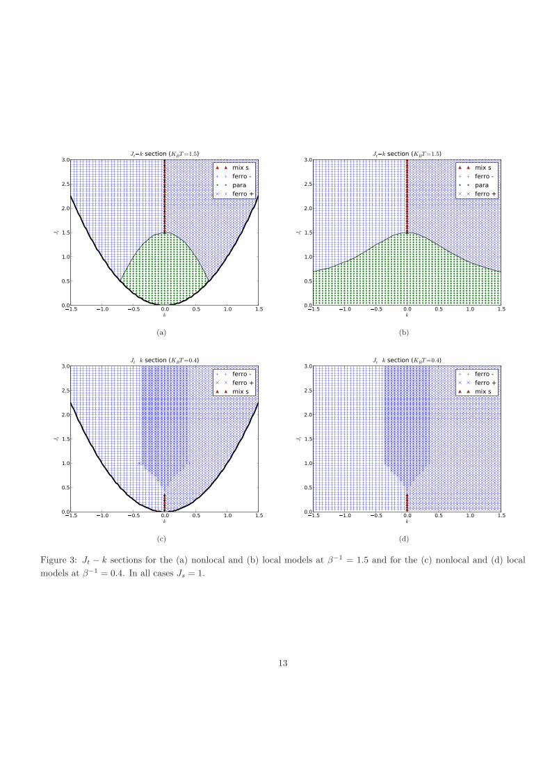
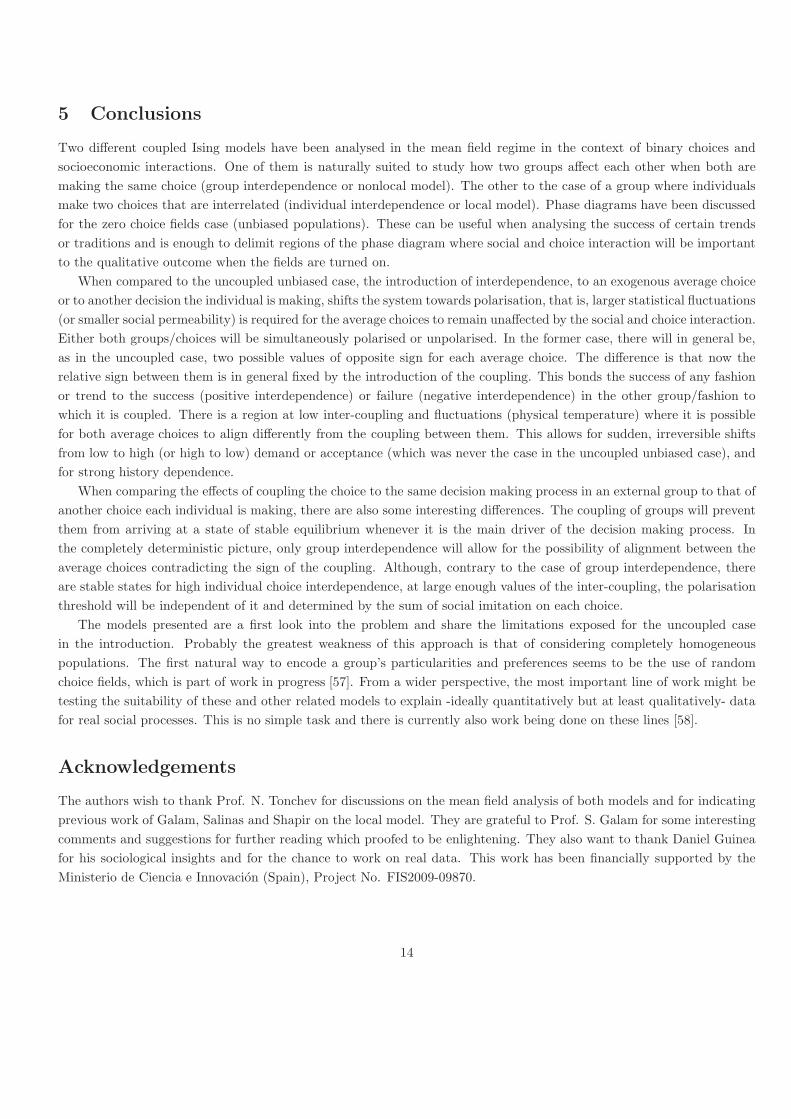
As for Jt − k sections, the situation is qualitatively different depending on the temperature chosen. Figures 3 (a) and

(b) show the sections for the nonlocal and local models when β−1 = 1.5 > Js = 1. In this case we have mixed segments

for k = 0 and Jt > β−1 = 1.5, paramagnetic phase (unpolarised collective opinions) bellow the critical curve and no

metastability region. As before, the uncoupled case is described by the k = 0 axis. Again, only the local case presents

asymptotic behaviour of its critical curve lim|k|→∞ Jt → β−1−Js = 0.4. As there, for Jt < β−1−Js, only the unpolarised

state will be stable (if any) for both models. If the dependence between both choices k is strong enough, the critical value

of Jt will be practically independent of its value.

Figures 3 (c) and (d) show the sections for the nonlocal and local models when β−1 = 0.4 < Js = 1. Mixed segments

lie, for k = 0 (uncoupled case), on 0 < Jt < β−1 = 0.4. There is no paramagnetic region (both opinions will always

be polarised). There is a region of metastability present for low enough |k| and/or high enough Jt, with the same

socioeconomic implications described above.

12

�1.5 �1.0 �0.5 0.0 0.5 1.0 1.5k

0.0

0.5

1.0

1.5

2.0

2.5

3.0

Jt

Jt�k section (KBT=1.5)

mix sferro -paraferro +

(a)

�1.5 �1.0 �0.5 0.0 0.5 1.0 1.5k

0.0

0.5

1.0

1.5

2.0

2.5

3.0

Jt

Jtk section (KBT=1.5)

mix sferro -paraferro +

(b)

1.5 1.0 0.5 0.0 0.5 1.0 1.5k

0.0

0.5

1.0

1.5

2.0

2.5

3.0

Jt

Jt�k section (KBT=0.4)

ferro -ferro +mix s

(c)

�1.5 �1.0 �0.5 0.0 0.5 1.0 1.5k

0.0

0.5

1.0

1.5

2.0

2.5

3.0

Jt

Jt k section (KBT=0.4)

ferro -ferro +mix s

(d)

Figure 3: Jt − k sections for the (a) nonlocal and (b) local models at β−1 = 1.5 and for the (c) nonlocal and (d) local

models at β−1 = 0.4. In all cases Js = 1.

13

5 Conclusions

Two different coupled Ising models have been analysed in the mean field regime in the context of binary choices and

socioeconomic interactions. One of them is naturally suited to study how two groups affect each other when both are

making the same choice (group interdependence or nonlocal model). The other to the case of a group where individuals

make two choices that are interrelated (individual interdependence or local model). Phase diagrams have been discussed

for the zero choice fields case (unbiased populations). These can be useful when analysing the success of certain trends

or traditions and is enough to delimit regions of the phase diagram where social and choice interaction will be important

to the qualitative outcome when the fields are turned on.

When compared to the uncoupled unbiased case, the introduction of interdependence, to an exogenous average choice

or to another decision the individual is making, shifts the system towards polarisation, that is, larger statistical fluctuations

(or smaller social permeability) is required for the average choices to remain unaffected by the social and choice interaction.

Either both groups/choices will be simultaneously polarised or unpolarised. In the former case, there will in general be,

as in the uncoupled case, two possible values of opposite sign for each average choice. The difference is that now the

relative sign between them is in general fixed by the introduction of the coupling. This bonds the success of any fashion

or trend to the success (positive interdependence) or failure (negative interdependence) in the other group/fashion to

which it is coupled. There is a region at low inter-coupling and fluctuations (physical temperature) where it is possible

for both average choices to align differently from the coupling between them. This allows for sudden, irreversible shifts

from low to high (or high to low) demand or acceptance (which was never the case in the uncoupled unbiased case), and

for strong history dependence.

When comparing the effects of coupling the choice to the same decision making process in an external group to that of

another choice each individual is making, there are also some interesting differences. The coupling of groups will prevent

them from arriving at a state of stable equilibrium whenever it is the main driver of the decision making process. In

the completely deterministic picture, only group interdependence will allow for the possibility of alignment between the

average choices contradicting the sign of the coupling. Although, contrary to the case of group interdependence, there

are stable states for high individual choice interdependence, at large enough values of the inter-coupling, the polarisation

threshold will be independent of it and determined by the sum of social imitation on each choice.

The models presented are a first look into the problem and share the limitations exposed for the uncoupled case

in the introduction. Probably the greatest weakness of this approach is that of considering completely homogeneous

populations. The first natural way to encode a group’s particularities and preferences seems to be the use of random

choice fields, which is part of work in progress [57]. From a wider perspective, the most important line of work might be

testing the suitability of these and other related models to explain -ideally quantitatively but at least qualitatively- data

for real social processes. This is no simple task and there is currently also work being done on these lines [58].

Acknowledgements

The authors wish to thank Prof. N. Tonchev for discussions on the mean field analysis of both models and for indicating

previous work of Galam, Salinas and Shapir on the local model. They are grateful to Prof. S. Galam for some interesting

comments and suggestions for further reading which proofed to be enlightening. They also want to thank Daniel Guinea

for his sociological insights and for the chance to work on real data. This work has been financially supported by the

Ministerio de Ciencia e Innovacion (Spain), Project No. FIS2009-09870.

14

References

[1] E. L. Glaeser, B. Sacerdote, and J. A. Scheinkman. Crime and social interactions. Quaterly Journal of Economics,

111(2):507–548, 1996.

[2] G. Weisbuch, A. Kirman, and D. Herreiner. Market organisation and trading relationships. The Economic Journal,

110:411–462, 2000.

[3] G. Weisbuch and D. Stauffer. Adjustment and social choice. Physica A, 323:651–662, 2003.

[4] M. B. Gordon, J.-P. Nadal, D. Phan, and J. Vannimenus. Seller’s dilemma due to social interactions between

customers. Physica A - Statistical Mechanics and Applications, 356(2-4):628–640, 2005.

[5] Q. Michard and J.-P. Bouchaud. Theory of collective opinion shifts: from smooth trends to abrupt swings. The

European Physical Journal B - Condensed Matter and Complex Systems, 47:151–159, 2005. 10.1140/epjb/e2005-

00307-0.

[6] A. De Martino and M. Marsili. Statistical mechanics of socio-economic systems with heterogeneous agents. Journal

of Physics A: Mathematical and General, 39(43):R465–R540, 2006.

[7] M. B. Gordon, J-P. Nadal, D. Phan, and V. Semeshenko. Discrete choices under social influence: Generic properties.

Mathematical Models and Methods in Applied Sciences, 19(1):1441–1481, 2008.

[8] A. T. Bernardes, D. Stauffer, and J. Kertesz. Election results and the sznajd model on barabasi network. European

Physical Journal B, 25(1):123–127, 2002.

[9] S. Fortunato and C. Castellano. Scaling and universality in proportional elections. Physical Review Letters,

99(13):138701, 2007.

[10] S. Galam, Y. Gefen, and Y. Shapir. Sociophysics: A new approach of sociological collective behaviour. i. mean-

behaviour description of a strike. The Journal of Mathematical Sociology, 9(1):1–13, 1982.

[11] S. Galam. Modelling rumors: the no plane pentagon french hoax case. Physica A - Statistical Mechanics and

Applications, 320:571–580, 2003.

[12] S. Nakayama and Y. Nakamura. A fashion model with social interaction. Physica A - Statistical Mechanics and

Applications, 337(3-4):625–634, 2004.

[13] K. Sznajd-Weron and J. Sznajd. Who is left, who is right? Physica A: Statistical Mechanics and its Applications,

351(2-4):593–604, 2005.

[14] C. Borghesi and J.-P. Bouchaud. Of songs and men: a model for multiple choice with herding. Quality & Quantity,

41:557–568, 2007. 10.1007/s11135-007-9074-6.

[15] T. Schelling. Dynamic models of segregation. Journal of Mathematical Sociology, 1:143–186, 1971.

[16] T. Schelling. Hockey helmets, concealed weapons, and daylight saving: A study of binary choices with externalities.

Journal of Conflict Resolution, 17:381–428, 1973.

[17] T. Schelling. Micromotives and macrobehaviour. Norton, 1978.

15

[18] G. S. Becker. A Treatise on the Family. Harvard University Press, 1981.

[19] G. S. Becker. A note on restaurant pricing and other examples of social influences on price. Journal of Political

Economy, 99(5):1109–1116, 1991.

[20] A. Kirman. Course 5 economies with interacting agents. In Marc Mzard Jean-Philippe Bouchaud and Jean Dalibard,

editors, Complex Systems, volume 85 of Les Houches, pages 217 – 255. Elsevier, 2007.

[21] L. DallAsta, C. Castellano, and M. Marsili. Statistical physics of the schelling model of segregation. Journal of

Statistical Mechanics: Theory and Experiment, 2008(07):L07002, 2008.

[22] L. Gauvin, J. Vannimenus, and J-P. Nadal. Phase diagram of a schelling segregation model. European Physical

Journal B, 70(2):293–304, 2009.

[23] H. Follmer. Random economies with many interacting agents. Journal of Mathematical Economics, 1(1):51–62, 1974.

[24] M. Granovetter. Threshold models of collective behavior. The American Journal of Sociology, 83(6):1420–1443, 1978.

[25] L. Blume. The statistical mechanics of strategic interaction. Games and Economic Behavior, 5:387–424, 1993.

[26] S. N. Durlauf. Statistical mechanics approaches to socioeconomic behavior, volume XVII of Santa Fe Institute Studies

in the Sciences of Complexity. Addison-Wesley Pub. Co., 1997.

[27] S. N. Durlauf. How can statistical mechanics contribute to social science? Proceedings of the National Academy of

Science, 96:10582–10584, 1999.

[28] W. A. Brock and S. N. Durlauf. Discrete choice with social interactions. Review of Economic Studies, 68:235–260,

2001.

[29] E. Callen and D. Shapero. A theory of social imitation. Physics Today, 27(7):23–28, 1974.

[30] S. Galam and S. Moscovici. Towards a theory of collective phenomena: Consensus and attitude changes in groups.

European Journal of Social Psychology, 21(1):49–74, 1991.

[31] V. Semeshenko, M. B. Gordon, and J-P. Nadal. Collective states in social systems with interacting learning agents.

Physica A: Statistical Mechanics and its Applications, 387(19-20):4903–4916, 2007.

[32] R. J. Baxter. Exactly Solved Models in Statistical Mechanics. Academic Press, 1982.

[33] E.G.D. Cohen, editor. Fundamental Problems in Statistical Mechanics. Elsevier, 1985.

[34] K. Binder and A. P. Young. Spin glasses: Experimental facts, theoretical concepts, and open questions. Reviews of

Modern Physics, 58(4):801–976, 1986.

[35] M. Mezard, G. Parisi, and M. A. Virasoro. Spin Glass Theory and Beyond, volume 9 of World Scientific Lecture

Notes in Physics. World Scientific, 1987.

[36] N. Goldenfeld. Lectures on Phase Transitions and the Renormalization Group. Frontiers in Physics. Westview Press,

1992.

[37] G. Parisi. Field Theory, Disorder and Simulation. World Scientific, 1992.

16

[38] A.P. Young. Spin Glasses and Random Fields. World Scientific, 1997.

[39] S. Galam. Rational group decision making: A random field ising model at t = 0. Physica A: Statistical and Theoretical

Physics, 238(1-4):66–80, 1997.

[40] S. Galam. Sociophysics: A review of galam models. International Journal of Modern Physics C, 19(3):409–440, 2008.

[41] K . Sznajd-Weron and J. Sznajd. Opinion evolution in closed community. International Journal of Modern Physics

C, 11(6):1157–1165, 2000.

[42] D. Stauffer. Sociophysics: the sznajd model and its applications. Computer Physics Communications, 146(1):93 –

98, 2002.

[43] J.C. Gonzlez-Avella, V. M. Eguluz, M. Marsili, F. Vega-Redondo, and M. San Miguel. Threshold learning dynamics

in social networks. PLoS ONE, 6(5):e20207, 05 2011.

[44] C.J. Tessone, R. Toral, P. Amengual, H.S. Wio, and M. San Miguel. Neighborhood models of minority opinion

spreading. European Physical Journal B, 39(4):535–544, 2004.

[45] F. Wu and B. A. Huberman. Social structure and opinion formation. arXiv:cond-mat/0407252v3, 2004.

[46] A. Orlean. Bayesian interactions and collective dynamics of opinion: Herd behavior and mimetic contagion. Journal of

Economic Behavior and Organization, 28(2):257–274, 1995. Workshop on the Emergence and Stability of Institutions,

Louvain, Belgium, Dec 1992.

[47] J. P. Nadal, G. Weisbuch, O. Chenevez, and A. Kirman. A formal approach to market organisation: choice functions,

mean field approximation and the maximum entropy principle, pages 149–159. Advances in self organization and

evolutionary economics. Economica, London, 1998.

[48] C. Castellano, S. Fortunato, and V. Loreto. Statistical physics of social dynamics. Reviews of Modern Physics,

81(2):591–646, 2009.

[49] Y. P. Ma, S. Goncalves, S. Mignot, J. P. Nadal, and M. B. Gordon. Cycles of cooperation and free-riding in social

systems. European Physical Journal B, 71(4):597–610, 2009.

[50] Y. Imry. On the statistical mechanics of coupled order parameters. Journal of Physics C: Solid State Physics,

8(5):567–577, 1975.

[51] S. Galam. Reorientations, freezing, and plastic phase. Journal of Applied Physics, 63:3760–3761, 1988.

[52] E. R. Korutcheva and D. I. Uzunov. Ising models and coupled order parameters. Preprint Joint Inst. Nuclear

Research Dubna, E-17-88-467, 1988.

[53] S. Galam and M. Gabay. Coupled spin systems and plastic crystals. Europhysics Letters, 8(2):167, 1989.

[54] S. Galam, V. B. Henriques, and S. R. Salinas. Compressible spin models for plastic crystals. Physical Review B,

42(10):6720–6722, 1990.

[55] S. Galam, S. R. Salinas, and Y. Shapir. Randomly coupled ising models. Physical Review B, 51(5):2864–2871, 1995.

17

[56] A. Fernandez del Rıo. Coupled ising models and interdependent discrete choices under social influence in homogeneous

populations. Master’s thesis, Departamento de Fısica Fundamental (UNED), 2010. arXiv:physics.soc-ph/1104.4887.

[57] A. Fernandez del Rıo, E. R. Korutcheva, and J. de la Rubia. Interdependent choices and coupled ising models. Work

in progress, 2011.

[58] A. Fernndez del Ro and D. Guinea. Family conciliation and female participation in the european labour market:

quantitative traits. Work in progress, 2011.

18