Physics and Chemistry of the Earth 34 (2009) 72–87

Contents lists available at ScienceDirect

Physics and Chemistry of the Earth

journal homepage: www.elsevier .com/locate /pce

Analysis of GPS-sensed atmospheric water vapour variability and its response tothe terrestrial winds over Antarctica

Wayan Suparta a,b,*, Mohd. Alauddin Mohd. Ali b, Baharudin Yatim a, Grahame J. Fraser c

a Institute of Space Science (ANGKASA), Universiti Kebangsaan Malaysia, 43600 Bangi, Selangor Darul Ehsan, Malaysiab Department of Electrical, Electronic and System Engineering, Faculty of Engineering, Universiti Kebangsaan Malaysia, 43600 Bangi, Selangor Darul Ehsan, Malaysiac Department of Physics and Astronomy, University of Canterbury, Private Bag 4800, Christchurch, New Zealand

a r t i c l e i n f o a b s t r a c t

Article history:Received 12 November 2007Received in revised form 12 May 2008Accepted 19 July 2008Available online 5 August 2008

Keywords:GPS observationPrecipitable water vapourVariabilityTerrestrial windsAntarctica

1474-7065/$ - see front matter Crown Copyright � 2doi:10.1016/j.pce.2008.07.010

* Corresponding author. Address: Institute of Spacesiti Kebangsaan Malaysia, 43600 Bangi, Selangor Daru89216855; fax: +603 89216856.

E-mail addresses: wyn_suparta@yahoo.com, wayan

Recent advances in GPS sensing technology and the availability of low-cost GPS receivers have allowedthe continuous measurements of atmospheric water vapour in all weather conditions and on a globalscale. This paper aims to analyze the variability of the Antarctic precipitable water vapour (PWV)observed by GPS receivers. In this contribution, the influence of terrestrial winds on the PWV variationsis investigated where the climatology is extremely different from that in the Equatorial region. For thispurpose, GPS and surface meteorological data for the period of 2003–2005 are analyzed. A significantdiurnal variation in PWV was found over most of the sites with PWV difference increasing more than0.50 mm during summer compared to the winter times on a monthly analysis. Increase in AntarcticPWV evidently follows the variations of the surface temperature. In winter, the temperature increase willbe lower by about 1 �C and values of water vapour are 13% smaller than during summer months. Thecharacteristics of Antarctic climate represented by the PWV variation show a seasonal dependence,higher (active) in summer and lower (inactive) in winter. It was found that the large decreases in themonthly mean PWV distribution were accompanied by strong winds above 10 m s�1.

Crown Copyright � 2008 Published by Elsevier Ltd. All rights reserved.

1. Introduction

It is well known that atmospheric water vapour plays an impor-tant role in the Earth’s atmospheric radiation budget, global hydro-logical cycles and global climate change (see Manabe andWetherald, 1967; Mockler, 1995; Rocken et al., 1997). One key com-ponent in determining and predicting the global climate system isthe vertical column of atmospheric precipitable water vapour(PWV) content in the atmosphere (Coster et al., 1996; Duan et al.,1996). PWV, as a climate variable, plays a major role in humandevelopment and any effort made towards a better understandingof climate and its evolution, in particular in such sensible areas asthe poles (i.e. Antarctica). The comprehensive understanding of itsdistribution will have a major impact on a better planning of re-sources as well as the key to a better understanding of upper-loweratmosphere interactions in geospace characterization.

Recently, an improved spatial and temporal coverage of globalwater vapour measurements has been done by using radiosonde,water vapour radiometer (WVR) and satellite data products. How-ever, as shown by many studies (Prat, 1985; Gaffen et al., 1991;

008 Published by Elsevier Ltd. All

Science (ANGKASA), Univer-l Ehsan, Malaysia. Tel.: +603

@ukm.my (W. Suparta).

Wade, 1994; Coster et al., 1996; Wang et al., 2002), they are sparseover wide areas in the globe, the quality of radiosonde humiditydata is not always reliable and contains systematic biases and spu-rious changes. The major disadvantage of WVR is that no data canbe gathered when the weather is extremely overcast or during hea-vy rain (Bevis et al., 1992; Rocken et al., 1995; Ware et al., 1996;Liou et al., 2001). There is still poor temporal resolution, especiallyin the Antarctic region due to difficulties of the environment. Re-cent developments enable the atmospheric PWV to be measuredby using the global positioning system (GPS) (e.g., Bevis et al.,1992; Rocken et al., 1993, 1995; Ware et al., 2001). It is obviousthat the GPS technique has the potential to sense the atmosphericwater vapour and provide continuous estimates of PWV with highspatial and temporal resolution in the atmosphere. GPS sensingtechnique has also been widely used as a powerful tool to accu-rately measure the ionospheric total electron content (TEC). Theuse of low-cost ground-based GPS receivers to monitor climatechange (e.g., Gradinarsky et al., 2002), to study diurnal variationsof PWV (Dai et al., 2002) and for numerical weather prediction(e.g., Kuo et al., 1993; Guerova et al., 2003; Gendt et al., 2004),has been studied.

The goal of this paper is to analyze the variability of PWV overthe Antarctic region observed by GPS and the influence of terres-trial winds on the variation of PWV on a monthly basis. The tem-poral and spatial variability of PWV is presented. PWV results for

rights reserved.

W. Suparta et al. / Physics and Chemistry of the Earth 34 (2009) 72–87 73

the period of 2003–2005 over the Antarctic region are analyzed to-gether with the surface meteorological data to give clear featuresof the Antarctic PWV variability. To investigate the link betweeninternal forcing of PWV and ground-surface measurements, thegeneral surface meteorological conditions of Antarctic climate arealso presented. The investigation is based on 3-h and daily meananalysis. We believe that statistical treatment of the observationdata is necessary for an understanding of the physical processesthat could contribute to the variations in atmospheric water va-pour for further predicting global climate change, as well as forthe application of the data for meteorological purposes.

2. Data set and processing

2.1. Data set

To provide information about the performance and limitationsof GPS-sensed PWV, GPS data at Scott Base station (SBA) was col-lected continuously using a Trimble GPS receiver and a ZephyrGeodetic antenna. The surface meteorological data at SBA was sup-ported by the National Institute of Water and Atmospheric Re-search Ltd., New Zealand (NIWA) and was maintained byAntarctica New Zealand (ANZ). At SBA, the GPS receiver was setto track GPS signals with a 1-s sampling period and the cutoff ele-vation angle was set to 13� to maintain the quality of the data. GPSsignals were converted into RINEX format using the translate/edit/

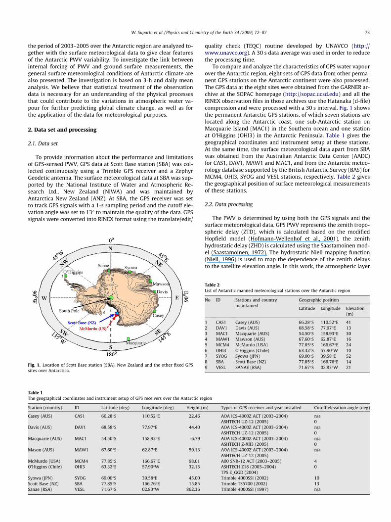
Fig. 1. Location of Scott Base station (SBA), New Zealand and the other fixed GPSsites over Antarctica.

Table 1The geographical coordinates and instrument setup of GPS receivers over the Antarctic re

Station (country) ID Latitude (deg) Longitude (deg) Height (m

Casey (AUS) CAS1 66.28�S 110.52�E 22.46

Davis (AUS) DAV1 68.58�S 77.97�E 44.40

Macquarie (AUS) MAC1 54.50�S 158.93�E -6.79

Mason (AUS) MAW1 67.60�S 62.87�E 59.13

McMurdo (USA) MCM4 77.85�S 166.67�E 98.01O’Higgins (Chile) OHI3 63.32�S 57.90�W 32.15

Syowa (JPN) SYOG 69.00�S 39.58�E 45.00Scott Base (NZ) SBA 77.85�S 166.76�E 15.85Sanae (RSA) VESL 71.67�S 02.83�W 862.36

quality check (TEQC) routine developed by UNAVCO (http://www.unavco.org). A 30 s data average was used in order to reducethe processing time.

To compare and analyze the characteristics of GPS water vapourover the Antarctic region, eight sets of GPS data from other perma-nent GPS stations on the Antarctic continent were also processed.The GPS data at the eight sites were obtained from the GARNER ar-chive at the SOPAC homepage (http://sopac.ucsd.edu) and all theRINEX observation files in those archives use the Hatanaka (d-file)compression and were processed with a 30 s interval. Fig. 1 showsthe permanent Antarctic GPS stations, of which seven stations arelocated along the Antarctic coast, one sub-Antarctic station onMacquarie Island (MAC1) in the Southern ocean and one stationat O’Higgins (OHI3) in the Antarctic Peninsula. Table 1 gives thegeographical coordinates and instrument setup at these stations.At the same time, the surface meteorological data apart from SBAwas obtained from the Australian Antarctic Data Center (AADC)for CAS1, DAV1, MAW1 and MAC1, and from the Antarctic meteo-rology database supported by the British Antarctic Survey (BAS) forMCM4, OHI3, SYOG and VESL stations, respectively. Table 2 givesthe geographical position of surface meteorological measurementsof these stations.

2.2. Data processing

The PWV is determined by using both the GPS signals and thesurface meteorological data. GPS PWV represents the zenith tropo-spheric delay (ZTD), which is calculated based on the modifiedHopfield model (Hofmann-Wellenhof et al., 2001), the zenithhydrostatic delay (ZHD) is calculated using the Saastamoinen mod-el (Saastamoinen, 1972). The hydrostatic Niell mapping function(Niell, 1996) is used to map the dependence of the zenith delaysto the satellite elevation angle. In this work, the atmospheric layer

gion

) Types of GPS receiver and year installed Cutoff elevation angle (deg)

AOA ICS-4000Z ACT (2003–2004) n/aASHTECH UZ-12 (2005) 0AOA ICS-4000Z ACT (2003–2004) n/aASHTECH UZ-12 (2005) 0AOA ICS-4000Z ACT (2003–2004) n/aASHTECH Z-XII3 (2005) 0AOA ICS-4000Z ACT (2003–2004) n/aASHTECH UZ-12 (2005)A00 SNR-12 ACT (2003–2005) 4ASHTECH Z18 (2003–2004) 0TPS E_GGD (2004)Trimble 4000SSI (2002) 10Trimble TS5700 (2002) 13Trimble 4000SSI (1997) n/a

Table 2List of Antarctic manned meteorological stations over the Antarctic region

No ID Stations and countrymaintained

Geographic position

Latitude Longitude Elevation(m)

1 CAS1 Casey (AUS) 66.28�S 110.52�E 412 DAV1 Davis (AUS) 68.58�S 77.97�E 133 MAC1 Macquarie (AUS) 54.50�S 158.93�E 304 MAW1 Mawson (AUS) 67.60�S 62.87�E 165 MCM4 McMurdo (USA) 77.85�S 166.67�E 246 OHI3 O’Higgins (Chile) 63.32�S 57.90�W 107 SYOG Syowa (JPN) 69.00�S 39.58�E 528 SBA Scott Base (NZ) 77.85�S 166.76�E 149 VESL SANAE (RSA) 71.67�S 02.83�W 21

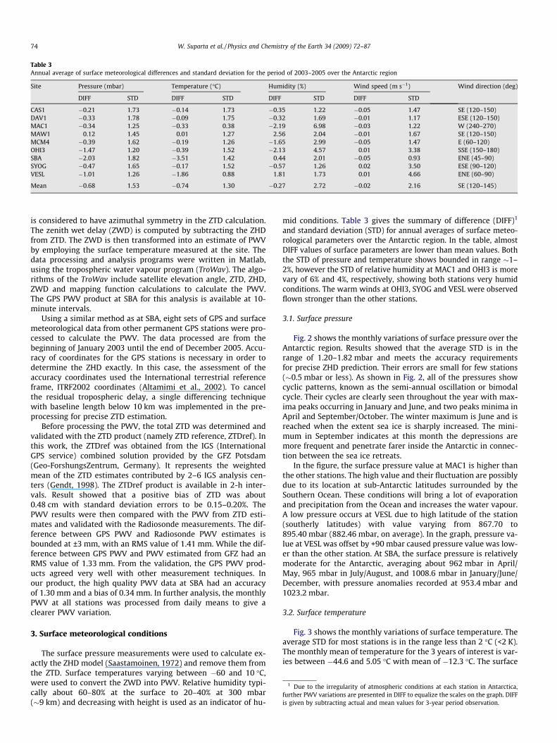
Table 3Annual average of surface meteorological differences and standard deviation for the period of 2003–2005 over the Antarctic region

Site Pressure (mbar) Temperature (�C) Humidity (%) Wind speed (m s�1) Wind direction (deg)

DIFF STD DIFF STD DIFF STD DIFF STD

CAS1 �0.21 1.73 �0.14 1.73 �0.35 1.22 �0.05 1.47 SE (120–150)DAV1 �0.33 1.78 �0.09 1.75 �0.32 1.69 �0.01 1.17 ESE (120–150)MAC1 �0.34 1.25 �0.33 0.38 �2.19 6.98 �0.03 1.22 W (240–270)MAW1 0.12 1.45 0.01 1.27 2.56 2.04 �0.01 1.67 SE (120–150)MCM4 �0.39 1.62 �0.19 1.26 �1.65 2.99 �0.05 1.47 E (60–120)OHI3 �1.47 1.20 �0.39 1.52 �2.13 4.57 0.01 3.38 SSE (150–180)SBA �2.03 1.82 �3.51 1.42 0.44 2.01 �0.05 0.93 ENE (45–90)SYOG �0.47 1.65 �0.17 1.52 �0.57 1.26 0.02 3.50 ESE (90–120)VESL �1.01 1.26 �1.86 0.88 1.81 1.73 0.01 4.66 ENE (60–90)

Mean �0.68 1.53 �0.74 1.30 �0.27 2.72 �0.02 2.16 SE (120–145)

1 Due to the irregularity of atmospheric conditions at each station in Antarctica,rther PWV variations are presented in DIFF to equalize the scales on the graph. DIFFgiven by subtracting actual and mean values for 3-year period observation.

74 W. Suparta et al. / Physics and Chemistry of the Earth 34 (2009) 72–87

is considered to have azimuthal symmetry in the ZTD calculation.The zenith wet delay (ZWD) is computed by subtracting the ZHDfrom ZTD. The ZWD is then transformed into an estimate of PWVby employing the surface temperature measured at the site. Thedata processing and analysis programs were written in Matlab,using the tropospheric water vapour program (TroWav). The algo-rithms of the TroWav include satellite elevation angle, ZTD, ZHD,ZWD and mapping function calculations to calculate the PWV.The GPS PWV product at SBA for this analysis is available at 10-minute intervals.

Using a similar method as at SBA, eight sets of GPS and surfacemeteorological data from other permanent GPS stations were pro-cessed to calculate the PWV. The data processed are from thebeginning of January 2003 until the end of December 2005. Accu-racy of coordinates for the GPS stations is necessary in order todetermine the ZHD exactly. In this case, the assessment of theaccuracy coordinates used the International terrestrial referenceframe, ITRF2002 coordinates (Altamimi et al., 2002). To cancelthe residual tropospheric delay, a single differencing techniquewith baseline length below 10 km was implemented in the pre-processing for precise ZTD estimation.

Before processing the PWV, the total ZTD was determined andvalidated with the ZTD product (namely ZTD reference, ZTDref). Inthis work, the ZTDref was obtained from the IGS (InternationalGPS service) combined solution provided by the GFZ Potsdam(Geo-ForshungsZentrum, Germany). It represents the weightedmean of the ZTD estimates contributed by 2–6 IGS analysis cen-ters (Gendt, 1998). The ZTDref product is available in 2-h inter-vals. Result showed that a positive bias of ZTD was about0.48 cm with standard deviation errors to be 0.15–0.20%. ThePWV results were then compared with the PWV from ZTD esti-mates and validated with the Radiosonde measurements. The dif-ference between GPS PWV and Radiosonde PWV estimates isbounded at ±3 mm, with an RMS value of 1.41 mm. While the dif-ference between GPS PWV and PWV estimated from GFZ had anRMS value of 1.33 mm. From the validation, the GPS PWV prod-ucts agreed very well with other measurement techniques. Inour product, the high quality PWV data at SBA had an accuracyof 1.30 mm and a bias of 0.34 mm. In further analysis, the monthlyPWV at all stations was processed from daily means to give aclearer PWV variation.

3. Surface meteorological conditions

The surface pressure measurements were used to calculate ex-actly the ZHD model (Saastamoinen, 1972) and remove them fromthe ZTD. Surface temperatures varying between �60 and 10 �C,were used to convert the ZWD into PWV. Relative humidity typi-cally about 60–80% at the surface to 20–40% at 300 mbar(�9 km) and decreasing with height is used as an indicator of hu-

mid conditions. Table 3 gives the summary of difference (DIFF)1

and standard deviation (STD) for annual averages of surface meteo-rological parameters over the Antarctic region. In the table, almostDIFF values of surface parameters are lower than mean values. Boththe STD of pressure and temperature shows bounded in range �1–2%, however the STD of relative humidity at MAC1 and OHI3 is morevary of 6% and 4%, respectively, showing both stations very humidconditions. The warm winds at OHI3, SYOG and VESL were observedflown stronger than the other stations.

3.1. Surface pressure

Fig. 2 shows the monthly variations of surface pressure over theAntarctic region. Results showed that the average STD is in therange of 1.20–1.82 mbar and meets the accuracy requirementsfor precise ZHD prediction. Their errors are small for few stations(�0.5 mbar or less). As shown in Fig. 2, all of the pressures showcyclic patterns, known as the semi-annual oscillation or bimodalcycle. Their cycles are clearly seen throughout the year with max-ima peaks occurring in January and June, and two peaks minima inApril and September/October. The winter maximum is June and isreached when the extent sea ice is sharply increased. The mini-mum in September indicates at this month the depressions aremore frequent and penetrate farer inside the Antarctic in connec-tion between the sea ice retreats.

In the figure, the surface pressure value at MAC1 is higher thanthe other stations. The high value and their fluctuation are possiblydue to its location at sub-Antarctic latitudes surrounded by theSouthern Ocean. These conditions will bring a lot of evaporationand precipitation from the Ocean and increases the water vapour.A low pressure occurs at VESL due to high latitude of the station(southerly latitudes) with value varying from 867.70 to895.40 mbar (882.46 mbar, on average). In the graph, pressure va-lue at VESL was offset by +90 mbar caused pressure value was low-er than the other station. At SBA, the surface pressure is relativelymoderate for the Antarctic, averaging about 962 mbar in April/May, 965 mbar in July/August, and 1008.6 mbar in January/June/December, with pressure anomalies recorded at 953.4 mbar and1023.2 mbar.

3.2. Surface temperature

Fig. 3 shows the monthly variations of surface temperature. Theaverage STD for most stations is in the range less than 2 �C (<2 K).The monthly mean of temperature for the 3 years of interest is var-ies between �44.6 and 5.05 �C with mean of �12.3 �C. The surface

fuis

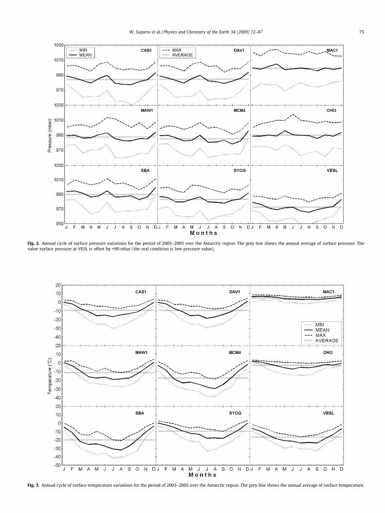
Fig. 2. Annual cycle of surface pressure variations for the period of 2003–2005 over the Antarctic region. The grey line shows the annual average of surface pressure. Thevalue surface pressure at VESL is offset by +90 mbar (the real condition is low pressure value).

Fig. 3. Annual cycle of surface temperature variations for the period of 2003–2005 over the Antarctic region. The grey line shows the annual average of surface temperature.

W. Suparta et al. / Physics and Chemistry of the Earth 34 (2009) 72–87 75

76 W. Suparta et al. / Physics and Chemistry of the Earth 34 (2009) 72–87

temperature at SBA was relative low for a sub-Antarctic, averagingabout �39 �C in July/August and 0.5 �C in January/December, withtemperature extremes recorded at �50.6 and 4 �C, respectively. Inthis observation, a high temperature (moderate to warm for Ant-arctic environment) was recorded at MAC1 with value vary from�8.8 to 12.5 �C and with a mean of 4.75 �C, followed by OHI3 from�1.5 to 3.3 �C and with a mean of 0.7 �C.

As shown in Fig. 3, a well-defined annual cycle was found to oc-cur for high plateau and coastal regions with larger values in sum-mer and smaller values in winter. Temperature passes betweenautumn and spring through two relative minima in April/Mayand August/September separated by a warming with a relativemaximum in June, which corresponds to the coreless winter result-ing from inversion of the temperature gradient variation. Noticethat the temperature starts to increase at the same time as thepressure reaches a minimum, showing the influence of the air ofoceanic origin brought by the depressions. The temperature in-crease in spring is faster than during autumn. Remarkably, thetemperature conditions at all stations are closely related with ele-vation and drop rapidly inland of the coast to low-level tempera-ture (rise of temperature with increasing elevation), as wasstudied by van Lipzig et al. (2002).

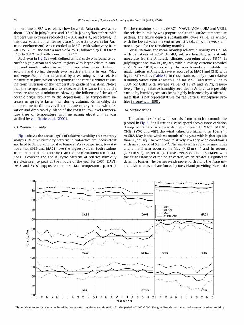
3.3. Relative humidity

Fig. 4 shows the annual cycle of relative humidity on a monthlyanalysis. Relative humidity patterns in Antarctica are inconsistentand hard to define: unimodal or bimodal. As a comparison, two sta-tions that OHI3 and MAC1 have the highest values. Both stationsare more humid and unstable than the main continent (coast sta-tions). However, the annual cycle patterns of relative humidityare clear seen to peak at the middle of the year for CAS1, DAV1,OHI3 and SYOG (opposite to the surface temperature pattern).

Fig. 4. Mean monthly of relative humidity variations over the Antarctic region for the

For the remaining stations (MAC1, MAW1, MCM4, SBA and VESL),the relative humidity was proportional to the surface temperaturepattern. The figure depicts substantially lower values in winter,with the lowest value (in September) at VESL, all with a weak uni-modal cycle for the remaining months.

For all stations, the mean monthly relative humidity was 71.4%with deviations of ±20%. At SBA, relative humidity is relativelymoderate for the Antarctic climate, averaging about 56.7% inJuly/August and 96% in Jan/Dec, with humidity extreme recordedat 20.5% and 101%, respectively. The more humid and unstable cli-matic stations at Antarctica were recorded at MAC1 and OHI3 withhigher STD values (Table 3). In those stations, daily mean relativehumidity varies from 43.6% to 105% for MAC1 and from 29.5% to100% for OHI3 with average values of 87.2% and 89.7%, respec-tively. The high relative humidity recorded in Antarctica is possiblycaused by humidity sensors being highly influenced by a microcli-mate that is not representatives for the vertical atmosphere pro-files (Bromwich, 1990).

3.4. Surface winds

The annual cycle of wind speeds from month-to-month areplotted in Fig. 5. At all stations, wind speed shows more variationduring winter and is slower during summer. At MAC1, MAW1,OHI3, SYOG and VESL the wind values are higher than 10 m s�1.At SBA, May is the windiest month of the year with higher speedsthan in January. The wind was relatively low (dry wind conditions)with mean speed of 5.2 m s�1. The winds with a relative maximumand a minimum occurred in May (�15 m s�1) and in August(�0.4 m s�1), respectively. These events can be associated withthe establishment of the polar vortex, which creates a significantdynamic barrier. The barrier winds move north along the Transant-arctic Mountains and are forced by Ross Island providing McMurdo

period of 2003–2005. The grey line shows the annual average relative humidity.

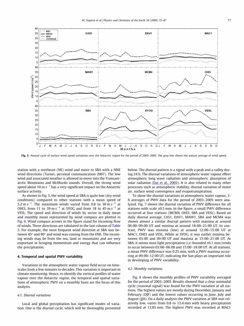
Fig. 5. Annual cycle of surface wind speed variations over the Antarctic region for the period of 2003–2005. The grey line shows the annual average of wind speed.

W. Suparta et al. / Physics and Chemistry of the Earth 34 (2009) 72–87 77

station with a northeast (NE) wind and move to SBA with a NNEwind directions (Turner, personal communication 2007). The lowwind and associated weather is allowed to move into the Transant-arctic Mountains and McMurdo sounds. Overall, the strong windspeed about 10 m s�1 has a very significant impact on the Antarcticsurface activity.

As shown in Fig. 5, the wind speed at SBA is quite low (dry windconditions) compared to other stations with a mean speed of5.2 m s�1. The maximum winds varied from 9.8 to 38 m s�1 atOHI3, from 11 to 39 m s�1 at SYOG and from 18 to 45 m s�1 atVESL. The speed and direction of winds by sector in daily meanand monthly mean represented by wind compass are plotted inFig. 6. Wind compass arrows in the figure stand for incoming flowof winds. These directions are tabulated in the last column of Table3. For example, the most frequent wind direction at SBA was be-tween 45� and 90� and wind was coming from the ENE. The incom-ing winds may be from the sea, land or mountains and are veryimportant in bringing momentum and energy that can influencethe precipitation.

4. Temporal and spatial PWV variability

Variations in the atmospheric water vapour field occur on time-scales from a few minutes to decades. This variation is important inclimate monitoring. Hence, to identify the vertical profiles of watervapour over the Antarctic region, the temporal and spatial varia-tions of atmospheric PWV on a monthly basis are the focus of thisanalysis.

4.1. Diurnal variations

Local and global precipitation has significant modes of varia-tion. One is the diurnal cycle, which will be thoroughly presented

below. The diurnal pattern is a signal with a peak and a valley dur-ing 24 h. The diurnal variations of atmospheric water vapour effectatmospheric long wave radiation and atmospheric absorption ofsolar radiation (Dai et al., 2002). It is also related to many otherprocesses such as atmospheric stability, diurnal variation of moistair, surface wind convergence and evapotranspiration.

To show the diurnal variations in atmospheric water vapour, 3-h averages of PWV data for the period of 2003–2005 were ana-lyzed. Fig. 7 shows the diurnal variation of PWV difference for allstations with scale ±0.5 mm. In the figure, a small PWV differenceoccurred at four stations (MCM4, OHI3, SBA and VESL). Based ondaily diurnal average, CAS1, DAV1, MAW1, SBA and MCM4 wasshown almost a similar diurnal pattern with maxima at around06:00–09:00 UT and minima at around 18:00–21:00 UT. In con-trast, PWV was minima (low) at around 12:00–15:00 UT atMAC1, OHI3 and VESL. While at SYOG, it was earlier minima be-tween 03:00 and 09:00 UT and maxima at 15:00–21:00 UT. AtSBA, it seems most light precipitation (i.e. bounded ±0.1 mm) tendsto occur between 03:00–06:00 and 15:00–18:00 UT. At all stations,a mean PWV difference was 0.25 mm, with a PWV maxima occur-ring at 09:00–12:00 UT, indicating the Sun plays an important rolein developing of PWV variability.

4.2. Monthly variations

Fig. 8 shows the monthly profiles of PWV variability averagedfor the period of 2003–2005. Results showed that a clear unimodalcycle (seasonal signal) was found for the PWV variation at all sta-tions. The highest values are mostly during December, January andFebruary (DJF) and the lowest values occurring in June, July andAugust (JJA). On a daily analysis the PWV variation at SBA was rel-atively low, varies from 0.8 to 13.4 mm with heavy precipitationrecorded at 13.85 mm. The highest PWV was recorded at MAC1

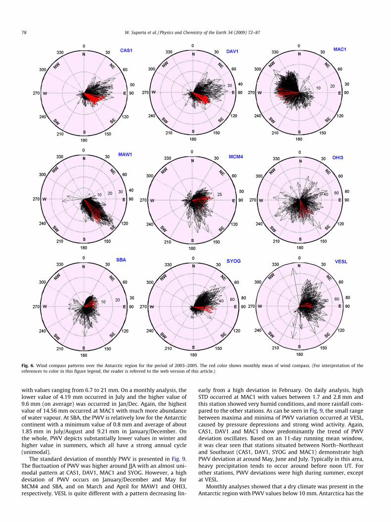
Fig. 6. Wind compass patterns over the Antarctic region for the period of 2003–2005. The red color shows monthly mean of wind compass. (For interpretation of thereferences to color in this figure legend, the reader is referred to the web version of this article.)

78 W. Suparta et al. / Physics and Chemistry of the Earth 34 (2009) 72–87

with values ranging from 6.7 to 21 mm. On a monthly analysis, thelower value of 4.19 mm occurred in July and the higher value of9.6 mm (on average) was occurred in Jan/Dec. Again, the highestvalue of 14.56 mm occurred at MAC1 with much more abundanceof water vapour. At SBA, the PWV is relatively low for the Antarcticcontinent with a minimum value of 0.8 mm and average of about1.85 mm in July/August and 9.21 mm in January/December. Onthe whole, PWV depicts substantially lower values in winter andhigher value in summers, which all have a strong annual cycle(unimodal).

The standard deviation of monthly PWV is presented in Fig. 9.The fluctuation of PWV was higher around JJA with an almost uni-modal pattern at CAS1, DAV1, MAC1 and SYOG. However, a highdeviation of PWV occurs on January/December and May forMCM4 and SBA, and on March and April for MAW1 and OHI3,respectively. VESL is quite different with a pattern decreasing lin-

early from a high deviation in February. On daily analysis, highSTD occurred at MAC1 with values between 1.7 and 2.8 mm andthis station showed very humid conditions, and more rainfall com-pared to the other stations. As can be seen in Fig. 9, the small rangebetween maxima and minima of PWV variation occurred at VESL,caused by pressure depressions and strong wind activity. Again,CAS1, DAV1 and MAC1 show predominantly the trend of PWVdeviation oscillates. Based on an 11-day running mean window,it was clear seen that stations situated between North–Northeastand Southeast (CAS1, DAV1, SYOG and MAC1) demonstrate highPWV deviation at around May, June and July. Typically in this area,heavy precipitation tends to occur around before noon UT. Forother stations, PWV deviations were high during summer, exceptat VESL.

Monthly analyses showed that a dry climate was present in theAntarctic region with PWV values below 10 mm. Antarctica has the

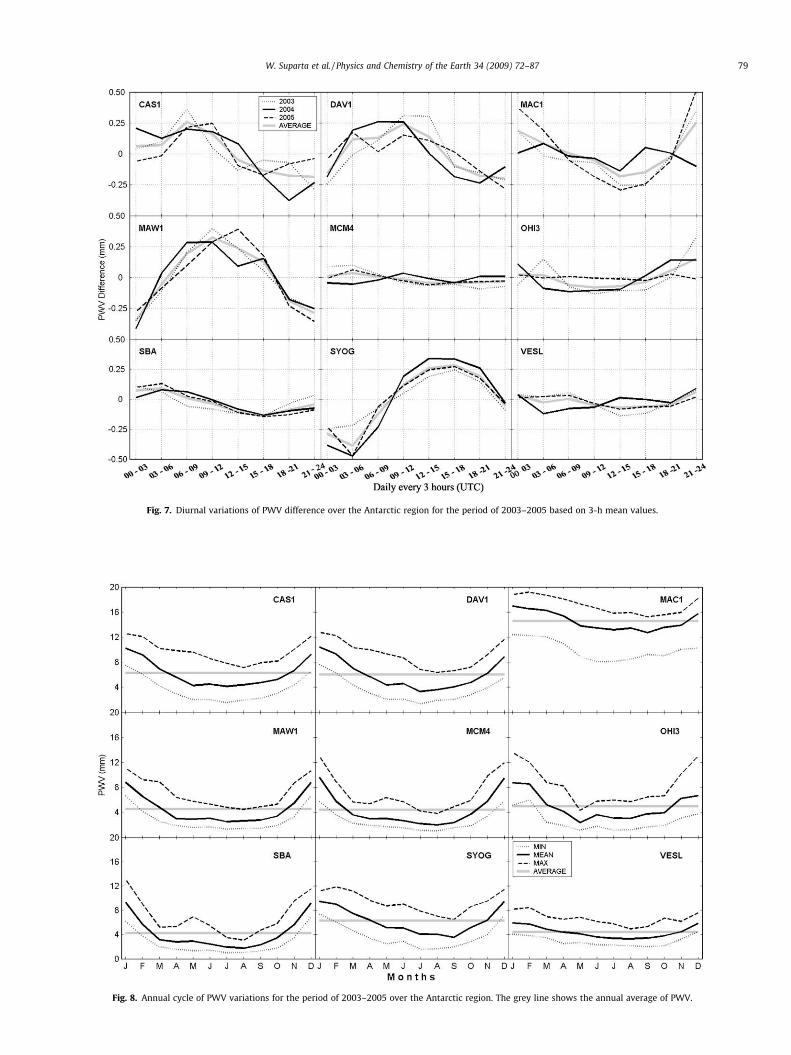
Fig. 7. Diurnal variations of PWV difference over the Antarctic region for the period of 2003–2005 based on 3-h mean values.

Fig. 8. Annual cycle of PWV variations for the period of 2003–2005 over the Antarctic region. The grey line shows the annual average of PWV.

W. Suparta et al. / Physics and Chemistry of the Earth 34 (2009) 72–87 79

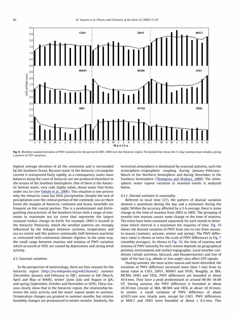
Fig. 9. Monthly standard deviation of PWV variations for the period of 2003–2005 over the Antarctic region. The dashed line shows the 11-day running mean window, givinga pattern of STD variations.

80 W. Suparta et al. / Physics and Chemistry of the Earth 34 (2009) 72–87

highest average elevation of all the continents and is surroundedby the Southern Ocean. Because water in the Antarctic circumpolarcurrent is transported fairly rapidly, as a consequence, water massbalances along the coast of Antarctic are not produced elsewhere inthe oceans of the Southern hemisphere. One of these is the Antarc-tic bottom water, very cold, highly saline, dense water that formsunder sea ice (see Yabuki et al., 2006). This situation is one processwhy the Antarctic coast has little precipitation. Despite the lack ofprecipitation over the central portion of the continent, sea ice thereforms the margins of Antarctic continent and heavy snowfalls arefrequent on the coastal portion. This is a predominant and distin-guishing characteristic of the Southern Ocean with a range of min-imum to maximum sea ice cover that represents the largestseasonal surface change on Earth. For example, OHI3 is located inthe Antarctic Peninsula, which the weather patterns are stronglyinfluenced by the linkages between cyclones, temperature andsea ice extent and this pattern continually shift between maritimeas contrasted with continental climatic regimes. In the same way,the small range between maxima and minima of PWV variationwhich occurred at VESL are caused by depressions and strong windactivity.

4.3. Seasonal variations

In the perspective of meteorology, there are four seasons for theAntarctic region (http://en.wikipedia.org/wiki/Season): summer(December, January and February or DJF), autumn or fall (March,April and May or MAM), winter (June, July and August or JJA)and spring (September, October and November or SON). These sea-sons clearly show that in the Antarctic region, the relationship be-tween the solar activity and the water vapour peaks in summer.Temperature changes are greatest in summer months, but relativehumidity changes are pronounced in winter months. Similarly, the

terrestrial atmosphere is dominated by seasonal patterns, such thestratosphere–troposphere coupling during January–February–March in the Northern hemisphere and during November in theSouthern hemisphere (Thompson and Wallace, 2000). The atmo-spheric water vapour variation in seasonal events is analyzedbelow.

4.3.1. Diurnal variation in seasonalityReferred to local time (LT), the pattern of diurnal variation

showed a maximum during the day and a minimum during thenight. Within the accuracy afforded by a 3-h average, there is somechange in the time of maxima from 2003 to 2005. The grouping ofmonths into seasons causes some change in the time of maxima.The times have been examined separately for each month to deter-mine which interval is a maximum the majority of time. Fig. 10shows the diurnal variation of PWV from site-to-site from season-to-season (summer, autumn, winter and spring). The PWV differ-ence value is shown at twice the scale of PWV differences in Fig. 7(monthly averages). As shown in Fig. 10, the time of maxima andminima of PWV intensity for each station depends on geographicalposition, environment and surface topographic. Local weather con-ditions (winds activities, blizzard, and thunderstorms) and line ofsight of the Sun (e.g. albedo or Sun angle) also affect GPS signals.

During summer, the most active season and more disturbed, thevariation of PWV difference increased more than 1 mm from itsmean value at CAS1, DAV1, MAW1 and SYOG. Roughly, at SBA,MCM4, OHI3 and VESL, PWV differences are bounded at about±0.4 mm. They have a peak predominant at around 06:00–18:00UT. During autumn, the PWV difference is bounded at about±0.30 mm (except at SBA, MCM4 and VESL at about ±0.10 mm).In winter, a small variation of PWV difference of about±0.025 mm was clearly seen, except for CAS1. PWV differencesat MAC1 and OHI3 were bounded at about ± 0.2 mm. This

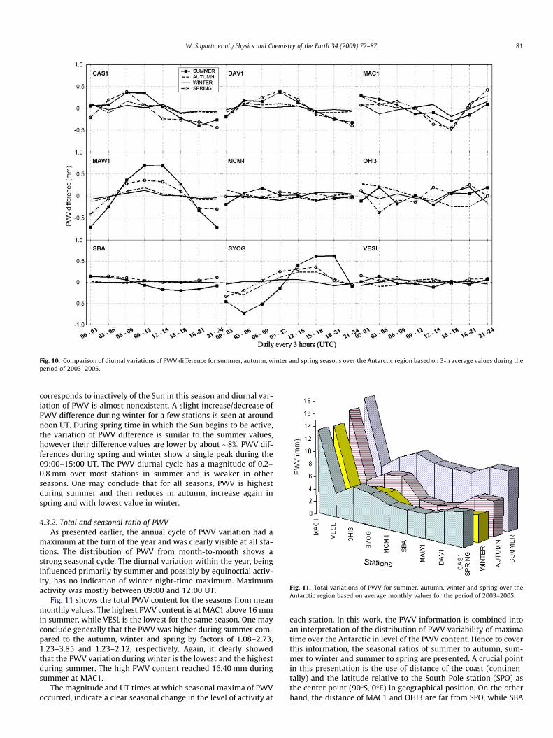
Fig. 10. Comparison of diurnal variations of PWV difference for summer, autumn, winter and spring seasons over the Antarctic region based on 3-h average values during theperiod of 2003–2005.

Fig. 11. Total variations of PWV for summer, autumn, winter and spring over theAntarctic region based on average monthly values for the period of 2003–2005.

W. Suparta et al. / Physics and Chemistry of the Earth 34 (2009) 72–87 81

corresponds to inactively of the Sun in this season and diurnal var-iation of PWV is almost nonexistent. A slight increase/decrease ofPWV difference during winter for a few stations is seen at aroundnoon UT. During spring time in which the Sun begins to be active,the variation of PWV difference is similar to the summer values,however their difference values are lower by about �8%. PWV dif-ferences during spring and winter show a single peak during the09:00–15:00 UT. The PWV diurnal cycle has a magnitude of 0.2–0.8 mm over most stations in summer and is weaker in otherseasons. One may conclude that for all seasons, PWV is highestduring summer and then reduces in autumn, increase again inspring and with lowest value in winter.

4.3.2. Total and seasonal ratio of PWVAs presented earlier, the annual cycle of PWV variation had a

maximum at the turn of the year and was clearly visible at all sta-tions. The distribution of PWV from month-to-month shows astrong seasonal cycle. The diurnal variation within the year, beinginfluenced primarily by summer and possibly by equinoctial activ-ity, has no indication of winter night-time maximum. Maximumactivity was mostly between 09:00 and 12:00 UT.

Fig. 11 shows the total PWV content for the seasons from meanmonthly values. The highest PWV content is at MAC1 above 16 mmin summer, while VESL is the lowest for the same season. One mayconclude generally that the PWV was higher during summer com-pared to the autumn, winter and spring by factors of 1.08–2.73,1.23–3.85 and 1.23–2.12, respectively. Again, it clearly showedthat the PWV variation during winter is the lowest and the highestduring summer. The high PWV content reached 16.40 mm duringsummer at MAC1.

The magnitude and UT times at which seasonal maxima of PWVoccurred, indicate a clear seasonal change in the level of activity at

each station. In this work, the PWV information is combined intoan interpretation of the distribution of PWV variability of maximatime over the Antarctic in level of the PWV content. Hence to coverthis information, the seasonal ratios of summer to autumn, sum-mer to winter and summer to spring are presented. A crucial pointin this presentation is the use of distance of the coast (continen-tally) and the latitude relative to the South Pole station (SPO) asthe center point (90�S, 0�E) in geographical position. On the otherhand, the distance of MAC1 and OHI3 are far from SPO, while SBA

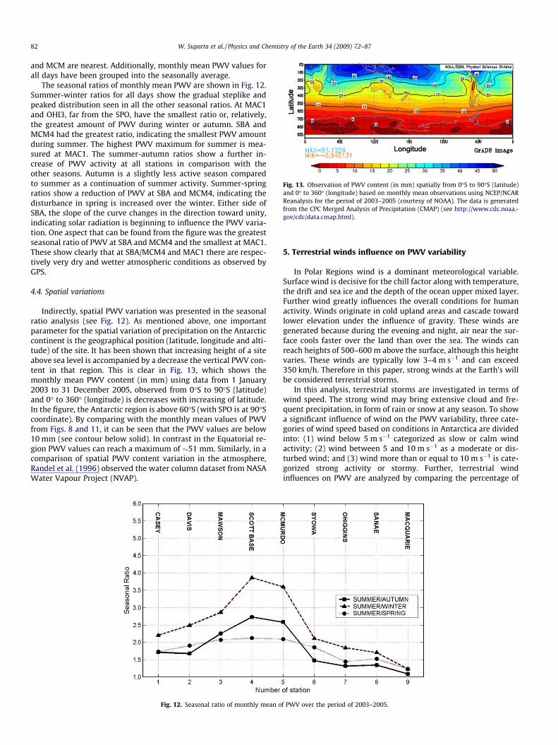
Fig. 13. Observation of PWV content (in mm) spatially from 0�S to 90�S (latitude)and 0� to 360� (longitude) based on monthly mean observations using NCEP/NCARReanalysis for the period of 2003–2005 (courtesy of NOAA). The data is generatedfrom the CPC Merged Analysis of Precipitation (CMAP) (see http://www.cdc.noaa.-gov/cdc/data.cmap.html).

82 W. Suparta et al. / Physics and Chemistry of the Earth 34 (2009) 72–87

and MCM are nearest. Additionally, monthly mean PWV values forall days have been grouped into the seasonally average.

The seasonal ratios of monthly mean PWV are shown in Fig. 12.Summer-winter ratios for all days show the gradual steplike andpeaked distribution seen in all the other seasonal ratios. At MAC1and OHI3, far from the SPO, have the smallest ratio or, relatively,the greatest amount of PWV during winter or autumn. SBA andMCM4 had the greatest ratio, indicating the smallest PWV amountduring summer. The highest PWV maximum for summer is mea-sured at MAC1. The summer-autumn ratios show a further in-crease of PWV activity at all stations in comparison with theother seasons. Autumn is a slightly less active season comparedto summer as a continuation of summer activity. Summer-springratios show a reduction of PWV at SBA and MCM4, indicating thedisturbance in spring is increased over the winter. Either side ofSBA, the slope of the curve changes in the direction toward unity,indicating solar radiation is beginning to influence the PWV varia-tion. One aspect that can be found from the figure was the greatestseasonal ratio of PWV at SBA and MCM4 and the smallest at MAC1.These show clearly that at SBA/MCM4 and MAC1 there are respec-tively very dry and wetter atmospheric conditions as observed byGPS.

4.4. Spatial variations

Indirectly, spatial PWV variation was presented in the seasonalratio analysis (see Fig. 12). As mentioned above, one importantparameter for the spatial variation of precipitation on the Antarcticcontinent is the geographical position (latitude, longitude and alti-tude) of the site. It has been shown that increasing height of a siteabove sea level is accompanied by a decrease the vertical PWV con-tent in that region. This is clear in Fig. 13, which shows themonthly mean PWV content (in mm) using data from 1 January2003 to 31 December 2005, observed from 0�S to 90�S (latitude)and 0� to 360� (longitude) is decreases with increasing of latitude.In the figure, the Antarctic region is above 60�S (with SPO is at 90�Scoordinate). By comparing with the monthly mean values of PWVfrom Figs. 8 and 11, it can be seen that the PWV values are below10 mm (see contour below solid). In contrast in the Equatorial re-gion PWV values can reach a maximum of �51 mm. Similarly, in acomparison of spatial PWV content variation in the atmosphere,Randel et al. (1996) observed the water column dataset from NASAWater Vapour Project (NVAP).

Fig. 12. Seasonal ratio of monthly mean o

5. Terrestrial winds influence on PWV variability

In Polar Regions wind is a dominant meteorological variable.Surface wind is decisive for the chill factor along with temperature,the drift and sea ice and the depth of the ocean upper mixed layer.Further wind greatly influences the overall conditions for humanactivity. Winds originate in cold upland areas and cascade towardlower elevation under the influence of gravity. These winds aregenerated because during the evening and night, air near the sur-face cools faster over the land than over the sea. The winds canreach heights of 500–600 m above the surface, although this heightvaries. These winds are typically low 3–4 m s�1 and can exceed350 km/h. Therefore in this paper, strong winds at the Earth’s willbe considered terrestrial storms.

In this analysis, terrestrial storms are investigated in terms ofwind speed. The strong wind may bring extensive cloud and fre-quent precipitation, in form of rain or snow at any season. To showa significant influence of wind on the PWV variability, three cate-gories of wind speed based on conditions in Antarctica are dividedinto: (1) wind below 5 m s�1 categorized as slow or calm windactivity; (2) wind between 5 and 10 m s�1 as a moderate or dis-turbed wind; and (3) wind more than or equal to 10 m s�1 is cate-gorized strong activity or stormy. Further, terrestrial windinfluences on PWV are analyzed by comparing the percentage of

f PWV over the period of 2003–2005.

W. Suparta et al. / Physics and Chemistry of the Earth 34 (2009) 72–87 83

PWV difference between disturbed and stormy with respect tothe calm (slow) wind. The percentage PWV difference is definedas

%DPWV ¼ PWVj � PWVq

PWVq� 100% ð1Þ

where j = a, b is the PWV for disturbed (a) and stormy (b), and q isthe PWV during slow wind activity.

Fig. 14 shows the time series of PWV superimposed for thethree activities of winds above. In the figure, the monthly percent-age of %DPWV with strong wind (stormy) was shown decreasedthe PWV, except at MAC1, OHI3 and VESL. More positive value of%DPWV is more decreased the PWV as strongest wind speed. Thewind speed observed at VESL (see Fig. 5) was noticeably strongerthat those at the coast for the period of 2003–2005, sustainedwinds greater than 50 m s�1. From Table 3, VESL was the windieststation with the biggest of STD of 4.66 m s�1 and an annual meanspeed of �20 m s�1. The airflow displays a strong easterly compo-nent with 52% of the wind blowing from East. In this station, pre-cipitation is almost very rarely observed during summer month.The most significant precipitation events are associated with thepassage of deep depressions near the station. A strong annualmean speed was observed at OHI3 exceeding 13 m s�1. This stationlocated at Western Antarctic Peninsula, which is strongly affectedby depression of low pressure and has predominantly warm windfrom the Northeast to cold dry continental conditions with South-westerly winds. At MAC1, the wind is affected by the persistentwesterly belts that sweep over the Southern ocean and 70% indirection blow between SE and NW throughout the year. Thuswind activity at this station has only small effects on the PWV dis-tribution. At all stations, decreasing PWV variations with strongwinds are clearly seen in winter.

Fig. 14. Monthly profiles of percentage PWV difference between disturbed and stormy r2005.

The second investigation of terrestrial wind influence on PWV isanalyzed through their diurnal variation with season. Fig. 15 showsthe diurnal variations of wind speed and PWV differences. In thebottom of each panel in Fig. 14 is shown the correlation coefficient(r) between wind speed and PWV, which are all significant at the99% confidence levels. The statistical significance for each parame-ter at every time point at four seasons and from site-to-sitehas been tested using Student’s t test and the results is shown inTable 4. During summer, both variations of PWV and wind speeddifferences from site-to-site are highest compared to the other sea-sons. Their ratios and total values (see Figs. 11 and 12) are almosttwice those in the other seasons. The highest value occurred atMAC1. Strong negative correlations between PWV and wind differ-ences with season occur at CAS1, MAW1, MCM4, SBA and SYOG(see Fig. 15a), indicating warm wind potentially decreasing thePWV content. During autumn when the precipitation starts to de-crease, the inverse relationship between wind and PWV is seen atall stations. While during winter, their correlation not so strong butstill opposite to each other. Differing from autumn and winter sea-sons, the spring season showed the correlation between wind andPWV increased progressively, except at MAC1 and VESL. At MAC1,the PWV difference tends to increase with changing wind activityalthough the correlation was weak. As presented in Table 4, the ra-tio between PWV and wind speed at MAC1 was higher for all sea-sons. The biggest value of wind with lowest water vapour wasrecorded at VESL. The lowest precipitation amounts spatially atAntarctica are due to lack of synoptic forcing and conditions of sur-face slope or topographical/geographical parameters (van Lipziget al., 2002). As noticed by van Lipzig et al., the elevated terrain actsto block the penetration of synoptic disturbances onto the plateau,when the slope is steep and the large-scale wind is directed ups-lope, the rising air results in enhanced precipitation. Precipitation

espect to the calm winds activities over the Antarctic region for the period of 2003–

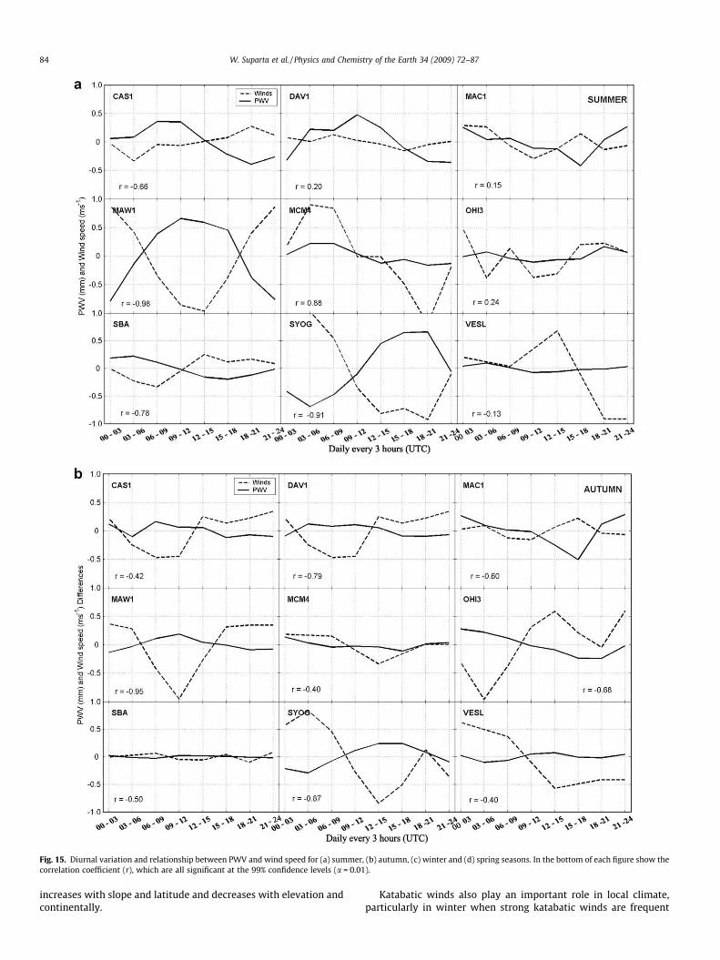
Fig. 15. Diurnal variation and relationship between PWV and wind speed for (a) summer, (b) autumn, (c) winter and (d) spring seasons. In the bottom of each figure show thecorrelation coefficient (r), which are all significant at the 99% confidence levels (a = 0.01).

84 W. Suparta et al. / Physics and Chemistry of the Earth 34 (2009) 72–87

increases with slope and latitude and decreases with elevation andcontinentally.

Katabatic winds also play an important role in local climate,particularly in winter when strong katabatic winds are frequent

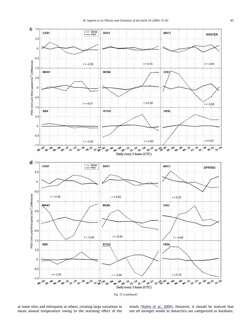
Fig. 15 (continued)

W. Suparta et al. / Physics and Chemistry of the Earth 34 (2009) 72–87 85

at some sites and infrequent at others, creating large variations inmean annual temperature owing to the warming effect of the

winds (Nylen et al., 2004). However, it should be noticed thatnot all stronger winds in Antarctica are categorized as katabatic.

Table 4Ratio between PWV and wind speed and its correlation strength

Site Summer Autumn Winter Spring Annual

CAS1 1.45 (M) 0.83 (M) 0.58 (M) 0.66 (M) 0.88DAV1 1.50 (N) 0.84 (S) 0.59 (N) 0.75 (M) 0.92MAC1 1.87 (N) 1.38 (M) 1.28 (N) 1.36 (N) 1.47MAW1 0.83 (S) 0.27 (S) 0.21 (N) 0.30 (S) 0.40MCM4 0.75 (S) 0.43 (M) 0.40 (M) 0.43 (M) 0.50OHI3 0.87 (N) 0.67 (M) 0.44 (M) 0.53 (M) 0.63SBA 1.54 (S) 0.47 (M) 0.32 (N) 0.63 (M) 0.74SYOG 0.89 (S) 0.38 (S) 0.29 (M) 0.40 (S) 0.49VESL 0.37 (N) 0.21 (M) 0.16 (M) 0.20 (N) 0.23

Mean 1.21 0.66 0.51 0.63 0.75

Note: N, M and S are stands for the (N)o, (M)oderate and (S)trong correlationsrespectively with guideline 0 < |r| < 0.30 (N), 0.30 < |r| < 0.70 (M) and |r| > 0.70 (S)were analyzed from Fig. 13.

86 W. Suparta et al. / Physics and Chemistry of the Earth 34 (2009) 72–87

As discussed by Parish (personal communication, 2006), katabaticwinds descend down a mountain slope (in the valleys of the Tran-santarctic mountains), and are generally much stronger thanmountain breezes.

6. Summary and conclusions

There are two main themes in this paper. First, the analysis ofthe characteristics of GPS-sensed PWV over the Antarctic region,and, second the investigation of terrestrial wind influence onPWV. The analyses focused on temporal and spatial variations.The outcomes are summarized as follows. The atmospheric watervapour shows significant variability over time and space. Atmo-spheric water vapour shows large seasonal changes with a maxi-mum in summer and a minimum in winter. Specifically, thetrend in the variation of PWV over the year was similar to theso-called annual cycle or unimodal pattern. Seasonal analysisshowed that the summer season had the greatest variability ofall seasons. Spring is more variable than autumn, and during sum-mer the temperatures remain close to the climatic average temper-atures. The PWV variation during the winter is relatively poorlycharacterized and the standard deviation was higher, suggestinglarger relative errors in situations with low water vapour amounts.In winter, the temperature increase was lower by about 1 �C andvalues of water vapour were 13% smaller than during summermonths. The PWV minimum was associated with the cold airadvection during winter. The summer periods are of particularinterest for regions like Antarctica, when warm temperatures withhigh PWV values, together with strong cumulus convection resultin precipitation. Water vapour also shows large diurnal variationand there are diurnal variations in precipitation. Evidently, solaractivity affects the GPS-sensed PWV. PWV in Antarctica was below10 mm with STD ranging from 0.5 to 2.8 mm. The lower PWVamount was caused by dry atmospheric conditions in those re-gions. SBA has the driest Antarctic climate among the other sta-tions in this analysis. From the point of view of meteorology, itseems that the most extreme and driest months at SBA are Mayand August respectively, and that January is the best month ofthe year for travel and other human activities. Overall, the charac-teristics of Antarctic climate representing by the PWV variationshow a seasonal dependence, highest (active) in summer and low-est (inactive) in winter.

Wind energy originating from solar activity can increase or de-crease the PWV distribution. An investigation of terrestrial windinfluence on PWV gave the following outcomes. The large decreasein PWV in the monthly mean value was accompanied by strongwinds above 10 m s�1. The inversion is strongest in winter, asshown by the percentage of PWV and wind speed differences. In

contrast, it seems that the summer months are not the least windymonths of the year. In summer and spring seasons, the PWV mag-nitude was almost twice as large as in the winter season. Strongwinds potentially decreased the precipitation. The passage deepdepression is a major contributor. The other possibilities for lowprecipitation in Antarctica are lack of synoptic forcing and surfaceslope or topographical/geographical parameters (van Lipzig et al.,2002). It was shown that the majority diurnal changes in PWVare negatively correlated with wind speed differences. The influ-ence of katabatic wind on the PWV variability and the GPS signalsremain topics of further interest. The possibility of katabatic eventsdecreases or increasing the PWV content using GPS, remain atopic of future studies. Overall, the PWV data quality was goodin temporal resolution. The data will be of benefit for climate mon-itoring as well as data assimilation for numerical weatherprediction.

Acknowledgements

This research was supported by the Academy of SciencesMalaysia under the ANZ K141B grant through Ministry of Science,Technology and Innovation Malaysia (MOSTI) and Universiti Ke-bangsaan Malaysia. The authors would like to express their grati-tude to Dr. Dean Peterson and the managerial staff and sciencetechnicians of Antarctica New Zealand (ANZ) and Andrew R. Har-per at the National Institute of Water and Atmospheric ResearchLtd., New Zealand (NIWA) for maintaining the GPS and surfacemeteorological measurements, and supporting this work. Wewould also like to thank to the Scripps Orbit and Permanent ArrayCenter (SOPAC) for archiving the GPS data from the dense globalnetwork, the Australian Antarctic Data Center (AADC) and the Brit-ish Antarctic Survey (BAS) for providing the surface meteorologicaldata.

References

Altamimi, Z., Sillard, P., Boucher, C., 2002. ITRF2000: A new release of theinternational terrestrial reference frame for earth science applications. J.Geophys. Res. 107 (B10), 2214, doi:10.1029/2001JB000561.

Bevis, M., Businger, S., Herring, T.A., Rocken, C., Anthes, R.A., Ware, R.H., 1992. GPSmeteorology: remote sensing of atmospheric water vapor using the globalpositioning system. J. Geophys. Res. 97 (D14), 15787–15801.

Bromwich, H.D., 1990. Estimates of Antarctic precipitation. Nature 343, 627–629.Coster, A.A., Niell, A., Solheim, F., Mendes, V., Toor, P., Langley, R., Ruggles, C., 1996.

The westford water vapour experiment: use of GPS to determine totalprecipitable water vapour. In: Proceeding of Institute of Navigation 52ndAnnual Meeting, Cambridge, MA, USA, 19–21 June, pp. 529–538.

Dai, A., Wang, J., Ware, R.H., Van Hove, T., 2002. Diurnal variation in water vaporover North America and its implications for sampling errors in radiosondehumidity. J. Geophys. Res 107 (D10), 4090, doi:10.1029/2001JD000642.

Duan, J., Bevis, M., Fang, P., Bock, Y., Chiswell, S., Businger, S., Rocken, C., Solheim, F.,van Hove, T., Ware, R., McClusky, S., Herring, T.A., King, R.W., 1996. GPSmeteorology: Direct estimation of the absolute value of precipitable water. J.Appl. Meteorol. 35 (6), 830–838.

Gaffen, D.J., Barnett, T.P., Elliot, W.P., 1991. Space and time scales of globaltropospheric moisture. J. Clim. 4, 989–1008.

Gendt, G., 1998. IGS combination of tropospheric estimates – experience from pilotproject. Proc. IGS Analysis Centre Workshop, Darmstadt.

Gendt, G., Dick, G., Reigber, C., Tomassini, M., Liu, Y., Ramatschi, M., 2004. Near realtime GPS water vapour monitoring for numerical weather prediction atGermany. J. Meteorol. Soc. Jpn. 82, 361–370.

Gradinarsky, L.P., Johansson, J.M., Bouma, H.R., Scherneck, H.-G., Elgered, G., 2002.Climate monitoring using GPS. Phys. Chem. Earth 27, 335–340.

Guerova, G., Brockmann, E., Quiby, J., Schubiger, F., Matzler, C., 2003. Validation ofNWP models with Swiss GPS network AGNES. J. Appl. Meteorol. 42, 141–150.

Hofmann-Wellenhof, B., Lichtenegger, H., Collins, J., 2001. Global PositioningSystem: Theory and Practice, seventh ed. Springer Verlag, New York.

Kuo, Y.H., Guo, Y.R., Westwater, E.R., 1993. Assimilation of precipitable watermeasurements into a mesoscale and numerical model. Mon. Weather Rev. 121,1215–1238.

Liou, Y.A., Teng, Y.T., van Hove, T., Liljegren, J.C., 2001. Comparison of precipitablewater observations in the near tropics by GPS, microwave radiometer andradiosondes. J. Appl. Meteorol. 40 (1), 5–15.

Manabe, S., Wetherald, R., 1967. Thermal equilibrium of the atmosphere with agiven distribution of relative humidity. J. Atmos. Sci 24, 241–259.

W. Suparta et al. / Physics and Chemistry of the Earth 34 (2009) 72–87 87

Mockler, S.B. 1995. Water vapour in the climate system. Special report, Americangeophysical Union (AGU), 2000 Florida Ave, N.W., Washington, DC 20009,December, ISBN 0-87590-865-9. <http://www.agu.org/sci_soc/mockler.html>.

Niell, A.E., 1996. Global mapping functions for the atmosphere delay at radiowavelengths. J. Geophys. Res. 101 (B2), 3197–3246.

Nylen, T.H., Fountain, A.G., Doran, P.T., 2004. Climatology of katabatic winds in theMcMurdo dry Valleys, southern Victoria Land, Antarctica. J. Geophys. Res. 109(D03114). doi:10.1029/2003JD00393.

Pratt, R.W., 1985. Review of radiosonde humidity and temperature errors. J. Atmos.Oceanic Tech. 2, 404–407.

Randel, D.L., Vonder Haar, T.H., Ringerud, M.A., Stephens, G.L., Greenwald, T.J.,Combs, C.L., 1996. A new global water vapor dataset. Bull. Am. Meteorol. Soc.77, 1233–1246.

Rocken, C., Hove, T.V., Ware, R., 1997. Near real-time GPS sensing of atmosphericwater vapour. Geophys. Res. Lett. 24 (24), 3221–3224.

Rocken, C., Ware, R., Van Hove, T., Solheim, F., Alber, C., Johnson, J., 1993. Sensingatmospheric water vapour with the global positioning system. Geophys. Res.Lett. 20 (23), 2631–2634.

Rocken, C., Ware, R., Van Hove, T., Solheim, F., Alber, C., Johnson, J., 1995. GPS/STORM – GPS sensing of atmospheric water vapour for meteorology. J. Atmos.Oceanic Tech. 12, 468–478.

Saastamoinen, J., 1972. Introduction to practical computation of astronomicalrefraction. Bul. Geodes. 106, 383–397.

Thompson, D.W., Wallace, J.M., 2000. Annular modes in the extratropicalcirculation. Part I: Month-to-month variability. J. Clim. 13, 1000–1016.

van Lipzig, N.P.M., van Meijgaard, E., Oerlemans, J., 2002. Temperature sensitivity ofthe Antarctic surface mass balance in a regional atmospheric climate model. J.Clim. 15, 2758–2774.

Wade, C.G., 1994. An evaluation of problems affecting the measurement of lowrelative humidity on the United States Radiosonde. J. Atmos. Oceanic Tech. 11,687–700.

Wang, J., Cole, H.L., Carlson, D.J., Miller, E.R., Beierle, K., Paukkunen, A., Laine, T.K.,2002. Corrections of humidity measurement errors from the Vaisala RS80radiosonde – Application to TOGA COARE data. J. Atmos. Oceanic Tech. 19,981–1002.

Ware, R.H., Fulker, D.W., Stein, S.A., Anderson, D.N., Avery, S.K., Clark, R.D.,Droegemeier, K.K., Kuettner, J.P., Minster, J.B., Sorooshian, S., 2001. Real-timenational GPS networks for atmospheric sensing. J. Atmos. Solar-Terr. Phys. 63(12), 1315–1330.

Ware, R.H., Exner, M., Gorbunov, M., Hardy, K., Herman, B., Kuo, Y., Meehan, T.,Melbourne, W., Sokolovski, S., Solheim, F., Zhou, X., Anthes, R., Businger, S.,Trenberth, K., 1996. GPS sounding of the atmosphere from low orbit:preliminary results. Bul. Amer. Meteorol. Soc. 77 (1), 19–38.

Yabuki, T., Suga, T., Hanaw, K., Matsuoka, K., Kiwada, H., Watanabe, T., 2006.Possible source of the Antarctic bottom water in the Prydz Bay region. J.Oceanogr. 62, 649–655.