Analysis of snow feedbacks in 14 GCMs (1994)

JOURNAL OF GEOPHYSICAL RESEARCH, VOL. 99, NO. D10, PAGES 20,757-20,771, OCTOBER 20, 1994

Analysis of snow feedbacks in 14 general circulation models

D. A. Randall, 1 R. D. Cess, 2 J.P. Blanchet, 3 S. Chalita, 4 R. Colman, 5 D. A. Dazlich, 1 A.D. Del Genio, 6 E. Keup, 7 A. Lacis, 6 H. Le Treut, 4 X.-Z. Liang, 8 B. J. McAvaney, 5 J. F. Mahfouf, 9 V. P. Meleshko, 1ø J.-J. Morcrette, TM P.M. Norris, 12 G. L. Potter, 13 L. Rikus, 5 E. Roeckner, 7 J. F. Royer, 9 U. Schlese, 7 D. A. Sheinin,10, TM A. P. Sokolov,1ø, 15 K. E. Taylor, 13 R. T. Wetheraid, 16 I. Yagai, 17 and M.-H. Zhang 2

Abstract. Snow feedbacks produced by 14 atmospheric general circulation models have been analyzed through idealized numerical experiments. Included in the analysis is an investigation of the surface energy budgets of the models. Negative or weak positive snow feedbacks occurred in some of the models, while others produced strong positive snow feedbacks. These feedbacks are due not only to melting snow, but also to increases in boundary temperature, changes in air temperature, changes in water vapor, and changes in cloudiness. As a result, the net response of each model is quite complex. We analyze in detail the responses of one model with a strong positive snow feedback and another with a weak negative snow feedback. Some of the models include a temperature dependence of the snow albedo, and this has significantly affected the results.

1. Introduction

The effects of snow on the atmospheric general circulation and climate have been the subject of many studies [e.g., Barnett et al., 1989; Dey and Bhanu Kumar, 1982; Loth et al., 1993; Yasunari et al., 1991]. Observations of the sea-

1Department of Atmospheric Science, Colorado State Univer- sity, Fort Collins.

qnstitute for Terrestrial and Planetary Atmospheres, State Uni- versity of New York at Stony Brook.

3Atmospheric Environment Service, Canadian Climate Center, Downsview, Ontario, Canada.

4Laboratoire de M6t6orologie Dynamique, Paris. 5Bureau of Meteorology Research Centre, Melbourne, Victoria,

Australia.

6Goddard Institute for Space Studies, National Aeronautics and Space Administration, New York.

7Max Planck Institute for Meteorology, University of Hamburg, Hamburg, Germany.

8Atmospheric Sciences Research Center, State University of New York at Albany.

9Meteo-France, Centre National de Recherches Meteo- rologiques, Toulouse, France.

1øVoeikov Main Geophysical Observatory, St. Petersburg, Rus- sia.

llEuropean Centre for Medium-Range Weather Forecasts, Read- ing, England.

12Scripps Institution of Oceanography, University of California, San Diego.

•3program for Climate Model Diagnosis and Intercomparison, Lawrence Livermore National Laboratory, Livermore, California.

14Now at National Meteorological Center, Washington, D.C. •SNow at Department of Earth, Atmospheric and Planetary

Sciences, Massachusetts Institute of Technology, Cambridge. •6Geophysical Fluid Dynamics Laboratory, NOAA, Princeton

University, Princeton, New Jersey. •7Meteorological Research Institute, Tsukuba, Ibarakari-ken, Ja-

pan.

Copyright 1994 by the American Geophysical Union.

Paper number 94JD01633. 0148-0227/94/94JD-01633505.00

sonal cycle of snow cover were discussed by Robock [1980]. Of particular interest are possible climatic feedbacks involving changes in snow cover in response to externally forced perturbations of the climate system [Robock, 1983]. Accord- ing to Groisman et al. [1994], the annual snow cover in the northern hemisphere has in fact declined by about 10% over the past 20 years.

The concept of climatic feedback has been discussed by many authors. A useful introduction is given by Schlesinger [ 1989]. The climate system is considered to involve a number of internal parameters, denoted by Ij, and to be subject to possibly variable external forcing, denoted here by G. We interpret G as a change in the net radiation at the top of the atmosphere, which could be due to a variety of external causes, including increasing greenhouse gas concentrations and/or changes in solar output or the Earth's orbital parameters. (The notation used here differs from Schlesinger's.)

The response of the system to changes in the external forcing is determined in part by the changes of the various internal parameters. The changes of the internal parameters represent the feedbacks at work in the system. As an example, suppose that the climate state is characterized by the globally averaged surface temperature T. As discussed by Schlesinger [1989], the change of T due to G is

(1)

Here (AT) 0 is the temperature change that would occur in the absence of feedbacks, and fj is the feedback due to process j, which satisfies

or' (2)

where 3f is the net radiation at the top of the atmosphere, defined so that it is positive into the planet. It should be clear

20,757

20,758 RANDALL ET AL.: ANALYSIS OF SNOW FEEDBACKS

Changes In Cloudiness Induced by Melting Snow Affect the Earth's Rad•tion

Wa•er Ground Wa•er Ground rker Grou•

Emits More • • •ses More [ Absorbs More Rad•t•n I I Sensible an•or ] So•r

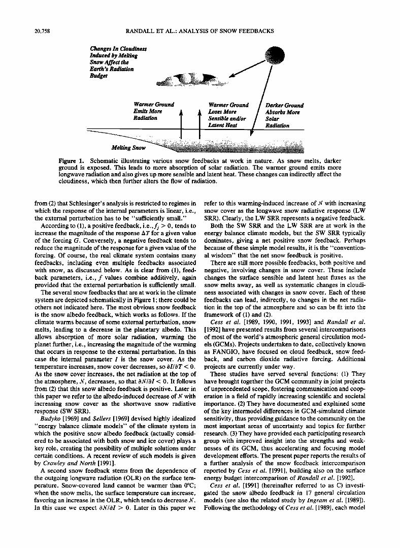
Figure 1. Schematic illustrating various snow feedbacks at work in nature. As snow melts, darker ground is exposed. This leads to more absorption of solar radiation. The warmer ground emits more longwave radiation and also gives up more sensible and latent heat. These changes can indirectly affect the cloudiness, which then further alters the flow of radiation.

from (2) that Schlesinger's analysis is restricted to regimes in which the response of the internal parameters is linear, i.e., the external perturbation has to be "sufficiently small."

According to (1), a positive feedback, i.e., fj > 0, tends to increase the magnitude of the response A T for a given value of the forcing G. Conversely, a negative feedback tends to reduce the magnitude of the response for a given value of the forcing. Of course, the real climate system contains many feedbacks, including even multiple feedbacks associated with snow, as discussed below. As is clear from (1), feedback parameters, i.e., f values combine additively, again provided that the external perturbation is sufficiently small.

The several snow feedbacks that are at work in the climate

system are depicted schematically in Figure 1; there could be others not indicated here. The most obvious snow feedback

is the snow albedo feedback, which works as follows. If the climate warms because of some external perturbation, snow melts, leading to a decrease in the planetary albedo. This allows absorption of more solar radiation, warming the planet further, i.e., increasing the magnitude of the warming that occurs in response to the external perturbation. In this case the internal parameter I is the snow cover. As the temperature increases, snow cover decreases, so 0I/0 T < O. As the snow cover increases, the net radiation at the top of the atmosphere, X, decreases, so that •/•I < 0. It follows from (2) that this snow albedo feedback is positive. Later in this paper we refer to the albedo-induced decrease of X with increasing snow cover as the shortwave snow radiative response (SW SRR).

Budyko [1969] and Sellers [1969] devised highly idealized "energy balance climate models" of the climate system in which the positive snow albedo feedback (actually considered to be associated with both snow and ice cover) plays a key role, creating the possibility of multiple solutions under certain conditions. A recent review of such models is given by Crowley and North [1991].

A second snow feedback stems from the dependence of the outgoing longwave radiation (OLR) on the surface temperature. Snow-covered land cannot be warmer than 0øC; when the snow melts, the surface temperature can increase, favoring an increase in the OLR, which tends to decrease X. In this case we expect •/•I > 0. Later in this paper we

refer to this warming-induced increase of X with increasing snow cover as the longwave snow radiative response (LW SRR). Clearly, the LW SRR represents a negative feedback.

Both the SW SRR and the LW SRR are at work in the

energy balance climate models, but the SW SRR typically dominates, giving a net positive snow feedback. Perhaps because of these simple model results, it is the "conventional wisdom" that the net snow feedback is positive.

There are still more possible feedbacks, both positive and negative, involving changes in snow cover. These include changes the surface sensible and latent heat fluxes as the snow melts away, as well as systematic changes in cloudiness associated with changes in snow cover. Each of these feedbacks can lead, indirectly, to changes in the net radiation in the top of the atmosphere and so can be fit into the framework of (1) and (2).

Cess et al. [1989, 1990, 1991, 1993] and Randall et al. [1992] have presented results from several intercomparisons of most of the world' s atmospheric general circulation models (GCMs). Projects undertaken to date, collectively known as FANGIO, have focused on cloud feedback, snow feedback, and carbon dioxide radiative forcing. Additional projects are currently under way.

These studies have served several functions: (1) They have brought together the GCM community in joint projects of unprecedented scope, fostering communication and coop- eration in a field of rapidly increasing scientific and societal importance. (2) They have documented and explained some of the key intermodel differences in GCM-simulated climate sensitivity, thus providing guidance to the community on the most important areas of uncertainty and topics for further research. (3) They have provided each participating research group with improved insight into the strengths and weak- nesses of its GCM, thus accelerating and focusing model development efforts. The present paper reports the results of a further analysis of the snow feedback intercomparison reported by Cess et al. [1991], building also on the surface energy budget intercomparison of Randall et al. [1992].

Cess et al. [1991] (hereinafter referred to as C) investi- gated the snow albedo feedback in 17 general circulation models (see also the related study by Ingram et al. [1989]). Following the methodology of Cess et al. [1989], each model

RANDALL ET AL.: ANALYSIS OF SNOW FEEDBACKS 20,759

was run with sea surface temperatures (SSTs) artificially increased by 2 K everywhere over the globe, relative to climatology (the "+2 K" runs) and again with SSTs artificially decreased by 2 K everywhere relative to climatology (the "-2 K" runs). Perpetual April simulations were used, since a pilot study indicated that April represents a good compromise between large northern hemisphere snow cover and strong northern hemisphere insolation. Each model was used to perform either one or two -2 K runs (see the discussion of run procedures below) and two +2 K runs. In the first +2 K run the snow cover was allowed to retreat in

response to the prescribed warming of the oceans. In the second +2 K run the snow cover was held fixed at that

obtained in a -2 K run.

For each pair of +2 K and -2 K runs a "climate sensitivity parameter" A was computed from

A = AT/G, (3)

where AT is the change in the globally averaged surface temperature, and G is the change in the net radiation at the top of the atmosphere. Because A measures the change in surface temperature per unit change in the net radiation at the top of the atmosphere, it is a measure of climate sensitivity.

The ratio A/As was interpreted as a measure of the snow feedback; here the subscript s denotes the value of A obtained in a pair of runs (+ 2 K, -2 K) for which the snow cover was fixed. For A/As > 1 the climate sensitivity with variable snow is greater than that with fixed snow, so we can say that changes in snow cover have increased the climate sensitivity. In this sense, A/As is a measure of the snow feedback.

The main conclusions of C were as follows.

1. The snow feedback is negative in some models and positive in others. Only weak negative feedbacks were obtained by a few models, however, while most models produced positive snow feedbacks, some of them fairly strong.

2. The direct snow albedo feedback is only a portion of the total snow feedback. Numerous indirect snow feedbacks

occur, involving changes in the surface temperature and cloudiness. The magnitudes of the various direct and indirect snow feedbacks differ significantly from one model to another.

C's overall conclusion was that even the apparently straightforward snow feedback is difficult to characterize without careful, quantitative consideration of the full com- plexity of the climate system.

A full analysis of the results of C's snow feedback intercomparison obviously has to entail an investigation of the surface energy budgets of the models and how they changed when the SSTs were perturbed. A surface energy budget intercomparison has already been carried out for the July runs. Randall et al. [1992] analyzed the surface energy budgets of 19 GCMs, and their responses to SST perturbations of +2 K and -2 K SST, in the perpetual July simulations (see also D•qu• and Royer [1991]). Randall et al. identified major differences in the responses of the various components of the surface energy flux to the imposed 4 K warming. They showed that these differences were largely associated with the simulated hydrologic cycles and the parameterizations of longwave radiation and cumulus con- vection.

The present study applies the methodology of Randall et al. [1992] to snow feedback experiments that are essentially the same as those of C. The purpose of this study is to investigate, in more detail, how and why negative or weak positive snow feedbacks occurred in some of the models, while others produced strong positive snow feedbacks. Our approach is to focus on the changes in the simulated surface energy budgets and their role in snow feedback.

Although we show some results from 14 GCMs, we focus particular attention on two of the models, those of Colorado State University (CSU) and the Australian Bureau of Mete- orological Research Centre (BMRC). A detailed analysis of the snow feedback experiments performed with the BMRC model has already been published by Colman et al. [1993]. Detailed analyses of the results from other individual models may be published in the future by the various research groups involved.

It is important to emphasize that neither C's study nor the present study is intended to determine the magnitude of the snow feedback that would occur in a possible climate change scenario such as that which might result from increasing greenhouse gas concentrations. The numerical experiments involved are deliberately idealized. As explained below, many gross simplifying assumptions have been made, for example, perpetual April conditions and drastically and uniformly increased SSTs without corresponding changes in sea ice distributions. These idealizations make it impossible to interpret the results in terms of realistic climate change, but at the same time they make the numerical experiments simple enough and economical enough so that a diverse group of investigators, scattered around the world, with differing levels of computational and human resources, have been able to work together on a joint calculation. The results of this calculation, while not directly applicable to the climate prediction problems facing the world today, have nevertheless been educational in the sense that they have surprised us with outcomes that we did not anticipate and in so doing have taught us something about the physics of climate change.

2. Description of Models and Simulations 2.1. Models

The participating models are listed in Table 1. A few of the models that participated in the snow albedo study of C and the surface energy budget study of Randall et al. [ 1992] were not available for the present study. References giving detailed descriptions of the models were listed by Cess et al. [1989, 1990, 1991].

All of the models include the mass of snow on the ground as a prognostic variable. If the temperature of the lowest atmospheric level is below fleezing, then any precipitation that occurs is assumed to fall as snow, although the BMRC, European Centre for Medium-Range Weather Forecasts (ECMWF), and ECHAM models depart slightly from this nominal procedure. The snow mass budget of each model takes into account snowfall, melting, and sublimation, although the methods used to do so vary considerably from model to model.

The snow albedo is parameterized quite differently among the models. It can be a function of one or more the following quantities: snow depth, age, and temperature. In addition, the snow albedo is, in some models, substantially reduced


Table 1. A List of the Participating GCMs and the Experimental Design Used by Each

Model Model Number

Same Results as Length of Run, Reported by Cess et al. Run days/Averaging

[ 1991].9 Procedure Interval, days Ground Wetness

Initialization

BMRC 12 CCC 6 CCM/LLNL 13

CNRM 8 CSU 1

ECMWF 3

ECHAM 7 GFDL 2 GISS 5 OSU/IAP 14 IAP/SUNY 4

LMD 11 MGO 10

MRI 9

yes B 210/90 yes B 100/30 same runs, but different A 340/270

averaging period no B 100/30

yes B 180/120

yes A 90/30

yes B 120/90 yes B 180/90 yes B 360/210 yes B 120/30 no; new runs with a B 106/30

revised model no B 60/30

same runs, but different B 120/90 averaging period

yes B 90/30

Mintz and $erafini [1983] previous long seasonal run previous long seasonal run

previous long seasonal run fixed, based on previous

long seasonal run observed initial condition

supplied by ECMWF previous long seasonal run previous long seasonal run previous long seasonal run previous long seasonal run previous long seasonal run

previous long seasonal run Mintz and $erafini [1983]

Mintz and $erafini [1983]

The model number increases monotonically with the value of A/As, as explained in the text. The run procedure is also explained in the text, with reference to Figure 2. Column 5 shows the lengths of the runs made and also the lengths of the averaging intervals, at the end of each run, over which results were computed.

for forested regions. For the community circulation model (CCM)/Lawrence Livermore National Laboratory (LLNL) only half of any snow-covered grid area is assigned the albedo of snow; the other half retains the bare ground albedo.

In all of the models the emissivity of the snow is assumed to be unity, for simplicity.

2.2. Experiment Design

The initial conditions used were in all cases taken from

earlier, long, seasonally varying simulations with the respective models.

As discussed in section 1, the basic idea of our experiment is this: We conducted two pairs of simulations with each model. In the first pair of runs, called the "variable-snow" runs, snow cover was allowed to vary according to each model's formulation. The sea surface temperatures were instantaneously perturbed from their observed climatological April distributions by a globally uniform + 2 K and -2 K in the respective runs. The distribution of sea ice was unchanged, for simplicity. We might naively expect that snow will melt in the "warm" variable-snow run, relative to the "cold" variable-snow run, and that this removal of the snow in the warm run will lead to the absorption of more solar radiation at the Earth's surface, thus reinforcing the warming through the snow albedo feedback. This would of course be a positive snow feedback, because the initial imposed warming would be reinforced by the response of the snow. In the present context, with imposed SST changes and computed top-of-the-atmosphere radiation changes, a positive snow feedback manifests itself as an increased climate

sensitivity parameter. The second pair of simulations is just like the first, except

that the snow at each grid point is held fixed at the value obtained in the cold variable-snow run. We refer to this pair of runs as the "fixed-snow" runs. Because the snow cover is

fixed at the values obtained in the cold variable-snow run,

the snow cannot melt in response to the imposed sea surface temperature increase, and so the snow feedback cannot operate.

The effects of artificially fixing the snow cover are somewhat complex. Most obviously, the surface albedo remains high, relative to that of snow-free ground. A second effect is that the surface temperature at a snow-covered point cannot exceed 0øC, although in some of the models this was permitted to occur in the fixed-snow runs. To the extent that the surface temperature at fixed-snow points is lower than it otherwise would have been, the surface longwave radiation, sensible heat flux, and evaporation will all be affected. Note also that the snow albedo may depend on the predicted temperature of the fixed snow; this point is discussed further later. A third effect of fixing the snow cover is that a snow surface is wet, promoting evaporation that otherwise might not have occurred.

By comparing the climate sensitivity parameter between the variable-snow runs and the fixed-snow runs, we can determine the magnitude of the snow feedback.

Although it was our collective intention that a single experimental design be executed with all of the GCMs, we discovered after the fact that because of differences of

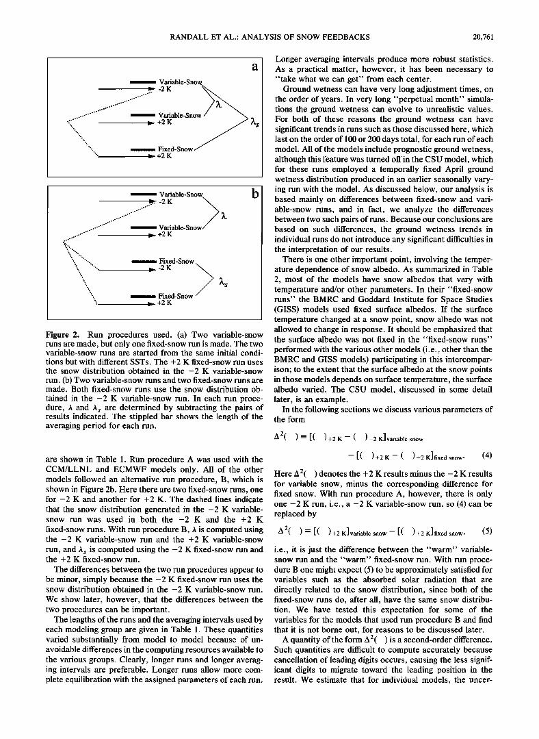
interpretation, the experiments performed with the various GCMs followed one of two generally similar procedures. In run procedure A, shown in Figure 2a, the lines with arrow- heads represent runs, and the stippled bars indicate averaging intervals. The dashed line indicates that the snow produced in the -2 K variable-snow run was used in the + 2 K

fixed-snow run. Note that in run procedure A, there is no -2 K fixed-snow run. The two variable-snow runs are of course

directly comparable, and we expect to find less snow in the + 2 K run. With run procedure A, A is computed using the -2 K variable-snow run and the + 2 K variable-snow run, and As is computed using the -2 K variable-snow run and the + 2 K fixed-snow run.

The run procedures actually used with the various GCMs

RANDALL ET AL ß ANALYSIS OF SNOW FEEDBACKS 20,761

.............. • Variable-Sno

'"'"'"".. '"' ------------ Fixed-Snow '5... '"., - ......................... +2

Variable-Snow.

-2 K • Variable-Snow +2K

.•:.•_..• Fixed-Snow

• -2 K • •'s :• Fixed_Snow •-• +2 K

b

Figure 2. Run procedures used. (a) Two variable-snow runs are made, but only one fixed-snow run is made. The two variable-snow runs are started from the same initial conditions but with different SSTs. The + 2 K fixed-snow run uses the snow distribution obtained in the -2 K variable-snow

run. (b) Two variable-snow runs and two fixed-snow runs are made. Both fixed-snow runs use the snow distribution ob-

tained in the -2 K variable-snow run. In each run procedure, A and As are determined by subtracting the pairs of results indicated. The stippled bar shows the length of the averaging period for each run.

Longer averaging intervals produce more robust statistics. As a practical matter, however, it has been necessary to "take what we can get" from each center.

Ground wetness can have very long adjustment times, on the order of years. In very long "perpetual month" simulations the ground wetness can evolve to unrealistic values. For both of these reasons the ground wetness can have significant trends in runs such as those discussed here, which last on the order of 100 or 200 days total, for each run of each model. All of the models include prognostic ground wetness, although this feature was turned off in the CSU model, which for these runs employed a temporally fixed April ground wetness distribution produced in an earlier seasonally varying run with the model. As discussed below, our analysis is based mainly on differences between fixed-snow and variable-snow runs, and in fact, we analyze the differences between two such pairs of runs. Because our conclusions are based on such differences, the ground wetness trends in individual runs do not introduce any significant difficulties in the interpretation of our results.

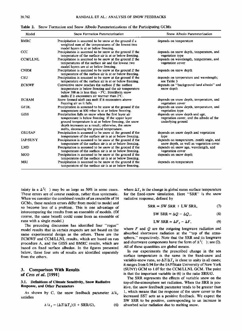
There is one other important point, involving the temperature dependence of snow albedo. As summarized in Table 2, most of the models have snow albedos that vary with temperature and/or other parameters. In their "fixed-snow runs" the BMRC and Goddard Institute for Space Studies (GISS) models used fixed surface albedos. If the surface temperature changed at a snow point, snow albedo was not allowed to change in response. It should be emphasized that the surface albedo was not fixed in the "fixed-snow runs"

performed with the various other models (i.e., other than the BMRC and GISS models) participating in this intercomparison; to the extent that the surface albedo at the snow points in those models depends on surface temperature, the surface albedo varied. The CSU model, discussed in some detail later, is an example.

In the following sections we discuss various parameters of the form

A 2( ) • [( ) +2 K -- ( )-2 K]variable snow

are shown in Table 1. Run procedure A was used with the CCM/LLNL and ECMWF models only. All of the other models followed an alternative run procedure, B, which is shown in Figure 2b. Here there are two fixed-snow runs, one for -2 K and another for +2 K. The dashed lines indicate

that the snow distribution generated in the -2 K variable- snow run was used in both the -2 K and the +2 K

fixed-snow runs. With run procedure B, A is computed using the -2 K variable-snow run and the +2 K variable-snow

run, and A s is computed using the -2 K fixed-snow run and the +2 K fixed-snow run.

The differences between the two run procedures appear to be minor, simply because the -2 K fixed-snow run uses the snow distribution obtained in the -2 K variable-snow run.

We show later, however, that the differences between the two procedures can be important.

The lengths of the runs and the averaging intervals used by each modeling group are given in Table 1. These quantities varied substantially from model to model because of un- avoidable differences in the computing resources available to the various groups. Clearly, longer runs and longer averaging intervals are preferable. Longer runs allow more com- plete equilibration with the assigned parameters of each run.

-- [ ( ) +2 K -- ( ) -2 K] fixed snow' (4)

Here A2( ) denotes the +2 K results minus the -2 K results for variable snow, minus the corresponding difference for fixed snow. With run procedure A, however, there is only one -2 K run, i.e., a -2 K variable-snow run, so (4) can be replaced by

A 2( ) = [( ) +2 K]variable snow -- [( ) +2 K]fixed snow, (5)

i.e., it is just the difference between the "warm" variable- snow run and the "warm" fixed-snow run. With run procedure B one might expect (5) to be approximately satisfied for variables such as the absorbed solar radiation that are

directly related to the snow distribution, since both of the fixed-snow runs do, after all, have the same snow distribution. We have tested this expectation for some of the variables for the models that used run procedure B and find that it is not borne out, for reasons to be discussed later.

A quantity of the form A2( ) is a second-order difference. Such quantities are difficult to compute accurately because cancellation of leading digits occurs, causing the less significant digits to migrate toward the leading position in the result. We estimate that for individual models, the uncer-


Table 2. Snow Formation and Snow Albedo Parameterizations of the Participating GCMs

Model Snow Formation Parameterization Snow Albedo Parameterization

BMRC Precipitation is assumed to be snow at the ground if a depends on temperature

CCC

CCM/LLNL

CNRM

csu

ECMWF

ECHAM

GFDL

GISS

OSU/IAP

IAP/SUNY

LMD

MGO

MRI

weighted sum of the temperatures of the lowest two model layers is at or below freezing.

Precipitation is assumed to be snow at the ground if the temperature of the surface air is at or below freezing.

Precipitation is assumed to be snow at the ground if the temperatures of the surface air and the lowest two model layers are at or below freezing.



Convective snow reaches the surface if the surface

temperature is below freezing and the air temperature below 300 m is less than -3øC. Stratiform snow melts if it encounters air warmer than 2øC.

Snow formed aloft can melt if it encounters above-

freezing air as it falls. Precipitation is assumed to be snow at the ground if the

temperature at 850 mbar is at or below freezing. Precipitation falls as snow when the first layer air

temperature is below freezing. If the upper layer ground temperature is at or below freezing, the snow depth increases as a result; otherwise, the snow melts, decreasing the ground temperature.






depends on snow depth, temperature, and vegetation type

depends on wavelength, temperature, and vegetation cover

depends on snow depth

depends on temperature and wavelength; see Table 3

depends on "background land albedo" and snow depth

depends on snow depth, temperature, and vegetation cover

depends on snow depth, temperature, and vegetation type

depends on snow depth and age, vegetation cover, and the albedo of the underlying ground

depends on snow depth and vegetation type

depends on temperature, zenith angle, and snow depth, as well as vegetation cover

depends on snow age, wavelength, and vegetation cover

depends on snow depth

depends on temperature

tainty in a A2( ) may be as large as 50% in some cases. These errors are of course random, rather than systematic. When we consider the combined results of an ensemble of 14

GCMs, these random errors differ from model to model and so become less of a problem. This is one advantage of intercomparing the results from an ensemble of models. (Of course, the same benefit could come from an ensemble of runs with a single model.)

The preceding discussion has identified four "rogue" model results that in certain respects are not based on the same experimental design as the others. These are the ECMWF and CCM/LLNL results, which are based on run procedure A, and the GISS and BMRC results, which are based on fixed surface albedos. In the figures presented below, these four sets of results are identified separately from the others.

3. Comparison With Results of Cess et al. [1991]

3.1. Definitions of Climate Sensitivity, Snow Radiative Response, and Other Parameters

As shown by C, the snow feedback parameter A/As satisfies

AIA s = (AT/ATs) (1 + SRR/G), (6)

where ATs is the change in global mean surface temperature for the fixed-snow simulation. Here "SRR" is the snow

radiative response, defined by

SRR -- SW SRR + LW SRR, (7)

SW SRR--AQ- AQs , (8)

LW SRR = AF s - AF, (9)

where F and Q are the outgoing longwave radiation and absorbed shortwave radiation at the "top of the atmosphere," respectively. Note that the SRR and its longwave and shortwave components have the form of A2( ); see (2). All of these quantities are global means.

In our experiments the prescribed change in the sea surface temperature is the same in the fixed-snow and variable-snow runs, so AT/ATs is close to unity in all cases; it ranges from 0.94 for the IAP/State University of New York (SUNY) GCM to 1.07 for the CCM/LLNL GCM. The point is that the important variable in (6) is the ratio SRR/G.

The SRR represents the effects of variable snow on the top-of-the-atmosphere net radiation. When the SRR is positive, the snow feedback parameter tends to be greater than 1, which means that the response of the snow cover to the increased SST acts as a positive feedback. We expect the SW SRR to be positive, corresponding to an increase in absorbed solar radiation due to melting snow.

RANDALL ET AL.' ANALYSIS OF SNOW FEEDBACKS 20,763

The total SRR/G ranges from -0.117 for the Geophysical Fluid Dynamics Laboratory (GFDL) GCM, which has a negative snow feedback, to 0.195 for the BMRC GCM, which has a strong positive snow feedback. In section 4 we compare the results obtained with these two models directly and in some detail.

3.2. Analysis in the Spirit of C

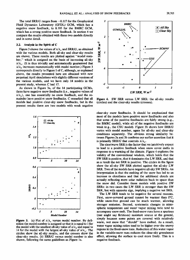
Figure 3 shows the values of A/As and SRR/G, as obtained with the various models. Both all-sky and clear-sky results are shown. These results are plotted against "model number," which is assigned on the basis of increasing all-sky A/As. (It is thus trivially and automatically guaranteed that A/As increases monotonically with model number.) Figure 3 corresponds directly to Figure 1 of C, although, as explained above, the results presented here are obtained with new perpetual April simulations with slightly different versions of the various models, and we have only 14 models in the present study, whereas C had 17.

As shown in Figure 3a, of the 14 participating GCMs, three have negative snow feedbacks (i.e., negative values of A/As), one has essentially no snow feedback, and the re- mainder have positive snow feedbacks. C remarked that all models had positive clear-sky snow feedbacks, but in the present results there are two models with weak negative

BMRC

CCM/LLNL ••

xO

ß x x

ß

ß x

All Sky Clear Sky

ß

< x - -- ECMWF x

-2 -1 0 1 2

LW SRR, W m '2

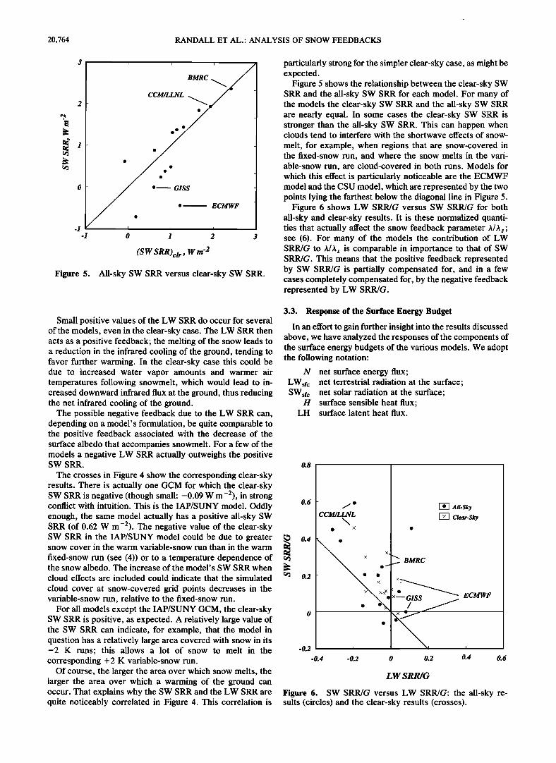
Figure 4. SW SRR versus LW SRR: the all-sky results (circles) and the clear-sky results (crosses).

1.6

1.4

1.0

0.8

All. S• Clear. Sky

x

x

x ß

x ß ß

• x ß ß ß x

• ß x

0.6

0.4

0.2

-0.2

x

ß x ß ß ß

ß • • x x x

x

x

ß

x x ß ß

i i f i i i i i i i i i i i

1 5 10 14

Model Number

Figure 3. (a) Plot of A/As versus model number. By definition the model number is assigned so that it is equal to 1 for the model with the smallest all-sky value of A/A s and equal to 14 for the model with the largest all-sky value of A/As. The circles show the all-sky results, and the crosses show the clear-sky results. (b) SRR/G versus model number is also shown, following the same guidelines as Figure la.

clear-sky snow feedbacks. It should be emphasized that most of the models have positive snow feedbacks and also that some of the positive feedbacks are fairly strong (e.g., the B MRC model), while all of the negative feedbacks are weak (e.g., the CSU model). Figure 3b shows how SRR/G varies with model number, again for all-sky and clear-sky conditions separately. The obvious strong similarity between Figures 3a and 3b confirms our earlier assertion that it is primarily SRR/G that controls A/As.

The shortwave SRR is the factor that we intuitively expect to lead to a positive feedback when snow cover melts in response to a warming of the climate. Figure 4 explores the validity of the conventional wisdom, which holds that the SW SRR is positive, that it dominates the LW SRR, and that as a result the net SRR is positive. The circles in the figure show the all-sky SW SRR plotted against the all-sky LW SRR. Two of the models have negative all-sky SW SRRs. An interpretation is that the melting of the snow has led to an increase in cloudiness and that the additional clouds are

actually reflecting more solar radiation back to space than the snow did. Consider those models with positive SW SRRs: in two cases the LW SRR is stronger than the SW SRR, but with opposite sign, implying a negative net SRR.

The LW SRR tends to be negative for several reasons. First, snow-covered ground cannot be warmer than 0øC, while snow-free ground can be much warmer, allowing stronger emission. Second, systematic changes in atmospheric temperature and water vapor mixing ratio tend to accompany snow melt. The fixed-snow runs have a spurious (one might say fictitious) moisture source at the ground, simply because some points are covered with relatively warm, wet snow that "should" have melted. As a result, water vapor mixing ratios tend to be higher over the snowy regions in the fixed-snow runs. Reduction of this water vapor in the variable-snow runs reduces the clear-sky greenhouse effect, allowing the surface to cool more freely. This is a negative feedback.

20,764 RANDALL ET AL.' ANALYSIS OF SNOW FEEDBACKS

2

-1 -1

, , , j

CCM/LLNL •

•----- GISS - ß •------- ECMWF

0 1 2 3

(SW SRR)clr , W m '2

Figure 5. All-sky SW SRR versus clear-sky SW SRR.

particularly strong for the simpler clear-sky case, as might be expected.

Figure 5 shows the relationship between the clear-sky SW SRR and the all-sky SW SRR for each model. For many of the models the clear-sky SW SRR and the all-sky SW SRR are nearly equal. In some cases the clear-sky SW SRR is stronger than the all-sky SW SRR. This can happen when clouds tend to interfere with the shortwave effects of snow-

melt, for example, when regions that are snow-covered in the fixed-snow run, and where the snow melts in the variable-snow run, are cloud-covered in both runs. Models for which this effect is particularly noticeable are the ECMWF model and the CSU model, which are represented by the two points lying the farthest below the diagonal line in Figure 5.

Figure 6 shows LW SRR/G versus SW SRR/G for both all-sky and clear-sky results. It is these normalized quantities that actually affect the snow feedback parameter A/As; see (6). For many of the models the contribution of LW SRR/G to A/As is comparable in importance to that of SW SRR/G. This means that the positive feedback represented by SW SRR/G is partially compensated for, and in a few cases completely compensated for, by the negative feedback represented by LW SRR/G.

Small positive values of the LW SRR do occur for several of the models, even in the clear-sky case. The LW SRR then acts as a positive feedback; the melting of the snow leads to a reduction in the infrared cooling of the ground, tending to favor further warming. In the clear-sky case this could be due to increased water vapor amounts and warmer air temperatures following snowmelt, which would lead to increased downward infrared flux at the ground, thus reducing the net infrared cooling of the ground.

The possible negative feedback due to the LW SRR can, depending on a model's formulation, be quite comparable to the positive feedback associated with the decrease of the surface albedo that accompanies snowmelt. For a few of the models a negative LW SRR actually outweighs the positive SW SRR.

The crosses in Figure 4 show the corresponding clear-sky results. There is actually one GCM for which the clear-sky SW SRR is negative (though small: -0.09 W m-2), in strong conflict with intuition. This is the IAP/SUNY model. Oddly enough, the same model actually has a positive all-sky SW SRR (of 0.62 W m-2). The negative value of the clear-sky SW SRR in the IAP/SUNY model could be due to greater snow cover in the warm variable-snow run than in the warm

fixed-snow run (see (4)) or to a temperature dependence of the snow albedo. The increase of the model's SW SRR when

cloud effects are included could indicate that the simulated

cloud cover at snow-covered grid points decreases in the variable-snow run, relative to the fixed-snow run.

For all models except the IAP/SUNY GCM, the clear-sky SW SRR is positive, as expected. A relatively large value of the SW SRR can indicate, for example, that the model in question has a relatively large area covered with snow in its -2 K runs; this allows a lot of snow to melt in the corresponding +2 K variable-snow run.

Of course, the larger the area over which snow melts, the larger the area over which a warming of the ground can occur. That explains why the SW SRR and the LW SRR are quite noticeably correlated in Figure 4. This correlation is

3.3. Response of the Surface Energy Budget

In an effort to gain further insight into the results discussed above, we have analyzed the responses of the components of the surface energy budgets of the various models. We adopt the following notation:

N net surface energy flux; LWsfc net terrestrial radiation at the surface; SWsfc net solar radiation at the surface;

H surface sensible heat flux; LH surface latent heat flux.

0.8

0.6

0.4

0.2

-0.2

-0.4 0.6

• ß • All-Sky CCM/LLNL •7• Clear. Sky

ß x ß

• BMRC

xxX I < • •l • GISS • EC•F

. ./

-0.2 0 0.2 0.4

LW SRR/G

Figure 6. SW SRR/G versus LW SRR/G: the all-sky results (circles) and the clear-sky results (crosses).

RANDALL ET AL' ANALYSIS OF SNOW FEEDBACKS 20,765

• • Variable Snow • Fixed Snow

•GISS '7 l CCM/LLNL• x x

- •,

ECMWF 'x• ß - I I t I i•øl•

.lO

.12 -2 0 2 4 6 8 10 12

G, Wm

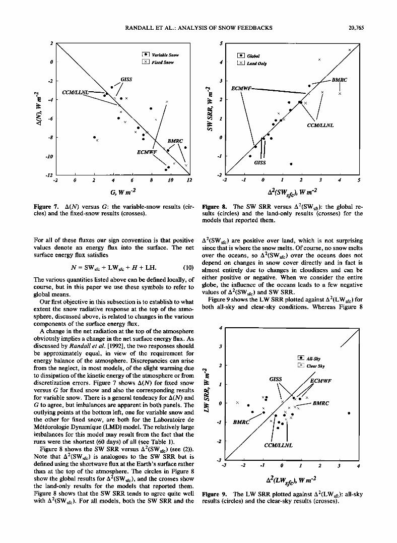
Figure 7. A(N) versus G' the variable-snow results (circles) and the fixed-snow results (crosses).

• Global

4 [-• Land Only x

3 •.-BMRC • ECMWF I

• • x/ x x

• ,

..1'

GISS ß -2 -1 0 1 2 3 4 5

a(SWsfc), W m Figure 8. The SW SRR versus A2(SWsft) ß the global results (circles) and the land-only results (crosses) for the models that reported them.

For all of these fluxes our sign convention is that positive values denote an energy flux into the surface. The net surface energy flux satisfies

N = SWsfc + LWsfc + H + LH. (10)

The various quantities listed above can be defined locally, of course, but in this paper we use these symbols to refer to global means.

Our first objective in this subsection is to establish to what extent the snow radiative response at the top of the atmosphere, discussed above, is related to changes in the various components of the surface energy flux.

A change in the net radiation at the top of the atmosphere obviously implies a change in the net surface energy flux. As discussed by Randall et al. [1992], the two responses should be approximately equal, in view of the requirement for energy balance of the atmosphere. Discrepancies can arise from the neglect, in most models, of the slight warming due to dissipation of the kinetic energy of the atmosphere or from discretization errors. Figure 7 shows A(N) for fixed snow versus G for fixed snow and also the corresponding results for variable snow. There is a general tendency for A(N) and G to agree, but imbalances are apparent in both panels. The outlying points at the bottom left, one for variable snow and the other for fixed snow, are both for the Laboratoire de M6t6orologie Dynamique (LMD) model. The relatively large imbalances for this model may result from the fact that the runs were the shortest (60 days) of all (see Table 1).

Figure 8 shows the SW SRR versus A2(SWsfc) (see (2)). Note that A2(SWsfc) is analogous to the SW SRR but is defined using the shortwave flux at the Earth' s surface rather than at the top of the atmosphere. The circles in Figure 8 show the global results for A2(SWsfc), and the crosses show the land-only results for the models that reported them. Figure 8 shows that the SW SRR tends to agree quite well with A2(SWsfc). For all models, both the SW SRR and the

A2(SWsfc) are positive over land, which is not surprising since that is where the snow melts. Of course, no snow melts over the oceans, so A2(SWsfc) over the oceans does not depend on changes in snow cover directly and in fact is almost entirely due to changes in cloudiness and can be either positive or negative. When we consider the entire globe, the influence of the oceans leads to a few negative values of A2(SWsfc) and SW SRR.

Figure 9 shows the LW SRR plotted against A2(LWsfc) for both all-sky and clear-sky conditions. Whereas Figure 8

All-Sky Clear Sky

-3 I

-3 3 4

ass

/• •CCM/LLNL • -2 -1 0 1 2

A2(LWsfc), W m '2 Figure 9. The LW SRR plotted against A2(LWsft) ß all-sky results (circles) and the clear-sky results (crosses).


m

_

_

_

..2 -÷

-4-

-6'

A 2 of the Surface Fluxes I

LH H

I '

BMRC CCC CCM/ CNRM CSU ECHAM ECMWF GFDL GISS IAP/ IAP/ LMD MGO LLNL OSU SUNY

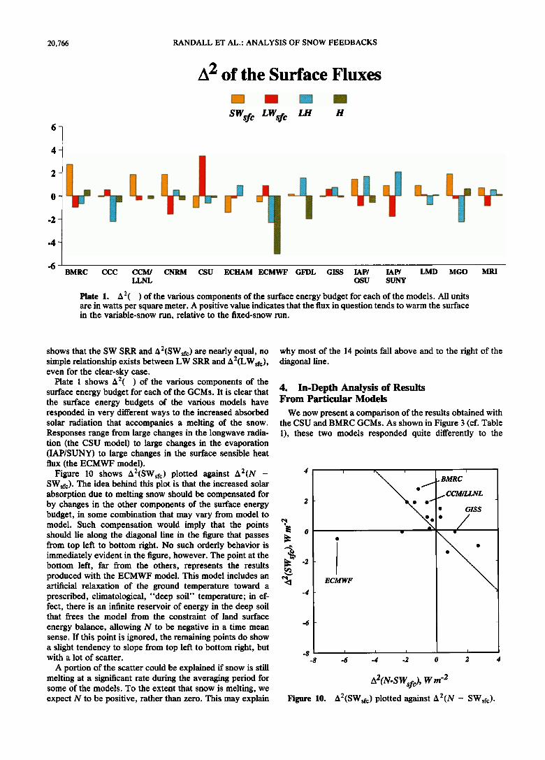
Plate 1. A2( ) of the various components of the surface energy budget for each of the models. All units are in watts per square meter. A positive value indicates that the flux in question tends to warm the surface in the variable-snow run, relative to the fixed-snow run.

MRI

shows that the SW SRR and A2(SWsfc) are nearly equal, no simple relationship exists between LW SRR and A2(LWsfc), even for the clear-sky case.

Plate I shows A2( ) of the various components of the surface energy budget for each of the GCMs. It is clear that the surface energy budgets of the various models have responded in very different ways to the increased absorbed solar radiation that accompanies a melting of the snow. Responses range from large changes in the longwave radiation (the CSU model) to large changes in the evaporation (IAP/SUNY) to large changes in the surface sensible heat flux (the ECMWF model).

Figure 10 shows A2(SWsfc) plotted against A2(N - SWsfc). The idea behind this plot is that the increased solar absorption due to melting snow should be compensated for by changes in the other components of the surface energy budget, in some combination that may vary from model to model. Such compensation would imply that the points should lie along the diagonal line in the figure that passes from top left to bottom right. No such orderly behavior is immediately evident in the figure, however. The point at the bottom left, far from the others, represents the results produced with the ECMWF model. This model includes an artificial relaxation of the ground temperature toward a prescribed, climatological, "deep soil" temperature; in effect, there is an infinite reservoir of energy in the deep soil that frees the model from the constraint of land surface

energy balance, allowing N to be negative in a time mean sense. If this point is ignored, the remaining points do show a slight tendency to slope from top left to bottom right, but with a lot of scatter.

A portion of the scatter could be explained if snow is still melting at a significant rate during the averaging period for some of the models. To the extent that snow is melting, we expect N to be positive, rather than zero. This may explain

why most of the 14 points fall above and to the right of the diagonal line.

4. In-Depth Analysis of Results From Particular Models

We now present a comparison of the results obtained with the CSU and BMRC GCMs. As shown in Figure 3 (cf. Table 1), these two models responded quite differently to the

-6

-8 -8

ß • •. BMRC j CCM/LLNL

ß GISS

/

ECMWF

_

_

-6 -4 -2 0 2 4

Figure 10.

A2(N-SWsfc ), W m '2 A2(SWsfc) plotted against A2(N - SWsfc).


imposed sea surface temperature increase. The CSU model produced a weak negative snow feedback, while the BMRC model gave a strong positive snow feedback.

4.1. BMRC

Colman et al. [1993] have reported a detailed analysis of the strong positive snow feedback that occurs in the BMRC GCM. Their study is based directly on the FANGIO simulations used in the present paper. Here we briefly summarize their results.

For both snow and sea ice points the albedo a is prescribed to increase as the surface temperature drops as follows:

(T- 263.1 K) =0.7- (0.7-0.4) (11)

10K

263.1 K-<T-<273.1 K.

For temperatures less than 263.1 K the albedo is kept fixed at 0.7. The temperature of a snow-covered point cannot exceed 273.1 K. The albedo of snow-free land is specified following Hummel and Reck [ 1979]. If a snow-covered point becomes snow-free during a particular time step, its albedo is reset to the Hummel-Reck value if the point in question was snow-free in the Hummel-Reck climatology. If the point in question was snow-covered in the Hummel-Reck climatology, its albedo is set to 0.12 for simplicity, and in the variable-snow simulations discussed in this paper, that value was retained until the point became covered with snow once more.

As mentioned earlier, in their fixed-snow runs, Colman et al. [1993] held the surface albedo fixed. If the surface temperature changed at a snow point, the temperature dependence shown in (9) was not allowed to affect the albedo. As already discussed (see Table 1 and Figure 3), the BMRC model produced a strong positive snow feedback. The shortwave SRR was 2.40 W m -2, and the longwave SRR was -0.48 W m -2.

Colman et al. [1993, p. 261] give an extensive discussion of the effects of clouds on the snow feedback in their model; this will not be repeated here. They note that the surface albedo drops in the variable-albedo (i.e., variable-snow) experiment, and they conclude that "the difference in response [to the imposed SST increase, between the fixed- albedo and the variable-albedo cases] is determined princi- pally by the change in SW reflected, caused by the albedo changes, but... this response is amplified 100% by... cloud changes."

4.2. CSU

We now analyze the results from the CSU GCM, in order to understand why that model gave a negative snow feedback.

Table 3. Dependence of Snow Albedo on Temperature and Wavelength in the CSU GCM

Visible Near Infrared

Cold snow 0.80 0.40 Warm snow 0.48 0.24

In the model the dividing line between "visible" and "near- infrared" radiation is 0.7 /am. The dividing line between "cold snow" and "warm snow" is -0.05øC.

5O Total Snow Area

$000

0 30 60 90

Total Snow Mass

4ooo

3000

2000

lOOO

+2 K Variable Snow

............ 2 K Variable Snow

0 30 60 90

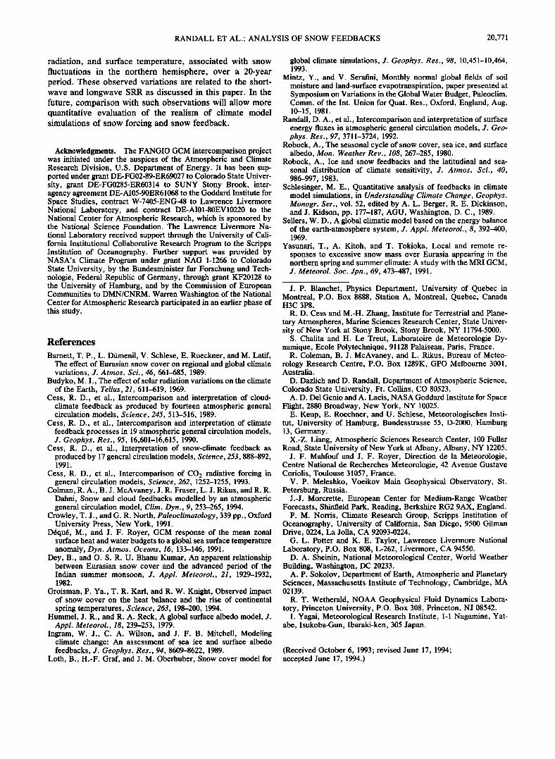
Days

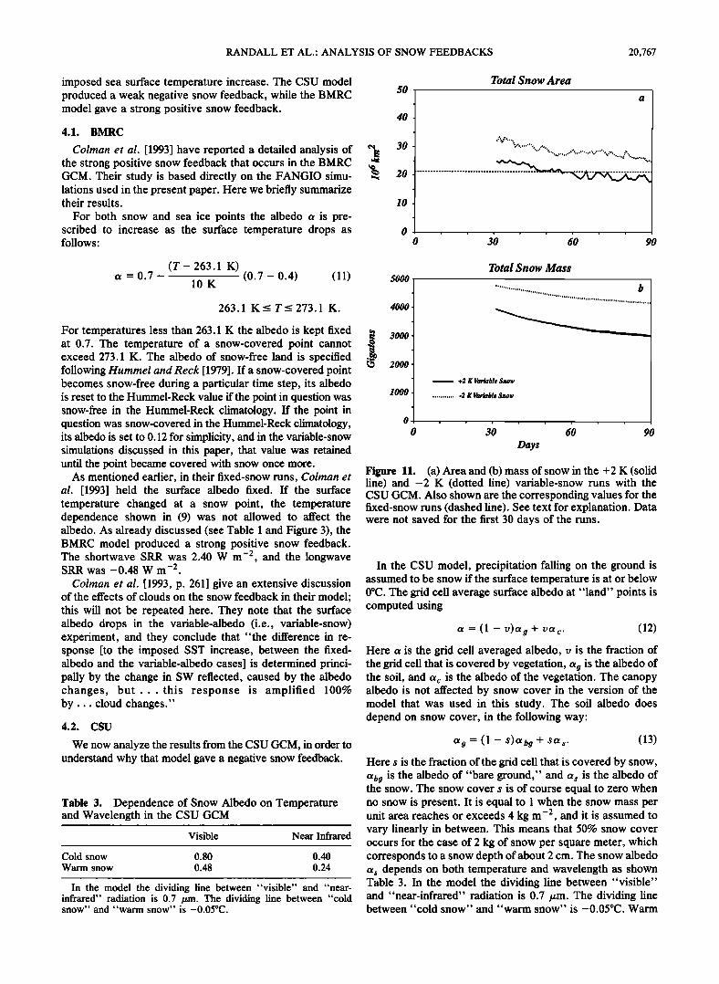
Figure 11. (a) Area and (b) mass of snow in the +2 K (solid line) and -2 K (dotted line) variable-snow runs with the CSU GCM. Also shown are the corresponding values for the fixed-snow runs (dashed line). See text for explanation. Data were not saved for the first 30 days of the runs.

In the CSU model, precipitation falling on the ground is assumed to be snow if the surface temperature is at or below 0øC. The grid cell average surface albedo at "land" points is computed using

a = (1 - v)ag + va c. (12)

Here a is the grid cell averaged albedo, v is the fraction of the grid cell that is covered by vegetation, ag is the albedo of the soil, and a c is the albedo of the vegetation. The canopy albedo is not affected by snow cover in the version of the model that was used in this study. The soil albedo does depend on snow cover, in the following way:

ag = (1 - s)abg + Sas. (13)

Here s is the fraction of the grid cell that is covered by snow, abg is the albedo of "bare ground," and as is the albedo of the snow. The snow cover s is of course equal to zero when no snow is present. It is equal to 1 when the snow mass per unit area reaches or exceeds 4 kg m -2, and it is assumed to vary linearly in between. This means that 50% snow cover occurs for the case of 2 kg of snow per square meter, which corresponds to a snow depth of about 2 cm. The snow albedo as depends on both temperature and wavelength as shown Table 3. In the model the dividing line between "visible" and "near-infrared" radiation is 0.7 /am. The dividing line between "cold snow" and "warm snow" is -0.05øC. Warm


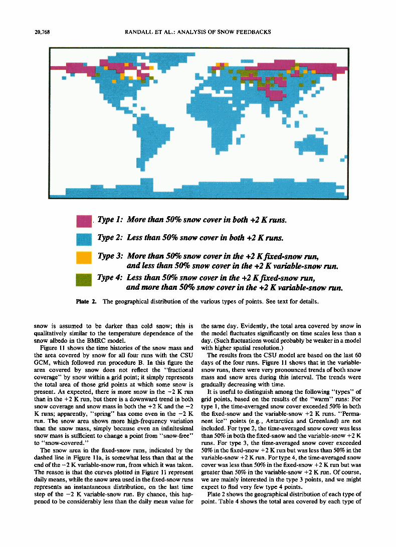
Type 1: More than 50% snow cover in both +2 K runs.

Type 2: Less than 50% snow cover in both +2 K runs.

Type 3: More than $0% snow cover in the +2 K fixed-snow run, and less than 50% snow cover in the +2 K variable-snow run.

Type 4: Less than 50% snow cover in the +2 K fixed-snow run, and more than 50% snow cover in the +2 K variable-snow run.

Plate 2. The geographical distribution of the various types of points. See text for details.

snow is assumed to be darker than cold snow; this is qualitatively similar to the temperature dependence of the snow albedo in the BMRC model.

Figure 11 shows the time histories of the snow mass and the area covered by snow for all four runs with the CSU GCM, which followed run procedure B. In this figure the area covered by snow does not reflect the "fractional coverage" by snow within a grid point; it simply represents the total area of those grid points at which some snow is present. As expected, there is more snow in the -2 K run than in the + 2 K run, but there is a downward trend in both snow coverage and snow mass in both the + 2 K and the -2 K runs; apparently, "spring" has come even in the -2 K run. The snow area shows more high-frequency variation than the snow mass, simply because even an infinitesimal snow mass is sufficient to change a point from "snow-free" to "snow-covered."

The snow area in the fixed-snow runs, indicated by the dashed line in Figure 1 l a, is somewhat less than that at the end of the -2 K variable-snow run, from which it was taken. The reason is that the curves plotted in Figure 11 represent daily means, while the snow area used in the fixed-snow runs represents an instantaneous distribution, on the last time step of the -2 K variable-snow run. By chance, this hap- pened to be considerably less than the daily mean value for

the same day. Evidently, the total area covered by snow in the model fluctuates significantly on time scales less than a day. (Such fluctuations would probably be weaker in a model with higher spatial resolution.)

The results from the CSU model are based on the last 60

days of the four runs. Figure 11 shows that in the variable- snow runs, there were very pronounced trends of both snow mass and snow area during this interval. The trends were gradually decreasing with time.

It is useful to distinguish among the following "types" of grid points, based on the results of the "warm" runs: For type 1, the time-averaged snow cover exceeded 50% in both the fixed-snow and the variable-snow +2 K runs. "Perma-

nent ice" points (e.g., Antarctica and Greenland) are not included. For type 2, the time-averaged snow cover was less than 50% in both the fixed-snow and the variable-snow + 2 K

runs. For type 3, the time-averaged snow cover exceeded 50% in the fixed-snow + 2 K run but was less than 50% in the

variable-snow + 2 K run. For type 4, the time-averaged snow cover was less than 50% in the fixed-snow + 2 K run but was

greater than 50% in the variable-snow + 2 K run. Of course, we are mainly interested in the type 3 points, and we might expect to find very few type 4 points.

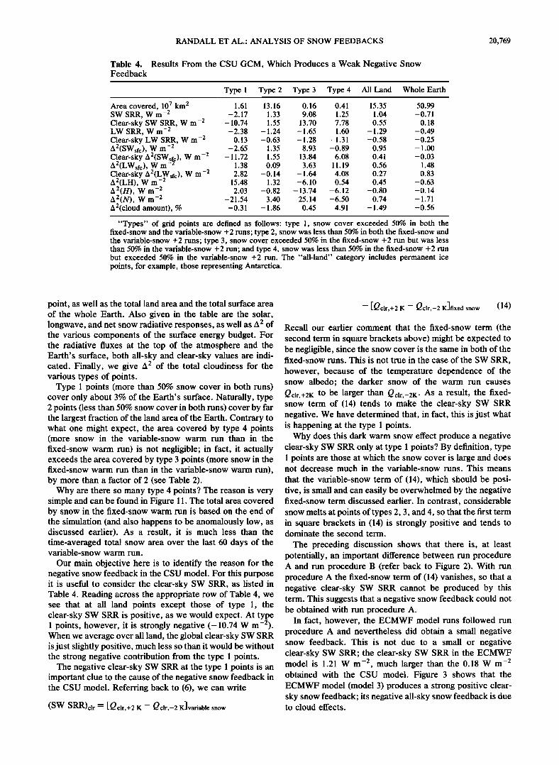
Plate 2 shows the geographical distribution of each type of point. Table 4 shows the total area covered by each type of


Table 4. Results From the CSU GCM, Which Produces a Weak Negative Snow Feedback

Type 1 Type 2 Type 3 Type 4 All Land Whole Earth

Area covered, 10 7 km 2 1.61 13.16 0.16 0.41 15.35 50.99 SW SRR, W m -2 -2.17 1.33 9.08 1.25 1.04 -0.71 Clear-sky SW SRR, W m -2 -10.74 1.55 13.70 7.78 0.55 0.18 LW SRR, W m -2 -2.38 - 1.24 - 1.65 1.60 - 1.29 -0.49 Clear-sky LW SRR, W m -2 0.13 -0.63 -1.28 -1.31 -0.58 -0.25 A2(SWsfc), W m -2 -2.65 1.35 8.93 -0.89 0.95 -1.00 Clear-sky A2(SWsfc), W m-2 - 11.72 1.55 13.84 6.08 0.41 -0.03 A 2(LWsfc), W m -:• 1.38 0.09 3.63 11.19 0.56 1.48 Clear-sky A2(LWsfc), W m -2 2.82 -0.14 -1.64 4.08 0.27 0.83 A2(LH), W m -2 15.48 -1.32 -6.10 0.54 0.45 -0.63 A 2(H), W m -2 2.03 -0.82 - 13.74 -6.12 -0.80 -0.14 A 2(N), W m -2 -21.54 3.40 25.14 -6.50 0.74 - 1.71 A2(cloud amount), % -0.31 -1.86 0.45 4.91 -1.49 -0.56

"Types" of grid points are defined as follows: type 1, snow cover exceeded 50% in both the fixed-snow and the variable-snow + 2 runs; type 2, snow was less than 50% in both the fixed-snow and the variable-snow + 2 runs; type 3, snow cover exceeded 50% in the fixed-snow + 2 run but was less than 50% in the variable-snow + 2 run; and type 4, snow was less than 50% in the fixed-snow + 2 run but exceeded 50% in the variable-snow +2 run. The "all-land" category includes permanent ice points, for example, those representing Antarctica.

point, as well as the total land area and the total surface area of the whole Earth. Also given in the table are the solar, longwave, and net snow radiative responses, as well as A2 of the various components of the surface energy budget. For the radiative fluxes at the top of the atmosphere and the Earth's surface, both all-sky and clear-sky values are indicated. Finally, we give A 2 of the total cloudiness for the various types of points.

Type 1 points (more than 50% snow cover in both runs) cover only about 3% of the Earth's surface. Naturally, type 2 points (less than 50% snow cover in both runs) cover by far the largest fraction of the land area of the Earth. Contrary to what one might expect, the area covered by type 4 points (more snow in the variable-snow warm run than in the fixed-snow warm run) is not negligible; in fact, it actually exceeds the area covered by type 3 points (more snow in the fixed-snow warm run than in the variable-snow warm run), by more than a factor of 2 (see Table 2).

Why are there so many type 4 points? The reason is very simple and can be found in Figure 11. The total area covered by snow in the fixed-snow warm run is based on the end of the simulation (and also happens to be anomalously low, as discussed earlier). As a result, it is much less than the time-averaged total snow area over the last 60 days of the variable-snow warm run.

Our main objective here is to identify the reason for the negative snow feedback in the CSU model. For this purpose it is useful to consider the clear-sky SW SRR, as listed in Table 4. Reading across the appropriate row of Table 4, we see that at all land points except those of type 1, the clear-sky SW SRR is positive, as we would expect. At type 1 points, however, it is strongly negative (-10.74 W m-2). When we average over all land, the global clear-sky SW SRR is just slightly positive, much less so than it would be without the strong negative contribution from the type 1 points.

The negative clear-sky SW SRR at the type 1 points is an important clue to the cause of the negative snow feedback in the CSU model. Referring back to (6), we can write

(SW SRR)cl r = [Qclr,+2 K -- Qclr,-2 K]variable snow

- [Qclr,+2 K -- Qclr,-2 K]fixed snow (14)

Recall our earlier comment that the fixed-snow term (the second term in square brackets above) might be expected to be negligible, since the snow cover is the same in both of the fixed-snow runs. This is not true in the case of the SW SRR,

however, because of the temperature dependence of the snow albedo; the darker snow of the warm run causes

Qclr,+2K to be larger than Qclr,-2K. As a result, the fixed- snow term of (14) tends to make the clear-sky SW SRR negative. We have determined that, in fact, this is just what is happening at the type 1 points.

Why does this dark warm snow effect produce a negative clear-sky SW SRR only at type 1 points? By definition, type 1 points are those at which the snow cover is large and does not decrease much in the variable-snow runs. This means

that the variable-snow term of (14), which should be positive, is small and can easily be overwhelmed by the negative fixed-snow term discussed earlier. In contrast, considerable snow melts at points of types 2, 3, and 4, so that the first term in square brackets in (14) is strongly positive and tends to dominate the second term.

The preceding discussion shows that there is, at least potentially, an important difference between run procedure A and run procedure B (refer back to Figure 2). With run procedure A the fixed-snow term of (14) vanishes, so that a negative clear-sky SW SRR cannot be produced by this term. This suggests that a negative snow feedback could not be obtained with run procedure A.

In fact, however, the ECMWF model runs followed run procedure A and nevertheless did obtain a small negative snow feedback. This is not due to a small or negative clear-sky SW SRR; the clear-sky SW SRR in the ECMWF model is 1.21 W m -2, much larger than the 0.18 W m -2 obtained with the CSU model. Figure 3 shows that the ECMWF model (model 3) produces a strong positive clear- sky snow feedback; its negative all-sky snow feedback is due to cloud effects.


Table 5. Results From the CSU GCM in the Fixed-Snow

Experiment and the Fixed Surface Albedo Experiment

Fixed Surface Fixed Snow Albedo

Clear-sky SW SRR, W m -2 0.18 0.59 All-sky SW SRR, W m -2 -0.71 -0.13 Clear-sky LW SRR, W m -2 -0.25 -0.45 All-sky LW SRR, W m -2 -0.49 -0.27 A 0.357 0.346

As 0.394 0.344 A/As 0.906 1.006

See text for details.

4.3. A Fixed Surface Albedo Experiment With the CSU GCM

We have repeated the "fixed-snow" +2 and -2 simulations with the CSU GCM, this time fixing the surface albedo at the fixed-snow points, as in the experiment with the BMRC model. In addition, we have chosen the fixed-snow points as those which have more than 50% snow cover as averaged over the last day of the -2 K variable-snow run, rather than using just the last time step of that run.

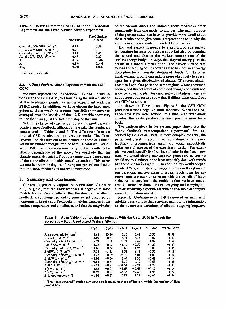
With this change of experiment design the model gives a positive snow feedback, although it is weak. The results are summarized in Tables 5 and 6. The differences from the

original CSU results are not very dramatic. The "area covered" entries turn out to be identical to those of Table 3, within the number of digits printed here. In contrast, Colman et al. [1993] found a strong sensitivity of their results to the albedo dependence of the snow. We conclude that the climate sensitivity arising from the temperature dependence of the snow albedo is highly model dependent. This raises yet another warning flag, reinforcing our general conclusion that the snow feedback is not well understood.

5. Summary and Conclusions Our results generally support the conclusions of Cess et

al. [1991], i.e., that the snow feedback is negative in some models and positive in others, that the direct snow albedo feedback is supplemented and to some extent obscured by numerous indirect snow feedbacks involving changes in the surface temperature and cloudiness, and that the magnitudes

of the various direct and indirect snow feedbacks differ

significantly from one model to another. The main purpose of the present study has been to provide more detail about these results and to give some interpretations as to why the various models responded in such different ways.

The land surface responds to a prescribed sea surface temperature increase by melting snow but also by warming the ground and altering the various components of the surface energy budget in ways that depend strongly on the details of a model's formulation. The darker surface that

follows the melting of the snow can lead to more solar energy absorption for a given distribution of clouds. On the other hand, warmer ground can radiate more effectively to space, again for a given distribution of clouds. Of course, cloudiness itself can change in the same regions where snowmelt occurs, and the net effect of combined changes of clouds and snow cover on the planetary and surface radiation budgets is not obvious; our results show that it differs drastically from one GCM to another.

As shown in Table 1 and Figure 3, the CSU GCM produced a weak negative snow feedback. When the CSU fixed-snow runs were redone, this time with fixed-snow albedos, the model produced a small positive snow feedback.

The analysis given in the present paper shows that the "snow feedback intercomparison experiment" first de- scribed by Cess et al. [1991] is more complex than we, the participants, first realized. If we were doing such a snow feedback intercomparison again, we would undoubtedly refine several aspects of the experiment design. For example, we would specify fixed surface albedos in the fixed-snow runs, we would clearly mandate run procedure B, and we would try to eliminate or at least explicitly deal with trends like those shown in Figure 11. In addition, we would adopt a standard "snow initialization procedure" as well as standard run durations and averaging intervals. Such ideas for im- provements are easy to generate with the benefit of hind- sight. At the very least, the problems that we have uncov- ered illustrate the difficulties of designing and carrying out climate sensitivity experiments with an ensemble of complex general circulation models.

Recently, Groisman et al. [1994] reported an analysis of satellite observations that provides quantitative information on the systematic variations of albedo, outgoing longwave

Table 6. As in Table 4 but for the Experiment With the CSU GCM in Which the Fixed-Snow Runs Used Fixed Surface Albedos

Type I Type 2 Type 3 Type 4 All Land Whole Earth

Area covered, 107 km z 1.61 13.16 0.16 0.41 15.35 50.99 SW SRR, W m -z 3.09 -0.84 7.74 8.55 -0.09 -0.13 Clear-sky SW SRR, W m -2 5.19 1.09 26.78 8.47 1.99 0.59 LW SRR, W m -z -1.28 -0.05 -1.10 -2.52 -0.25 -0.27 Clear-sky LW SRR, W m -z -1.66 -0.64 -5.65 -1.95 -0.83 -0.45 A2(SWsfc), W m -2 3.11 -1.15 6.58 8.13 -0.37 -0.19 Clear-sky A2(SWsfc), W m -2 5.22 0.99 26.70 8.04 1.89 0.64 A2(LWsfc), W m -z -1.80 -0.36 2.45 2.36 -0.41 -0.14 Clear-sky A2(LWsfc), W m -2 -0.54 -0.64 -3.39 0.49 -0.63 -0.29 A2(LH), W m -2 -5.03 -0.77 -33.53 -9.21 -1.79 -0.83 A2(H), W m -2 1.38 -0.01 -5.67 -7.63 -0.12 -0.14 A2(N), W m -2 8.57 -0.01 43.33 22.60 1.95 -0.74 A2(cloud amount), % - 1.30 -0.62 0.88 1.23 -0.62 -0.44

The "area covered" entries turn out to be identical to those of Table 4, within the number of digits printed here.


radiation, and surface temperature, associated with snow fluctuations in the northern hemisphere, over a 20-year period. These observed variations are related to the shortwave and longwave SRR as discussed in this paper. In the future, comparison with such observations will allow more quantitative evaluation of the realism of climate model simulations of snow forcing and snow feedback.

Acknowledgments. The FANGIO GCM intercomparison project was initiated under the auspices of the Atmospheric and Climate Research Division, U.S. Department of Energy. It has been sup- ported under grant DE-FG02-89-ER69027 to Colorado State Univer- sity, grant DE-FG0285-ER60314 to SUNY Stony Brook, inter- agency agreement DE-AI05-90ER61068 to the Goddard Institute for Space Studies, contract W-7405-ENG-48 to Lawrence Livermore National Laboratory, and contract DE-AI01-80EV10220 to the National Center for Atmospheric Research, which is sponsored by the National Science Foundation. The Lawrence Livermore Na-

tional Laboratory received support through the University of Cali- fornia Institutional Collaborative Research Program to the Scripps Institution of Oceanography. Further support was provided by NASA's Climate Program under grant NAG 1-1266 to Colorado State University, by the Bundesminister fur Forschung und Tech- nologie, Federal Republic of Germany, through grant KF20128 to the University of Hamburg, and by the Commission of European Communities to DMN/CNRM. Warren Washington of the National Center for Atmospheric Research participated in an earlier phase of this study.

References

Barnett, T. P., L. D•menil, V. Schlese, E. Roeckner, and M. Latif, The effect of Eurasian snow cover on regional and global climate variations, J. Atmos. $ci., 46, 661-685, 1989.

Budyko, M. I., The effect of solar radiation variations on the climate of the Earth, Tellus, 21,611-619, 1969.

Cess, R. D., et al., Intercomparison and interpretation of cloud- climate feedback as produced by fourteen atmospheric general circulation models, Science, 245, 513-516, 1989.

Cess, R. D., et al., Intercomparison and interpretation of climate feedback processes in 19 atmospheric general circulation models, J. Geophys. Res., 95, 16,601-16,615, 1990.

Cess, R. D., et al., Interpretation of snow-climate feedback as produced by 17 general circulation models, Science, 253,888-892, 1991.

Cess, R. D., et al., Intercomparison of CO2 radiative forcing in general circulation models, Science, 262, 1252-1255, 1993.

Colman, R. A., B. J. McAvaney, J. R. Fraser, L. J. Rikus, and R. R. Dahni, Snow and cloud feedbacks modelled by an atmospheric general circulation model, Clim. Dyn., 9, 253-265, 1994.

Crowley, T. J., and G. R. North, Paleoclimatology, 339 pp., Oxford University Press, New York, 1991.

D6qu6, M., and J. F. Royer, GCM response of the mean zonal surface heat and water budgets to a global sea surface temperature anomaly, Dyn. Atmos. Oceans, 16, 133-146, 1991.

Dey, B., and O. S. R. U. Bhanu Kumar, An apparent relationship between Eurasian snow cover and the advanced period of the Indian summer monsoon, J. Appl. Meteorol., 21, 1929-1932, 1982.

Groisman, P. Ya., T. R. Karl, and R. W. Knight, Observed impact of snow cover on the heat balance and the rise of continental

spring temperatures, Science, 263, 198-200, 1994. Hummel, J. R., and R. A. Reck, A global surface albedo model, J.

Appl. Meteorol., 18, 239-253, 1979. Ingram, W. J., C. A. Wilson, and J. F. B. Mitchell, Modeling

climate change: An assessment of sea ice and surface albedo feedbacks, J. Geophys. Res., 94, 8609-8622, 1989.

Loth, B., H.-F. Graf, and J. M. Oberhuber, Snow cover model for

global climate simulations, J. Geophys. Res., 98, 10,451-10,464, 1993.

Mintz, Y., and V. Serafini, Monthly normal global fields of soil moisture and land-surface evapotranspiration, paper presented at Symposium on Variations in the Global Water Budget, Paleoclim. Comm. of the Int. Union for Quat. Res., Oxford, England, Aug. 10-15, 1981.

Randall, D. A., et al., Intercomparison and interpretation of surface energy fluxes in atmospheric general circulation models, J. Geo- phys. Res., 97, 3711-3724, 1992.

Robock, A., The seasonal cycle of snow cover, sea ice, and surface albedo, Mon. Weather Rev., 108, 267-285, 1980.

Robock, A., Ice and snow feedbacks and the latitudinal and seasonal distribution of climate sensitivity, J. Atmos. $ci., 40, 986-997, 1983.

Schlesinger, M. E., Quantitative analysis of feedbacks in climate model simulations, in Understanding Climate Change, Geophys. Monogr. $er., vol. 52, edited by A. L. Berger, R. E. Dickinson, and J. Kidson, pp. 177-187, AGU, Washington, D.C., 1989.

Sellers, W. D., A global climatic model based on the energy balance of the earth-atmosphere system, J. Appl. Meteorol., 8, 392-400, 1969.

Yasunari, T., A. Kitoh, and T. Tokioka, Local and remote responses to excessive snow mass over Eurasia appearing in the northern spring and summer climate: A study with the MRI GCM, J. Meteorol. $oc. Jpn., 69, 473-487, 1991.

J.P. Blancbet, Physics Department, University of Quebec in Montreal, P.O. Box 8888, Station A, Montreal, Quebec, Canada H3C 3P8.

R. D. Cess and M.-H. Zhang, Institute for Terrestrial and Plane- tary Atmospheres, Marine Sciences Research Center, State Univer- sity of New York at Stony Brook, Stony Brook, NY 11794-5000.

S. Chalita and H. Le Treut, Laboratoire de Meteorologie Dy- namique, Ecole Polytechnique, 91128 Palaiseau, Paris, France.

R. Coleman, B. J. McAvaney, and L. Rikus, Bureau of Meteo- rology Research Centre, P.O. Box 1289K, GPO Melbourne 3001, Australia.

D. Dazlich and D. Randall, Department of Atmospheric Science, Colorado State University, Ft. Collins, CO 80523.

A.D. Del Genio and A. Lacis, NASA Goddard Institute for Space Flight, 2880 Broadway, New York, NY 10025.

E. Keup, E. Roechner, and U. Schlese, Meteorologisches Insti- tut, University of Hamburg, Bundesstrasse 55, D-2000, Hamburg 13, Germany.

X.-Z. Liang, Atmospheric Sciences Research Center, 100 Fuller Road, State University of New York at Albany, Albany, NY 12205.

J. F. Mahfouf and J. F. Royer, Direction de la Meteorologie, Centre National de Recherches Meteorologie, 42 Avenue Gustave Coriolis, Toulouse 31057, France.

V. P. Meleshko, Voeikov Main Geophysical Observatory, St. Petersburg, Russia.

J.-J. Morcrette, European Center for Medium-Range Weather Forecasts, Shinfield Park, Reading, Berkshire RG2 9AX, England.

P.M. Norris, Climate Research Group, Scripps Institution of Oceanography, University of California, San Diego, 9500 Gilman Drive, 0224, La Jolla, CA 92093-0224.

G. L. Potter and K. E. Taylor, Lawrence Livermore National Laboratory, P.O. Box 808, L-262, Livermore, CA 94550.

D. A. Sheinin, National Meteorological Center, World Weather Building, Washington, DC 20233.

A. P. Sokolov, Department of Earth, Atmospheric and Planetary Sciences, Massachusetts Institute of Technology, Cambridge, MA 02139.

R. T. Wetheraid, NOAA Geophysical Fluid Dynamics Labora- tory, Princeton University, P.O. Box 308, Princeton, NJ 08542.

I. Yagai, Meteorological Research Institute, 1-1 Nagamine, Yat- abe, Isukoba-Gun, Ibaraki-ken, 305 Japan.

(Received October 6, 1993; revised June 17, 1994; accepted June 17, 1994.)

Documents

Analysis of snow feedbacks in 14 GCMs (1994)