Analysis of the Technical Efficiency of Urban Bus Services in Spain Based on SBM Models

International Scholarly Research NetworkISRN Civil EngineeringVolume 2012, Article ID 984758, 13 pagesdoi:10.5402/2012/984758

Research Article

Analysis of the Technical Efficiency of Urban Bus Services inSpain Based on SBM Models

Pablo Jorda,1 Rocıo Cascajo,2 and Andres Monzon2

1 Universidad Politecnica de Madrid, Escuela Tecnica Superior de Ingenieros de Caminos, Canales y Puertos, 28040 Madrid, Spain2 TRANSyT-Transport Research Centre, Universidad Politecnica de Madrid, 28040 Madrid, Spain

Correspondence should be addressed to Pablo Jorda, [email protected]

Received 29 February 2012; Accepted 8 May 2012

Academic Editor: J. D. Nelson

Copyright © 2012 Pablo Jorda et al. This is an open access article distributed under the Creative Commons Attribution License,which permits unrestricted use, distribution, and reproduction in any medium, provided the original work is properly cited.

During the first decade of the new millennium, fueled by the economic development in Spain, urban bus services were extended.Since the years 2008 and 2009, the root of the economic crisis, the improvement of these services is at risk due to economicproblems. In this paper, the technical efficiency of the main urban bus companies in Spain during the 2004–2009 period arestudied using SBM (slack-based measures) models and by establishing the slacks in the services’ production inputs. The influenceof a series of exogenous variables on the operation of the different services is also analyzed. It is concluded that only the 24% ofthe case studies are efficient, and some urban form variables can explain part of the inefficiency. The methodology used allowsstudying the inefficiency in a disaggregated way that other DEA (data envelopment analysis) models do not.

1. Introduction

The flexibility in the management offered by buses is themain cause of their success compared to other modes, suchas rail. Urban public transport offered by buses allows forthe completion of different activities, be it work, education,shopping, leisure, and so forth. The services are, then, afundamental pillar of society. This leads, in the main Spanishcities, to services being offered by one or a few publiccompanies, without any competition from other companies.This lack of competition can bring about a complacency inmanagement, or the need to improve the efficiency of theservices.

The evaluation of the operational efficiency of an urbanbus service is a complicated task. One must identify thoseelements which are decisive in the operating of the system,in order to subsequently define a model which, on thebase of these decisive elements, reflects its functions in asimplified manner. In the evaluation of a service, therefore,one should consider the consumption of resources (inputs)when obtaining the results or production (outputs).

Beginning with these ideas, and aided by the informationsupplied by the database of the Spanish MetropolitanMobility Observatory (MMO) [1–8], this paper will discuss

the problem of studying the technical efficiency of urban busservices, considering the greater number of evaluation crite-ria related to the socioeconomic context and the evolution ofpublic transport networks [9].

2. Analysis of Technical Efficiency withthe DEA Method

The Data Envelopment Analysis (DEA) is a linear pro-gramming method whose object is to calculate the relativeefficiencies of a group of decision-making units (DMUs).These DMUs can be, as in the case of this investigation, urbanbus companies or, more specifically, a bus company in a givenyear.

The DEA is one of the existing frontier methods. Frontiermethods are those in which an efficiency frontier is used toclassify the different DMUs. The efficiency frontier is basedon real observations and only the cases of best practicesbelong to it. All DMUs that are not on the frontier areconsidered inefficient.

When assessing the efficiency of urban bus companies, inaddition to the DEA method, other methodologies have beenused. The stochastic parametric methodologies has been

2 ISRN Civil Engineering

Table 1: Frontier methodologies.

Functionalform

Measurement error

Deterministic Stochastic

ParametricCorrectedOLS, and soforth

Frontiers with explicitassumptions (exponential, halfnormal, etc.) for the technicalefficiency distributions

Nonparametric

FDH,DEA-typemodels, and soforth

Resampling, chance-constrained programming, andso forth

Source: [10].

widely used [9, 10], as well as other frontier methodologies(see Table 1).

CCR and BCC models were the first DEA models to beformulated and are explained below. All subsequent DEAmodels have been developed from them.

Given the group of DMUs K, the technical efficiencyof the DMU k0 is defined as the ratio of the weightedsum of its n outputs yjk0 and the weighted sum m of itsinputs xjk0, all expressed as positive values. As outputs, inthe case of buses companies, it can be used vehicle-kmor pax-km. As inputs, the variables most commonly usedare number of buses, number of workers, companies costs,and infrastructure variables The problem of the fractionalprogramming, known as the CCR model [14], is expressedas follows:

Maximize h0 =∑n

j=1 wj yjk0∑m

i=1 vixik0

Subject to:∑n

j=1 wj yjk0∑m

i=1 vixik0≤ 1 wj , vi > 0,

i = 1, . . . ,m; j = 1, . . . ,n; k = 1, . . . ,K ,

(1)

where the subindex i numbers the inputs, the j outputs, andthe k the DMUs. wj and vi are weights.

The first restriction of this problem indicates that theefficiency value of each unit k, in function of the givenweights, should be, at most, one. If one observes the objectivefunction, its end is to maximize the relationship between avirtual output, composed of all considered outputs, and avirtual input that is also a compilation of various inputs. Thesecond condition requires that the weights of the outputs andinputs wj and vi be greater than zero. This restriction seeksto prevent the outputs or inputs of the DMUs from varyingwith total freedom. In the analysis, the unit k0 is inefficientwith respect to the rest of the DMUs if it does not reach aratio of outputs to inputs equal to one.

In order to resolve the problem expressed in (1), themodel is transformed and expressed as an equivalent linearform [14, 15]. The resulting input-oriented model enablesevaluations of DMUs in constant returns to scale (CRS)

situation. It is named as envelopment model [16] andexpressed in the following form:

Minimize h0 = θ0

Subject to:

K∑

k=1

λkxik = θ0xik0, 0 ≤ θ0 ≤ 1,

K∑

k=1

λk yjk = yjk0,

λk ≥ 0,

i = 1, . . . ,m; j = 1, . . . ,n; k = 1, . . . ,K.

(2)

The first restriction of this problem indicates that thenumber of inputs used by the DMU k0, multiplied by theefficiency factor θ0, should be equal to the number of inputsused by the reference unit of the DMU k0 at the frontier,which is composed of other DMUs of the K group. Thatis to say, its capacity to transform inputs into outputs willbe equal to or less than the capacity of the reference unit.The third restriction indicates that the reference unit at thefrontier should produce the same number of outputs as thek0 unit.

The intensity of the efficiency factor can, therefore, beused to determine the minimum quantity of use of inputsthat must be proportionally reduced for the k0 unit to beefficient. The efficiency factor θ0 has values of between zeroand one, both included. The units that contribute to theconstruction of the reference unit at the frontier will haveweight values λk different from zero.

CCR models (2) make it possible to evaluate a group ofDMUs that have constant returns to scale. However, thereare DMUs with increasing returns to scale, others decreasing,and others constant. Therefore, in [15] they reformulatedthe CCR model to allow for variable returns to scale, thusdefining a new model, the BCC. This model is expressed inthe following manner:

Minimize h0 = θ0

Subject to:

K∑

k=1

λkxik = θ0xik0, 0 ≤ θ0 ≤ 1,

K∑

k=1

λk yjk = yjk0,

K∑

k=1

λk = 1,

λk ≥ 0,

i = 1, . . . ,m; j = 1, . . . ,n; k = 1, . . . ,K.

(3)

ISRN Civil Engineering 3

Table 2: Advantages and disadvantages of DEA.

Advantages Disadvantages

Simultaneous analysis of outputsand inputs

Ignores the effect of exogenousvariables on the operation

It is not necessary, a priori, todefine the frontier form

Ignores statistical errors

Relative efficiency, compared tothe best observation

Does not say how to improveefficiency

Need no information on pricesDifficult to perform statisticaltests with the results

Source: [11–13].

It is an input-oriented BCC model [11]. The onlydifference from the CCR model (2) is that a new conditionis included: the summation of the weights λk is equal toone. This makes it possible to evaluate the variable returnsto scale (VRS) in the DMUs and guarantees that each DMUis compared only with those of a similar size [17] to keepthem from being considered inefficient simply because of thedifferences of scale between DMUs.

Finally, in Table 2 are shown the main advantages anddisadvantages of the DEA method over other methods, likethe stochastic parametric methodologies.

The lack of information on prices in the database used isone of the reasons why in this study is used the DEA methodinstead of the stochastic parametric methodologies.

3. Slacks and SBM Models

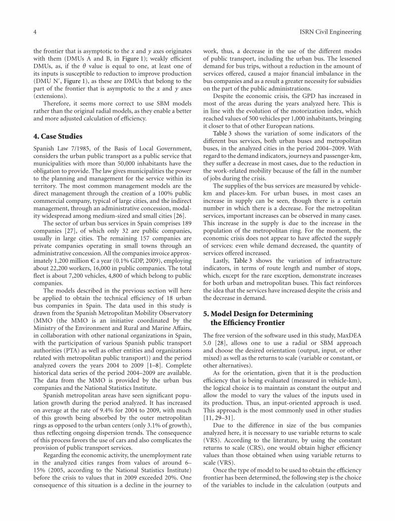
In some cases, and in order for a DMU k0 to reach efficiency,the proportional reduction of inputs achieved using theθ factor is not enough, as has been indicated in models(2) and (3). An additional reduction of input is necessary,or an additional output increase, as it is not proportional(radial). These complementary adjustments to the inputs(si−) (excess of input) or to the outputs (s j+) (outputshortfall) are together known as slacks [18]. Figure 1 clarifiesthese concepts.

Thus, given a frontier, the efficiency of the DMU Mis evaluated, projecting it toward the frontier in a radialmanner in the direction OM, and does not produce aproblematic situation, as the slacks of the projection M′

are zero. No additional reduction of inputs is necessary toachieve efficiency. For the DMU N, projected radially towardthe frontier, it can be observed that its projection N′ mustconsume the same quantity of input 1 as the DMU B, butit consumes a greater quantity of input 2 (segment BN′), forwhich it cannot be considered equally efficient to the DMU B.

So, it is not acceptable to measure the efficiency ofa group of DMUs only by means of the radial factor θ.The slacks must also be kept in mind when evaluating theefficiency value of the DMUs.

Some modifications must be introduced to the linearproblem of the CCR model (2) to be able to evaluate theslacks. For a case of orientation to the input, once the slackshave been included, the resulting model is that proposed

Input 1

Input 2

A

B

N

M

O

M

N

Figure 1: Radial projection and slacks. Input-input representation.Source: based on [19].

in [15]:

Minimize h0 = θ0 − ε

⎛

⎝n∑

j=1

s j+ +

m∑

i=1

si−⎞

⎠,

Subject to:

K∑

k=1

λkxik + si− = θ0xik0, 0 ≤ θ0 ≤ 1,

K∑

k=1

λk yjk − s j+ = yjk0,

λk, si−, s j+ ≥ 0,

ε > 0, very small value

i = 1, . . . ,m; j = 1, . . . ,n; k = 1, . . . ,K.

(4)

Thus, the problem (4) also gives as results values of theefficiency factor θ0 between zero and one. Additionally, anddiffering from the previous models, it provides the valuesof the vectors of slacks s j− and s j+, which can be equal toor greater than zero. In subsequent models, the parameter εceases to be utilized.

Based on several works [12, 18, 20–24], many modelshave been developed that include slacks when assessing theefficiency factor; these are known as Slacks-Based Measuresor SBM.

If one maintains the original criterion that a DMU isefficient if it is on a frontier (θ0 = 1), independentlyof the values of its slacks, there can be different typesof efficiency in the DMUs. In [25] it is described up tothree different categories: efficient DMUs, which fulfill therequirement that θ is equal to one and its slacks are zero(DMU M′, in Figure 1); extremely efficient DMUs, withthe same characteristics as an efficient one, the part of


the frontier that is asymptotic to the x and y axes originateswith them (DMUs A and B, in Figure 1); weakly efficientDMUs, as, if the θ value is equal to one, at least one ofits inputs is susceptible to reduction to improve production(DMU N′, Figure 1), as these are DMUs that belong to thepart of the frontier that is asymptotic to the x and y axes(extensions).

Therefore, it seems more correct to use SBM modelsrather than the original radial models, as they enable a betterand more adjusted calculation of efficiency.

4. Case Studies

Spanish Law 7/1985, of the Basis of Local Government,considers the urban public transport as a public service thatmunicipalities with more than 50,000 inhabitants have theobligation to provide. The law gives municipalities the powerto the planning and management for the service within itsterritory. The most common management models are thedirect management through the creation of a 100% publiccommercial company, typical of large cities, and the indirectmanagement, through an administrative concession, modal-ity widespread among medium-sized and small cities [26].

The sector of urban bus services in Spain comprises 189companies [27], of which only 32 are public companies,usually in large cities. The remaining 157 companies areprivate companies operating in small towns through anadministrative concession. All the companies invoice approx-imately 1,200 million C a year (0.1% GDP, 2009), employingabout 22,200 workers, 16,000 in public companies. The totalfleet is about 7,200 vehicles, 4,800 of which belong to publiccompanies.

The models described in the previous section will herebe applied to obtain the technical efficiency of 18 urbanbus companies in Spain. The data used in this study isdrawn from the Spanish Metropolitan Mobility Observatory(MMO (the MMO is an initiative coordinated by theMinistry of the Environment and Rural and Marine Affairs,in collaboration with other national organizations in Spain,with the participation of various Spanish public transportauthorities (PTA) as well as other entities and organizationsrelated with metropolitan public transport)) and the periodanalyzed covers the years 2004 to 2009 [1–8]. Completehistorical data series of the period 2004–2009 are available.The data from the MMO is provided by the urban buscompanies and the National Statistics Institute.

Spanish metropolitan areas have seen significant popu-lation growth during the period analyzed. It has increasedon average at the rate of 9.4% for 2004 to 2009, with muchof this growth being absorbed by the outer metropolitanrings as opposed to the urban centers (only 3.1% of growth),thus reflecting ongoing dispersion trends. The consequenceof this process favors the use of cars and also complicates theprovision of public transport services.

Regarding the economic activity, the unemployment ratein the analyzed cities ranges from values of around 6–15% (2005, according to the National Statistics Institute)before the crisis to values that in 2009 exceeded 20%. Oneconsequence of this situation is a decline in the journey to

work, thus, a decrease in the use of the different modesof public transport, including the urban bus. The lesseneddemand for bus trips, without a reduction in the amount ofservices offered, caused a major financial imbalance in thebus companies and as a result a greater necessity for subsidieson the part of the public administrations.

Despite the economic crisis, the GPD has increased inmost of the areas during the years analyzed here. This isin line with the evolution of the motorization index, whichreached values of 500 vehicles per 1,000 inhabitants, bringingit closer to that of other European nations.

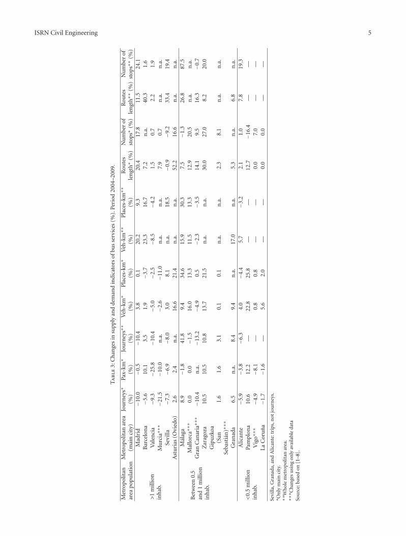
Table 3 shows the variation of some indicators of thedifferent bus services, both urban buses and metropolitanbuses, in the analyzed cities in the period 2004–2009. Withregard to the demand indicators, journeys and passenger-km,they suffer a decrease in most cases, due to the reduction inthe work-related mobility because of the fall in the numberof jobs during the crisis.

The supplies of the bus services are measured by vehicle-km and places-km. For urban buses, in most cases anincrease in supply can be seen, though there is a certainnumber in which there is a decrease. For the metropolitanservices, important increases can be observed in many cases.This increase in the supply is due to the increase in thepopulation of the metropolitan ring. For the moment, theeconomic crisis does not appear to have affected the supplyof services: even while demand decreased, the quantity ofservices offered increased.

Lastly, Table 3 shows the variation of infrastructureindicators, in terms of route length and number of stops,which, except for the rare exception, demonstrate increasesfor both urban and metropolitan buses. This fact reinforcesthe idea that the services have increased despite the crisis andthe decrease in demand.

5. Model Design for Determiningthe Efficiency Frontier

The free version of the software used in this study, MaxDEA5.0 [28], allows one to use a radial or SBM approachand choose the desired orientation (output, input, or othermixed) as well as the returns to scale (variable or constant, orother alternatives).

As for the orientation, given that it is the productionefficiency that is being evaluated (measured in vehicle-km),the logical choice is to maintain as constant the output andallow the model to vary the values of the inputs used inits production. Thus, an input-oriented approach is used.This approach is the most commonly used in other studies[11, 29–31].

Due to the difference in size of the bus companiesanalyzed here, it is necessary to use variable returns to scale(VRS). According to the literature, by using the constantreturns to scale (CRS), one would obtain higher efficiencyvalues than those obtained when using variable returns toscale (VRS).

Once the type of model to be used to obtain the efficiencyfrontier has been determined, the following step is the choiceof the variables to include in the calculation (outputs and


Ta

ble

3:C

han

ges

insu

pply

and

dem

and

indi

cato

rsof

bus

serv

ices

(%).

Peri

od20

04–2

009.

Met

ropo

litan

area

popu

lati

onM

etro

polit

anar

ea(m

ain

city

)Jo

urn

eys∗

(%)

Pax-

km∗

(%)

Jou

rney

s∗∗

(%)

Veh

-km∗

(%)

Pla

ces-

km∗

(%)

Veh

-km∗∗

(%)

Pla

ces-

km∗∗

(%)

Rou

tes

len

gth∗

(%)

Nu

mbe

rof

stop

s∗(%

)R

oute

sle

ngt

h∗∗

(%)

Nu

mbe

rof

stop

s∗∗

(%)

>1

mill

ion

inh

ab.

Mad

rid

−10.

0−0

.5−1

0.4

3.8

0.1

20.2

9.3

20.4

17.8

11.5

24.1

Bar

celo

na

−5.6

10.1

3.5

1.9

−3.7

23.3

16.7

7.2

n.a

.40

.31.

6V

alen

cia

−9.3

−25.

8−1

0.4

−5.0

−2.5

−8.5

−4.2

1.5

0.7

2.2

1.9

Mu

rcia∗∗∗

−21.

5−1

0.0

n.a

.−2

.6−1

1.0

n.a

.n

.a.

7.9

0.7

n.a

.n

.a.

Sevi

lla−7

.3−6

.9−8

.03.

08.

1n

.a.

18.5

−0.9

−9.2

33.4

19.4

Ast

uri

as(O

vied

o)2.

62.

4n

.a.

16.6

21.4

n.a

.n

.a.

52.2

16.6

n.a

.n

.a.

Bet

wee

n0.

5an

d1

mill

ion

inh

ab.

Mal

aga

8.9

−1.8

41.8

9.4

34.6

15.9

30.3

7.5

−1.3

26.8

87.5

Mal

lorc

a∗∗∗

0.0

0.0

−1.5

16.0

13.3

11.5

13.3

12.9

20.5

n.a

.n

.a.

Gra

nC

anar

ia∗∗∗

−10.

4n

.a.

−13.

2−4

.90.

5−2

.3−3

.514

.19.

516

.3−0

.7Z

arag

oza

10.5

10.5

10.8

13.7

21.5

n.a

.n

.a.

30.0

27.0

8.2

20.0

Gip

uzk

oa(S

anSe

bast

ian

)∗∗∗

1.6

1.6

3.1

0.1

0.1

n.a

.n

.a.

2.3

8.1

n.a

.n

.a.

Gra

nad

a6.

5n

.a.

8.4

9.4

n.a

.17

.0n

.a.

5.3

n.a

.6.

8n

.a.

<0.

5m

illio

nin

hab

.

Alic

ante

−5.9

−3.8

−6.3

4.0

−4.4

5.7

−3.2

2.1

1.0

7.8

19.3

Pam

plon

a10

.612

.2—

22.8

25.8

——

12.7

−16.

4—

—V

igo∗

∗∗−4

.9−8

.1—

0.8

0.8

——

0.0

7.0

——

LaC

oru

na

−1.7

−1.6

—5.

62.

0—

—0.

00.

0—

—

Sevi

lla,G

ran

ada,

and

Alic

ante

:tri

ps,n

otjo

urn

eys.

∗ On

lym

ain

city

.∗∗

Wh

ole

met

rop

olit

anar

ea.

∗∗∗ C

han

ges

usi

ng

only

avai

labl

eda

taSo

urc

e:ba

sed

on[1

–8].


inputs). In the literature considered here, two variables areused as outputs: vehicle-km, which is the supply indicator,and pax-km, which reflects the service demand [29, 32, 33].However, the first of the two indicators is the most widelyused, though authors that have the second at their disposaluse it as well and compare the results [30, 32–36].

As for the inputs that are commonly employed, variablesare selected that can be used in a Cobb-Douglas [37]formula: work, capital, and consumption/cost variables. Asthe variable reflecting the work factor, the number of workersis commonly used, but this variable is not available in thedatabase used here. As the variable for the capital factor, thesize of the fleet is used. And finally, the operating costs of theurban bus companies are used as the variable to representconsumption.

In this study, the desired approach will differ fromthat proposed by others, including variables that reflect theinfrastructure used in the provision of services. Some authorsuse variables related to infrastructure, such as routes length,distance between stops, or network-km [29, 32, 38] butinclude them in the models as exogenous variables. In [39]it is the first time that routes length is introduced as an inputin the models. Subsequently, [36, 40] also use infrastructurevariables (routes length and number of stops) as input.

Finally, an infrastructure variable and some of the classicvariables from the Cobb-Douglas models are used for thefinal formulation of the efficiency:

θ = f (uVK)f (v1RL, v2NV, v3CC)

, (5)

where VK is the vehicle-km, RL is the routes length, NV isthe number of vehicles, CC is the company costs, and u, v1,v2, and v3 are model coefficients.

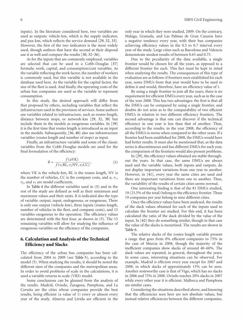
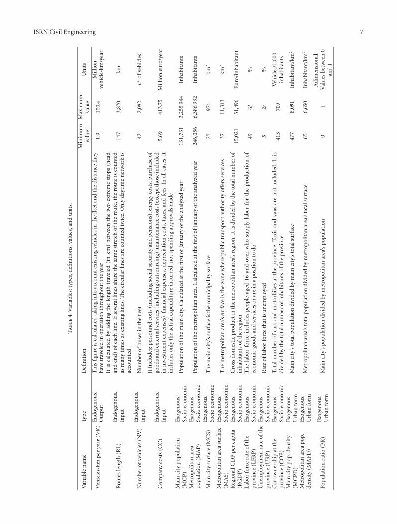
In Table 4 the different variables used in (5) and in therest of the study are defined as well as their minimum andmaximum values and their units. It is indicated also the typeof variable: output, input, endogenous, or exogenous. Thereis only one output (vehicle-km), three inputs (routes length,number of vehicles in the fleet, and company costs), and 15variables exogenous to the operation. The efficiency valuesare determined with the first four, as shown in (5). The 15remaining variables will allow for studying the influence ofexogenous variables on the efficiency of the companies.

6. Calculation and Analysis of the TechnicalEfficiency and Slacks

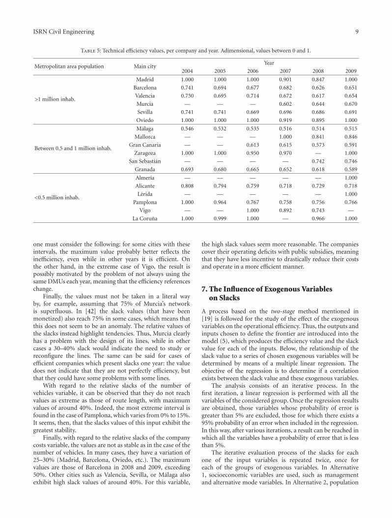
The efficiency of the urban bus companies has been cal-culated from 2004 to 2009 (see Table 5), according to themodel (5). When studying the results, it should be noted thedifferent sizes of the companies and the metropolitan areas.In order to avoid problems of scale in the calculations, it isused a variable returns to scale (VRS) model.

Some conclusions can be gleaned from the analysis ofthe results. Madrid, Oviedo, Zaragoza, Pamplona, and LaCoruna are the cities whose companies provide the bestresults, being efficient (a value of 1) every or almost everyyear of the study. Almeria and Lerida are efficient in the

only year in which they were studied, 2009. On the contrary,Malaga, Granada, and Las Palmas de Gran Canaria havea negative tendency every year, with their bus companiesachieving efficiency values in the 0.5 to 0.7 interval everyyear of the study. Large cities such as Barcelona and Valenciademonstrate modest results of between 0.65 and 0.75.

Due to the peculiarity of the data available, a singlefrontier would be chosen for all the years, as opposed to adifferent frontier for each. This fact must be kept in mindwhen analyzing the results. The consequences of this type ofevaluation are as follows: if frontiers were established for eachyear, some DMUs from that year would have to be used todefine it and would, therefore, have an efficiency value of 1.

By using a single frontier to join all the years, there is norequirement for efficient DMUs every year, such as in the caseof the year 2008. This has two advantages: the first is that allthe DMUs can be compared by using a single frontier, anddoubts do not arise as to the comparability of two efficientDMUs in relation to two different efficiency frontiers. Thesecond advantage is that one can discover if the technicalefficiency in one year is less than that of another. Thus,according to the results, in the year 2008, the efficiency ofall the DMUs is worse when compared to the other years. If afrontier had been established for 2008, the DMUs would havehad better results. It must also be mentioned that, as the dataseries is discontinuous and has different DMUs for each year,the comparison of the frontiers would also present problems.

In [29], the efficiency values obtained are stable through-out the years. In that case, the same DMUs are alwaysused and the variable values, both inputs and outputs, donot display important variations from one year to another.However, in [41], every year the same cities are used andthere are important variations from one to another. Thus,the variability of the results of certain cities seems normal.

One interesting finding is that of the 81 DMUs studied,19 (23.5% of the total) belong to the efficiency frontier. These19 companies per year belong to nine different cities.

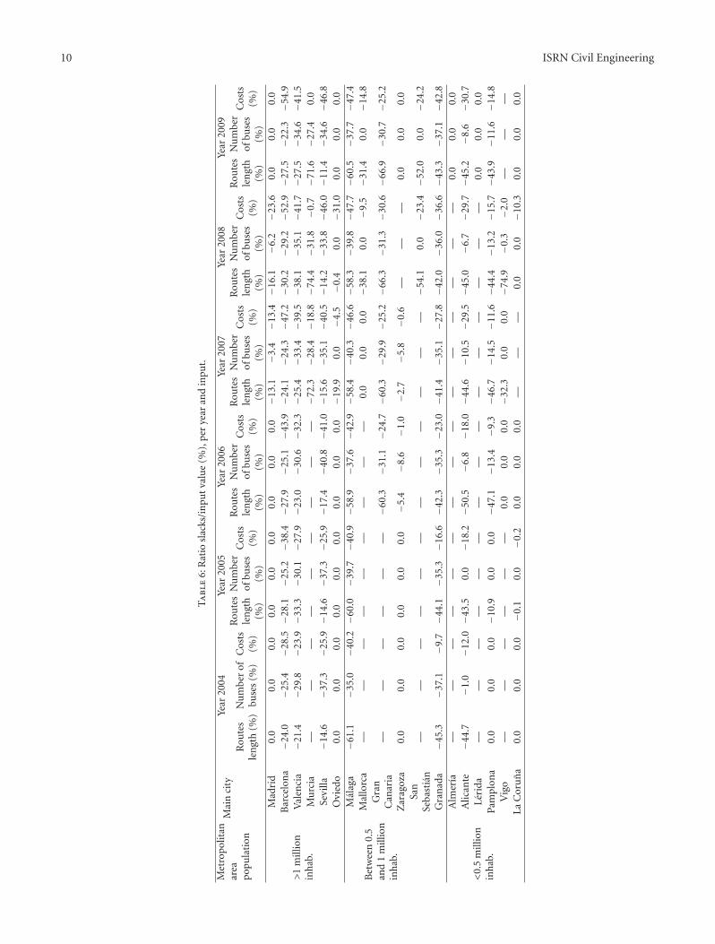
Once the efficiency values have been analyzed, the resultsof the slack values obtained for each of the inputs used tocalculate the frontier are studied. For this end, it has beencalculated the ratio of the slack divided by the value of theinput. In [42] they do something similar, though in that casethe value of the slacks is monetized. The results are shown inTable 6.

The relative slacks of the routes length variable presenta range that goes from 0% efficient companies to 75% inthe case of Murcia in 2008, though the majority of theinefficient companies show slacks of around 40–60%. Theslack values are repeated, in general, throughout the years.In some cases, interesting situations can be observed. Forexample, Madrid is efficient every year except for 2007 and2008, in which slacks of approximately 15% can be seen.Another noteworthy case is that of Vigo, which has no slacksin 2006 and 75% in 2008. Oviedo reaches 20% slacks in 2007while every other year it is efficient. Mallorca and Pamplonaare similar cases.

Considering the situations described above, and knowingthat the efficiencies seen here are not absolute values, butinstead relative efficiencies between the different companies,


Ta

ble

4:V

aria

bles

:typ

es,d

efin

itio

ns,

valu

es,a

nd

un

its.

Var

iabl

en

ame

Type

Defi

nit

ion

Min

imu

mva

lue

Max

imu

mva

lue

Un

its

Veh

icle

s-km

per

year

(VK

)E

ndo

gen

ous.

Ou

tpu

tT

his

figu

reis

calc

ula

ted

taki

ng

into

acco

un

tex

isti

ng

veh

icle

sin

the

flee

tan

dth

edi

stan

ceth

eyh

ave

trav

eled

inop

erat

ion

thro

ugh

out

the

year

1.9

100.

4M

illio

nve

hic

le-k

m/y

ear

Rou

tes

len

gth

(RL)

En

doge

nou

s.In

put

Itis

calc

ula

ted

byad

din

gth

ele

ngt

htr

avel

ed(i

nkm

)be

twee

nth

etw

oex

trem

est

ops

(hea

dan

den

d)of

each

line.

Ifse

vera

llin

essh

are

the

sam

est

retc

hof

the

rou

te,t

he

rou

teis

cou

nte

das

man

yti

mes

asex

isti

ng

lines

.Th

eci

rcu

lar

lines

are

cou

nte

dtw

ice.

On

lyda

ytim

en

etw

ork

isac

cou

nte

d

147

3,87

0km

Nu

mbe

rof

veh

icle

s(N

V)

En

doge

nou

s.In

put

Nu

mbe

rof

buse

sin

the

flee

t42

2,09

2n◦

ofve

hic

les

Com

pany

cost

s(C

C)

En

doge

nou

s.In

put

ItIn

clu

des:

per

son

nel

cost

s(i

ncl

udi

ng

soci

alse

curi

tyan

dp

ensi

ons)

,en

ergy

cost

s,pu

rch

ase

ofgo

ods

and

exte

rnal

serv

ices

(in

clu

din

gou

tsou

rcin

g),m

ain

ten

ance

cost

s(e

xcep

tth

ose

incl

ude

din

inve

stm

ent

expe

nse

s),fi

nan

cial

expe

nse

s,de

prec

iati

onco

sts,

taxe

s,an

dfe

es.I

nal

lcas

es,i

tin

clu

des

only

the

actu

alex

pen

ditu

rein

curr

ed,n

otsp

endi

ng

appr

oval

sm

ade

5.69

413.

75M

illio

neu

ro/y

ear

Mai

nci

typo

pula

tion

(MC

P)

Exo

gen

ous.

Soci

oec

onom

icPo

pula

tion

ofth

em

ain

city

.Cal

cula

ted

atth

efi

rst

ofJa

nu

ary

ofth

ean

alyz

edye

ar13

1,73

13,

255,

944

Inh

abit

ants

Met

ropo

litan

area

popu

lati

on(M

AP

)E

xoge

nou

s.So

cio

econ

omic

Popu

lati

onof

the

met

ropo

litan

area

.Cal

cula

ted

atth

efi

rst

ofJa

nu

ary

ofth

ean

alyz

edye

ar24

6,05

66,

386,

932

Inh

abit

ants

Mai

nci

tysu

rfac

e(M

CS)

Exo

gen

ous.

Soci

oec

onom

icT

he

mai

nci

ty’s

surf

ace

isth

em

un

icip

alit

ysu

rfac

e25

974

km2

Met

ropo

litan

area

surf

ace

(MA

S)E

xoge

nou

s.So

cio

econ

omic

Th

em

etro

polit

anar

ea’s

surf

ace

isth

ezo

ne

wh

ere

publ

ictr

ansp

ort

auth

orit

yoff

ers

serv

ices

3711

,313

km2

Reg

ion

alG

DP

per

capi

ta(R

GD

P)

Exo

gen

ous.

Soci

oec

onom

icG

ross

dom

esti

cpr

odu

ctin

the

met

ropo

litan

area

’sre

gion

.It

isdi

vide

dby

the

tota

lnu

mbe

rof

inh

abit

ants

ofth

ere

gion

15,0

2131

,496

Eu

ro/i

nh

abit

ant

Labo

rfo

rce

rate

ofth

epr

ovin

ce(L

FRP

)E

xoge

nou

s.So

cio

econ

omic

Th

ela

bor

forc

ein

clu

des

peo

ple

aged

16an

dov

erw

ho

supp

lyla

bor

for

the

prod

uct

ion

ofec

onom

icgo

ods

and

serv

ices

orar

ein

apo

siti

onto

do49

65%

Un

empl

oym

ent

rate

ofth

epr

ovin

ce(U

RP

)E

xoge

nou

s.So

cio

econ

omic

Rat

eof

labo

rfo

rce

that

isu

nem

ploy

ed5

28%

Car

own

ersh

ipat

the

prov

ince

(CO

P)

Exo

gen

ous.

Soci

oec

onom

icTo

tal

nu

mbe

rof

cars

and

mot

orbi

kes

atth

epr

ovin

ce.

Taxi

san

dva

ns

are

not

incl

ude

d.It

isdi

vide

dby

the

tota

lnu

mbe

rof

inh

abit

ants

ofth

epr

ovin

ce41

370

9V

ehic

les/

1,00

0in

hab

itan

tsM

ain

city

pop.

den

sity

(MC

PD

)E

xoge

nou

s.U

rban

form

Mai

nci

ty’s

tota

lpop

ula

tion

divi

ded

bym

ain

city

’sto

tals

urf

ace

477

8,09

1In

hab

itan

t/km

2

Met

ropo

litan

area

pop.

den

sity

(MA

PD

)E

xoge

nou

s.U

rban

form

Met

ropo

litan

area

’sto

talp

opu

lati

ondi

vide

dby

met

ropo

litan

area

’sto

tals

urf

ace

656,

650

Inh

abit

ant/

km2

Popu

lati

onra

tio

(PR

)E

xoge

nou

s.U

rban

form

Mai

nci

ty’s

popu

lati

ondi

vide

dby

met

ropo

litan

area

’spo

pula

tion

01

Adi

men

sion

al.

Val

ues

betw

een

0an

d1


Ta

ble

4:C

onti

nu

ed.

Var

iabl

en

ame

Type

Defi

nit

ion

Min

imu

mva

lue

Max

imu

mva

lue

Un

its

Surf

ace

rati

o(S

R)

Exo

gen

ous.

Urb

anfo

rmM

ain

city

’ssu

rfac

edi

vide

dby

met

ropo

litan

area

’ssu

rfac

e0

1A

dim

ensi

onal

.V

alu

esbe

twee

n0

and

1

Man

agem

ent

(PR

IV)

Exo

gen

ous.

Man

agem

ent

and

alte

rnat

ive

mod

es

Du

mm

yva

riab

le.I

tta

kes

valu

e0

ifpu

blic

man

agem

ent,

valu

e1

ifpr

ivat

em

anag

emen

t.0

1A

dim

ensi

onal

.V

alu

esbe

twee

n0

and

1

Mai

nci

tyal

tern

ativ

era

ilm

odes

(MC

AR

Ms)

Exo

gen

ous.

Man

agem

ent

and

alte

rnat

ive

mod

es

Itta

kes

valu

e0

ifth

ere

are

no

alte

rnat

ive

rail

mod

esat

the

mai

nci

ty,v

alu

e1

ifth

ere

are

01

Adi

men

sion

al.

Val

ues

betw

een

0an

d1

Met

ropo

litan

area

alte

rnat

ive

rail

mod

es(M

AA

RM

s)

Exo

gen

ous.

Man

agem

ent

and

alte

rnat

ive

mod

es

Itta

kes

valu

e0

ifth

ere

are

no

alte

rnat

ive

rail

mod

esat

the

met

ropo

litan

area

,val

ue

1if

ther

ear

e0

1A

dim

ensi

onal

.V

alu

esbe

twee

n0

and

1

Dat

are

fers

top

erio

d20

04–2

009.


Table 5: Technical efficiency values, per company and year. Adimensional, values between 0 and 1.

Metropolitan area population Main cityYear

2004 2005 2006 2007 2008 2009

>1 million inhab.

Madrid 1.000 1.000 1.000 0.901 0.847 1.000

Barcelona 0.741 0.694 0.677 0.682 0.626 0.651

Valencia 0.750 0.695 0.714 0.672 0.617 0.654

Murcia — — — 0.602 0.644 0.670

Sevilla 0.741 0.741 0.669 0.696 0.686 0.691

Oviedo 1.000 1.000 1.000 0.919 0.895 1.000

Between 0.5 and 1 million inhab.

Malaga 0.546 0.532 0.535 0.516 0.514 0.515

Mallorca — — — 1.000 0.841 0.846

Gran Canaria — — 0.613 0.615 0.573 0.591

Zaragoza 1.000 1.000 0.950 0.970 — 1.000

San Sebastian — — — — 0.742 0.746

Granada 0.693 0.680 0.665 0.652 0.618 0.589

<0.5 million inhab.

Almerıa — — — — — 1.000

Alicante 0.808 0.794 0.759 0.718 0.729 0.718

Lerida — — — — — 1.000

Pamplona 1.000 0.964 0.767 0.758 0.756 0.766

Vigo — — 1.000 0.892 0.743 —

La Coruna 1.000 0.999 1.000 — 0.966 1.000

one must consider the following: for some cities with theseintervals, the maximum value probably better reflects theinefficiency, even while in other years it is efficient. Onthe other hand, in the extreme case of Vigo, the result ispossibly motivated by the problem of not always using thesame DMUs each year, meaning that the efficiency referenceschange.

Finally, the values must not be taken in a literal wayby, for example, assuming that 75% of Murcia’s networkis superfluous. In [42] the slack values (that have beenmonetized) also reach 75% in some cases, which means thatthis does not seem to be an anomaly. The relative values ofthe slacks instead highlight tendencies. Thus, Murcia clearlyhas a problem with the design of its lines, while in othercases a 30–40% slack would indicate the need to study orreconfigure the lines. The same can be said for cases ofefficient companies which present slacks one year: the valuedoes not indicate that they are not perfectly efficiency, butthat they could have some problems with some lines.

With regard to the relative slacks of the number ofvehicles variable, it can be observed that they do not reachvalues as extreme as those of route length, with maximumvalues of around 40%. Indeed, the most extreme interval isfound in the case of Pamplona, which varies from 0% to 15%.It seems, then, that the slacks values of this input exhibit thegreatest stability.

Finally, with regard to the relative slacks of the companycosts variable, the values are not as stable as in the case of thenumber of vehicles. In many cases, they have a variation of25–30% (Madrid, Barcelona, Oviedo, etc.). The maximumvalues are those of Barcelona in 2008 and 2009, exceeding50%. Other cities such as Valencia, Sevilla, or Malaga alsoexhibit high slack values of around 40%. For this variable,

the high slack values seem more reasonable. The companiescover their operating deficits with public subsidies, meaningthat they have less incentive to drastically reduce their costsand operate in a more efficient manner.

7. The Influence of Exogenous Variableson Slacks

A process based on the two-stage method mentioned in[19] is followed for the study of the effect of the exogenousvariables on the operational efficiency. Thus, the outputs andinputs chosen to define the frontier are introduced into themodel (5), which produces the efficiency value and the slackvalue for each of the inputs. Below, the relationship of theslack value to a series of chosen exogenous variables will bedetermined by means of a multiple linear regression. Theobjective of the regression is to determine if a correlationexists between the slack value and these exogenous variables.

The analysis consists of an iterative process. In thefirst iteration, a linear regression is performed with all thevariables of the considered group. Once the regression resultsare obtained, those variables whose probability of error isgreater than 5% are excluded, those for which there exists a95% probability of an error when included in the regression.In this way, after various iterations, a result can be reached inwhich all the variables have a probability of error that is lessthan 5%.

The iterative evaluation process of the slacks for eachone of the input variables is repeated twice, once foreach of the groups of exogenous variables. In Alternative1, socioeconomic variables are used, such as managementand alternative mode variables. In Alternative 2, population


Ta

ble

6:R

atio

slac

ks/i

npu

tva

lue

(%),

per

year

and

inpu

t.

Met

ropo

litan

area

popu

lati

on

Mai

nci

tyYe

ar20

04Ye

ar20

05Ye

ar20

06Ye

ar20

07Ye

ar20

08Ye

ar20

09

Rou

tes

len

gth

(%)

Nu

mbe

rof

buse

s(%

)C

osts

(%)

Rou

tes

len

gth

(%)

Nu

mbe

rof

buse

s(%

)

Cos

ts(%

)

Rou

tes

len

gth

(%)

Nu

mbe

rof

buse

s(%

)

Cos

ts(%

)

Rou

tes

len

gth

(%)

Nu

mbe

rof

buse

s(%

)

Cos

ts(%

)

Rou

tes

len

gth

(%)

Nu

mbe

rof

buse

s(%

)

Cos

ts(%

)

Rou

tes

len

gth

(%)

Nu

mbe

rof

buse

s(%

)

Cos

ts(%

)

>1

mill

ion

inh

ab.

Mad

rid

0.0

0.0

0.0

0.0

0.0

0.0

0.0

0.0

0.0

−13.

1−3

.4−1

3.4−1

6.1

−6.2

−23.

60.

00.

00.

0B

arce

lon

a−2

4.0

−25.

4−2

8.5−2

8.1

−25.

2−3

8.4−2

7.9

−25.

1−4

3.9−2

4.1

−24.

3−4

7.2−3

0.2

−29.

2−5

2.9−2

7.5

−22.

3−5

4.9

Val

enci

a−2

1.4

−29.

8−2

3.9−3

3.3

−30.

1−2

7.9−2

3.0

−30.

6−3

2.3−2

5.4

−33.

4−3

9.5−3

8.1

−35.

1−4

1.7−2

7.5

−34.

6−4

1.5

Mu

rcia

——

——

——

——

—−7

2.3

−28.

4−1

8.8−7

4.4

−31.

8−0

.7−7

1.6

−27.

40.

0Se

villa

−14.

6−3

7.3

−25.

9−1

4.6

−37.

3−2

5.9−1

7.4

−40.

8−4

1.0−1

5.6

−35.

1−4

0.5−1

4.2

−33.

8−4

6.0−1

1.4

−34.

6−4

6.8

Ovi

edo

0.0

0.0

0.0

0.0

0.0

0.0

0.0

0.0

0.0

−19.

90.

0−4

.5−0

.40.

0−3

1.0

0.0

0.0

0.0

Bet

wee

n0.

5an

d1

mill

ion

inh

ab.

Mal

aga

−61.

1−3

5.0

−40.

2−6

0.0

−39.

7−4

0.9−5

8.9

−37.

6−4

2.9−5

8.4

−40.

3−4

6.6−5

8.3

−39.

8−4

7.7−6

0.5

−37.

7−4

7.4

Mal

lorc

a—

——

——

——

——

0.0

0.0

0.0

−38.

10.

0−9

.5−3

1.4

0.0

−14.

8G

ran

Can

aria

——

——

——

−60.

3−3

1.1−2

4.7−6

0.3

−29.

9−2

5.2−6

6.3

−31.

3−3

0.6−6

6.9

−30.

7−2

5.2

Zar

agoz

a0.

00.

00.

00.

00.

00.

0−5

.4−8

.6−1

.0−2

.7−5

.8−0

.6—

——

0.0

0.0

0.0

San

Seba

stia

n—

——

——

——

——

——

—−5

4.1

0.0

−23.

4−5

2.0

0.0

−24.

2

Gra

nad

a−4

5.3

−37.

1−9

.7−4

4.1

−35.

3−1

6.6−4

2.3

−35.

3−2

3.0−4

1.4

−35.

1−2

7.8−4

2.0

−36.

0−3

6.6−4

3.3

−37.

1−4

2.8

<0.

5m

illio

nin

hab

.

Alm

erıa

——

——

——

——

——

——

——

—0.

00.

00.

0A

lican

te−4

4.7

−1.0

−12.

0−4

3.5

0.0

−18.

2−5

0.5

−6.8

−18.

0−4

4.6

−10.

5−2

9.5−4

5.0

−6.7

−29.

7−4

5.2

−8.6

−30.

7Le

rida

——

——

——

——

——

——

——

—0.

00.

00.

0Pa

mpl

ona

0.0

0.0

0.0

−10.

90.

00.

0−4

7.1

−13.

4−9

.3−4

6.7

−14.

5−1

1.6−4

4.4

−13.

2−1

5.7−4

3.9

−11.

6−1

4.8

Vig

o—

——

——

—0.

00.

00.

0−3

2.3

0.0

0.0

−74.

9−0

.3−2

.0—

——

LaC

oru

na

0.0

0.0

0.0

−0.1

0.0

−0.2

0.0

0.0

0.0

——

—0.

00.

0−1

0.3

0.0

0.0

0.0


Table 7: Summary of regression results of the inputs slacks versus the exogenous variables.

Alternative 1

Input slacksExogenous variables signs in the regression

R2 coefficientMCP MAP MCS MAS LFRP RGDP MACARM MAARM

Routes length − − + + 0,30

Number of vehicles − + + 0,46

Company costs − + + − 0,56

Alternative 2

Input slacks Exogenous variables signs in the regression R2 coefficient

MCPD MAPD PR SR PRIV MACARM MAARM

Routes length − + + − + 0,15

Number of vehicles − + + − 0,70

Company costs − + − − 0,57

See Table 4 for the definition of variables.

density, management, and alternative mode variables areused. The socioeconomic variables of population and surfacearea are not used at the same time as the density variables,as the latter are derived from the first, making their useredundant and, therefore, incorrect.

After completing the calculations, some of the variablesdo not appear in the regressions as they are not significant.

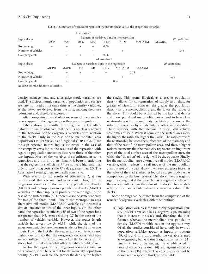
Table 7 shows the results of the regressions. For Alter-native 1, it can be observed that there is no clear tendencyin the behavior of the exogenous variables with relationto the slacks. Only in the case of the metropolitan areapopulation (MAP) variable and regional GDP (RGDP) arethe sign repeated in two inputs. However, in the case ofthe company costs input, the results of the regression withregard to population are contradictory to those of the othertwo inputs. Most of the variables are significant in someregressions and not in others. Finally, it bears mentioningthat the regression coefficients R2 are not very high and thatonly for operating costs is the R2 value greater than 0.5. TheAlternative 1 results, then, are hardly conclusive.

With regard to the results of Alternative 2, it canbe observed that certain tendencies exist. Thus, for theexogenous variables of the main city population density(MCPD) and metropolitan area population density (MAPD)variables, the three inputs all produce the same sign. In thecase of the surface ratio (SR), there is also the same tendencyfor two of the three inputs. Finally, the Metropolitan areaalternative rail modes (MAARMs) variable also presents asimilar tendency in two of the three inputs. On the otherhand, the regression coefficients R2 of two of the regressionsare greater than 0.5, even reaching 0.7 in the case of thenumber of vehicles variable. However, the routes lengthvariable has a very low R2 (0.15), while the signs of theexogenous variables have the same tendency for the other twoinputs. Due to the fact that the regression coefficients are nothigher, one can say that the exogenous variables used hereare not sufficient to explain completely the behavior of theslacks, but it is unknown what other variables would do so.

As for the signs of the exogenous variables used inAlternative 2, it can be seen that for the main city populationdensity (MCPD) variable, the greater the density, the higher

the slacks. This seems illogical, as a greater populationdensity allows for concentration of supply and, thus, forgreater efficiency. In contrast, the greater the populationdensity in the metropolitan areas, the lower the values ofthe slacks. This could be explained by the fact that denserand more populated metropolitan areas tend to have closerelationships with the main city, facilitating the use of theurban bus services by inhabitants of other municipalities.These services, with the increase in users, can achieveeconomies of scale. When it comes to the surface area ratio,the higher the ratio, the higher the slacks. The ratio providesthe relationship between the surface area of the main city andthat of the rest of the metropolitan area, and thus, a higherratio value means that the main city represents an importantpart of the total surface area of the metropolitan area, forwhich the “direction” of the sign will be the opposite. Finally,for the metropolitan area alternative rail modes (MAARMs)variable, which reflects the rail modes of the metropolitanarea but not of the capital city, their very existence increasesthe value of the slacks, which is logical as these modes act ascompetitors to the bus services. The slacks have a negativesign, meaning that if the variable has a negative coefficient,the variable will increase the value of the slacks. The variableswith positive coefficients reduce the negative value of theslacks.

Some findings can be drawn from the comparison of theresults of exogenous variables with other authors.

(i) Population variables: the main city population den-sity (MCPD) variable has a negative sign, meaningthat it increases the slack and, therefore, the inef-ficiency, whereas the metropolitan area populationdensity (MAPD) variable acts in the opposite way.Of all the studies considered here, only in two dopopulation variables appear as inputs or outputs[39, 43], and in a third study, the variable is usedas exogenous, but without a significant result [32].Finally, in two other studies, the variable acted infavor of efficiency in one [44] and against efficiencyin the other [36]. Thus, clear conclusions cannot bedrawn with respect to this type of variable.


(ii) Surface area variables: none of the studies directlyused the main city (MCS) or metropolitan areasurface (MAP) variables. In other studies, theseappear as population density variables.

(iii) Variables similar to wealth variables (RGDP) andalternative modes (COP, MCARM, and MAARM) areonly employed by [36] and his study differs from thisone in that there they appear as insignificant.

(iv) In [32], a dummy owner variable is included whichis only valid if the business is private. This variableacts in favor of efficiency. In the regression of theroute length variable slacks in Alternative 2, the PRIVvariable represents this idea and acts in the same way.

Thus, after comparing various studies, it can be statedthat it is not possible to come to conclusions with respectto the exogenous variables in order to contextualize theefficiency of the sector. The results are not homogenous.

8. Conclusions

The purpose of this paper is to analyze the technical efficiencyof the main urban bus companies in Spain. In order to dothis, an SBM model has been used because it enables a moreadjusted calculation of efficiency, due to the presence of theslacks. In the end, the final model obtained for calculating theefficiency included one variable indicating transit supply, onerelated to infrastructure, and two of the classic variables fromthe Cobb-Douglas models (fleet size and operating costs).

The efficiency values fluctuate between 0.514 and 1.000.19 DMUs reach the maximum value (1.000), representing23.5% of all the DMUs analyzed. Half of the cities presentthe maximum efficiency in, at least, one year. In these citiesthe bus companies are of various sizes. The companies ofMadrid, Oviedo, Zaragoza, and La Coruna are efficient in themajority of the years, while the companies of Mallorca andPamplona are efficient only in one year.

From the analysis of the slacks, the results cannot betaken literally; instead, they serve to highlight tendencieswith regard to the inefficiency value compared with adetermined variable. That is the case of Murcia, which has75% of routes length slacks. It does not mean that this % ofthe lines is remaining, but it is clear that Murcia may have aproblem of design of the network. The same can be said forefficient companies: they do not have a perfect service, buttheir surpluses are not very high.

The use of the slacks to perform the regression of theexogenous variables enables one to easily and comfortablystudy the inefficiency produced by the operating conditions.Analyzing slack by slack, one can study in a disaggregated waythe inefficiency of each input value used. In this way one canact in an individualized way with regard to each productionfactor in order to improve efficiency.

As for the exogenous variables analyzed here, althoughsome of the socioeconomic variables appear in the regres-sions, their presence is not repeated through all the regres-sions performed and they do not, therefore, display anytendency. Additionally, the regression coefficients R2 of these

regressions are not high. The urban population variables areindeed repeated in the different regressions and, as with theirsigns, display tendencies. The regression coefficients R2 inthese cases show higher values and thus are more reliable.

With this methodology, it is possible to study theefficiency of each variable used as an input: the study ofthe slacks allows for an understanding of the over sizing orunder sizing that exists for each one of the inputs. Then, itis possible to make recommendations to the companies insuch a way that they improve their efficiency. The analysis ofthe exogenous variables also allows to understand part of theinefficiency, but in a way that companies cannot do so much,because they have no power to influence these variables.

References

[1] A. Aparicio, Informe 2002 del Observatorio de la MovilidadMetropolitana, Ministerio de Medio Ambiente y Ministerio deFomento, Madrid, Spain, 2004.

[2] A. Monzon, A. M. Pardeiro, and P. Perez, Informe 2003 delObservatorio de la Movilidad Metropolitana, Ministerio deMedio Ambiente, Madrid, Spain, 2005.

[3] A. Monzon, A. M. Pardeiro, and P. Perez, Informe 2004 delObservatorio de la Movilidad Metropolitana, Ministerio deMedio Ambiente y Ministerio de Fomento, Madrid, Spain,2006.

[4] A. Monzon, R. Cascajo, A. M. Pardeiro, P. Jorda, P. Perez, andM. A. Delgado, Informe 2005 del Observatorio de la MovilidadMetropolitana, Ministerio de Medio Ambiente y Ministerio deFomento, Madrid, Spain, 2007.

[5] A. Monzon, R. Cascajo, P. Jorda, P. Perez, and I. Rojo,Informe 2006 del Observatorio de la Movilidad Metropolitana,Ministerio de Medio Ambiente y Medio Rural y Marino yMinisterio de Fomento, Madrid, Spain, 2008.

[6] A. Monzon, R. Cascajo, P. Jorda, P. Perez, M. Fernandez, andJ. del Alamo, Informe 2007 del Observatorio de la MovilidadMetropolitana, Ministerio de Medio Ambiente y Medio Ruraly Marino y Ministerio de Fomento, Madrid, Spain, 2009.

[7] A. Monzon, R. Cascajo, and P. Jorda, Informe 2008 delObservatorio de la Movilidad Metropolitana, Ministerio deMedio Ambiente y Medio Rural y Marino y Ministerio deFomento, Madrid, Spain, 2010.

[8] A. Monzon, R. Cascajo, P. Jorda, B. Munoz, and L. Delgado,Informe 2009 del Observatorio de la Movilidad Metropolitana,Ministerio de Medio Ambiente y Medio Rural y Marino yMinisterio de Fomento, Madrid, Spain, 2011.

[9] P. Jorda, Metodologıa de evaluacion de la eficiencia de losservicios de autobus urbano. Aplicacion a las grandes ciudadesespanolas en el periodo 2004–2009, Tesis doctoral, Departa-mento de Ingenierıa Civil: Transporte, Universidad Politecnicade Madrid, Madrid, Spain, 2012.

[10] B. De Borger, K. Kerstens, and A. Costas, “Public transitperformance: what does one learn from frontier studies?”Transport Reviews, vol. 22, no. 1, pp. 1–38, 2002.

[11] J. Odeck and A. Alkadi, “Evaluating efficiency in the Norwe-gian bus industry using data envelopment analysis,” Trans-portation, vol. 28, no. 3, pp. 211–232, 2001.

[12] N. K. Avkiran and T. Rowlands, “How to better identify thetrue managerial performance: state of the art using DEA,”Omega, vol. 36, no. 2, pp. 317–324, 2008.

[13] C. Pestana and N. Peypoch, “Productivity changes in Por-tuguese bus companies,” Transport Policy, vol. 17, no. 5, pp.295–302, 2010.


[14] A. Charnes, W. W. Cooper, and E. Rhodes, “Measuring theefficiency of decision making units,” European Journal ofOperational Research, vol. 2, no. 6, pp. 429–444, 1978.

[15] R. D. Banker, A. Charnes, and W. W. Cooper, “Somemodels for estimating technical and scale inefficiencies in dataenvelopment analysis,” Management Science, vol. 30, no. 9, pp.1078–1092, 1984.

[16] W. W. Cooper, L. M. Seiford, K. Tone, and J. Zhu, “Somemodels and measures for evaluating performances withDEA: past accomplishments and future prospects,” Journal ofProductivity Analysis, vol. 28, no. 3, pp. 151–163, 2007.

[17] L. R. Murillo-Zamorano, “Economic efficiency and frontiertechniques,” Journal of Economic Surveys, vol. 18, no. 1, pp. 33–45, 2004.

[18] K. Tone, “Slacks-based measure of efficiency in data envelop-ment analysis,” European Journal of Operational Research, vol.130, no. 3, pp. 498–509, 2001.

[19] H. O. Fried, S. S. Schmidt, and S. Yaisawarng, “Incorporatingthe operating environment into a nonparametric measure oftechnical efficiency,” Journal of Productivity Analysis, vol. 12,no. 3, pp. 249–267, 1999.

[20] P. Bogetoft and J. L. Hougaard, “Efficiency Evaluations Basedon Potential (Non-Proportional) Improvements,” Journal ofProductivity Analysis, vol. 12, no. 3, pp. 233–247, 1999.

[21] K. Tone, “A slacks-based measure of super-efficiency indata envelopment analysis,” European Journal of OperationalResearch, vol. 143, no. 1, pp. 32–41, 2002.

[22] H. Morita, K. Hirokawa, and J. Zhu, “A slack-based measureof efficiency in context-dependent data envelopment analysis,”Omega, vol. 33, no. 4, pp. 357–362, 2005.

[23] J. Liu and K. Tone, “A multistage method to measure efficiencyand its application to Japanese banking industry,” Socio-Economic Planning Sciences, vol. 42, no. 2, pp. 75–91, 2008.

[24] N. K. Avkiran, “Removing the impact of environment withunits-invariant efficient frontier analysis: an illustrative casestudy with intertemporal panel data,” Omega, vol. 37, no. 3,pp. 535–544, 2009.

[25] J. Zhu, “Super-efficiency and DEA sensitivity analysis,” Euro-pean Journal of Operational Research, vol. 129, no. 2, pp. 443–455, 2001.

[26] M. L. Delgado, M. A. Sanchez, and L. Mora, Reflexiones sobrela organizacion del transporte urbano colectivo en las grandesciudades, Catedra de Ecotransporte, Tecnologıa y Movilidad,Universidad Rey Juan Carlos, Madrid, Spain, 2009.

[27] CEOE, Memorandum: El sector del transporte en Espana,Confederacion Espanola de Organizaciones Empresariales,Madrid, Spain, 2009.

[28] G. Cheng and Z. Qian, “MaxDEA 5.0.,” 2011, http://www.maxdea.cn.

[29] J. F. Nolan, “Determinants of productive efficiency in urbantransit,” Logistics and Transportation Review, vol. 32, no. 3, pp.319–342, 1996.

[30] P. A. Viton, “Technical efficiency in multi-mode bus transit: aproduction fronteir analysis,” Transportation Research B, vol.31, no. 1, pp. 23–39, 1997.

[31] J. Cowie, “The technical efficiency of public and privateownership in the rail industry: the case of Swiss privaterailways,” Journal of Transport Economics and Policy, vol. 33,no. 3, pp. 241–252, 1999.

[32] K. Kerstens, “Technical efficiency measurement and expla-nation of french urban transit companies,” TransportationResearch A, vol. 30, no. 6, pp. 431–452, 1996.

[33] M. G. Karlaftis, “A DEA approach for evaluating the efficiencyand effectiveness of urban transit systems,” European Journalof Operational Research, vol. 152, no. 2, pp. 354–364, 2004.

[34] P. A. Viton, “Changes in multi-mode bus transit efficiency,1988–1992,” Transportation, vol. 25, no. 1, pp. 1–21, 1998.

[35] K. Kerstens, “Decomposing technical efficiency and effective-ness of French urban transport,” Annales d’economie et destatistique, vol. 54, pp. 129–155, 1999.

[36] I. M. Garcıa-Sanchez, “Technical and scale efficiency inSpanish urban transport: estimating with data envelopmentanalysis,” Advances in Operations Research, vol. 2009, ArticleID 721279, 15 pages, 2009.

[37] C. W. Cobb and P. H. Douglas, “A theory of production,” TheAmerican Economic Review, vol. 18, no. 1, pp. 139–165, 1928.

[38] P. Cantos, J. M. Pastor, and L. Serrano, “Productivity, efficiencyand technical change in the European railways: a non-parametric approach,” Transportation, vol. 26, no. 4, pp. 337–357, 1999.

[39] A. Novaes, “Rapid transit efficiency analysis with theassurance-region DEA method,” Pesquisa Operacional, vol. 21,no. 2, pp. 179–197, 2001.

[40] M. Asmild, T. Holvad, J. L. Hougaard, and D. Kronborg,“Railway reforms: do they influence operating efficiency?”Transportation, vol. 36, no. 5, pp. 617–638, 2009.

[41] J. F. Nolan, P. C. Ritchie, and J. E. Rowcroft, “Identifying andmeasuring public policy goals: ISTEA and the US bus transitindustry,” Journal of Economic Behavior and Organization, vol.48, no. 2, pp. 291–304, 2002.

[42] T. Holvad, J. L. Hougaard, D. Kronborg, and H. K. Kvist,“Measuring inefficiency in the Norwegian bus industry usingmulti-directional efficiency analysis,” Transportation, vol. 31,no. 3, pp. 349–369, 2004.

[43] V. Pina and L. Torres, “Analysis of the efficiency of localgovernment services delivery. An application to urban publictransport,” Transportation Research A, vol. 35, no. 10, pp. 929–944, 2001.

[44] D. T. Barnum, S. Tandon, and S. McNeil, “Comparing theperformance of bus routes after adjusting for the environmentusing data envelopment analysis,” Journal of TransportationEngineering, vol. 134, no. 2, pp. 77–85, 2008.

Documents

Analysis of the Technical Efficiency of Urban Bus Services in Spain Based on SBM Models