Seediscussions,stats,andauthorprofilesforthispublicationat:https://www.researchgate.net/publication/258640854

AnalysisofThermalProcessingofTableOlivesUsingComputationalFluidDynamics

ARTICLEinJOURNALOFFOODSCIENCE·NOVEMBER2013

ImpactFactor:1.7·DOI:10.1111/1750-3841.12277·Source:PubMed

CITATIONS

4

READS

66

4AUTHORS:

AdreasDimou

AgriculturalUniversityofAthens

9PUBLICATIONS58CITATIONS

SEEPROFILE

EfstathiosPanagou

AgriculturalUniversityofAthens

110PUBLICATIONS1,541CITATIONS

SEEPROFILE

NikolaosStoforos

AgriculturalUniversityofAthens

50PUBLICATIONS599CITATIONS

SEEPROFILE

StavrosYanniotis

AgriculturalUniversityofAthens

101PUBLICATIONS674CITATIONS

SEEPROFILE

Allin-textreferencesunderlinedinbluearelinkedtopublicationsonResearchGate,

lettingyouaccessandreadthemimmediately.

Availablefrom:EfstathiosPanagou

Retrievedon:04February2016

E:Fo

odEn

ginee

ring&

Phys

icalP

ropert

ies

Analysis of Thermal Processing of Table OlivesUsing Computational Fluid DynamicsA. Dimou, E. Panagou, N. G. Stoforos, and S. Yanniotis

Abstract: In the present work, the thermal processing of table olives in brine in a stationary metal can was studiedthrough computational fluid dynamics (CFD). The flow patterns of the brine and the temperature evolution in the olivesand brine during the heating and the cooling cycles of the process were calculated using the CFD code. Experimentaltemperature measurements at 3 points (2 inside model olive particles and 1 at a point in the brine) in a can (withdimensions of 75 mm × 105 mm) filled with 48 olives in 4% (w/v) brine, initially held at 20 ◦C, heated in waterat 100 ◦C for 10 min, and thereafter cooled in water at about 20 ◦C for 10 min, validated model predictions. Thedistribution of temperature and F-values and the location of the slowest heating zone and the critical point within theproduct, as far as microbial destruction is concerned, were assessed for several cases. For the cases studied, the criticalpoint was located at the interior of the olives at the 2nd, or between the 1st and the 2nd olive row from the bottom ofthe container, the exact location being affected by olive size, olive arrangement, and geometry of the container.

Keywords: computational fluid dynamics, critical point, heat transfer, table olives, thermal processing

Practical Application: The resulting knowledge from the present paper will help in thermal process optimization oftable olives which will lead to the production of safe and high-quality product with reduced salt content. In the presentpaper, only the safety issue, through the determination of the location of the critical point, as far as microbial destructionis concerned, was addressed.

IntroductionAccording to the Intl. Olive Council (IOC 2004) “Table Olives”

is the product prepared from the fruits of the cultivated olive tree(Olea europea L.) “treated to remove its bitterness and preservedby natural fermentation, or by heat treatment, with or withoutthe addition of preservatives,” packed with or without coveringliquid, and offered for trade and for final consumption. Basedon the preparation process the table olives have been undergone,IOC (2004) categorizes them in the following 5 trade preparations:treated olives, natural olives, dehydrated and/or shriveled olives,olives darkened by oxidation, and specialties.

The NaCl concentration, maximum pH, and minimum lacticacidity of the packing liquid, different for each trade preparation,dictate the severity of the heat treatment required for each typeof heat treated olives. Thus, for example, for all types of pasteur-ized olives a minimum of 2% NaCl brine can be used as longas pH does not exceed 4.3. On the same line, for commercialheat sterilized olives there is no minimum NaCl content, as longas maximum pH limit is set at 8.0 (Codex Alimentarius 1987).In a processing/preparation scheme in Greece for natural blackKalamata olives, with 2-y shelf life, aiming in product with re-duced salt content, the olives, after fermentation, are randomlypacked in jars or cans which are then filled with warm (65 ◦C)brine (4% NaCl with pH 3.4 to 3.8). The jars are sealed undervacuum and heat treated for 15 to 20 min in hot water of 80 ◦C,before cooling with 30 ◦C water.

MS 20130406 Submitted 3/21/2013, Accepted 8/26/2013. Authors are withDept. of Food Science and Human Nutrition, Agricultural Univ. of Athens, Athens,Greece. Direct inquiries to author Yanniotis (E-mail: yanniotis@aua.gr).

Different process schedules for whole ripe olives, with or with-out pits are suggested in Lopez (1987). The Intl. Olive Councilpublished minimum required F process values for thermal pro-cessing of different types of olives (IOC 2004). The F z

T value of athermal process (or simply F) is defined as the time in minutes ata constant temperature, T, required to destroy a given percentageof microorganisms whose thermal resistance is characterized byz, or, as the equivalent processing time of a hypothetical thermalprocess at a constant temperature that produces the same effect (interms of spore destruction) as the actual thermal process.

Thus, for olives using heat treatment as an added hurdle toattain microbial stability, a pasteurization process with an equiv-alent F 5.25◦C

62.4◦C value of at least 15 min is suggested. The aboverequired F process value, termed by IOC (2004) as pasteuriza-tion units (PU 5.25◦C

62.4◦C ), refers to propionic bacteria, characterizedby a z-value of 5.25 ◦C, as the reference microorganisms. Thereference temperature used, equal to 62.4 ◦C, is indicative of themild nature of the required thermal process. On the other hand,for those products exclusively relying on heat treatment for theirpreservation (as for olives darkened by oxidation) a severe thermalprocess, as those processes designed for commercial sterilizationof low acid foods, equivalent to a minimum Fo value of 15 min,is recommended (IOC 2004), where Fo value refers to a z-valueof 10 ◦C and a reference temperature of 121.11 ◦C (that is, Fo =F 10◦C

121.11◦C). Process schedules, that is heating time–retort tempera-ture combinations, to achieve the recommended F-values are leftto olive processors.

Referring to the IOC (2004) F-value suggestions, a vaguenessconcerning the location inside the container where the F-valuesshould be measured or calculated emerges. Are these F-values forthe covering (liquid) brine or the (solid) olives? If we quickly dis-regard the brine case, which olive becomes the critical particulate

C© 2013 Institute of Food Technologists R©

doi: 10.1111/1750-3841.12277 Vol. 78, Nr. 11, 2013 � Journal of Food Science E1695Further reproduction without permission is prohibited

E:FoodEngineering&PhysicalProperties

Analysis of olive thermal processing . . .

that we must monitor? Which region, within the critical olive(s),represents the “critical point,” that is the region inside the con-tainer that receives the least effect, in terms of destruction of theundesirable, target microorganisms, of the heat treatment? Knowl-edge of the heat transfer phenomena coupled with the appropriatemicrobial heat destruction kinetics is essential for answering theabove raised questions.

Computational fluid dynamics (CFD) has been used with in-creasing rate in food engineering research, in particular during thelast decade (Norton and Sun 2007). Problems dealing with thermalprocessing of liquid or liquid/particulate systems have been suc-cessfully approached through CFD, in terms of predicting transientvelocity and temperature profiles inside still processed containers.Examples include analysis of natural convection heating and bac-terial destruction in canned liquids (sodium carboxy-methyl cel-lulose [CMC] and water; Abdul Ghani and others 1999a, 1999b),heat transfer coefficient determination during natural convectionheating of CMC solutions in cylindrical containers (Kannan andGourisankar Sandaka 2008), pasteurization of beer (Augusto andothers 2010) or milk (Anand Paul and others 2011), and simula-tion of liquid/particulate thermal processing, such as large foodparticle in water (Rabiey and others 2007), pineapple slices injuice (Abdul Ghani and Farid 2006), peas in water (Kiziltas andothers 2010), and asparagus in brine (Dimou and Yanniotis 2011).

Quality degradation during thermal processing, for example,undesirable softening of the olive tissue, must be kept minimum.Thus, precise design and monitoring of the applied process is es-sential. The objective of the present work was to study the fluidflow and heat transfer phenomena during thermal processing oftable olives through CFD. In particular, fluid flow field, temper-ature evolution, distribution of F-values, and the location of thecritical point within the product, as far as microbial destructionis concerned, were assessed for several cases. The effect of thesize/shape of the olives in the performance of the process was alsoinvestigated.

Materials and Methods

Process detailsIn all simulated cases, a uniform initial temperature of 20 ◦C for

both olives and brine was used. Calculations were performed for10 min heating at 70 ◦C and 10 min cooling at 20 ◦C. This doesnot exactly correspond to a commercial process where the can isusually filled with hot brine (for example, 65 ◦C).

Three table olive geometries, differing in size or shape, wereconsidered. Thus we used 2 different size Kalamata olives (one25 mm long and 12 mm in diameter, termed hereafter “small” andanother 30 mm long and 19 mm in diameter, termed hereafter“large”) and a Conservolea one (30 mm long and 24 mm indiameter). All were designed as close as possible to their naturalshape (Figure 1).

For every case, a tin can with dimensions of 75 mm × 105 mmfilled with brine and the appropriate number of olives, necessary tofill up the container, was used. Eighty small-size Kalamata olives,in 8 rows with 10 olives per row, were orderly placed in the can(8×10 arrangement). Similarly, 48 large-size Kalamata olives (6×8arrangement) and 48 Conservolea olives (6×8 arrangement) werearranged in the can as presented in Figure 2. The above numberof olives approximately represents commercial practices for thecan size used. In addition to the 3-dimensional olive arrangement,vertical cross-sections for projection of data in 2-dimensional formare shown in Figure 2, for all cases studied.

Computational and theoretical modelThe system under investigation consisted of a stationary cylin-

drical metal can (75 mm in diameter, 105 mm in height) filledwith solid particles (table olives) and a covering liquid (brine) ini-tially at rest and at uniform temperature, heated at a medium withconstant temperature for a predescribed period of time followedby cooling at (also) constant medium temperature. We furtherconsidered infinite heat transfer coefficient between heating orcooling medium and external can wall, negligible resistance toheat transfer of the metal wall, and no slip at the container’s wall.Mass transfer from or to olives was neglected. Only heat trans-fer from the can to the brine and from the brine to olives wasconsidered.

Temperature evolution and flow patterns during natural con-vection heating for the system under investigation were calculatedby solving the governing partial differential equations for mass,momentum, and energy conservation (Bird and others 1960) withthe above-mentioned initial and boundary conditions. Since ananalytical solution to those equations is not feasible, they weresolved numerically as a system of algebraic equations applied infinite volumes that the system was discretized.

Software detailsThe software FLUENT 6.3.26, 2006 C© with 3D, double preci-

sion, pressure-based, laminar flow was used to solve the systemof partial differential equations. The use of laminar flow in themodel was justified since the Rayleigh nr (based on the length ofthe olive) was less than 107 during the heating and cooling cycle.A personal computer with IntelR© Core TM 2, CPU 660 @ 2.40GHz, 2048 MB RAM and Microsoft Windows XP ProfessionalR©

Version 2002 Service Pack 2 operating system was employed. Apreset convergence limit of 1×10−3 for continuity and momentumequations and 1×10−6 for the energy equation was used. The timestep used was equal to 0.5 s, the Courant nr was equal to 0.5, thealgorithm of pressure–velocity coupling was “Coupled,” and themodel used for the discretization of pressure was “PRESTO!”. Forthe discretization of momentum and energy equations, the model“Second Order Upwind” was selected.

In FLUENT nomenclature, the internal surface of the can, aswell as the external surface of the olives, was defined as wall. Thevolume of the olives was considered as solid .The volume betweenthe olives and the can, occupied by the brine, was considered asfluid. The volumes of the brine and the olives were designed inGambitR© 2.3.16.

The shape of the grid was “Tet/Hybrid – TGrid” for both olivesand brine volumes with the option of 10% “Shortest edge” of thesoftware. In this case of small Kalamata olives, 180982 cells in total(for both olives and brine) were used for the descretization andsolution of the governing equations, while for the large Kalamataand the Conservolea olives 130226 and 158559 cells, respectively,were employed. The above scheme was considered adequate, sincea finer grid, with about double the cells just mentioned for eachcase, that was also tested produced similar results. For such calcula-tions, the computational time was about 5, 2, and 3 d, for the caseof the small Kalamata, the large Kalamata, and the Conservoleaolives, respectively.

Physical propertiesKnowledge of the thermal and rheological properties of the

brine, as well as their temperature dependence, is essential in de-scribing the motion of the brine and consequently the rate of tem-perature rise during the thermal processing. The thermophysical

E1696 Journal of Food Science � Vol. 78, Nr. 11, 2013

E:Fo

odEn

ginee

ring&

Phys

icalP

ropert

ies

Analysis of olive thermal processing . . .

properties of 4% (w/v) NaCl aqueous solution obtained fromliterature (Irvine 1998) were used for the brine. More specifi-cally, each property was expressed as a function of temperature (T,in ◦C) through a 2nd- or 3rd-order polynomial equation (derivedin MicrosoftR© Office Excel) based on the temperature dependencevalues, for that particular property, obtained from the literaturedatabase (Irvine 1998). Thus, for a temperature range of 10 ◦C to130 ◦C, the input equations to FLUENT for density (ρ), specificheat (cp), thermal conductivity (k), and viscosity (μ) for the brineare shown on Table 1.

Density, heat capacity, and thermal conductivity of olives weremeasured experimentally at 20 ◦C (at least 5 replicates). Themethod of water displacement was used to measure olive density.Heat capacity was measured by Differential Scanning Calorimetry(model Q100, TA Instruments, Inc., New Castle, Del., U.S.A.)whereas the thermal conductivity was measured by a ThermalProperties Analyzer (model KD2, Decagon Devices Inc. Pullman,Wash., U.S.A.). The mean values shown on Table 1 for olives,that is constant values (temperature and variety independed), wereused as input data to FLUENT for all runs. The default FLUENTvalues for steel properties were used to describe the properties ofthe container.

Both flesh and kernel were treated as a whole with the samethermal properties. Preliminary runs were made using differentproperties between flesh and kernel. A thermal diffusivity valueequal to 0.8×10−7 m2/s (corresponding to low thermal diffusivity

Table 1–Physical and thermal properties of liquid and solids usedin simulationsa.

Brine(4% NaCl) Olive Teflon

ρ

(kg/m3)1.0334 × 103 − 2.0517 ×

10−1 × T − 2.4685 ×10−3 × T2

1035 ± 5 2240 ± 2.5

(R2 = 0.9999)μ

(Pa·s)1.7087 × 10−3 −

3.6550 × 10−5 × T +3.4048 × 10−7 × T2 −1.1334 × 10−9 × T3

– –

(R2 = 0.9981)Cp(J/kg·K)

3.9630 × 103 + 7.3626 ×10−2 × T + 5.3846 ×10−3 × T2

3200 ± 100 1050 ± 1

(R2 = 0.9999)k(W/m·K)

5.6592 × 10−1 +1.7906 × 10−3 × T −6.5734 × 10−6 × T2

0.40 ± 0.05 0.42 ± 0.001

(R2 = 0.9999)

aTemperature, T, in equations is in ◦C.

dry wood) was used for the kernel (compared to 1.2×10−7 m2/sdetermined and used for the flesh). Simulations show that forthe case where olive flesh and kernel were treated with the sameproperties (Case I) the product was heating and cooling slightly

Small Kalamata olives Large Kalamata olives Conservolea olives

Figure 1–Olive shape and dimensions used in simulations. (A) Small Kalamata olives, (B) large Kalamata olives, and (C) Conservolea olives.

A B CFigure 2–Three-dimensional arrangement of solidparticles (olives) in a vertical metal can and relatedvertical cross-sections for projection of data in2-dimensional form in subsequent figures. (A)Small-size Kalamata olives in 8 rows with 10 olivesper row (8×10 arrangement), (B) large-sizeKalamata olives (6×8 arrangement), and (C)Conservolea olives (6×8 arrangement).

Vol. 78, Nr. 11, 2013 � Journal of Food Science E1697

E:FoodEngineering&PhysicalProperties

Analysis of olive thermal processing . . .

faster compared to the case where different kernel properties (CaseII) were considered due to differences in thermal diffusivity values.Differences in temperatures between the 2 cases were rather small.For example, after 8 min of heating at 70 ◦C of a can with 48Conservolea olives, the temperature at the slowest heating point(SHP) for Case I was 64.1 ◦C and for Case II the correspondingvalue was 63.6 ◦C. Including cooling, the accumulated F-value atthe critical point for Case I was 5.2 min and for Case II 4.7 min.After 10 min of heating at 70 ◦C, the corresponding temperaturevalues were 66.9 ◦C and 66.6 ◦C, for Case I and II, respectively,

Figure 3–Comparisons between experimental (Exp I and Exp II) and sim-ulated (CFD) temperature data for large Kalamata olives (6×8 arrange-ment) in 4% (w/v) brine in a stationary metal can during heating andcooling in water. TW represents the internal can wall temperature. (A)Brine temperature at a point with x = 1.8 mm, y = –6.5 mm, and z = 0coordinates, (B) temperature at the center of an olive located in the middleof the 2nd row from the bottom (x = 6 mm, y = –2.9 mm, and z = 0 mm),and (C) temperature at the center of an olive located in the middle of the2nd row from the top (x = 0 mm, y = 16.6 mm, and z = –6 mm).

while the accumulated F-value at the critical point for Case I was19.4 min and for Case II 18.1 min. Due to the calculated smalltemperature differences between the 2 cases and the uncertaintiesin kernel properties (which by itself is not homogeneous) it wasdecided to not take into account any differences between flesh andkernel properties.

F-value calculationA User Defined Function (UDF) was written and imported to

FLUENT in order to calculate the F-value of the process throughEq. 1, based on the classical thermobacteriological approach (Balland Olson 1957).

F zTr e f

=∫ t

010

T−Tr e fz d t (1)

Equation 1 is based on 1st-order microbial reduction kinet-ics and linear dependency of the logarithm of decimal reductiontime on temperature. Although deviations from 1st-order kineticshave been observed and sophisticated models have been reportedin the literature (Sapru and others 1993), the 1st-order modelis generally accepted as an engineering tool for thermal processcalculations (Pflug 1987) and has a successful record of applica-tions in the thermal processing industry. It is worth to notice thatEq. 1 is also applicable for nth order reactions with any limita-tions originating from the definition of the z-value (Stoforos andothers 1997) although in these cases the F-value does not directlyrepresent logarithmic reduction of microbial population. As faras the temperature dependence of thermal destruction rates, forthe rather short range of temperatures, where inactivation takesplace, a number of models, including the z-value approach, areconsidered adequate.

F-values were calculated at every point inside the containerwhere temperature values were available, that is, at every node ofthe grid, through numerical integration of Eq. 1, using the trape-zoidal rule, based on a z-value of 5.25 ◦C (indicative to propi-onic bacteria) and a reference temperature of 62.4 ◦C, appropriatefor pasteurization processes. Thus, the distribution of the F-valuecould be assessed.

Model validationAn experimental procedure was employed in order to evaluate

the performance of the proposed model. For this, experimentaltemperature data for large Kalamata olives (6×8 arrangement) in4% (w/v) brine in a stationary metal can (with dimensions of75 mm × 105 mm) during heating and cooling in water werecollected at 3 points: (1) in a point in the brine, between the3rd and the 4th olive row, and specifically, at the point with x =18 mm, y = –6.5 mm, and z = 0 coordinates; (2) at the center ofa model olive located in the middle of the 2nd row from the canbottom (x = 6 mm, y = –29 mm, and z = 0 mm); and (3) at thecenter of a model olive located in the middle of the 2nd row fromthe top of the can (x = 0 mm, y = 16.6 mm, and z = –6 mm).The origin, x = 0, y = 0, and z = 0 is at the geometric centerof the can, x and y (which coincides with the axis of the cylinder)are at the plane of the paper, with positive x to the right andpositive y to the top, and positive z coming out of the plane of thepaper toward the reader as shown in Figure 2. The 46 out of the48 olives that the can was filled with during the validation exper-iments were actual Kalamata olives. The other 2 olives, for whichtemperature data were obtained, were model olives, made fromTeflon (glassy type, bought and handcrafted by a local supplier

E1698 Journal of Food Science � Vol. 78, Nr. 11, 2013

E:Fo

odEn

ginee

ring&

Phys

icalP

ropert

ies

Analysis of olive thermal processing . . .

with properties shown in Table 1). The substitution of 2 actualolives with model olives was necessary, since variation on olivesize and uncertainty on the precise location of the thermocou-ple inside the olive, that was tried initially, caused variations oncollected temperature data. Thus, 2 model Teflon olives, madeto similar shape and size as the actual olives, with thermocouplesfixed at their center, were used to collect temperature data dur-ing thermal processing. Temperature data were collected througha temperature recorder (OMEGA ENGINEERING, OM-220)with type K thermocouples 0.5 mm in diameter in replicate ex-periments. The can and its contents were initially held at 20 ◦C,and thereafter they were heated in water at about 100 ◦C for10 min and cooled in water at about 20 ◦C for 10 min. CFD sim-ulations of the above experimental setup were performed, withthe 2 Teflon model olives (and their properties) been used at theappropriate positions inside the can, instead of the actual Kalamataolives. This was done only in the validation runs.

Results and Discussion

Model validationFor the model validation trials, comparison between

experimentally determined temperatures and corresponding CFDpredicted values was satisfactory (Figure 3). Variation betweenreplicate experiments, as far as temperatures at the center of the(model) olives is concerned, was higher than the differences be-tween predicted and experimental values (Figure 3B and 3C).Differences between predicted and experimental values for thetemperature measurements in the brine were higher comparedto those in the Teflon olives; it is expected that such differencesattenuate as we proceed along the center of the olives.

Based on the observed agreement between experimental andpredicted data, the selected parameters and procedures for theCFD calculations through the FLUENT software were consideredappropriate and were retained in all subsequent runs. It is worthto say here, that early trial runs with different time steps (0.01,0.1, and 0.5 s) produced similar results (less than 0.5% momentarydifferences on temperature values and about 0.3% differences onF-values—data not shown) and therefore, the biggest time step of0.5 s, which considerably saved calculation time (45, 7, and 2 d

for time steps of 0.01, 0.1, and 0.5 s, respectively, for the case oflarge Kalamata olives), was used.

Velocity profileThe movement of the brine in the can was a typical, natural

convection, motion. During the heating cycle, the heated brinenear the wall is moving upward, toward the top of the containerdue to buoyancy forces, forcing the brine sitting on the top of thecontainer to move downward at the interior of the can throughthe layers of olives. This circular flow is repeated until the brineapproaches the temperature of the heating medium (approximatelyafter 7 min of heating, Figure 3A). The presence of the olivessubstantially affects the flow of the brine. Figure 4 shows such apattern after 30 s of heating for the different cases examined. Thesimulation of the flow field, as exported from the CFD model,is in agreement with literature results (Hiddink and others 1976;Datta and Teixeira 1988; Kumar and others 1990). Thirty secondsafter the onset of heating, maximum calculated velocities were2.627 cm/s, 2.619 cm/s, and 3.065 cm/s for the case of 4% brinefilled with small Kalamata, large Kalamata, and Conservolea olives,respectively.

When the cooling phase starts, the direction of brine movementis changing. Now the brine is moving downward near the wallbecause of the fluid’s cooling and upward in the interior can space.Thirty seconds after the onset of cooling, maximum calculatedvelocities were 2.558 cm/s, 2.113 cm/s, and 3.017 cm/s for thecase of 4% brine filled with small Kalamata, large Kalamata, andConservolea olives, respectively.

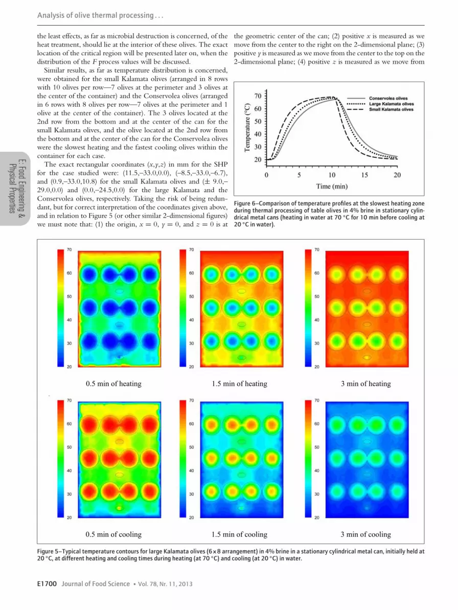
Temperature profileTypical temperature contours for large Kalamata olives (arranged

in 6 rows with 8 olives per row—6 olives at the perimeter and 2olives at the center of the container) in 4% brine at different heatingand cooling times are shown in Figure 5. The olives located at the2nd row from the bottom and at the center of the can were theslowest heating olives within the container. The interior of theseolives represented the slowest heating region of the system underinvestigation. Due to the brine motion, these same olives werethe fastest cooling olives during the cooling cycle of the process,as it is evident from Figure 5, after 3 min of cooling. Thus, thecritical region (or critical point), that is, the region that receives

Small Kalamata οlives Large Kalamata οlives Conservolea οlives

Figure 4– Velocity profiles of 4% brine (initially held at 20 ◦C) in a stationary cylindrical can filled with table olives after 30 s of heating at 70 ◦C(velocity in cm/s).

Vol. 78, Nr. 11, 2013 � Journal of Food Science E1699

E:FoodEngineering&PhysicalProperties

Analysis of olive thermal processing . . .

the least effects, as far as microbial destruction is concerned, of theheat treatment, should lie at the interior of these olives. The exactlocation of the critical region will be presented later on, when thedistribution of the F process values will be discussed.

Similar results, as far as temperature distribution is concerned,were obtained for the small Kalamata olives (arranged in 8 rowswith 10 olives per row—7 olives at the perimeter and 3 olives atthe center of the container) and the Conservolea olives (arrangedin 6 rows with 8 olives per row—7 olives at the perimeter and 1olive at the center of the container). The 3 olives located at the2nd row from the bottom and at the center of the can for thesmall Kalamata olives, and the olive located at the 2nd row fromthe bottom and at the center of the can for the Conservolea oliveswere the slowest heating and the fastest cooling olives within thecontainer for each case.

The exact rectangular coordinates (x,y,z) in mm for the SHPfor the case studied were: (11.5,–33.0,0.0), (–8.5,–33.0,–6.7),and (0.9,–33.0,10.8) for the small Kalamata olives and (± 9.0,–29.0,0.0) and (0.0,–24.5,0.0) for the large Kalamata and theConservolea olives, respectively. Taking the risk of being redun-dant, but for correct interpretation of the coordinates given above,and in relation to Figure 5 (or other similar 2-dimensional figures)we must note that: (1) the origin, x = 0, y = 0, and z = 0 is at

the geometric center of the can; (2) positive x is measured as wemove from the center to the right on the 2-dimensional plane; (3)positive y is measured as we move from the center to the top on the2-dimensional plane; (4) positive z is measured as we move from

Figure 6–Comparison of temperature profiles at the slowest heating zoneduring thermal processing of table olives in 4% brine in stationary cylin-drical metal cans (heating in water at 70 ◦C for 10 min before cooling at20 ◦C in water).

0.5 min of heating 1.5 min of heating 3 min of heating

0.5 min of cooling 1.5 min of cooling 3 min of cooling

Figure 5–Typical temperature contours for large Kalamata olives (6×8 arrangement) in 4% brine in a stationary cylindrical metal can, initially held at20 ◦C, at different heating and cooling times during heating (at 70 ◦C) and cooling (at 20 ◦C) in water.

E1700 Journal of Food Science � Vol. 78, Nr. 11, 2013

E:Fo

odEn

ginee

ring&

Phys

icalP

ropert

ies

Analysis of olive thermal processing . . .

the center out of the paper. Thus, the (0.0,–24.5,0.0) coordinatesgiven for the Conservolea olives locates the SHP at the center axis,28 mm from the bottom of the container. Also note that for thesmall Kalamata olives there are 3 positions (corresponding to the

interior of 3 olives) while for the large Kalamata olives 2 positionswhere the SHP is located.

The temperature profiles for the slowest heating zone during thethermal process for the cases studied are presented in Figure 6. For

Figure 7–F-value distribution within the olives at the end of a thermal process consisting of heating in water at 70 ◦C for 10 min before cooling in waterat 20 ◦C in a stationary cylindrical metal can.

Figure 8–Location of the critical point of a thermal process consisting of heating in water at 70 ◦C for 10 min before cooling in water at 20 ◦C in astationary cylindrical metal can. Illustration includes appropriate side (1st row) and top (2nd row) views at the planes where the olives containing thecritical point are located.

Vol. 78, Nr. 11, 2013 � Journal of Food Science E1701

E:FoodEngineering&PhysicalProperties

Analysis of olive thermal processing . . .

the conditions examined, the size of the olives was the determinedparameter on the temperature of the SHP.

F-value distributionThe distribution of the F 5.25◦C

62.4◦C process values for the olives ispresented in Figure 7. An extensive differentiation of F-values,based on olive size, location of the olives inside the container andthe point of interest inside the olive, is evident. For the thermaltreatments applied, process F-values ranged approximately from70 min (for the interior of the olives located at or close the SHP)to 160 min (at the surface of the olives located at the top of the can)for the case of small Kalamata olives. The corresponding rangesfor the large Kalamata and Conservolea olives were 37 min to130 min and 20 min to 145 min, respectively.

The point, the critical point, that should be monitored, in orderto assess the effectiveness of a given process, should be preciselyknown. At the end of the entire process, the exact coordinates(x,y,z) in mm, for the critical point for the cases studied were:(9.2,–33.0,–5.2), (–8.5,–33.0,–6.7), and (0.9,–33.0,10.8) for thesmall Kalamata olives and (± 7.0,–30.5,0.0) and (0.0,–35.0,0.0),for the large Kalamata and the Conservolea olives, respectively(Figure 8). Note that the critical points did not coincide with

the SHP, due to the lethal contribution of the cooling cycle.However, from a practical point of view it should be pointed outthat differences in F-values were not important with respect to thesafety precautions taken in designing thermal processes.

Due to the nonsymmetrical olive arrangement (Figure 2), the3 olives located at the 2nd row from the bottom and at the centerof the can, for the small Kalamata olives where the critical pointswere located (Figure 8A), did not exhibit exactly the same F-values. Specifically, the exact F 5.25◦C

62.4◦C values at the 3 critical pointsfor the small Kalamata olives were 64, 64.3, and 65.2 min. Thesevalues were notably different from the minimum F-values achievedat the 7 surrounding olives, ranging from 68.9 to 71.4 min, withthe olives on the bottom row having minimum F-values from73.2 min to 77.2 min, and the olives on the 3rd row from thebottom having minimum F-values from 70.2 to 77.6 min.

Similarly, for the large Kalamata olives, the exact F 5.25◦C62.4◦C values

at the 2 critical points were 38.8 and 39.0 min. The minimumF-values achieved at the 6 surrounding olives ranged from 47.8 to48.2 min, the olives on the bottom row having minimum F-valuesfrom 42 min (at the central axis) to 54 min (at the circumferenceof the can), and the olives on the 3rd row from the bottom havingminimum F-values from 47.5 to 57.8 min.

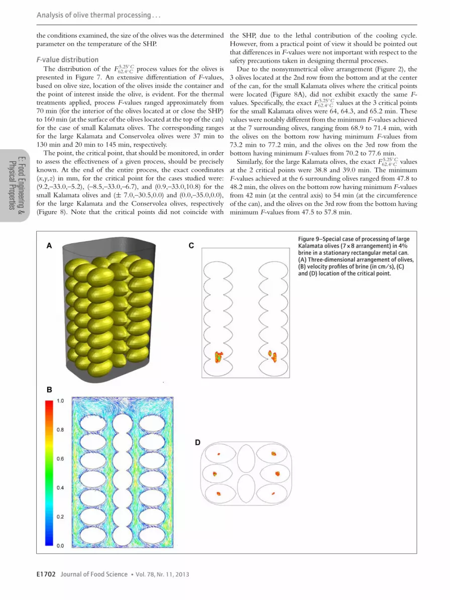
Figure 9–Special case of processing of largeKalamata olives (7×8 arrangement) in 4%brine in a stationary rectangular metal can.(A) Three-dimensional arrangement of olives,(B) velocity profiles of brine (in cm/s), (C)and (D) location of the critical point.

E1702 Journal of Food Science � Vol. 78, Nr. 11, 2013

E:Fo

odEn

ginee

ring&

Phys

icalP

ropert

ies

Analysis of olive thermal processing . . .

Finally, for the Conservolea olives, the exact F 5.25◦C62.4◦C value at the

critical point was 20.0 min. For this case, the Conservolea olivesat the central axis were slightly pressed one on top of the other,so that there was some overlapping between the volumes of the 2separate olives (Figure 7). The critical point was located betweenthe 2 central olives located at the last 2 rows (Figure 8C). Theminimum F-values achieved at the 2 olives, above and bellow thecritical point, were 21.0 and 21.5 min, respectively. The olives atthe circumference of the can at the bottom row had minimum F-values from 27.2 to 28.9 min, while the olives at the circumferenceof the can at the 2nd row from the bottom had minimum F-values32.6 min.

Based on the quantitative data presented in the previous para-graphs, the identification of the critical point as presented inFigure 8 is justified. Asymmetrical heating gives rise to slightdifferences on minimum F-values for the critical points presentedin Figure 8, but these points are clearly distinguished from thepoints with minimum F-values at the rest of the olives. In all casesstudied, the brine around the central axis and toward the bottomof the container represented the cold fluid volume of the system.Particle size (as it mainly influences heat flux by conduction) aswell as particle orientation, arrangement, and packing density (asit influences brine motion and therefore heat transfer from thebrine to the particles) will affect the exact location of the criticalpoint. Thus, for example, for some particular case, olives awayfrom the can central axis can contain the critical point. Such acase is illustrated in Figure 9.

Large Kalamata olives (arranged in 7 rows with 8 olives per row)in 4% brine are processed in a rectangular tin container (82 mmin length, 57 mm in width, and 121 mm in height) as shown inFigure 9A. The same time–temperature conditions, as for the casesin the cylindrical can presented so far, were applied. Comparedto the previous cases, fluid velocities were more uniform for thiscase and rather high between the olives located at the center of thecontainer, probably due to the availability of free space betweenthe olives (Figure 9B). As a result, the critical point was locatedat the interior of the olives located away from the central plane asillustrated in Figure 9C and 9D.

ConclusionsFluid flow and heat transfer phenomena during thermal process-

ing of table olives in brine, in a stationary tin can, were successfullysimulated through CFD. Consequently, the distribution of tem-perature and F-values and the location of the slowest heating zoneand the critical point within the product, as far as microbial de-struction is concerned, were assessed. For the cases studied, thecritical point was located at the interior of the olives at the 2nd, orbetween the 1st and the 2nd olive row from the bottom of the con-tainer. The critical points did not exactly coincide with the pointsof the slowest heating zone, due to the lethal contribution of thecooling cycle. A number of parameters need to be determined and

studied further, for example, the effect of olive placement (orderlyor randomly), container orientation (vertical or horizontal), andshape (cylindrical or rectangular), as they might affect the brineflow and the exact location of the critical point. In analogy tothe work presented in the current investigation, one can calculatequality degradation at the end of a thermal process given the keyquality parameter and the kinetics of its thermal degradation. Dif-ferent time–temperature schedules, leading to safe product, canbe evaluated in terms of their impact to product quality, throughan optimization scheme, and select the one that will lead to theproduction of safe product with the least quality degradation.

ReferencesAbdul Ghani AG, Farid MM. 2006. Using the computational fluid dynamics to analyze the

thermal sterilization of solid–liquid food mixture in cans. Innov Food Sci Emerg 7:55–61.Abdul Ghani AG, Farida MM, Chena XD, Richards P. 1999a. Numerical simulation of natural

convection heating of canned food by computational fluid dynamics. J Food Eng 41(1):55–64.Abdul Ghani AG, Farida MM, Chena XD, Richards P. 1999b. An investigation of deactivation

of bacteria in a canned liquid food during sterilization using computational fluid dynamics(CFD). J Food Eng 42(4):207–14.

Anand Paul D, Anishaparvin A, Ananndharamakrishnan C. 2011. Computational fluid dynamicsstudies on pasteurisation of canned milk. Int J Dairy Technol 64(2):305–13.

Augusto PED, Pinheiro TF, Marcelo Cristianini M. 2010. Using computational fluid-dynamics(CFD) for the evaluation of beer pasteurization: effect of orientation of cans. Cienc TecnolAliment Campinas 30(4):980–86.

Ball CO, Olson FCW. 1957. Sterilization in food technology. Theory, practice and calculations.New York: McGraw-Hill Book Co. p 654.

Bird RB, Stewart WE, Lightfoot EN. 1960. Transport phenomena. New York: John Wiley andSon. p 905.

Codex Alimentarius. 1987. Codex Standard for Table Olives, Codex Stan 66, Codex Ali-mentarius, International Food Standards. Available from: http://www.codexalimentarius.org/standards/list-of-standards/en/?no_cache=1. Accessed 2012 Oct 14.

Datta AK, Teixeira AA. 1988. Numerically predicted transient temperature and velocity profilesduring natural convection heating of canned liquid foods. J Food Sci 53(1):191–5.

Dimou A, Yanniotis S. 2011. 3-D numerical simulation of asparagus sterilization using compu-tational fluid dynamics. J Food Eng 104(3):394–403.

Hiddink J, Schenk J, Bruin S. 1976. Natural convection heating of liquids in closed containers.Appl Sci Res 32:217–37.

IOC (Intl. Olive Council). 2004. Trade Standard Applying to Table Olives, Resolution NrRES-2/91-IV/04, COI/OT/NC nr 1. Available from: http://www.internationaloliveoil.org.Accessed 2012 Oct 14.

Irvine TF Jr. 1998. Thermophysical properties. In: Rohsenow WM, Hartnett JR, Cho YI,editors. Handbook of heat transfer. 3th ed. New York: The McGraw-Hill Co., Inc. p 2.1–2.74.

Kannan A, Gourisankar Sandaka PCh. 2008. Heat transfer analysis of canned food sterilizationin a still retort. J Food Eng 88:213–28.

Kiziltas S, Erdogdu F, Palazoglu K. 2010. Simulation of heat transfer for solid–liquid foodmixtures in cans and model validation under pasteurization conditions. J Food Eng 97:449–56.

Kumar A, Bhattacharya M, Blaylock J. 1990. Numerical simulation of natural convection heatingof canned thick viscous liquid food products. J Food Sci 55(5):1403–11, 1420.

Lopez A. 1987. A complete course in canning and related processes. Book III, Processingprocedures for canned food products. 12th ed. Baltimore, Md.: The Canning Trade Inc. p516.

Norton T, Sun DW. 2007. An overview of CFD applications in the food industry. In: Sun DW,editor. Computational fluid dynamics in food processing. Boca Raton, Fla.: CRC Press. p1–41.

Pflug IJ. 1987. Using the straight-line semilogarithmic microbial destruction model as an engi-neering design model for determining the F-value for heat processes. J Food Prot 50(4):342–6.

Rabiey L, Flick D, Duquenoy A. 2007. 3D simulations of heat transfer and liquid flow duringsterilization of large particles in a cylindrical vertical can. J Food Eng 82:409–17.

Sapru V, Smerage GH, Teixeira AA, Lindsay JA. 1993. Comparison of predictive models forbacterial spore population resources to sterilization temperatures. J Food Sci 58(1):223–8.

Stoforos NG, Noronha J, Hendrickx M, Tobback P. 1997. A critical analysis of mathematicalprocedures for the evaluation and design of in-container thermal processes of foods. Crit RevFood Sci Nutr 37(5):411–41.

Vol. 78, Nr. 11, 2013 � Journal of Food Science E1703