Analyzing uncertainties of probabilistic rough set regions with game-theoretic rough sets

International Journal of Approximate Reasoning 55 (2014) 142–155

Contents lists available at SciVerse ScienceDirect

International Journal of Approximate Reasoning

j o u r n a l h o m e p a g e : w w w . e l s e v i e r . c o m / l o c a t e / i j a r

Analyzing uncertainties of probabilistic rough set regions with

game-theoretic rough sets

Nouman Azam, JingTao Yao ∗

Department of Computer Science, University of Regina, Regina, Canada SK S4S 0A2

A R T I C L E I N F O A B S T R A C T

Article history:

Available online 13 April 2013

Keywords:

Game-theoretic rough sets

Probabilistic rough sets

Uncertainty

Probabilistic rough set approach defines the positive, negative and boundary regions, each

associated with a certain level of uncertainty. A pair of threshold values determines the

uncertainty levels in these regions. A critical issue in the community is the determination

of optimal values of these thresholds. This problem may be investigated by considering a

possible relationship between changes in probabilistic thresholds and their impacts on

uncertainty levels of different regions. We investigate the use of game-theoretic rough

set (GTRS) model in exploring such a relationship. A threshold configuration mechanism

is defined with the GTRS model in order to minimize the overall uncertainty level of rough

set based classification. By realizing probabilistic regions as players in a game, a mechanism

is introduced that repeatedly tunes the parameters in order to calculate effective threshold

parameter values. Experimental results on text categorization suggest that the overall uncer-

tainty of probabilistic regionsmay be reducedwith the threshold configurationmechanism.

© 2013 Elsevier Inc. All rights reserved.

1. Introduction

Probabilistic rough sets [37] extended the Pawlak [25] rough setmodel by considering probabilistic information of objects

being in a set for determining their inclusion in the positive, negative or boundary regions. The divisions among these three

regions are defined by a pair of threshold values. Although the Pawlak positive and negative regions provide aminimum level

of classification errors, they are often applicable to a few objects [5,7]. This limits the practical applicability of the theory in

real world applications [31,37]. Probabilistic rough sets expanded the rough sets applicability or generality by incorporating

more objects in positive and negative regions at a cost of some classification errors (which reduces the accuracy) [35,34]. A

pair of thresholds controls the level of tradeoff between the properties of generality and accuracy. The determination and

interpretation of thresholds are fundamental issues in probabilistic rough sets [40].

The decision-theoretic rough set (DTRS) model calculates the probabilistic thresholds by utilizing different cost func-

tions to minimize the overall risk or cost in classifying objects [42]. An optimization viewpoint of DTRS was proposed for

automatically learning the required thresholds from data [15,16]. Other attempts for calculating thresholds in the DTRS

framework include a multi-view decision model [19], and a four level approach that puts additional conditions at each

successive level, thereby restricting or limiting the domains of thresholds [22]. Some recent studies on DTRS may be found

in references [20,21,27,32]. The game-theoretic rough set (GTRS) model was introduced for calculating the required thresh-

olds within a game-theoretic learning environment [13]. The configuration of probabilistic thresholds is interpreted as a

decision making problem in a competitive game involving multiple criteria [5]. The importance of GTRS is that it enables a

tradeoff mechanism through simultaneous consideration of multiple properties or aspects for an effective determination of

thresholds.

∗ Corresponding author.

E-mail addresses: [email protected] (N. Azam), [email protected] (J.T. Yao).

0888-613X/$ - see front matter © 2013 Elsevier Inc. All rights reserved.

http://dx.doi.org/10.1016/j.ijar.2013.03.015

http://crossmark.crossref.org/dialog/?doi=10.1016/j.ijar.2013.03.015&domain=pdf


http://www.sciencedirect.com/science/journal/0888613X

www.elsevier.com/locate/ijar


N. Azam, J.T. Yao / International Journal of Approximate Reasoning 55 (2014) 142–155 143

Deng and Yao [7] recently proposed an information-theoretic interpretation of probabilistic thresholds. The uncertainties

with respect to different regions were calculated by utilizing the measure of Shannon entropy. By providing the notion of

overall uncertainty calculated as an average uncertainty of the three regions, the formulation provides another motivation

for studying the probabilistic rough sets. The Pawlak positive and negative regions have a minimum uncertainty of zero,

however it may not have the minimum overall uncertainty due to large size of the boundary region [7]. Another extreme

case is considered in the form of probabilistic two-way decision model which as opposed to Pawlak model has a minimum

size boundary region. Although the uncertainty of the boundary region is minimum in this case, the overall uncertainty

may not be necessarily minimum for themodel. The probabilistic rough set model is utilized to consider the tradeoff among

uncertainties of the three regions through suitable adjustments in threshold values [7].

The problem of finding an effective threshold pair was formulated as a minimization of uncertainty of three-way classi-

fication induced by the three regions in [7]. However, an explicit mechanism for searching or learning an optimal threshold

pair in the space of possible threshold pairs was not provided. A GTRS based approach may be considered to address this

issue.

We use the GTRS model to construct a mechanism for analyzing the uncertainties of rough set regions in the aim of

finding effective threshold values. A competitive game is formulated between the regions that modify the thresholds in

order to improve their respective uncertainty levels. By repeatedly playing the game and utilizing its results for updating

the thresholds, a learning mechanism is proposed that automatically tunes the thresholds based on the data itself.

2. Uncertainties in probabilistic rough set regions

We briefly review the main results of probabilistic rough sets [37,40] in this section.

Suppose U is a finite set of objects called universe and E ⊆ U × U is an equivalence relation on U. An equivalence

class of E which contains an object x ∈ U is given by [x]E (or for simplicity by [x]). The set of all equivalence classes, i.e.

U/E = {[x]|x ∈ U}, provides a partition of U. For a particular C ⊆ U containing instances of a concept, P(C|[x]) denotes theconditional probability of an object in C given that the object is in [x]. The lower and upper approximations of a concept C

are defined by using a threshold pair (α, β) (with 0 ≤ β < α ≤ 1) as follows.

apr(α,β)

(C) = ⋃{[x] ∈ U/E | P(C|[x]) ≥ α},apr(α,β)(C) = ⋃{[x] ∈ U/E | P(C|[x]) > β}. (1)

The (α, β)-probabilistic positive, negative and boundary regions can be defined based on (α, β)-lower and upper

approximations, which are also named as probabilistic three-way decision model [39,41]:

POS(α,β)(C) = apr(α,β)

(C)

= {x ∈ U|P(C|[x]) ≥ α},NEG(α,β)(C) = (apr(α,β)(C))c

= {x ∈ U|P(C|[x]) ≤ β},BND(α,β)(C) = (POS(α,β)(C) ∪ NEG(α,β)(C))c

= {x ∈ U|β < P(C|[x]) < α}. (2)

The conditional probability may be recognized as a level of confidence that an object having the same description as x

belongs to C. For an object y having the same description as x, we accept it to be in C if the confidence level is greater than or

equal to levelα, i.e. P(C|[x]) ≥ α. The same object ymay be rejected to be in C if the confidence level is lesser than or equal to

level β , i.e. P(C|[x]) ≤ β . The decision about object y to be in C may be deferred if the confidence is between the two levels,

i.e. β < P(C|[x]) < α. Other rough set models may be obtained by setting special conditions on (α, β) threshold pair. For

instance, we obtain the Pawlak rough set model when we set (α, β) = (1, 0). A probabilistic two-way decision model may

be obtained with α = β . Moreover, a special 0.5 probabilistic rough set model may be obtained with α = β = 0.5 [36].

2.1. An information-theoretic interpretation of probabilistic rough sets

The information-theoretic interpretation of probabilistic rough sets was formulated in [7]. Considering a pair of prob-

abilistic thresholds that is used to generate three disjoint regions corresponding to a concept C, i.e. positive, negative and

boundary regions. A partition with respect to the probabilistic thresholds (α, β) can be formed as [7],

π(α,β) = {POS(α,β)(C),NEG(α,β)(C), BND(α,β)(C)}. (3)

144 N. Azam, J.T. Yao / International Journal of Approximate Reasoning 55 (2014) 142–155

Another partition with respect to a concept C can be formed as πC = {C, Cc}. The uncertainty in πC with respect to the

three probabilistic regions may be computed with Shannon entropy as follows [7]:

H(πC |POS(α,β)(C)) = −P(C|POS(α,β)(C)) log P(C|POS(α,β)(C))

−P(Cc|POS(α,β)(C)) log P(Cc|POS(α,β)(C)),

H(πC |NEG(α,β)(C)) = −P(C|NEG(α,β)(C)) log P(C|NEG(α,β)(C))

−P(Cc|NEG(α,β)(C)) log P(Cc|NEG(α,β)(C)),

H(πC |BND(α,β)(C)) = −P(C|BND(α,β)(C)) log P(C|BND(α,β)(C))

−P(Cc|BND(α,β)(C)) log P(Cc|BND(α,β)(C)). (4)

The above three equations may be viewed as the measure of uncertainty in πC with respect to POS(α,β)(C), NEG(α,β)(C)and BND(α,β)(C) regions. The conditional probabilities in these equations, e.g. P(C|POS(α,β)(C)) may be interpreted as the

probability of C given the knowledge of POS(α,β)(C). The conditional probabilities for the positive region are computed as,

P(C|POS(α,β)(C)) = |C ⋂POS(α,β)(C)|

|POS(α,β)(C)| ,

P(Cc|POS(α,β)(C)) = |Cc ⋂POS(α,β)(C)|

|POS(α,β)(C)| . (5)

The above two equationsmay be interpreted as the portion of POS(α,β)(C) that belongs to C and Cc , respectively. Conditional

probabilities for negative and boundary regions can be similarly obtained. The overall uncertainty can be computed as an

average uncertainty of the three regions, which is referred to as conditional entropy of πC given π(α,β), namely [7],

H(πC |π(α,β)) = P(POS(α,β)(C))H(πC |POS(α,β)(C))

+ P(NEG(α,β)(C))H(πC |NEG(α,β)(C))

+ P(BND(α,β)(C))H(πC |BND(α,β)(C)). (6)

The probabilities of the three regions are computed as,

P(POS(α,β)(C)) = |POS(α,β)(C)||U| ,

P(NEG(α,β)(C)) = |NEG(α,β)(C)||U| ,

P(BND(α,β)(C)) = |BND(α,β)(C)||U| . (7)

We reformulate Eq. (6) by introducing additional notations. Let us represent the uncertainties with respect to positive,

negative and boundary regions by �P(α, β), �N(α, β) and �B(α, β) respectively. The three terms in Eq. (6) are given by,

�P(α, β) = P(POS(α,β)(C))H(πC |POS(α,β)(C)),

�N(α, β) = P(NEG(α,β)(C))H(πC |NEG(α,β)(C)),

�B(α, β) = P(BND(α,β)(C))H(πC |BND(α,β)(C)). (8)

The overall uncertainty corresponding to a particular threshold pair (α, β) is now denoted as,

�(α, β) = �P(α, β) + �N(α, β) + �B(α, β). (9)

In other words, the overall uncertainty of a particular rough set model (defined by a threshold pair (α, β)) is the summation

of uncertainties of its three regions. We investigate the uncertainties of rough set regions in two extreme configurations of

thresholds. The first configuration is given by (α, β) = (1, 0) which correspond to Pawlak rough set model and the second

is given by α = β , which correspond to probabilistic two-way decision model.


Table 1

Probabilistic information of a concept C .

X1 X2 X3 X4 X5 X6 X7 X8

P(Xi) 0.0277 0.0985 0.0922 0.0167 0.0680 0.0169 0.0598 0.0970P(C|Xi) 1.0 1.0 0.90 0.80 0.70 0.60 0.55 0.45

X9 X10 X11 X12 X13 X14 X15

P(Xi) 0.1150 0.0797 0.0998 0.1190 0.0589 0.0420 0.0088P(C|Xi) 0.40 0.30 0.25 0.20 0.0 0.0 0.0

2.2. Region uncertainties in Pawlak and probabilistic two-way models

In the Pawlak model, POS(1,0)(C) ⊆ C which leads to P(C|POS(α,β)(C)) = 1. Similarly, POS(1,0)(C) ∩ Cc = ∅ which

implies P(Cc|POS(1,0)(C)) = 0. The uncertainty with respect to positive region in this case may be calculated as,

�P(1, 0) = P(POS(1,0)(C))H(πC |POS(1,0)(C))

= P(POS(1,0)(C))((−1 × log1) − (0 × log0))

= P(POS(1,0)(C))(0 − 0) = 0. (10)

The NEG(1,0)(C) ⊆ Cc , which means P(Cc|NEG(1,0)(C)) = 1 and P(C|NEG(1,0)(C)) = 0. The uncertainty with respect to

negative region is calculated as,

�N(1, 0) = P(NEG(1,0)(C))H(πC |NEG(1,0)(Cc))

= P(NEG(1,0)(C))((0 × log0) − (1 × log1))

= P(NEG(1,0)(C))(0 − 0) = 0. (11)

The Pawlak model is usually associated with large size of the boundary region. The boundary consist of equivalence classes

that are partially in C and Cc . This means that BND(1,0)(C) � C and BND(1,0)(C) � Cc , leading to P(C|BND(1,0)(C)) = 0

and also P(Cc|BND(1,0)(C)) = 0. The uncertainty of the boundary region, namely �B(α, β) is therefore not equal to zero.

The total uncertainty of the three regions is given by,

�(1, 0) = �P(1, 0) + �N(1, 0) + �B(1, 0)

= 0 + 0 + �B(1, 0) = �B(1, 0). (12)

Let us now calculate the total uncertainty for probabilistic two-way decision model given by α = β . For simplicity, we

assume α = β = γ . Since the boundary size is zero in this case, i.e. P(BND(α,β)(C)) = 0, the associated uncertainty has a

minimum value of 0. The total uncertainty is given by,

�(γ, γ ) = �P(γ, γ ) + �N(γ, γ ) + �B(γ, γ )

= �P(γ, γ ) + �N(γ, γ ) + 0 = �P(γ, γ ) + �N(γ, γ ). (13)

Itmay be observed that although Pawlak positive and negative regions have theminimumuncertainty of zero, the bound-

ary region has a large non-zero uncertainty. On the other hand, probabilistic two-way decision model has zero uncertainty

in boundary but have non-zero uncertainties in positive and negative regions. The strick conditions in the form of no errors

in definite regions (in the Pawlakmodel) and no deferment decisions (in the probabilistic two-way decisionmodel) may not

be suitable to obtain the minimum overall uncertainty level. Moderate levels of uncertainties for the three regions may be

examined through configuration of probabilistic thresholds between these two extreme cases.

2.3. Probabilistic thresholds and uncertainties

We explore the relationship between probabilistic thresholds and region uncertainties by considering the example dis-

cussed in [5,7]. The example is slightly modified in order to make the probabilities P(C) and P(Cc) roughly equal. Table 1

presents probabilistic information about a category or concept C with respect to a partition consisting of 15 equivalence

classes. Each Xi (with i = 1, 2, 3, . . . , 15) represents an equivalence class. The equivalence classes are listed in decreasing

order of their conditional probabilities P(C|Xi) for the sake of convenient computations.

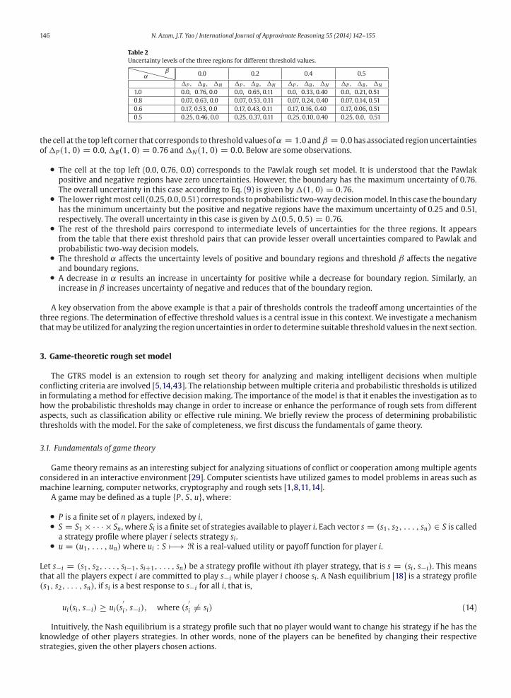
Table 2 shows the uncertainties of the three regions corresponding to different threshold pairs. Each cell in the table

represents three values of the form�P(α, β), �B(α, β), �N(α, β) corresponding to a particular threshold pair. For instance,


Table 2

Uncertainty levels of the three regions for different threshold values.

��αβ 0.0 0.2 0.4 0.5

�P , �B, �N �P , �B, �N �P , �B, �N �P , �B, �N

1.0 0.0, 0.76, 0.0 0.0, 0.65, 0.11 0.0, 0.33, 0.40 0.0, 0.21, 0.51

0.8 0.07, 0.63, 0.0 0.07, 0.53, 0.11 0.07, 0.24, 0.40 0.07, 0.14, 0.51

0.6 0.17, 0.53, 0.0 0.17, 0.43, 0.11 0.17, 0.16, 0.40 0.17, 0.06, 0.51

0.5 0.25, 0.46, 0.0 0.25, 0.37, 0.11 0.25, 0.10, 0.40 0.25, 0.0, 0.51

the cell at the top left corner that corresponds to threshold values ofα = 1.0 andβ = 0.0has associated regionuncertainties

of �P(1, 0) = 0.0, �B(1, 0) = 0.76 and �N(1, 0) = 0.0. Below are some observations.

• The cell at the top left (0.0, 0.76, 0.0) corresponds to the Pawlak rough set model. It is understood that the Pawlak

positive and negative regions have zero uncertainties. However, the boundary has the maximum uncertainty of 0.76.

The overall uncertainty in this case according to Eq. (9) is given by �(1, 0) = 0.76.• The lower rightmost cell (0.25, 0.0, 0.51) corresponds toprobabilistic two-waydecisionmodel. In this case theboundary

has the minimum uncertainty but the positive and negative regions have the maximum uncertainty of 0.25 and 0.51,

respectively. The overall uncertainty in this case is given by �(0.5, 0.5) = 0.76.• The rest of the threshold pairs correspond to intermediate levels of uncertainties for the three regions. It appears

from the table that there exist threshold pairs that can provide lesser overall uncertainties compared to Pawlak and

probabilistic two-way decision models.• The threshold α affects the uncertainty levels of positive and boundary regions and threshold β affects the negative

and boundary regions.• A decrease in α results an increase in uncertainty for positive while a decrease for boundary region. Similarly, an

increase in β increases uncertainty of negative and reduces that of the boundary region.

A key observation from the above example is that a pair of thresholds controls the tradeoff among uncertainties of the

three regions. The determination of effective threshold values is a central issue in this context. We investigate a mechanism

thatmay be utilized for analyzing the region uncertainties in order to determine suitable threshold values in the next section.

3. Game-theoretic rough set model

The GTRS model is an extension to rough set theory for analyzing and making intelligent decisions when multiple

conflicting criteria are involved [5,14,43]. The relationship between multiple criteria and probabilistic thresholds is utilized

in formulating a method for effective decision making. The importance of the model is that it enables the investigation as to

how the probabilistic thresholds may change in order to increase or enhance the performance of rough sets from different

aspects, such as classification ability or effective rule mining. We briefly review the process of determining probabilistic

thresholds with the model. For the sake of completeness, we first discuss the fundamentals of game theory.

3.1. Fundamentals of game theory

Game theory remains as an interesting subject for analyzing situations of conflict or cooperation among multiple agents

considered in an interactive environment [29]. Computer scientists have utilized games to model problems in areas such as

machine learning, computer networks, cryptography and rough sets [1,8,11,14].

A game may be defined as a tuple {P, S, u}, where:

• P is a finite set of n players, indexed by i,• S = S1 ×· · ·× Sn, where Si is a finite set of strategies available to player i. Each vector s = (s1, s2, . . . , sn) ∈ S is called

a strategy profile where player i selects strategy si.• u = (u1, . . . , un) where ui : S −→ � is a real-valued utility or payoff function for player i.

Let s−i = (s1, s2, . . . , si−1, si+1, . . . , sn) be a strategy profile without ith player strategy, that is s = (si, s−i). This means

that all the players expect i are committed to play s−i while player i choose si. A Nash equilibrium [18] is a strategy profile

(s1, s2, . . . , sn), if si is a best response to s−i for all i, that is,

ui(si, s−i) ≥ ui(s′i, s−i), where (s

′i = si) (14)

Intuitively, the Nash equilibrium is a strategy profile such that no player would want to change his strategy if he has the

knowledge of other players strategies. In other words, none of the players can be benefited by changing their respective

strategies, given the other players chosen actions.


Table 3

The strategies to thresholds mapping for the game with a starting values of (α, β) = (1, 0).

Generality

αβ α↓ β↑ α↓β↑

Accuracy

αβ (1.0, 0.0) (0.7, 0.0) (1.0, 0.3) (0.7, 0.3)

α↓ (0.8, 0.0) (0.5, 0.0) (0.8, 0.3) (0.5, 0.3)

β↑ (1.0, 0.2) (0.7, 0.2) (1.0, 0.5) (0.7, 0.5)

α↓β↑ (0.8, 0.2) (0.5, 0.2) (0.8, 0.5) (0.5, 0.5)

3.2. Calculation of probabilistic thresholds with the GTRS model

The GTRS model provides a game-theoretic setting for calculating probabilistic thresholds within the context of proba-

bilistic rough sets. By realizing multiple criteria as players in a game, the model formulates strategies of players in terms

of changes to probabilistic thresholds. Each player will configure the thresholds in order to maximize his benefits. When

strategies are played together and considered as a strategy profile, the individual changes in thresholds are incorporated

to obtain a threshold pair. This means that each strategy profile of the form (s1, s2, . . . , sn) is associated with an (α, β)threshold pair.

We demonstrate the calculation of probabilistic thresholdswith themodel by considering an example game. Considering

the properties of accuracy and generality of the rough set model, a more accuratemodel tends to be less general. In contrast,

a general model may not be very accurate [5]. The two measure were defined earlier in [42]. For a group containing both

positive and negative regions we may defined these measures as,

Accuracy(α, β) = Correctly classified objects by POS(α,β) and NEG(α,β)

Total classified objects by POS(α,β) and NEG(α,β)

, (15)

Generality(α, β) = Total classified objects by POS(α,β) and NEG(α,β)

Number of objects in U. (16)

Changing the threshold levels in order to increase one measure may decrease the other. For instance, the threshold pair

(α, β) = (1, 0) that generates the positive and negative regions with no errors results in maximum accuracy. However,

this configuration may result in fewer objects being classified in the definite regions, leading to poor generality. On the

other hand, the pair (α, β) = (0.5, 0.5) that classify every object in either positive or negative region leads to maximum

generality at a cost of inferior accuracy. Effective threshold values may fall some where between these two extreme cases.

The configuration of thresholds may be realized as a competitive game among these properties.

Let us consider a game involving these two measures as players. Each player may choose from four possible strategies,

namely,

• s1 = αβ (no changes in α and β),• s2 = α↓ (decrease α),• s3 = β↑ (increase β), and• s4 = α↓β↑ (decrease α and increase β).

The game may be played with a starting threshold values of (α, β) = (1, 0). It is known that there is no uncertainty

or classification error in the Pawlak positive POS(1,0) and negative NEG(1,0) regions [38]. That is, the maximum accuracy

corresponds to a threshold configuration of (α, β) = (1, 0). However, in order to find a suitable tradeoff among the two

measures, we allow the accuracy to offer small changes in threshold values. These small changes will safeguard the interests

or benefits of accuracy to a certain level. On the other hand, the generality may consider relatively higher changes in the two

thresholds to increase its benefits. Therefore, we formulated 20% decrease or increase in threshold values for accuracy and

30% for generality.

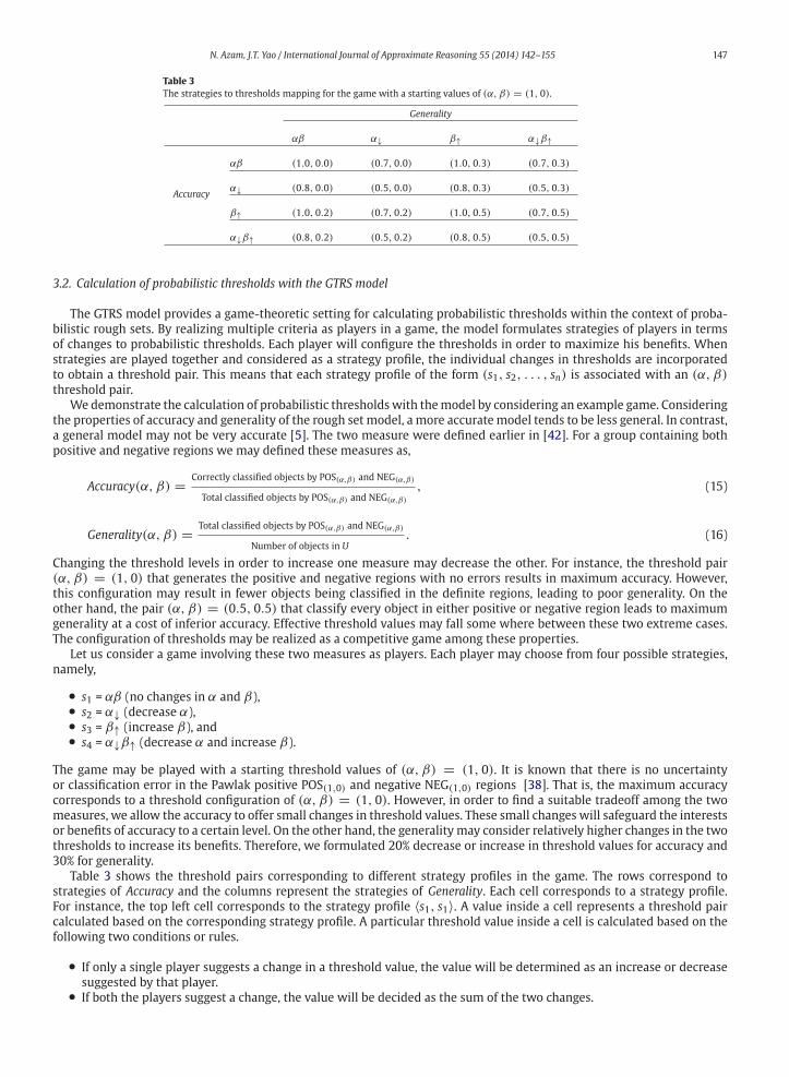
Table 3 shows the threshold pairs corresponding to different strategy profiles in the game. The rows correspond to

strategies of Accuracy and the columns represent the strategies of Generality. Each cell corresponds to a strategy profile.

For instance, the top left cell corresponds to the strategy profile 〈s1, s1〉. A value inside a cell represents a threshold pair

calculated based on the corresponding strategy profile. A particular threshold value inside a cell is calculated based on the

following two conditions or rules.

• If only a single player suggests a change in a threshold value, the value will be determined as an increase or decrease

suggested by that player.• If both the players suggest a change, the value will be decided as the sum of the two changes.


Table 4

Payoff table for the example game.

Generality

αβ α↓ β↑ α↓β↑

Accuracy

αβ (1.0, 0.236) (0.920, 0.413) (0.864, 0.534) (0.852,0.711)

α↓ (0.964, 0.345) (0.864, 0.490) (0.868, 0.643) (0.823, 0.788)

β↑ (0.922, 0.355) (0.893, 0.532) (0.783, 0.746) (0.789, 0.923)

α↓β↑ (0.922, 0.464) (0.851, 0.609) (0.796, 0.855) (0.7711, 1.0)

By applying these rules on initial values of (α, β) = (1, 0), the strategy profile 〈s1, s2〉 = 〈αβ, α↓〉, where Accuracy

plays s1 and Generality plays s2 will correspond to a threshold pair (0.7,0.0). This is represented by the cell that corresponds

to the first row and second column in Table 3.

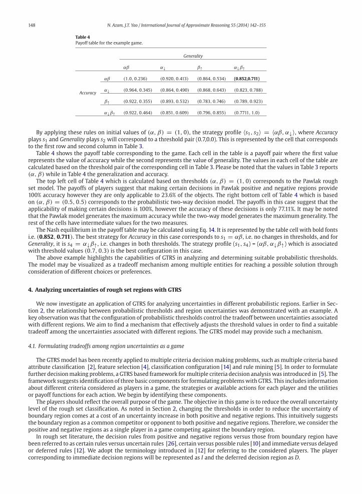
Table 4 shows the payoff table corresponding to the game. Each cell in the table is a payoff pair where the first value

represents the value of accuracy while the second represents the value of generality. The values in each cell of the table are

calculated based on the threshold pair of the corresponding cell in Table 3. Please be noted that the values in Table 3 reports

(α, β) while in Table 4 the generalization and accuracy.

The top left cell of Table 4 which is calculated based on thresholds (α, β) = (1, 0) corresponds to the Pawlak rough

set model. The payoffs of players suggest that making certain decisions in Pawlak positive and negative regions provide

100% accuracy however they are only applicable to 23.6% of the objects. The right bottom cell of Table 4 which is based

on (α, β) = (0.5, 0.5) corresponds to the probabilistic two-way decision model. The payoffs in this case suggest that the

applicability of making certain decisions is 100%, however the accuracy of these decisions is only 77.11%. It may be noted

that the Pawlak model generates the maximum accuracy while the two-waymodel generates the maximum generality. The

rest of the cells have intermediate values for the two measures.

The Nash equilibrium in the payoff table may be calculated using Eq. 14. It is represented by the table cell with bold fonts

i.e. (0.852, 0.711). The best strategy for Accuracy in this case corresponds to s1 = αβ , i.e. no changes in thresholds, and for

Generality, it is s4 = α↓β↑, i.e. changes in both thresholds. The strategy profile (s1, s4) = (αβ, α↓β↑) which is associated

with threshold values (0.7, 0.3) is the best configuration in this case.

The above example highlights the capabilities of GTRS in analyzing and determining suitable probabilistic thresholds.

The model may be visualized as a tradeoff mechanism among multiple entities for reaching a possible solution through

consideration of different choices or preferences.

4. Analyzing uncertainties of rough set regions with GTRS

We now investigate an application of GTRS for analyzing uncertainties in different probabilistic regions. Earlier in Sec-

tion 2, the relationship between probabilistic thresholds and region uncertainties was demonstrated with an example. A

key observation was that the configuration of probabilistic thresholds control the tradeoff between uncertainties associated

with different regions. We aim to find a mechanism that effectively adjusts the threshold values in order to find a suitable

tradeoff among the uncertainties associated with different regions. The GTRS model may provide such a mechanism.

4.1. Formulating tradeoffs among region uncertainties as a game

The GTRSmodel has been recently applied to multiple criteria decisionmaking problems, such as multiple criteria based

attribute classification [2], feature selection [4], classification configuration [14] and rule mining [5]. In order to formulate

further decisionmaking problems, a GTRS based framework formultiple criteria decision analysiswas introduced in [5]. The

framework suggests identification of three basic components for formulating problemswithGTRS. This includes information

about different criteria considered as players in a game, the strategies or available actions for each player and the utilities

or payoff functions for each action. We begin by identifying these components.

The players should reflect the overall purpose of the game. The objective in this game is to reduce the overall uncertainty

level of the rough set classification. As noted in Section 2, changing the thresholds in order to reduce the uncertainty of

boundary region comes at a cost of an uncertainty increase in both positive and negative regions. This intuitively suggests

the boundary region as a common competitor or opponent to both positive and negative regions. Therefore, we consider the

positive and negative regions as a single player in a game competing against the boundary region.

In rough set literature, the decision rules from positive and negative regions versus those from boundary region have

been referred to as certain rules versus uncertain rules [26], certain versus possible rules [10] and immediate versus delayed

or deferred rules [12]. We adopt the terminology introduced in [12] for referring to the considered players. The player

corresponding to immediate decision regions will be represented as I and the deferred decision region as D.


Table 5

Payoff table for the game.

D

s1 = α↓ s2 = β↑ s3 = α↓β↑

I

s1 = α↓ uI(s1,s1),uD(s1,s1) uI(s1,s2),uD(s1,s2) uI(s1,s3),uD(s1,s3)

s2 = β↑ uI(s2,s1),uD(s2,s1) uI(s2,s2),uD(s2,s2) uI(s2,s3),uD(s2,s3)

s3 = α↓β↑ uI(s3,s1),uD(s3,s1) uI(s3,s2),uD(s3,s2) uI(s3,s3),uD(s3,s3)

The players compete in a game with different strategies. The available strategies highlight different options or moves

available to a particular player during the game. Since the players in this game (i.e. the immediate and deferred decision re-

gions) are affected by changes in probabilistic thresholds, we formulate these changes as strategies. Three types of strategies,

namely, s1 = α↓ (decrease of α), s2 = β↑ (increase of β) and s3 = α↓β↑ (decrease of α and increase of β) are considered.

Although the strategies may be formulated in different ways, we considered the case where the configuration starts from

an initial setting of (α, β) = (1, 0) which corresponds to the Pawlak rough set model.

The notion of utility or payoff functions is used to measure the consequences of selecting a particular strategy. The

utilities should reflect possible benefits, performance gains or happiness levels of a particular player. As noted earlier, the

uncertainties of regions are affected by considering different threshold values which are referred to as possible strategies.

Therefore, the levels of uncertainties associated with different regions may be considered as one form of utility or payoff

functions. From a particular player perspective, an uncertainty value reflects a level of loss or disadvantage measured in the

range of 0 to 1. An uncertainty of 1 means an extremely undesirable condition or a minimum possible gain for a player and

an uncertainty of 0 means the most desirable situation. We used the term certainty instead of uncertainty for calculating

the payoff functions to reflect possible gains or benefits of players. The certainty of the three regions are defined as,

CP(α, β) = 1 − �P(α, β),

CN(α, β) = 1 − �N(α, β), and

CB(α, β) = 1 − �B(α, β), (17)

where �P(α, β), �P(α, β) and �P(α, β) are defined in Eq. (9).

For a particular strategy profile (si, sj) that configures the thresholds in order to generate a threshold pair (α, β), theassociated certainty or utility of the players are represented by,

uI(si, sj) = (CP(α, β) + CN(α, β))/2, and

uD(si, sj) = CB(α, β). (18)

where uI and uD represent the payoffs corresponding to immediate and deferred decision regions, respectively. The payoff

is calculated as an average certainty of the two regions, since immediate decision regions include both positive and negative

regions.

4.2. Competition among the regions for analyzing uncertainties

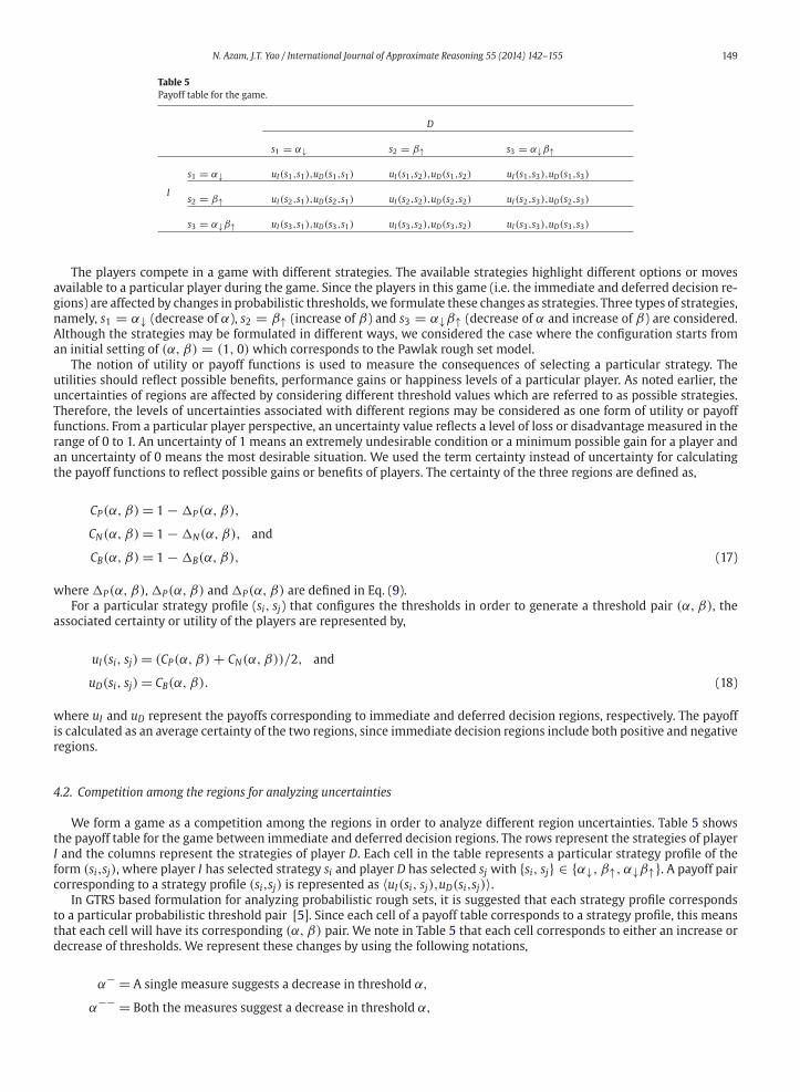
We form a game as a competition among the regions in order to analyze different region uncertainties. Table 5 shows

the payoff table for the game between immediate and deferred decision regions. The rows represent the strategies of player

I and the columns represent the strategies of player D. Each cell in the table represents a particular strategy profile of the

form (si,sj), where player I has selected strategy si and player D has selected sj with {si, sj} ∈ {α↓, β↑, α↓β↑}. A payoff pair

corresponding to a strategy profile (si,sj) is represented as 〈uI(si, sj),uD(si,sj)〉.In GTRS based formulation for analyzing probabilistic rough sets, it is suggested that each strategy profile corresponds

to a particular probabilistic threshold pair [5]. Since each cell of a payoff table corresponds to a strategy profile, this means

that each cell will have its corresponding (α, β) pair. We note in Table 5 that each cell corresponds to either an increase or

decrease of thresholds. We represent these changes by using the following notations,

α− = A single measure suggests a decrease in threshold α,

α−− = Both the measures suggest a decrease in threshold α,


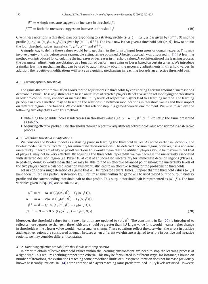
β+ = A single measure suggests an increase in threshold β,

β++ = Both the measures suggest an increase in threshold β. (19)

Given these notations, a threshold pair corresponding to a strategy profile (s1,s1) = (α↓, α↓) is given by (α−−, β) and the

profile (s3,s3) = (α↓β↑, α↓β↑) is given by (α−−, β++). The issue now is that given a threshold pair (α, β), how to obtain

the four threshold values, namely, α−, β+, α−− and β++.

A simple way to define these values would be to get them in the form of input from users or domain experts. This may

involve plenty of trails before some reasonable estimates are obtained. A better approach was discussed in [14]. A learning

methodwas introduced for calculating the increasesordecreases in thresholdvalues.At each iterationof the learningprocess,

the parameter adjustments are obtained as a function of performance gains or losses based on certain criteria. We introduce

a similar learning mechanism that can be used to automatically obtain the necessary adjustments in threshold values. In

addition, the repetitive modifications will serve as a guiding mechanism in reaching towards an effective threshold pair.

4.3. Learning optimal thresholds

The game-theoretic formulation allows for the adjustments in thresholds by considering a certain amount of increase or a

decrease in value. These adjustments are based on utilities of targeted players. Repetitive actions ofmodifying the thresholds

in order to continuously enhance or increase the utility levels of respective players lead to a learning method. The learning

principle in such a method may be based on the relationship between modifications in threshold values and their impact

on different region uncertainties. We consider this relationship in a game-theoretic environment. We wish to achieve the

following two objectives with this method.

• Obtaining the possible increases/decreases in threshold values (i.e. α−, α−−, β+,β++ ) to setup the game presented

as Table 5.• Acquiringeffectiveprobabilistic thresholds throughrepetitiveadjustmentsof thresholdvaluesconsidered inan iterative

process.

4.3.1. Repetitive threshold modifications

We consider the Pawlak model as a starting point in learning the threshold values. As noted earlier in Section 2, the

Pawlak model has zero uncertainty for immediate decision regions. The deferred decision region, however, has a non-zero

uncertainty. In terms of utility or payoff functions this would mean that the utility of player I would be maximum but that

of player D may not be very effective. By adjusting the thresholds repeatedly, we can decrease the uncertainty associated

with deferred decision region (i.e. Player D) at cost of an increased uncertainty for immediate decision regions (Player I).

Repeatedly doing so would mean that we may be able to find an effective balanced point among the uncertainty levels of

the two players. Such a balanced situation will eventually lead to an effective setting for the probabilistic thresholds.

Let us consider a single iteration of a game that will be repeated several times. Suppose that the threshold values (α, β)have been utilized in a particular iteration. Equilibrium analysis within the gamewill be used to find out the output strategy

profile and the corresponding threshold pair to that profile. This output threshold pair is represented as (α′, β

′). The four

variables given in Eq. (19) are calculated as,

α− = α − (α × (CB(α′, β

′) − CB(α, β))),

α−− = α − c(α × (CB(α′, β

′) − CB(α, β))),

β+ = β − (β × (CB(α′, β

′) − CB(α, β))),

β++ = β − c(β × (CB(α′, β

′) − CB(α, β))). (20)

Moreover, the threshold values for the next iteration are updated to (α′, β

′). The constant c in Eq. (20) is introduced to

reflect amore aggressive change in thresholds and should be greater than 1. A larger value for cwouldmean a higher change

in thresholds while a lower value wouldmean a smaller change. These equations reflect the case when the errors in positive

and negative regions are considered as equal. In cases when different weights are assigned to errors in positive and negative

regions, we may consider different constants.

4.3.2. Obtaining effective probabilistic thresholds with stop criteria

In order to obtain effective threshold values within the learning environment, we need to stop the learning process at

a right time. This requires defining proper stop criteria. This may be formulated in different ways, for instance, a bound on

number of iterations, the evaluations reaching some predefined limits or subsequent iteration does not increase previously

knownbest configurations. In [14] a stop criterion of players reaching some predetermined utility levelswas used. However,


this requires the users to provide the stop utility levels according to their beliefs. We utilize a different approach in defining

the stop criteria.

The Pawlak model is considered as a starting point in the learning method. The modifications of thresholds from this

initial setting result in an increase of size for positive region at a cost of associated increase in its uncertainty level. When

the size of probabilistic positive region exceeds the size of actual positive region, wemay suspect that subsequent additions

may cause more misclassifications which may lead to an increase uncertainly level. Thus we set the stop condition as,

P(POS(α,β)(C)) > P(C) = |POS(α,β)(C)||U| >

|C||U| . (21)

Furthermore, when objects are continuously moved from the deferred decision region to immediate decision regions, a

situation may be reached when the boundary becomes empty. This may be realized as a probabilistic two-way decision

model. The modification of thresholds beyond this point may not be very useful. For example, consider (α, β) = (0.5, 0.5),If α is decreased to 0.4, the object x in an equivalence [x] with P(C|[x]) = 0.45 will belong to both positive and negative

regions. This is an undesirable situation fromdecisionmaking perspective. Therefore, in addition to the stop criterion defined

in Eq. (21), we also utilize the stop criterion given by,

P(BND(α,β)(C)) = 0. (22)

Finally, we also want to achieve a superior certainty level for immediate decision regions as compared to the deferred

decision region. From application perspective, a rough setmodel may not be effective if there is greater uncertainty involved

in making immediate or certain decisions against deferred decisions. This leads to a third stop criterion for the learning

algorithm which is defined as,

CP + CN

2< CB = uI < uD. (23)

In summary, we want the learning to stop if any one of the conditions in Eqs. (21)–(23) evaluates to true.

4.3.3. Threshold learning algorithm

Algorithm 1. GTRS based threshold learning algorithm

Input: A data set in the form of an information table.

Initial values of α−, α−−, β+ and β++ for starting the learning process

Output: A threshold pair (α, β).1: Initialize α = 1, β = 0.

2: do

3: For different actions considered in Table 5, calculate the utilities for players D and I according to Eq. (18).

4: Populate the payoff table with calculated values.

5: Perform equilibrium analysis within the payoff tables.

6: Determine the selected actions and the corresponding (α′, β

′) pair.

7: Calculate α−, α−−, β+ and β++ based on threshold pairs (α, β) and (α′, β

′) according to Eq. (20).

8: (α, β) = (α′, β

′)

9: While P(POS(α,β)(C)) ≤ P(C) and P(BND(α,β)(C) = 0 and uI ≥ uD

The above learning procedure can be explained in an algorithmic form. Algorithm 1 is used for this purpose. Given a

particular data set, the algorithm will return an (α, β) pair for classifying objects in the three regions. Line 1 defines the

initial setting or conditions for starting the learning. Line 2 represents a loop. Lines 3–6 represent the use of game-theoretic

analysis in determining a suitable threshold pair. The selected threshold pair is used in lines 7–8 for updating the required

values. Finally, the three stop conditions listed in Eqs. (21)–(23) are given on line 9.

5. Experimental results

Weconducted experiments on20Newsgroup [17] text documents collection. This collection is considered as a benchmark

data set for experiments in text categorization [30,23]. The documents in collection are divided into 20 categories where

each category contains 1000 documents. The categories are named according to their contents. Some of the categories are

very similar in their contents. Table 6 shows a partitioning of the data set into six groups based on the subject of categories.

We used the categories of the first group that discusses the computer related topics. These five categories are shown in bold

in Table 6. Since these categories have equal number of examples, each of them has a prior probability of 1/5 = 0.2.


In selected documents we removed those words that were alphanumeric, had a length of 2 or lesser characters, or were

stopwords (Stopwords, 2010). Porter’s stemming algorithm (Porter, 1980) was also applied to further reduce the vocabulary.

The total number of unique words after preprocessing were 16,266. Since each word is treated as a single feature in text

applications, this leads to a very high dimensional feature space. Feature selection methods are usually adopted to reduce

the feature space by selecting features that have relatively higher level of importance [3].

Itwas argued by [9] that if features are selected efficiently,most of the information is containedwithin the initial features.

This argument got further strength from experimental results reported in [6,24]. It was suggested that reduction of features

set from thousands to hundreds only result in less than 5% decrease of accuracy. Based on these observations, we selected

one hundred features based on chi square feature selection method reported in [33].

We need to represent the textual documents in numeric form for efficient processing on computer machines. The docu-

ment representation scheme of term frequency inverse of document frequency was adopted for this task. Interested reader

may find the details of this representation scheme in [28].

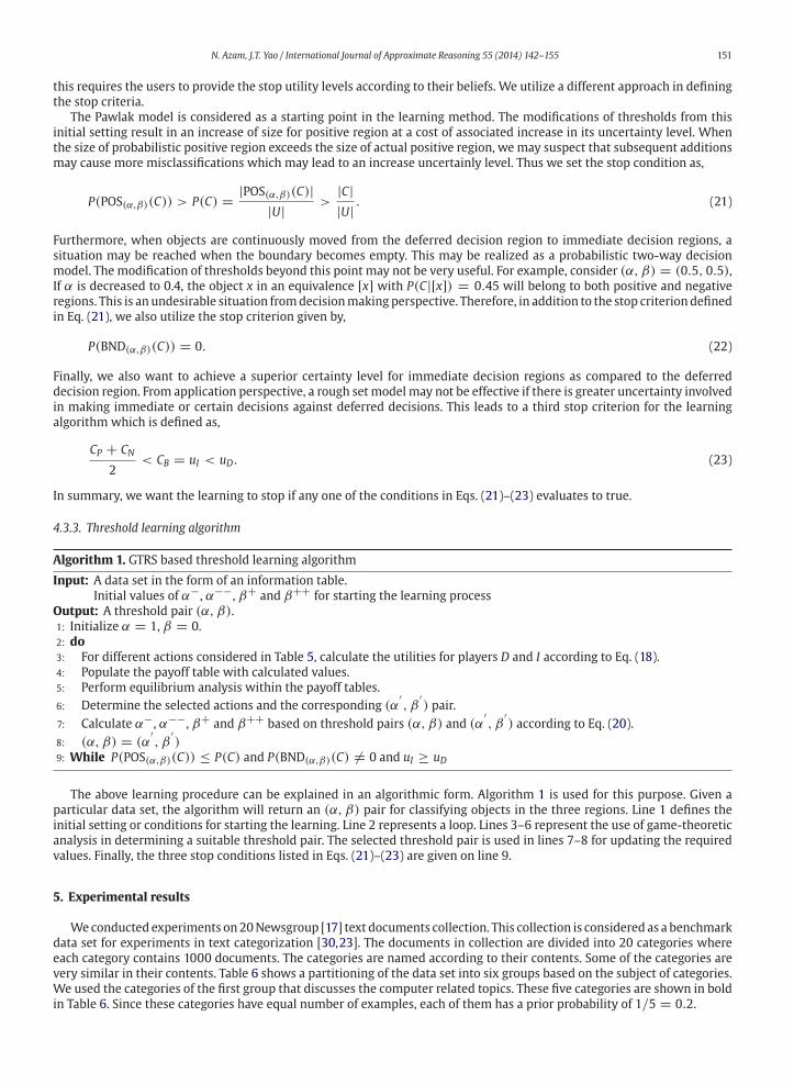
An important issue in thresholds learning algorithm (presented as Algorithm 1) was to setup a proper value for constant

c used in Eq. (20). We tested different values of c and observed the number of iteration for reaching one of the stop criteria.

The number of iterationswere recorded for each category. Table 7 summarizes the results. It shows themaximum,minimum

and average number of iterations for the five categories to the stop conditions. It may be noted that for higher values of c, the

stop conditions are reached in lesser number of iterations. This suggests that higher values of cmaybe useful for reducing the

number of computations. However, according to Eq. (20), higher values of cwould result in drastic changes for the threshold

values. In order to fine tune the thresholds based on the data, one would like to consider relatively lower changes. Moreover,

the small adjustments in thresholds may be useful in increasing the level of accuracy for approximating the regions. We

took into consideration both the number of iterations and fine tunning of thresholds in selecting the constant c. A value of

c = 8 was finally selected for the experiments.

To run the threshold learning algorithm, we need to provide initial values for the variables defined in Eq. (20). We set

the variable values as α− = 0.9, α−− = 0.8, β+ = 0.1 and β++ = 0.2. This means that for the initial game, the

strategy profile (s1,s1) = (α↓, α↓) is given by (α−−, β) = (0.8, 0.0) and the profile (s3,s3) = (α↓β↓, α↓β↓) is given

by (α−−, β++) = (0.8, 0.2). The rest of the threshold pairs corresponding to different strategy profiles can be similarly

obtained as discussed in Section 4. Subsequent games will be generated based on this initial game until one of the stop

criteria is reached.

Table 6

A partition of 20 Newsgroup categories based on their contents.

comp.graphics rec.autos sci.crypt

comp.os.ms-windows.misc rec.motorcycles sci.electronics

comp.sys.ibm.pc.hardware rec.sport.baseball sci.med

comp.sys.mac.hardware rec.sport.hockey sci.space

comp.windows.x

talk.politics.misc talk.religion.misc misc.forsale

talk.politics.guns alt.atheism

talk.politics.mideast soc.religion.christian

Table 7

Constant c and number of iterations.

c

2 3 4 5 6 7 8 9 10

Maximum iterations for a category 171 110 73 56 43 38 33 29 22

Average iterations for categories 124 66 49 38 16 14 11 9 7

Minimum iterations for a category 46 12 16 7 5 4 3 3 2

Table 8

Experimental results for category comp.graphics.

Region size as % of universe Thresholds Certainty

POS BND NEG α β uI uD6.7 57.0 36.3 1.000000 0.000000 1.000000 0.556083

7.0 49.1 43.8 0.800000 0.100000 0.987763 0.593759

7.7 47.5 44.8 0.679437 0.115070 0.978758 0.612012

8.3 46.9 44.8 0.629830 0.123472 0.973806 0.621006

8.6 46.6 44.8 0.584510 0.123472 0.971590 0.624855

8.6 46.6 44.8 0.575511 0.125373 0.971590 0.624855

8.6 46.6 44.8 0.566513 0.127274 0.971590 0.624855

9.1 46.1 44.8 0.548515 0.127274 0.966872 0.632047

9.1 46.1 44.8 0.532737 0.130935 0.966872 0.632047

9.1 46.1 44.8 0.516958 0.134596 0.966872 0.632047

9.1 46.1 44.8 0.501180 0.138257 0.966872 0.632047

11.7 43.5 44.8 0.469623 0.138257 0.946492 0.663352

14.5 36.2 49.3 0.352011 0.155570 0.906372 0.723946

20.2 6.0 73.8 0.266691 0.230982 0.756883 0.952477


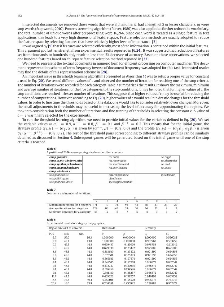
Table 9

Experimental results for category comp.os.ms-windows.misc.



7.9 49.4 42.7 0.800000 0.100000 0.982171 0.603573

13.5 39.0 47.5 0.549938 0.115629 0.924392 0.710590

21.0 4.4 74.6 0.314525 0.214624 0.787120 0.964490

Table 10

Experimental results for category comp.sys.ibm.pc.hardware.



5.7 45.1 49.2 0.800000 0.100000 0.968491 0.601243

9.7 39.3 51.0 0.567078 0.129115 0.933306 0.665694

12.6 34.4 53.0 0.420884 0.195688 0.904675 0.714012

37.2 5.7 57.1 0.258192 0.233509 0.747597 0.953046

Table 11

Experimental results for category comp.sys.mac.hardware.



11.2 39.3 49.5 0.800000 0.100000 0.975973 0.702510

13.4 33.6 53.0 0.483974 0.179006 0.941004 0.757010

14.7 5.2 80.1 0.272959 0.218030 0.804839 0.960176

Table 8 shows the learning results for the category comp.graphics with the GTRS based algorithm. Each row of the table

represents a single iteration of the learning algorithm. From the first row we may note that the initial threshold settings

corresponds to Pawlak model. We have the maximum utility level for player I but not very effective utility for player D.

Different levels of decreases for thresholdα and increases forβ are noted as the learning process continues. These thresholds

adjustments are calculated with game-theoretic analysis discussed earlier. The three regions change in their size based on

calculated threshold values. As the method repeats, the positive and negative regions are growing while boundary region

keeps on shrinking. The algorithm stopswhen the positive region exceeds its prior probability. At this point, the positive and

negative regions has increased in size from 6.7% to 20.2% and from 36.3% to 73.8%, respectively while the boundary region

decreased from 57% to 6%. In the final iteration we note that the certainty level of player D has increased by 40%, (i.e. from

0.55 to 0.95) at a cost of lesser certainty decrease of 25% for player I (i.e. from 1.0 to 0.75).

Table 9 shows the learning results for category comp.os.ms-windows.misc. The algorithm reaches the stop criteria in lesser

number of iterations in this case. From the final configuration of thresholds we note again that the certainty of player D

increase by 40% at a cost of 22% decrease for I. The positive and negative regions increased in their respective sizes from 6.9%

to 21.0% and 38.4% to 74.6%, respectively. The immediate decision making region has been extended from 45.3% to 95.6%.

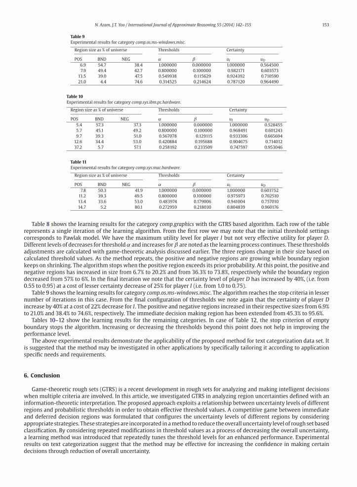
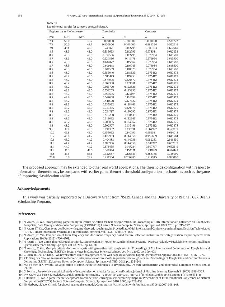
Tables 10–12 show the learning results for the remaining categories. In case of Table 12, the stop criterion of empty

boundary stops the algorithm. Increasing or decreasing the thresholds beyond this point does not help in improving the

performance level.

The above experimental results demonstrate the applicability of the proposed method for text categorization data set. It

is suggested that the method may be investigated in other applications by specifically tailoring it according to application

specific needs and requirements.

6. Conclusion

Game-theoretic rough sets (GTRS) is a recent development in rough sets for analyzing and making intelligent decisions

when multiple criteria are involved. In this article, we investigated GTRS in analyzing region uncertainties defined with an

information-theoretic interpretation. The proposed approach exploits a relationship between uncertainty levels of different

regions and probabilistic thresholds in order to obtain effective threshold values. A competitive game between immediate

and deferred decision regions was formulated that configures the uncertainty levels of different regions by considering

appropriate strategies. These strategies are incorporated inamethod to reduce theoverall uncertainty level of roughsetbased

classification. By considering repeated modifications in threshold values as a process of decreasing the overall uncertainty,

a learning method was introduced that repeatedly tunes the threshold levels for an enhanced performance. Experimental

results on text categorization suggest that the method may be effective for increasing the confidence in making certain

decisions through reduction of overall uncertainty.


Table 12

Experimental results for category comp.windows.x.



7.3 50.0 42.7 0.800000 0.100000 0.989364 0.592216

7.9 49.1 43.0 0.748821 0.112795 0.983133 0.602760

8.5 48.5 43.0 0.685653 0.112795 0.978581 0.612433

8.7 48.3 43.0 0.632596 0.112795 0.976954 0.615500

8.7 48.3 43.0 0.624836 0.114178 0.976954 0.615500

8.7 48.3 43.0 0.617077 0.115562 0.976954 0.615500

8.7 48.3 43.0 0.609318 0.116945 0.976954 0.615500

8.7 48.3 43.0 0.601559 0.118329 0.976954 0.615500

8.8 48.2 43.0 0.586040 0.118329 0.975412 0.617875

8.8 48.2 43.0 0.580473 0.119453 0.975412 0.617875

8.8 48.2 43.0 0.574905 0.120577 0.975412 0.617875

8.8 48.2 43.0 0.569338 0.121701 0.975412 0.617875

8.8 48.2 43.0 0.563770 0.122826 0.975412 0.617875

8.8 48.2 43.0 0.558203 0.123950 0.975412 0.617875

8.8 48.2 43.0 0.552635 0.125074 0.975412 0.617875

8.8 48.2 43.0 0.547068 0.126198 0.975412 0.617875

8.8 48.2 43.0 0.541500 0.127322 0.975412 0.617875

8.8 48.2 43.0 0.535932 0.128446 0.975412 0.617875

8.8 48.2 43.0 0.530365 0.129570 0.975412 0.617875

8.8 48.2 43.0 0.524797 0.130695 0.975412 0.617875

8.8 48.2 43.0 0.519230 0.131819 0.975412 0.617875

8.8 48.2 43.0 0.513662 0.132943 0.975412 0.617875

8.8 48.2 43.0 0.508095 0.134067 0.975412 0.617875

8.8 48.2 43.0 0.502527 0.135191 0.975412 0.617875

9.6 47.4 43.0 0.491392 0.135191 0.967927 0.627119

10.2 46.8 43.0 0.455052 0.140190 0.962581 0.634013

10.2 45.6 44.2 0.429953 0.144056 0.956609 0.641504

10.6 45.2 44.2 0.404188 0.144056 0.952263 0.646839

11.1 44.7 44.2 0.386936 0.144056 0.947717 0.652319

11.1 44.7 44.2 0.378455 0.147214 0.947717 0.652319

11.1 41.3 47.6 0.369974 0.150371 0.931889 0.674149

13.8 33.1 53.1 0.337667 0.176633 0.885385 0.738090

20.8 0.0 79.2 0.251304 0.266985 0.717945 1.000000

The proposed approach may be extended to other real world applications. The thresholds configuration with respect to

information-theoreticmay be comparedwith earlier game-theoretic threshold configurationmechanisms, such as the game

of improving classification ability.

Acknowledgements

This work was partially supported by a Discovery Grant from NSERC Canada and the University of Regina FGSR Dean’s

Scholarship Program.

References

[1] N. Azam, J.T. Yao, Incorporating game theory in feature selection for text categorization, in: Proceeding of 13th International Conference on Rough Sets,Fuzzy Sets, Data Mining and Granular Computing (RSFDGrC’11), Lecture Notes in Computer Science, Springer, vol. 6743, 2011, pp. 215–222.

[2] N. Azam, J.T. Yao, Classifying attributes with game-theoretic rough sets, in: Proceedings of 4th International Conference on Intelligent Decision Technologies(IDT’12), Smart Innovation, Systems and Technologies, Springer, vol. 15, 2012, pp. 175–184.

[3] N. Azam, J.T. Yao, Comparison of term frequency and document frequency based feature selection metrics in text categorization, Expert Systems with

Applications 39 (5) (2012) 4760–4768.[4] N. Azam, J.T. Yao, Game-theoretic rough sets for feature selection, in: RoughSets and Intelligent Systems–Professor ZdzislawPawlak inMemoriam, Intelligent

Systems Reference Library, Springer, vol. 44, 2012, pp. 61–78.[5] N. Azam, J.T. Yao, Multiple criteria decision analysis with game-theoretic rough sets, in: Proceedings of 7th International Conference on Rough Sets and

Knowledge Techonology (RSKT’12), Lecture Notes in Computer Science, Springer, vol. 7414, 2012, pp. 399–408.[6] C. Chen, H. Lee, Y. Chang, Two novel feature selection approaches for web page classification, Expert Systems with Applications 36 (1) (2012) 260–272.

[7] X.F. Deng, Y.Y. Yao, An information-theoretic interpretation of thresholds in probabilistic rough sets, in: Proceedings of Rough Sets and Current Trends in

Computing (RSCTC’12), Lecture Notes in Computer Science, Springer, vol. 7413, 2012, pp. 232–241.[8] M.J. Fischer, R.N. Wright, An application of game theoretic techniques to cryptography, Discrete Mathematics and Theoretical Computer Science (1993)

99–118.[9] G. Forman, An extensive empirical study of feature selection metrics for text classification, Journal of Machine Learning Research 3 (2003) 1289–1305.

[10] J.W. Grzymala-Busse, Knowledge acquisition under uncertainty – a rough set approach, Journal of Intelligent and Robotic Systems 1 (1) (1988) 3–16.[11] J. Herbert, J.T. Yao, A game-theoretic approach to competitive learning in self-organizing maps, in: Proceedings of 1st International Conference on Natural

Computation (ICNC’05), Lecture Notes in Computer Science, Springer, vol. 3610, 2005, pp. 129–138.

[12] J.P. Herbert, J.T. Yao, Criteria for choosing a rough set model, Computers & Mathematics with Applications 57 (6) (2009) 908–918.


[13] J.P. Herbert, J.T. Yao, Analysis of data-driven parameters in game-theoretic rough sets, in: Proceedings of 6th International Conference Rough Sets andKnowledge Technology (RSKT’11), Lecture Notes in Computer Science, Springer, vol. 6954, 2011, pp. 447–456.

[14] J.P. Herbert, J.T. Yao, Game-theoretic rough sets, Fundamenta Informaticae 108 (3–4) (2011) 267–286.[15] X.Y. Jia, W.W. Li, L. Shang, J.J. Chen, An optimization viewpoint of decision-theoretic rough set model, in: Proceedings of 6th International Conference on

Rough Sets and Knowledge Technology (RSKT’11), Lecture Notes in Computer Science, Springer, vol. 6954, 2011, pp. 457–465.

[16] X.Y. Jia, Z.M. Tang, W.L. Liao, L. Shang, On an optimization representation of decision-theoretic rough set model, International Journal of ApproximateReasoning (2013). http://dx.doi.org/10.1016/j.ijar.2013.02.010.

[17] K. Lang, Newsweeder: learning to filter netnews, in: Proceedings of the 12th International Conference on Machine Learning (ICML’95), 1995, pp. 331–339.[18] K. Leyton-Brown, Y. Shoham, Essentials of Game Theory: A Concise Multidisciplinary Introduction, Morgan & Claypool Publishers, 2008.

[19] H.X. Li, X.Z. Zhou, Risk decision making based on decision-theoretic rough set: a three-way view decision model, International Journal of ComputationalIntelligence Systems 4 (1) (2011) 1–11.

[20] T.J. Li, X.P. Yang, An axiomatic characterization of probabilistic rough sets, International Journal of Approximate Reasoning (2013).

http://dx.doi.org/10.1016/j.ijar.2013.02.012.[21] D. Liu, T.R. Li, D. Liang, Incorporating logistic regression to decision-theoretic rough sets for classifications, International Journal of Approximate Reasoning

(2013). http://dx.doi.org/10.1016/j.ijar.2013.02.013.[22] D. Liu, T.R. Li, D. Ruan, Probabilistic model criteria with decision-theoretic rough sets, Information Science 181 (17) (2011) 3709–3722.

[23] Y. Miao, M. Kamel, Pairwise optimized rocchio algorithm for text categorization, Pattern Recognition Letters 32 (2) (2011) 375–382.[24] H. Ogura, H. Amano, M. Kondo, Feature selection with a measure of deviations from poisson in text categorization, Expert Systems with Applications 36 (3)

(2009) 6826–6832.

[25] Z. Pawlak, Rough sets, International Journal of Computer and Information Sciences 11 (1982) 241–256.[26] Z. Pawlak, Rough sets, decision algorithms and Bayes’ theorem, European Journal of Operational Research 136 (1) (2002) 181–189.

[27] Y. Qian, H. Zhang, Y. Sang, J. Liang, Multigranulation decision-theoretic rough sets, International Journal of Approximate Reasoning (2013).http://dx.doi.org/10.1016/j.ijar.2013.03.004.

[28] F. Sebastiani, Machine learning in automated text categorization, ACM Computing Surveys 34 (1) (2002) 1–47.[29] J. Von Neumann, O. Morgenstern, H. Kuhn, A. Rubinstein, Theory of Games and Economic Behavior (Commemorative Edition), Princeton University Press,

2007.

[30] J. Yang, Y. Liu, X. Zhu, Z. Liu, X. Zhang, A new feature selection based on comprehensive measurement both in inter-category and intra-category for textcategorization, Information Processing Management 48 (4) (2012) 741–754.

[31] X.P. Yang, J.T. Yao, A multi-agent decision-theoretic rough set model, in: Proceedings of 5th International Conference Rough Set and Knowledge Technology(RSKT’10), Lecture Notes in Computer Science, Springer, vol. 6401, 2010, pp. 711–718.

[32] X.P. Yang, J.T. Yao, Modelling multi-agent three-way decisions with decision-theoretic rough sets, Fundamenta Informaticae 115 (2–3) (2012) 157–171.[33] Y. Yang, J.O. Pedersen, A comparative study on feature selection in text categorization, in: Proceedings of the 14th International Conference on Machine

Learning (ICML’97), 1997, pp. 412–420.[34] J.T. Yao, A. Vasilakos, W. Pedrycz, Granular computing: perspectives and challenges, IEEE Transactions on Cybernetics (2013).

http://dx.doi.org/10.1109/TSMCC.2012.2236648.

[35] J.T. Yao, Y.Y. Yao, W. Ziarko, Probabilistic rough sets: approximations, decision-makings, and applications, International Journal of Approximate Reasoning49 (2) (2008) 253–254.

[36] Y.Y. Yao, Decision-theoretic rough set models, in: Proceedings of Second International Conference on Rough Sets and Knowledge Technology (RSKT’07),Lecture Notes in Computer Science, Springer, vol. 4481, 2007, pp. 1–12.

[37] Y.Y. Yao, Probabilistic rough set approximations, International Journal of Approximate Reasoning 49 (2) (2008) 255–271.[38] Y.Y. Yao, Three-way decisions with probabilistic rough sets, Information Science 180 (3) (2010) 341–353.

[39] Y.Y. Yao, The superiority of three-way decisions in probabilistic rough set models, Information Sciences 181 (6) (2011) 1080–1096.

[40] Y.Y. Yao, Two semantic issues in a probabilistic rough set model, Fundamenta Informaticae 108 (3–4) (2011) 249–265.[41] Y.Y. Yao, An outline of a theory of three-way decisions, in: Proceedings of Rough Sets and Current Trends in Computing (RSCTC’12), LectureNotes in Computer

Science, Springer, vol. 7413, 2012, pp. 1–17.[42] Y.Y. Yao, Y. Zhao, Attribute reduction in decision-theoretic rough set models, Information Sciences 178 (17) (2008) 3356–3373.

[43] Y. Zhang, J.T. Yao, Rule measures tradeoff using game-theoretic rough sets, in: Proceedings of International Conference on Brian Informatics (BI’12), LectureNotes in Computer Science, Springer, vol. 7670, 2012, pp. 348–359.

doi:10.1016/j.ijar.2013.02.010

doi:10.1016/j.ijar.2013.02.012

doi:10.1016/j.ijar.2013.02.013

doi:10.1016/j.ijar.2013.03.004

doi:10.1109/TSMCC.2012.2236648

Documents

Analyzing uncertainties of probabilistic rough set regions with game-theoretic rough sets