Embed Size (px)
Citation preview
HAL Id: tel-03420626https://tel.archives-ouvertes.fr/tel-03420626
Submitted on 9 Nov 2021
HAL is a multi-disciplinary open accessarchive for the deposit and dissemination of sci-entific research documents, whether they are pub-lished or not. The documents may come fromteaching and research institutions in France orabroad, or from public or private research centers.
L’archive ouverte pluridisciplinaire HAL, estdestinée au dépôt et à la diffusion de documentsscientifiques de niveau recherche, publiés ou non,émanant des établissements d’enseignement et derecherche français ou étrangers, des laboratoirespublics ou privés.
Anchored solutions in robust combinatorial optimizationAdèle Pass-Lanneau
To cite this version:Adèle Pass-Lanneau. Anchored solutions in robust combinatorial optimization. Operations Research[cs.RO]. Sorbonne Université, 2021. English. �NNT : 2021SORUS177�. �tel-03420626�
Ecole Doctorale Informatique, Telecommunications et Electronique, Paris
Sorbonne Universite, Laboratoire LIP6, equipe Recherche Operationnelle
EDF R&D, departement OSIRIS
Anchored solutionsin robust combinatorial optimization
Adele Pass-Lanneau
These de doctorat en informatiquepresentee et soutenue publiquement le 16 mars 2021
Jury
Rapporteurs
Dominique De Werra Professeur honoraire, EPFL, Suisse
Gerhard J. Woeginger Professeur, RWTH Aachen, Allemagne
Examinateurs
Bruno Escoffier Professeur, Sorbonne Universite, LIP6, France
Frederic Meunier Professeur, Ecole des Ponts, CERMICS, France
Michael Poss Directeur de recherche, CNRS, LIRMM, France
Encadrants
Pascale Bendotti Ingenieur-Chercheur HDR, EDF R&D, France
Philippe Chretienne Professeur emerite, Sorbonne Universite, LIP6, France
Pierre Fouilhoux Professeur, Universite Sorbonne Paris Nord, LIPN, France

Extended abstract
An instance of an optimization problem is often subject to uncertainty and likely tochange over time. If the instance changes, an optimal solution to the instance alsochanges. However, changing a solution could be difficult in practice. The decisionmaker may be change-averse and prefer solutions that are, in some sense, stable.In this thesis we investigate a stability criterion based on anchored decisions, thatare unchanged decisions with respect to a baseline solution. In reoptimization, thegoal is to find a new solution with a maximum number of decisions maintainedfrom the previously computed baseline solution. In robust optimization, it is tofind in advance a baseline solution along with a subset of anchored decisions.When the solution must be modified to adapt to instance disruptions within agiven uncertainty set, anchored decisions are guaranteed not to change.
In Part I, the generic concepts of the thesis are proposed and compared withthe literature. In Chapter 1 we first review the state of the art in robust opti-mization and solution stability. In Chapter 2, the concepts are presented. Theanchoring level is defined as the number of identical decisions between two so-lutions of a discrete optimization problem. Anchor-reoptimization problems aredefined, where the anchoring level is maximized. Anchor-robust problems are thendefined as 2-stage robust problems where the size of the subset of anchored deci-sions is maximized. Anchor-robustness fills the gap between static-robustness andadjustable-robustness, as it allows to find a trade-off between the cost of a baselinesolution and the number of anchored decisions.
Anchor-reoptimization and anchor-robust problems are studied on two classesof problems: combinatorial problems with only binary variables in Part II, andscheduling problems with continuous variables in Part III and Part IV.
In Part II, we consider combinatorial problems written as integer programs inbinary variables, such as matroid bases or matchings. Chapter 3 is devoted toanchor-reoptimization, under the form of k-red problems from the literature. Wefocus on anchor-reoptimization for matroid bases, which can be solved in polyno-mial time, either by a lagrangian-based algorithm or using a polyhedral characteri-zation. In Chapter 4, anchor-robustness for combinatorial problems is investigated.
3
Extended abstract
The complexity of the anchor-robust problem is analyzed for various uncertaintysets, and an MIP reformulation is obtained. The anchor-robust problem is shownto be computationally less demanding than the recoverable robust problem fromthe literature. Finally the so-called price of anchor-robustness is studied, which isthe overhead cost of an anchor-robust solution with respect to a recoverable robustsolution.
In Part III, we consider project scheduling problems, that involve continu-ous decision variables. In Chapter 5, reoptimization is first considered, by themeans of anchored rescheduling problems. The complexity of rescheduling forvarious project scheduling problems is analyzed, showing the boundary betweenpolynomial and hard cases of anchored rescheduling problems. In Chapter 6, theanchor-robust approach is developed for project scheduling under precedence con-straints, leading to the AnchRobPSP problem. Combinatorial properties of theproblem are studied, and dedicated graph models are proposed. We then study thecomplexity of AnchRobPSP. Several cases of AnchRobPSP are shown NP-hard,including budgeted uncertainty. Algorithms are designed for polynomial cases.For budgeted uncertainty an MIP reformulation is obtained, and its numericalperformance is assessed. In Chapter 7, the anchor-robust approach is redesignedto address the Resource-Constrained Project Scheduling Problem (RCPSP), whichis already NP-hard in a deterministic setting. We show the connection with theAdjustable-Robust RCPSP from the literature. Algorithmic tools are proposed,building upon the contributions of Chapter 6. Exact MIP-based approaches anddedicated heuristics are devised, for both the Adjustable-Robust RCPSP and theAnchor-Robust RCPSP in a unified way. The proposed exact and heuristic ap-proaches are thoroughly evaluated on benchmark instances. Finally, a use case ofanchor-robustness in project scheduling is presented, on a maintenance planningproblem arising at EDF.
In Part IV, we further investigate mixed-integer programming techniques forthe AnchRobPSP problem introduced in Part III. The formulation from Chapter 6is investigated, together with new linear formulations valid for a larger variety ofuncertainty sets. In Chapter 8, a dominance property is exhibited, and a newcompact formulation is proposed. We show that it captures the combinatorialstructure of the problem. Indeed it yields a polyhedral characterization of integersolutions of AnchRobPSP in non-trivial cases. Numerical experiments are carriedout to show the efficiency of the approach on instances close to characterizationcases, and on new uncertainty sets. In Chapter 9, we investigate formulationsin the space of anchoring variables only. A complete picture of formulations forAnchRobPSP is given, both in anchoring variables only, and in extended formwith additional schedule variables. A facial study of the anchored set polytopeis then proposed. In cases where a polyhedral characterization was previously
4
Extended abstract
obtained, we give a minimal description of the anchored set polytope. In generalcase, new inequalities are exhibited to strengthen inequalities from the proposedlinear formulations.
Finally conclusions and research perspectives are presented. We point outsome open complexity questions on the anchor-reoptimization and anchor-robustproblems studied in the thesis, and give perspectives on the design of efficient algo-rithms for NP-hard cases. Finally other problems are identified where the conceptof anchored solutions is relevant, and would lead to new anchor-reoptimizationand anchor-robust problems.
5

Extended abstract
6
Contents
Extended abstract 3
I Anchored solutions in robust optimization 11
Preliminaries 13
1 Robust optimization: state of the art 15
1.1 Robustness in discrete optimization . . . . . . . . . . . . . . . . . . 15
1.2 Static robustness . . . . . . . . . . . . . . . . . . . . . . . . . . . . 18
1.3 Two-stage robust optimization . . . . . . . . . . . . . . . . . . . . . 22
1.4 Solution stability in reoptimization and robust optimization . . . . 27
2 Anchored solutions: concepts 33
2.1 Anchoring level . . . . . . . . . . . . . . . . . . . . . . . . . . . . . 33
2.2 Anchor-Reoptimization . . . . . . . . . . . . . . . . . . . . . . . . . 35
2.3 Anchor-Robust optimization . . . . . . . . . . . . . . . . . . . . . . 39
2.4 Main research directions . . . . . . . . . . . . . . . . . . . . . . . . 47
II Anchored solutions to combinatorial problems 49
Preliminaries 51
3 Anchor-Reoptimization for combinatorial problems:a case study on matroid bases 53
3.1 k-red matroid bases . . . . . . . . . . . . . . . . . . . . . . . . . . . 56
3.2 Illustration for the k-red spanning tree . . . . . . . . . . . . . . . . 63
3.3 k-red bipartite matching . . . . . . . . . . . . . . . . . . . . . . . . 65
7
Contents
4 Anchor-Robustness for combinatorial problems 69
4.1 Definitions . . . . . . . . . . . . . . . . . . . . . . . . . . . . . . . . 69
4.2 Complexity for discrete and polyhedral uncertainty sets . . . . . . . 73
4.3 MIP reformulations . . . . . . . . . . . . . . . . . . . . . . . . . . . 77
4.4 The price of anchor-robustness . . . . . . . . . . . . . . . . . . . . . 81
III Anchored solutions in project scheduling 87
Preliminaries 89
5 Anchored Rescheduling problems for project scheduling 91
5.1 Anchored rescheduling under generalized precedence . . . . . . . . . 91
5.2 Polynomiality of ε-AnchRe(GenPrec) . . . . . . . . . . . . . . . . 94
5.3 Anchored rescheduling with a deadline constraint . . . . . . . . . . 96
5.4 Sensitivity analysis with respect to tolerance . . . . . . . . . . . . . 97
5.5 Towards machine rescheduling . . . . . . . . . . . . . . . . . . . . . 99
6 The Anchor-Robust Project Scheduling Problem 103
6.1 The Anchor-Robust Project Scheduling Problem . . . . . . . . . . . 104
6.2 Graph models for AnchRobPSP . . . . . . . . . . . . . . . . . . . . 110
6.3 Complexity of the AnchRobPSP . . . . . . . . . . . . . . . . . . . . 116
6.4 Algorithms for special cases of AnchRobPSP . . . . . . . . . . . . . 121
6.5 Comparison to affine decision rules . . . . . . . . . . . . . . . . . . 127
6.6 Numerical results . . . . . . . . . . . . . . . . . . . . . . . . . . . . 132
7 The Anchor-Robust RCPSP: exact and heuristic approaches 145
7.1 Preliminaries . . . . . . . . . . . . . . . . . . . . . . . . . . . . . . 146
7.2 Anchor-Robust approach for the RCPSP . . . . . . . . . . . . . . . 147
7.3 Graph model and compact MIP reformulations . . . . . . . . . . . . 153
7.4 Computational results: MIP for Adjustable-Robust RCPSP . . . . . 161
7.5 Computational results: Heuristics for Adjustable-Robust RCPSP . . 165
7.6 Computational results: MIP for Anchor-Robust RCPSP . . . . . . 171
7.7 Computational results: Heuristic for Anchor-Robust RCPSP . . . . 175
Industrial use case 179
IV Polyhedral approaches for AnchRobPSP 183
Preliminaries 185
8
Contents
8 Dominance-based linear formulation for AnchRobPSP 1878.1 Preliminaries on uncertainty sets . . . . . . . . . . . . . . . . . . . 1888.2 Linear formulations for AnchRobPSP . . . . . . . . . . . . . . . . . 1908.3 Polyhedral characterization for special cases . . . . . . . . . . . . . 1958.4 Numerical results . . . . . . . . . . . . . . . . . . . . . . . . . . . . 201
9 The combinatorial structure of AnchRobPSP 2119.1 Formulations in anchoring variables . . . . . . . . . . . . . . . . . . 2119.2 Polyhedral study of the polytope of anchored sets . . . . . . . . . . 2219.3 Linear bounds evaluation . . . . . . . . . . . . . . . . . . . . . . . . 226
Conclusion and research perspectives 231
Appendix 235
Bibliography 239
9

Contents
10

Part I
Anchored solutions in robustoptimization
11

Preliminaries on optimization problems
We consider discrete optimization problems under the following form:
(P) min cTx
s.t. x ∈ X
The decision variables are coordinates of decision vector x ∈ RI with I a set of|I| = n decisions. The objective is to minimize a linear cost function cTx, withcost vector c ∈ RI . The feasible set is X ⊆ RI
+. An instance of problem (P) is thus(c,X ). We assume that problem (P) can be written as a mixed-integer program(MIP) under the following form
(MIP) min cTx
s.t. Ax ≤ b
x ≥ 0
x ∈ {0, 1}q × Rn−q
where matrix A is the constraint matrix, and vector b the right-hand side. Decisionvariables xi, i ∈ {1, . . . , q} are binary variables, while decision variables xi, i ∈{q+ 1, . . . , n} are continuous variables. Let S denote the space where the decisionvector lies, that is, S = {0, 1}q × Rn−q. If all decision variables are continuous,i.e., S = RI , (MIP) is a linear program. If all decision variables are binary, i.e.,S = {0, 1}I , (MIP) is an integer program in binary variables. In particular, wesay that (P) is a combinatorial problem if it can be written as (MIP) with binaryvariables only.
Let us introduce three problems: Selection, Min Cost Spanning Treeand PERT Scheduling. These problems will be used in Chapter 1 and Chapter 2to illustrate the proposed concepts. Selection, Min Cost Spanning Treeare combinatorial problems, while PERT Scheduling has continuous decisionvariables. All three are polynomially solvable.
13
Selection. Consider a set of n items. Each item i ∈ {1, . . . , n} is associatedwith cost ci ≥ 0. Let p be an integer, p ≤ n. The Selection problem is to selectp items, so as to minimize the total cost of selected items. With binary decisionvariable xi = 1 if item i is selected, xi = 0 otherwise, the problem writes as
min cTx
s.t.∑n
i=1 xi = p
x ∈ {0, 1}n
Note that an optimal solution to Selection is simply obtained by sorting theitems in increasing order of costs ci, and selecting the first p items.
Min Cost Spanning Tree. Consider a graph G = (V,E). A spanningtree is a subset T ⊆ E of edges such that T is cycle-free and |T | = |V | − 1.Consider a vector of costs associated to edges c ∈ RE
+. The Min Spanning Treeproblem is to find a spanning tree T ⊆ E with minimum total cost. Considerbinary decision variable xe = 1 if edge e is in the tree, xe = 0 otherwise. Theproblem writes as min cTx for x ∈ X , where X ⊆ {0, 1}E is the set of incidencevectors of spanning trees. Classically the set X can be described with a familyof linear inequalities (see, e.g., (Schrijver, 2003)), and this family has exponentialsize. A min-cost spanning tree can be found algorithmically in polynomial timewith Kruskal’s algorithm (see, e.g., (Korte and Vygen, 2012)).
PERT Scheduling. Consider a project with a set J of n jobs. Let s andt two dummy jobs representing the beginning and the end of the project, andJ = J ∪{s, t}. Consider a set of precedence relations, represented by a precedencegraph (J,A). It is assumed that the precedence graph is acyclic, and s (resp. t) isa predecessor (resp. a successor) of all jobs. Each job has a processing time pi ≥ 0.A schedule is a vector of starting times xi ≥ 0, i ∈ J of the jobs. The makespan ofschedule is xt. The Project Scheduling Problem, or PERT SchedulingProblem, is to find a schedule x ∈ RJ
+ such that for every precedence relation(i, j) ∈ A, job j starts after job i completes, and so as to minimize the makespanxt. The problem writes as
min xts.t. xj − xi ≥ pi ∀(i, j) ∈ A
x ≥ 0
x ∈ RJ
It is a linear program, and as such, it is solvable in polynomial time. The optimalvalue of the problem is equal to the longest s−t path in the precedence graph(Pinedo, 2002). This longest path value can be computed in polynomial time bydynamic programming.
14
Chapter 1
Robust optimization: state of theart
In this chapter, we present state-of-the-art concepts in robust optimization andsolution stability in which the contributions of the thesis fit. In Section 1.1 thegeneral principles of robustness are exposed. In Section 1.2 and Section 1.3,static-robust optimization and two-stage robust optimization are presented. InSection 1.4 related work on solution stability is reviewed.
1.1 Robustness in discrete optimization
Let us first present the core principles of robust optimization, and present the ideaof uncertainty sets.
1.1.1 Robust optimization basics
Discrete optimization is commonly used in operations research to represent a real-life problem. It may come from various applicative fields, such as schedulingand planning, workforce assignment, or network design. This real-life problem isrepresented by an instance of a discrete optimization problem.
However in practice data is often not known exactly. Data can be difficultto measure or estimate: hence it is not known with perfect accuracy. Data canalso be dynamic and change over time. Then at some point in time, some data isavailable which will not be accurate anymore in the future. This occurs when datais acquired in advance, before the solution of the optimization problem is usedfor practical implementation. Data inaccuracy raises the question of handlinguncertainty in optimization problems. It is all the more important because theconsidered discrete optimization problems are very sensitive to uncertainty. A
15
Chapter 1. Robust optimization: state of the art
disruption in the constraints or objective function, be it very small, may impairthe optimality or feasibility of a solution. Therefore one cannot solve the originaloptimization problem being oblivious to uncertainty, then hope that the solutionwill behave well if data changes, even “not too much”. Uncertainty must beintegrated from the start into the optimization process, with full awareness.
The two main trends for optimization under uncertainty are stochastic op-timization and robust optimization. The present work lies in the scope of thelatter. In stochastic optimization, distributional information of uncertain data isavailable, and a stochastic criterion (e.g., the expected value) is optimized. Theparadigm of robust optimization is to consider that unknown data may take anyvalue in a so-called uncertainty set. By contrast with stochastic optimization, nofurther information is available on distribution of data in the uncertainty set. Ro-bust optimization is then to find solutions that are immune to any realization inthe uncertainty set, and to optimize a worst-case criterion. Those two ingredientsof robust optimization, i.e., an uncertainty set, and a worst-case criterion, werealready mentioned in early work, such as the book from Kouvelis and Yu (1996),Robust Discrete Optimization and Its Applications :
“We suggest the use of the robustness approach to decision making, which as-sumes inadequate knowledge [...] about the random state of nature and developsa decision that hedges against the worst contingency that may arise.”
1.1.2 Uncertainty sets
Let us formalize the idea of uncertainty set. We want to account for uncertaintyon numerical data of the mixed-integer program (MIP), that is, coefficients in theconstraints or objective function.
The constraint matrix, right-hand side, and cost vector are considered to havenominal values A, b, and c. The instance of (MIP) with nominal values as datacorresponds to the deterministic problem. We then consider that the real datamay deviate from the nominal values, to be equal to A + δA, b + δb, c + δc. Thedeviations δA, δb, δc are a matrix and vectors with the same sizes as A, b, c. Anuncertainty realization is δ = (δA, δb, δc). The uncertainty set ∆ is a set containingall uncertainty realizations δ = (δA, δb, δc) that the decision maker wants to hedgeagainst.
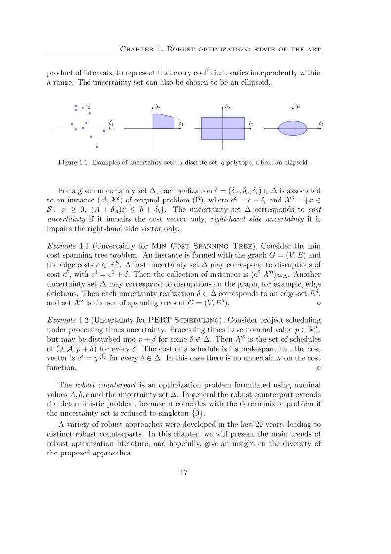
There are a number of options for the geometry of the uncertainty set, asillustrated in Figure 1.1. It can be a discrete set, then every uncertainty realizationis said to be a scenario. The uncertainty set can also be a convex set, usuallycontaining the element where all deviations are zero. For example, it can bechosen to be a polyhedron. A special case of polyhedron is a box, i.e., a cartesian
16
Chapter 1. Robust optimization: state of the art
product of intervals, to represent that every coefficient varies independently withina range. The uncertainty set can also be chosen to be an ellipsoid.
δ1
δ2
•
••
••
••
•• •
δ1
δ2
δ1
δ2
δ1
δ2
Figure 1.1: Examples of uncertainty sets: a discrete set, a polytope, a box, an ellipsoid.
For a given uncertainty set ∆, each realization δ = (δA, δb, δc) ∈ ∆ is associatedto an instance (cδ,X δ) of original problem (P), where cδ = c + δc and X δ = {x ∈S : x ≥ 0, (A + δA)x ≤ b + δb}. The uncertainty set ∆ corresponds to costuncertainty if it impairs the cost vector only, right-hand side uncertainty if itimpairs the right-hand side vector only.
Example 1.1 (Uncertainty for Min Cost Spanning Tree). Consider the mincost spanning tree problem. An instance is formed with the graph G = (V,E) andthe edge costs c ∈ RE
+. A first uncertainty set ∆ may correspond to disruptions ofcost cδ, with cδ = c0 + δ. Then the collection of instances is (cδ,X 0)δ∈∆. Anotheruncertainty set ∆ may correspond to disruptions on the graph, for example, edgedeletions. Then each uncertainty realization δ ∈ ∆ corresponds to an edge-set Eδ,and set X δ is the set of spanning trees of G = (V,Eδ). �
Example 1.2 (Uncertainty for PERT Scheduling). Consider project schedulingunder processing times uncertainty. Processing times have nominal value p ∈ RJ
+,but may be disturbed into p + δ for some δ ∈ ∆. Then X δ is the set of schedulesof (J,A, p + δ) for every δ. The cost of a schedule is its makespan, i.e., the costvector is cδ = χ{t} for every δ ∈ ∆. In this case there is no uncertainty on the costfunction. �
The robust counterpart is an optimization problem formulated using nominalvalues A, b, c and the uncertainty set ∆. In general the robust counterpart extendsthe deterministic problem, because it coincides with the deterministic problem ifthe uncertainty set is reduced to singleton {0}.
A variety of robust approaches were developed in the last 20 years, leading todistinct robust counterparts. In this chapter, we will present the main trends ofrobust optimization literature, and hopefully, give an insight on the diversity ofthe proposed approaches.
17
Chapter 1. Robust optimization: state of the art
1.2 Static robustness
Let us first present the first robust approach considered in the literature, which isstatic robustness.
1.2.1 The static-robust counterpart
Consider an uncertainty set ∆, and the corresponding collection of instances(cδ,X δ)δ∈∆ of problem (P). Static-robustness is to find a solution that is feasi-ble for every uncertainty realization, i.e., x ∈ X δ for every δ ∈ ∆. Such a solutionis said to be a static-robust solution. The criterion to minimize is the worst-casecost maxδ∈∆ c
δTx.The static-robust counterpart (SR-P) to problem (P) is the following:
(SR-P) min maxδ∈∆
cδTx
s.t. x ∈ X δ ∀δ ∈ ∆
This problem was introduced in a short note from Soyster in 1973 (Soyster,1973), and later developed by Ben-Tal and Nemirovski (1998). The word “static”is in opposition with 2-stage approaches, detailed in Section 1.3. Static-robustnessis also called strict robustness.
Note that if the nominal instance is in the collection (cδ, Xδ)δ∈∆, which is astandard assumption, the optimal value of (SR-P) is not less than the optimalvalue of (P). The increase of optimal value from (P) to its robust counterpart iscalled the price of robustness (Bertsimas and Sim, 2004). It is a concern that theprice of robustness is not too high, otherwise robust solutions would have a costthat is too high to implement them. In that case, the robust approach is said tobe too conservative.
A main concern about the static-robust counterpart is tractability. We use herethe word “tractability” for both the computational complexity of the problem, andthe fact that it can be efficiently handled with specific algorithms or solvers (forexample, an MIP solver). The problem (SR-P) is written with a constraint foreach realization δ ∈ ∆. Hence it potentially has an infinite number of constraintsif ∆ has a non-empty interior, e.g., if ∆ is a polyhedron. A question is whetherthis problem can be reformulated to be solved with usual algorithmic tools.
1.2.2 Tractability results
The tractability of the static-robust counterpart depends on both the originalproblem (P), and the chosen uncertainty set ∆. It was investigated since the2000’s by several works that we now review.
18
Chapter 1. Robust optimization: state of the art
Column-wise convex uncertainty. In (Soyster, 1973) the case of a linear pro-gram (LP) was studied. The feasible set of the original problem is X = {x ∈Rn : Ax ≤ b, x ≥ 0}. The constraint matrix is uncertain, and may be A + δA.The uncertainty set is defined so that the jth column of δA lies in a convex set∆j. In this case, it can be shown that the constraint (A + δA)x ≤ b is satisfiedfor every δA ∈ ∆ if and only if (A + δ+
A)x ≤ b, where δ+A is the matrix with jth
column [δ+A ]j = max∆j
[δA]j. Assume the matrix δ+A is precomputed. Then the
static-robust counterpart reduces to the LP with constraint matrix A+δ+A . This is
a simple case of uncertainty representation, where uncertainty realizations of twocolumns on the constraint matrix are uncorrelated. It leads to a robust problemthat is just another instance of the original problem. However, it was noted thatthe obtained robust solutions are very costly: the approach is said to be overlyconservative.
Ellipsoidal uncertainty. Other continuous problems were studied in (Ben-Taland Nemirovski, 1998) for ellipsoidal uncertainty sets. The authors obtained arange of positive results on the nature and the tractability of static-robust prob-lems. They showed that the static-robust counterpart of a convex program underellipsoidal uncertainty is still a convex program. The static-robust counterpart ofan LP under ellipsoidal uncertainty is a conic quadratic program. For a range ofquadratic problems, the static-robust counterpart is an SDP program. The static-robust counterpart may have a different nature than that of the original problem.However it is still identified in a class of problems for which generic solvers can beused: convex, quadratic, semi-definite programs.
Discrete uncertainty. The case of combinatorial problems and discrete un-certainty, was investigated in (Kouvelis and Yu, 1996). The authors considereduncertainty sets given as a list of scenarios. They studied classical polynomialproblems such as minimum assignment, shortest path, or minimum cost spanningtree. Even for an uncertainty set formed with two scenarios, the robust coun-terparts of such problems are (weakly) NP-hard, while the deterministic problemis polynomial. Pseudo-polynomial algorithms are proposed. When the numberof scenarios is unbounded, strong NP-hardness results are obtained for the robustcounterparts. The results from (Kouvelis and Yu, 1996) show that robust problemscan be harder than the original problems. This calls for the study of uncertaintysets that are more structured than a list of scenarios. Robust problems underdiscrete uncertainty were further studied, see (Aissi et al., 2009) for a survey oncomplexity results and approximation algorithms.
19
Chapter 1. Robust optimization: state of the art
Polyhedral and budgeted uncertainty. Another approach is to choose poly-hedral uncertainty sets. Using LP duality the static-robust counterpart can be re-formulated. Although, there can be an increase in complexity: in (Buchheim andKurtz, 2018) an example was built of a polynomial combinatorial problem withan NP-hard static-robust counterpart under polyhedral uncertainty. Note that forcomputational complexity analysis it should be specified whether the uncertaintypolytope is given by an outer description (i.e., a list of inequalities) or an innerdescription (i.e., a list of its extreme points). The definition of the static-robustcounterpart implies that it is possible to convexify the uncertainty set withoutchanging the static-robust solutions. Hence it is equivalent to consider a polytopegiven by an inner description, or the discrete set of its extreme points. For linearprogramming or (mixed-)integer programming, a major contribution is the one ofBertsimas and Sim (2004) who introduced budgeted uncertainty. Budgeted un-certainty sets are a special case of polytopes. This reference is now presented in adedicated section.
1.2.3 Budgeted uncertainty and the price of robustness
In (Bertsimas and Sim, 2004, 2003) Bertsimas and Sim introduced budgeted un-certainty, defined as follows. Both the cost vector and the constraint matrix of(MIP) are subject to uncertainty. Each row [δA]i of the constraint matrix deviationδA is supposed to be lying in the discrete set
{uij aij : uij ∈ {−1, 0, 1},∑n
j=1 |uij| ≤ Γi}.It means that each coefficient i, j may deviate from its nominal value aij, in theset {aij − aij, aij, aij + aij}. Integer parameter Γi is an uncertainty budget : atmost Γi values may deviate from their nominal value in an uncertainty realization.Note that in (Bertsimas and Sim, 2004) Γi could also take non-integer values.Uncertainty on the cost vector is structured similarly.
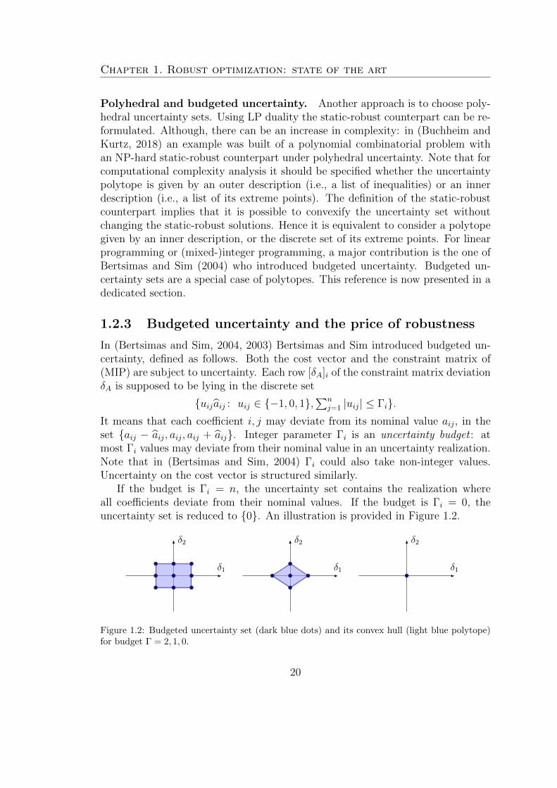
If the budget is Γi = n, the uncertainty set contains the realization whereall coefficients deviate from their nominal values. If the budget is Γi = 0, theuncertainty set is reduced to {0}. An illustration is provided in Figure 1.2.
δ1
δ2
•••
•••
••• δ1
δ2
•••
• •δ1
δ2
•
Figure 1.2: Budgeted uncertainty set (dark blue dots) and its convex hull (light blue polytope)for budget Γ = 2, 1, 0.
20
Chapter 1. Robust optimization: state of the art
Regarding tractability, the authors studied the robust counterpart of an MIPunder budgeted uncertainty. They obtained positive results: the robust counter-part of an MIP under budgeted uncertainty can be reformulated into an MIP, withsize reasonably increased. They also focused on the case of cost uncertainty for acombinatorial problem. If the original problem is polynomial, the robust counter-part can be solved through a polynomial number of calls to an algorithm for theoriginal problem. An approximation algorithm for the original problem also yieldsan approximation algorithm for the robust counterpart. Those results advocatefor the practical implementability of the robust approach, since the robust coun-terpart can be solved with the same tools as those for the deterministic problem(either through an MIP solver, or with a dedicated algorithm).
Bertsimas and Sim defined the price of robustness as the increase of the cost ofa robust solution, compared to the cost of a solution when there is no uncertainty.The uncertainty budget Γ can be used to tune the price of robustness, by chang-ing the number of deviations in the uncertainty set. Budgeted uncertainty is thusappealing because it yields to tractable robust problems, understandable to practi-tioners, and with a parameter Γ to control the price of robustness. Note that theseresults have had a very important influence on the robust optimization literature,and budgeted uncertainty has become a standard uncertainty representation inrobust approaches.
1.2.4 Uncertainty modelling in static robustness
Let us finish with a few remarks on the choice of the uncertainty set in staticrobustness. These remarks carry over to other robust approaches.
When designing uncertainty sets for a robust problem, multiple aspects are tobe taken into account, among which the following.
I First, the relevance of the uncertainty set, in the sense that the uncertaintyset must contain realizations corresponding to what the decision maker wantsto hedge against. This is a qualitative appreciation of whether the uncer-tainty set is convincing. It is also necessary that the parameters defining theuncertainty set (e.g., the range where coefficients lie, the uncertainty budget)can actually be given values by the practitioners.
I The type of the associated robust problem obtained for this uncertainty set:is it a convex program? a linear or integer program? can it be solved withsome generic solver? It is often wanted that the robust counterpart does notdiffer too much from the original problem, i.e., that belongs to the same classof problems (e.g., LPs) and that the overhead computational effort to solveit is not too high.
I The computational complexity of the associated robust problem: is it com-
21
Chapter 1. Robust optimization: state of the art
putationally tractable? Concerning computational complexity, as noted in(Buchheim and Kurtz, 2018), uncertainty sets with very correlated param-eters (e.g., scenarios) lead to difficult problems; uncertainty sets with nocorrelation (e.g., box uncertainty) lead to easy cases.
I Finally, the price of robustness. An important issue of a high price of ro-bustness, in an OR perspective, is that robust solutions that are very costlyare likely to be discarded by decision makers. Thus a control on the price ofrobustness is necessary, to make robust optimization applicable.
1.3 Two-stage robust optimization
Let us now review two-stage and adjustable-robust optimization approaches.
1.3.1 Definition
In the static-robust approach, decisions are made before the uncertainty realizationis observed, and there is no possibility of revising them afterwards. The authors of(Ben-Tal et al., 2004) introduced a new class of robust problems, where decisionsare made along a 2-stage process:
– First-stage decisions, called “here and now” decisions, are made before un-certainty realization is known.
– Second-stage decisions, called “wait and see” decisions, are made after un-certainty realization is known. Second-stage decisions are also called recoursedecisions, or adjustable since they adjust to uncertainty realization.
Such a 2-stage decision process is classical in stochastic optimization, see, e.g.,(Birge and Louveaux, 2011).
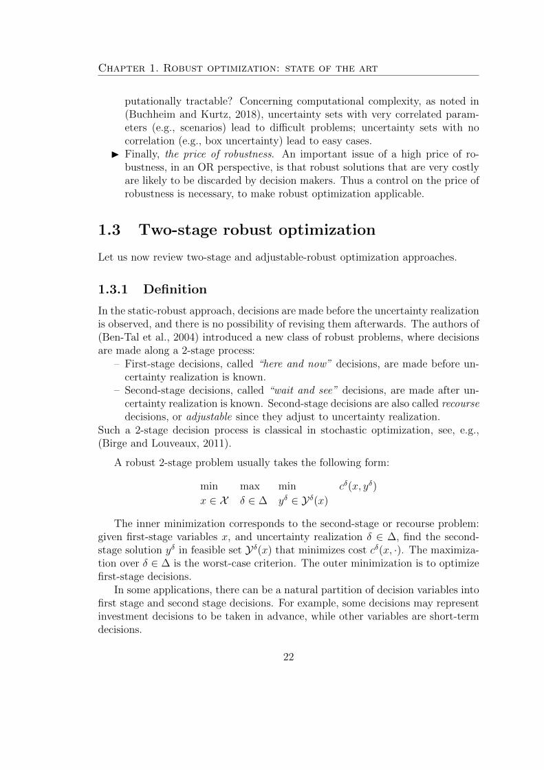
A robust 2-stage problem usually takes the following form:
min max min cδ(x, yδ)
x ∈ X δ ∈ ∆ yδ ∈ Yδ(x)
The inner minimization corresponds to the second-stage or recourse problem:given first-stage variables x, and uncertainty realization δ ∈ ∆, find the second-stage solution yδ in feasible set Yδ(x) that minimizes cost cδ(x, ·). The maximiza-tion over δ ∈ ∆ is the worst-case criterion. The outer minimization is to optimizefirst-stage decisions.
In some applications, there can be a natural partition of decision variables intofirst stage and second stage decisions. For example, some decisions may representinvestment decisions to be taken in advance, while other variables are short-termdecisions.
22
Chapter 1. Robust optimization: state of the art
Importantly, two-stage robust problems are less conservative that their static-robust counterpart. To see this, the two-stage robust problem can be rewrittenwith one variable yδ per realization δ ∈ ∆. Then a solution to the two-stagerobust problem corresponds to x ∈ X and a collection (yδ)δ∈∆ of second-stagesolutions such that yδ ∈ Yδ(x) for every δ ∈ ∆. By contrast, in the static-robustcounterpart the vector y does not depend on δ, and thus y ∈ Yδ(x) for every δ ∈ ∆.Hence the static-robust optimal value is not less than the two-stage robust optimalvalue. The price of robustness is thus decreased, if some variables are allowed tobe adjustable.
An important special case of two-stage problems is the following, where thereare no first-stage variables:
(Adj-P) max min cδ(xδ)
δ ∈ ∆ xδ ∈ X δ
In the sequel, we refer to this problem as the adjustable-robust counterpart ofproblem (P). The value of the adjustable-robust problem is then the worst-casevalue of an optimal solution of the second-stage instance, with feasible set X δ andobjective function cδ. We mention that in the literature, the terms “two-stage”and “adjustable” are often used as synonyms. In this work adjustable-robustnesswill more specifically denote the (Adj-P) problem.
1.3.2 Examples
Let us now illustrate the adjustable-robustness concept on examples for the Se-lection and PERT Scheduling problems.
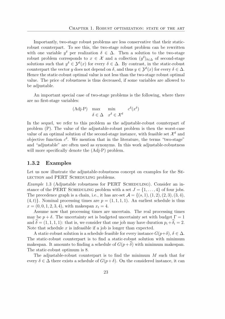
Example 1.3 (Adjustable robustness for PERT Scheduling). Consider an in-stance of the PERT Scheduling problem with a set J = {1, . . . , 4} of four jobs.The precedence graph is a chain, i.e., it has arc-set A = {(s, 1), (1, 2), (2, 3), (3, 4),(4, t)}. Nominal processing times are p = (1, 1, 1, 1). An earliest schedule is thusx = (0, 0, 1, 2, 3, 4), with makespan xt = 4.
Assume now that processing times are uncertain. The real processing timesmay be p+ δ. The uncertainty set is budgeted uncertainty set with budget Γ = 1and δ = (1, 1, 1, 1): that is, we consider that one job may have duration pi+ δi = 2.Note that schedule x is infeasible if a job is longer than expected.
A static-robust solution is a schedule feasible for every instance G(p+δ), δ ∈ ∆.The static-robust counterpart is to find a static-robust solution with minimummakespan. It amounts to finding a schedule of G(p+ δ) with minimum makespan.The static-robust optimum is 8.
The adjustable-robust counterpart is to find the minimum M such that forevery δ ∈ ∆ there exists a schedule of G(p+ δ). On the considered instance, it can
23
Chapter 1. Robust optimization: state of the art
be shown that the optimal value of the adjustable-robust counterpart is 5. Indeed,for any δ ∈ ∆, the earliest schedule of G(p+ δ) has makespan at most 5. It is lessthat the static-robust optimal value of 8.
For general precedence graph the adjustable-robust problem was studied in(Minoux, 2007a,b). It was shown to be solvable in polynomial time for budgeteduncertainty. The algorithm is to compute by dynamic programming, the lengthof all longest paths in the precedence graph where γ ≤ Γ deviations of processingtimes occur. �
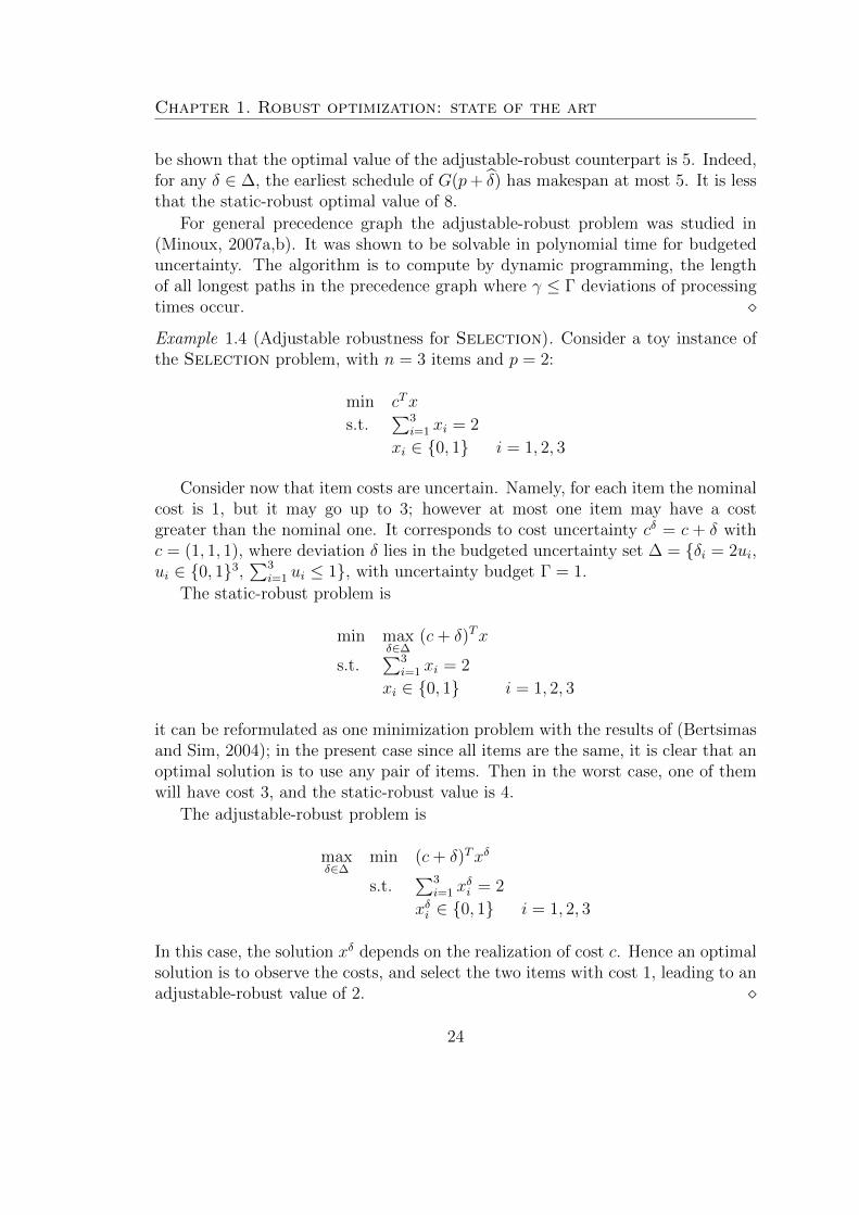
Example 1.4 (Adjustable robustness for Selection). Consider a toy instance ofthe Selection problem, with n = 3 items and p = 2:
min cTx
s.t.∑3
i=1 xi = 2
xi ∈ {0, 1} i = 1, 2, 3
Consider now that item costs are uncertain. Namely, for each item the nominalcost is 1, but it may go up to 3; however at most one item may have a costgreater than the nominal one. It corresponds to cost uncertainty cδ = c + δ withc = (1, 1, 1), where deviation δ lies in the budgeted uncertainty set ∆ = {δi = 2ui,ui ∈ {0, 1}3,
∑3i=1 ui ≤ 1}, with uncertainty budget Γ = 1.
The static-robust problem is
min maxδ∈∆
(c+ δ)Tx
s.t.∑3
i=1 xi = 2
xi ∈ {0, 1} i = 1, 2, 3
it can be reformulated as one minimization problem with the results of (Bertsimasand Sim, 2004); in the present case since all items are the same, it is clear that anoptimal solution is to use any pair of items. Then in the worst case, one of themwill have cost 3, and the static-robust value is 4.
The adjustable-robust problem is
maxδ∈∆
min (c+ δ)Txδ
s.t.∑3
i=1 xδi = 2
xδi ∈ {0, 1} i = 1, 2, 3
In this case, the solution xδ depends on the realization of cost c. Hence an optimalsolution is to observe the costs, and select the two items with cost 1, leading to anadjustable-robust value of 2. �
24
Chapter 1. Robust optimization: state of the art
1.3.3 Computational complexity of robust two-stageproblems
The main challenge associated to 2-stage robust problems is tractability. In (Ben-Tal et al., 2004), it was shown that an adjustable robust problem can be NP-hard,even for a linear program and polyhedral uncertainty set – a case where the staticrobust problem is easy to solve. The authors note that “unfortunately, there isa price to pay for the flexibility of the adjustable-robust counterpart”. Indeed,the decrease of the price of robustness goes hand in hand with an increase of thecomputational complexity.
1.3.3.1 Two-stage approximation approaches
A trend in the literature is thus the design of approximations for two-stage robustproblems that are computationally affordable.
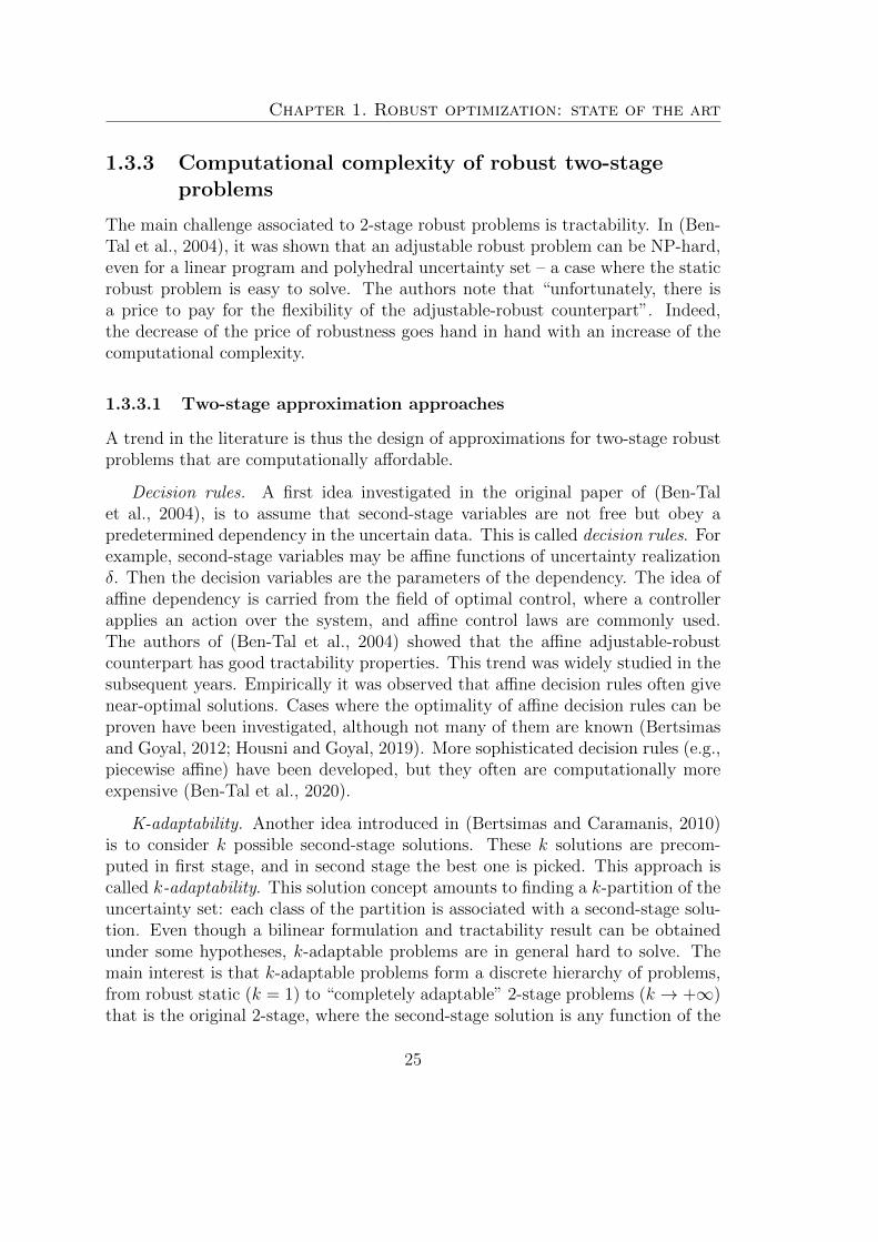
Decision rules. A first idea investigated in the original paper of (Ben-Talet al., 2004), is to assume that second-stage variables are not free but obey apredetermined dependency in the uncertain data. This is called decision rules. Forexample, second-stage variables may be affine functions of uncertainty realizationδ. Then the decision variables are the parameters of the dependency. The idea ofaffine dependency is carried from the field of optimal control, where a controllerapplies an action over the system, and affine control laws are commonly used.The authors of (Ben-Tal et al., 2004) showed that the affine adjustable-robustcounterpart has good tractability properties. This trend was widely studied in thesubsequent years. Empirically it was observed that affine decision rules often givenear-optimal solutions. Cases where the optimality of affine decision rules can beproven have been investigated, although not many of them are known (Bertsimasand Goyal, 2012; Housni and Goyal, 2019). More sophisticated decision rules (e.g.,piecewise affine) have been developed, but they often are computationally moreexpensive (Ben-Tal et al., 2020).
K-adaptability. Another idea introduced in (Bertsimas and Caramanis, 2010)is to consider k possible second-stage solutions. These k solutions are precom-puted in first stage, and in second stage the best one is picked. This approach iscalled k-adaptability. This solution concept amounts to finding a k-partition of theuncertainty set: each class of the partition is associated with a second-stage solu-tion. Even though a bilinear formulation and tractability result can be obtainedunder some hypotheses, k-adaptable problems are in general hard to solve. Themain interest is that k-adaptable problems form a discrete hierarchy of problems,from robust static (k = 1) to “completely adaptable” 2-stage problems (k → +∞)that is the original 2-stage, where the second-stage solution is any function of the
25
Chapter 1. Robust optimization: state of the art
uncertainty. Subsequent work on k-adaptability include, e.g., (Hanasusanto et al.,2015; Subramanyam et al., 2020).
Note that decision rules and k-adaptability are two approximations that arenot comparable (one can be better than another on an instance, and vice versa).
1.3.3.2 Two-stage exact approaches
Another line of research is to design exact approaches to solve 2-stage problems,usually based on decomposition approaches.
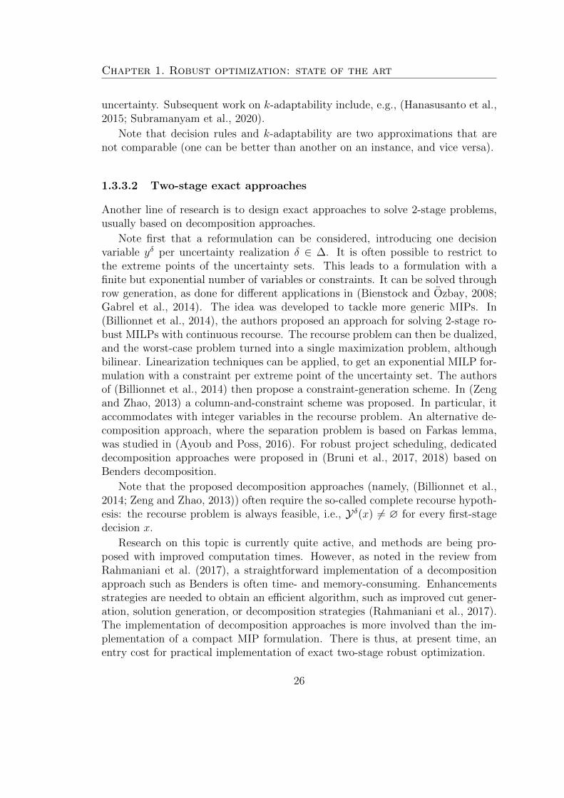
Note first that a reformulation can be considered, introducing one decisionvariable yδ per uncertainty realization δ ∈ ∆. It is often possible to restrict tothe extreme points of the uncertainty sets. This leads to a formulation with afinite but exponential number of variables or constraints. It can be solved throughrow generation, as done for different applications in (Bienstock and Ozbay, 2008;Gabrel et al., 2014). The idea was developed to tackle more generic MIPs. In(Billionnet et al., 2014), the authors proposed an approach for solving 2-stage ro-bust MILPs with continuous recourse. The recourse problem can then be dualized,and the worst-case problem turned into a single maximization problem, althoughbilinear. Linearization techniques can be applied, to get an exponential MILP for-mulation with a constraint per extreme point of the uncertainty set. The authorsof (Billionnet et al., 2014) then propose a constraint-generation scheme. In (Zengand Zhao, 2013) a column-and-constraint scheme was proposed. In particular, itaccommodates with integer variables in the recourse problem. An alternative de-composition approach, where the separation problem is based on Farkas lemma,was studied in (Ayoub and Poss, 2016). For robust project scheduling, dedicateddecomposition approaches were proposed in (Bruni et al., 2017, 2018) based onBenders decomposition.
Note that the proposed decomposition approaches (namely, (Billionnet et al.,2014; Zeng and Zhao, 2013)) often require the so-called complete recourse hypoth-esis: the recourse problem is always feasible, i.e., Yδ(x) 6= ∅ for every first-stagedecision x.
Research on this topic is currently quite active, and methods are being pro-posed with improved computation times. However, as noted in the review fromRahmaniani et al. (2017), a straightforward implementation of a decompositionapproach such as Benders is often time- and memory-consuming. Enhancementsstrategies are needed to obtain an efficient algorithm, such as improved cut gener-ation, solution generation, or decomposition strategies (Rahmaniani et al., 2017).The implementation of decomposition approaches is more involved than the im-plementation of a compact MIP formulation. There is thus, at present time, anentry cost for practical implementation of exact two-stage robust optimization.
26
Chapter 1. Robust optimization: state of the art
1.4 Solution stability in reoptimization and
robust optimization
In this section, we first present a 2-stage decision process, and point out the ques-tion of solution stability arising in this framework. We then review related workon how solution stability can be addressed in both stages, in reoptimization androbust optimization.
1.4.1 A two-stage decision process
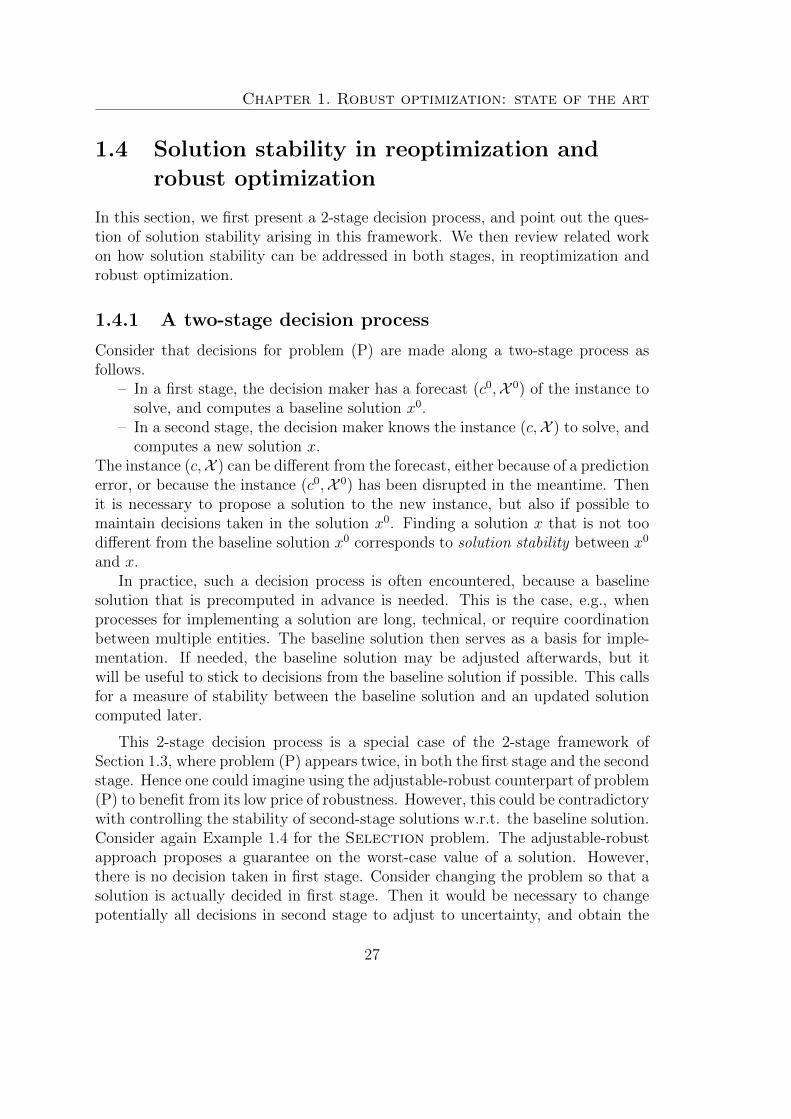
Consider that decisions for problem (P) are made along a two-stage process asfollows.
– In a first stage, the decision maker has a forecast (c0,X 0) of the instance tosolve, and computes a baseline solution x0.
– In a second stage, the decision maker knows the instance (c,X ) to solve, andcomputes a new solution x.
The instance (c,X ) can be different from the forecast, either because of a predictionerror, or because the instance (c0,X 0) has been disrupted in the meantime. Thenit is necessary to propose a solution to the new instance, but also if possible tomaintain decisions taken in the solution x0. Finding a solution x that is not toodifferent from the baseline solution x0 corresponds to solution stability between x0
and x.In practice, such a decision process is often encountered, because a baseline
solution that is precomputed in advance is needed. This is the case, e.g., whenprocesses for implementing a solution are long, technical, or require coordinationbetween multiple entities. The baseline solution then serves as a basis for imple-mentation. If needed, the baseline solution may be adjusted afterwards, but itwill be useful to stick to decisions from the baseline solution if possible. This callsfor a measure of stability between the baseline solution and an updated solutioncomputed later.
This 2-stage decision process is a special case of the 2-stage framework ofSection 1.3, where problem (P) appears twice, in both the first stage and the secondstage. Hence one could imagine using the adjustable-robust counterpart of problem(P) to benefit from its low price of robustness. However, this could be contradictorywith controlling the stability of second-stage solutions w.r.t. the baseline solution.Consider again Example 1.4 for the Selection problem. The adjustable-robustapproach proposes a guarantee on the worst-case value of a solution. However,there is no decision taken in first stage. Consider changing the problem so that asolution is actually decided in first stage. Then it would be necessary to changepotentially all decisions in second stage to adjust to uncertainty, and obtain the
27
Chapter 1. Robust optimization: state of the art
low price of adjustable-robustness. Precisely, in Example 1.4, if an item is selectedin first-stage with no possibility of changing this decision in second stage, thenthe price of robustness equals the static-robust one. That is, there is a trade-offbetween the guarantee of decisions and the price of robustness.
It is thus important in the design of a robust 2-stage approach, to know whethera guarantee on the solution, or on the value of the solution, is needed. Note thatin static robustness, we implicitly obtained a guarantee not only on the value of asolution, but also on the solution itself. This does not hold for 2-stage problems. Inthe project scheduling literature such a choice was emphasized: shall we guaranteethe makespan? or the starting times of the jobs?
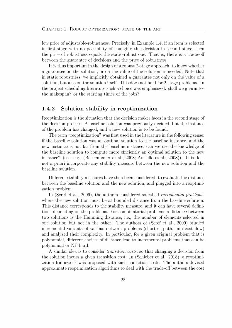
1.4.2 Solution stability in reoptimization
Reoptimization is the situation that the decision maker faces in the second stage ofthe decision process. A baseline solution was previously decided, but the instanceof the problem has changed, and a new solution is to be found.
The term “reoptimization” was first used in the literature in the following sense:if the baseline solution was an optimal solution to the baseline instance, and thenew instance is not far from the baseline instance, can we use the knowledge ofthe baseline solution to compute more efficiently an optimal solution to the newinstance? (see, e.g., (Bockenhauer et al., 2008; Ausiello et al., 2008)). This doesnot a priori incorporate any stability measure between the new solution and thebaseline solution.
Different stability measures have then been considered, to evaluate the distancebetween the baseline solution and the new solution, and plugged into a reoptimi-zation problem.
In (Seref et al., 2009), the authors considered so-called incremental problems,where the new solution must be at bounded distance from the baseline solution.This distance corresponds to the stability measure, and it can have several defini-tions depending on the problems. For combinatorial problems a distance betweentwo solutions is the Hamming distance, i.e., the number of elements selected inone solution but not in the other. The authors of (Seref et al., 2009) studiedincremental variants of various network problems (shortest path, min cost flow)and analyzed their complexity. In particular, for a given original problem that ispolynomial, different choices of distance lead to incremental problems that can bepolynomial or NP-hard.
A similar idea is to consider transition costs, so that changing a decision fromthe solution incurs a given transition cost. In (Schieber et al., 2018), a reoptimi-zation framework was proposed with such transition costs. The authors devisedapproximate reoptimization algorithms to deal with the trade-off between the cost
28
Chapter 1. Robust optimization: state of the art
of the new solution and the total transition cost. Transition costs appear in otherworks such as (Gupta et al., 2014; Bampis et al., 2018) where they are aggregatedwith the cost of the solution into a single objective function.
Reoptimization with a stability measure is also related to bi-objective opti-mization, because of the trade-off between the quality of the solution and thestability measure. Using transition costs as stability measure often leads to opti-mization problems with two linear objectives, the cost of the new solution and thetotal transition cost. Setting one of the criteria as a constraint leads to budgetedoptimization problems, that are in general NP-hard (see, e.g., (Aggarwal et al.,1982) for the budgeted spanning tree problem, (Berger et al., 2011) for budgetedmatching).
For optimization problems with continuous variables, a larger variety of stabil-ity measures can be considered. The distance between solutions can be expressedas a L1-norm, as done in (Nasrabadi and Orlin, 2013) for linear programs.
As for project scheduling problems, a variety of dedicated reoptimization prob-lems were studied. Reoptimization, in that case, is to repair a schedule againstdisruptions, such as disruptions in jobs durations, or the arrival of new jobs to beinserted. This is called reactive scheduling, or rescheduling. An approach to repairschedules is to apply heuristics such as decision rules (Smith, 1995; de Vonderet al., 2007). Such heuristics do not a priori guarantee solution stability, but theymay be applied only on a subset of the schedule, leaving the rest of the scheduleunchanged.
Rescheduling approaches with a stability feature have been proposed, with avariety of criteria. It can be to minimize a continuous deviation measure w.r.t. thebaseline schedule (Sakkout and Wallace, 2000; de Vonder et al., 2007), the cost in-curred when modifying the solution (Deblaere et al., 2011), or a deviation measurebased on the makespan (Artigues and Roubellat, 2000). Another criterion could bethe number of modifications in the schedule (Calhoun et al., 2002; Bendotti et al.,2017). Namely in (Bendotti et al., 2017), the anchoring level was introduced asthe number of identical starting times between two project schedules. Note thatthe literature on exact approaches to reactive scheduling is rather scarce, mostreferences investigate heuristics. For more references on reactive scheduling, werefer to the surveys (Herroelen and Leus, 2002; Hazır and Ulusoy, 2020).
1.4.3 Solution stability in robust optimization
After defining a stability measure and the associated reoptimization problem, aquestion is to compute a baseline solution. This is the problem faced by thedecision maker at first stage.
The first-stage problem can be cast in the framework of robust optimization.
29
Chapter 1. Robust optimization: state of the art
Let us now review related work in the field of robust optimization, where in sec-ond stage the recourse problem incorporates a stability measure. Note that alter-natively, stochastic or multistage models were proposed in the literature, basednamely on transition costs (Gupta et al., 2014; Bampis et al., 2018).
In (Liebchen et al., 2009) the authors introduced the concept of recoverable ro-bustness as a very general framework for robust optimization with limited recourse.The reasons for limited recourse are multiple.
– Practical rules. A first reason is that the recourse should resemble (simple)algorithms that are used in practice for repairing solutions. The authorsprovide an illustration on timetabling for railway applications, where recoursedecisions are, e.g., train delays, or breaking transfers between two trains.
– Tractability. Another reason is tractability: the recourse problem is to besolved quickly, and thus it should be reasonably tractable, or solvable throughsome solver or algorithm.
– Solution stability. The last aspect is solution stability, in the sense that it isgood practice not to change too much the solution in the recourse problem. Inparticular, a recoverable robust approach is to bound the number of changesin the solution.
Recoverable robustness is thus a very broad concept, that need to be instan-tiated on specific problems to be further studied. Recoverable robust railwayapplications were studied in (Liebchen et al., 2009; D’Angelo et al., 2011).
A research line emerged on combinatorial problems where recoverable robust-ness is understood in a more restrictive sense: it corresponds to changing at mostk decisions in the recourse problem. Then recoverable robustness coincides withrobust optimization with incremental recourse proposed in (Nasrabadi and Orlin,2013). The focus was on the computational complexity of recoverable robust vari-ants of famous problems, under standard uncertainty representation such as bud-geted uncertainty. This includes the knapsack problem (Busing et al., 2011), short-est path problems (Busing, 2012), the min cost spanning tree problem (Hradovichet al., 2017), the selection problem (Kasperski and Zielinski, 2017), among others.As noted in the survey (Kasperski and Zielinski, 2016), most of the results on re-coverable robust problems are negative ones. They happen to be very hard, sincethey retain the computational complexity of both the static-robust problem, andthe reoptimization problem. The authors note that the literature is still scarceon approximation algorithms or exact approaches to handle NP-hard recoverablerobust problems.
In the project scheduling literature, a related approach is proactive/reactivescheduling (Herroelen and Leus, 2002). While reactive scheduling corresponds tothe recourse problem, proactive scheduling corresponds to the first-stage problem.The goal is to optimize in a combined way the baseline solution, and the reactive
30
Chapter 1. Robust optimization: state of the art
actions to be taken depending on uncertainty realization. Proactive schedulingproblems including a stochastic continuous stability measure were investigated in(Herroelen and Leus, 2004). However, these problems are relative to stochasticoptimization, and not robust optimization as defined in the present chapter. Theliterature on robustness for project scheduling problems, even without any stabilitymeasure, is scarce, see (Artigues et al., 2013) for a min regret problem, (Minoux,2007b) and (Bruni et al., 2017) for adjustable-robust problems. Even thoughrobust project scheduling problems with a stability feature appear to be of clearinterest for project managers (Hazır and Ulusoy, 2020), they have been barelyaddressed in the literature so far. In (Bendotti et al., 2017), a so-called anchor-proactive problem was proposed. The criterion is a guarantee over the number ofjobs with stable starting times. The problem was proven polynomial under boxuncertainty. The proposed stability criterion is combinatorial, in contrast withmost stability measures studied in project scheduling literature.
In this thesis, we build upon the work of (Bendotti et al., 2017). We proposethe anchoring level as a combinatorial stability measure for discrete optimizationproblems, and anchored solutions as a concept for stability in robust optimization.The generic concepts of the thesis are exposed in Chapter 2.
31

Chapter 1. Robust optimization: state of the art
32
Chapter 2
Anchored solutions: concepts
In this chapter we present the general concepts of anchored solutions, in the frame-work of the 2-stage decision process described in Section 1.4 of Chapter 1.
In Section 2.1 we first introduce the anchoring level as a criterion to countthe number of identical decisions between a baseline solution and a new solutionof optimization problem (P). In Section 2.2 we introduce anchor-reoptimizationproblems, that are arising in second stage to compute the new solution. In Sec-tion 2.3 we define anchor-robust problems. These are the robust problems facedin first stage to compute a baseline solution along with a guarantee on a subset ofbaseline decisions.
Problems defined in this chapter are posed in generic form. They are instanti-ated and studied in more details in Part II for combinatorial problems, and Part IIIfor project scheduling problems.
2.1 Anchoring level
Let us first introduce the anchoring level, to serve as a stability measure in reopti-mization and robust optimization. Recall that S denotes the space where decisionvariables lie, e.g., S = {0, 1}I for binary variables, S = RI for continuous variables.Given two vectors x, y ∈ S, let the anchoring level be defined as
σ(x, y) = |{i ∈ I : xi = yi}|.
Since coordinates of vectors x and y correspond to decisions, the anchoring levelis the number of decisions that are identical in x and y. Note also that σ(x, y) =|I| − d(x, y) where d(x, y) is the Hamming distance between vectors x an y. Theanchoring level was coined as such in (Bendotti et al., 2017) where it was introducedas a stability measure for reoptimization in project scheduling.
33
Chapter 2. Anchored solutions: concepts
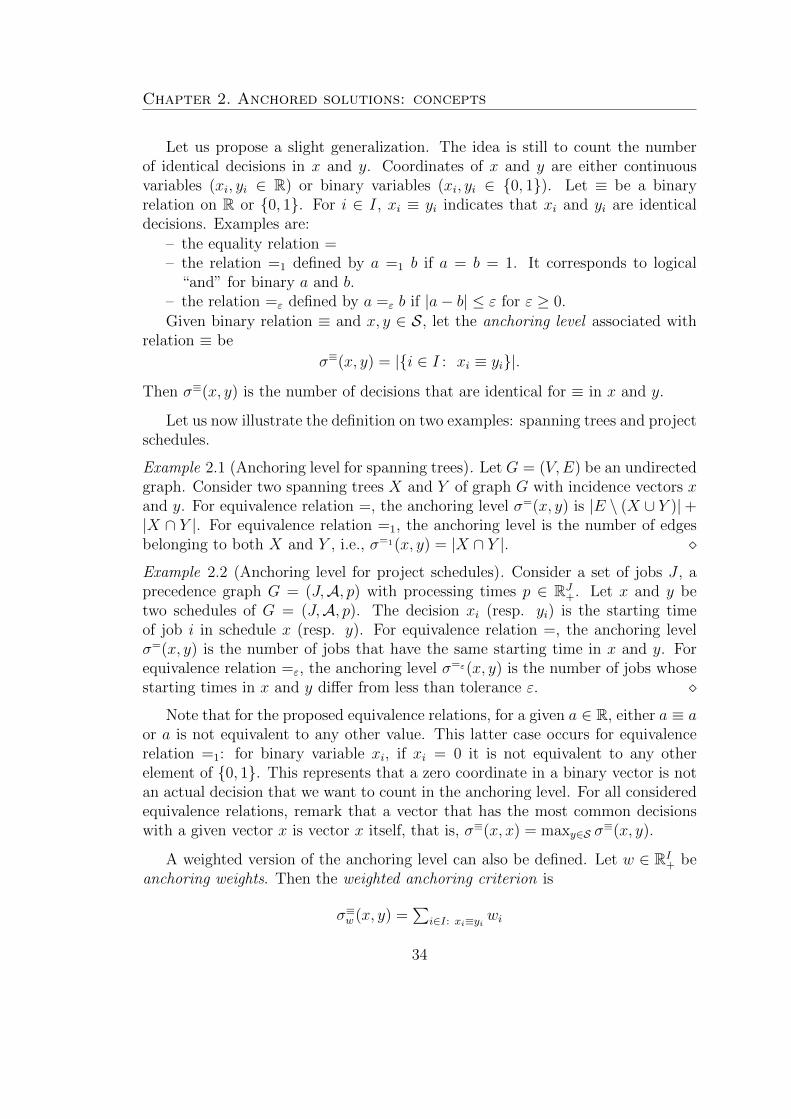
Let us propose a slight generalization. The idea is still to count the numberof identical decisions in x and y. Coordinates of x and y are either continuousvariables (xi, yi ∈ R) or binary variables (xi, yi ∈ {0, 1}). Let ≡ be a binaryrelation on R or {0, 1}. For i ∈ I, xi ≡ yi indicates that xi and yi are identicaldecisions. Examples are:
– the equality relation =– the relation =1 defined by a =1 b if a = b = 1. It corresponds to logical
“and” for binary a and b.– the relation =ε defined by a =ε b if |a− b| ≤ ε for ε ≥ 0.Given binary relation ≡ and x, y ∈ S, let the anchoring level associated with
relation ≡ be
σ≡(x, y) = |{i ∈ I : xi ≡ yi}|.
Then σ≡(x, y) is the number of decisions that are identical for ≡ in x and y.
Let us now illustrate the definition on two examples: spanning trees and projectschedules.
Example 2.1 (Anchoring level for spanning trees). Let G = (V,E) be an undirectedgraph. Consider two spanning trees X and Y of graph G with incidence vectors xand y. For equivalence relation =, the anchoring level σ=(x, y) is |E \ (X ∪ Y )|+|X ∩ Y |. For equivalence relation =1, the anchoring level is the number of edgesbelonging to both X and Y , i.e., σ=1(x, y) = |X ∩ Y |. �
Example 2.2 (Anchoring level for project schedules). Consider a set of jobs J , aprecedence graph G = (J,A, p) with processing times p ∈ RJ
+. Let x and y betwo schedules of G = (J,A, p). The decision xi (resp. yi) is the starting timeof job i in schedule x (resp. y). For equivalence relation =, the anchoring levelσ=(x, y) is the number of jobs that have the same starting time in x and y. Forequivalence relation =ε, the anchoring level σ=ε(x, y) is the number of jobs whosestarting times in x and y differ from less than tolerance ε. �
Note that for the proposed equivalence relations, for a given a ∈ R, either a ≡ aor a is not equivalent to any other value. This latter case occurs for equivalencerelation =1: for binary variable xi, if xi = 0 it is not equivalent to any otherelement of {0, 1}. This represents that a zero coordinate in a binary vector is notan actual decision that we want to count in the anchoring level. For all consideredequivalence relations, remark that a vector that has the most common decisionswith a given vector x is vector x itself, that is, σ≡(x, x) = maxy∈S σ
≡(x, y).
A weighted version of the anchoring level can also be defined. Let w ∈ RI+ be
anchoring weights. Then the weighted anchoring criterion is
σ≡w (x, y) =∑
i∈I: xi≡yi wi
34
Chapter 2. Anchored solutions: concepts
and clearly σ≡1 (x, y) = σ≡(x, y) with 1 the all-ones vector of RI . The anchoringweight wi is a value representing the benefit of having an identical decision i intwo solutions.
In this chapter, unless specified, we will consider the anchoring level:
– for combinatorial problems (S = {0, 1}I), σ(x, y) = {i ∈ I : xi =1 yi}– for linear programs (S = RI), σ(x, y) = {i ∈ I : xi = yi}.
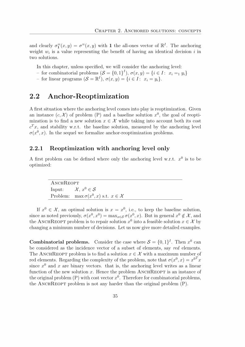
2.2 Anchor-Reoptimization
A first situation where the anchoring level comes into play is reoptimization. Givenan instance (c,X ) of problem (P) and a baseline solution x0, the goal of reopti-mization is to find a new solution x ∈ X while taking into account both its costcTx, and stability w.r.t. the baseline solution, measured by the anchoring levelσ(x0, x). In the sequel we formalize anchor-reoptimization problems.
2.2.1 Reoptimization with anchoring level only
A first problem can be defined where only the anchoring level w.r.t. x0 is to beoptimized:
AnchReopt
Input: X , x0 ∈ SProblem: maxσ(x0, x) s.t. x ∈ X
If x0 ∈ X , an optimal solution is x = x0, i.e., to keep the baseline solution,since as noted previously, σ(x0, x0) = maxx∈S σ(x0, x). But in general x0 /∈ X , andthe AnchReopt problem is to repair solution x0 into a feasible solution x ∈ X bychanging a minimum number of decisions. Let us now give more detailed examples.
Combinatorial problems. Consider the case where S = {0, 1}I . Then x0 canbe considered as the incidence vector of a subset of elements, say red elements.The AnchReopt problem is to find a solution x ∈ X with a maximum number ofred elements. Regarding the complexity of the problem, note that σ(x0, x) = x0Txsince x0 and x are binary vectors. that is, the anchoring level writes as a linearfunction of the new solution x. Hence the problem AnchReopt is an instance ofthe original problem (P) with cost vector x0. Therefore for combinatorial problems,the AnchReopt problem is not any harder than the original problem (P).
35
Chapter 2. Anchored solutions: concepts
Linear programming. Consider the case where S = RI , and X is the polyhe-dron {x ∈ RI : x ≥ 0, Ax ≤ b}. Let x0 ∈ RI . Note that by contrast with combi-natorial problems, the anchoring criterion σ(x0, x) = |{i ∈ I : x0
i = xi}| is not alinear function of the new solution x. We now prove that anchor-reoptimization isNP-hard in that case.
Proposition 2.1. AnchReopt is strongly NP-hard for linear programs.
Proof. The proof is a reduction from the Stable Set problem: given a graphG = (V,E), integer k, is there a stable set U ⊆ V of size |U | ≥ k? Let G = (V,E)be a graph, k ∈ N. Consider the polyhedron X = {x ∈ RV
+ : x ∈ [0, 1]V , xi +xj ≤1 ∀(i, j) ∈ E} and the solution x0 ∈ RV defined by x0
v = 1 for every v ∈ V . Thenσ(x0, x) = |{v ∈ V : xv = 1}|. If there exists a stable set U ⊆ V of size ≥ k, thenits incidence vector χU is in X and σ(x0, χU) ≥ k. Conversely, assume there existsx∗ ∈ X such that σ(x0, x∗) ≥ k. Vector x∗ is not an integer vector, but it hasmore than k coordinates equal to one. Let U = {v ∈ V : x∗v = 1}. Then χU ≤ x∗
and χU ∈ X ∩ {0, 1}V . Hence U is a stable set of size ≥ k. This proves that thedecision version of AnchReopt is strongly NP-complete.
The underlying idea is that the anchoring level is a combinatorial criterion: aredecisions equal or not? When the variables of the original problem are continuous,there can be an increase in complexity induced by the anchoring level, when solvingthe AnchReopt problem.
Project scheduling. In project scheduling, the variables are the starting timesof jobs, which are continuous. In particular PERT Scheduling writes as alinear program. In Chapter 5 we will study cases where AnchReopt can besolved in polynomial time, in contrast with the general NP-hardness result ofProposition 2.1.
Remark that in the definition of AnchReopt, the baseline solution x0 is givenin the input, but the baseline instance X 0 is not. Hence x0 can be any element ofthe space S. For the problems where we study anchor-reoptimization into detail,we were able to obtain polynomiality results for any x0 ∈ S: in particular formatroid bases (Chapter 3) and project scheduling problems (Chapter 5). We didnot require any further properties on x0.
2.2.2 Extendable sets in reoptimization
Let us have a closer look to a decision problem related to AnchReopt, arisingwhen x0 /∈ X .
36
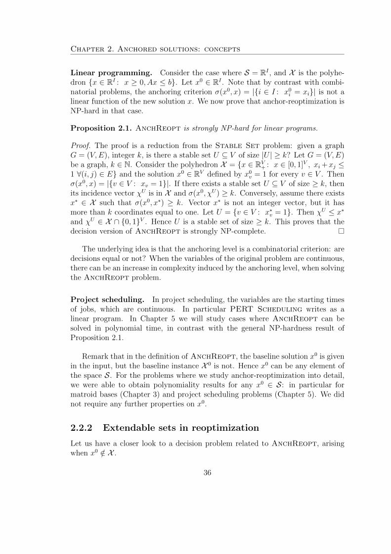
Chapter 2. Anchored solutions: concepts
Extendability
Input: X , x0 ∈ S, H ⊆ I
Question: Is there x ∈ X such that x0i ≡ xi ∀i ∈ H?
The problem is to decide if a subset of decisions (x0i )i∈H from x0 can be extended
into a new feasible solution x ∈ X . Let us say that set H is extendable if theinstance of Extendability problem has answer ‘yes’. The problem AnchReoptis to find an extendable set H of maximum size.
Combinatorial problems. Note that for combinatorial problem, Extendabil-ity is not any harder than the original problem. Setting anchoring weights wi = 1if i ∈ H, and wi = 0 otherwise, it comes that H is extendable if and only ifAnchReopt for anchoring weights w has optimal value at least |H|.
Linear programming. Note that for LPs, Extendability is solvable in poly-nomial time because it writes as an LP with additional equality constraints x0
i = xifor every i ∈ H. Hence deciding if a set is extendable is polynomial, but findingone of maximum size is hard (Proposition 2.1).
Project scheduling. The Extendability problem is studied in Chapter 5 anda combinatorial characterization of extendable sets is provided. This characteriza-tion will be an important building block of the robust approaches proposed next,e.g., in Chapter 6.
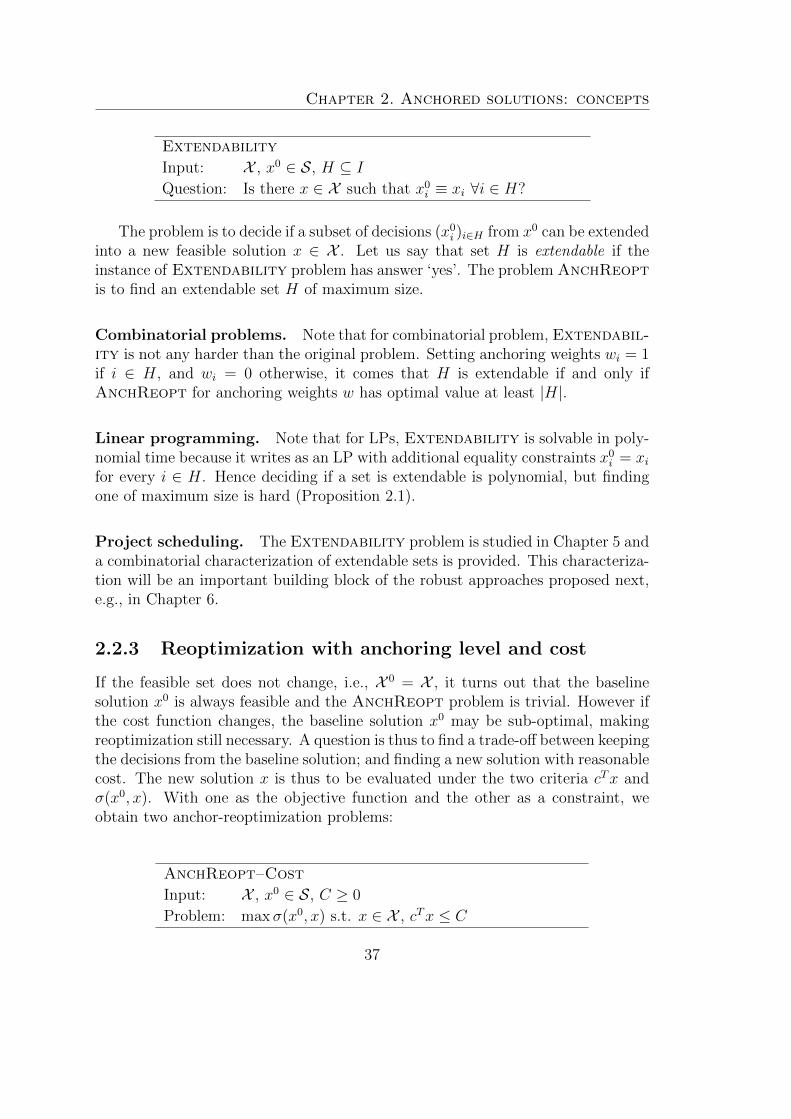
2.2.3 Reoptimization with anchoring level and cost
If the feasible set does not change, i.e., X 0 = X , it turns out that the baselinesolution x0 is always feasible and the AnchReopt problem is trivial. However ifthe cost function changes, the baseline solution x0 may be sub-optimal, makingreoptimization still necessary. A question is thus to find a trade-off between keepingthe decisions from the baseline solution; and finding a new solution with reasonablecost. The new solution x is thus to be evaluated under the two criteria cTx andσ(x0, x). With one as the objective function and the other as a constraint, weobtain two anchor-reoptimization problems:
AnchReopt–Cost
Input: X , x0 ∈ S, C ≥ 0
Problem: maxσ(x0, x) s.t. x ∈ X , cTx ≤ C
37
Chapter 2. Anchored solutions: concepts
AnchReopt–Anch
Input: X , x0 ∈ S, A ∈ NProblem: min cTx s.t. x ∈ X , σ(x0, x) ≥ A
Note that in decision version, both lead to the same decision problem:
Dec-AnchReopt-Anch&Cost
Input: X , x0 ∈ S, C ≥ 0, A ∈ NQuestion: Is there x ∈ X such that cTx ≤ C and σ(x0, x) ≥
A?
Combinatorial problems. For combinatorial problems, these problems will bediscussed in Chapter 3, with a specific focus on the problem of finding a max-weightbasis in a matroid.
Linear programming. Note that for linear programs, AnchReopt–Cost isharder than AnchReopt which was shown to be NP-hard in Section 2.2.1.
Project scheduling. For project scheduling, we obtained that the AnchRe-opt–Cost is polynomial, as for the AnchReopt problem: see Chapter 5.
2.2.4 Restricted reoptimization for NP-hard problems
Let us now present an additional concept to handle an NP-hard original problem(P). Similarly to what was noted in (Liebchen et al., 2009), it is useful to de-sign reoptimization problems that are computationally easy, so that they can beintegrated as the recourse problem of robust 2-stage approaches. In the anchor-reoptimization problems proposed in Section 2.2.1 and Section 2.2.3, the new so-lution x is sought in the feasible set X . In general these problems retain the wholecomplexity of the original problem (P), and thus are NP-hard whenever (P) isNP-hard.
An approach is to consider that only a subset of variables describing the so-lution can be re-optimized. Consider that feasible solutions of problem (P) arerepresented not only with the decision vector x, but also with some additionalvariables φ ∈ RJ . Then a feasible solution is (x, φ) ∈ X . Given a baseline solution(x0, φ), restricted reoptimization is to search for a second-stage solution (x, φ) ∈ X .The φ variables are thus forced to be the same in the baseline solution and thesecond-stage solution. The anchoring level is still evaluated between vectors x0
and x.
38
Chapter 2. Anchored solutions: concepts
Variables φ may capture the structure of the solution: then the second-stagesolution (x, φ) keeps the same structure as the baseline solution (x0, φ). Restrictedreoptimization may be computationally attractive, since it is not necessary to re-optimize the φ variables. Note that it corresponds, in a robust 2-stage perspective,to decide that variables φ are first-stage variables. The recourse problem is thento re-optimize only x variables.
Combinatorial problems. In the present work, we consider only original com-binatorial problems that are solvable in polynomial time. The investigation ofrestricted anchor-reoptimization for combinatorial problems would be an interest-ing research perspective, especially to deal with NP-hard graph problems.
Project scheduling. An example of restricted reoptimization is considered inChapter 5 for the Resource-Constrained Project Scheduling Problem (RCPSP),which is NP-hard and computationally demanding. Variables φ then correspond tosequencing decisions related to resource allocations, while x variables are startingtimes. It is used in Chapter 7 to design efficient robust approaches for the RCPSP.
2.3 Anchor-Robust optimization
Let us now present a robust optimization approach including an anchoring crite-rion, to compute a baseline solution.
2.3.1 Framework
Let us first present the general framework with the chosen uncertainty represen-tation, then recall robust approaches from the literature.
In first stage, the baseline instance is (c0,X 0). In second stage, the new in-stance is (cδ, Xδ). We consider that the baseline instance corresponds to the nom-inal instance of problem (P). We assume, as in the robust optimization paradigmpresented in Chapter 1, that we want to hedge against second-stage instances(cδ,X δ)δ∈∆, with ∆ the uncertainty set. It is assumed that X δ 6= ∅ for everyδ ∈ ∆, i.e., all second-stage instances admit a feasible solution. The baselinesolution x0 is a first-stage decision, while the new solution xδ is a second-stagedecision, adjustable to uncertainty realization δ.
Let us now formally recall static-robust and adjustable-robust approaches fromthe literature, within this framework. These two approaches correspond to twoextreme situations where all variables are in first stage (for static-robustness) orall variables are in second stage (for adjustable-robustness).
The static-robust problem associated with (P) , as stated in Chapter 1, is
39
Chapter 2. Anchored solutions: concepts
(SR-P) min maxδ∈∆
cδTx0
s.t. x0 ∈ X δ ∀δ ∈ ∆
The solution x0 is the baseline solution, chosen before uncertainty realization.There is no explicit second-stage solution; implicitly, xδ = x0 for every δ ∈ ∆.
(SR-P) is overly conservative because of the worst-case cost maxδ∈∆
cδTx0, and the
constraint that x0 is feasible for every second-stage instance. It might even be thatno such static-robust solution exists if ∩δ∈∆X δ = ∅.
The adjustable-robust counterpart of (P) involves one second-stage solution xδ
for every δ ∈ ∆ and it writes
(Adj-P) max min cδTxδ
δ ∈ ∆ s.t. xδ ∈ X δ
In this case, there is no explicit baseline solution x0 in the optimization problem.
2.3.2 Anchored solutions
Let us now introduce an important concept of the thesis, which is the definitionof anchored sets and anchored solutions.
Definition 2.1 (Anchored set). For given ∆, a subset H ⊆ I of decisions isanchored w.r.t. a solution x0 ∈ X 0 if for every δ ∈ ∆, there exists xδ ∈ X δ suchthat x0
i ≡ xδi for every i ∈ H.
An anchored set is thus a subset of decisions from solution x0 that can be,in some sense, guaranteed, since it is always possible to repair x0 into a feasiblesecond-stage solution xδ without changing the decisions x0
i , i ∈ H from the an-chored set. The fact that a decision is unchanged is represented by equivalencerelation ≡.
Let us now define an anchored solution.
Definition 2.2 (Anchored solution). For given ∆, an anchored solution is a pair(x0, H) where x0 ∈ X 0 is a baseline solution and H ⊆ I is anchored w.r.t. x0.
Hence an anchored solution is a baseline solution x0 for problem (P), with aguarantee on decisions of the anchored set H against uncertainty ∆.
Alternatively, we may give an anchored solution as a triplet (x0, H, (xδ)δ∈∆),where x0 ∈ X 0, xδ ∈ X δ for every δ ∈ ∆, and x0
i ≡ xδi for every i ∈ H, δ ∈ ∆. Foran anchored solution given as a pair (x0, H) the existence of second-stage solutionssuch that x0
i = xδi for every i ∈ H, is granted. It may be useful to give explicitly thesecond-stage solutions in the anchored solutions, e.g., to evaluate the worst-casecost of second-stage solutions.
40
Chapter 2. Anchored solutions: concepts
Let us now point out the connection with solutions of the static-robust andadjustable-robust approaches.
Observation 2.1 (Static means all anchored). A solution x0 is static-robust ifand only if all decisions are anchored w.r.t. x0, that is, H = {i ∈ I : x0
i ≡ x0i }.
Note that the set {i ∈ I : x0i ≡ x0
i } is simply I for equivalence relations =and =ε; it is {i ∈ I : x0
i = 1} for binary x and equivalence relation =1.
Observation 2.2 (Adjustable means none anchored). A solution (xδ)δ∈∆ of theadjustable-robust problem corresponds to an anchored solution with H = ∅.
In a solution (xδ)δ∈∆ of the adjustable-robust problem, it may be that somedecisions coincide for every δ ∈ ∆. But since there is no a priori guarantee of that,these are not anchored decisions.
For anchored solutions, criteria of interest are:– cost of the baseline solution c0Tx0
– worst-case cost of second-stage solutions maxδ∈∆ cδTxδ
– size (or weight) of the anchored setThese criteria are conflicting. Namely, optimizing the size of the anchored set leadsto a static-robust solution by Observation 2.1; optimizing the worst-case cost leadsto an adjustable-robust solution by Observation 2.2.
We propose anchored solutions as a middle ground between static-robust andadjustable-robust solutions. Let us illustrate the difference between static-robust,adjustable-robust and anchored solutions on an example.
Example 2.3 (Anchored solutions). Consider the Selection problem with a set Iof n items available. Assume that all items are the same, with nominal cost ci = cfor every i ∈ I. The problem is to select p items among n with minimum totalcost. Consider budgeted uncertainty with budget Γ and deviation δi = 1 for everyi ∈ I. Note that all items play the same role.
A static-robust solution is to select any p items. Then the worst-case cost ofthis solution is attained when deviations occur on the selected items, leading to acost of CostStat(n, p,Γ) = pc+ min{Γ, p}.
In an adjustable-robust solution, the selected items depend on the uncertaintyrealization. An optimal solution is to select items among the ones with no costdeviations (min{p, n−Γ} such items can be selected) then to complete the solutionif necessary with items with cost deviation. This leads to a worst-case cost ofCostAdj(n, p,Γ) = pc+ p−min{p, n− Γ} = pc+ max{0, p− n+ Γ}.
An anchored solution is formed by a first-stage selection x0 and a set of k itemswhich is anchored (with k ≤ p). These anchored items remain in the second-stage solution. What is the worst-case cost of such a solution? The worst-case
41
Chapter 2. Anchored solutions: concepts
uncertainty realization is when the k anchored items have a cost deviation, leadingto a cost of kc+ min{Γ, k}. Then the p− k other items may be changed: in thatsense, the non-anchored items can be selected as in an adjustable-robust solution.It leads to a cost CostAdj(n− k, p− k,Γ−min{Γ, k}) for the non-anchored items.The total cost is CostkAnch(n, p,Γ) = pc+ max{min{Γ, k}, p− n+ Γ}.
It is then clear that CostAdj(n, p,Γ) = Cost0Anch(n, p,Γ) ≤ CostkAnch(n, p,Γ) ≤CostpAnch(n, p,Γ) = CostStat(n, p,Γ) for any number k of anchored items. �
Throughout the thesis, we will illustrate that anchored solutions bridge thegap between static-robustness and adjustable-robustness, see, e.g., Chapter 4 orChapter 6.
2.3.3 Anchor-Robust optimization problems
Let us now formulate robust problems involving anchored solutions. The abovementioned criteria are conflicting: namely, the costs versus the size of the anchoredset. Similarly to anchor-reoptimization, we now define variants, depending onwhether the objective function is to optimize the cost of solutions or the size ofthe anchored set.
Anchored set maximization variant. A first problem is to optimize thesize of the anchored set, while looking for a baseline solution with bounded cost.Let C0 ≥ 0. The Anchor-Robust (AnchRob) problem is
(AnchRob) max |H|x0 ∈ X 0
c0Tx0 ≤ C0
H ⊆ I anchored w.r.t. x0
(AnchRob) can be seen as a robust 2-stage optimization problem. Let us writethe problem under the following form:
max min max |H|x0 ∈ X 0 δ ∈ ∆ xδ ∈ X δ
c0Tx0 ≤ C0 x0i = xδi ∀i ∈ H
H ⊆ I
The recourse problem is then an instance of the Extendability problem:given x0, H ⊆ I and X δ, decide the existence of xδ ∈ X δ such that x0
i = xδi∀i ∈ H. It is only a feasibility problem since the cost |H| does not depend onsecond-stage variables. Hence the inner min/max problem has finite value |H| ifset H is anchored, and infinite value otherwise.
42
Chapter 2. Anchored solutions: concepts
Importantly, (AnchRob) outputs a static-robust solution x0 with H = I if there
exists one respecting the baseline cost condition c0Tx0 ≤ C0. If no static-robustsolution with such a cost exists, an optimal solution of (AnchRob) has a max-sizesubset of anchored jobs H ( I. Note that the condition on the baseline cost couldbe replaced by a condition on the worst-case cost of second-stage solutions.
The Anchor-Robust problem under this Anchored set maximization variantis well-suited for problems with uncertainty on the feasible set. It is studied forproject scheduling under precedence constraints in Chapter 6, Chapter 8, and forthe Resource-Constrained Project Scheduling Problem in Chapter 7.
Worst-case cost minimization. Let us now propose a cost minimizationvariant, which is particularly adapted to the case with cost uncertainty only. Letk ∈ {0, . . . , |I|} be an integer. The problem is to minimize the worst-case cost ofsecond-stage solutions, while ensuring that the anchored set has size at least k.
(AnchRob) min max min cδTxδ
x0 ∈ X 0 δ ∈ ∆ xδ ∈ X δ
H ⊆ I x0i = xδi ∀i ∈ H
|H| ≥ k
In this case the problem clearly writes as a robust 2-stage problem. The set His anchored w.r.t. x0 as soon as the inner max/min has a finite value.
The Anchor-Robust under this worst-case cost minimization variant is studiedfor combinatorial problems with cost uncertainty in Chapter 4.
2.3.4 Connection with recoverable robustness
The concepts of anchor-robustness and recoverable robustness (Liebchen et al.,2009) are closely related, as both are 2-stage concepts with a feature to ensurethat first-stage and second-stage solutions are similar.
Solutions of the recoverable robust approach are formed with a baseline so-lution x0 and a collection (xδ)δ∈∆ of second-stage solutions. For a given integerk ∈ {0, . . . , |I|} a recoverable robust approach is to impose a lower bound on thenumber of common decisions in x0 and xδ. Formally, for every δ ∈ ∆, it is imposedthat |{i ∈ I : x0
i ≡ xδi}| ≥ k, or equivalently, σ(x0, xδ) ≥ k.
Let us now highlight the difference between anchor-robustness and recover-able robustness. Consider a baseline solution x0 and a collection of second-stagesolutions (xδ)δ∈∆.
– x0 and (xδ)δ∈∆ form a recoverable robust solution if for every δ ∈ ∆, thereexists a Hδ such that |Hδ| ≥ k and x0
i ≡ xδi for every i ∈ Hδ.
43
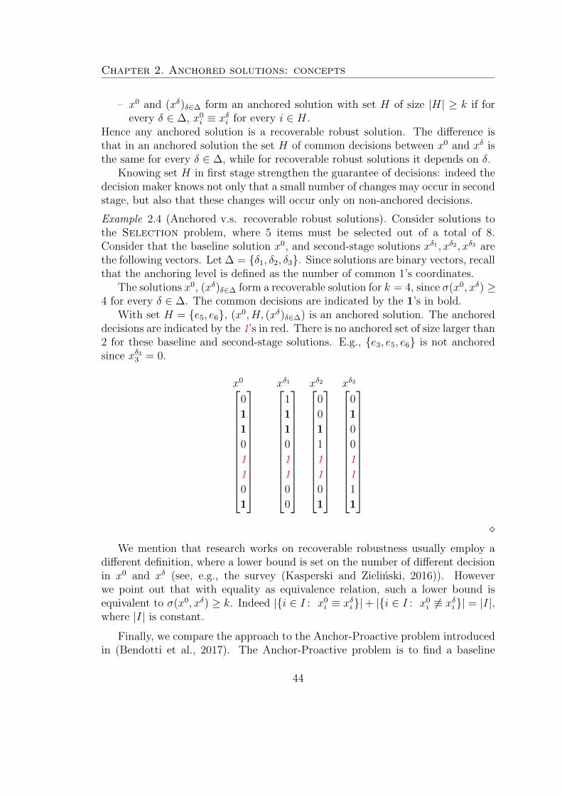
Chapter 2. Anchored solutions: concepts
– x0 and (xδ)δ∈∆ form an anchored solution with set H of size |H| ≥ k if forevery δ ∈ ∆, x0
i ≡ xδi for every i ∈ H.Hence any anchored solution is a recoverable robust solution. The difference isthat in an anchored solution the set H of common decisions between x0 and xδ isthe same for every δ ∈ ∆, while for recoverable robust solutions it depends on δ.
Knowing set H in first stage strengthen the guarantee of decisions: indeed thedecision maker knows not only that a small number of changes may occur in secondstage, but also that these changes will occur only on non-anchored decisions.
Example 2.4 (Anchored v.s. recoverable robust solutions). Consider solutions tothe Selection problem, where 5 items must be selected out of a total of 8.Consider that the baseline solution x0, and second-stage solutions xδ1 , xδ2 , xδ3 arethe following vectors. Let ∆ = {δ1, δ2, δ3}. Since solutions are binary vectors, recallthat the anchoring level is defined as the number of common 1’s coordinates.
The solutions x0, (xδ)δ∈∆ form a recoverable solution for k = 4, since σ(x0, xδ) ≥4 for every δ ∈ ∆. The common decisions are indicated by the 1’s in bold.
With set H = {e5, e6}, (x0, H, (xδ)δ∈∆) is an anchored solution. The anchoreddecisions are indicated by the 1’s in red. There is no anchored set of size larger than2 for these baseline and second-stage solutions. E.g., {e3, e5, e6} is not anchoredsince xδ33 = 0.
x0 xδ1 xδ2 xδ3
0
1
1
0
1
1
0
1
1
1
1
0
1
1
0
0
0
0
1
1
1
1
0
1
0
1
0
0
1
1
1
1
�
We mention that research works on recoverable robustness usually employ adifferent definition, where a lower bound is set on the number of different decisionin x0 and xδ (see, e.g., the survey (Kasperski and Zielinski, 2016)). Howeverwe point out that with equality as equivalence relation, such a lower bound isequivalent to σ(x0, xδ) ≥ k. Indeed |{i ∈ I : x0
i ≡ xδi}|+ |{i ∈ I : x0i 6≡ xδi}| = |I|,
where |I| is constant.
Finally, we compare the approach to the Anchor-Proactive problem introducedin (Bendotti et al., 2017). The Anchor-Proactive problem is to find a baseline
44
Chapter 2. Anchored solutions: concepts
solution x0 ∈ X 0 such that c0Tx0 ≤ C0, maximizing minδ∈∆ maxxδ∈X δ σ(x0, xδ).An anchor-proactive solution with objective value k is thus (x0, (xδ)δ∈∆) such thatfor every δ ∈ ∆, σ(x0, xδ) ≥ k. Introducing set Hδ of common decisions, thiswrites: for every δ ∈ ∆, there exists Hδ such that |Hδ| ≥ k and x0
i ≡ xδi forevery i ∈ Hδ. Thus anchor-proactive solutions corresponds exactly to recoverablesolutions, as previously defined. The difference between the Anchor-Proactiveproblem and recoverable robust problems is mainly the choice of the criterion: inthe former the parameter k is maximized while the baseline cost is bounded, in thelatter the solution cost is minimized for fixed parameter k. These problems arethus variants, similarly to the two variants of the Anchor-Robust problem definedin Section 2.3.
2.3.5 Uncertainty with a worst-case element
All problems were introduced without making any assumption on the structureand properties of the uncertainty. Let us now have a look at the case where theuncertainty set has a so-called worst-case element. This situation is commonlyencountered for simple uncertainty sets, and we will show that anchored solutionshave a specific form in that case. The worst-case element is formally defined asfollows.
Definition 2.3 (Worst-case element of uncertainty set). Let δ+ ∈ ∆. Then δ+ isa worst-case element of the uncertainty set ∆ if X δ+ ⊆ X δ for every δ ∈ ∆ andcδ
+ ≥ cδ for every δ ∈ ∆.
In the sequel, we use the shorthand notation c+ = cδ+
, x+ = xδ+
, X+ = X δ+.
Note that the definition of the worst-case element implies X+ ⊆⋂δ∈∆X δ and
X+ is unique. A simple uncertainty set with a worst-case element is a box. Forexample with cδ = c+ δ and δ ∈ ∆ = Πi∈I [δ
−i , δ
+i ], it comes that δ+ is a worst-case
element of ∆.
Proposition 2.2. Assume the uncertainty set ∆ has a worst-case δ+. Then asolution (x0, H) is anchored for set ∆ if and only if it is anchored for set {δ+}.
Proof. Since {δ+} ⊆ ∆, it is clear that if (x0, H) is anchored for ∆, it is anchoredfor the subset {δ+}. Conversely, assume there exists x+ ∈ X+ such that x0
i = x+i
for every i ∈ H. This solution x+ is thus in X δ for every δ ∈ ∆ by assumption onthe worst-case element. Hence (x0, H) is anchored for ∆.
This observation can be interpreted as a dominance of the worst-case elementin the uncertainty set. Then the Anchor-Robust optimization problems can besimplified into one-level optimization problems. For example for the Anchored setmaximization variant, with Proposition 2.2 the condition H anchored w.r.t. x0 for
45
Chapter 2. Anchored solutions: concepts
set ∆ reduces to the existence of x+ ∈ X+ such that x0i = x+
i for every i ∈ H+.Hence the (AnchRob) problem is
max |H+|s.t. x0 ∈ X 0
c0Tx0 ≤ C0
x+ ∈ X+
x0i = x+
i ∀i ∈ H+
This problem is studied, e.g., in Section 6.4.1 for anchor-robust project scheduling.Consider now the worst-case cost minimization variant. Consider an anchored
solution (x0, H, (xδ)δ∈∆) where every xδ is an optimal solution to the recourseproblem of (AnchRob). Then it holds that the worst-case cost of (x0, H, (xδ)δ∈∆)is c+Tx+: indeed for every δ ∈ ∆ the optimal value of the recourse problem is at
most cδTx+ since x+ ∈ X δ, which is upper-bounded by c+Tx+ by assumption on
δ+. The (AnchRob) problem is thus
min c+Tx+
s.t. x0 ∈ X 0
x+ ∈ X+
x0i = x+
i for every i ∈ H+
|H+| ≥ k
This problem is considered in Section 4.2.3 for combinatorial problems.
46
Chapter 2. Anchored solutions: concepts
2.4 Main research directions on
Anchor-Reoptimization and Anchor-Robust
problems
In this chapter we presented anchored solutions, and the associated anchor-reopti-mization and anchor-robust problems. The main issues relative to these problemsthat are investigated throughout the manuscript are the following.
I Computational complexity of anchor-reoptimization and anchor-robustproblems. A focus is to analyze when there is an increase in complexity w.r.t.the original problem, and when there is none. We also investigate algorithmicapproaches for polynomial cases.
For anchor-reoptimization, the complexity depends on the original problem,but also on the chosen anchoring criterion. We will study several variants (withdifferent anchoring weights, equivalence relations, or restricted reoptimization).See Chap. 3, Chap. 5.
For anchor-robust optimization, the complexity depends on the original prob-lem, but also heavily on the uncertainty representation: what is the uncertaindata? what is the uncertainty set? Importantly an anchor-robust problem also in-herits from the hardness of the inner anchor-reoptimization problem. See Chap. 4,Chap. 6.
I Combinatorial properties. We analyze the combinatorial properties ofextendable or anchored sets. Such a combinatorial study is useful even when thevariables of the original problem are continuous, because the anchoring criterionitself is combinatorial. See Chap. 5, Chap. 6, Chap. 7. The combinatorial nature ofanchored solutions also motivates polyhedral approaches, investigated in Chap. 3,Chap. 8, Chap. 9.
I Existence of reformulations for Anchor-Robust problems. In thespirit of the literature on robust optimization, we investigate reformulations foranchor-robust problems, that are naturally written as imbricated max/min/maxproblems. Such mathematical programs are hard to manage. By a dedicatedapproach, we establish MIP reformulations in several cases, see Chap. 4, Chap. 6,Chap. 7.
I Design of efficient algorithms. Finally for hard cases, a goal is to designalgorithmic tools for solving the problem. These tools are exact approaches, eitherbased on MIP reformulations and polyhedral study (Chap. 7, Chap. 8, Chap. 9);or on heuristic algorithms for the most challenging problems (Chap. 7).
47

Chapter 2. Anchored solutions: concepts
48
Part II
Anchored solutions tocombinatorial problems
49

Preliminaries on combinatorial problems
In this part, we consider combinatorial problems, defined as follows. Let E be a setof elements. Let X ⊆ 2E be a collection of feasible subsets of E. Let w ∈ RE bea vector of weights associated to elements. The considered combinatorial problem(P) is to find a feasible subset X ∈ X of elements that maximizes the total weightw(X) =
∑i∈X wi.
(P) max w(X)
s.t. X ∈ X
Given a subset U ⊆ E, let χU denote its incidence vector. Let us denoteby X the set {χU : U ∈ X } containing all incidence vectors of feasible sets. Thecombinatorial problem (P) is then represented by the program with binary decisionvector x ∈ {0, 1}E:
(P) max wTx
s.t. x ∈ XWe assume that the feasible set X can be described by integrality constraints
and linear constraints, so that (P) is represented by the integer program
(P) max wTx
s.t. Ax ≤ b
x ≥ 0
x ∈ {0, 1}E
The family of constraints Ax ≤ b may have exponential size.Additionally, we may consider combinatorial problems for which a polyhedral
characterization is known. In that case, a collection of linear inequalities A′x ≤ b′
is known so thatconv(X ) = {x ∈ RE : A′x ≤ b′, x ≥ 0}
Note that it is a strong assumption on problem (P).
Let us now define classical combinatorial problems that will be used in thesequel.
51
Max-Weight Matroid basis Problem. A matroid is a pair M = (E, I)composed with a ground-set E and a non-empty collection I of subsets of E calledindependent, such that:(i) if X ∈ I and X ′ ⊆ X, then X ′ ∈ I(ii) if X and X ′ are independent and |X ′| < |X|, then there exists e ∈ X \X ′ suchthat X ′ ∪ {e} ∈ I.
An inclusion-wise maximal independent set is a basis. Given a matroid M =(E, I) and weights w ∈ RE, the Max-Weight Matroid basis Problem is tofind a basis X with maximum total weight w(X).
Matroids are classical structures in combinatorial optimization, see, e.g., Schri-jver’s book (Schrijver, 2003) for an extensive background. The problem Max-Weight Matroid Basis Problem generalizes two problems defined in Prelim-inaries of Part I: Selection and Min Cost Spanning Tree. The problemMax-Weight Matroid Basis Problem is solvable in polynomial time by agreedy algorithm, similar to Kruskal’s algorithm for spanning trees. Matroids alsoenjoy remarkable polyhedral properties, namely: a polyhedral characterization forthe base polytope conv{χB : B base} was obtained by Edmonds (1971).
Max-Weight Bipartite Matching. Let G = (V1, V2, E) be a bipartitegraph. A matching is a subset of edges X ⊆ E containing no adjacent edges. TheMax-Weight Bipartite Matching Problem is to find a matching X withmaximum weight w(X).
It can be solved in polynomial time, e.g., by the Hungarian algorithm. Acharacterization of conv(X ), where X is the set of incidence vectors of matchings,is known (see (Schrijver, 2003)).
52
Chapter 3
Anchor-Reoptimization forcombinatorial problems:a case study on matroid bases
In this chapter, we consider the combinatorial problem over the set of elements E,with feasible solutions X ⊆ 2E and weights w ∈ RE, that is
(P) max w(X)
s.t. X ∈ X
Let us recall general definitions, as given in Chapter 2, specified for the com-binatorial problem (P). Given two subsets of elements X and X ′, an element inX ∩X ′ is said to be anchored. The anchoring level is |X ∩X ′|, i.e., the numberof elements that are selected in both X and X ′. If anchoring weights a ∈ RE
+
are considered, the weighted anchoring level is a(X ∩ X ′). The main motivationfor anchoring problems is that in practice, the decision maker does not solve theoptimization problem (P) from scratch. The baseline solution is a subset X0 ofelements initially selected. Hence the solution X of (P) can be evaluated on twocriteria: its total weight w(X) and its (weighted) anchoring level with the baseline|X0 ∩X| (or a(X0 ∩X)).
Let us consider that the elements of the baseline X0 are colored red. Letρ ∈ {0, 1}E denote the incidence vector of X0, i.e., of red elements. The anchoringlevel |X0 ∩X| (or a(X0 ∩X)) is then the total number (or total anchoring weight)of red elements selected in solution X.
Let us recall the considered anchor-reoptimization problems. The first prob-lem AnchReopt is to find a feasible set of elements maximizing the number ofelements from the baseline.
53
Chapter 3. Combinatorial Anchor-Reoptimization
AnchReopt
Input: ρ ∈ {0, 1}E, X ⊆ 2E
Problem: max ρ(X)
s.t. X ∈ X
Problem AnchReopt is simply the original problem (P) with weights ρ ∈{0, 1}E. Hence it is polynomially solvable if (P) is polynomially solvable for unitweights. For a problem (P) that is NP-hard even for unit weights (e.g., stable setproblem) then AnchReopt is also NP-hard, since vector ρ is allowed to be anyvector in {0, 1}E. We will focus on the second class of problems, involving boththe anchoring level ρ(X) and the weight w(X) of the solution.
AnchReopt–Cost
Input: ρ ∈ {0, 1}E, X ⊆ 2E, w ∈ RE, W ≥ 0
Problem: max ρ(X)
s.t. X ∈ X
w(X) ≥ W
AnchReopt–Anch, a.k.a. k-red variant
Input: ρ ∈ {0, 1}E, X ⊆ 2E, w ∈ RE, k ∈ NProblem: max w(X) (P-kRed)
s.t. X ∈ X
ρ(X) ≥ k
The problem AnchReopt–Anch is to find a max-weight solution with atleast k red elements: it is the k-red variant of original problem (P), denoted by(P-kRed).
Note that a polynomial algorithm for AnchReopt–Cost gives a polynomialalgorithm for AnchReopt–Anch, and vice versa. Namely, the optimal value W ∗
of an instance (ρ,X , w, k) of AnchReopt–Anch is the largest W such that theoptimal value of AnchReopt–Cost on instance (ρ,X , w,W ) is at least k. Theoptimum W ∗ can be found by dichotomy on the value of W , which requires atmost log(Wmax) calls to the algorithm for AnchReopt–Cost where Wmax is abound on W ∗ (e.g., Wmax = nmaxe∈E we). This is polynomial in the size of theinstance of AnchReopt–Anch.
In the sequel we will focus on the k-red variant (P-kRed). Let us illustrate thek-red variant of the Min Cost Spanning Tree problem in Example 3.1.
54
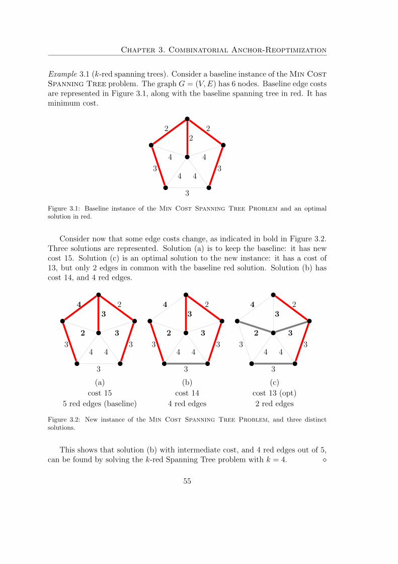
Chapter 3. Combinatorial Anchor-Reoptimization
Example 3.1 (k-red spanning trees). Consider a baseline instance of the Min CostSpanning Tree problem. The graph G = (V,E) has 6 nodes. Baseline edge costsare represented in Figure 3.1, along with the baseline spanning tree in red. It hasminimum cost.
22
4 4
2
3 3
3
4 4
Figure 3.1: Baseline instance of the Min Cost Spanning Tree Problem and an optimalsolution in red.
Consider now that some edge costs change, as indicated in bold in Figure 3.2.Three solutions are represented. Solution (a) is to keep the baseline: it has newcost 15. Solution (c) is an optimal solution to the new instance: it has a cost of13, but only 2 edges in common with the baseline red solution. Solution (b) hascost 14, and 4 red edges.
2
3 3
3
4 4
43
2 3
2
3 3
3
4 4
43
2 3
2
3 3
3
4 4
43
2 3
(a) (b) (c)
cost 15 cost 14 cost 13 (opt)
5 red edges (baseline) 4 red edges 2 red edges
Figure 3.2: New instance of the Min Cost Spanning Tree Problem, and three distinctsolutions.
This shows that solution (b) with intermediate cost, and 4 red edges out of 5,can be found by solving the k-red Spanning Tree problem with k = 4. �
55
Chapter 3. Combinatorial Anchor-Reoptimization
In this chapter, we investigate the complexity of the k-red variant (P-kRed) ofpolynomial combinatorial problems, and especially matroid bases. Let us reviewsome related work. For combinatorial problems, the anchoring level coincideswith transition costs: if element e from the baseline is included in the solution,it yields a profit ae. This model has been studied, e.g., in (Schieber et al., 2018),where the authors considered a special case of the AnchReopt–Cost problem.Spanning trees with a side linear constraint have been widely studied (Aggarwalet al., 1982; Ravi and Goemans, 1996; Ahuja et al., 1993). If the side constraintis any linear constraint, the problem is weakly NP-hard (Aggarwal et al., 1982).In particular, this implies that the Anchor-Reoptimization problem is NP-hardfor non-unit anchoring weights. The biobjective spanning tree has also receivedattention (Hamacher and Ruhe, 1994; Sourd and Spanjaard, 2008).
The chapter is structured as follows. Section 3.1 is devoted to a case study onthe problem of finding a max-weight k-red basis in a matroid. Two approachesare proposed. The first one is an algorithm based on Lagrangian relaxation ofthe k-red constraint, presented in Section 3.1.2. The second one is a polyhedralcharacterization, presented in Section 3.1.3. Both approaches yield a proof that thek-red matroid basis problem is polynomial. In Section 3.2 the result is illustratedfor spanning trees, along with a consequence on the Pareto front of the k-redbiobjective spanning tree. In Section 3.3 the max-weight k-red matching problemin a bipartite graph is considered. We show that a longstanding open problem,Exact Perfect Matching, reduces to this k-red variant.
3.1 Max-weight k-red bases in matroids
Let us study the complexity of finding a max-weight k-red matroid basis. LetM = (E, I) be the matroid and B its set of bases. Let ρ ∈ {0, 1}E be theincidence vector of red elements, and k ∈ N. Let w ∈ RE. Let Bk-red denote theset of bases with at least k-red elements, i.e., Bk-red = {X ∈ B : ρ(X) ≥ k}. Westudy the problem (Bas-kRed) of finding a max-weight solution in Bk-red. It canbe written as the integer program
max wTx
s.t. x ∈ XρTx ≥ k
(Bas-kRed)
Recall that X denote the set of incidence vectors of B, i.e., the feasible set oforiginal problem (P).
In this section, we propose two approaches to solve the (Bas-kRed)problem.Both give a proof of the following result:
56
Chapter 3. Combinatorial Anchor-Reoptimization
Theorem 3.1. The problem (Bas-kRed) of finding a max-weight basis with at leastk red elements is solvable in polynomial time.
The result can be found for spanning trees in (Ahuja et al., 1993; Seref et al.,2009). We here propose a natural extension to matroid bases, and the doublealgorithmic/polyhedral perspective to the problem.
3.1.1 Preliminaries on matroids
Let us give additional definitions and properties on matroids. We refer to Schri-jver’s book (Schrijver, 2003) for details and proofs of the main theorems.
A basis of matroid M is defined as an inclusion-wise maximal independent set.By (ii) in matroid definition (see Page 52), equivalently a basis is an independentset of maximum cardinality. The rank is a function rM : 2E −→ N defined byrM(F ) = max{|I| : I ⊆ F, I ∈ I} for every subset F ⊆ E of elements. Then abasis X has cardinality |X| = rM(E). For X ⊆ E and e ∈ E, let X + e (resp.X − e) denote X ∪ {e} (resp. X \ {e}). Matroids satisfy the following exchangelemma:
Lemma 3.1 (Exchange lemma). Given two bases X and X ′, then for all e ∈X \X ′, there exists f ∈ X ′ \X such that X − e+ f and X ′ − f + e are bases.
Matroids also enjoy nice polyhedral properties. The independent set poly-tope of matroid M is conv{χI : I ∈ I} and the base polytope of matroid M isconv{χB : B ∈ B}. The incidence vector x of an independent set I, and thus anyelement x of the independent set polytope, satisfies inequalities
xe ≥ 0 ∀e ∈ E (3.1)
x(F ) ≤ rM(F ) ∀F ⊆ E (3.2)
Inequality (3.2) is valid since for every I ∈ I and F ⊆ E, it holds that I ∩ F ∈ Ihence |I ∩F | ≤ rM(F ), by definition of the rank. The incidence vector x of a basisB also satisfies
x(E) = rM(E) (3.3)
An important result due to Edmonds is that these inequalities characterize thebase polytope and the independent set polytope.
Theorem 3.2 (Edmonds, see Corollary 40.2b in (Schrijver, 2003)). The polytopes{x ∈ RE : (3.1)–(3.2)} and {x ∈ RE : (3.1)–(3.2)–(3.3)} are integer. They charac-terize the independent set polytope and the base polytope of matroid M , respectively.
57
Chapter 3. Combinatorial Anchor-Reoptimization
Importantly, Theorem 3.2 implies that the Max-Weight Matroid Basisproblem is polynomial, by linear programming. The family of inequalities (2)is exponential, but a polynomial separation algorithm exists (Theorem 40.4 in(Schrijver, 2003)). Hence the maximum of wTx over {x ∈ RE : (3.1)–(3.2)–(3.3)}can be found in polynomial time.
Another result is for the intersection of two matroids.
Theorem 3.3 (Edmonds, see Corollary 41.12a in (Schrijver, 2003)). Let M1 =(E, I1) and M2 = (E, I2) be two matroids on the same ground-set. The polytope ofcommon independent sets conv{χI : I ∈ I1 ∩ I2} is described by inequalities (3.1)and (3.2) associated with both matroids.
Let us finally note that the Min Cost Spanning Tree problem is a specialcase of Max-Weight Basis. With a graph G = (V,E), a matroid MG = (E, IG)is associated where a subset X ⊆ E is an independent set if the set X is cycle-free. Spanning trees are bases of matroid MG. Spanning trees have cardinalityrMG(E) = |V | − 1.
3.1.2 Lagrangian-based algorithm
Let us present the Lagrangian-based approach to (Bas-kRed). In Section 3.1.2.1we present the general framework applicable to any k-red problem (P-kRed). InSection 3.1.2.2 we give further properties specific to k-red matroid bases.
Lagrangian relaxation was used in (Ravi and Goemans, 1996) for the NP-hardconstrained spanning tree and in Example 16.6 in (Ahuja et al., 1993) for a polyno-mial degree-constrained spanning tree problem. The algorithm from Section 3.1.2.2is adapted from this technique, and extended to matroid bases. While preparingthe present work, we found out that in (Seref et al., 2009) the same proof techniquewas used for k-red spanning trees and when red edges form a spanning tree.
3.1.2.1 General approach
Consider Lagrangian relaxation of the k-red constraint ρ(X) ≥ k. Let λ ≥ 0 bethe dual Lagrange multiplier associated with the constraint ρ(X) ≥ k, and letG (λ) be the dual problem
G (λ) : maxX∈X
w(X) + λ(ρ(X)− k)
Let G(λ) be the dual function, i.e., the optimal value of problem G (λ). For a givenλ ≥ 0, the value G(λ) can be computed by solving the problem (P) for modifiedweights we = we+λρe. The k-red problem is maxX∈X minλ≥0w(X)+λ(ρ(X)−k).
58
Chapter 3. Combinatorial Anchor-Reoptimization
Hence it holds that G(λ) is an upper bound to the problem for any value ofmultiplier λ ≥ 0. The best of such upper bounds is the dual bound
minλ≥0G(λ).
In general, the dual bound is not equal to the optimal value of the problem: thereis a Lagrangian duality gap.
A classical optimality condition is as follows. Given λ ≥ 0 and X an optimalsolution of the dual problem G (λ), if λ and X satisfy the complementarity condi-tions ρ(X) ≥ k, (ρ(X) = k or λ = 0), then X is an optimal solution of (P-kRed).Indeed this condition implies w(X) +λ(ρ(X)− k) = w(X), hence the weight of Xis equal to the upper bound G(λ). The solution X being feasible for (P-kRed), itis an optimal solution to (P-kRed).
3.1.2.2 Polynomial algorithm for matroid bases
Let us now give results specific to (Bas-kRed).
Proposition 3.1. For matroid bases, the dual bound minλ≥0 G(λ) is equal to
minλ∈Λ G(λ) where Λ = {wf − we : e, f ∈ E, ρe = 1, ρf = 0}
and thus it can be computed in polynomial time.
Proof. A solution to the dual problem for multiplier λ is a solution to (P) formodified weights w = w + λρ. Recall that an instance of (P) with weights wcan be solved using the greedy algorithm, which compare weights of elements.We assume that if elements have the same weight, the one with smallest indexis picked first. Consider for any instance of (P), the list of elements of E sortedlexicographically by increasing we, then by increasing index. Hence the greedyalgorithm always returns the same solution for all instances whose such list is thesame. Let λ∗ be a value of the multiplier such that the list associated to modifiedweights w changes at λ∗. Then there exists e, f ∈ E such that we ≤ wf if and onlyif λ ≤ λ∗. Hence e is red, f is not red, and λ∗ = wf − we.
The dual function is piecewise affine, and every breakpoint of G(λ) correspondsto a value of the multiplier where the output of the greedy algorithm changes. Bythe previous remark, every breakpoint is in the set Λ = {wf − we : e, f ∈ E, ρe =1, ρf = 0}. This set having quadratic size, the minimum of G(λ) can be foundby evaluating the function at each point of Λ. Note that in case (Bas-kRed) isunfeasible, the minimum of G is unbounded, which can be detected by computingthe value of G in one additional point greater than all points in Λ. Hence the dualbound minλ≥0 G(λ) can be found in polynomial time as claimed.
59
Chapter 3. Combinatorial Anchor-Reoptimization
By Proposition 3.1, the value λ∗ attaining the dual bound G(λ∗) and an optimalsolution X∗ to the dual problem can be found in polynomial time. In generalsolution X∗ does not contain k red edges. In order to show that we can output ak-red solution satisfying the optimality condition, we need the following lemma.
Lemma 3.2. Let w ∈ RE, and W ∗ be the maximum weight of a basis of M .Let k be an integer. Given two bases of weight W ∗ with respectively less and
more than k red elements, there always exists a basis of weight W ∗ with exactly kred elements, and it is computable in polynomial time by Algorithm 1.
Algorithm 1:
Input: X1, X2 ∈ B, k ∈ N such that w(X1) = w(X2) = W ∗ andρ(X1) < k < ρ(X2).
Output: X= ∈ B such that w(X=) = W ∗ and ρ(X=) = k.Let X := X2;while ρ(X) > k do
Let e ∈ X \X1 be a red element;Let f ∈ X1 \X such that X − e+ f ∈ B and X1 − f + e ∈ B;Let X := X − e+ f .
endReturn X;
Proof. Let us prove validity of Algorithm 1. The element e exists because at eachiteration, X has more red elements that X1. The element f exists by the exchangelemma. At each iteration, the set X is a basis. Also, the number of red edgesin X is decremented of at most one at each iteration. Hence when the algorithmterminates, it returns a basis X such that ρ(X) = k.
Let us show that the equality w(X) = W ∗ remains valid at each iteration, i.e.,that w(X − e+ f) = w(X) before the update of X. Since X − e+ f is a basis itcomes w(X − e+ f) ≤ W ∗ = w(X) hence wf ≤ we. Similarly since X1 − f + e isa basis it comes w(X1 − f + e) ≤ W ∗ = w(X1) and we ≤ wf . Thus we = wf andthe weight of X remains equal to W ∗.
Finally it remains to show that this algorithm terminates after a polynomialnumber of iterations. At each update of X, |X1 ∩ X| is incremented. Assumethe algorithm has not terminated after |X \ X1| iterations: then X = X1 henceρ(X) < k, a contradiction. Thus there are at most |X \ X1| iterations and thealgorithm is polynomial.
Let us now present a proof of Theorem 3.1 stated Page 57.
Proof. Let λ0 = 0 < λ1 < . . . < λm be the points of Λ. Let λt∗ ∈ Λ be a point
where G attains its minimum, computed in polynomial time thanks to Proposi-tion 3.1 by exhaustive search on Λ. For every λt ∈ Λ, let X t denote the optimal
60
Chapter 3. Combinatorial Anchor-Reoptimization
solution of (P) computed by the greedy algorithm in interval [λt, λt+1]. In this inter-val the dual function coincides with the linear function λ 7→ w(X t)+λ(ρ(X t)−k).
Let us now exhibit a pair λ, X satisfying the complementarity conditions re-called in Section 3.1.2.1, that is: λ ≥ 0, X is an optimal solution to the dualproblem in λ, and ρ(X) ≥ k, (ρ(X) = k or λ = 0).
(i) Assume first λt∗
= 0. Then G is non-decreasing, and the slope of G on [0, λ1]is non-negative. This slope equals ρ(X0) − k. Hence the pair λ = 0, X0
satisfy the condition and X0 is an optimal solution of (Bas-kRed).(ii) Assume λt
∗> 0. Consider the two solutions X t∗−1 and X t∗ : both are optimal
solutions of the dual problem G (λt∗). Since the dual function attains its
minimum in λt∗
it comes ρ(X t∗−1) − k ≤ 0 and ρ(X t∗) − k ≥ 0. If one ofthem has k red edges, we are done. Otherwise, X t∗−1 and X t∗ satisfy theconditions of Lemma 3.2 for the modified weights associated with λt
∗. Using
Algorithm 1, a solution X= can be computed in polynomial time, such thatX= is also an optimal solution of G (λt
∗), and ρ(X=) = k. Then the condition
is satisfied by λt∗
and X=, hence X= is an optimal solution of (Bas-kRed).
In particular, for (Bas-kRed) problem this implies that there is no Lagrangianduality gap.
3.1.3 Polyhedral characterization
Let us now propose a different approach to solve the (Bas-kRed) problem. LetQ = conv{χB : B ∈ B} denote the base polytope of M . By Edmonds’s resultstated in Theorem 3.2, Q is characterized by inequalities (3.1)–(3.2)–(3.3). LetQk-red = conv{χB : B ∈ Bk-red} be the polytope of problem (Bas-kRed). We areinterested in the characterization of the polytope Qk-red. It holds that Qk-red isincluded in the intersection Q ∩ {x ∈ RE : ρTx ≥ k} of the base polytope withthe k-red half-space. In general, intersecting integer polytope Q with a half-space{x ∈ RE : aTx ≥ k}, a ∈ RE would lead to a set with non-integer extreme points.In general for X ⊆ {0, 1}E and a ∈ RE, the set X ∩ {x ∈ RE : aTx ≥ k} does notadmit an efficient polyhedral characterization. Indeed the problem of maximizingwTx over this set corresponds to AnchReopt–Anch with non-unit anchoringweights, which is NP-hard.
In the case of the k-red constraint, the following polyhedral result holds.
61
Chapter 3. Combinatorial Anchor-Reoptimization
Theorem 3.4. Polytope Qk-red is defined by
xe ≥ 0 ∀e ∈ E (3.1)
x(F ) ≤ rM(F ) ∀F ⊆ E (3.2)
x(E) = rM(E) (3.3)
ρTx ≥ k (3.4)
That is, Qk-red = Q∩ {x ∈ RE : ρTx ≥ k}.
Adding the k-red inequality (3.4) here preserves the integrality of the polytope.
Proof. The proof relies on the identification of the problem (Bas-kRed) as anintersection of matroids. Let m = rM(E). Let ρ denote the incidence vector ofnon-red elements, i.e., ρ = 1 − ρ. Let Mk-red = (E, Ik-red) be a second matroiddefined by: X ∈ Ik-red if ρ(X) ≤ m−k. That is, a subset of elements is independentif it has at most m− k non-red elements. It is a partition matroid.
Then Bk-red = B ∩ Ik-red: indeed a basis X ∈ B has cardinality |X| = m,hence ρ(X) ≤ m − k if and only if ρ(X) ≥ k. Therefore Qk-red = conv{χB : B ∈B ∩ Ik-red}. Using Theorem 3.3, it comes that Qk-red = Q ∩ P , where P is theindependent set polytope of matroid Mk-red.
Let us show that Q∩ {x ∈ RE : ρTx ≥ k} ⊆ Q ∩ P . Let us compute the rankrMk-red(F ) for F ⊆ E. In set F an independent set of max size is formed with: allred elements from F , and a number min(ρ(F ),m− k) of non-red elements. HencerMk-red(F ) = ρ(F ) + min(ρ(F ),m− k).
Let x ∈ Q ∩ {x ∈ RE : ρTx ≥ k}. Let F ⊆ E. Let Fr and Fn denotethe subset of red and non-red elements of F respectively. Then x(F ) = x(Fr) +x(Fn). It holds that x(Fr) ≤ |Fr| = ρ(F ), and similarly x(Fn) ≤ ρ(F ). Moreoverx(Fn) ≤ ρTx = (1 − ρ)Tx ≤ m − k, since x(E) = m and ρTx ≥ k. Thusx(F ) ≤ ρ(F ) + min(ρ(F ),m− k). By Theorem 3.2, P is described by inequalities(1)–(2), here satisfied by x, hence x ∈ P .
Finally this proves Q ∩ {x ∈ RE : ρTx ≥ k} ⊆ Q ∩ P = Qk-red, and Qk-red =Q∩ {x ∈ RE : ρTx ≥ k} as claimed.
The polyhedral result from Theorem 3.4 yields another proof of the polynomial-ity of (Bas-kRed) by linear programming. Indeed solving (Bas-kRed) is equivalentto maximizing wTx over the polytope Qk-red. The inequalities defining Qk-red arein an exponential number, but again the existence of a polynomial separation al-gorithm for inequalities (3.2) ensures that the LP can be solved in polynomialtime.
62
Chapter 3. Combinatorial Anchor-Reoptimization
3.2 Illustration for the k-red spanning tree
Let us now illustrate the results from Section 3.1 for the Min Cost SpanningTree problem. Note first that it is equivalent to look for a min cost or a maxweight spanning tree, since all spanning trees have the same cardinality. For thespanning tree problem, the polyhedral result from Theorem 3.4 can be declined asfollows. Given W ⊆ V , let E[W ] denote the set of edges with both extremities inW . It is known (Edmonds, see Theorem 6.13 in (Korte and Vygen, 2012)) thatthe spanning tree polytope is defined by
xe ≥ 0 ∀e ∈ E (3.1)
x(E[W ]) ≤ |W | − 1 ∀W ⊆ V (3.5)
x(E) = |V | − 1 (3.6)
Corollary 3.1. The polytope of k-red spanning trees is defined by inequalities(3.1)–(3.5)–(3.6) and k-red inequality (3.4).
Let us now consider the k-red spanning tree problem under a bi-objective per-spective. Consider the bi-objective problem of finding x ∈ X with the two objec-tives to maximize: total weight wTx and number of red elements ρTx. A solutionx ∈ X is dominated by solution x′ ∈ X if wTx ≤ wTx′ and ρTx ≤ ρTx′, andone of the inequalities is strict. The Pareto front is formed by all non-dominatedsolutions of X , usually represented in the objective space: that is, a solution x isrepresented by point (ρTx,wTx). For k-red problems, since ρTx takes only integervalues, the Pareto front is formed with a polynomial number of points (k, wTxk),k ∈ {0, . . . , |E|}. Then xk is an optimal solution of the max-weight k-red problem.A solution x∗ is said to be supported if it maximizes a convex combination of theobjectives wTx + λρTx, for some λ ≥ 0. In general for the bi-objective spanningtree, the Pareto front in the objective space is a set with exponential size, and notall non-dominated solutions are supported (Sourd and Spanjaard, 2008). We shownow:
Proposition 3.2. For k-red matroid bases, every point of the Pareto front issupported.
Proof. Consider a point (k,W ) of the Pareto front. The value W is the optimumof the k-red problem. By the previous result from Section 3.1.2, there is no La-grangian duality gap: W equals the dual bound G(λ∗) for some λ∗ ∈ Λ. Followingthe proof of Theorem 3.1, we consider the following cases:
(i) λ∗ = 0. Then the dual problem is simply the original problem with weightsw. An optimal solution to the dual problem is a maximizer of w over X .Thus (k,W ) is supported.
63
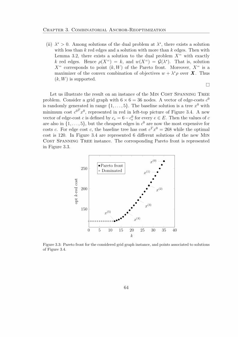
Chapter 3. Combinatorial Anchor-Reoptimization
(ii) λ∗ > 0. Among solutions of the dual problem at λ∗, there exists a solutionwith less than k red edges and a solution with more than k edges. Then withLemma 3.2, there exists a solution to the dual problem X= with exactlyk red edges. Hence ρ(X=) = k, and w(X=) = G(λ∗). That is, solutionX= corresponds to point (k,W ) of the Pareto front. Moreover, X= is amaximizer of the convex combination of objectives w + λ∗ρ over X . Thus(k,W ) is supported.
Let us illustrate the result on an instance of the Min Cost Spanning Treeproblem. Consider a grid graph with 6× 6 = 36 nodes. A vector of edge-costs c0
is randomly generated in range {1, . . . , 5}. The baseline solution is a tree x0 with
minimum cost c0Tx0, represented in red in left-top picture of Figure 3.4. A newvector of edge-cost c is defined by ce = 6− c0
e for every e ∈ E. Then the values of care also in {1, . . . , 5}, but the cheapest edges in c0 are now the most expensive forcosts c. For edge cost c, the baseline tree has cost cTx0 = 268 while the optimalcost is 120. In Figure 3.4 are represented 6 different solutions of the new MinCost Spanning Tree instance. The corresponding Pareto front is representedin Figure 3.3.
0 5 10 15 20 25 30 35 40
150
200
250
x(5)
x(4)
x(3)
x(2)
x(1)
x(0)
k
optk-r
edco
st
Pareto frontDominated
Figure 3.3: Pareto front for the considered grid graph instance, and points associated to solutionsof Figure 3.4.
64
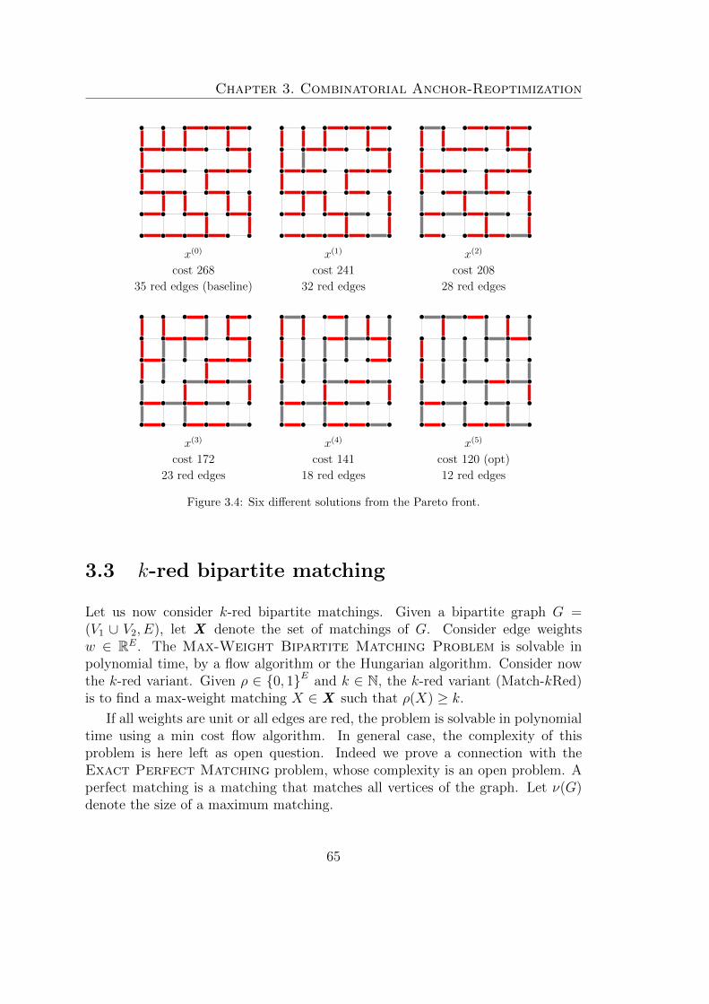
Chapter 3. Combinatorial Anchor-Reoptimization
x(0) x(1) x(2)
cost 268 cost 241 cost 208
35 red edges (baseline) 32 red edges 28 red edges
x(3) x(4) x(5)
cost 172 cost 141 cost 120 (opt)
23 red edges 18 red edges 12 red edges
Figure 3.4: Six different solutions from the Pareto front.
3.3 k-red bipartite matching
Let us now consider k-red bipartite matchings. Given a bipartite graph G =(V1 ∪ V2, E), let X denote the set of matchings of G. Consider edge weightsw ∈ RE. The Max-Weight Bipartite Matching Problem is solvable inpolynomial time, by a flow algorithm or the Hungarian algorithm. Consider nowthe k-red variant. Given ρ ∈ {0, 1}E and k ∈ N, the k-red variant (Match-kRed)is to find a max-weight matching X ∈ X such that ρ(X) ≥ k.
If all weights are unit or all edges are red, the problem is solvable in polynomialtime using a min cost flow algorithm. In general case, the complexity of thisproblem is here left as open question. Indeed we prove a connection with theExact Perfect Matching problem, whose complexity is an open problem. Aperfect matching is a matching that matches all vertices of the graph. Let ν(G)denote the size of a maximum matching.
65
Chapter 3. Combinatorial Anchor-Reoptimization
Exact Perfect Matching
Input: A bipartite graph G = (V1∪V2, E), a subset R ⊆ Eof red edges, an integer k
Question: Is there a perfect matching of the graph with ex-actly k red edges?
Finding a polynomial algorithm to solve the Exact Perfect Matchingis a long-standing open problem since it was introduced in (Papadimitriou andYannakakis, 1982). Non deterministic algorithms are known (Mulmuley et al.,1987), along with algorithms for complete graphs (Yi et al., 2002). Yuster (2012)provides an algorithm that either answers that an exact perfect matching does notexists, or returns a matching with k red edges of size at least ν(G)− 1.
Theorem 3.5. There is a polynomial reduction from Exact Perfect Match-ing to the decision problem associated with (Match-kRed).
Proof. Let G be a bipartite graph with a subset of edges red, k an integer: theyform an instance of the Exact Perfect Matching problem. An instance (G′, ρ, w,W )of the decision version of (Match-kRed) is built as follows: let G′ = G, let ρ bethe indicator of red edges of G, let the weight w be the indicator vector of non-rededges of G, and W = ν(G)− k, where ν(G) is the size of a perfect matching in G.
Assume there exists a perfect matching X of G with exactly k red edges. Thenw(X) = ν(G) − k ≥ W and ρ(X) = k, hence the instance (G′, ρ, w,W ) has a‘yes’ answer. Conversely, let X ′ be a matching of G′ such that ρ(X ′) ≥ k andw(X ′) ≥ ν(G) − k. Hence ρ(X ′) + w(X ′) ≥ ν(G). By definition of ρ and w itholds that ρ(X ′) + w(X ′) = |X ′| ≤ ν(G). Hence X ′ is a perfect matching andequalities ρ(X ′) = k and w(X ′) = ν(G) − k are both satisfied. Therefore thereexists a perfect matching with exactly k red edges in G.
The Lagrangian approach used in the matroid case can also be used for match-ings. It was done, e.g., for the Exact Perfect Matching problem in Yuster(2012), and in Berger et al. (2011) for a budgeted matching problem. However aresult similar to Lemma 3.2, providing an optimal solution from two Lagrangiansolutions, is not to be expected: indeed there may exist a Lagrangian duality gap.
Let us recall a classical result in Lagrangian relaxation, that shows that thetwo approaches for matroid bases are closely related. Consider any k-red prob-lem maxwTx for x ∈ X , ρTx ≥ k. Let Q = convX . For λ ≥ 0, let G(λ) =maxx∈X w
Tx+ λ(ρTx− k).
Proposition 3.3 (Geoffrion, see Theorem 5.36 in (Korte and Vygen, 2012)). Thepolytope Q ∩ {x ∈ RE : ρTx ≥ k} is integer if and only if for any value of theweights w ∈ RE, the dual bound min
λ≥0G(λ) is equal to the optimal value of the
problem.
66
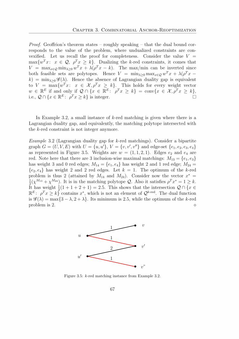
Chapter 3. Combinatorial Anchor-Reoptimization
Proof. Geoffrion’s theorem states – roughly speaking – that the dual bound cor-responds to the value of the problem, where undualized constraints are con-vexified. Let us recall the proof for completeness. Consider the value V =max{wTx : x ∈ Q, ρTx ≥ k}. Dualizing the k-red constraints, it comes thatV = maxx∈Qminλ≥0w
Tx + λ(ρTx − k). The max/min can be inverted sinceboth feasible sets are polytopes. Hence V = minλ≥0 maxx∈Qw
Tx + λ(ρTx −k) = minλ≥0 G (λ). Hence the absence of Lagrangian duality gap is equivalentto V = max{wTx : x ∈ X , ρTx ≥ k}. This holds for every weight vectorw ∈ RE if and only if Q ∩ {x ∈ RE : ρTx ≥ k} = conv{x ∈ X , ρTx ≥ k},i.e., Q∩ {x ∈ RE : ρTx ≥ k} is integer.
In Example 3.2, a small instance of k-red matching is given where there is aLagrangian duality gap, and equivalently, the matching polytope intersected withthe k-red constraint is not integer anymore.
Example 3.2 (Lagrangian duality gap for k-red matchings). Consider a bipartitegraph G = (U, V,E) with U = {u, u′}, V = {v, v′, v′′} and edge-set {e1, e2, e3, e4}as represented in Figure 3.5. Weights are w = (1, 1, 2, 1). Edges e2 and e4 arered. Note here that there are 3 inclusion-wise maximal matchings: M13 = {e1, e3}has weight 3 and 0 red edges; M14 = {e1, e4} has weight 2 and 1 red edge; M24 ={e2, e4} has weight 2 and 2 red edges. Let k = 1. The optimum of the k-redproblem is thus 2 (attained by M14 and M24). Consider now the vector x∗ =12(χM13 + χM24). It is in the matching polytope Q. Also it satisfies ρTx∗ = 1 ≥ k.
It has weight 12(1 + 1 + 2 + 1) = 2.5. This shows that the intersection Q ∩ {x ∈
RE : ρTx ≥ k} contains x∗, which is not an element of Qk-red. The dual functionis G (λ) = max{3− λ, 2 + λ}. Its minimum is 2.5, while the optimum of the k-redproblem is 2. �
u
u′
v
v′
v”
1
1
2
1
Figure 3.5: k-red matching instance from Example 3.2.
67
Chapter 3. Combinatorial Anchor-Reoptimization
Conclusion
We studied k-red variants of polynomial combinatorial problems and especiallymatroid bases. This latter problem is polynomial. While the complexity resultcannot be regarded as a new result, we proposed a complete picture of the problemwith an algorithmic and a polyhedral perspective. In particular, the polyhedralcharacterization will serve on its own for robust approaches.
The approaches are both built upon the properties of matroid bases. Wepointed out that the result cannot be extended in a straightforward manner toother problems, even for bipartite matchings that have a close structure. A per-spective would be to investigate polyhedral characterizations of other k-red prob-lems, first of all, k-red matchings.
68
Chapter 4
Anchor-Robustness forcombinatorial problems
In this chapter we consider a combinatorial problem (P) with ground-set E, definedby min c(X) subject to X ∈ X , where X ⊆ 2E and c(X) =
∑e∈X ce with cost
vector c ∈ RE. Problem (P) is represented by integer program min cTx subject tox ∈ X , with X ⊆ {0, 1}E.
We consider that uncertainty may impair the cost function. Nominal costvector is c ∈ RE. Real cost vector may be cδ = c + δ for δ ∈ ∆, with ∆ theuncertainty set. We assume that costs are non-negative for every uncertaintyrealization, that is, c + δ ≥ 0 for every δ ∈ ∆. By contrast the feasible set X isnot subject to uncertainty.
The concept of anchor-robustness introduced in Chapter 2 is investigated forcombinatorial problems under cost uncertainty. In Section 4.1, the Anchor-Robustproblem (AnchRob) is formally defined, and compared to the recoverable robustproblem (RecovRob) studied in the literature for combinatorial problems. In Sec-tion 4.2 we analyze the complexity of (AnchRob) for discrete and polyhedral un-certainty sets. We point out the connection with other robust approaches. InSection 4.3 we investigate the existence of MIP reformulations for (AnchRob) and(RecovRob). Finally in Section 4.4 we assess the price of anchor-robustness, thatis, the decrease of the optimal value between (AnchRob) and (RecovRob).
4.1 Definitions
Let us first give definitions of anchored solutions and the Anchor-Robust problem.These correspond to the general definitions given in Chapter 2, now specialized tocombinatorial problems.
69
Chapter 4. Combinatorial Anchor-Robustness
4.1.1 Anchored sets
As in Chapter 2, we consider a baseline solution X0 ∈ X , and a collection ofsecond-stage solutions Xδ ∈ X ∀δ ∈ ∆ so that the second-stage solution is chosenafter uncertainty realization δ ∈ ∆ is known. A collection of second-stage collec-tions (Xδ)δ∈∆ can be interpreted as a strategy of a player, who chooses solution Xδ
depending on the adversarial realization of δ ∈ ∆. Given a collection of solutions(Xδ)δ∈∆, the worst-case cost is max
δ∈∆cδ(Xδ). An anchored set is defined as follows.
Definition 4.1 (Anchored set). Let X0 be a baseline solution and (Xδ)δ∈∆ second-stage solutions. A subset H ⊆ E is anchored w.r.t. X0, (Xδ)δ∈∆ if H ⊆ X0 andH ⊆ Xδ for every δ ∈ ∆.
Remark that it is Definition 2.1 from Chapter 2, rewritten in the special caseof binary vectors and equivalence relation =1. An interpretation of Definition 4.1is that elements of H are guaranteed against uncertainty set ∆, since they areselected in the baseline X0 and in every second-stage instance Xδ.
An anchored solution is a triplet (X0, H, (Xδ)δ∈∆) with H ⊆ E a set that isanchored w.r.t. X0, (Xδ)δ∈∆.
Anchored solutions coincide with static-robust solutions when the anchored setis H = X0, as noted in Observation 2.1. Note that since we are considering costuncertainty only, any solution X0 ∈ X is trivially a static-robust solution, i.e., fea-sible for any uncertainty realization. The coincidence with static-robust solutions isuseful for the evaluation of worst-case costs of anchored solutions. With H = X0 isanchored, the worst-case cost of the second-stage instances maxδ∈∆ c
δ(Xδ) is equalto the worst-case cost of the baseline maxδ∈∆ c
δ(X0). Indeed, recall that second-stage costs are non-negative, thus an optimal second-stage solution containing theanchored set H = X0 is just Xδ = X0 for every δ ∈ ∆.
4.1.2 The Anchor-Robust problem
Let us now formulate the Anchor-Robust problem, derived from the general settingpresented in Chapter 2. Consider a 2-stage robust optimization problem where:
– in first stage is decided a baseline solution X0 and an anchored set H ⊆ X0
– in second stage is decided a new solution Xδ such that H ⊆ Xδ
Consider anchoring weights a ∈ RE+. Given k ≥ 0, it will be required that the
anchored set has total anchoring weight at least k. Solutions of the Anchor-Robust problem will be anchored solutions (X0, H, (Xδ)δ∈∆) with anchored set Hsatisfying a(H) ≥ k.
Consider first-stage cost vector C ∈ RE, second-stage cost vector c ∈ RE anduncertainty set ∆. The objective function is the sum of the first-stage cost of the
70
Chapter 4. Combinatorial Anchor-Robustness
baseline and the worst-case cost of second-stage solutions: C(X0)+maxδ∈∆ cδ(Xδ).
This criterion was used in the literature for other robust approaches (see, e.g.,(Hradovich et al., 2017)).
Given feasible set X , costs C, c ∈ RE, uncertainty set ∆, anchoring weightsa ∈ RE
+ and k ≥ 0, the Anchor-Robust (AnchRob) problem is to find an anchoredsolution (X0, (Xδ)δ∈∆, H) such that a(H) ≥ k, and C(X0) + maxδ∈∆ c
δ(Xδ) isminimized. This writes as the following program:
(AnchRob) min C(X0) + max min cδ(Xδ)
X0 ∈ X δ ∈ ∆ Xδ ∈ X
H ⊆ X0 H ⊆ Xδ
a(H) ≥ k
Note that the inner minimization problem is always feasible, since X0 is a feasiblesolution that can be used in second stage. But for a given realization δ ∈ ∆ the costcδ(X0) can be suboptimal, hence a solution Xδ with better cost cδ(Xδ) < cδ(X0)is chosen.
A special case of interest is when anchoring weights are unitary. Then theanchored set must satisfy |H| ≥ k where k is an integer in {0, . . . , |E|}. Anotherspecial case is when C = 0. Then the objective function of (AnchRob) coincidesexactly with the static-robust objective function, that is, the worst-case cost. Notethat for unit anchoring weights and C = 0, the problem is exactly the Worst-caseminimization variant of the anchor-robust problem defined in Chapter 2.
Let us now propose a mathematical program for (AnchRob). Recall that Xdenotes the set of incidence vectors of elements of X . The decision variables areas follows:
– x ∈ X : incidence vector of baseline solution X0;– h ∈ {0, 1}E: incidence vector of the anchored set H;– y ∈ X : incidence vector of the second-stage solution Xδ. Note that y that is
not implicitly indexed with δ, but does depend on the uncertainty realization.
The fact that h represents an anchored set can be enforced by the linear constraints:he ≤ xe for every e ∈ E, and he ≤ ye for every e ∈ E. The (AnchRob) problem isthus:
(AnchRob) min CTx + max min (c+ δ)Ty
x ∈ X δ ∈ ∆ y ∈ Xh ∈ {0, 1}E h ≤ y
h ≤ x
aTh ≥ k
71
Chapter 4. Combinatorial Anchor-Robustness
4.1.3 Connection with the Recoverable-Robust Problem
Let us now present a recoverable robust approach inspired from the literature forthe considered combinatorial problem. Similarly to the (AnchRob) problem, abaseline solution X0 is decided, then a second-stage solution Xδ is decided afterthe uncertainty realization is known. In the recoverable robust approach, thesecond-stage solution must share at least k elements with the first-stage solutions.
We consider the following recoverable-robust problem (RecovRob). The inputsare exactly the same as for (AnchRob), namely, feasible set X , costs C, c ∈ RE,uncertainty set ∆, anchoring weights a ∈ RE
+ and k ≥ 0. The (RecovRob) problemis
(RecovRob) min C(X0) + max min cδ(Xδ)
X0 ∈ X δ ∈ ∆ Xδ ∈ X
a(X0 ∩Xδ) ≥ k
The constraint a(X0 ∩Xδ) ≥ k can be interpreted as a constraint on the distancebetween the baseline solution and the second-stage solution. It can be written asthe existence of a set Hδ, Hδ ⊆ X0, Hδ ⊆ Xδ such that a(Hδ) ≥ k. The differencewith the Anchor-Robust problem is thus the dependency of the set of commondecisions to uncertainty realization δ. In the case of unit anchoring weights, (Re-covRob) is the problem studied in the literature (Kasperski and Zielinski, 2016;Hradovich et al., 2017; Kasperski and Zielinski, 2017).
Using binary vectors x and y to represent sets X0 and Xδ, the constraint|X0 ∩ Xδ| ≥ k (resp. a(X0 ∩ Xδ) ≥ k) can be cast as the quadratic constraintxTy ≥ k (resp.
∑e∈E aexeye ≥ k). The (RecovRob) problem can thus be written
as the following mathematical program:
(RecovRob) min CTx + max min (c+ δ)Ty
x ∈ X δ ∈ ∆ y ∈ X∑e∈E aexeye ≥ k
As a consequence from the connection between (AnchRob) and (RecovRob),the optimal value of (RecovRob) is always better (lower) than the optimal value of(AnchRob). A case where the solutions are not the same, and thus the differencebetween optimal values is strict, was given in Chapter 2.
72
Chapter 4. Combinatorial Anchor-Robustness
4.2 Complexity for discrete and polyhedral
uncertainty sets
In this section, the complexity of (AnchRob) is investigated for a variety of uncer-tainty sets. Note first that (AnchRob) is always harder than the original problem(P). Thus we mostly focus on cases where (P) is solvable in polynomial time, tosee whether there is an increase in complexity in the anchor-robust problem.
We make the even stronger assumption that an efficient polyhedral characteri-zation is known for the original problem. It means that a description of conv(X ) isknown, and either conv(X ) is described by a polynomial number of inequalities orthese inequalities can be separated in polynomial time. Hence the original problem(P) can be solved as the linear program min cTx, x ∈ conv(X ) in polynomial time.This is the case, e.g., for spanning trees, shortest paths, or bipartite matchings.
4.2.1 Uncertainty sets
Let us present the considered uncertainty sets. Let δ ∈ RE+ be a vector, where δe is
the worst-case deviation of the cost of element e. Set ∆ can be a polytope, givenby an outer description
∆ = {(δeue) : u ≥ 0,Mu ≤ β}
where M is a matrix and β a vector with κ lines. In particular we assume (w.l.o.g.
up to a change of δ) that maxu≥0,Mu≤β ue = 1 for every e ∈ E. We assume κpolynomial in |E|, so that optimizing a linear function over ∆ can be done inpolynomial time. Two particular cases are as follows. Given Γ ∈ {0, . . . , |E|}, set∆ is a polyhedral budgeted uncertainty set if
∆ = {(δeue) : ue ∈ [0, 1]E,∑e∈E
ue ≤ Γ}
Set ∆ is a box uncertainty set if
∆ = {(δeue) : ue ∈ [0, 1]E}
which corresponds to the special case where Γ = |E|. Set ∆ can also be definedas a discrete set. In particular, set ∆ is a discrete budgeted set if
∆ = {(δeue) : ue ∈ {0, 1}E,∑e∈E
ue ≤ Γ}
This is budgeted uncertainty as defined in (Bertsimas and Sim, 2004).
73
Chapter 4. Combinatorial Anchor-Robustness
Importantly, note that the uncertainty set cannot be convexified without chang-ing (AnchRob) optimal value. This is to be contrasted with other robust ap-proaches, e.g., static-robustness. For that reason, we consider both polyhedralbudgeted and discrete budgeted sets, though the former is the convex hull of thelatter. Let us illustrate this point on an example.
Example 4.1 (Do not convexify ∆). Consider the Selection problem with n items
and p = 1. Consider nominal costs c = 0. Let δe = 1 for every e ∈ E and Γ = 1.Consider ∆ (resp. conv(∆)) the discrete (resp. polyhedral) budgeted uncertainty
set associated with δ and Γ. Consider the case where there is no first stage, andthe (AnchRob) problem is maxδ∈∆ minx∈X (c + δ)Tx. It can be seen as a gamewhere uncertainty player plays first, then the optimizer player plays second.
– If the uncertainty set is discrete ∆, the uncertainty player adds cost δe = 1to one edge e, then the second player finds a solution with cost 0 by selectingany other element f 6= e.
– If the uncertainty set is polyhedral conv(∆), the uncertainty player can now“split” uncertainty, as δe = 1
nfor every e ∈ E. The second player is then
forced to select a solution with cost 1n.
Optimal values of (AnchRob) for ∆ and conv(∆) are thus different. �
4.2.2 Complexity for extreme values of k
Let us start by analyzing the (AnchRob) problem depending on the value of k,to see when it coincides with other robust problems, and obtain first complexityresults.
4.2.2.1 Case k = 0
Consider first the case where k = 0. No anchored element is required, hencethere is no linking constraint between the baseline solution and the second-stagesolution. The (AnchRob) problem thus boils down to solving independently twoproblems:
– Finding a baseline solution x that minimizes CTx (if there are first-stagecosts). This is simply an instance of the original problem.
– Solving maxδ∈∆ miny∈X (c+ δ)Ty.This latter problem is the adjustable-robust problem (Adj-P), with no first-stagevariable. It is also referred to in the literature as the adversarial problem (see(Nasrabadi and Orlin, 2013; Kasperski and Zielinski, 2016)). It can also be seenas an interdiction problem, where a first player (the uncertainty player) tries toincrease the optimal value of the original problem, by disrupting the elements costs(see (Frederickson and Solis-Oba, 1999)).
Note that in that case k = 0, (AnchRob) and (RecovRob) coincide.
74
Chapter 4. Combinatorial Anchor-Robustness
Proposition 4.1. For k = 0, the (AnchRob) problem is:– polynomial for polyhedral uncertainty;– NP-hard for discrete budgeted uncertainty.
Proof. Consider polyhedral uncertainty. For k = 0, the (AnchRob) problem re-duces to maxδ∈∆ miny∈conv(X )(c+ δ)Ty. Since ∆ and conv(X ) are polytopes, maxand min can be inverted. Replacing maxδ∈∆(c + δ)Ty by its dual, we obtain a
minimization problem min cTy + ηTβ for y ∈ conv(X ), δy ≤ MTη, η ≥ 0, whichis an LP. It is solvable in polynomial time by assumption on conv(X ).
Consider discrete budgeted uncertainty. The NP-hardness result is shown in thespecial case of spanning trees. In (Frederickson and Solis-Oba, 1999) it was shownthat the following problem Spanning Tree Interdiction is NP-complete: givengraph G(V,E), integer Γ ∈ N, edge weight w ∈ {0, 1}E, integer W , decide if thereexists a subset S ⊆ E, |S| ≤ Γ such that the min weight spanning tree in the graph(V,E \S) has weight ≥ W . Let (G = (V,E),Γ, w,W ) be an instance of SpanningTree Interdiction. Let X denote the set of spanning trees of graph G. Letcost vector c = w, δe = (|V | − 1) maxe∈E we, budget Γ. Remark that in the graph
G, for an uncertainty realization δ, edges have either cost we or cost we + δe. Dueto the value of δe, a min spanning tree for costs c+δ uses only edges with cost we ifpossible. The (AnchRob) problem is maxδ∈∆ minx∈X (c+ δ)Tx. Let W ≥ 0. Thenit holds that the optimal value of (AnchRob) is at least W if and only if the answerto the Spanning Tree Interdiction problem on instance (G = (V,E),Γ, w,W )is ‘yes’. Indeed, an uncertainty realization δ ∈ ∆ corresponds to a set S of Γ edgesthat are disrupted to cost δe. There exists a spanning tree in the graph (V,E)with cost W if and only if there exists a spanning tree in the graph (V,E \S) withcost W . The claimed NP-hardness result follows.
4.2.2.2 Case k = kmax
Let us now consider that the original problem satisfies the assumption
All solutions of (P) have the same cardinality kmax. (FixedCard)
This assumption holds for matroid bases.Consider unit anchoring weights and k = kmax. Then the inequality
∑e∈E he ≥
k implies h = x. Given a first-stage solution x, since costs are non-negative asecond-stage optimal solution is y = x. (AnchRob) problem is thus to find astatic-robust solution x minimizing the worst-case cost maxδ∈∆(c+ δ)Tx.
Note that (AnchRob) and (RecovRob) coincide in this case.
Proposition 4.2. Under assumption (FixedCard), (AnchRob) is polynomial fork = kmax for polyhedral budgeted uncertainty and discrete budgeted uncertainty.
75
Chapter 4. Combinatorial Anchor-Robustness
Proof. The complexity of (AnchRob) is the complexity of the static-robust problemfor the considered uncertainty sets. Consider discrete budgeted ∆. Then theproblem is minx∈X maxδ∈∆(c+ δ)Tx. Using the technique from Bertsimas and Sim(Bertsimas and Sim, 2004), it holds that this problem can be solved through |E|+1instances of the original problem (P). Consider now a polyhedral uncertainty set∆. In minx∈X maxδ∈∆(c + δ)Tx the inner max is on a linear function of δ. Henceset ∆ can be convexified without changing the optimal value. The polynomialityresult follows.
4.2.3 Complexity depending on the uncertainty set
Let us now examine how the complexity of (AnchRob) depends on the uncertaintyset: box uncertainty, polyhedral uncertainty, and discrete budgeted uncertainty.
4.2.3.1 Box uncertainty
For box uncertainty, the worst case over ∆ in (AnchRob) is attained for the real-
ization δ = δ: for every y ∈ X , maxδ∈∆(c+ δ)Ty = (c+ δ)Ty. Problem (AnchRob)is then
min CTx+ (c+ δ)Ty
x ∈ Xy ∈ Xh ∈ {0, 1}E
h ≤ x, h ≤ y
aTh ≥ k
It coincides with (RecovRob).
Consider first the case where there are no first-stage costs (C = 0). Thenw.l.o.g. the baseline and the second-stage solution can be set equal. With x = ythe problem corresponds to the AnchReopt–Anch problem with cost functionc + δ. For general C and unit anchoring weights, the problem was specificallystudied for spanning trees (Hradovich et al., 2017) and matroid bases (Lendl et al.,2019) and shown to be solvable in polynomial time. These results are wrapped upin the following proposition:
Proposition 4.3. Under box uncertainty, (AnchRob) for matroid bases is:
– NP-hard for non-unit anchoring weights, even for C = 0;– polynomial for unit anchoring weights.
76
Chapter 4. Combinatorial Anchor-Robustness
4.2.3.2 Polyhedral uncertainty
Let us now consider polyhedral uncertainty, which subsumes box uncertainty.Proposition 4.3 implies that (AnchRob) is NP-hard even for C = 0. Howeverthis relies on non-unit anchoring weights. An open question is the following
Question 4.1. Under polyhedral budgeted uncertainty, what is the complexity of(AnchRob) for matroid bases with unit anchoring weights?
Note that the corresponding question for the (RecovRob) problem, i.e., thecomplexity under polyhedral uncertainty and unit weights, is open even for thespanning tree problem (Kasperski and Zielinski, 2016). It is not clear whetherthe complexity status of (AnchRob) would directly imply the answer to this openquestion. However the same proof technique may be used for both problems.
4.2.3.3 Discrete budgeted uncertainty
In the case of discrete budgeted uncertainty, the result for k = 0 from Proposi-tion 4.1 implies
Proposition 4.4. Under discrete budgeted uncertainty, (AnchRob) is NP-hard.
Note that the result does not rely on anchoring weights.
4.3 MIP reformulations
In this section, we consider polyhedral uncertainty. As shown in Section 4.2, it isa case where the (AnchRob) problem can be NP-hard. To address the problem weinvestigate exact approaches based on mixed-integer programming.
MIP reformulations of static-robust problems (Soyster, 1973; Bertsimas andSim, 2004) were important results advocating for the practical implementabilityof robust optimization. The class of robust 2-stage problems is more challenging.MIP formulations for robust 2-stage problems are often based on an enumeration ofextreme points of the uncertainty set, as noted in the literature review of Chapter 1.By contrast, we investigate MIP formulations where there is no enumeration overthe uncertainty set.
In some special cases, a compact MIP reformulation of (AnchRob) was ob-tained, namely box uncertainty (see Section 4.2.3). The question is to see whethera similar reformulation can be found for more general polyhedral uncertainty sets.We first give a positive result by providing an MIP reformulation for (AnchRob)in Section 4.3.1. Then we discuss the existence of a similar MIP reformulation for(RecovRob) in Section 4.3.2.
77
Chapter 4. Combinatorial Anchor-Robustness
4.3.1 Efficient MIP reformulation for (AnchRob)
Consider polyhedral uncertainty ∆ = {(δeue) : u ≥ 0,Mu ≤ β}. Let η ∈ Rκ+
denote a vector of dual variables associated to the inequalities Mu ≤ β in thedefinition of ∆. Let diag(δ) denote the diagonal matrix of RE×E with (e, e) coeffi-
cient equal to δe. Then for any y ∈ [0, 1]E, the dual of the maximization problem
maxδ∈∆ δTy is to minimize ηTβ for diag(δ)y ≤MTη, η ∈ Rκ
+.For the (AnchRob) problem under polyhedral uncertainty, we obtain the fol-
lowing result
Theorem 4.1. The (AnchRob) problem under polyhedral uncertainty ∆ = {(δeue) :u ≥ 0,Mu ≤ β} and anchoring weights a ∈ RE admits the following MIP refor-mulation (FAnch).
(FAnch) min CTx+ cTy + ηTβ
x ∈ Xy ∈ conv(X )
h ∈ {0, 1}E
h ≤ x
h ≤ y
aTh ≥ k
diag(δ) y ≤MTη
η ∈ Rκ+
Proof. Consider the second-stage minimization problem in (AnchRob): min(c +δ)Ty for y ∈ X , h ≤ y. Note that h ∈ {0, 1}E is fixed. The set Fh = {y ∈[0, 1]E : y ≥ h} is a face of the hypercube [0, 1]E. The second-stage problem isto minimize the linear function (c + δ)Ty for y ∈ X ∩ Fh, or equivalently, fory ∈ conv(X ∩ Fh).
Let us show that conv(X ∩ Fh) = conv(X ) ∩ Fh. Since conv(X ) ⊆ [0, 1]E, theset conv(X ) ∩ Fh is a face of conv(X ). The convex hull conv(X ) is an integerpolytope, hence its restriction to face conv(X ) ∩ Fh is also an integer polytope.
Thus the inner minimization is the linear program min (c + δ)Ty for y ∈conv(X )∩Fh. Because ∆ is a polytope, strong duality gives maxδ∈∆ miny∈conv(X )∩Fh(c + δ)Ty = miny∈conv(X )∩Fh maxδ∈∆(c + δ)Ty. The maximum maxδ∈∆ δ
Ty can be
dualized into ηTβ for diag(δ) y ≤ MTη, η ∈ Rκ+. Plugging into the first-stage
minimization problem of (AnchRob), we obtain the claimed MIP reformulation(FAnch).
Importantly the proof of Theorem 4.1 does not require any further propertyon the set X , except that it is contained in the hypercube.
78
Chapter 4. Combinatorial Anchor-Robustness
The reformulation (FAnch) is an MIP formulation whenever linear inequalitiesdefining X and conv(X ) are known. The size of (FAnch) is polynomial in thesize of the original MIP and the number of constraints κ defining set ∆. Indeedif q denotes the number of constraints defining conv(X ), the MIP reformulation(FAnch) has 3|E| binary variables, |E|+ κ continuous variables, and 2q + 3|E|+ 1linear constraints.
Note that we cannot in general impose y ∈ X . The optimal solution of (FAnch)may have a y-vector that is a fractional point in conv(X ), thus not an extremepoint of conv(X ).
To see this, consider again the instance of Example 4.1. Consider the MIPreformulation (FAnch) in that case. Since k = 0, first-stage solution x can bedropped (set x = y w.l.o.g.). The obtained MIP is to minimize η0 +
∑e∈E ηe for
y ∈ conv(X ) = {y ∈ [0, 1]E :∑
e∈E ye = 1}, ye ≤ η0 + ηe for every e ∈ E, η0 ≥ 0,η ∈ RE
+. An optimal solution of cost 1n
is attained for the fractional point ye = 1n
for every e ∈ E (setting η0 = 1n, ηe = 0 for every e ∈ E). By contrast an integer y
would lead to a solution of cost 1.
In particular, this highlights that a description of conv(X ) is necessary to use(FAnch). For the considered combinatorial problems, a valid formulation is known,i.e., a polytope P such that X = P ∩ {0, 1}E. However replacing conv(X ) by Pin (FAnch) would not lead to a valid reformulation of (AnchRob).
4.3.2 Existence of MIP reformulation for (RecovRob)
Let us now make a connection with (RecovRob), for which an MIP reformulationwould also be of interest. Further assumption on the problem is needed. InChapter 3, we showed that when the original problem (P) is to find a max-weightbasis in a matroid, its feasible set X satisfies the following property: ∀x ∈ X ,conv(X ∩{y :
∑e∈E xeye ≥ k}) = conv(X ) ∩ {y :
∑e∈E xeye ≥ k}. Here x
plays the role of the red edges incidence vector. The equality corresponds to theintegrality of the k-red polytope from Theorem 3.4.
Let us consider problems (P) and anchoring weights a ∈ RE that satisfy asimilar property, denoted by (Integ):
∀x ∈ X , conv
(X ∩ {y :
∑e∈E
aexeye ≥ k}
)= conv(X ) ∩ {y :
∑e∈E
aexeye ≥ k}.
(Integ)Note that the left-hand side set is always included in the right-hand side set. Theassumption (Integ) holds when the polytope conv(X )∩ {y :
∑e∈E aexeye ≥ k} is
integer.
79
Chapter 4. Combinatorial Anchor-Robustness
Let (FRel) denote the relaxation of (FAnch) where h ∈ {0, 1}E is relaxed intoh ∈ [0, 1]E.
Proposition 4.5. If the problem satisfies assumption (Integ), formulation (FRel)is an MIP reformulation for (RecovRob) under polyhedral uncertainty.
Proof. For fixed x ∈ {0, 1}E, let Fx = {y ∈ RE :∑
e∈E aexeye ≥ k}. Con-sider the second-stage minimization problem in (RecovRob): for fixed x ∈ X ,it is to minimize (c + δ)Ty for y ∈ X ∩ Fx. By the assumption (Integ), it ismin (c+ δ)Ty for y ∈ conv(X )∩Fx. Because ∆ is a polytope, strong duality givesmaxδ∈∆ miny∈conv(X )∩Fx(c + δ)Ty = miny∈conv(X )∩Fx maxδ∈∆(c + δ)Ty. The innermaximum can again be dualized. We obtain the (quadratic) reformulation
min CTx+ cTy + ηTβ
x ∈ Xy ∈ conv(X )∑
e∈E aexeye ≥ k
diag(δ) y ≤MTη
η ∈ Rκ+
Now consider linearizing the quadratic constraints. Let h ∈ [0, 1]E. The constraint∑e∈E aexeye ≥ k can be replaced by:
∑e∈E aehe ≥ k, he ≤ xe, he ≤ ye. Then
he ≤ min(xe, ye) which is equal to xeye since xe ∈ {0, 1}. Plugging the linearizationconstraints into the reformulation, we obtain (FRel) as claimed.
Hence (AnchRob) and (RecovRob) have reformulations (FAnch) and (FRel) thatvary only by whether h variables are binary or continuous. However for (Recov-Rob) assumption (Integ) was needed to dualize the recourse problem.
We now show that obtaining a valid reformulation for (RecovRob) as (FRel) ismore an exception, rather than a general rule. Assumption (Integ) was necessaryin the proof of Proposition 4.5; if this assumption is not satisfied, the validity ofthe reformulation may fall down. Let us now formalize this idea. Note first that(FRel) can be written as minx∈X φ(x), where φ(x) is the optimal value of a linearprogram that can be solved in polynomial time. This holds since x ∈ X are theonly binary variables in (FRel).
Proposition 4.6. If P 6= NP, the problem (RecovRob) cannot be reformulated asminx∈X φ(x), where φ(x) is the optimal value of a minimization linear programthat is solvable in polynomial time.
In particular, formulation (FRel) is not always a valid reformulation for (Re-covRob).
80
Chapter 4. Combinatorial Anchor-Robustness
Proof. Let us show that for a given first-stage solution x ∈ X , computing itsoptimal value in a solution of the (RecovRob) can be NP-hard. Consequently ifP 6= NP , (RecovRob) cannot be written as minc∈X φ(x) Consider the followingexample. The underlying problem is matroid basis. The uncertainty set is box,and anchoring weights are a ∈ RE, not unitary. For a given x ∈ X the poly-tope conv(X ) ∩ Fx is not integer, as shown in Chapter 3; thus assumption (Integ)
does not hold. The (RecovRob) is to minimize CTx + (c + δ)Ty for x, y ∈ X ,∑e∈E aexeye ≥ k. This problem is NP-hard for fixed x ∈ X , as noted in Propo-
sition 4.3. By contrast, for fixed x formulation (FRel) is a linear program, thussolvable in polynomial time.
The results from Theorem 4.1 and Proposition 4.6 show that (AnchRob) and(RecovRob) do not have the same properties w.r.t. MIP reformulations. Prob-lem (AnchRob) always has a MIP reformulation, regardless of the problem andanchoring weights. For (RecovRob) the existence of such a reformulation is notalways satisfied. This reveals that (RecovRob) is computationally harder than(AnchRob). It advocates for the use of anchor-robustness, at the expense of solu-tions that have a higher cost w.r.t. recoverable robust solutions. Let us now assessthis increase in cost, referred to as the price of anchor-robustness.
4.4 The price of anchor-robustness
Consider an instance of (AnchRob) (or (RecovRob)) problem, formed with X ,costs c, C, set ∆, unit anchoring weights and integer k. We assume that theproblem (P) satisfies the assumption that all solutions have the cardinality kmax.Let CostAnch(k) and CostRecov(k) denote the optimal values of the (AnchRob) and(RecovRob) respectively. Anchor-robustness and recoverable robustness are botha middle ground between adjustable robustness (case k = 0) and static robustness(case k = kmax). Let CostAdj = CostAnch(0) and CostStat = CostAnch(k
max). Itholds that for every k ∈ {0, . . . , kmax}
CostAdj ≤ CostRecov(k) ≤ CostAnch(k) ≤ CostStat.
We now investigate the gap
PoAR(k) =CostAnch(k)− CostRecov(k)
CostRecov(k)
81
Chapter 4. Combinatorial Anchor-Robustness
that we call the price of anchor-robustness. In the sequel, the price of anchor-robustness is examined both theoretically and numerically.
4.4.1 Unboundedness
A negative result is that
Proposition 4.7. The price of anchor-robustness is unbounded, even for unitanchoring weights and polyhedral budgeted uncertainty.
Proof. Consider the Selection problem, with feasible set X = {x ∈ {0, 1}E :∑e∈E xe = p} for some p ≤ |E|. Consider unit anchoring weights and k = p.
Selection is a special case of matroid bases, hence assumption (Integ) is satisfied.Let C = 0.
Consider problem (AnchRob). Note that the existence of h ∈ {0, 1}E,∑
e∈E he ≥k, y ≥ h implies that h = y, since k = p. Hence y must be an integer solution.Problem (AnchRob) thus writes: miny∈X maxδ∈∆(c + δ)Ty. Hence problem (An-chRob) coincides with the static-robust problem.
Consider now problem (RecovRob). Note that for any y ∈ conv(X ), the equal-ity∑
e∈E ye = p is satisfied. Setting h = y, we get h ∈ [0, 1]E such that∑
e∈E he ≥k. Problem (RecovRob) thus writes: miny∈conv(X ) maxδ∈∆(c+ δ)Ty. Inverting minand max, it is equal to maxδ∈∆ miny∈conv(X )(c + δ)Ty = maxδ∈∆ miny∈X (c + δ)Ty.Hence problem (RecovRob) coincides with the adjustable-robust problem.
Let us now give an example where
CostAdj ≤ CostRecov(k) = 1n< 1 = CostAnch(k) ≤ CostStat.
Let c = 0. Consider polyhedral budgeted uncertainty with Γ = 1 and δe = 1for every e ∈ E. Let p = k = 1. The problem is thus to pick one item. Notethat all items are the same. In problem (AnchRob), one item should be chosen
in first stage. An optimal solution has cost maxδ∈∆ δe = 1 hence CostAnch(k) =1. In problem (RecovRob), an optimal second-stage solution is to pick the iteme ∈ E with minimum deviation δe. Such an item has cost at most 1
n, attained for
uncertainty realization δe = 1n
for every e ∈ E. Hence CostRecov(k) = 1n. Hence
PoAR(k) = n− 1.
4.4.2 Numerical experiments
Let us now evaluate the price of anchor-robustness in numerical experiments, onproblem Selection.
Given integer p, the problem has feasible set X = {x ∈ {0, 1}E :∑
e∈E xe = p}.Its convex hull is conv(X ) = {x ∈ [0, 1]E :
∑e∈E xe = p}. Consider first-stage
82
Chapter 4. Combinatorial Anchor-Robustness
costs C ∈ RE, second-stage costs c ∈ RE, integer k, and polyhedral budgeteduncertainty with budget Γ and deviations δ ∈ RE.
Using Theorem 4.1, a reformulation for the (AnchRob) problem is
min CTx+ cTy + ηΓ +∑
e∈E ρex ∈ {0, 1}E∑
e∈E xe = p
y ∈ [0, 1]E∑e∈E ye = p
h ∈ {0, 1}E
h ≤ x
h ≤ y∑e∈E he ≥ k
δeye ≤ ρe + η ∀e ∈ Eη ≥ 0
ρ ∈ RE+
By Proposition 4.5, a reformulation for (RecovRob) is the MIP where integralityof h is relaxed into h ∈ [0, 1]E.
We consider instances of Selection with E = {1, . . . , n} a set of n = 50items and p = 10. Costs Ce and ce are randomly generated in range {1, . . . , 5} forevery e ∈ E. The uncertainty set is polyhedral budgeted uncertainty set, wheredeviation δe is also randomly generated in range {1, . . . , 5} for every e ∈ E. A
total number of 100 random triplets (C, c, δ) is generated.
The (RecovRob) and (AnchRob) problems can be solved by the MIP refor-mulation derived from Theorem 4.1 which is compact. The corresponding MIPformulations are solved using Julia, JuMP v0.18 and Cplex 12.8. We first mentionthat all instances are solved within a few seconds.
83
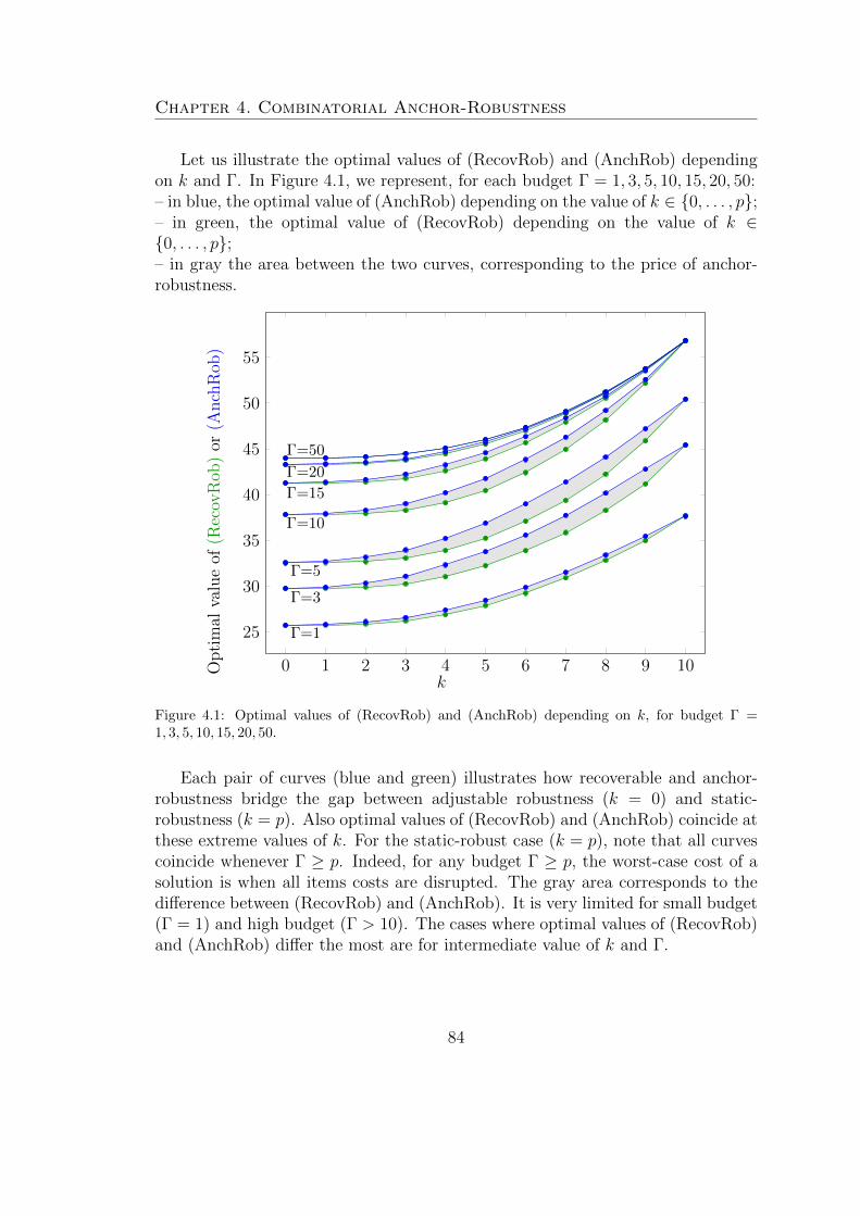
Chapter 4. Combinatorial Anchor-Robustness
Let us illustrate the optimal values of (RecovRob) and (AnchRob) dependingon k and Γ. In Figure 4.1, we represent, for each budget Γ = 1, 3, 5, 10, 15, 20, 50:– in blue, the optimal value of (AnchRob) depending on the value of k ∈ {0, . . . , p};– in green, the optimal value of (RecovRob) depending on the value of k ∈{0, . . . , p};– in gray the area between the two curves, corresponding to the price of anchor-robustness.
0 1 2 3 4 5 6 7 8 9 10
25
30
35
40
45
50
55
Γ=1
Γ=3
Γ=5
Γ=10
Γ=15
Γ=20
Γ=50
k
Opti
mal
valu
eof
(Rec
ovR
ob)
or(A
nch
Rob
)
Figure 4.1: Optimal values of (RecovRob) and (AnchRob) depending on k, for budget Γ =1, 3, 5, 10, 15, 20, 50.
Each pair of curves (blue and green) illustrates how recoverable and anchor-robustness bridge the gap between adjustable robustness (k = 0) and static-robustness (k = p). Also optimal values of (RecovRob) and (AnchRob) coincide atthese extreme values of k. For the static-robust case (k = p), note that all curvescoincide whenever Γ ≥ p. Indeed, for any budget Γ ≥ p, the worst-case cost of asolution is when all items costs are disrupted. The gray area corresponds to thedifference between (RecovRob) and (AnchRob). It is very limited for small budget(Γ = 1) and high budget (Γ > 10). The cases where optimal values of (RecovRob)and (AnchRob) differ the most are for intermediate value of k and Γ.
84
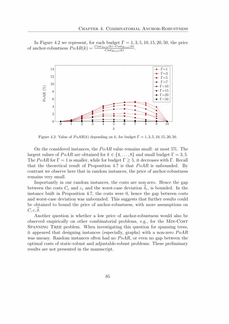
Chapter 4. Combinatorial Anchor-Robustness
In Figure 4.2 we represent, for each budget Γ = 1, 3, 5, 10, 15, 20, 50, the priceof anchor-robustness PoAR(k) = CostAnch(k)−CostRecov(k)
CostRecov(k).
0 1 2 3 4 5 6 7 8 9 100
2
4
6
8
10
12
14
k
PoA
R(%
)
Γ=1Γ=3Γ=5Γ=7Γ=10Γ=15Γ=20Γ=50
Figure 4.2: Value of PoAR(k) depending on k, for budget Γ = 1, 3, 5, 10, 15, 20, 50.
On the considered instances, the PoAR value remains small: at most 5%. Thelargest values of PoAR are obtained for k ∈ {4, . . . , 8} and small budget Γ = 3, 5.The PoAR for Γ = 1 is smaller, while for budget Γ ≥ 5, it decreases with Γ. Recallthat the theoretical result of Proposition 4.7 is that PoAR is unbounded. Bycontrast we observe here that in random instances, the price of anchor-robustnessremains very small.
Importantly in our random instances, the costs are non-zero. Hence the gapbetween the costs Ce and ce and the worst-case deviation δe, is bounded. In theinstance built in Proposition 4.7, the costs were 0, hence the gap between costsand worst-case deviation was unbounded. This suggests that further results couldbe obtained to bound the price of anchor-robustness, with more assumptions onC, c, δ.
Another question is whether a low price of anchor-robustness would also beobserved empirically on other combinatorial problems, e.g., for the Min-CostSpanning Tree problem. When investigating this question for spanning trees,it appeared that designing instances (especially, graphs) with a non-zero PoARwas uneasy. Random instances often had no PoAR, or even no gap between theoptimal costs of static-robust and adjustable-robust problems. These preliminaryresults are not presented in the manuscript.
85
Chapter 4. Combinatorial Anchor-Robustness
Conclusion
In this work we studied the Anchor-Robust approach for combinatorial problemsunder cost uncertainty. The focus was set on original polynomial problems witha polyhedral characterization. We first studied the complexity of the (AnchRob)problem depending on the uncertainty set and the number of anchored decisionsrequired. The problem was shown NP-hard for discrete budgeted uncertainty, andsome cases of polyhedral uncertainty. The hardness results for (AnchRob) are tobe contrasted to existing robust approaches that are tractable for these uncertaintysets. MIP techniques for (AnchRob) were then investigated. An MIP reformula-tion was obtained for (AnchRob), relying on a description of the polytope of theoriginal problem. In parallel, the recoverable robust approach was also examined.It is close to (AnchRob) and similarly provides intermediate solutions betweenadjustable and static-robustness. Most complexity results are common to bothproblems. Concerning MIP reformulations, a strong assumption on the problemis needed to obtain a reformulation for (RecovRob). This reveals the differentnature of problems (AnchRob) and (RecovRob). We then investigated the priceof anchor-robustness. While it is in general unbounded, numerical computationsshowed that it was small in practice on random instances.
There are multiple research perspectives to the work presented in this chapter.The complexity of (AnchRob) could be studied more specifically for some prob-lems. An open question is the complexity of the (AnchRob) problem for spanningtrees, polyhedral budgeted uncertainty and unit anchoring weights. The big pic-ture of the complexity of (AnchRob) on classical polynomial problems is far frombeing complete. On MIP reformulations, it would then be necessary to assess thenumerical performance of the proposed MIP for NP-hard cases of (AnchRob). Aresearch direction is also to extend the MIP tools to new cases, e.g., to design anapproach for (AnchRob) when an efficient description of the problem polytope isnot known. It can be expected that the proposed reformulation could serve as abasis for the design of approximation or decomposition-based exact approaches.Finally, investigation on the price of anchor-robustness could be further carriedout. Better bounds could be searched for, depending on costs and deviationsvalues or properties of the combinatorial problem, and compared to numericalcomputations.
86

Part III
Anchored solutions in projectscheduling
87

Preliminaries on project scheduling
In this part, we study project scheduling problems, a family of problems containingPERT Scheduling.
We consider a project with a set J of n jobs. Let s and t two dummy jobsrepresenting the beginning and the end of the project, and J = J ∪ {s, t}. A jobj ∈ J has processing time pj ≥ 0. A solution of a project scheduling problem isa schedule, i.e., a vector of starting times xi ≥ 0, i ∈ J of the jobs. The startingtime of s is usually xs = 0. The makespan of the schedule is xt.
Various constraints can be imposed on the schedule, leading to distinct projectscheduling problems.
Precedence constraints. Let (J,A) be a precedence graph. It is assumedthat the precedence graph is acyclic, and s (resp. t) is a predecessor (resp. asuccessor) of all jobs. Then precedence constraints are of form
xj − xi ≥ pi ∀(i, j) ∈ A
representing that for every precedence arc (i, j) ∈ A, job j must start after job iis completed. The problem of finding a schedule under precedence constraints, soas to minimize the makespan, is the PERT scheduling problem introduced inPart I.
Generalized precedence constraints. A generalization is to consider con-straints of form
xj − xi ≥ aij ∀(i, j) ∈ Awhere aij is any real number, possibly negative. Such generalized precedenceconstraints can be used to cast time-window constraints, or deadlines. For exemple,if job i should start before date d, this can be represented by the generalizedprecedence constraint xs − xi ≥ −d. Let the precedence graph be (J,A) and let(J,A, a) denote its arc-weighted version. The problem of finding a schedule undergeneralized precedence constraints, so as to minimize the makespan, is the GenPrec Project Scheduling Problem. A schedule satisfying the constraintsof (J,A, a) exists if and only if there exists no positive circuit in (J,A, a). Theminimum makespan is the length of the longest s−t path in (J,A, a), which canbe found in polynomial time by dynamic programming (Pinedo, 2002).
89
Resource constraints. Consider a set of renewable resources R. Assumethat each job i ∈ J has a resource requirement rik of resource k ∈ R duringits execution. The total amount of resource k available is limited, equal to Rk.Resource constraints associated to (r, R) are that at every date d ≥ 0, the totalquantity of resource required by jobs under execution is less than the resourceavailability. This writes∑
i∈J : xi≤d<xi+pi rik ≤ Rk ∀d ≥ 0
Note that schedule x satisfies the resource constraints at all dates if and onlyif it satisfies them at every date xj, j ∈ J where a job starts. The problem offinding a schedule under precedence constraints and resource constraints, so as tominimize the makespan, is the Resource-Constrained Project SchedulingProblem (RCPSP). It has been widely studied in the scheduling literature. Itis NP-hard in the strong sense and computationally challenging (Artigues et al.,2008).
A special case is when there is only one resource type (|R| = 1), every jobhas a resource requirement ri = 1, and the resource availability is an integer m.Then a schedule x satisfies the resource constraints if and only if at every date,there is at most m jobs under execution. This corresponds to executing jobs on midentical machines. In that special case, finding a feasible schedule with minimummakespan is still an NP-hard problem (Garey and Johnson, 1979).
90
Chapter 5
Anchored Rescheduling problemsfor project scheduling
In this chapter we study anchor-reoptimization problems for project scheduling,called anchored rescheduling problems, and analyze their computational complex-ity. The present results have been published in (Bendotti et al., 2020b). Followingthe general definitions of Chapter 2, we study two anchoring levels. The firstone is the number of identical starting times between both schedules. The secondone is the number of starting times that differ from less than a tolerance thresh-old. The anchored rescheduling problem was previously investigated in (Bendottiet al., 2017) for PERT Scheduling with no tolerance, and proved polynomial.We extend the result to GenPrec Project Scheduling, with a tolerance.Generalized precedences allow for a larger variety of constraints such as deadlinesor time windows. The introduction of the tolerance feature also leads to a morerealistic anchored rescheduling problem. We then consider a machine schedulingcase, where the anchored rescheduling problem is shown NP-hard. We define avariant where the sequence of jobs on machines is fixed, resorting to restrictedreoptimization as introduced in Section 2.2.4. It is shown that this simpler, yetpractically attractive, variant is solvable in polynomial time.
5.1 Anchored rescheduling under generalized
precedence
We consider a project scheduling problem Π where a solution is a schedule x ∈ RJ .Given a subset I ⊆ J , a partial assignment of starting times (xi)i∈I is called abaseline. Given an instance I of project scheduling problem Π, a baseline (xi)i∈Iand a solution y of I, the anchoring level is σ(x, y) = |{i ∈ I : xi = yi}|, i.e., the
91
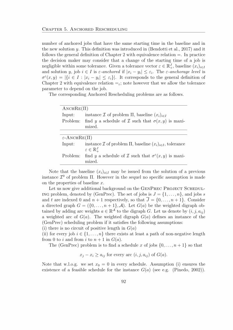
Chapter 5. Anchored Rescheduling
number of anchored jobs that have the same starting time in the baseline and inthe new solution y. This definition was introduced in (Bendotti et al., 2017) and itfollows the general definition of Chapter 2 with equivalence relation =. In practicethe decision maker may consider that a change of the starting time of a job isnegligible within some tolerance. Given a tolerance vector ε ∈ RJ
+, baseline (xi)i∈Iand solution y, job i ∈ I is ε-anchored if |xi − yi| ≤ εi. The ε-anchorage level isσε(x, y) = |{i ∈ I : |xi − yi| ≤ εi}|. It corresponds to the general definition ofChapter 2 with equivalence relation =ε; note however that we allow the toleranceparameter to depend on the job.
The corresponding Anchored Rescheduling problems are as follows.
AnchRe(Π)
Input: instance I of problem Π, baseline (xi)i∈IProblem: find y a schedule of I such that σ(x, y) is maxi-
mized.
ε-AnchRe(Π)
Input: instance I of problem Π, baseline (xi)i∈I , toleranceε ∈ RJ
+
Problem: find y a schedule of I such that σε(x, y) is maxi-mized.
Note that the baseline (xi)i∈I may be issued from the solution of a previousinstance I0 of problem Π. However in the sequel no specific assumption is madeon the properties of baseline x.
Let us now give additional background on the GenPrec Project Schedul-ing problem, denoted by (GenPrec). The set of jobs is J = {1, . . . , n}, and jobs sand t are indexed 0 and n + 1 respectively, so that J = {0, . . . , n + 1}. Considera directed graph G = ({0, . . . , n + 1},A). Let G(a) be the weighted digraph ob-tained by adding arc weights a ∈ RA to the digraph G. Let us denote by (i, j, aij)a weighted arc of G(a). The weighted digraph G(a) defines an instance of the(GenPrec) scheduling problem if it satisfies the following assumptions:(i) there is no circuit of positive length in G(a)(ii) for every job i ∈ {1, . . . , n} there exists at least a path of non-negative lengthfrom 0 to i and from i to n+ 1 in G(a).
The (GenPrec) problem is to find a schedule x of jobs {0, . . . , n+ 1} so that
xj − xi ≥ aij for every arc (i, j, aij) of G(a).
Note that w.l.o.g. we set x0 = 0 in every schedule. Assumption (i) ensures theexistence of a feasible schedule for the instance G(a) (see e.g. (Pinedo, 2002)).
92
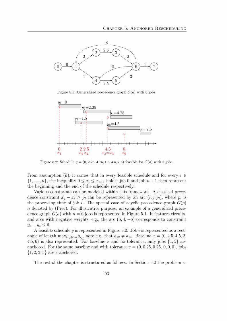
Chapter 5. Anchored Rescheduling
0 1
2 3
4 5
6 70
2
2.5
2
1
1
2.5
3
-8
-6
Figure 5.1: Generalized precedence graph G(a) with 6 jobs.
y1=0
y2=2.25
y3=4.75
y4=1.5
y5=4.5
y6=7.5
0 2.52 4.5 6x1 x2x4 x3=x5 x6
Figure 5.2: Schedule y = (0, 2.25, 4.75, 1.5, 4.5, 7.5) feasible for G(a) with 6 jobs.
From assumption (ii), it comes that in every feasible schedule and for every i ∈{1, . . . , n}, the inequality 0 ≤ xi ≤ xn+1 holds: job 0 and job n+ 1 then representthe beginning and the end of the schedule respectively.
Various constraints can be modeled within this framework. A classical prece-dence constraint xj − xi ≥ pi can be represented by an arc (i, j, pi), where pi isthe processing time of job i. The special case of acyclic precedence graph G(p)is denoted by (Prec). For illustrative purpose, an example of a generalized prece-dence graph G(a) with n = 6 jobs is represented in Figure 5.1. It features circuits,and arcs with negative weights, e.g., the arc (6, 4,−6) corresponds to constrainty6 − y4 ≤ 6.
A feasible schedule y is represented in Figure 5.2. Job i is represented as a rect-angle of length max(i,j)∈A aij, note e.g. that a12 6= a14. Baseline x = (0, 2.5, 4.5, 2,4.5, 6) is also represented. For baseline x and no tolerance, only jobs {1, 5} areanchored. For the same baseline and with tolerance ε = (0, 0.25, 0.25, 0, 0, 0), jobs{1, 2, 3, 5} are ε-anchored.
The rest of the chapter is structured as follows. In Section 5.2 the problem ε-
93
Chapter 5. Anchored Rescheduling
AnchRe(GenPrec) is proven to be solvable in polynomial time. In Section 5.3 wecorrect a flawed complexity result from (Bendotti et al., 2017) in the case of time-window constraints. In Section 5.5 we use our framework in a machine schedulingvariant. In Section 5.4 we analyze the impact of tolerance ε on the optimum ofthe anchored rescheduling problem.
5.2 Polynomiality of ε-AnchRe(GenPrec)
In this section we prove
Theorem 5.1. ε-AnchRe(GenPrec) is solvable in polynomial time.
Let ((xi)i∈I , G(a), ε) be an instance of ε-AnchRe(GenPrec). By testing as-sumptions (i) and (ii), it can be checked in polynomial time that the weighteddigraph G(a) is a valid instance of the (GenPrec) problem.
As done in Chapter 2, we can now define extendable sets, that are subsets ofdecisions that can be maintained in the new solution. Let H ⊆ I be a subset ofjobs. Formally, the set H is x-extendable if there exists a schedule x of G(a) suchthat all jobs in H are ε-anchored with respect to x. Solving ε-AnchRe(GenPrec)is exactly finding a set H x-extendable of maximum size and an associated solutiony.
Consider an auxiliary graph Gaux defined by copying the graph G(a), thenadding for every job i ∈ H two new arcs (0, i, xi − εi) and (i, 0,−(xi + εi)). Theauxiliary graph defines an instance of the (GenPrec) problem, whose constraintsare the constraints from G(a), and the new arcs constraints yi ≥ xi−εi and −yi ≥−(xi+εi), that is exactly |yi−xi| ≤ εi. Hence there is a one-to-one correspondencebetween the schedules of the auxiliary graph Gaux, and the schedules of the instanceG(a) in which all jobs in H are ε-anchored with respect to the baseline x. Thuswe obtain
Proposition 5.1. The set H is x-extendable if and only if the auxiliary graphGaux has no positive circuit.
Let us now show that the absence of positive circuit in Gaux is also equivalentto H ∪ {0} being an antichain in an appropriate poset. Let us denote by `(P )the length of a directed path P in G(a). For every pair of distinct jobs i, j ∈{0, 1, . . . , n}, let LG(a)(i, j) be the maximum length of a directed path from i to jin G(a). By convention it is equal to −∞ if there is no such path. A relation Ron the set of jobs {0, 1, . . . , n} is defined by:
iRj if and only if i = j or xi − εi + LG(a)(i, j) > xj + εj
94
Chapter 5. Anchored Rescheduling
where we define ε0 = 0 for the simplicity of notation. In particular, if i 6= j andiRj, it implies that value LG(a)(i, j) is finite and there exists a path from i to j inG(a).
Lemma 5.1. The relation R is a partial order on the set of jobs {0, 1, . . . , n}.
Proof. Relation R is clearly reflexive. Relation R is antisymmetric: if iRj andjRi with i 6= j, then there exists a longest path Pij from i to j and a longestpath Pji from j to i in G(a). The circuit obtained by closing Pij with Pji haslength LG(a)(i, j) + LG(a)(j, i), which is non-positive by assumption (i) on G(a).Furthermore LG(a)(i, j) + LG(a)(j, i) > xj + εj − (xi − εi) + xi + εi − (xj − εj) =2(εi + εj) ≥ 0, a contradiction. Finally relation R is transitive: consider threepairwise distinct jobs i, j, k such that iRj and jRk. There exists two paths Pijand Pjk in G(a), hence their concatenation (Pij, Pjk) forms a path from i to k. Itcomes xi−εi+LG(a)(i, k) ≥ xi−εi+LG(a)(i, j)+LG(a)(j, k) > xj+εj+LG(a)(j, k) >xk + εk + 2εj ≥ xk + εk. Hence iRk.
Proposition 5.2. The auxiliary graph Gaux has no positive circuit if and only ifH ∪ {0} is an antichain of the poset ({0, 1, . . . , n},R).
Proof. Assume that H ∪ {0} is not an antichain. Then there exists two distinctjobs i and j in H∪{0} such that iRj. Hence there exists a longest path Pij from ito j in G(a). Consider the circuit C obtained by closing the path Pij with the newarc (0, i, xi− εi) if i 6= 0 and with the new arc (j, 0,−(xj + εj)) if j 6= 0. Then thelength of C is LG(a)(i, j) + xi− εi− (xj + εj). Note that it is valid even if i = 0 orj = 0. This length is positive from the definition of R, hence the auxiliary graphcontains a positive circuit.
Conversely, assume that there exists a positive circuit in the auxiliary graph.Then there exists a positive circuit C that contains every vertex at most once.Since G(a) contains no positive circuit, the circuit C contains at least one newarc, and consequently it contains vertex 0 exactly once. It follows that C containsone or two successive new arcs. Let P be the path obtained by removing the newarcs from the circuit C. Let i and j be the first and last vertex of P respectively.The length of C can be written xi − εi + `(P )− (xj + εj) (again it is valid even ifi = 0 or j = 0). By assumption this length is positive, then with `(P ) ≤ LG(a)(i, j)it comes xi − εi + LG(a)(i, j) > xj + εj and iRj.
Remark that all results presented here can be extended to the case of asym-metric tolerance intervals, that is, the case where the starting time of job i isconsidered as unchanged if yi ∈ [xi − ε−i , xi + ε+
i ] with two distinct parametersε−i , ε
+i ≥ 0.
95
Chapter 5. Anchored Rescheduling
We now deduce the proof of the polynomiality result.
Proof of Theorem 5.1. With Proposition 5.1 and Proposition 5.2, a set H is x-extendable if and only if H ∪ {0} is an antichain of the poset ({0, 1, . . . , n},R).Hence solving the reactive problem is tantamount to finding a maximum size an-tichain H ∪{0} of the poset. The latter problem can be solved in polynomial time(Dilworth, 1950). Note also that given a set H∗ of maximum size, a correspondingreactive solution y∗ can be found in polynomial time by computing any scheduleof GH∗ . Hence the problem ε-AnchRe(GenPrec) is polynomial-time solvable.
Algorithmically, a max-size antichain can be found through a combinatorialalgorithm such as Dilworth’s algorithm (Dilworth, 1950), or through linear pro-gramming. A non-compact characterization of the associated polytope is known,together with a polynomial separation algorithm (Schrijver, 2003). Furthermoreanchoring weights may be introduced so that the objective is to maximize thetotal weight of ε-anchored jobs. Then the linear programming approach allowsto search for a max-weight antichain for any weight function, while Dilworth’salgorithm requires integer weights.
Beyond the complexity result, the combination of Proposition 5.1 and Propo-sition 5.2 constitutes a combinatorial characterization of x-extendable sets. Thischaracterization will be of prominent importance in the robust approach devel-opped in Chapter 6. Thus we write it explicitly, in the case ε = 0, in the followingcorollary.
Corollary 5.1 (Characterization of extendable sets). The set H is x-extendableif and only if
xj − xi ≥ LG(a)(i, j) ∀i, j ∈ H ∪ {0}
5.3 Anchored rescheduling with a deadline
constraint
In Chapter 2 we defined two classes of anchor-reoptimization problems, dependingon whether the cost of the new solution is taken into account. For scheduling prob-lems, this amounts to setting an upper bound on the makespan of schedule y, i.e.,to impose a deadline constraint yn+1 ≤ B. The AnchReopt–Cost problem in-troduced in Chapter 2 can then be declined as the following anchored reschedulingproblem
96
Chapter 5. Anchored Rescheduling
ε-AnchRe(Π)-Deadline
Input: instance I of problem Π, baseline (xi)i∈I , toleranceε ∈ RJ
+, deadline B
Problem: find y a schedule of I such that yn+1 ≤ B andσε(x, y) is maximized.
Using generalized precedence constraints, time window constraints of form yi ∈[li, ui] can be modelled with two arcs (0, i, li) and (i, 0,−ui) (recall that y0 = 0w.l.o.g.). In particular, the deadline constraint yn+1 ≤ B can be represented bythe generalized precedence constraint (n+ 1, 0,−B). Consequently
Corollary 5.2. ε-AnchRe(Π)-Deadline is solvable in polynomial time.
We now correct a flawed complexity result from (Bendotti et al., 2017). Inthis previous paper, the so-called Anchor-Reactive CPM-Scheduling Problem withTime Windows (ARSPTW) was defined as a variant of AnchRe(Prec) where thebaseline is a complete schedule (I = J), and a deadline constraint is imposed onthe new schedule: yn+1 ≤ B. Deadline B is part of the instance of the ARSPTW.It follows that the ARSPTW is a special case of ε-AnchRe(Π)-Deadline.
Corollary 5.3. The ARSPTW is polynomial-time solvable.
The proof of Theorem 4.3 from (Bendotti et al., 2017) incorrectly stated theNP-hardness of the ARSPTW. It relied on a reduction from the so-called MaximumComplete Bipartite Subgraph problem (MCBS): given a bipartite graph G = (L∪R,E) with n non isolated nodes and an integer k, is there a complete bipartitesubgraph of G with at least k nodes? The correct reference to Garey and Johnson(1979) requires that the complete bipartite subgraph is balanced, i.e., it has thesame number of nodes in L and R. Without this condition, the MCBS problem ispolynomial-time solvable.
5.4 Sensitivity analysis of ε-AnchRe(GenPrec)
with respect to tolerance
Regarding tolerance ε as a new input of the rescheduling problem, a natural ques-tion is the sensitivity of the optimal value of ε-AnchRe(GenPrec) to ε. In this sec-tion, we study the behavior of the rescheduling optimal value in the case where tol-erance is given by a single parameter ε ≥ 0, that is, εi = ε for every i ∈ {1, . . . , n}.Similar results hold if every εi is any affine function of ε. Given a baseline x andan instance G(a), let
OPT (ε) = maxy schedule
of G(a)
σε(x, y)
97
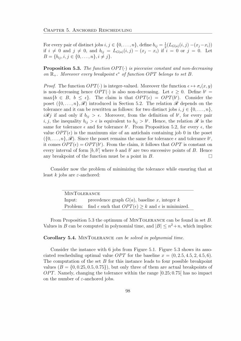
Chapter 5. Anchored Rescheduling
For every pair of distinct jobs i, j ∈ {0, . . . , n}, define bij = 12(LG(a)(i, j) −(xj−xi))
if i 6= 0 and j 6= 0, and bij = LG(a)(i, j) − (xj − xi) if i = 0 or j = 0. LetB = {bij, i, j ∈ {0, . . . , n}, i 6= j}.
Proposition 5.3. The function OPT (·) is piecewise constant and non-decreasingon R+. Moreover every breakpoint ε∗ of function OPT belongs to set B.
Proof. The function OPT (·) is integer-valued. Moreover the function ε 7→ σε(x, y)is non-decreasing hence OPT (·) is also non-decreasing. Let ε ≥ 0. Define bε =max{b ∈ B, b ≤ ε}. The claim is that OPT (ε) = OPT (bε). Consider theposet ({0, . . . , n},R) introduced in Section 5.2. The relation R depends on thetolerance and it can be rewritten as follows: for two distinct jobs i, j ∈ {0, . . . , n},iRj if and only if bij > ε. Moreover, from the definition of bε, for every pairi, j, the inequality bij > ε is equivalent to bij > bε. Hence, the relation R is thesame for tolerance ε and for tolerance bε. From Proposition 5.2, for every ε, thevalue OPT (ε) is the maximum size of an antichain containing job 0 in the poset({0, . . . , n},R). Since the poset remains the same for tolerance ε and tolerance bε,it comes OPT (ε) = OPT (bε). From the claim, it follows that OPT is constant onevery interval of form [b, b′[ where b and b′ are two successive points of B. Henceany breakpoint of the function must be a point in B.
Consider now the problem of minimizing the tolerance while ensuring that atleast k jobs are ε-anchored:
MinTolerance
Input: precedence graph G(a), baseline x, integer k
Problem: find ε such that OPT (ε) ≥ k and ε is minimized.
From Proposition 5.3 the optimum of MinTolerance can be found in set B.Values in B can be computed in polynomial time, and |B| ≤ n2 +n, which implies:
Corollary 5.4. MinTolerance can be solved in polynomial time.
Consider the instance with 6 jobs from Figure 5.1. Figure 5.3 shows its asso-ciated rescheduling optimal value OPT for the baseline x = (0, 2.5, 4.5, 2, 4.5, 6).The computation of the set B for this instance leads to four possible breakpointvalues (B = {0, 0.25, 0.5, 0.75}), but only three of them are actual breakpoints ofOPT . Namely, changing the tolerance within the range [0.25; 0.75[ has no impacton the number of ε-anchored jobs.
98
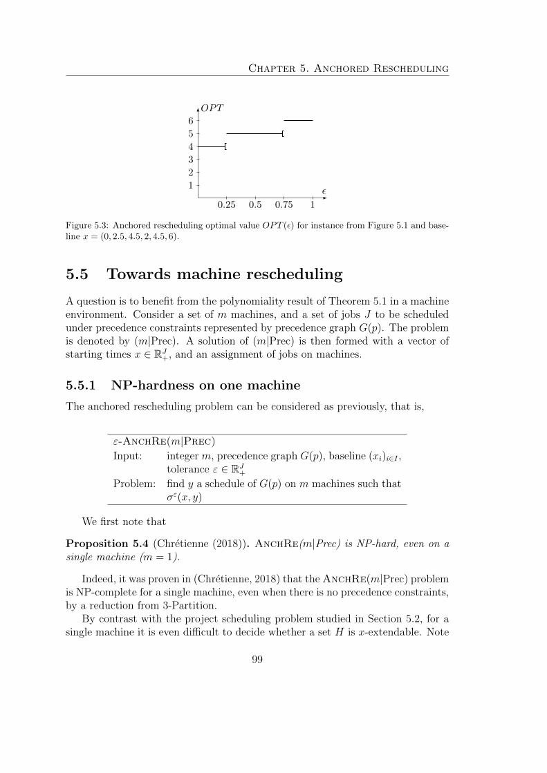
Chapter 5. Anchored Rescheduling
OPT
0.25 0.5 0.75 1
ε1
2
3
4
5
6
Figure 5.3: Anchored rescheduling optimal value OPT (ε) for instance from Figure 5.1 and base-line x = (0, 2.5, 4.5, 2, 4.5, 6).
5.5 Towards machine rescheduling
A question is to benefit from the polynomiality result of Theorem 5.1 in a machineenvironment. Consider a set of m machines, and a set of jobs J to be scheduledunder precedence constraints represented by precedence graph G(p). The problemis denoted by (m|Prec). A solution of (m|Prec) is then formed with a vector ofstarting times x ∈ RJ
+, and an assignment of jobs on machines.
5.5.1 NP-hardness on one machine
The anchored rescheduling problem can be considered as previously, that is,
ε-AnchRe(m|Prec)
Input: integer m, precedence graph G(p), baseline (xi)i∈I ,tolerance ε ∈ RJ
+
Problem: find y a schedule of G(p) on m machines such thatσε(x, y)
We first note that
Proposition 5.4 (Chretienne (2018)). AnchRe(m|Prec) is NP-hard, even on asingle machine (m = 1).
Indeed, it was proven in (Chretienne, 2018) that the AnchRe(m|Prec) problemis NP-complete for a single machine, even when there is no precedence constraints,by a reduction from 3-Partition.
By contrast with the project scheduling problem studied in Section 5.2, for asingle machine it is even difficult to decide whether a set H is x-extendable. Note
99
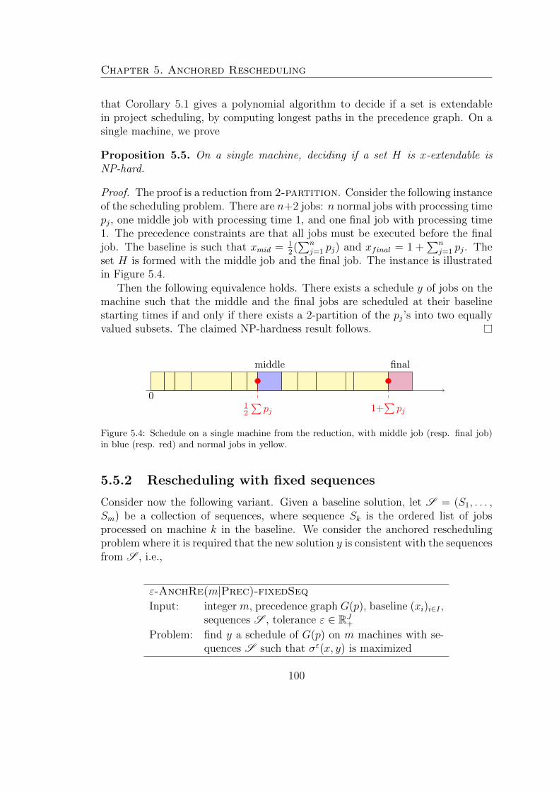
Chapter 5. Anchored Rescheduling
that Corollary 5.1 gives a polynomial algorithm to decide if a set is extendablein project scheduling, by computing longest paths in the precedence graph. On asingle machine, we prove
Proposition 5.5. On a single machine, deciding if a set H is x-extendable isNP-hard.
Proof. The proof is a reduction from 2-partition. Consider the following instanceof the scheduling problem. There are n+2 jobs: n normal jobs with processing timepj, one middle job with processing time 1, and one final job with processing time1. The precedence constraints are that all jobs must be executed before the finaljob. The baseline is such that xmid = 1
2(∑n
j=1 pj) and xfinal = 1 +∑n
j=1 pj. Theset H is formed with the middle job and the final job. The instance is illustratedin Figure 5.4.
Then the following equivalence holds. There exists a schedule y of jobs on themachine such that the middle and the final jobs are scheduled at their baselinestarting times if and only if there exists a 2-partition of the pj’s into two equallyvalued subsets. The claimed NP-hardness result follows.
middle final
12
∑pj 1+
∑pj
0
Figure 5.4: Schedule on a single machine from the reduction, with middle job (resp. final job)in blue (resp. red) and normal jobs in yellow.
5.5.2 Rescheduling with fixed sequences
Consider now the following variant. Given a baseline solution, let S = (S1, . . . ,Sm) be a collection of sequences, where sequence Sk is the ordered list of jobsprocessed on machine k in the baseline. We consider the anchored reschedulingproblem where it is required that the new solution y is consistent with the sequencesfrom S , i.e.,
ε-AnchRe(m|Prec)-fixedSeq
Input: integer m, precedence graph G(p), baseline (xi)i∈I ,sequences S , tolerance ε ∈ RJ
+
Problem: find y a schedule of G(p) on m machines with se-quences S such that σε(x, y) is maximized
100
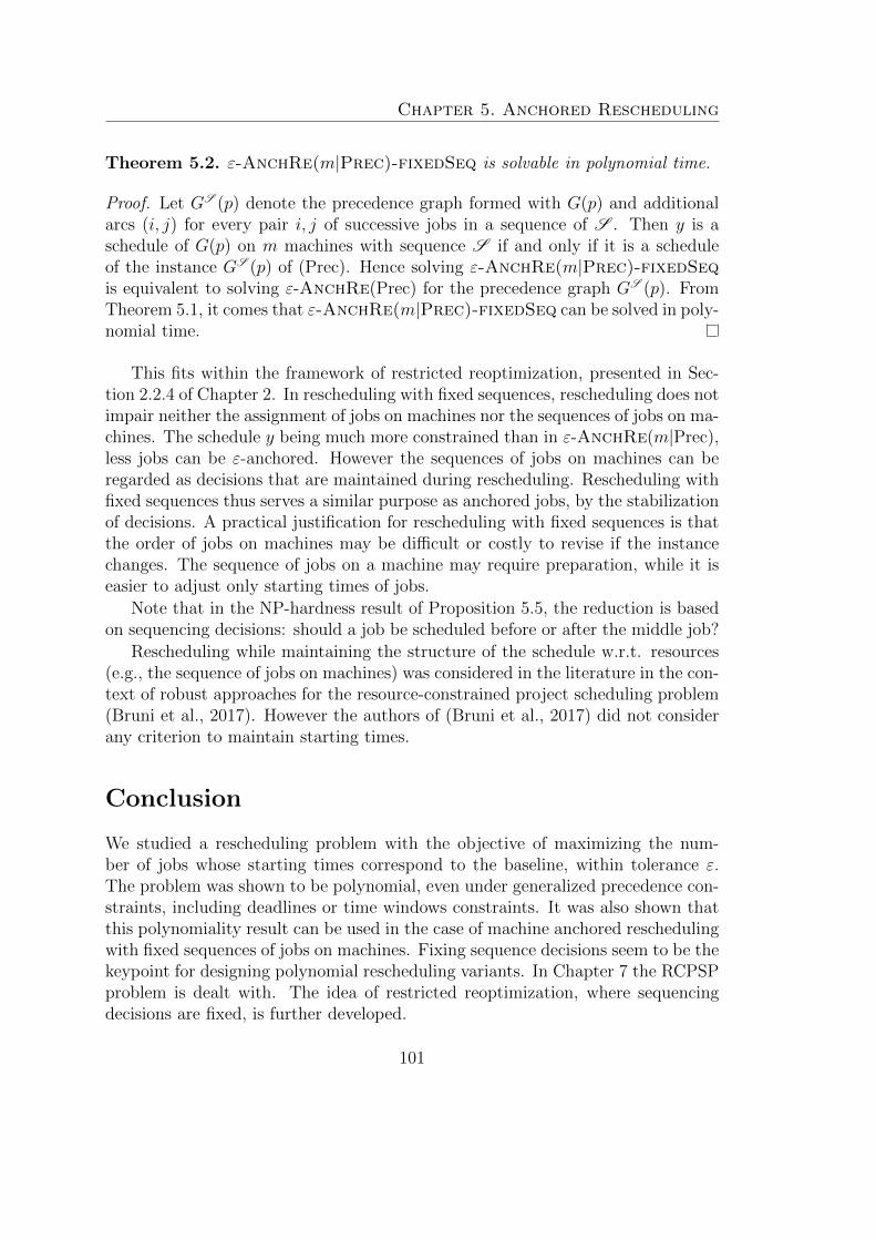
Chapter 5. Anchored Rescheduling
Theorem 5.2. ε-AnchRe(m|Prec)-fixedSeq is solvable in polynomial time.
Proof. Let GS (p) denote the precedence graph formed with G(p) and additionalarcs (i, j) for every pair i, j of successive jobs in a sequence of S . Then y is aschedule of G(p) on m machines with sequence S if and only if it is a scheduleof the instance GS (p) of (Prec). Hence solving ε-AnchRe(m|Prec)-fixedSeqis equivalent to solving ε-AnchRe(Prec) for the precedence graph GS (p). FromTheorem 5.1, it comes that ε-AnchRe(m|Prec)-fixedSeq can be solved in poly-nomial time.
This fits within the framework of restricted reoptimization, presented in Sec-tion 2.2.4 of Chapter 2. In rescheduling with fixed sequences, rescheduling does notimpair neither the assignment of jobs on machines nor the sequences of jobs on ma-chines. The schedule y being much more constrained than in ε-AnchRe(m|Prec),less jobs can be ε-anchored. However the sequences of jobs on machines can beregarded as decisions that are maintained during rescheduling. Rescheduling withfixed sequences thus serves a similar purpose as anchored jobs, by the stabilizationof decisions. A practical justification for rescheduling with fixed sequences is thatthe order of jobs on machines may be difficult or costly to revise if the instancechanges. The sequence of jobs on a machine may require preparation, while it iseasier to adjust only starting times of jobs.
Note that in the NP-hardness result of Proposition 5.5, the reduction is basedon sequencing decisions: should a job be scheduled before or after the middle job?
Rescheduling while maintaining the structure of the schedule w.r.t. resources(e.g., the sequence of jobs on machines) was considered in the literature in the con-text of robust approaches for the resource-constrained project scheduling problem(Bruni et al., 2017). However the authors of (Bruni et al., 2017) did not considerany criterion to maintain starting times.
Conclusion
We studied a rescheduling problem with the objective of maximizing the num-ber of jobs whose starting times correspond to the baseline, within tolerance ε.The problem was shown to be polynomial, even under generalized precedence con-straints, including deadlines or time windows constraints. It was also shown thatthis polynomiality result can be used in the case of machine anchored reschedulingwith fixed sequences of jobs on machines. Fixing sequence decisions seem to be thekeypoint for designing polynomial rescheduling variants. In Chapter 7 the RCPSPproblem is dealt with. The idea of restricted reoptimization, where sequencingdecisions are fixed, is further developed.
101

Chapter 5. Anchored Rescheduling
If the anchored rescheduling problem of an NP-hard problem is bound to remainNP-hard, it is interesting to stress that a polynomial variant can be of practicalinterest. It could be integrated into a robust problem, in order to find a good base-line schedule that could be marginally modified if disruptions occur. A perspectiveis thus to identify such polynomial variants of rescheduling problems, under otherresource constraints.
102
Chapter 6
The Anchor-Robust ProjectScheduling Problem
We consider robust optimization for Project Scheduling under uncertain pro-cessing times. In project management, the decision maker often needs to computea baseline schedule in advance. If processing times are later disrupted, the base-line schedule may become infeasible. Then rescheduling is necessary to recover afeasible solution. The need for stability in rescheduling was pointed out in theliterature review of Chapter 1 and anchor-rescheduling problems were investigatedin Chapter 5. In this chapter we investigate the anchor-robust approach to limitadverse effects of rescheduling by guaranteeing the starting times of some jobs,against realizations of processing times in a given uncertainty set.
For a given uncertainty set, standard robust approaches either produce a sched-ule with a very large makespan, or offer no guarantee on starting times of the jobs.The robust-static approach produces a schedule with very large makespan, thatwould be inapplicable in practice. On the opposite, an adjustable-robust approachis to find the minimum worst-case makespan, at the expense of deciding the sched-ule after the uncertainty realization. Thus there is no baseline solution, and noguarantee on starting times.
In this work, corresponding to (Bendotti et al., 2019), we propose the anchor-robust approach as a middle ground between guaranteeing starting times andguaranteeing the makespan. The output is twofold: a baseline schedule withbounded makespan, and a subset of anchored jobs, that corresponds to guaranteedstarting times in the baseline schedule. Starting times of non-anchored jobs mayneed to be adjusted according to the uncertainty realization to recover a feasibleschedule. Every job is associated with an anchoring weight, representing howbeneficial it is to have a guarantee on the starting time of the job. The Anchor-Robust Project Scheduling Problem (AnchRobPSP) is to find a baseline schedule
103
Chapter 6. Anchor-Robust Project Scheduling
with bounded makespan along with a maximum weight subset of anchored jobs.
The aim of this chapter is to provide an in-depth study of AnchRobPSP, topropose algorithms based on its combinatorial properties. The main contributionsare as follows.
AnchRobPSP is first formulated using graph models. Two graph models areprovided: the first one is applicable to general uncertainty sets, while the secondone is dedicated to budgeted uncertainty sets. These graph models are shown to beconvenient tools to both exhibit hard cases and devise algorithms. In particular,the existence of a compact MIP formulation for AnchRobPSP under budgeteduncertainty is obtained.
Complexity results and algorithms are given for AnchRobPSP under the fol-lowing uncertainty sets. For box uncertainty sets, we show that AnchRobPSP issolvable in polynomial time. For upper-bounded uncertainty sets, we show thatAnchRobPSP is co-NP-hard. For budgeted uncertainty sets, we first show thatthe decision version of AnchRobPSP is NP-complete, even in restricted cases withfixed budget. (Pseudo-)polynomial algorithms are then given for special cases,depending on the uncertainty set and the precedence graph.
A computational evaluation highlights the characteristics of optimal solutionsof AnchRobPSP and the impact of parameters. The proposed approaches to solveAnchRobPSP are shown to be competitive with classical affine decision rules fromthe literature.
6.1 The Anchor-Robust Project Scheduling
Problem
In this section we first define formally the AnchRobPSP problem, the considereduncertainty sets, and point out connections with classical robust approaches.
6.1.1 Problem definition
Let us recall some notation for the original Project Scheduling problem. A setof jobs J = {1, . . . , n} must be scheduled while respecting precedence constraints,represented by a directed acyclic graph G = (J,A). The vertex-set of G is J =J∪{s, t} where s (resp. t) is a predecessor (resp. successor) of all jobs, representingthe beginning (resp. the end) of the schedule. Each job i ∈ J has a processingtime pi ∈ R+, and ps = 0. Given a vector p ∈ RJ
+, let G(p) be the weighteddigraph obtained from G by weighting every arc (i, j) with pi. A schedule of G(p)
104
Chapter 6. Anchor-Robust Project Scheduling
is a vector of starting times x ∈ RJ+ such that xj − xi ≥ pi for every arc (i, j) of
G(p), xs = 0. Then xt is the makespan of the schedule.
We consider a 2-stage decision process to deal with uncertain processing timesof jobs. At first stage, the decision maker has a baseline instance G(p) to solve,and a deadline M ≥ 0. He must choose a baseline schedule, i.e., a schedule of G(p)with makespan at most M . At second stage, the decision maker will know the realinstance G(p + δ) where δ ∈ RJ
+ is the vector of disruptions on processing times.Then a second-stage schedule xδ of G(p+ δ) will be determined. We consider thatthe decision maker wants to hedge against a family {G(p + δ)}δ∈∆ of instances,where the set ∆ is the uncertainty set. In order to have guarantees on startingtimes, we are interested in jobs for which the starting time in the baseline schedulex0 will be the same as the starting time in any second-stage schedule xδ. Formally
Definition 6.1. Given a baseline schedule x0, a subset H of jobs is anchored withrespect to x0 if for every δ ∈ ∆, there exists a schedule xδ of G(p + δ) such thatx0i = xδi for every i ∈ H.
Note that it corresponds to Definition 2.1 from Chapter 2 in the case of con-tinuous variables with equivalence relation =.
Each job i ∈ J is associated with an anchoring weight ai ∈ R+. Given abaseline instance G(p), an uncertainty set ∆, anchoring weights a ∈ RJ
+, and adeadline M , the Anchor-Robust Project Scheduling Problem (AnchRobPSP) is tofind a baseline schedule x0 and a subset H ⊆ J anchored with respect to x0, sothat the total weight a(H) =
∑i∈H ai is maximized.
(AnchRobPSP) is a robust 2-stage problem that can be written as the followingprogram:
(AnchRobPSP): max min max a(H)
x0 schedule of G(p) δ ∈ ∆ xδ schedule of G(p+ δ)
x0t ≤M xδj = x0
j ∀j ∈ HH ⊆ J
Uncertainty appears in the right-hand side of precedence constraints. Also,since H is decided in first stage, the recourse problem is a linear program withconstant objective function, i.e., it is a feasibility problem. Set H is an anchoredset if and only if the inner min/max has value a(H); otherwise it has value −∞.It corresponds to the Anchored set maximization variant of the Anchor-Robustproblem, proposed in generic form in Chapter 2.
105
Chapter 6. Anchor-Robust Project Scheduling
A previous reference is the proactive problem denoted by DAPSP in (Bendottiet al., 2017). It is also a robust 2-stage problem that can be written similarly asa max/min/max program, but with the set H being a recourse variable. In otherwords the set H would appear in the inner maximization problem for DAPSP,rather than in the outer maximization problem for AnchRobPSP. The complexityof DAPSP was studied in (Bendotti et al., 2017) for the special case of box uncer-tainty. From a practical point of view, AnchRobPSP offers a stronger guaranteeon starting times, since the anchored jobs are known in first stage. We refer toSection 2.3.4 for a generic comparison between the two problems.
6.1.2 Uncertainty sets
Let us now give definitions of the considered uncertainty sets. Let ∆ ⊆ RJ+.
The set ∆ is referred to as a general uncertainty set when no further condition isimposed. The set ∆ is an upper-bounded uncertainty set if there exists δ+ ∈ RJ
+
such that for every δ ∈ ∆, δ+i ≥ δi for every i ∈ J , i.e., the duration of job i
in a second-stage instance is at most pi + δ+i . Note that δ+ is not necessarily
an element of ∆ because it is unlikely that all jobs have maximum duration atthe same time. The set ∆ is a box uncertainty set if ∆ = Πi∈J [δ−i , δ
+i ] for some
δ−, δ+ ∈ RJ+. The set ∆ is a budgeted uncertainty set associated with vector
δ ∈ RJ+ and integer Γ ∈ {1, . . . , n} if ∆ =
{(δiui)i∈J : ui ∈ {0, 1}J ,
∑i∈J ui ≤ Γ
}.
Budget Γ corresponds to the maximum number of disruptions that can occur atthe same time (Bertsimas and Sim, 2004).
Note that the uncertainty set ∆ can be convexified without changing feasi-ble solutions. This result is well-known for robust 2-stage linear programs, seee.g., Theorem 2.2 in (Ben-Tal et al., 2004). It can be checked that it appliessimilarly to AnchRobPSP. It stems from the fact that combinatorial decisions(for deciding set H) are taken in first stage. Consequently, it is equivalent to
consider the budgeted uncertainty set defined by Γ and δ, or its convex hull{(δiui)i∈J : ui ∈ [0, 1]J ,
∑i∈J ui ≤ Γ
}. In this latter case, more than Γ jobs may
have a non-zero disruption δi.
Let us illustrate AnchRobPSP on a simple example for these uncertainty sets.Consider a project scheduling instance with 5 jobs. The precedence graph is rep-resented in Figure 6.1. Nominal processing times are p = (1, 1, 1, 1, 2). Each job is
also associated with a worst-case deviation δ = (0.5, 1, 0.5, 0.5, 0.5). In Figure 6.1,
each arc (i, j) is weighted with value pi + δi. Let the deadline be M = 4.5.
106
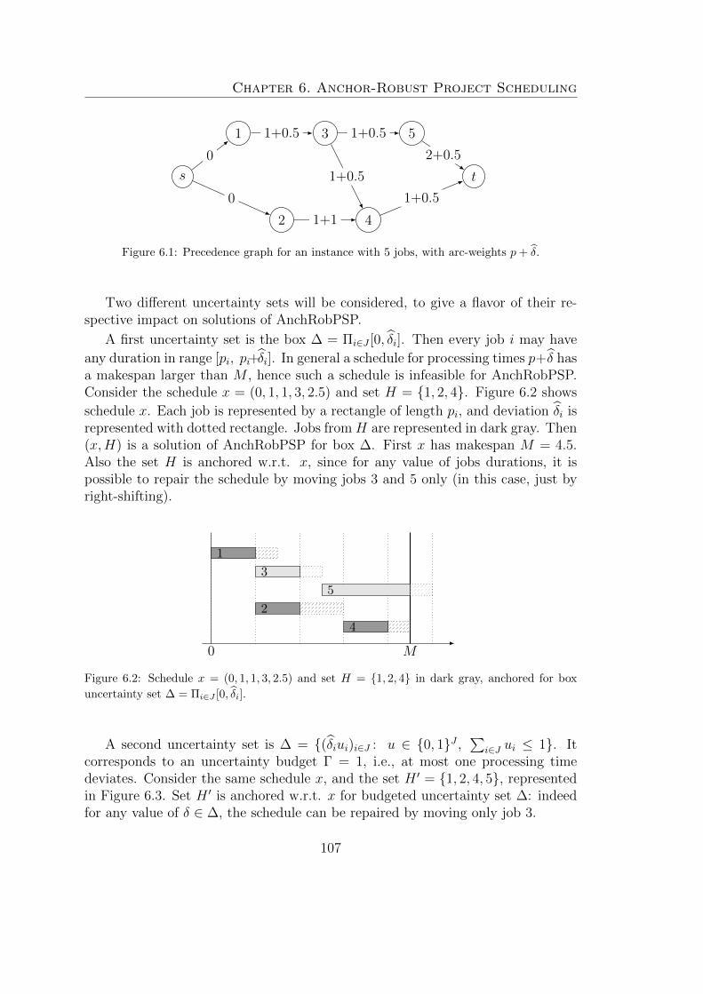
Chapter 6. Anchor-Robust Project Scheduling
s
1
2
3
4
5
t
0
0
1+0.5 1+0.5
1+1
1+0.5
2+0.5
1+0.5
Figure 6.1: Precedence graph for an instance with 5 jobs, with arc-weights p+ δ.
Two different uncertainty sets will be considered, to give a flavor of their re-spective impact on solutions of AnchRobPSP.
A first uncertainty set is the box ∆ = Πi∈J [0, δi]. Then every job i may have
any duration in range [pi, pi+δi]. In general a schedule for processing times p+δ hasa makespan larger than M , hence such a schedule is infeasible for AnchRobPSP.Consider the schedule x = (0, 1, 1, 3, 2.5) and set H = {1, 2, 4}. Figure 6.2 shows
schedule x. Each job is represented by a rectangle of length pi, and deviation δi isrepresented with dotted rectangle. Jobs from H are represented in dark gray. Then(x,H) is a solution of AnchRobPSP for box ∆. First x has makespan M = 4.5.Also the set H is anchored w.r.t. x, since for any value of jobs durations, it ispossible to repair the schedule by moving jobs 3 and 5 only (in this case, just byright-shifting).
0 M
1
3
5
2
4
Figure 6.2: Schedule x = (0, 1, 1, 3, 2.5) and set H = {1, 2, 4} in dark gray, anchored for box
uncertainty set ∆ = Πi∈J [0, δi].
A second uncertainty set is ∆ = {(δiui)i∈J : u ∈ {0, 1}J ,∑
i∈J ui ≤ 1}. Itcorresponds to an uncertainty budget Γ = 1, i.e., at most one processing timedeviates. Consider the same schedule x, and the set H ′ = {1, 2, 4, 5}, representedin Figure 6.3. Set H ′ is anchored w.r.t. x for budgeted uncertainty set ∆: indeedfor any value of δ ∈ ∆, the schedule can be repaired by moving only job 3.
107
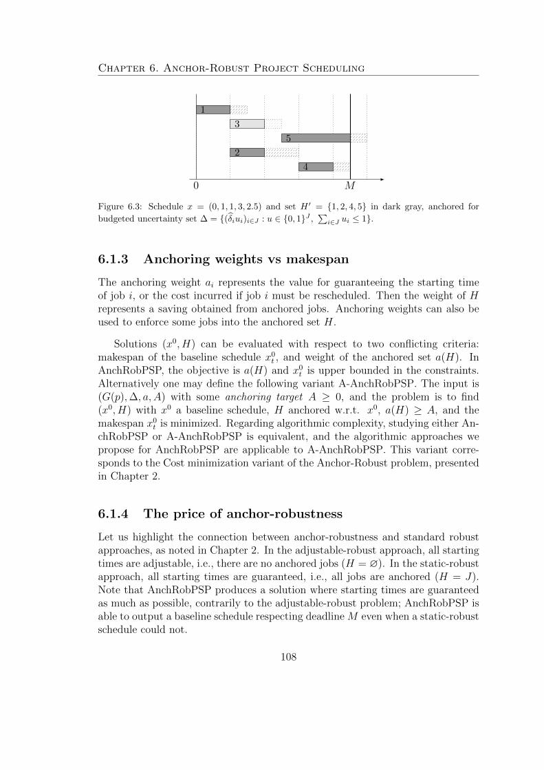
Chapter 6. Anchor-Robust Project Scheduling
0 M
1
3
5
2
4
Figure 6.3: Schedule x = (0, 1, 1, 3, 2.5) and set H ′ = {1, 2, 4, 5} in dark gray, anchored for
budgeted uncertainty set ∆ = {(δiui)i∈J : u ∈ {0, 1}J ,∑i∈J ui ≤ 1}.
6.1.3 Anchoring weights vs makespan
The anchoring weight ai represents the value for guaranteeing the starting timeof job i, or the cost incurred if job i must be rescheduled. Then the weight of Hrepresents a saving obtained from anchored jobs. Anchoring weights can also beused to enforce some jobs into the anchored set H.
Solutions (x0, H) can be evaluated with respect to two conflicting criteria:makespan of the baseline schedule x0
t , and weight of the anchored set a(H). InAnchRobPSP, the objective is a(H) and x0
t is upper bounded in the constraints.Alternatively one may define the following variant A-AnchRobPSP. The input is(G(p),∆, a, A) with some anchoring target A ≥ 0, and the problem is to find(x0, H) with x0 a baseline schedule, H anchored w.r.t. x0, a(H) ≥ A, and themakespan x0
t is minimized. Regarding algorithmic complexity, studying either An-chRobPSP or A-AnchRobPSP is equivalent, and the algorithmic approaches wepropose for AnchRobPSP are applicable to A-AnchRobPSP. This variant corre-sponds to the Cost minimization variant of the Anchor-Robust problem, presentedin Chapter 2.
6.1.4 The price of anchor-robustness
Let us highlight the connection between anchor-robustness and standard robustapproaches, as noted in Chapter 2. In the adjustable-robust approach, all startingtimes are adjustable, i.e., there are no anchored jobs (H = ∅). In the static-robustapproach, all starting times are guaranteed, i.e., all jobs are anchored (H = J).Note that AnchRobPSP produces a solution where starting times are guaranteedas much as possible, contrarily to the adjustable-robust problem; AnchRobPSP isable to output a baseline schedule respecting deadline M even when a static-robustschedule could not.
108
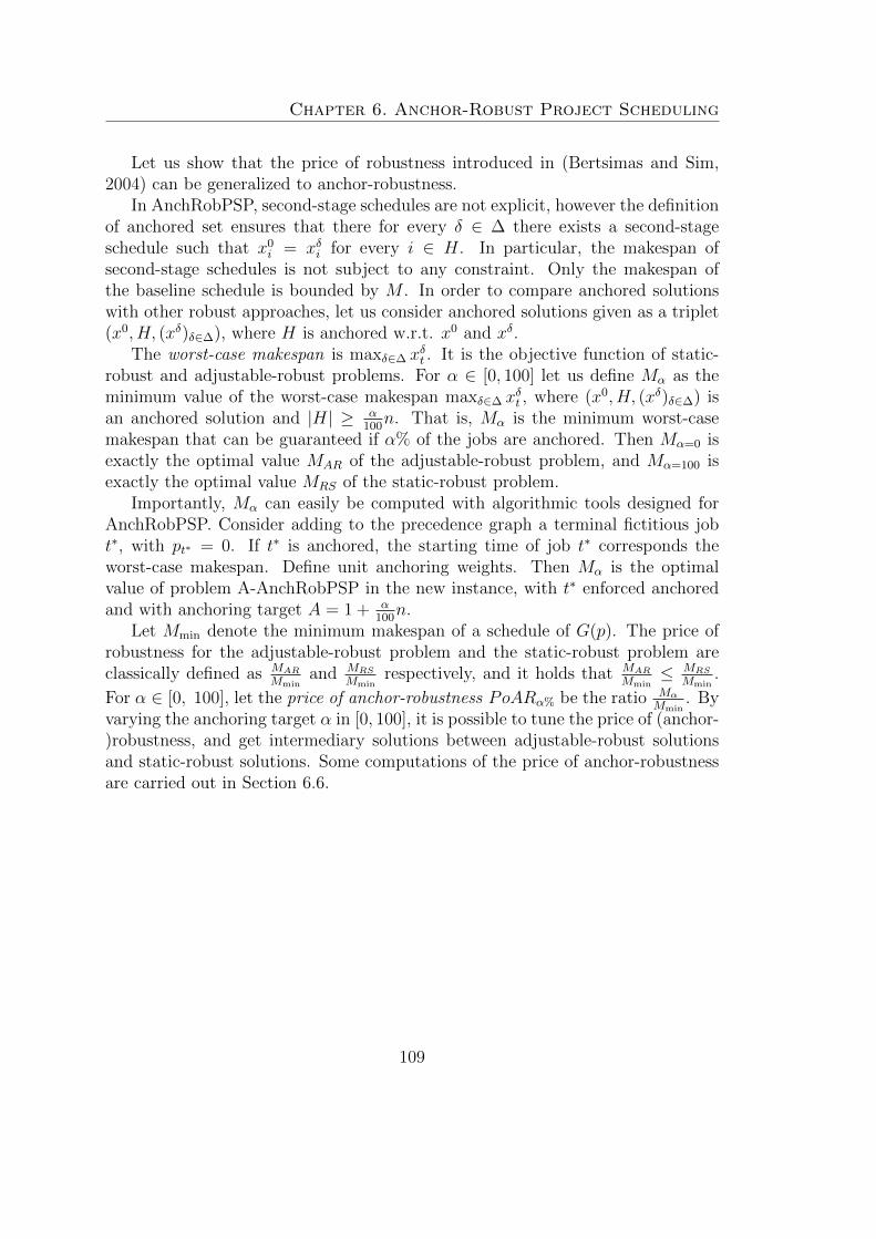
Chapter 6. Anchor-Robust Project Scheduling
Let us show that the price of robustness introduced in (Bertsimas and Sim,2004) can be generalized to anchor-robustness.
In AnchRobPSP, second-stage schedules are not explicit, however the definitionof anchored set ensures that there for every δ ∈ ∆ there exists a second-stageschedule such that x0
i = xδi for every i ∈ H. In particular, the makespan ofsecond-stage schedules is not subject to any constraint. Only the makespan ofthe baseline schedule is bounded by M . In order to compare anchored solutionswith other robust approaches, let us consider anchored solutions given as a triplet(x0, H, (xδ)δ∈∆), where H is anchored w.r.t. x0 and xδ.
The worst-case makespan is maxδ∈∆ xδt . It is the objective function of static-
robust and adjustable-robust problems. For α ∈ [0, 100] let us define Mα as theminimum value of the worst-case makespan maxδ∈∆ x
δt , where (x0, H, (xδ)δ∈∆) is
an anchored solution and |H| ≥ α100n. That is, Mα is the minimum worst-case
makespan that can be guaranteed if α% of the jobs are anchored. Then Mα=0 isexactly the optimal value MAR of the adjustable-robust problem, and Mα=100 isexactly the optimal value MRS of the static-robust problem.
Importantly, Mα can easily be computed with algorithmic tools designed forAnchRobPSP. Consider adding to the precedence graph a terminal fictitious jobt∗, with pt∗ = 0. If t∗ is anchored, the starting time of job t∗ corresponds theworst-case makespan. Define unit anchoring weights. Then Mα is the optimalvalue of problem A-AnchRobPSP in the new instance, with t∗ enforced anchoredand with anchoring target A = 1 + α
100n.
Let Mmin denote the minimum makespan of a schedule of G(p). The price ofrobustness for the adjustable-robust problem and the static-robust problem areclassically defined as MAR
Mminand MRS
Mminrespectively, and it holds that MAR
Mmin≤ MRS
Mmin.
For α ∈ [0, 100], let the price of anchor-robustness PoARα% be the ratio Mα
Mmin. By
varying the anchoring target α in [0, 100], it is possible to tune the price of (anchor-)robustness, and get intermediary solutions between adjustable-robust solutionsand static-robust solutions. Some computations of the price of anchor-robustnessare carried out in Section 6.6.
109
Chapter 6. Anchor-Robust Project Scheduling
6.2 Graph Models for the Anchor-Robust
Project Scheduling Problem
Let us first restate a technical result that will be used in the sequel. Let G be adirected acyclic graph with vertex-set J = J ∪{s, t} and let G(π) be the weighted
digraph obtained by adding arc-weight πij ∈ R+ to every arc (i, j) of G. Note that
G(π) is a precedence graph for project scheduling under generalized precedence.
Given a path P in G(π), the length of the path P in G(π) is denoted by `G(π)(P ).
Given two vertices i, j ∈ J , let LG(π)(i, j) be the length of the longest i−j path in
G(π) (or −∞ if there is no i−j path in G(π)). Given x ∈ RJ+ and H ⊆ J , let xH
denote the restriction of vector x to H, i.e., xH = (xi)i∈H .
In Chapter 5 we gave a characterization of extendable sets, i.e., subsets ofstarting times from a baseline that can be extended into a new solution of aproject scheduling instance. Let us restate this result as a lemma.
Lemma 6.1. Given G(π), a set H ⊆ J and x0H a vector of RH
+ , there exists a
schedule x of G(π) such that xH = x0H if and only if x0
j −x0i ≥ LG(π)(i, j) for every
i, j ∈ H ∪ {s}.
Let (G(p),∆,M, a) be an instance of AnchRobPSP. It is assumed throughoutthe paper that LG(p)(s, t) ≤M , namely, a baseline schedule always exists.
6.2.1 A General-Purpose Graph Model
Let ∆ be a general uncertainty set. For every i, j ∈ J , let L∆ij = max
δ∈∆LG(p+δ)(i, j).
Let G∆ be the weighted digraph obtained by taking the transitive closure of theprecedence graph G, and adding the arc-weight L∆
ij on each arc (i, j) with j 6= t,and the arc-weight LG(p)(i, t) on each arc (i, t). Given H ⊆ J , let G∆[H] denotethe subgraph of G∆ induced by H ∪ {s, t}. An example of an instance with 5jobs and processing times p = (2, 1, 2, 1, 2) is represented in Figure 6.4(a) with aprecedence graph G(p) and in Figure 6.4(b) with the associated graph G∆ for thebox uncertainty set ∆ = Πi∈J [0, δ+
i ] with δ+ = (2, 1, 2, 1, 1). Note that in this caseL∆ij = LG(p+δ+)(i, j) for every i, j ∈ J .
110
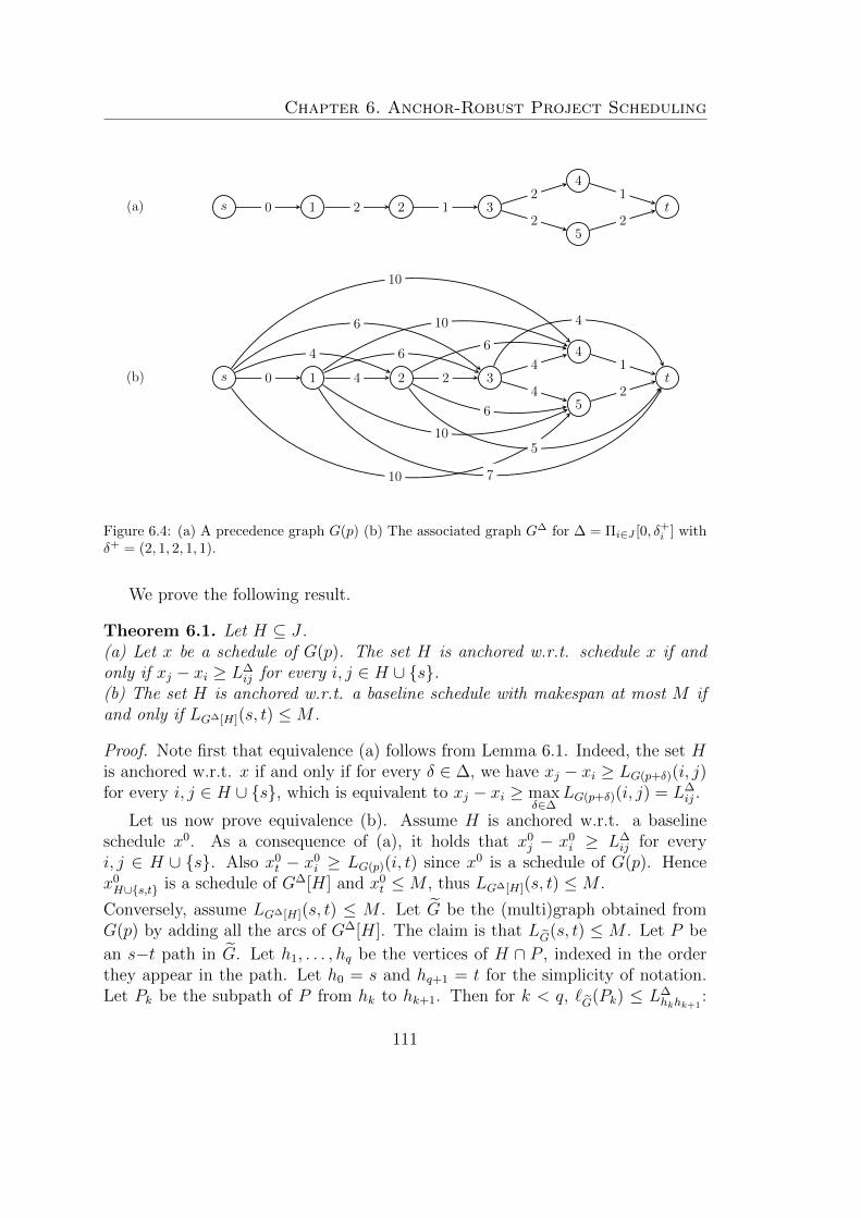
Chapter 6. Anchor-Robust Project Scheduling
(a) s 1 2 3
4
5
t0 2 12 1
2 2
(b) s 1 2 3
4
5
t0 4 24 1
4 2
4
6
10
10
6
10
10
7
6
6
5
4
Figure 6.4: (a) A precedence graph G(p) (b) The associated graph G∆ for ∆ = Πi∈J [0, δ+i ] with
δ+ = (2, 1, 2, 1, 1).
We prove the following result.
Theorem 6.1. Let H ⊆ J .(a) Let x be a schedule of G(p). The set H is anchored w.r.t. schedule x if andonly if xj − xi ≥ L∆
ij for every i, j ∈ H ∪ {s}.(b) The set H is anchored w.r.t. a baseline schedule with makespan at most M ifand only if LG∆[H](s, t) ≤M .
Proof. Note first that equivalence (a) follows from Lemma 6.1. Indeed, the set His anchored w.r.t. x if and only if for every δ ∈ ∆, we have xj − xi ≥ LG(p+δ)(i, j)for every i, j ∈ H ∪ {s}, which is equivalent to xj − xi ≥ max
δ∈∆LG(p+δ)(i, j) = L∆
ij .
Let us now prove equivalence (b). Assume H is anchored w.r.t. a baselineschedule x0. As a consequence of (a), it holds that x0
j − x0i ≥ L∆
ij for everyi, j ∈ H ∪ {s}. Also x0
t − x0i ≥ LG(p)(i, t) since x0 is a schedule of G(p). Hence
x0H∪{s,t} is a schedule of G∆[H] and x0
t ≤M , thus LG∆[H](s, t) ≤M .
Conversely, assume LG∆[H](s, t) ≤ M . Let G be the (multi)graph obtained fromG(p) by adding all the arcs of G∆[H]. The claim is that LG(s, t) ≤ M . Let P be
an s−t path in G. Let h1, . . . , hq be the vertices of H ∩ P , indexed in the orderthey appear in the path. Let h0 = s and hq+1 = t for the simplicity of notation.Let Pk be the subpath of P from hk to hk+1. Then for k < q, `G(Pk) ≤ L∆
hkhk+1:
111
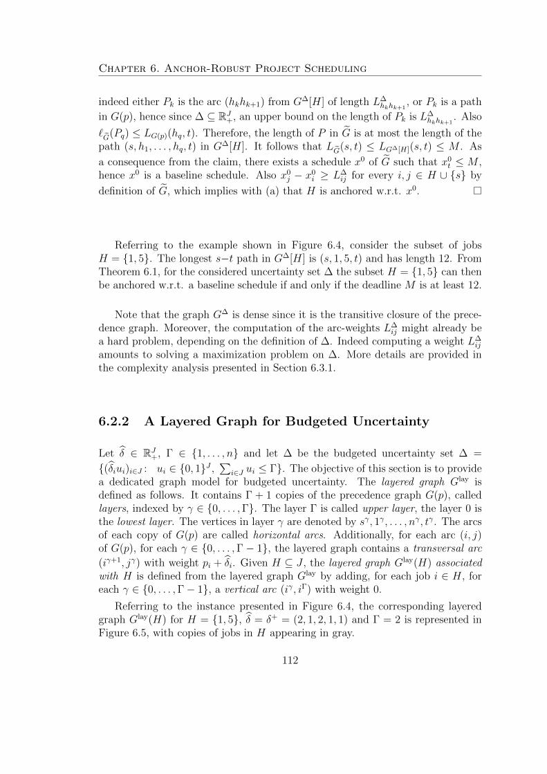
Chapter 6. Anchor-Robust Project Scheduling
indeed either Pk is the arc (hkhk+1) from G∆[H] of length L∆hkhk+1
, or Pk is a path
in G(p), hence since ∆ ⊆ RJ+, an upper bound on the length of Pk is L∆
hkhk+1. Also
`G(Pq) ≤ LG(p)(hq, t). Therefore, the length of P in G is at most the length of thepath (s, h1, . . . , hq, t) in G∆[H]. It follows that LG(s, t) ≤ LG∆[H](s, t) ≤ M . As
a consequence from the claim, there exists a schedule x0 of G such that x0t ≤ M ,
hence x0 is a baseline schedule. Also x0j − x0
i ≥ L∆ij for every i, j ∈ H ∪ {s} by
definition of G, which implies with (a) that H is anchored w.r.t. x0.
Referring to the example shown in Figure 6.4, consider the subset of jobsH = {1, 5}. The longest s−t path in G∆[H] is (s, 1, 5, t) and has length 12. FromTheorem 6.1, for the considered uncertainty set ∆ the subset H = {1, 5} can thenbe anchored w.r.t. a baseline schedule if and only if the deadline M is at least 12.
Note that the graph G∆ is dense since it is the transitive closure of the prece-dence graph. Moreover, the computation of the arc-weights L∆
ij might already bea hard problem, depending on the definition of ∆. Indeed computing a weight L∆
ij
amounts to solving a maximization problem on ∆. More details are provided inthe complexity analysis presented in Section 6.3.1.
6.2.2 A Layered Graph for Budgeted Uncertainty
Let δ ∈ RJ+, Γ ∈ {1, . . . , n} and let ∆ be the budgeted uncertainty set ∆ =
{(δiui)i∈J : ui ∈ {0, 1}J ,∑
i∈J ui ≤ Γ}. The objective of this section is to providea dedicated graph model for budgeted uncertainty. The layered graph Glay isdefined as follows. It contains Γ + 1 copies of the precedence graph G(p), calledlayers, indexed by γ ∈ {0, . . . ,Γ}. The layer Γ is called upper layer, the layer 0 isthe lowest layer. The vertices in layer γ are denoted by sγ, 1γ, . . . , nγ, tγ. The arcsof each copy of G(p) are called horizontal arcs. Additionally, for each arc (i, j)of G(p), for each γ ∈ {0, . . . ,Γ − 1}, the layered graph contains a transversal arc
(iγ+1, jγ) with weight pi + δi. Given H ⊆ J , the layered graph Glay(H) associatedwith H is defined from the layered graph Glay by adding, for each job i ∈ H, foreach γ ∈ {0, . . . ,Γ− 1}, a vertical arc (iγ, iΓ) with weight 0.
Referring to the instance presented in Figure 6.4, the corresponding layeredgraph Glay(H) for H = {1, 5}, δ = δ+ = (2, 1, 2, 1, 1) and Γ = 2 is represented inFigure 6.5, with copies of jobs in H appearing in gray.
112
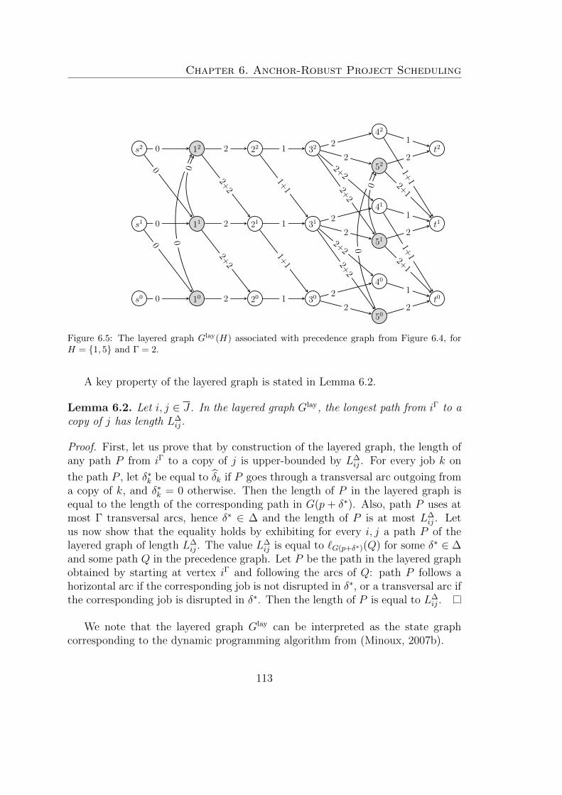
Chapter 6. Anchor-Robust Project Scheduling
s0 20 30
40
t010
50
s1 21 31
41
t111
51
s2 22 32
42
t212
52
0 2 12 1
2 2
0 2 12 1
2 2
0 2 12 1
2 2
0
2+2
1+1
2+2
1+1
2+2
2+1
0
2+2
1+1
2+2
1+1
2+2
2+1
0
0
0
0
Figure 6.5: The layered graph Glay(H) associated with precedence graph from Figure 6.4, forH = {1, 5} and Γ = 2.
A key property of the layered graph is stated in Lemma 6.2.
Lemma 6.2. Let i, j ∈ J . In the layered graph Glay, the longest path from iΓ to acopy of j has length L∆
ij .
Proof. First, let us prove that by construction of the layered graph, the length ofany path P from iΓ to a copy of j is upper-bounded by L∆
ij . For every job k on
the path P , let δ∗k be equal to δk if P goes through a transversal arc outgoing froma copy of k, and δ∗k = 0 otherwise. Then the length of P in the layered graph isequal to the length of the corresponding path in G(p + δ∗). Also, path P uses atmost Γ transversal arcs, hence δ∗ ∈ ∆ and the length of P is at most L∆
ij . Letus now show that the equality holds by exhibiting for every i, j a path P of thelayered graph of length L∆
ij . The value L∆ij is equal to `G(p+δ∗)(Q) for some δ∗ ∈ ∆
and some path Q in the precedence graph. Let P be the path in the layered graphobtained by starting at vertex iΓ and following the arcs of Q: path P follows ahorizontal arc if the corresponding job is not disrupted in δ∗, or a transversal arc ifthe corresponding job is disrupted in δ∗. Then the length of P is equal to L∆
ij .
We note that the layered graph Glay can be interpreted as the state graphcorresponding to the dynamic programming algorithm from (Minoux, 2007b).
113
Chapter 6. Anchor-Robust Project Scheduling
Theorem 6.2. Let ∆ be a budgeted uncertainty set. Let H ⊆ J .(a) Let z be a schedule of G(p). The set H is anchored w.r.t. schedule z if andonly if there exists a schedule x of Glay(H) such that xΓ
i = zi for every i ∈ J .(b) A set H is anchored w.r.t. a baseline schedule with makespan at most M ifand only if LGlay(H)(s
Γ, tΓ) ≤M .
Proof. (a) Assume the set H is anchored w.r.t. z, or equivalently with Theo-rem 6.1, that zj − zi ≥ L∆
ij for every i, j ∈ H ∪ {s}. Let us prove that zj − zi ≥LGlay(H)(i
Γ, jΓ) for every i, j ∈ J : indeed by Lemma 6.1 it is a sufficient condition
for the existence of a schedule x of Glay(H) such that xΓi = zi for every i ∈ J .
Let P be an iΓ−jΓ path in Glay(H), and let h1, . . . , hq be the jobs of H corre-sponding to vertical arcs of P . Let h0 = i and hq+1 = j for the ease of notation.Consider Pk, k ∈ {0, . . . , q} the subpath of P going from hΓ
k to a copy of hk+1.By definition of the hk’s the path Pk uses no vertical arc: it is a path in Glay. ByLemma 6.2, it comes `Glay(H)(Pk) ≤ L∆
hkhk+1. By assumption on z it holds that
L∆hkhk+1
≤ zhk+1− zhk , hence `Glay(H)(Pk) ≤ zhk+1
− zhk . Summing up the inequalityover k ∈ {0, . . . , q} we obtain `Glay(H)(P ) ≤ zhq+1 − zh0 = zj − zi. This holds forevery iΓ−jΓ path P , therefore zj − zi ≥ LGlay(H)(i
Γ, jΓ).Conversely, assume the existence of such a schedule x. Let us prove that zj − zi ≥L∆ij for every i, j ∈ H ∪ {s}. Let i, j ∈ H ∪ {s}, and consider γ ∈ {0, . . . ,Γ} such
that there is a path from iΓ to jγ which is a longest path between iΓ and a copyof j in Glay. Then zj − zi = xΓ
j − xΓi = xΓ
j − xγj + xγj − xΓ
i , where xΓj − x
γj ≥ 0
because of the vertical arc (jγ, jΓ), and xγj − xΓi ≥ L∆
ij by definition of γ and withLemma 6.2. Thus zj−zi ≥ L∆
ij and with Theorem 6.1, the set H is anchored w.r.t.z.
Equivalence (b) can then be proven as follows. From (a), a subset H is anchoredw.r.t. a baseline schedule if and only if there exists a schedule of Glay(H) whoserestriction to the upper layer has makespan at most M . The existence of such aschedule is equivalent to LGlay(H)(s
Γ, tΓ) ≤M .
Referring to the layered graph represented in Figure 6.5, the longest s2−t2path is (s2, 12, 21, 31, 50, 52, t2), with length 11. From Theorem 6.2, for uncertaintybudget Γ = 2, the subset H = {1, 5} can be anchored w.r.t. a baseline schedule ifand only if the deadline M is at least 11.
Let us now derive a compact mixed integer programming (MIP) formulationfor AnchRobPSP under budgeted uncertainty, using the layered graph. A realvariable xγj ≥ 0 is associated with every vertex jγ of the layered graph; a binaryvariable hj ∈ {0, 1} is associated with every job j ∈ J , so that hj = 1 if j isanchored, and hj = 0 otherwise. Let A denote the arc-set of the precedence graphG. Let Dj = LG(p+δ)(s, j) − LG(p)(s, j) for every j ∈ J . Consider the followingprogram.
114

Chapter 6. Anchor-Robust Project Scheduling
(Lay) max∑i∈J
aihi
s.t. xγj − xγi ≥ pi ∀(i, j) ∈ A, ∀γ ∈ {0, . . . ,Γ} (1)
xγj − xγ+1i ≥ pi + δi ∀(i, j) ∈ A, ∀γ ∈ {0, . . . ,Γ− 1} (2)
xΓj − x
γj ≥ −Dj(1− hj) ∀j ∈ J , ∀γ ∈ {0, . . . ,Γ− 1} (3)
xΓt ≤M (4)
xγj ≥ 0 ∀j ∈ J, ∀γ ∈ {0, . . . ,Γ}
hj ∈ {0, 1} ∀j ∈ J
Theorem 6.3. Program (Lay) is a valid MIP formulation for AnchRobPSP underuncertainty budget Γ.
Proof. With Theorem 6.2, AnchRobPSP is equivalent to maximizing a(H) subjectto H ⊆ J , x schedule of Glay(H), xΓ
t ≤ M . Let us show that there exists afeasible pair (x,H) of the problem with objective value a(H) if and only if thereexists a feasible solution of program (Lay) with objective value equal to a(H).First note that, given a feasible solution (x, h) of the MIP, it holds that x isa schedule of Glay(H) where H = {i ∈ J : hi = 1}. Indeed constraints (1)and (2) correspond to horizontal and transversal arcs respectively, and constraints(3) correspond to vertical arcs for jobs i ∈ H. Conversely, consider H ⊆ Jsuch that there exists a schedule x of Glay(H), xΓ
t ≤ M . Let x′ be the earliestschedule of Glay(H). Note that x′Γt ≤ M . Let h be the indicator vector of H.Then (x′, h) is a feasible solution of the MIP with objective value a(H). Indeedx′ clearly satisfies constraints (1)-(2)-(4), and constraint (3) when hj = 1. Itremains to prove that x′ also satisfies constraint (3) when hj = 0. We havex′γj = LGlay(H)(s
Γ, jγ) ≤ LGlay(J)(sΓ, jγ) ≤ LG(p+δ)(s, j). Indeed in Glay(J) the
longest sΓ−jγ path uses alternatively vertical and transversal arcs, hence its lengthis the length of the corresponding s−j path in G(p + δ). Also x′Γj ≥ LG(p)(s, j),
hence x′γj − x′Γj ≤ LG(p+δ)(s, j)− LG(p)(s, j) = Dj.
Note that the values Dj can be computed in polynomial time in a preprocessingstep.
Theorem 6.3 thus provides a compact MIP formulation for AnchRobPSP un-der budgeted uncertainty, with a linear number of binary variables, a polynomialnumber of continuous variables and a polynomial number of constraints. Note alsothat program (Lay) can readily be modified to tackle A-AnchRobPSP, by settingminxΓ
t in the objective and adding constraint∑
i∈J aihi ≥ A instead of (4). It
115
Chapter 6. Anchor-Robust Project Scheduling
is important to emphasize that a compact formulation is not a general rule forrobust 2-stage problems but rather an exception. For static-robust problems suchformulations were key results of the work of (Soyster, 1973) and (Bertsimas andSim, 2004). Both AnchRobPSP and A-AnchRobPSP for budgeted uncertainty canthus be readily solved with an off-the-shelf MIP solver.
6.3 Complexity of the Anchor-Robust Project
Scheduling Problem
To study the complexity of AnchRobPSP, we consider two distinct complexityissues, depending on whether the inputs of the problem contain G(p) and ∆, ordirectly the graph G∆ with the arc-weights L∆
ij . On the one hand, if the values L∆ij
are part of the input, the decision version of AnchRobPSP is in NP, since checkingwhether LG∆[H](s, t) ≤ M can be done in polynomial time. On the other hand, ifthe values L∆
ij are not part of the input, we show that for some uncertainty setsit is co-NP-complete to decide if a set H is anchored, and thus AnchRobPSP isco-NP-hard. Let us start with this latter point.
6.3.1 AnchRobPSP is at least as hard as computing L∆ij
LetD be a family of uncertainty sets. Let Worst-case Longest Path WLP(D)be the following problem: given a precedence graph G(p), a job j ∈ J , ∆ ∈ D,L ≥ 0, is it true that for every δ ∈ ∆, the longest s−j path in G(p + δ) haslength at most L? Note that this problem is to decide whether L∆
sj ≤ L. Let alsoAnch(D) be the decision version of AnchRobPSP over the family of uncertaintysets D, that is: given a precedence graph G(p), ∆ ∈ D, M ≥ 0, a ∈ RJ
+, A ≥ 0, isthere H ⊆ J such that a(H) ≥ A and LG∆[H](s, t) ≤M?
Lemma 6.3. There exists a polynomial reduction from WLP(D) to Anch(D).
Proof. Let IWLP = (G(p), j,∆, L) be an instance of WLP(D). An associatedinstance IA = (G′(p′),∆′,M ′, a′, A′) of Anch(D) problem is built as follows. LetG′ = G, and p′i = pi if job i is a predecessor of j, and p′i = 0 otherwise (includingp′j = 0). Let M ′ = L and ∆′ = ∆. Finally let a′i = 1 for every i 6= j, anda′j = A′ = n, where n is the number of jobs in G(p).
For instance IA, the anchoring weights are such that a subset H of jobs satisfiesa′(H) ≥ A′ if and only if it contains job j. If IWLP has a ‘yes’ answer, i.e., ifL∆sj ≤ L, then LG′∆′ [{j}](s, t) = L∆
sj + LG′(p′)(j, t) ≤ L = M ′. Thus the singleton{j} yields a ‘yes’ answer for IA. Conversely, if H is anchored and a′(H) ≥ A′,
116
Chapter 6. Anchor-Robust Project Scheduling
then j ∈ H. The value L∆sj is the arc-weight of the arc (s, j) of G′∆
′[H], hence
L∆sj ≤ LG′∆′ [H](s, t) ≤M ′ = L.
Note that the reduction can be modified so that anchoring weights are all equalto one in IA. Indeed it suffices to replace job j by n duplicates of j, all with thesame predecessors and successors as j. The reduction then applies similarly.
Let us fix notation for the Knapsack problem in order to show the followingtheorem. The Knapsack problem is: given a set I of m items, w ∈ NI , v ∈ NI ,W ∈ N, V ∈ N, is there a subset S ⊆ I of items such that w(S) ≤ W andv(S) ≥ V .
Theorem 6.4. AnchRobPSP is co-NP-hard for upper-bounded uncertainty sets,even with unit anchoring weights.
Proof. We claim that the complement of WLP(D) is NP-hard when D denotes
the family of sets ∆ defined by ∆ ={
(δiui)i∈J : ui ∈ {0, 1}J ,∑
i∈J αiui ≤ β}
for
some α ∈ NJ and β ∈ N. Every ∆ of that form is an upper-bounded uncertaintyset. From the reduction of Lemma 6.3, the claim will imply that AnchRobPSPis co-NP-hard in this case. Let us now show this claim. The complement ofWLP(D) is: given G(p), job j, set ∆ defined by δ, α, β, and L ≥ 0, is there u ∈{0, 1}J such that
∑i∈J αiui ≤ β and LG(p+δu)(s, j) > L? The proof is a reduction
from Knapsack. Let IKP = (I = {1, . . . ,m}, wi, vi,W, V ) be an instance of
the Knapsack problem. The associated instance IWLP = (G(p), j, δ, α, β, L) ofWLP(D) is defined as follows. Let L = V −1, let G(p) be a path (s, 1, . . . ,m, j, t)
with arc-weights pi = 0 for every i ∈ I, pj = 0. Let δi = vi, αi = wi for everyi ∈ I, and β = W . Given u ∈ {0, 1}J , the constraint
∑i∈J αiui ≤ β then writes∑
i∈I wiui ≤ W , and LG(p+δu)(s, j) =∑
i∈I(pi + δiui) =∑
i∈I viui. Hence there
exists u ∈ {0, 1}J that yields a ‘yes’ answer for the complement of WLP(D) onIWLP if and only if it yields a ‘yes’ answer for the instance IKP of the Knapsackproblem.
6.3.2 NP-Completeness for Budgeted Uncertainty
In this section we show that for DΓ the family of budgeted uncertainty sets, thedecision version Anch(DΓ) of AnchRobPSP is NP-complete. First note that forevery ∆ ∈ DΓ the values L∆
ij can be computed in polynomial time by the dynamicprogramming algorithm from (Minoux, 2007b). Hence Anch(DΓ) is in NP.
We establish the following lemma when the precedence graph is a path.
Lemma 6.4. Let G be an s−t path (s, 1, 2, . . . , n, t). A subset {h1, . . . , hq} ⊆J (with h1 < · · · < hq) is anchored w.r.t. a baseline schedule if and only ifL∆sh1
+ L∆h1h2
+ · · ·+ L∆hq−1hq
+ LG(p)(hq, t) ≤M .
117
Chapter 6. Anchor-Robust Project Scheduling
Proof. We show that L∆ij ≤ L∆
ik + L∆kj for every i ≤ k ≤ j. Indeed if Pij denotes
the (unique) i−j path in G, for some δ∗ ∈ ∆ it holds that L∆ij = `G(p+δ∗)(Pij) =
`G(p+δ∗)(Pik) + `G(p+δ∗)(Pkj) ≤ L∆ik + L∆
kj. This inequality implies that the longests−t path in G∆[H] is the path (s = h0, h1, . . . , hq, t = hq+1) going through all jobsof H. The result follows from Theorem 6.1.
Theorem 6.5. Anch(DΓ) is NP-complete, even if Γ = 1 and the precedence graphis a path.
Proof. The proof is a reduction from Knapsack. The problem Anch(DΓ) ona path with Γ = 1 is stated as follows: given a precedence graph G(p) which is
an s−t path, δ ∈ RJ+, M ≥ 0, a ∈ RJ
+, A ≥ 0, is there a subset H ⊆ J suchthat a(H) ≥ A and LG∆[H](s, t) ≤ M , where ∆ is the budgeted uncertainty set
defined by δ and Γ = 1. Let IKP = (I = {1, . . . ,m}, wi, vi,W, V ) be an instance
of the Knapsack problem. The associated instance IA = (J, pi, δ,M, ai, A) ofAnch(DΓ) is as follows:• the set of jobs is J = {0, 1, . . . ,m,m+ 1}, where we assume w.l.o.g. that the
items 1, . . . ,m are sorted by decreasing weight: w1 ≥ · · · ≥ wm• the precedence graph is the path (0, 1, . . . ,m+ 1) and pi = 0 for every i ∈ J• δi = wi for every i ∈ I, δ0 = 1 + max
i∈Iwi, δm+1 = 0 (hence δ0 ≥ δ1 ≥ · · · ≥
δm+1)
• M = W + δ0
• ai = vi for every i ∈ I, a0 = 0, am+1 = v where v = 1 +∑
i∈I vi• A = V + vThe size of IA is polynomial in the size of IKP . We prove three claims on the
instance IA.(i) Let H ⊆ J and S = H∩I. Then a(H) ≥ A ⇐⇒ v(S) ≥ V and m+1 ∈ H.
Indeed a(H) ≥ A writes v(S)+ v1m+1∈H ≥ V + v. If m+1 /∈ H then the inequalitycannot be satisfied since v > v(S).
(ii) For every i, j ∈ J such that i < j, L∆ij = δi and L∆
si = δ0. Indeed by
definition L∆ij = maxδ∈∆
∑i≤k<j δk = maxi≤k<j δk which equals δi if i 6= s and δ0
otherwise.(iii) Let H ⊆ J such that m + 1 ∈ H and let S = H ∩ I. Then LG∆[H](s, t) ≤
M ⇐⇒ w(S) ≤ W . Let H = {h1, . . . , hq} with h1 < · · · < hq. By Lemma 6.4
and claim (ii), LG∆[H](s, t) = δ0 + δh1 + · · · + δhq−1 . Note that S = {h1, . . . , hq−1}since m+ 1 ∈ H. Thus LG∆[H](s, t) ≤M ⇐⇒ δ0 + δ(S) ≤M ⇐⇒ w(S) ≤ W .
Let us now prove that the instance IKP of the Knapsack problem has a ‘yes’answer if and only if the instance IA of Anch(DΓ) has a ‘yes’ answer. If thereexists some S ⊆ I such that w(S) ≤ W and v(S) ≥ V , then let H = S ∪ {m+ 1}:by (i) it comes a(H) ≥ A, and by (iii) LG∆[H](s, t) ≤M . Conversely assume there
118
Chapter 6. Anchor-Robust Project Scheduling
exists H ⊆ J such that a(H) ≥ A and LG∆[H](s, t) ≤M , and let S = H ∩ I. Thenby (i) v(S) ≥ V and m + 1 ∈ H, and by (iii) w(S) ≤ W . Hence the problemAnch(DΓ) is NP-complete, even if the precedence graph is a path and Γ = 1.
Now consider the case where δ is uniform, i.e., δi = δ0 for every i ∈ J for someδ0 ∈ R+.
Theorem 6.6. Anch(DΓ) is NP-complete, even if Γ = 1 and δ is uniform.
Proof. Let IKP = (I = {1, . . . ,m}, wi, vi,W, V ) be a Knapsack instance. Let
us build an instance IA = (n,G, p, δ0,M, a, A) of Anch(DΓ) as follows. An illus-tration is given in Figure 6.6, where the instance is represented, with processingtimes on arcs and anchoring weights in brackets.• Let n = 3m+ 1. Jobs are j1, . . . , jm+1, α1, . . . , αm, β1, . . . , βm.• The precedence graph is as follows: job ji, i ≤ m has two successors αi andβi; job αi has successor job ji+1; job βi has successor job ji+1.• Let processing times be defined by: pji = 1 for every i ≤ m; pjm+1 = 0;pβi = 1 for every i ≤ m; pαi = 1 + wmax − wi for every i ≤ m, wherewmax = maxi∈I wi.• Let δ0 = wmax.• Let M = 2m(1 + δ0)−
∑i∈I wi +W .
• With vtot =∑
i∈I vi, let aji = vtot for every i ≤ m + 1, aαi = 0 and aβi = vifor every i ≤ m.• Finally A = (m+ 1)vtot + V .Given a subset of jobs H, it comes that a(H) =
∑i:ji∈H vtot +
∑i:βi∈H vi.
Hence, setting S := {i : βi ∈ H}, we have a(H) = |{i : ji ∈ H}|vtot + v(S). Hencea(H) ≥ A if and only if all ji’s are in H and v(S) ≥ V .
Consider a subset H of jobs that contains all ji’s, but no αi. Let us nowcompute LG∆[H](s, t) in this instance. Fix i ≤ m. Let us compute LG∆[H](ji, ji+1).Case 1. If βi ∈ H, the path through αi has worst-case length 2 + wmax − wi +δ0, the path through βi has worst-case length 2 + 2δ0. Hence since δ0 = wmax,LG∆[H](ji, ji+1) = 2 + 2δ0.
Case 2. If βi /∈ H, the path through αi has worst-case length 2 + wmax − wi + δ0,the path through βi has worst-case length 2 + δ0. Hence LG∆[H](ji, ji+1) = 2 +
wmax − wi + δ0.We now prove that IKP has a ‘yes’ answer if and only if IA has a ‘yes’ answer.
Assume there exists S a solution to the knapsack problem for IKP . Consider thesubset of jobs H = {ji, i ≤ m + 1} ∪ {βi, i ∈ S}. Then a(H) ≥ A, as notedpreviously. Consider now the longest s−t path in G∆[H]. We claim that w.l.o.g.such a longest path goes through every job ji, i ≤ m + 1. Consider some job jiand let u (resp. v) be a job before ji (resp. after ji) in the precedence graph.
119
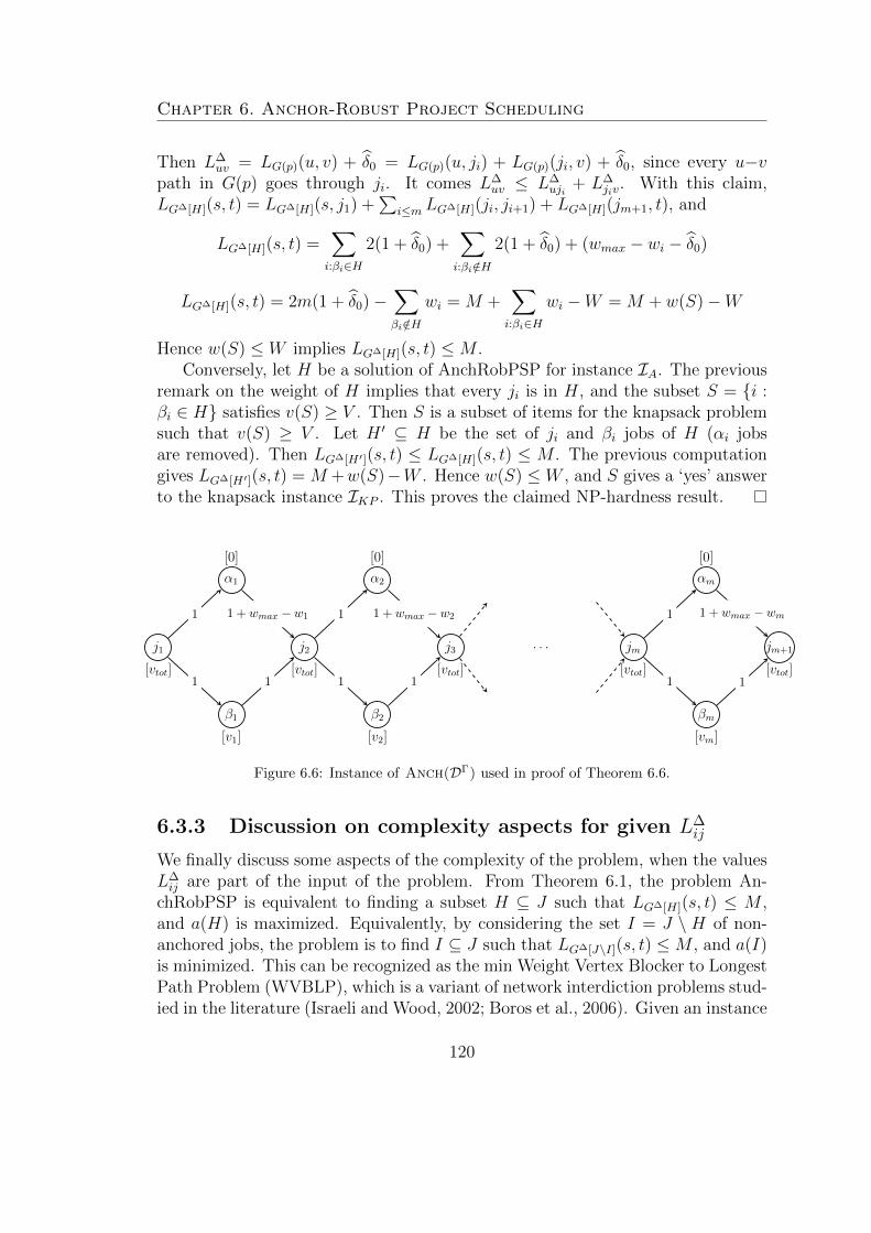
Chapter 6. Anchor-Robust Project Scheduling
Then L∆uv = LG(p)(u, v) + δ0 = LG(p)(u, ji) + LG(p)(ji, v) + δ0, since every u−v
path in G(p) goes through ji. It comes L∆uv ≤ L∆
uji+ L∆
jiv. With this claim,
LG∆[H](s, t) = LG∆[H](s, j1) +∑
i≤m LG∆[H](ji, ji+1) + LG∆[H](jm+1, t), and
LG∆[H](s, t) =∑i:βi∈H
2(1 + δ0) +∑i:βi /∈H
2(1 + δ0) + (wmax − wi − δ0)
LG∆[H](s, t) = 2m(1 + δ0)−∑βi /∈H
wi = M +∑i:βi∈H
wi −W = M + w(S)−W
Hence w(S) ≤ W implies LG∆[H](s, t) ≤M .Conversely, let H be a solution of AnchRobPSP for instance IA. The previous
remark on the weight of H implies that every ji is in H, and the subset S = {i :βi ∈ H} satisfies v(S) ≥ V . Then S is a subset of items for the knapsack problemsuch that v(S) ≥ V . Let H ′ ⊆ H be the set of ji and βi jobs of H (αi jobsare removed). Then LG∆[H′](s, t) ≤ LG∆[H](s, t) ≤ M . The previous computationgives LG∆[H′](s, t) = M +w(S)−W . Hence w(S) ≤ W , and S gives a ‘yes’ answerto the knapsack instance IKP . This proves the claimed NP-hardness result.
j1
α1
β1
j2
α2
β2
j3 jm
αm
βm
jm+1
1
1 1
1 + wmax − w1 1
1 1
1 + wmax − w2 1
1 1
1 + wmax − wm
. . .
[vtot]
[0]
[v1]
[vtot]
[0]
[v2]
[vtot] [vtot]
[0]
[vm]
[vtot]
Figure 6.6: Instance of Anch(DΓ) used in proof of Theorem 6.6.
6.3.3 Discussion on complexity aspects for given L∆ij
We finally discuss some aspects of the complexity of the problem, when the valuesL∆ij are part of the input of the problem. From Theorem 6.1, the problem An-
chRobPSP is equivalent to finding a subset H ⊆ J such that LG∆[H](s, t) ≤ M ,and a(H) is maximized. Equivalently, by considering the set I = J \ H of non-anchored jobs, the problem is to find I ⊆ J such that LG∆[J\I](s, t) ≤M , and a(I)is minimized. This can be recognized as the min Weight Vertex Blocker to LongestPath Problem (WVBLP), which is a variant of network interdiction problems stud-ied in the literature (Israeli and Wood, 2002; Boros et al., 2006). Given an instance
120
Chapter 6. Anchor-Robust Project Scheduling
of a maximization problem on a network, vertex blocker problems look for a subsetof vertices to remove, so that the optimum of the maximization problem in theremaining graph falls below a given threshold. Hence AnchRobPSP correspondsto WVBLP on G∆, thus raising the question of the complexity of the WVBLP onG∆ graphs. Many vertex blocker problems have been shown to be NP-complete(Boros et al., 2006), but these results cannot be directly applied to AnchRobPSP,since it is the restriction of WVBLP to very structured instances, namely the G∆
graphs. Recall that the G∆ are transitive closures of directed acyclic graphs, andtheir arc-weights are values L∆
ij and LG(p)(j, t). Theorem 6.5 provides an NP-hardcase of the problem WVBLP on G∆ instances. Note that the reduction involvesnon-unit anchoring weights. The complexity of AnchRobPSP when the values L∆
ij
are part of the input, and with unit anchoring weights, is still an open question.
6.4 Algorithms for special cases of
AnchRobPSP
In this section we provide an algorithm (Algorithm A+) to compute a feasiblesolution for AnchRobPSP under upper-bounded uncertainty, and show that An-chRobPSP under box uncertainty is a polynomial case where Algorithm A+ isexact. For budgeted uncertainty, polynomial algorithms are exhibited for spe-cial cases, and a dynamic programming approach is proposed for series-parallelprecedence graphs.
6.4.1 Algorithm A+ for upper-bounded uncertainty
In this section the set ∆ is an upper-bounded uncertainty set, i.e., there existsδ+ ∈ RJ
+ such that δ+i ≥ δi for every i ∈ J for every δ ∈ ∆. Let x denote the
earliest schedule of G(p + δ+). A first remark is that if the makespan of x is atmost M , then (x, J) is an optimal solution of AnchRobPSP. Indeed x is then botha baseline schedule and a feasible second-stage schedule for every δ ∈ ∆, since δ+
is an upper bound on ∆. However, in general the makespan of x is larger than Mand then not all jobs can be anchored. Let x denote the latest schedule of G(p)such that xt = M . Consider the following algorithm.
121
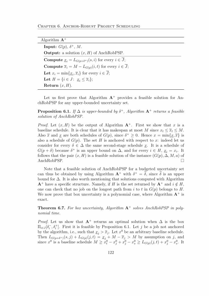
Chapter 6. Anchor-Robust Project Scheduling
Algorithm A+
Input: G(p), δ+, M .
Output: a solution (x,H) of AnchRobPSP.
Compute xi = LG(p+δ+)(s, i) for every i ∈ J ;
Compute xi = M − LG(p)(i, t) for every i ∈ J ;
Let xi = min{xi, xi} for every i ∈ J ;
Let H = {i ∈ J : xi ≤ xi};Return (x,H).
Let us first prove that Algorithm A+ provides a feasible solution for An-chRobPSP for any upper-bounded uncertainty set.
Proposition 6.1. If ∆ is upper-bounded by δ+, Algorithm A+ returns a feasiblesolution of AnchRobPSP.
Proof. Let (x,H) be the output of Algorithm A+. First we show that x is abaseline schedule. It is clear that it has makespan at most M since xt ≤ xt ≤M .Also x and x are both schedules of G(p), since δ+ ≥ 0. Hence x = min{x, x} isalso a schedule of G(p). The set H is anchored with respect to x: indeed let usconsider for every δ ∈ ∆ the same second-stage schedule x. It is a schedule ofG(p + δ) because δ+ is an upper bound on ∆, and for every i ∈ H, xi = xi. Itfollows that the pair (x,H) is a feasible solution of the instance (G(p),∆,M, a) ofAnchRobPSP.
Note that a feasible solution of AnchRobPSP for a budgeted uncertainty setcan thus be obtained by using Algorithm A+ with δ+ = δ, since δ is an upperbound for ∆. It is also worth mentioning that solutions computed with AlgorithmA+ have a specific structure. Namely, if H is the set returned by A+ and i /∈ H,one can check that no job on the longest path from i to t in G(p) belongs to H.We now prove that box uncertainty is a polynomial case, where Algorithm A+ isexact.
Theorem 6.7. For box uncertainty, Algorithm A+ solves AnchRobPSP in poly-nomial time.
Proof. Let us show that A+ returns an optimal solution when ∆ is the boxΠi∈J [δ−i , δ
+i ]. First it is feasible by Proposition 6.1. Let j be a job not anchored
by the algorithm, i.e., such that xj > xj. Let x0 be an arbitrary baseline schedule.Then LG(p+δ+)(s, j) + LG(p)(j, t) = xj + M − xj > M by assumption on j, andsince x0 is a baseline schedule M ≥ x0
t − x0j + x0
j − x0s ≥ LG(p)(j, t) + x0
j − x0s. It
122
Chapter 6. Anchor-Robust Project Scheduling
comes LG(p+δ+)(s, j) > x0j − x0
s. From Lemma 6.1, there exists no schedule xδ+
of
G(p + δ+) such that xδ+
j = x0j . Since δ+ ∈ ∆, job j cannot be in any anchored
set. Since all anchoring weights are non-negative, the solution returned by thealgorithm is optimal.
Note that the proof only requires that ∆ is upper-bounded by δ+ and thatδ+ ∈ ∆, which is more general than ∆ being the box Πi∈J [δ−i , δ
+i ]. The proof of
Theorem 6.7 also yields as a corollary that the set H optimal for AnchRobPSPunder box uncertainty is unique, and it is the set returned by Algorithm A+.
Interestingly, for box uncertainty it can be shown that the proactive problemDAPSP of (Bendotti et al., 2017) and AnchRobPSP coincide. The analysis ofAlgorithm A+ thus yields a simpler proof of the polynomiality of DAPSP forbox uncertainty. Moreover, the algorithm proposed in (Bendotti et al., 2017) hascomplexity O(n3), while Algorithm A+ is linear in the number of arcs in G.
6.4.2 Polynomial Cases for Budgeted Uncertainty
Under budgeted uncertainty, AnchRobPSP is NP-hard as shown in Theorem 6.5.In this section we exhibit polynomial special cases.
6.4.2.1 Path precedence graph and unit anchoring weights.
We first investigate the case where the precedence graph is a path. The reduc-tion from Theorem 6.5 relies on the numerical values of anchoring weights. Weshow that in the case of unit anchoring weights the problem becomes solvable inpolynomial time.
Theorem 6.8. Let G be an s−t path, and let ∆ be a budgeted uncertainty set. Ifai = 1 for every i ∈ J , then AnchRobPSP is solvable in polynomial time.
Proof. Under budgeted uncertainty, the arc-weights of graph G∆ can be computedin polynomial time. Consider then the problem of finding an s−t path in G∆ withlength at most M , and with a maximum number of arcs. This problem is solvablein polynomial time as a polynomial case of the Resource-Constrained Longest PathProblem (Garey and Johnson, 1979). The claim is that this problem is equivalentto solving the special case of AnchRobPSP. Indeed from Lemma 6.4, there is aone-to-one correspondance between subsets of jobs and s−t paths in G∆, and asubset H is feasible for AnchRobPSP if and only if the corresponding path haslength at most M in G∆. Hence maximizing a(H) = |H| amounts to maximizingthe number of arcs in the associated s−t path, under the constraint that the lengthof the path is at most M .
123
Chapter 6. Anchor-Robust Project Scheduling
Note that the result holds not only for budgeted uncertainty, but also for anyuncertainty set for which the arc-weights L∆
ij can be computed in polynomial time.
6.4.2.2 A special case with pi=0, δi=1, Γ=1, ai=1.
Let the precedence graph G be any directed acyclic graph. Let us consider thespecial case U-AnchRobPSP where pi = 0 and ai = 1 for every i ∈ J and ∆ is abudgeted uncertainty with δi = 1 for every i ∈ J and budget Γ = 1. An instanceof U-AnchRobPSP is thus formed with the graph G and the deadline M , assumedto be an integer. We will show that U-AnchRobPSP is a polynomial case, by anequivalence with a poset problem. Recall that a partial order ≺ can be naturallydefined from the precedence graph G by setting i ≺ j if there exists an i−j pathin G. Let MaxSubposet be the problem of finding, given a poset and an integerM , a max-size subposet in which all chains have size at most M .
Let (G,M) be an instance of U-AnchRobPSP, and let J∗ denote the set of jobsthat have a predecessor other than s in the precedence graph G. The arc-weightsof G∆ are as follows: the arcs from s to a job i /∈ J∗ have weight 0, all incomingarcs of t have weight 0, all other arcs have weight 1. Consequently, given H ⊆ J ,the length of an s−t path in G∆[H] is equal to the number of vertices of J∗ inthe path. It follows that LG∆[H](s, t) ≤M if and only if all chains in the subposet(H ∩ J∗,≺) have size at most M . Finally, since G can be any directed acyclicgraph, the poset (J∗,≺) can be any poset. Thus U-AnchRobPSP is equivalent toMaxSubposet.
Theorem 6.9. U-AnchRobPSP is solvable in polynomial time.
Proof. Note first that a subposet in which all chains have size at most M is exactlythe union of M antichains (some of the antichains being possibly empty). Theproblem of finding a max-size union of M antichains in a poset can be solved inpolynomial time, through a min-cost circulation algorithm (see Theorem 14.8 inSchrijver (2003)). Using this result and the equivalence between U-AnchRobPSPand MaxSubposet, the result follows.
6.4.3 Dynamic Programming for Budgeted Uncertaintyand Series-Parallel Precedence Graphs
This section is devoted to solving AnchRobPSP under budgeted uncertainty forseries-parallel precedence graphs. It is assumed that vectors p, δ, and the deadlineM have integer values. Series-parallel digraphs are defined recursively as follows.A digraph is series-parallel with terminals s and t if one of the three assertions issatisfied:
124
Chapter 6. Anchor-Robust Project Scheduling
• Its vertex-set is {s, t} and its arc-set is {(s, t)};• (Series composition.) It is formed with two series-parallel digraphs G1 andG2, where terminals t1 and s2 have been identified;• (Parallel composition.) It is formed with two series-parallel digraphs G1 andG2, where the two pairs of terminals s1 and s2, and t1 and t2, have beenidentified.
In the sequel it is assumed that the precedence graph G is series-parallel withterminals s and t. Given two jobs i and j such that i ≺ j, let Jij denote thesubset of jobs that are successors of i and predecessors of j, with i, j /∈ Jij, i.e.,Jij = {k ∈ J : i ≺ k ≺ j}. Let Gij denote the subgraph of G induced by Jij∪{i, j}:it is series-parallel with terminals i and j.
The proposed algorithmic scheme relies on the layered graph from Section 6.2.2.With Theorem 6.2, a subset H ⊆ J is anchored when there exists a schedule x ofGlay(H) such that xΓ
t ≤ M . Let us now introduce a value function suitable for adynamic programming approach. Given a pair of jobs i, j such that i ≺ j, andb = (bγ)γ∈{0,...,Γ} and b′ = (b′γ)γ∈{0,...,Γ} two vectors of (Γ + 1) integer numbers, thevalue function is
Vij(b, b′) = max a(H)
s.t. H ⊆ Jijx schedule of Glay
ij (H)
xγi = bγ ∀γ ∈ {0, . . . ,Γ}xγj = b′γ ∀γ ∈ {0, . . . ,Γ}
The last two conditions are called boundary conditions in the sequel: theyenforce the values of starting times of copies of i and j in schedule x. LetL = LG(p+δ)(s, t). Let b and b′ be the vectors defined by bγ = 0 for every
γ ∈ {0, . . . ,Γ}, b′Γ = M , and b′γ
= L for every γ ∈ {0, . . . ,Γ− 1}. The maximumweight of an anchored set is then exactly the value Vst(b, b
′). Indeed note thatthe condition xγt ≤ L for every γ ∈ {0, . . . ,Γ − 1} can be added w.l.o.g. By dy-namic programming, the value function will be computed for vectors b, b′ in the setB = {b = (bγ)γ∈{0,...,Γ} : bγ ∈ {0, . . . , L} ∀γ ∈ {0, . . . ,Γ}}. We now show how tocompute the value function in the base case, and prove decomposition propertieswith respect to series and parallel composition.
Lemma 6.5 (Base case.). Let Gij be the digraph with vertex-set {i, j} and arc-set{(i, j)}. Let b, b′ ∈ B. Then Vij(b, b
′) = 0 if b′γ − bγ ≥ pi for every γ ∈ {0, . . . ,Γ}and b′γ − bγ+1 ≥ pi + δi for every γ ∈ {0, . . . ,Γ− 1}. Otherwise Vij(b, b
′) = −∞.
Proof. Note that Jij = ∅, hence the value function is 0 if there exists a schedule
x of Glayij (∅) satisfying the boundary conditions, and −∞ otherwise. Also, the
125
Chapter 6. Anchor-Robust Project Scheduling
boundary conditions fully define the schedule. Hence the value function is 0 ifand only if b and b′ satisfy the constraints of Glay
ij (∅), i.e., b′γ − bγ ≥ pi for every
γ ∈ {0, . . . ,Γ} and b′γ − bγ+1 ≥ pi + δi for every γ ∈ {0, . . . ,Γ− 1}.
Assume Gij is obtained by a parallel composition, w.l.o.g. parallel compositionof two series-parallel digraphs G1
ij and G2ij with terminals i and j. Let J1
ij and J2ij
denote respectively their sets of inner vertices and V 1ij and V 2
ij denote their valuefunctions.
Lemma 6.6 (Parallel composition). For every b, b′ ∈ B, the value function satis-fies Vij(b, b
′) = V 1ij(b, b
′) + V 2ij(b, b
′).
Proof. Let H ⊆ Jij and (H1, H2) be the partition of H defined by H1 = H ∩ J1ij,
H2 = H ∩ J2ij. Given x a schedule of Glay
ij , let x1 (resp. x2) denote the restriction
of x to copies of jobs in G1ij (resp. G2
ij). It holds that x is a schedule of Glayij (H)
such that xi = b and xj = b′ if and only if x1 and x2 are schedules of Glayij (H1)
and Glayij (H2) respectively, and they satisfy x1
i = b and x1j = b′, and x2
i = b andx2j = b′. Hence the value function Vij(b, b
′) decomposes over the subgraphs G1ij and
G2ij, leading to the desired equality.
Assume Gij is obtained by series composition of two series-parallel digraphsGik and Gkj for a given k ∈ Jij.
Lemma 6.7 (Series composition). For every b, b′ ∈ B, the value function satisfies
Vij(b, b′) = max
{maxb′′∈B{Vik(b, b′′) + Vkj(b
′′, b′)} ; ak + maxb′′∈Banch
{Vik(b, b′′) + Vkj(b′′, b′)}
}where Banch = {b ∈ B : bγ ≤ bΓ ∀γ ∈ {0, . . . ,Γ}}.
Proof. Let H ⊆ Jij and let H1 = H ∩ Jik and H2 = H ∩ Jkj. Given x a schedule
of Glayij , let x1 (resp. x2) denote the restriction of x to copies of jobs in Gik (resp.
Gkj). It holds that x is a schedule of Glayij (H) such xi = b and xj = b′ if and only
if: x1 (resp. x2) is a schedule of Glayik (H1) (resp. Glay
kj (H2)), x1k = x2
k = b′′ for some
b′′ ∈ B, and either (i) or (ii) is satisfied: (i) k /∈ H (ii) k ∈ H, b′′ ∈ Banch. Indeedwhen k ∈ H, both schedules x1 and x2 must satisfy the vertical arcs constraints ink, which is equivalent to b′′ ∈ Banch. Case (i) leads to the first term and case (ii)leads to the second term of the maximum; we thus obtain the desired equality.
Theorem 6.10. For fixed uncertainty budget Γ, AnchRobPSP can be solved inO(mL3Γ+3), where m is the number of arcs in the precedence graph and L =LG(p+δ)(s, t).
126
Chapter 6. Anchor-Robust Project Scheduling
Proof. Given a series-parallel digraph G, its binary decomposition tree is a binarytree whose leaves are attached to arcs of the digraph, and internal nodes representseries or parallel compositions. The binary decomposition tree of G is computablein linear time (Valdes et al., 1982) and it has 2m − 1 nodes, each of them cor-responding to a subgraph Gij of G, which is series-parallel with terminals i andj.
Let us now describe the overall algorithm, using the binary decompositiontree of the precedence graph. Nodes of the decomposition tree are considered in abottom-up fashion. For every subgraph Gij associated with the current node of thetree, compute and store the value Vij(b, b
′) for every pair of vectors b, b′ ∈ B. If Gij
is obtained by parallel composition, this can be done in O(1) time (Lemma 6.6). IfGij is obtained by series composition, this can be done in O(|B|) time (Lemma 6.7).If Gij is as arc, this can be done in O(Γ) time (Lemma 6.5). Finally return Vst(b, b
′).
The complete table of the value function has (2m − 1)|B|2 entries, and it canbe filled in O(m|B|2 max{|B|,Γ}). For fixed Γ, since |B| = O(LΓ+1), the totalrunning time is O(mL3Γ+3).
Note that the values of anchoring weights have no impact on the running timeof the proposed algorithm. Note also that the dynamic programming scheme canbe refined, e.g., by decreasing the size of the set B; however this would not changethe final pseudo-polynomiality result.
6.5 Comparison to affine decision rules
In this section, we investigate affine decision rules for AnchRobPSP. Affine decisionrules are a classical approximation approach to robust 2-stage problems that origi-nates from control systems. Affine decision rules are reminiscent of linear feedbackto reduce the adverse effect of disruptions on the system (Ben-Tal et al., 2004). Wepresent an MIP formulation for solving the problem under affine decision rules, andgive some cases where affine decision rules can be proven optimal. Affine decisionrules being a state-of-the-art approach for robust 2-stage optimization, they willserve as a reference point for evaluating our approaches in numerical experiments.
127
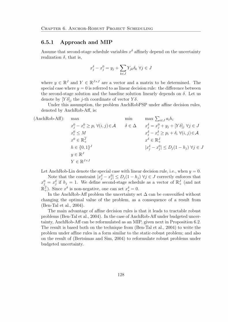
Chapter 6. Anchor-Robust Project Scheduling
6.5.1 Approach and MIP
Assume that second-stage schedule variables xδ affinely depend on the uncertaintyrealization δ, that is,
xδj − x0j = yj +
∑k∈J
Yjkδk ∀j ∈ J
where y ∈ RJ and Y ∈ RJ×J are a vector and a matrix to be determined. Thespecial case where y = 0 is referred to as linear decision rule: the difference betweenthe second-stage solution and the baseline solution linearly depends on δ. Let usdenote by [Y δ]j the j-th coordinate of vector Y δ.
Under this assumption, the problem AnchRobPSP under affine decision rules,denoted by AnchRob-Aff, is:
(AnchRob-Aff): max min max∑
i∈J aihi
x0j − x0
i ≥ pi ∀(i, j)∈A δ ∈ ∆ xδj = x0j + yj + [Y δ]j ∀j ∈ J
x0t ≤M xδj − xδi ≥ pi + δi ∀(i, j)∈Ax0 ∈ RJ
+ xδ ∈ RJ+
h ∈ {0, 1}J |xδj − x0j | ≤ Dj(1− hj) ∀j ∈ J
y ∈ RJ
Y ∈ RJ×J
Let AnchRob-Lin denote the special case with linear decision rule, i.e., when y = 0.Note that the constraint |xδj − x0
j | ≤ Dj(1− hj) ∀j ∈ J correctly enforces thatx0j = xδj if hj = 1. We define second-stage schedule as a vector of RJ
+ (and not
RJ+). Since xδ is non-negative, one can set xδs = 0.
In the AnchRob-Aff problem the uncertainty set ∆ can be convexified withoutchanging the optimal value of the problem, as a consequence of a result from(Ben-Tal et al., 2004).
The main advantage of affine decision rules is that it leads to tractable robustproblems (Ben-Tal et al., 2004). In the case of AnchRob-Aff under budgeted uncer-tainty, AnchRob-Aff can be reformulated as an MIP, given next in Proposition 6.2.The result is based both on the technique from (Ben-Tal et al., 2004) to write theproblem under affine rules in a form similar to the static-robust problem; and alsoon the result of (Bertsimas and Sim, 2004) to reformulate robust problems underbudgeted uncertainty.
128
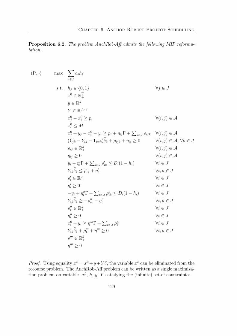
Chapter 6. Anchor-Robust Project Scheduling
Proposition 6.2. The problem AnchRob-Aff admits the following MIP reformu-lation.
(Paff) max∑i∈J
aihi
s.t. hj ∈ {0, 1} ∀j ∈ Jx0 ∈ RJ
+
y ∈ RJ
Y ∈ RJ×J
x0j − x0
i ≥ pi ∀(i, j) ∈ Ax0t ≤M
x0j + yj − x0
i − yi ≥ pi + ηijΓ +∑
k∈J ρijk ∀(i, j) ∈ A(Yjk − Yik − 1i=k)δk + ρijk + ηij ≥ 0 ∀(i, j) ∈ A, ∀k ∈ Jρij ∈ RJ
+ ∀(i, j) ∈ Aηij ≥ 0 ∀(i, j) ∈ Ayi + η′iΓ +
∑k∈J ρ
′ik ≤ Di(1− hi) ∀i ∈ J
Yikδk ≤ ρ′ik + η′i ∀i, k ∈ Jρ′i ∈ RJ
+ ∀i ∈ Jη′i ≥ 0 ∀i ∈ J−yi + η′′i Γ +
∑k∈J ρ
′′ik ≤ Di(1− hi) ∀i ∈ J
Yikδk ≥ −ρ′′ik − η′′i ∀i, k ∈ Jρ′′i ∈ RJ
+ ∀i ∈ Jη′′i ≥ 0 ∀i ∈ Jx0i + yi ≥ η′′′Γ +
∑k∈J ρ
′′′k ∀i ∈ J
Yikδk + ρ′′′k + η′′′ ≥ 0 ∀i, k ∈ Jρ′′′ ∈ RJ
+
η′′′ ≥ 0
Proof. Using equality xδ = x0 +y+Y δ, the variable xδ can be eliminated from therecourse problem. The AnchRob-Aff problem can be written as a single maximiza-tion problem on variables x0, h, y, Y satisfying the (infinite) set of constraints:
129
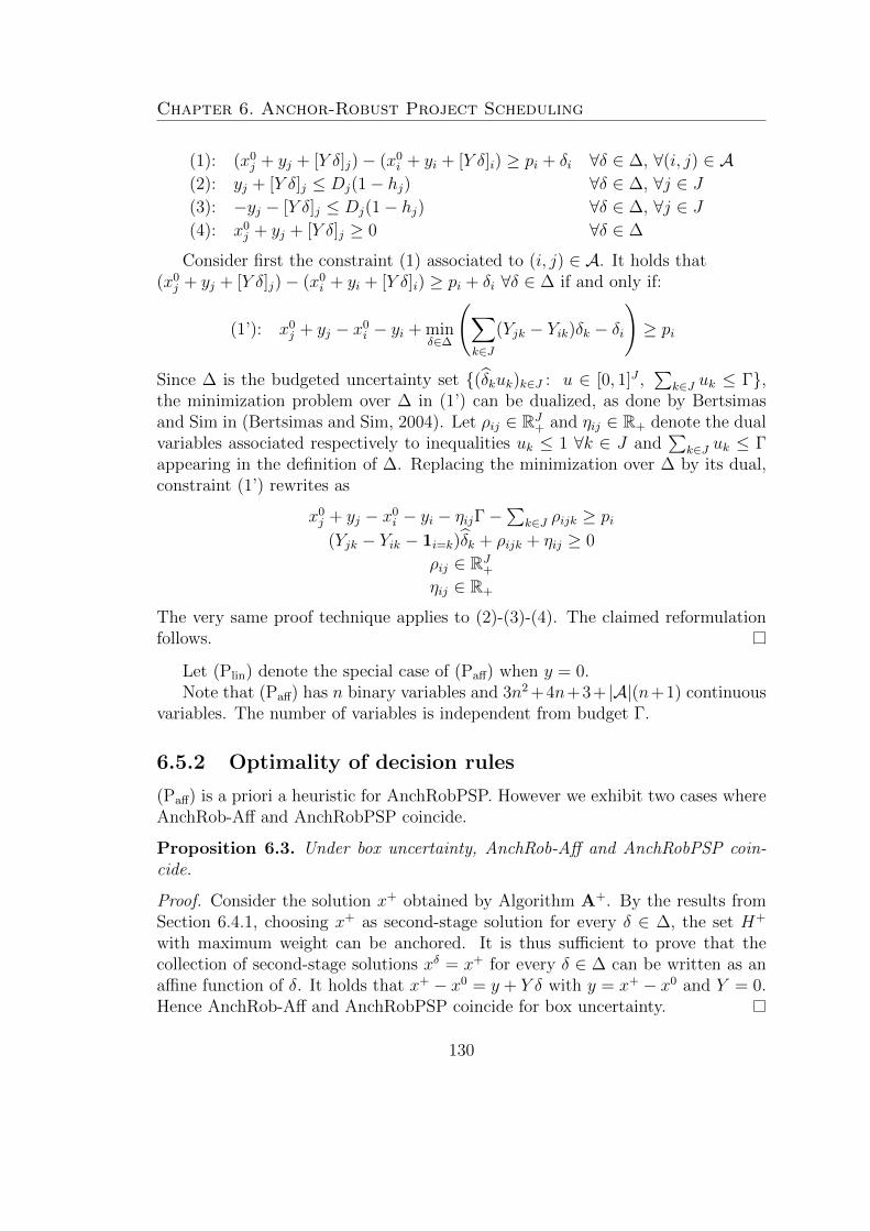
Chapter 6. Anchor-Robust Project Scheduling
(1): (x0j + yj + [Y δ]j)− (x0
i + yi + [Y δ]i) ≥ pi + δi ∀δ ∈ ∆, ∀(i, j) ∈ A(2): yj + [Y δ]j ≤ Dj(1− hj) ∀δ ∈ ∆, ∀j ∈ J(3): −yj − [Y δ]j ≤ Dj(1− hj) ∀δ ∈ ∆, ∀j ∈ J(4): x0
j + yj + [Y δ]j ≥ 0 ∀δ ∈ ∆
Consider first the constraint (1) associated to (i, j) ∈ A. It holds that(x0
j + yj + [Y δ]j)− (x0i + yi + [Y δ]i) ≥ pi + δi ∀δ ∈ ∆ if and only if:
(1’): x0j + yj − x0
i − yi + minδ∈∆
(∑k∈J
(Yjk − Yik)δk − δi
)≥ pi
Since ∆ is the budgeted uncertainty set {(δkuk)k∈J : u ∈ [0, 1]J ,∑
k∈J uk ≤ Γ},the minimization problem over ∆ in (1’) can be dualized, as done by Bertsimasand Sim in (Bertsimas and Sim, 2004). Let ρij ∈ RJ
+ and ηij ∈ R+ denote the dualvariables associated respectively to inequalities uk ≤ 1 ∀k ∈ J and
∑k∈J uk ≤ Γ
appearing in the definition of ∆. Replacing the minimization over ∆ by its dual,constraint (1’) rewrites as
x0j + yj − x0
i − yi − ηijΓ−∑
k∈J ρijk ≥ pi(Yjk − Yik − 1i=k)δk + ρijk + ηij ≥ 0
ρij ∈ RJ+
ηij ∈ R+
The very same proof technique applies to (2)-(3)-(4). The claimed reformulationfollows.
Let (Plin) denote the special case of (Paff) when y = 0.Note that (Paff) has n binary variables and 3n2 +4n+3+ |A|(n+1) continuous
variables. The number of variables is independent from budget Γ.
6.5.2 Optimality of decision rules
(Paff) is a priori a heuristic for AnchRobPSP. However we exhibit two cases whereAnchRob-Aff and AnchRobPSP coincide.
Proposition 6.3. Under box uncertainty, AnchRob-Aff and AnchRobPSP coin-cide.
Proof. Consider the solution x+ obtained by Algorithm A+. By the results fromSection 6.4.1, choosing x+ as second-stage solution for every δ ∈ ∆, the set H+
with maximum weight can be anchored. It is thus sufficient to prove that thecollection of second-stage solutions xδ = x+ for every δ ∈ ∆ can be written as anaffine function of δ. It holds that x+ − x0 = y + Y δ with y = x+ − x0 and Y = 0.Hence AnchRob-Aff and AnchRobPSP coincide for box uncertainty.
130
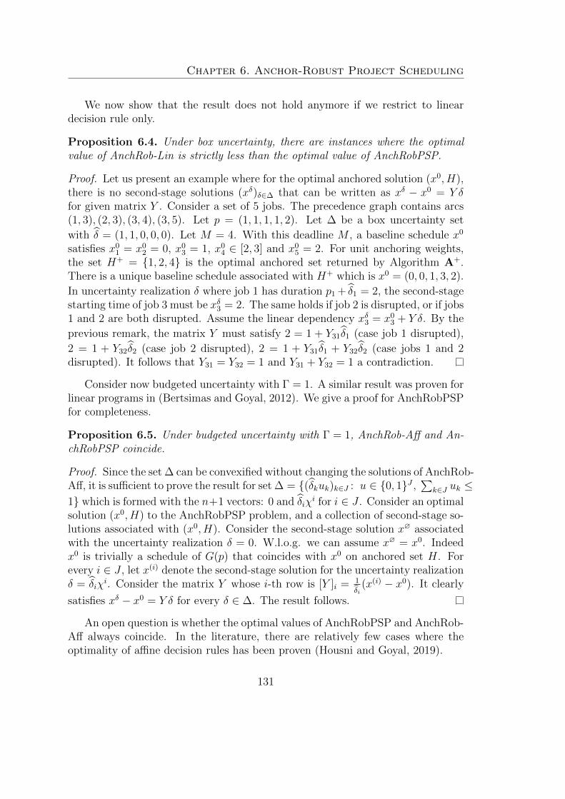
Chapter 6. Anchor-Robust Project Scheduling
We now show that the result does not hold anymore if we restrict to lineardecision rule only.
Proposition 6.4. Under box uncertainty, there are instances where the optimalvalue of AnchRob-Lin is strictly less than the optimal value of AnchRobPSP.
Proof. Let us present an example where for the optimal anchored solution (x0, H),there is no second-stage solutions (xδ)δ∈∆ that can be written as xδ − x0 = Y δfor given matrix Y . Consider a set of 5 jobs. The precedence graph contains arcs(1, 3), (2, 3), (3, 4), (3, 5). Let p = (1, 1, 1, 1, 2). Let ∆ be a box uncertainty set
with δ = (1, 1, 0, 0, 0). Let M = 4. With this deadline M , a baseline schedule x0
satisfies x01 = x0
2 = 0, x03 = 1, x0
4 ∈ [2, 3] and x05 = 2. For unit anchoring weights,
the set H+ = {1, 2, 4} is the optimal anchored set returned by Algorithm A+.There is a unique baseline schedule associated with H+ which is x0 = (0, 0, 1, 3, 2).
In uncertainty realization δ where job 1 has duration p1 + δ1 = 2, the second-stagestarting time of job 3 must be xδ3 = 2. The same holds if job 2 is disrupted, or if jobs1 and 2 are both disrupted. Assume the linear dependency xδ3 = x0
3 + Y δ. By the
previous remark, the matrix Y must satisfy 2 = 1 + Y31δ1 (case job 1 disrupted),
2 = 1 + Y32δ2 (case job 2 disrupted), 2 = 1 + Y31δ1 + Y32δ2 (case jobs 1 and 2disrupted). It follows that Y31 = Y32 = 1 and Y31 + Y32 = 1 a contradiction.
Consider now budgeted uncertainty with Γ = 1. A similar result was proven forlinear programs in (Bertsimas and Goyal, 2012). We give a proof for AnchRobPSPfor completeness.
Proposition 6.5. Under budgeted uncertainty with Γ = 1, AnchRob-Aff and An-chRobPSP coincide.
Proof. Since the set ∆ can be convexified without changing the solutions of AnchRob-Aff, it is sufficient to prove the result for set ∆ = {(δkuk)k∈J : u ∈ {0, 1}J ,
∑k∈J uk ≤
1} which is formed with the n+1 vectors: 0 and δiχi for i ∈ J . Consider an optimal
solution (x0, H) to the AnchRobPSP problem, and a collection of second-stage so-lutions associated with (x0, H). Consider the second-stage solution x∅ associatedwith the uncertainty realization δ = 0. W.l.o.g. we can assume x∅ = x0. Indeedx0 is trivially a schedule of G(p) that coincides with x0 on anchored set H. Forevery i ∈ J , let x(i) denote the second-stage solution for the uncertainty realizationδ = δiχ
i. Consider the matrix Y whose i-th row is [Y ]i = 1
δi(x(i) − x0). It clearly
satisfies xδ − x0 = Y δ for every δ ∈ ∆. The result follows.
An open question is whether the optimal values of AnchRobPSP and AnchRob-Aff always coincide. In the literature, there are relatively few cases where theoptimality of affine decision rules has been proven (Housni and Goyal, 2019).
131
Chapter 6. Anchor-Robust Project Scheduling
6.6 Numerical results
In this section, we highlight the relevance of AnchRobPSP under box or budgeteduncertainty, based on numerical experiments. We assess the numerical perfor-mances of the MIP formulation (Lay) from Section 6.2.2 and heuristic A+ fromSection 6.4.1. In particular we compare them to MIP reformulations under affineor linear decision rules. We study the impact of parameters (budget Γ, deadlineM) on solutions of the problem, and show that AnchRobPSP provides a convenientway to control the price of robustness.
6.6.1 General Settings
Instances. For evaluation purpose, different categories of instances are consid-ered, either randomly generated or taken from the literature. Let us first describethe precedence graphs of the instances.
• In PSP instances, the precedence graphs are taken from the PSPLib (Kolischand Sprecher, 1996), a benchmark for the Resource-Constrained ProjectScheduling Problem. We consider 50 instances from the families j120i, withi ∈ {1, . . . , 5}, which are the largest instances available (n = 120 jobs).• In ER instances, the precedence graphs are generated as follows. The num-
ber of jobs n ranges in {30, 60, 100, 200}. Precedence graphs are generatedrandomly with Erdos-Renyi (ER) model, i.e., between each pair of jobs i < jthe arc (i, j) is added with probability pr = 10
n. Processing times of jobs are
generated uniformly in {1, . . . , 20}.• In ERC instances, the precedence graphs are the same as ER instances,
but with modified processing times so that every job is on a Critical path.Processing times of jobs are increased by repeating the two following stepsuntil every job is on a critical path: (i) find a job i with positive marginm = LG(p)(s, t)− (LG(p)(s, i) + LG(p)(i, t)) > 0 (ii) increment pi of a randomvalue in {1, . . . ,m}.
For all instances, the uncertainty set ∆ is a budgeted uncertainty set for agiven budget Γ, and values δi drawn uniformly from [0, 0.5pi]. We considered50 PSP instances, and we generated 10 ER instances and 10 ERC instances foreach value of n ∈ {30, 60, 100, 200}, thus resulting in a total of 40 ER instancesand 40 ERC instances. Tests were performed with unit anchoring weights. Thedeadline M is chosen between the minimum makespan Mmin = LG(p)(s, t) and thesmallest deadline Mmax = LG∆[J ](s, t) for which all jobs can be anchored. Whenthe deadline M has to be fixed, it is defined arbitrarily as a convex combinationof Mmin and Mmax. Note that the value of Γ or M used in experiments will bespecified in the sequel when necessary.
132
Chapter 6. Anchor-Robust Project Scheduling
Since PSP instances correspond to a reference for another problem, they havelimited relevance for our purpose: namely, they feature precedence graphs withsmall degree. In constrast, in ER instances the expected value of the average degreein the precedence graph is driven by the constant n×pr, which we arbitrarily fixedat 10. Finally ERC instances are motivated by applications to industrial projects,where it can be observed that a lot of paths are critical or almost critical in thebaseline instance.
Implementation. Algorithms for AnchRobPSP were implemented with Julia0.6.2. MIP formulations were solved using JuMP v0.18.1 and Cplex 12.8. Note thatall considered MIP formulations, either (Lay) or (Paff), are compact. Numericalexperiments were completed on a PC with Intel Core i7-7500U CPU @ 2.70GHz2.90GHz and 8 Go RAM.
6.6.2 Performance of formulation (Lay) and A+ heuristic
Formulation (Lay). Let us first give numerical results of formulation (Lay)on the considered instances. We consider unit anchoring weights. In Table 6.1and Table 6.2 are reported for ER instances and ERC instances respectively, forn = 30, 60, 100, 200, 400, 600 and Γ = 1, 2, 3:– opt: the optimal value of the MIP reformulation;
– time: the computation time, in seconds;
– #nodes: the number of nodes explored by Cplex.
Note first that the number of anchored jobs is smaller for ERC instances thenfor ER instances, as a consequence from the design of ERC instances.
It can be seen that formulation (Lay) is efficient to solve instances up to 600jobs: the worst average computation time is 14.54 seconds for ER instances, n =600, Γ = 2. The number of nodes is small; in particular the problem is solved atroot node for all ERC instances with budget Γ ≥ 3. When the uncertainty budgetincreases, the size of formulation (Lay) is increased. However this does not lead toharder instances, e.g., the number of nodes for ER instances is smaller for Γ = 3than for Γ = 2, and all ERC instances are solved at root node. These results showthat formulation (Lay) is efficient to solve AnchRobPSP instances.
133
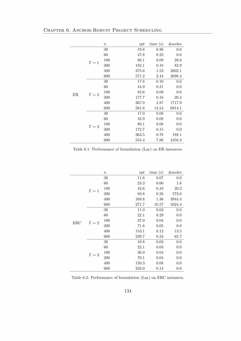
Chapter 6. Anchor-Robust Project Scheduling
n opt time (s) #nodes
ER
Γ = 1
30 19.8 0.36 0.0
60 47.8 0.22 0.0
100 86.1 0.09 28.8
200 182.1 0.18 82.9
400 375.6 1.53 2602.1
600 571.2 2.44 2698.4
Γ = 2
30 17.8 0.10 0.0
60 44.9 0.21 0.0
100 82.6 0.09 0.0
200 177.7 0.16 20.4
400 367.9 2.87 1717.9
600 561.6 14.54 6914.1
Γ = 3
30 17.0 0.08 0.0
60 42.9 0.08 0.0
100 80.1 0.08 0.0
200 172.7 0.15 0.0
400 363.5 0.78 188.1
600 554.4 7.86 2458.3
Table 6.1: Performance of formulation (Lay) on ER instances.
n opt time (s) #nodes
ERC
Γ = 1
30 11.6 0.07 0.0
60 23.3 0.06 1.6
100 42.6 0.10 20.2
200 83.8 0.28 573.8
400 169.8 1.36 3944.4
600 271.7 10.57 5024.4
Γ = 2
30 11.0 0.03 0.0
60 22.1 0.29 0.0
100 37.0 0.04 0.0
200 71.8 0.05 0.0
400 153.1 0.12 13.5
600 239.7 0.24 65.7
Γ = 3
30 10.8 0.02 0.0
60 22.1 0.03 0.0
100 36.0 0.04 0.0
200 70.1 0.04 0.0
400 150.3 0.08 0.0
600 233.0 0.14 0.0
Table 6.2: Performance of formulation (Lay) on ERC instances.
134
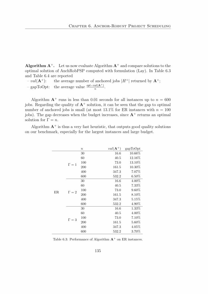
Chapter 6. Anchor-Robust Project Scheduling
Algorithm A+. Let us now evaluate Algorithm A+ and compare solutions to theoptimal solution of AnchRobPSP computed with formulation (Lay). In Table 6.3and Table 6.4 are reported– val(A+): the average number of anchored jobs |H+| returned by A+;
– gapToOpt: the average value opt−val(A+)n
.
Algorithm A+ runs in less than 0.01 seconds for all instances up to n = 600jobs. Regarding the quality of A+ solution, it can be seen that the gap to optimalnumber of anchored jobs is small (at most 13.1% for ER instances with n = 100jobs). The gap decreases when the budget increases, since A+ returns an optimalsolution for Γ = n.
Algorithm A+ is thus a very fast heuristic, that outputs good quality solutionson our benchmark, especially for the largest instances and large budget.
n val(A+) gapToOpt
ER
Γ = 1
30 16.6 10.66%
60 40.5 12.16%
100 73.0 13.10%
200 161.5 10.30%
400 347.3 7.07%
600 532.2 6.50%
Γ = 2
30 16.6 4.00%
60 40.5 7.33%
100 73.0 9.60%
200 161.5 8.10%
400 347.3 5.15%
600 532.2 4.90%
Γ = 3
30 16.6 1.33%
60 40.5 4.00%
100 73.0 7.10%
200 161.5 5.60%
400 347.3 4.05%
600 532.2 3.70%
Table 6.3: Performance of Algorithm A+ on ER instances.
135
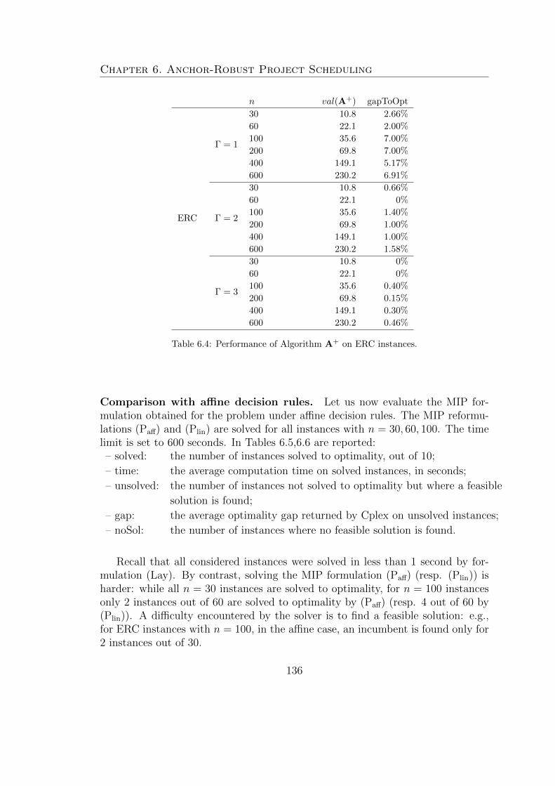
Chapter 6. Anchor-Robust Project Scheduling
n val(A+) gapToOpt
ERC
Γ = 1
30 10.8 2.66%
60 22.1 2.00%
100 35.6 7.00%
200 69.8 7.00%
400 149.1 5.17%
600 230.2 6.91%
Γ = 2
30 10.8 0.66%
60 22.1 0%
100 35.6 1.40%
200 69.8 1.00%
400 149.1 1.00%
600 230.2 1.58%
Γ = 3
30 10.8 0%
60 22.1 0%
100 35.6 0.40%
200 69.8 0.15%
400 149.1 0.30%
600 230.2 0.46%
Table 6.4: Performance of Algorithm A+ on ERC instances.
Comparison with affine decision rules. Let us now evaluate the MIP for-mulation obtained for the problem under affine decision rules. The MIP reformu-lations (Paff) and (Plin) are solved for all instances with n = 30, 60, 100. The timelimit is set to 600 seconds. In Tables 6.5,6.6 are reported:– solved: the number of instances solved to optimality, out of 10;
– time: the average computation time on solved instances, in seconds;
– unsolved: the number of instances not solved to optimality but where a feasible
solution is found;
– gap: the average optimality gap returned by Cplex on unsolved instances;
– noSol: the number of instances where no feasible solution is found.
Recall that all considered instances were solved in less than 1 second by for-mulation (Lay). By contrast, solving the MIP formulation (Paff) (resp. (Plin)) isharder: while all n = 30 instances are solved to optimality, for n = 100 instancesonly 2 instances out of 60 are solved to optimality by (Paff) (resp. 4 out of 60 by(Plin)). A difficulty encountered by the solver is to find a feasible solution: e.g.,for ERC instances with n = 100, in the affine case, an incumbent is found only for2 instances out of 30.
136
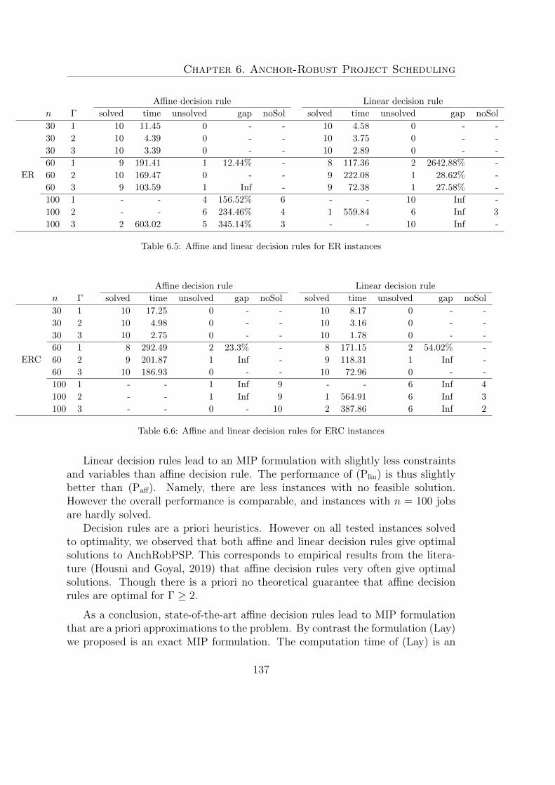
Chapter 6. Anchor-Robust Project Scheduling
Affine decision rule Linear decision rule
n Γ solved time unsolved gap noSol solved time unsolved gap noSol
ER
30 1 10 11.45 0 - - 10 4.58 0 - -
30 2 10 4.39 0 - - 10 3.75 0 - -
30 3 10 3.39 0 - - 10 2.89 0 - -
60 1 9 191.41 1 12.44% - 8 117.36 2 2642.88% -
60 2 10 169.47 0 - - 9 222.08 1 28.62% -
60 3 9 103.59 1 Inf - 9 72.38 1 27.58% -
100 1 - - 4 156.52% 6 - - 10 Inf -
100 2 - - 6 234.46% 4 1 559.84 6 Inf 3
100 3 2 603.02 5 345.14% 3 - - 10 Inf -
Table 6.5: Affine and linear decision rules for ER instances
Affine decision rule Linear decision rule
n Γ solved time unsolved gap noSol solved time unsolved gap noSol
ERC
30 1 10 17.25 0 - - 10 8.17 0 - -
30 2 10 4.98 0 - - 10 3.16 0 - -
30 3 10 2.75 0 - - 10 1.78 0 - -
60 1 8 292.49 2 23.3% - 8 171.15 2 54.02% -
60 2 9 201.87 1 Inf - 9 118.31 1 Inf -
60 3 10 186.93 0 - - 10 72.96 0 - -
100 1 - - 1 Inf 9 - - 6 Inf 4
100 2 - - 1 Inf 9 1 564.91 6 Inf 3
100 3 - - 0 - 10 2 387.86 6 Inf 2
Table 6.6: Affine and linear decision rules for ERC instances
Linear decision rules lead to an MIP formulation with slightly less constraintsand variables than affine decision rule. The performance of (Plin) is thus slightlybetter than (Paff). Namely, there are less instances with no feasible solution.However the overall performance is comparable, and instances with n = 100 jobsare hardly solved.
Decision rules are a priori heuristics. However on all tested instances solvedto optimality, we observed that both affine and linear decision rules give optimalsolutions to AnchRobPSP. This corresponds to empirical results from the litera-ture (Housni and Goyal, 2019) that affine decision rules very often give optimalsolutions. Though there is a priori no theoretical guarantee that affine decisionrules are optimal for Γ ≥ 2.
As a conclusion, state-of-the-art affine decision rules lead to MIP formulationthat are a priori approximations to the problem. By contrast the formulation (Lay)we proposed is an exact MIP formulation. The computation time of (Lay) is an
137
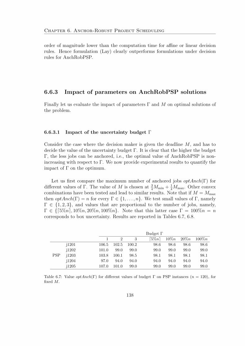
Chapter 6. Anchor-Robust Project Scheduling
order of magnitude lower than the computation time for affine or linear decisionrules. Hence formulation (Lay) clearly outperforms formulations under decisionrules for AnchRobPSP.
6.6.3 Impact of parameters on AnchRobPSP solutions
Finally let us evaluate the impact of parameters Γ and M on optimal solutions ofthe problem.
6.6.3.1 Impact of the uncertainty budget Γ
Consider the case where the decision maker is given the deadline M , and has todecide the value of the uncertainty budget Γ. It is clear that the higher the budgetΓ, the less jobs can be anchored, i.e., the optimal value of AnchRobPSP is non-increasing with respect to Γ. We now provide experimental results to quantify theimpact of Γ on the optimum.
Let us first compare the maximum number of anchored jobs optAnch(Γ) fordifferent values of Γ. The value of M is chosen at 3
4Mmin + 1
4Mmax. Other convex
combinations have been tested and lead to similar results. Note that if M = Mmax
then optAnch(Γ) = n for every Γ ∈ {1, . . . , n}. We test small values of Γ, namelyΓ ∈ {1, 2, 3}, and values that are proportional to the number of jobs, namely,Γ ∈ {d5%ne, 10%n, 20%n, 100%n}. Note that this latter case Γ = 100%n = ncorresponds to box uncertainty. Results are reported in Tables 6.7, 6.8.
Budget Γ
1 2 3 d5%ne 10%n 20%n 100%n
PSP
j1201 106.5 102.5 100.2 98.6 98.6 98.6 98.6
j1202 101.0 99.0 99.0 99.0 99.0 99.0 99.0
j1203 103.8 100.1 98.5 98.1 98.1 98.1 98.1
j1204 97.0 94.0 94.0 94.0 94.0 94.0 94.0
j1205 107.0 101.0 99.0 99.0 99.0 99.0 99.0
Table 6.7: Value optAnch(Γ) for different values of budget Γ on PSP instances (n = 120), forfixed M .
138
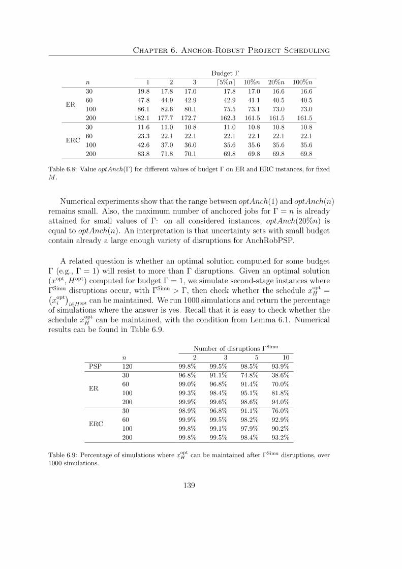
Chapter 6. Anchor-Robust Project Scheduling
Budget Γ
n 1 2 3 d5%ne 10%n 20%n 100%n
ER
30 19.8 17.8 17.0 17.8 17.0 16.6 16.6
60 47.8 44.9 42.9 42.9 41.1 40.5 40.5
100 86.1 82.6 80.1 75.5 73.1 73.0 73.0
200 182.1 177.7 172.7 162.3 161.5 161.5 161.5
ERC
30 11.6 11.0 10.8 11.0 10.8 10.8 10.8
60 23.3 22.1 22.1 22.1 22.1 22.1 22.1
100 42.6 37.0 36.0 35.6 35.6 35.6 35.6
200 83.8 71.8 70.1 69.8 69.8 69.8 69.8
Table 6.8: Value optAnch(Γ) for different values of budget Γ on ER and ERC instances, for fixedM .
Numerical experiments show that the range between optAnch(1) and optAnch(n)remains small. Also, the maximum number of anchored jobs for Γ = n is alreadyattained for small values of Γ: on all considered instances, optAnch(20%n) isequal to optAnch(n). An interpretation is that uncertainty sets with small budgetcontain already a large enough variety of disruptions for AnchRobPSP.
A related question is whether an optimal solution computed for some budgetΓ (e.g., Γ = 1) will resist to more than Γ disruptions. Given an optimal solution(xopt, Hopt) computed for budget Γ = 1, we simulate second-stage instances whereΓSimu disruptions occur, with ΓSimu > Γ, then check whether the schedule xopt
H =(xopti
)i∈Hopt can be maintained. We run 1000 simulations and return the percentage
of simulations where the answer is yes. Recall that it is easy to check whether theschedule xopt
H can be maintained, with the condition from Lemma 6.1. Numericalresults can be found in Table 6.9.
Number of disruptions ΓSimu
n 2 3 5 10
PSP 120 99.8% 99.5% 98.5% 93.9%
ER
30 96.8% 91.1% 74.8% 38.6%
60 99.0% 96.8% 91.4% 70.0%
100 99.3% 98.4% 95.1% 81.8%
200 99.9% 99.6% 98.6% 94.0%
ERC
30 98.9% 96.8% 91.1% 76.0%
60 99.9% 99.5% 98.2% 92.9%
100 99.8% 99.1% 97.9% 90.2%
200 99.8% 99.5% 98.4% 93.2%
Table 6.9: Percentage of simulations where xoptH can be maintained after ΓSimu disruptions, over
1000 simulations.
139
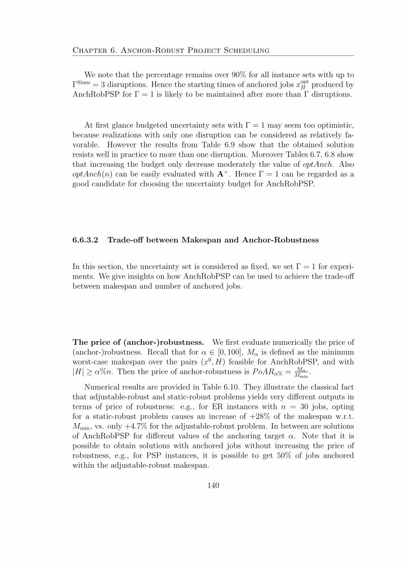
Chapter 6. Anchor-Robust Project Scheduling
We note that the percentage remains over 90% for all instance sets with up toΓSimu = 3 disruptions. Hence the starting times of anchored jobs xopt
H produced byAnchRobPSP for Γ = 1 is likely to be maintained after more than Γ disruptions.
At first glance budgeted uncertainty sets with Γ = 1 may seem too optimistic,because realizations with only one disruption can be considered as relatively fa-vorable. However the results from Table 6.9 show that the obtained solutionresists well in practice to more than one disruption. Moreover Tables 6.7, 6.8 showthat increasing the budget only decrease moderately the value of optAnch. AlsooptAnch(n) can be easily evaluated with A+. Hence Γ = 1 can be regarded as agood candidate for choosing the uncertainty budget for AnchRobPSP.
6.6.3.2 Trade-off between Makespan and Anchor-Robustness
In this section, the uncertainty set is considered as fixed, we set Γ = 1 for experi-ments. We give insights on how AnchRobPSP can be used to achieve the trade-offbetween makespan and number of anchored jobs.
The price of (anchor-)robustness. We first evaluate numerically the price of(anchor-)robustness. Recall that for α ∈ [0, 100], Mα is defined as the minimumworst-case makespan over the pairs (x0, H) feasible for AnchRobPSP, and with|H| ≥ α%n. Then the price of anchor-robustness is PoARα% = Mα
Mmin.
Numerical results are provided in Table 6.10. They illustrate the classical factthat adjustable-robust and static-robust problems yields very different outputs interms of price of robustness: e.g., for ER instances with n = 30 jobs, optingfor a static-robust problem causes an increase of +28% of the makespan w.r.t.Mmin, vs. only +4.7% for the adjustable-robust problem. In between are solutionsof AnchRobPSP for different values of the anchoring target α. Note that it ispossible to obtain solutions with anchored jobs without increasing the price ofrobustness, e.g., for PSP instances, it is possible to get 50% of jobs anchoredwithin the adjustable-robust makespan.
140
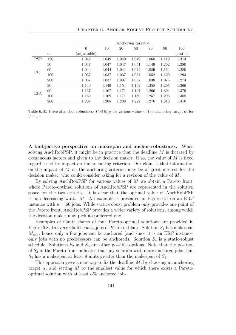
Chapter 6. Anchor-Robust Project Scheduling
Anchoring target α
0 10 20 50 80 90 100
n (adjustable) (static)
PSP 120 1.049 1.049 1.049 1.049 1.060 1.119 1.313
ER
30 1.047 1.047 1.047 1.051 1.149 1.202 1.280
60 1.044 1.044 1.044 1.044 1.089 1.164 1.280
100 1.037 1.037 1.037 1.037 1.052 1.129 1.293
200 1.037 1.037 1.037 1.037 1.038 1.076 1.274
ERC
30 1.149 1.149 1.154 1.192 1.258 1.295 1.366
60 1.167 1.167 1.171 1.197 1.266 1.304 1.379
100 1.169 1.169 1.171 1.189 1.257 1.296 1.388
200 1.208 1.208 1.208 1.222 1.276 1.313 1.410
Table 6.10: Price of anchor-robustness PoARα% for various values of the anchoring target α, forΓ = 1.
A biobjective perspective on makespan and anchor-robustness. Whensolving AnchRobPSP, it might be in practice that the deadline M is dictated byexogeneous factors and given to the decision maker. If so, the value of M is fixedregardless of its impact on the anchoring criterion. Our claim is that informationon the impact of M on the anchoring criterion may be of great interest for thedecision maker, who could consider asking for a revision of the value of M .
By solving AnchRobPSP for various values of M we obtain a Pareto front,where Pareto-optimal solutions of AnchRobPSP are represented in the solutionspace for the two criteria. It is clear that the optimal value of AnchRobPSPis non-decreasing w.r.t. M . An example is presented in Figure 6.7 on an ERCinstance with n = 60 jobs. While static-robust problem only provides one point ofthe Pareto front, AnchRobPSP provides a wider variety of solutions, among whichthe decision maker may pick its preferred one.
Examples of Gantt charts of four Pareto-optimal solutions are provided inFigure 6.8. In every Gantt chart, jobs of H are in black. Solution S1 has makespanMmin, hence only a few jobs can be anchored (and since it is an ERC instance,only jobs with no predecessors can be anchored). Solution S4 is a static-robustschedule. Solutions S2 and S3 are other possible options. Note that the positionof S3 in the Pareto front indicates that any solution with more anchored jobs thanS3 has a makespan at least 9 units greater than the makespan of S3.
This approach gives a new way to fix the deadline M , by choosing an anchoringtarget α, and setting M to the smallest value for which there exists a Pareto-optimal solution with at least α% anchored jobs.
141
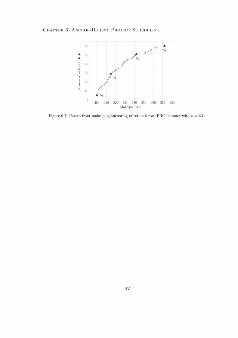
Chapter 6. Anchor-Robust Project Scheduling
300 310 320 330 340 350 360 370 3800
10
20
30
40
50
60
S1
S2
S3
S4
Makespan of x
Num
ber
ofan
chor
edjo
b|H|
Figure 6.7: Pareto front makespan/anchoring criterion for an ERC instance with n = 60.
142
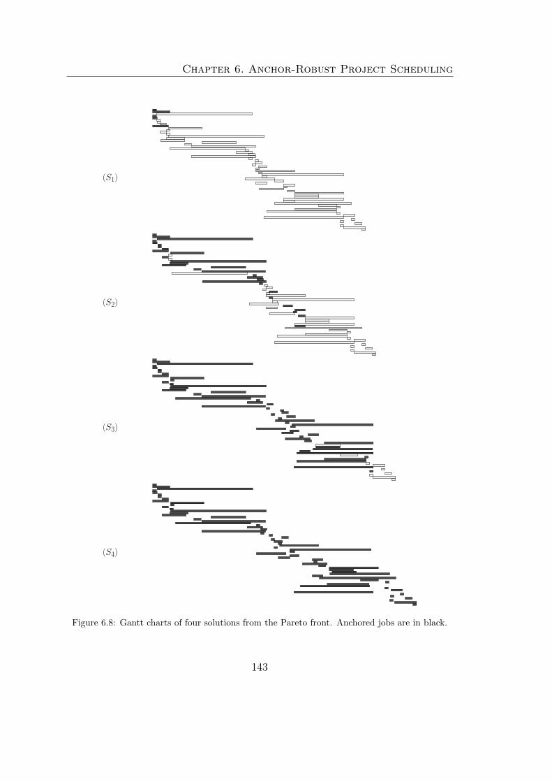
Chapter 6. Anchor-Robust Project Scheduling
(S1)
(S2)
(S3)
(S4)
Figure 6.8: Gantt charts of four solutions from the Pareto front. Anchored jobs are in black.
143
Chapter 6. Anchor-Robust Project Scheduling
Conclusion
Anchor-robustness was proposed as a concept standing between static-robust andadjustable-robust approaches, to achieve a trade-off between guarantee on startingtimes and cost of a solution, here corresponding to the schedule makespan. It ledto the definition of the AnchRobPSP problem.
In the present work we studied the structure of AnchRobPSP by exploiting boththe structure of the underlying project scheduling problem, and the properties ofbox or budgeted uncertainty. Based on these structural properties, we analyzed thecomputational complexity of the problem. AnchRobPSP was proven NP-hard forbudgeted uncertainty, while the corresponding adjustable-robust problem is solv-able in polynomial time. This increase in complexity stems from the binary natureof deciding whether a job is anchored or not, under the constraints imposed by theuncertainty set and the deadline. We then designed a compact MIP reformulationand algorithms. We emphasize that the proposed algorithmic tools, such as thelayered graph, are dedicated to the problem. The associated formulation (Lay)appears to outperform state-of-the-art generic techniques, such as decision rules.These results are good promises for the implementability of anchor-robustness asa concept, through efficient algoritmic approaches for AnchRobPSP.
In the line of the complexity analysis of AnchRobPSP, an open question is thecomplexity of the variant where the values L∆
ij are part of the input (or computablein polynomial time) and with unit anchoring weights. Another perspective is tofurther investigate mixed-integer programming techniques for the problem. Thisis done in Part IV of the thesis, where new MIP formulations for AnchRobPSPare proposed.
144
Chapter 7
The Anchor-Robust RCPSP:exact and heuristic approaches
In this chapter, we study anchor-robustness for the Resource-Constrained ProjectScheduling Problem (RCPSP). The RCPSP is to find a minimum makespan sched-ule for the jobs of a project under precedence constraints and scarce resource avail-ability. By contrast with PERT Scheduling, the RCPSP is a classical problemthat is NP-hard and computationally challenging to solve in practice (see, e.g.,(Artigues et al., 2008) for a survey). The RCPSP is ubiquitous in applications,where it often appears with uncertain parameters as it can be expected from anyreal-life problem. We focus on uncertainty in the processing times of the jobsand propose an anchor-robust optimization approach, in the spirit of the generalconcepts exposed in Chapter 2.
As pointed out in (Hazır and Ulusoy, 2020), research on robust optimizationfor the RCPSP is rather scarce, compared to stochastic project scheduling. In(Artigues et al., 2013) the authors studied a robust problem under a min regretcriterion. In (Bruni et al., 2017) the authors introduced the Adjustable-RobustRCPSP, derived from the general concept of adjustable robustness from (Ben-Talet al., 2004). Sequencing decisions (corresponding to resource allocation decisions)are fixed before uncertainty is known; by contrast the starting times of jobs adjustto the uncertainty realization. The goal is to minimize the worst-case makespan.As noted already in Chapter 6, adjustable-robustness outputs a worst-case make-span, but it gives no schedule to decide in advance since starting times depend onthe uncertainty realization. However, finding a precomputed baseline schedule isoften required in applications to prepare the implementation of the schedule. Thismotivates the study of an approach to compute a baseline solution with boundedmakespan, along with a subset of anchored decisions.
The main contributions of this chapter, corresponding to (Pass-Lanneau et al.,
145
Chapter 7. The Anchor-Robust RCPSP
2020), are the following. Anchored solutions are defined as a new concept in two-stage robust optimization for the RCPSP. The Anchor-Robust RCPSP is defined,to find a baseline schedule with bounded makespan, sequencing decisions, anda maximum number of anchored jobs. The connection with Adjustable-RobustRCPSP is pointed out. We show that these two problems can benefit from eachother, in order to find both a worst-case makespan and a baseline schedule. Weextend algorithmic tools from Chapter 6 and obtain a graph model and compactMIP reformulations for adjustable-robustness and anchor-robustness in a unifiedway. Heuristic algorithms are also proposed based on the same graph model. Weinvestigate numerical performance of the proposed compact reformulation for theAdjustable-Robust RCPSP on instances based on the PSPLib. We point out thatthe overhead computational effort for solving the Adjustable-Robust RCPSP, incomparison with the deterministic RCPSP, is low. We follow on by investigat-ing the efficiency of the proposed heuristic approaches to solve larger instances.We then provide numerical results for the Anchor-Robust RCPSP, for both MIPreformulation and heuristics. We highlight the good properties of anchor-robustsolutions for finding a trade-off between makespan and guarantee of starting times.
7.1 Preliminaries
Consider an instance of the RCPSP I = ((J,A, p), (rik)i∈J,k∈R, (Rk)k∈R). It isformed with a precedence graph (J,A, p), with p ∈ RJ
+ the processing times of jobs,and resource requirements (rik)i∈J,k∈R and resource capacity (Rk)k∈R). Given in-
stance I, the RCPSP is to find a schedule x ∈ RJ+ satisfying precedence constraints
of (J,A, p) and resource constraints, so that the makespan xt is minimized.
Consider processing times uncertainty. Processing times have nominal valuesp ∈ RJ
+ and their real value may be some p + δ, where deviation δ is assumedto be lying in uncertainty set ∆ ⊆ RJ
+. In this chapter we consider budgeted
uncertainty. The budgeted uncertainty set associated with vector δ ∈ RJ+ and
integer Γ is ∆ = {δ = (δiui)i∈J : u ∈ {0, 1}J ,∑
i∈J ui ≤ Γ}. If Γ = 0, set ∆ isreduced to the singleton {0}, and robust approaches reduce to the deterministicRCPSP. Note that ∆ is defined as a discrete set, and not a polytope; a result from(Ben-Tal et al., 2004) applicable to all robust approaches we consider, is that ∆can be convexified without changing the solutions. If Γ = |J |, the convex hull of
set ∆ is the box uncertainty set Πi∈J [0, δi], also known as interval uncertainty set.
Let I = ((J,A, p), (rik), (Rk)) denote the nominal RCPSP instance. Let alsoIδ = ((J,A, p+δ), (rik), (Rk)) be the instance where processing times are affectedby deviation δ ∈ ∆. A first attempt to account for uncertainty is to define theStatic-Robust RCPSP: given nominal instance I and set ∆, the problem is to find
146
Chapter 7. The Anchor-Robust RCPSP
a schedule x+ that is feasible for Iδ for every δ ∈ ∆, so as to minimize makespanx+t . The static-robust schedule x+ is likely to have a very large makespan. Note
in this case that changing the budget Γ has no impact on the price of robustness,as formalized in the following observation.
Observation 7.1. For every budget Γ ∈ {1, . . . , |J |}, solutions of the Static-
Robust RCPSP for budgeted uncertainty set ∆ = {(δiui)i∈J : u ∈ {0, 1}J ,∑
i∈J ui ≤Γ} are the same as solutions of the Static-Robust RCPSP for box uncertainty set
Πi∈J [0, δi].
Proof. Let Γ < |J |. Clearly a static-robust solution for box uncertainty is also
static-robust for ∆ since ∆ ⊆ Πi∈J [0, δi]. Conversely, assume that x is feasible foruncertainty set ∆. Let (i, j) ∈ A. It holds that xj − xi ≥ pi + δi for every δ ∈ ∆.
In particular for every budget Γ ≥ 1, the uncertainty realization where δi = δi isin ∆. Hence xj − xi ≥ pi + δi, and x is a schedule of (J,A, p + δ). Since δ is anupper-bound on the box uncertainty set, schedule x is a static-robust solution forbox uncertainty.
We mention that this result is not specific to the RCPSP problem, but from theuncertainty being on the right-hand side of constraints. This observation motivatesthe study of 2-stage robust approaches, where the schedule could be adapted touncertainty realization.
7.2 Anchor-Robust approach for the RCPSP
In this section we propose the concept of anchor-robustness for the RCPSP, basedon the general concepts of Chapter 2. We first recall the flow formulation forthe RCPSP, which serves as a basis for the proposed anchor-robust approach.Anchored sets are then formally defined, along with the Anchor-Robust RCPSP.Finally we highlight the connection with the Adjustable-Robust RCPSP from theliterature.
7.2.1 Flow formulation for the RCPSP
Let us first present the flow formulation for the RCPSP from the literature (Ar-tigues et al., 2003). Let J2 = {(i, j), i, j ∈ J, i 6= j}. With a schedule x satisfyingresource constraints, one can associate a so-called resource flow f . The resourceflow is a collection (fk)k∈R of s−t flows in the graph (J, J2). Flow fk has value Rk,and the quantity flowing through every job i ∈ J equals the resource requirement
147
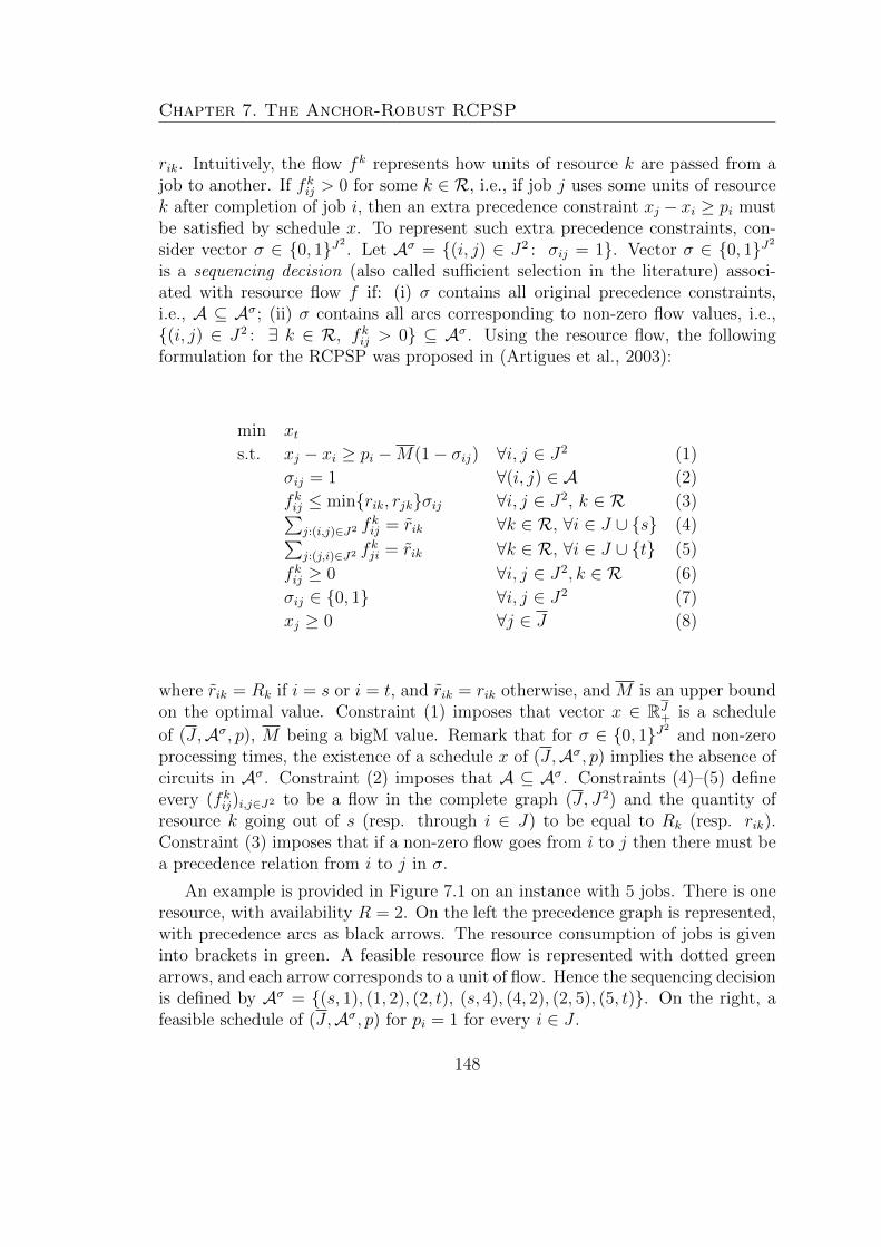
Chapter 7. The Anchor-Robust RCPSP
rik. Intuitively, the flow fk represents how units of resource k are passed from ajob to another. If fkij > 0 for some k ∈ R, i.e., if job j uses some units of resourcek after completion of job i, then an extra precedence constraint xj − xi ≥ pi mustbe satisfied by schedule x. To represent such extra precedence constraints, con-sider vector σ ∈ {0, 1}J2
. Let Aσ = {(i, j) ∈ J2 : σij = 1}. Vector σ ∈ {0, 1}J2
is a sequencing decision (also called sufficient selection in the literature) associ-ated with resource flow f if: (i) σ contains all original precedence constraints,i.e., A ⊆ Aσ; (ii) σ contains all arcs corresponding to non-zero flow values, i.e.,{(i, j) ∈ J2 : ∃ k ∈ R, fkij > 0} ⊆ Aσ. Using the resource flow, the followingformulation for the RCPSP was proposed in (Artigues et al., 2003):
min xts.t. xj − xi ≥ pi −M(1− σij) ∀i, j ∈ J2 (1)
σij = 1 ∀(i, j) ∈ A (2)
fkij ≤ min{rik, rjk}σij ∀i, j ∈ J2, k ∈ R (3)∑j:(i,j)∈J2 fkij = rik ∀k ∈ R, ∀i ∈ J ∪ {s} (4)∑j:(j,i)∈J2 fkji = rik ∀k ∈ R, ∀i ∈ J ∪ {t} (5)
fkij ≥ 0 ∀i, j ∈ J2, k ∈ R (6)
σij ∈ {0, 1} ∀i, j ∈ J2 (7)
xj ≥ 0 ∀j ∈ J (8)
where rik = Rk if i = s or i = t, and rik = rik otherwise, and M is an upper boundon the optimal value. Constraint (1) imposes that vector x ∈ RJ
+ is a schedule
of (J,Aσ, p), M being a bigM value. Remark that for σ ∈ {0, 1}J2and non-zero
processing times, the existence of a schedule x of (J,Aσ, p) implies the absence ofcircuits in Aσ. Constraint (2) imposes that A ⊆ Aσ. Constraints (4)–(5) defineevery (fkij)i,j∈J2 to be a flow in the complete graph (J, J2) and the quantity ofresource k going out of s (resp. through i ∈ J) to be equal to Rk (resp. rik).Constraint (3) imposes that if a non-zero flow goes from i to j then there must bea precedence relation from i to j in σ.
An example is provided in Figure 7.1 on an instance with 5 jobs. There is oneresource, with availability R = 2. On the left the precedence graph is represented,with precedence arcs as black arrows. The resource consumption of jobs is giveninto brackets in green. A feasible resource flow is represented with dotted greenarrows, and each arrow corresponds to a unit of flow. Hence the sequencing decisionis defined by Aσ = {(s, 1), (1, 2), (2, t), (s, 4), (4, 2), (2, 5), (5, t)}. On the right, afeasible schedule of (J,Aσ, p) for pi = 1 for every i ∈ J .
148
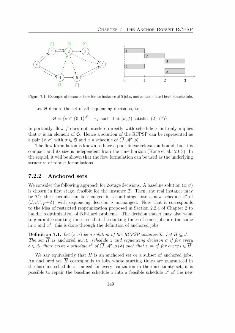
Chapter 7. The Anchor-Robust RCPSP
s
1 2 3
4 5
t
[1] [2] [0]
[1] [1]
12
34
5
0 1 2 3
Figure 7.1: Example of resource flow for an instance of 5 jobs, and an associated feasible schedule.
Let S denote the set of all sequencing decisions, i.e.,
S = {σ ∈ {0, 1}J2
: ∃f such that (σ, f) satisfies (2)–(7)}.
Importantly, flow f does not interfere directly with schedule x but only impliesthat σ is an element of S. Hence a solution of the RCPSP can be represented asa pair (x, σ) with σ ∈ S and x a schedule of (J,Aσ, p).
The flow formulation is known to have a poor linear relaxation bound, but it iscompact and its size is independent from the time horizon (Kone et al., 2013). Inthe sequel, it will be shown that the flow formulation can be used as the underlyingstructure of robust formulations.
7.2.2 Anchored sets
We consider the following approach for 2-stage decisions. A baseline solution (x, σ)is chosen in first stage, feasible for the instance I. Then, the real instance maybe Iδ: the schedule can be changed in second stage into a new schedule xδ of(J,Aσ, p+δ), with sequencing decision σ unchanged. Note that it correspondsto the idea of restricted reoptimization proposed in Section 2.2.4 of Chapter 2 tohandle reoptimization of NP-hard problems. The decision maker may also wantto guarantee starting times, so that the starting times of some jobs are the samein x and xδ: this is done through the definition of anchored jobs.
Definition 7.1. Let (z, σ) be a solution of the RCPSP instance I. Let H ⊆ J .The set H is anchored w.r.t. schedule z and sequencing decision σ if for everyδ ∈ ∆, there exists a schedule zδ of (J,Aσ, p+δ) such that zi = zδi for every i ∈ H.
We say equivalently that H is an anchored set or a subset of anchored jobs.An anchored set H corresponds to jobs whose starting times are guaranteed inthe baseline schedule z: indeed for every realization in the uncertainty set, it ispossible to repair the baseline schedule z into a feasible schedule zδ of the new
149
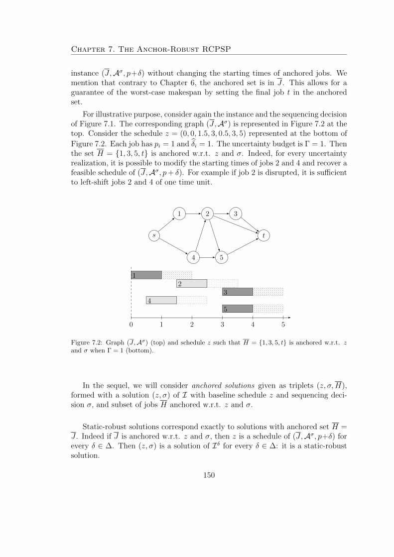
Chapter 7. The Anchor-Robust RCPSP
instance (J,Aσ, p+δ) without changing the starting times of anchored jobs. Wemention that contrary to Chapter 6, the anchored set is in J . This allows for aguarantee of the worst-case makespan by setting the final job t in the anchoredset.
For illustrative purpose, consider again the instance and the sequencing decisionof Figure 7.1. The corresponding graph (J,Aσ) is represented in Figure 7.2 at thetop. Consider the schedule z = (0, 0, 1.5, 3, 0.5, 3, 5) represented at the bottom of
Figure 7.2. Each job has pi = 1 and δi = 1. The uncertainty budget is Γ = 1. Thenthe set H = {1, 3, 5, t} is anchored w.r.t. z and σ. Indeed, for every uncertaintyrealization, it is possible to modify the starting times of jobs 2 and 4 and recover afeasible schedule of (J,Aσ, p+ δ). For example if job 2 is disrupted, it is sufficientto left-shift jobs 2 and 4 of one time unit.
s
1 2 3
4 5
t
1
3
5
2
4
0 1 2 3 4 5
Figure 7.2: Graph (J,Aσ) (top) and schedule z such that H = {1, 3, 5, t} is anchored w.r.t. zand σ when Γ = 1 (bottom).
In the sequel, we will consider anchored solutions given as triplets (z, σ,H),formed with a solution (z, σ) of I with baseline schedule z and sequencing deci-sion σ, and subset of jobs H anchored w.r.t. z and σ.
Static-robust solutions correspond exactly to solutions with anchored set H =J . Indeed if J is anchored w.r.t. z and σ, then z is a schedule of (J,Aσ, p+δ) forevery δ ∈ ∆. Then (z, σ) is a solution of Iδ for every δ ∈ ∆: it is a static-robustsolution.
150
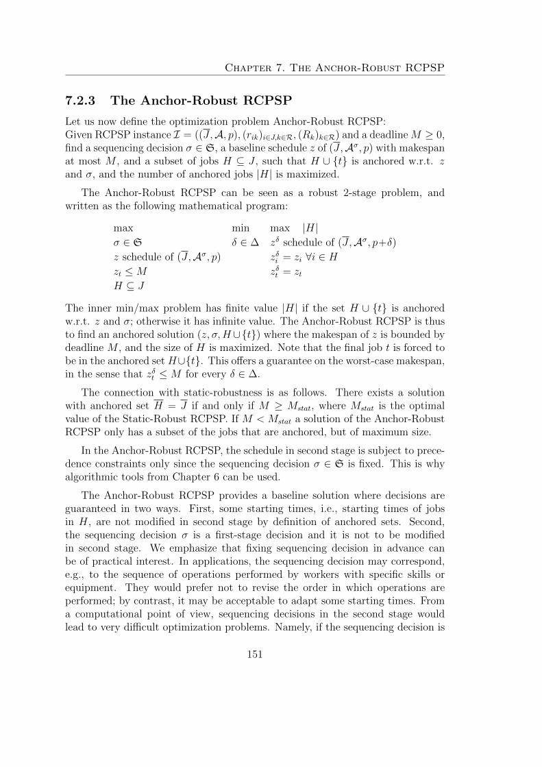
Chapter 7. The Anchor-Robust RCPSP
7.2.3 The Anchor-Robust RCPSP
Let us now define the optimization problem Anchor-Robust RCPSP:Given RCPSP instance I = ((J,A, p), (rik)i∈J,k∈R, (Rk)k∈R) and a deadline M ≥ 0,find a sequencing decision σ ∈ S, a baseline schedule z of (J,Aσ, p) with makespanat most M , and a subset of jobs H ⊆ J , such that H ∪ {t} is anchored w.r.t. zand σ, and the number of anchored jobs |H| is maximized.
The Anchor-Robust RCPSP can be seen as a robust 2-stage problem, andwritten as the following mathematical program:
max min max |H|σ ∈ S δ ∈ ∆ zδ schedule of (J,Aσ, p+δ)
z schedule of (J,Aσ, p) zδi = zi ∀i ∈ Hzt ≤M zδt = ztH ⊆ J
The inner min/max problem has finite value |H| if the set H ∪ {t} is anchoredw.r.t. z and σ; otherwise it has infinite value. The Anchor-Robust RCPSP is thusto find an anchored solution (z, σ,H∪{t}) where the makespan of z is bounded bydeadline M , and the size of H is maximized. Note that the final job t is forced tobe in the anchored set H∪{t}. This offers a guarantee on the worst-case makespan,in the sense that zδt ≤M for every δ ∈ ∆.
The connection with static-robustness is as follows. There exists a solutionwith anchored set H = J if and only if M ≥ Mstat, where Mstat is the optimalvalue of the Static-Robust RCPSP. If M < Mstat a solution of the Anchor-RobustRCPSP only has a subset of the jobs that are anchored, but of maximum size.
In the Anchor-Robust RCPSP, the schedule in second stage is subject to prece-dence constraints only since the sequencing decision σ ∈ S is fixed. This is whyalgorithmic tools from Chapter 6 can be used.
The Anchor-Robust RCPSP provides a baseline solution where decisions areguaranteed in two ways. First, some starting times, i.e., starting times of jobsin H, are not modified in second stage by definition of anchored sets. Second,the sequencing decision σ is a first-stage decision and it is not to be modifiedin second stage. We emphasize that fixing sequencing decision in advance canbe of practical interest. In applications, the sequencing decision may correspond,e.g., to the sequence of operations performed by workers with specific skills orequipment. They would prefer not to revise the order in which operations areperformed; by contrast, it may be acceptable to adapt some starting times. Froma computational point of view, sequencing decisions in the second stage wouldlead to very difficult optimization problems. Namely, if the sequencing decision is
151
Chapter 7. The Anchor-Robust RCPSP
in second stage, even deciding if the starting time of a job can be guaranteed, isNP-hard. This corresponds to the NP-hardness results obtained in Chapter 5.
7.2.4 Connection with the Adjustable-Robust RCPSP
An adjustable-robust approach for the RCPSP was proposed in (Bruni et al., 2017).First stage decision is the sequencing decision σ ∈ S; schedule x is decided insecond stage. The Adjustable-Robust RCPSP writes as the following mathematicalprogram:
min max min xδtσ ∈ S δ ∈ ∆ s.t. xδ schedule of (J,Aσ, p+δ)
Let QΓ(σ) denote the inner max-min problem, i.e., the worst-case makespan forsequencing decision σ ∈ S. The Adjustable-Robust RCPSP is then to minimizeQΓ(σ) for σ ∈ S.
Contrary to the anchor-robust approach, the Adjustable-Robust RCPSP doesnot include the computation of a baseline schedule. However the Adjustable-Robust RCPSP is related to anchored sets by the following observation.
Observation 7.2. Let σ ∈ S. The worst-case makespan QΓ(σ) is equal to theminimum makespan of z, where (z, σ, {t}) is an anchored solution.
Proof. By definition QΓ(σ) is the minimum value M such that for every δ ∈ ∆,there exists a schedule xδ of (J,Aσ, p+δ) with makespan at most M . Equivalently,it is the minimum M such that z is a schedule of (J,Aσ, p) with zt = M , and {t}is anchored w.r.t. z and σ, by definition of anchored solutions.
A consequence of Observation 7.2 is that there exists a solution of the Anchor-Robust RCPSP if and only if M ≥ Madj, where Madj is the optimal value ofthe Adjustable-Robust RCPSP. The singleton {t} can be anchored if and only ifM ≥ Madj. Note that even with deadline M = Madj, there exists solutions withanchored set H∪{t}, H 6= ∅, as illustrated in Section 7.6. That is, it is possible toguarantee a non-trivial subset of starting times without increasing the worst-casemakespan Madj.
The Adjustable-Robust RCPSP and the Anchor-Robust RCPSP can benefitfrom each other in the following way. First the Adjustable-Robust RCPSP can besolved to determine a robust worst-case makespan Madj. Then the Anchor-RobustRCPSP can be solved with deadline Madj to determine schedule z∗ satisfying thisdeadline, sequencing decision σ∗, along with an anchored set H∗.
152
Chapter 7. The Anchor-Robust RCPSP
Let us review the approaches proposed in the literature to solve the Adjustable-Robust RCPSP. In (Bruni et al., 2017) the problem was introduced and a Bendersdecomposition was proposed. The computation of QΓ(σ) for fixed σ appears assubproblem. The authors then focused on budgeted uncertainty and proved thatQΓ(σ) can be computed in polynomial time by dynamic programming in thatcase. Note that it is the same problem solved in (Minoux, 2007a). The authorsproposed enhancements to the Benders decomposition algorithm, evaluated oninstances built upon the PSPLib. In (Bruni et al., 2018) the same authors inves-tigated two new methods: a primal and a dual one. The dual method has thesame subproblem as in (Bruni et al., 2017) but other cuts associated with dualinformation are added on the fly. The primal method is a column-and-constraintgeneration scheme inspired from (Zeng and Zhao, 2013). Computational compar-ison of the two decomposition approaches of (Bruni et al., 2018) and the one of(Bruni et al., 2017) is reported. In (Bold and Goerigk, 2020) a compact refor-mulation for the Adjustable-Robust RCPSP is proposed, independently from thepresent work.
7.3 Graph model and compact MIP
reformulations
In this section, we extend the layered graph from Chapter 6 to characterize an-chored sets and solutions of the Anchor-Robust RCPSP. Compact MIP reformula-tions are deduced for the Anchor-Robust RCPSP and for the Adjustable-RobustRCPSP. Heuristics based on the graph model are also proposed.
7.3.1 Layered graph
Let us propose a graph model based on the layered graph. Let ∆ be the bud-geted uncertainty set defined by deviation δ ∈ RJ
+ and budget Γ, and let nominalprocessing times be p ∈ RJ
+.
Let (J,A, p) be a precedence graph. For H ⊆ J , consider the layered graphGlay(A, H). There is no difference with the definition of Chapter 6, except thatthere are additional vertical arcs between copies of t if t ∈ H. Let us recall theconstruction of Glay(A, H). It contains Γ + 1 layers, indexed from 0 to Γ. Eachlayer γ contains a copy of the set of jobs, denoted by iγ, i ∈ J . The arc-set ofthe layered graph contains three types of arcs. Horizontal arcs are arcs (iγ, jγ) forevery γ and (i, j) ∈ A, with arc-weights pi. Transversal arcs are arcs (iγ+1, jγ) for
153
Chapter 7. The Anchor-Robust RCPSP
every γ < Γ and (i, j) ∈ A, with arc-weights pi + δi. Vertical arcs are arcs (jγ, jΓ)for every j ∈ H, γ < Γ, with arc-weights 0.
Note that the layered graph has all information from ∆, since the number oflayers depends on the uncertainty budget Γ, and deviations δ appear on arc-weightsof transversal arcs. Note also that if the graph (J,A) is acyclic, then Glay(A, H)is acyclic. In Chapter 6 the set H was defined as a subset of J and not J , but allresults extend to the case of a set H containing s or t.
Let us now derive a characterization of anchored sets for the RCPSP. It followsdirectly from Definition 7.1 and Theorem 6.2 that
Theorem 7.1. Let (z, σ) be a solution of the RCPSP instance I. Let H ⊆ J .The set H is anchored w.r.t. sequencing decision σ and schedule z if and only ifthere exists x a schedule of Glay(Aσ, H) such that xΓ
i = zi for every i ∈ J .
Combining Observation 7.2 and Theorem 7.1, it follows that
Corollary 7.1. For every σ ∈ S, the worst-case makespan QΓ(σ) is equal to theminimum value of xΓ
t for x a schedule of Glay(Aσ, {t}).
Hence the layered graph can be used to compute the worst-case makespanQΓ(σ), since the minimum value of xΓ
t for x a schedule of Glay(Aσ, {t}) is equal tothe length of the longest sΓ−tΓ path in Glay(Aσ, {t}). Recall that Glay(Aσ, {t}) isacyclic when (J,Aσ) is acyclic. Such longest path can be computed in polynomialtime by dynamic programming.
7.3.2 Compact MIP reformulations
Let us now introduce new MIP reformulation for the Anchor-Robust and Adjustable-Robust RCPSP. The formulations involve the following decision variables:– variables f and σ as in the flow formulation for the RCPSP;– continuous variables xγj ≥ 0 for every j ∈ J , γ ∈ {0, . . . ,Γ};– for the Anchor-Robust RCPSP, binary variables h ∈ {0, 1}J .
Theorem 7.2. The Anchor-Robust RCPSP under budgeted uncertainty admitsthe following compact MIP reformulation (Fanch).
154
Chapter 7. The Anchor-Robust RCPSP
(Fanch) max∑
i∈J his.t. xγj − x
γi ≥ pi −M(1− σij) ∀i, j ∈ J2, ∀γ ≤ Γ (a)
xγj − xγ+1i ≥ pi + δi −M(1− σij) ∀i, j ∈ J2, ∀γ < Γ (b)
xΓt − x
γt ≥ 0 ∀γ < Γ (c)
xΓj − x
γj ≥ −M(1− hj) ∀j ∈ J , ∀γ < Γ (d)
xΓt ≤M (e)
σ, f satisfy (2)–(5)
fkij ≥ 0 ∀i, j ∈ J2, k ∈ R (6)
σij ∈ {0, 1} ∀i, j ∈ J2 (7)
xγj ≥ 0 ∀j ∈ J , ∀γ ≤ Γ (8)
hj ∈ {0, 1} ∀j ∈ J (9)
Proof. Constraints (2)–(7) ensure that σ ∈ S. By Theorem 7.1, the Anchor-Robust RCPSP is to find a set H, a sequencing decision σ, and a schedule x ofGlay(Aσ, H∪{t}) such that xΓ
t ≤M . Indeed if x is a schedule of Glay(Aσ, H∪{t}),then xΓ is a schedule of (J,Aσ, p) due to horizontal arcs in layer Γ: hence xΓ willbe the baseline schedule. Let h ∈ {0, 1}J be the incidence vector of set H. Itremains to show that (a)–(d) correctly enforce constraints from Glay(Aσ, H ∪{t}).For σij = 1, constraints (a) (resp. (b)) enforce horizontal arcs (resp. transversalarcs) constraints. Constraints (c) enforce vertical arc constraints between copiesof t. For hj = 1, constraints (d) enforce vertical arc constraints between copies ofj. Hence it suffices to check that for σij = 0 (resp. hj = 0) constraints (a)–(b)(resp. constraints (d)) are valid for any schedule x. Note first that the deadlineconstraint (e) and vertical arc constraints (c) imply xγt ≤ M for every γ ≤ Γ.
Thus xγ+1i + pi + δi ≤ M for every γ < Γ, and xγi + pi ≤ M for every γ ≤ Γ.
Hence xγi + pi− xγj ≤ xγi + pi ≤M , and constraint (a) is valid if σij = 0. Similarly
xγ+1i + pi + δi − xγj ≤ xγ+1
i + pi + δi ≤ M , and constraint (b) is valid if σij = 0.Finally xγj − xΓ
j ≤M , and constraint (d) is valid if hj = 0.
Note that deadline M is used as a common bigM value in constraints (a), (b)and (d).
A similar result holds for the Adjustable-Robust RCPSP.
Theorem 7.3. The Adjustable-Robust RCPSP under budgeted uncertainty admitsthe following compact MIP reformulation (Fadj), where M is an upper-bound onthe optimal value.
155
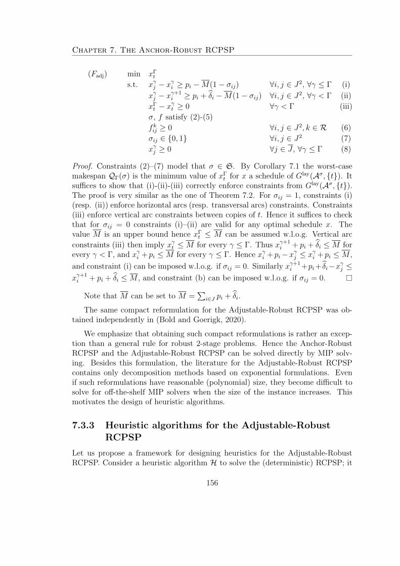
Chapter 7. The Anchor-Robust RCPSP
(Fadj) min xΓt
s.t. xγj − xγi ≥ pi −M(1− σij) ∀i, j ∈ J2, ∀γ ≤ Γ (i)
xγj − xγ+1i ≥ pi + δi −M(1− σij) ∀i, j ∈ J2, ∀γ < Γ (ii)
xΓt − x
γt ≥ 0 ∀γ < Γ (iii)
σ, f satisfy (2)-(5)
fkij ≥ 0 ∀i, j ∈ J2, k ∈ R (6)
σij ∈ {0, 1} ∀i, j ∈ J2 (7)
xγj ≥ 0 ∀j ∈ J , ∀γ ≤ Γ (8)
Proof. Constraints (2)–(7) model that σ ∈ S. By Corollary 7.1 the worst-casemakespan QΓ(σ) is the minimum value of xΓ
t for x a schedule of Glay(Aσ, {t}). Itsuffices to show that (i)-(ii)-(iii) correctly enforce constraints from Glay(Aσ, {t}).The proof is very similar as the one of Theorem 7.2. For σij = 1, constraints (i)(resp. (ii)) enforce horizontal arcs (resp. transversal arcs) constraints. Constraints(iii) enforce vertical arc constraints between copies of t. Hence it suffices to checkthat for σij = 0 constraints (i)–(ii) are valid for any optimal schedule x. Thevalue M is an upper bound hence xΓ
t ≤ M can be assumed w.l.o.g. Vertical arc
constraints (iii) then imply xγt ≤M for every γ ≤ Γ. Thus xγ+1i + pi + δi ≤M for
every γ < Γ, and xγi + pi ≤M for every γ ≤ Γ. Hence xγi + pi−xγj ≤ xγi + pi ≤M ,
and constraint (i) can be imposed w.l.o.g. if σij = 0. Similarly xγ+1i +pi+ δi−xγj ≤
xγ+1i + pi + δi ≤M , and constraint (b) can be imposed w.l.o.g. if σij = 0.
Note that M can be set to M =∑
i∈J pi + δi.
The same compact reformulation for the Adjustable-Robust RCPSP was ob-tained independently in (Bold and Goerigk, 2020).
We emphasize that obtaining such compact reformulations is rather an excep-tion than a general rule for robust 2-stage problems. Hence the Anchor-RobustRCPSP and the Adjustable-Robust RCPSP can be solved directly by MIP solv-ing. Besides this formulation, the literature for the Adjustable-Robust RCPSPcontains only decomposition methods based on exponential formulations. Evenif such reformulations have reasonable (polynomial) size, they become difficult tosolve for off-the-shelf MIP solvers when the size of the instance increases. Thismotivates the design of heuristic algorithms.
7.3.3 Heuristic algorithms for the Adjustable-RobustRCPSP
Let us propose a framework for designing heuristics for the Adjustable-RobustRCPSP. Consider a heuristic algorithm H to solve the (deterministic) RCPSP; it
156
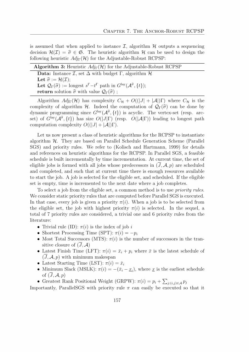
Chapter 7. The Anchor-Robust RCPSP
is assumed that when applied to instance I, algorithm H outputs a sequencingdecision H(I) = σ ∈ S. The heuristic algorithm H can be used to design thefollowing heuristic AdjΓ(H) for the Adjustable-Robust RCPSP:
Algorithm 3: Heuristic AdjΓ(H) for the Adjustable-Robust RCPSP
Data: Instance I, set ∆ with budget Γ, algorithm HLet σ := H(I);Let QΓ(σ) := longest sΓ−tΓ path in Glay(Aσ, {t});return solution σ with value QΓ(σ) ;
Algorithm AdjΓ(H) has complexity CH + O((|J | + |A|)Γ) where CH is thecomplexity of algorithm H. Indeed the computation of QΓ(σ) can be done bydynamic programming since Glay(Aσ, {t}) is acyclic. The vertex-set (resp. arc-set) of Glay(Aσ, {t}) has size O(|J |Γ) (resp. O(|A|Γ)) leading to longest pathcomputation complexity O((|J |+ |A|)Γ).
Let us now present a class of heuristic algorithms for the RCPSP to instantiatealgorithm H. They are based on Parallel Schedule Generation Scheme (ParallelSGS) and priority rules. We refer to (Kolisch and Hartmann, 1999) for detailsand references on heuristic algorithms for the RCPSP. In Parallel SGS, a feasibleschedule is built incrementally by time incrementation. At current time, the set ofeligible jobs is formed with all jobs whose predecessors in (J,A, p) are scheduledand completed, and such that at current time there is enough resources availableto start the job. A job is selected for the eligible set, and scheduled. If the eligibleset is empty, time is incremented to the next date where a job completes.
To select a job from the eligible set, a common method is to use priority rules.We consider static priority rules that are computed before Parallel SGS is executed.In that case, every job is given a priority π(i). When a job is to be selected fromthe eligible set, the job with highest priority π(i) is selected. In the sequel, atotal of 7 priority rules are considered, a trivial one and 6 priority rules from theliterature:
• Trivial rule (ID): π(i) is the index of job i• Shortest Processing Time (SPT): π(i) = −pi• Most Total Successors (MTS): π(i) is the number of successors in the tran-
sitive closure of (J,A)• Latest Finish Time (LFT): π(i) = xi + pi where x is the latest schedule of
(J,A, p) with minimum makespan• Latest Starting Time (LST): π(i) = xi• Minimum Slack (MSLK): π(i) = −(xi − xi), where x is the earliest schedule
of (J,A, p)• Greatest Rank Positional Weight (GRPW): π(i) = pi +
∑j:(i,j)∈A pj
Importantly, ParallelSGS with priority rule π can easily be executed so that it
157
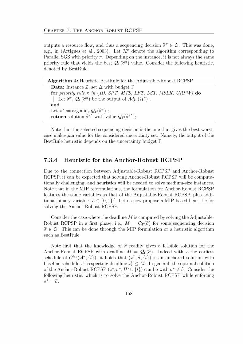
Chapter 7. The Anchor-Robust RCPSP
outputs a resource flow, and thus a sequencing decision σπ ∈ S. This was done,e.g., in (Artigues et al., 2003). Let Hπ denote the algorithm corresponding toParallel SGS with priority π. Depending on the instance, it is not always the samepriority rule that yields the best QΓ(σπ) value. Consider the following heuristic,denoted by BestRule:
Algorithm 4: Heuristic BestRule for the Adjustable-Robust RCPSP
Data: Instance I, set ∆ with budget Γfor priority rule π in {ID, SPT, MTS, LFT, LST, MSLK, GRPW} do
Let σπ, QΓ(σπ) be the output of AdjΓ(Hπ) ;endLet π∗ := arg minπQΓ(σπ) ;return solution σπ
∗with value QΓ(σπ
∗);
Note that the selected sequencing decision is the one that gives the best worst-case makespan value for the considered uncertainty set. Namely, the output of theBestRule heuristic depends on the uncertainty budget Γ.
7.3.4 Heuristic for the Anchor-Robust RCPSP
Due to the connection between Adjustable-Robust RCPSP and Anchor-RobustRCPSP, it can be expected that solving Anchor-Robust RCPSP will be computa-tionally challenging, and heuristics will be needed to solve medium-size instances.Note that in the MIP reformulations, the formulation for Anchor-Robust RCPSPfeatures the same variables as that of the Adjustable-Robust RCPSP, plus addi-tional binary variables h ∈ {0, 1}J . Let us now propose a MIP-based heuristic forsolving the Anchor-Robust RCPSP.
Consider the case where the deadline M is computed by solving the Adjustable-Robust RCPSP in a first phase, i.e., M = QΓ(σ) for some sequencing decisionσ ∈ S. This can be done through the MIP formulation or a heuristic algorithmsuch as BestRule.
Note first that the knowledge of σ readily gives a feasible solution for theAnchor-Robust RCPSP with deadline M = QΓ(σ). Indeed with x the earliestschedule of Glay(Aσ, {t}), it holds that (xΓ, σ, {t}) is an anchored solution withbaseline schedule xΓ respecting deadline xΓ
t ≤M . In general, the optimal solutionof the Anchor-Robust RCPSP (z∗, σ∗, H∗ ∪{t}) can be with σ∗ 6= σ. Consider thefollowing heuristic, which is to solve the Anchor-Robust RCPSP while enforcingσ∗ = σ:
158
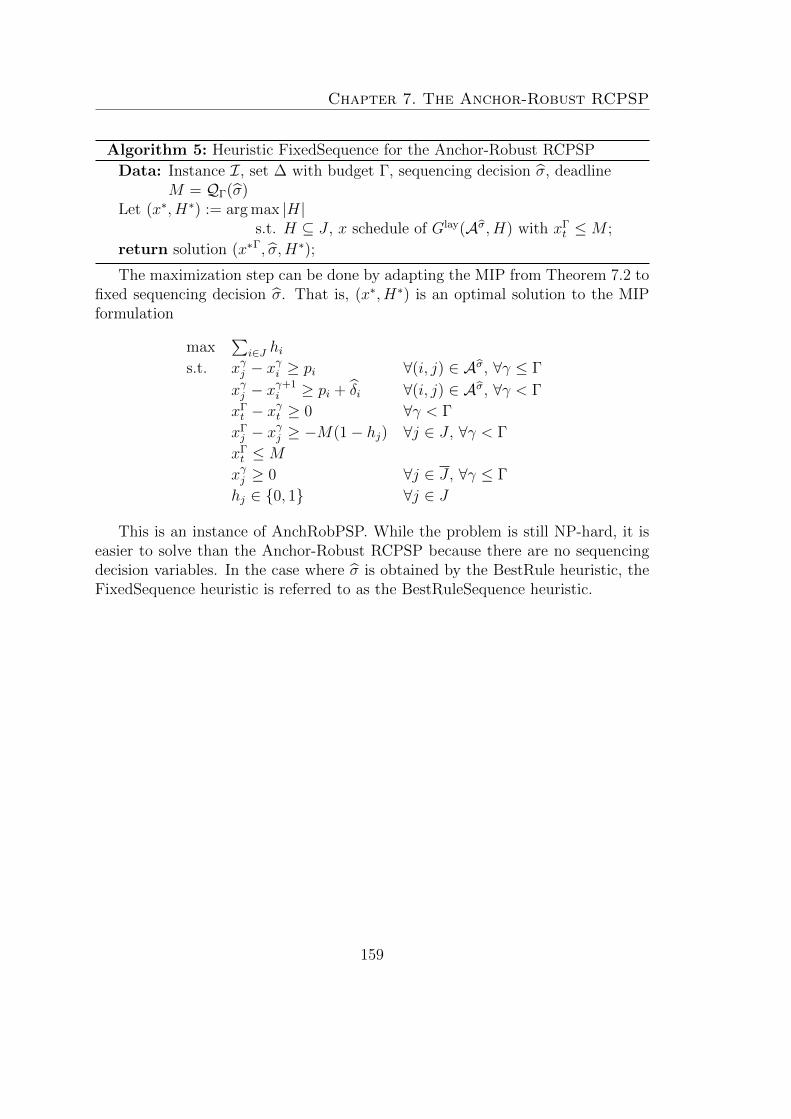
Chapter 7. The Anchor-Robust RCPSP
Algorithm 5: Heuristic FixedSequence for the Anchor-Robust RCPSP
Data: Instance I, set ∆ with budget Γ, sequencing decision σ, deadlineM = QΓ(σ)
Let (x∗, H∗) := arg max |H|s.t. H ⊆ J , x schedule of Glay(Aσ, H) with xΓ
t ≤M ;
return solution (x∗Γ, σ, H∗);
The maximization step can be done by adapting the MIP from Theorem 7.2 tofixed sequencing decision σ. That is, (x∗, H∗) is an optimal solution to the MIPformulation
max∑
i∈J his.t. xγj − x
γi ≥ pi ∀(i, j) ∈ Aσ, ∀γ ≤ Γ
xγj − xγ+1i ≥ pi + δi ∀(i, j) ∈ Aσ, ∀γ < Γ
xΓt − x
γt ≥ 0 ∀γ < Γ
xΓj − x
γj ≥ −M(1− hj) ∀j ∈ J , ∀γ < Γ
xΓt ≤M
xγj ≥ 0 ∀j ∈ J , ∀γ ≤ Γ
hj ∈ {0, 1} ∀j ∈ J
This is an instance of AnchRobPSP. While the problem is still NP-hard, it iseasier to solve than the Anchor-Robust RCPSP because there are no sequencingdecision variables. In the case where σ is obtained by the BestRule heuristic, theFixedSequence heuristic is referred to as the BestRuleSequence heuristic.
159
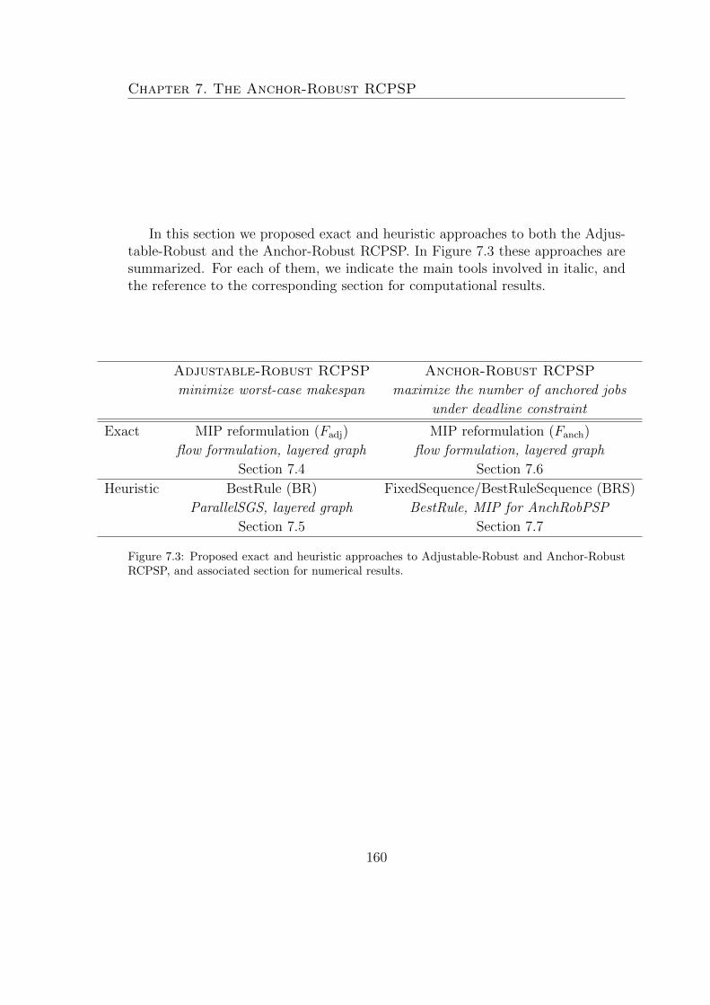
Chapter 7. The Anchor-Robust RCPSP
In this section we proposed exact and heuristic approaches to both the Adjus-table-Robust and the Anchor-Robust RCPSP. In Figure 7.3 these approaches aresummarized. For each of them, we indicate the main tools involved in italic, andthe reference to the corresponding section for computational results.
Adjustable-Robust RCPSP Anchor-Robust RCPSP
minimize worst-case makespan maximize the number of anchored jobs
under deadline constraint
Exact MIP reformulation (Fadj) MIP reformulation (Fanch)
flow formulation, layered graph flow formulation, layered graph
Section 7.4 Section 7.6
Heuristic BestRule (BR) FixedSequence/BestRuleSequence (BRS)
ParallelSGS, layered graph BestRule, MIP for AnchRobPSP
Section 7.5 Section 7.7
Figure 7.3: Proposed exact and heuristic approaches to Adjustable-Robust and Anchor-RobustRCPSP, and associated section for numerical results.
160
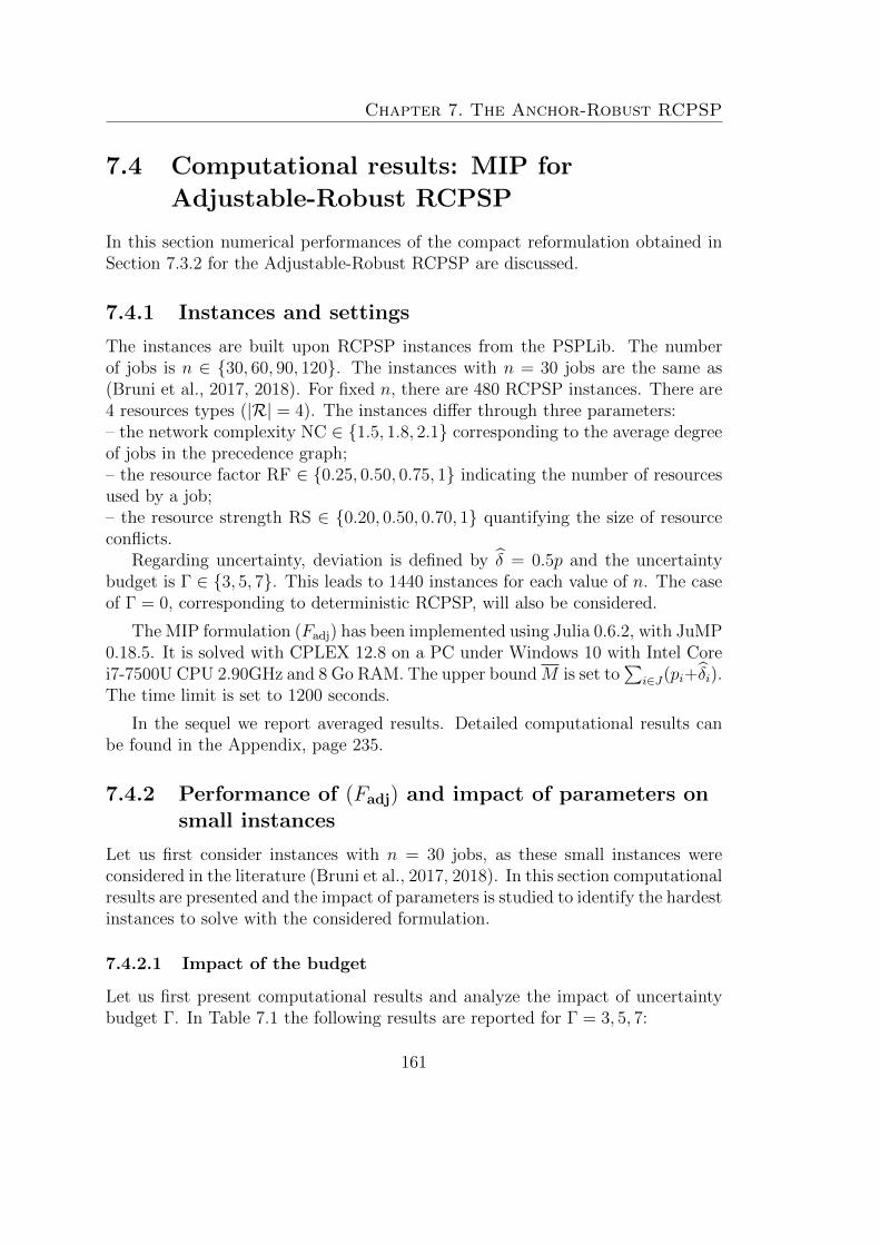
Chapter 7. The Anchor-Robust RCPSP
7.4 Computational results: MIP for
Adjustable-Robust RCPSP
In this section numerical performances of the compact reformulation obtained inSection 7.3.2 for the Adjustable-Robust RCPSP are discussed.
7.4.1 Instances and settings
The instances are built upon RCPSP instances from the PSPLib. The numberof jobs is n ∈ {30, 60, 90, 120}. The instances with n = 30 jobs are the same as(Bruni et al., 2017, 2018). For fixed n, there are 480 RCPSP instances. There are4 resources types (|R| = 4). The instances differ through three parameters:– the network complexity NC ∈ {1.5, 1.8, 2.1} corresponding to the average degreeof jobs in the precedence graph;– the resource factor RF ∈ {0.25, 0.50, 0.75, 1} indicating the number of resourcesused by a job;– the resource strength RS ∈ {0.20, 0.50, 0.70, 1} quantifying the size of resourceconflicts.
Regarding uncertainty, deviation is defined by δ = 0.5p and the uncertaintybudget is Γ ∈ {3, 5, 7}. This leads to 1440 instances for each value of n. The caseof Γ = 0, corresponding to deterministic RCPSP, will also be considered.
The MIP formulation (Fadj) has been implemented using Julia 0.6.2, with JuMP0.18.5. It is solved with CPLEX 12.8 on a PC under Windows 10 with Intel Corei7-7500U CPU 2.90GHz and 8 Go RAM. The upper boundM is set to
∑i∈J(pi+δi).
The time limit is set to 1200 seconds.
In the sequel we report averaged results. Detailed computational results canbe found in the Appendix, page 235.
7.4.2 Performance of (Fadj) and impact of parameters onsmall instances
Let us first consider instances with n = 30 jobs, as these small instances wereconsidered in the literature (Bruni et al., 2017, 2018). In this section computationalresults are presented and the impact of parameters is studied to identify the hardestinstances to solve with the considered formulation.
7.4.2.1 Impact of the budget
Let us first present computational results and analyze the impact of uncertaintybudget Γ. In Table 7.1 the following results are reported for Γ = 3, 5, 7:
161
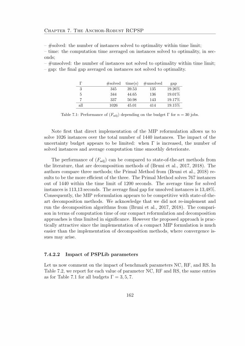
Chapter 7. The Anchor-Robust RCPSP
– #solved: the number of instances solved to optimality within time limit;– time: the computation time averaged on instances solved to optimality, in sec-onds;– #unsolved: the number of instances not solved to optimality within time limit;– gap: the final gap averaged on instances not solved to optimality.
Γ #solved time(s) #unsolved gap
3 345 39.53 135 19.26%
5 344 44.65 136 19.01%
7 337 50.98 143 19.17%
all 1026 45.01 414 19.15%
Table 7.1: Performance of (Fadj) depending on the budget Γ for n = 30 jobs.
Note first that direct implementation of the MIP reformulation allows us tosolve 1026 instances over the total number of 1440 instances. The impact of theuncertainty budget appears to be limited: when Γ is increased, the number ofsolved instances and average computation time smoothly deteriorate.
The performance of (Fadj) can be compared to state-of-the-art methods fromthe literature, that are decomposition methods of (Bruni et al., 2017, 2018). Theauthors compare three methods; the Primal Method from (Bruni et al., 2018) re-sults to be the more efficient of the three. The Primal Method solves 767 instancesout of 1440 within the time limit of 1200 seconds. The average time for solvedinstances is 113,13 seconds. The average final gap for unsolved instances is 13,48%.Consequently, the MIP reformulation appears to be competitive with state-of-the-art decomposition methods. We acknowledge that we did not re-implement andrun the decomposition algorithms from (Bruni et al., 2017, 2018). The compari-son in terms of computation time of our compact reformulation and decompositionapproaches is thus limited in significance. However the proposed approach is prac-tically attractive since the implementation of a compact MIP formulation is mucheasier than the implementation of decomposition methods, where convergence is-sues may arise.
7.4.2.2 Impact of PSPLib parameters
Let us now comment on the impact of benchmark parameters NC, RF, and RS. InTable 7.2, we report for each value of parameter NC, RF and RS, the same entriesas for Table 7.1 for all budgets Γ = 3, 5, 7.
162
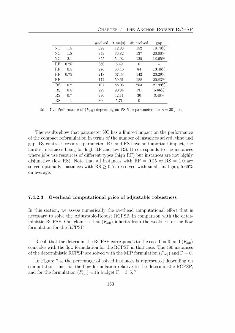
Chapter 7. The Anchor-Robust RCPSP
#solved time(s) #unsolved gap
NC 1.5 328 42.83 152 18.78%
NC 1.8 343 36.82 137 20.00%
NC 2.1 355 54.92 125 18.65%
RF 0.25 360 6.49 0 -
RF 0.5 276 68.46 84 13.46%
RF 0.75 218 67.38 142 20.29%
RF 1 172 59.61 188 20.83%
RS 0.2 107 88.05 253 27.99%
RS 0.5 229 90.84 131 5.66%
RS 0.7 330 42.11 30 3.48%
RS 1 360 5.71 0 -
Table 7.2: Performance of (Fadj) depending on PSPLib parameters for n = 30 jobs.
The results show that parameter NC has a limited impact on the performanceof the compact reformulation in terms of the number of instances solved, time andgap. By contrast, resource parameters RF and RS have an important impact, thehardest instances being for high RF and low RS. It corresponds to the instanceswhere jobs use resources of different types (high RF) but instances are not highlydisjunctive (low RS). Note that all instances with RF = 0.25 or RS = 1.0 aresolved optimally; instances with RS ≥ 0.5 are solved with small final gap, 5.66%on average.
7.4.2.3 Overhead computational price of adjustable robustness
In this section, we assess numerically the overhead computational effort that isnecessary to solve the Adjustable-Robust RCPSP, in comparison with the deter-ministic RCPSP. Our claim is that (Fadj) inherits from the weakness of the flowformulation for the RCPSP.
Recall that the deterministic RCPSP corresponds to the case Γ = 0, and (Fadj)coincides with the flow formulation for the RCPSP in that case. The 480 instancesof the deterministic RCPSP are solved with the MIP formulation (Fadj) and Γ = 0.
In Figure 7.4, the percentage of solved instances is represented depending oncomputation time, for the flow formulation relative to the deterministic RCPSP,and for the formulation (Fadj) with budget Γ = 3, 5, 7.
163
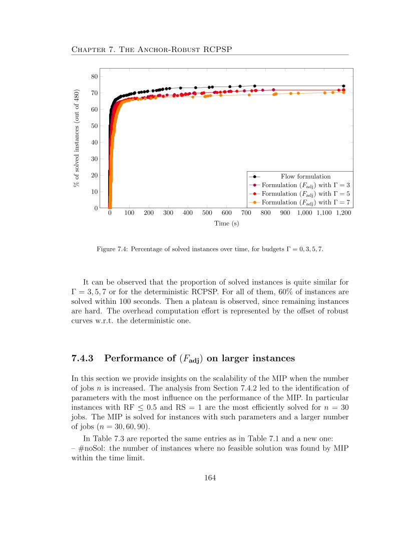
Chapter 7. The Anchor-Robust RCPSP
0 100 200 300 400 500 600 700 800 900 1,000 1,100 1,2000
10
20
30
40
50
60
70
80
Time (s)
%of
solv
edin
stan
ces
(ou
tof
480)
Flow formulation
Formulation (Fadj) with Γ = 3
Formulation (Fadj) with Γ = 5
Formulation (Fadj) with Γ = 7
Figure 7.4: Percentage of solved instances over time, for budgets Γ = 0, 3, 5, 7.
It can be observed that the proportion of solved instances is quite similar forΓ = 3, 5, 7 or for the deterministic RCPSP. For all of them, 60% of instances aresolved within 100 seconds. Then a plateau is observed, since remaining instancesare hard. The overhead computation effort is represented by the offset of robustcurves w.r.t. the deterministic one.
7.4.3 Performance of (Fadj) on larger instances
In this section we provide insights on the scalability of the MIP when the numberof jobs n is increased. The analysis from Section 7.4.2 led to the identification ofparameters with the most influence on the performance of the MIP. In particularinstances with RF ≤ 0.5 and RS = 1 are the most efficiently solved for n = 30jobs. The MIP is solved for instances with such parameters and a larger numberof jobs (n = 30, 60, 90).
In Table 7.3 are reported the same entries as in Table 7.1 and a new one:– #noSol: the number of instances where no feasible solution was found by MIPwithin the time limit.
164
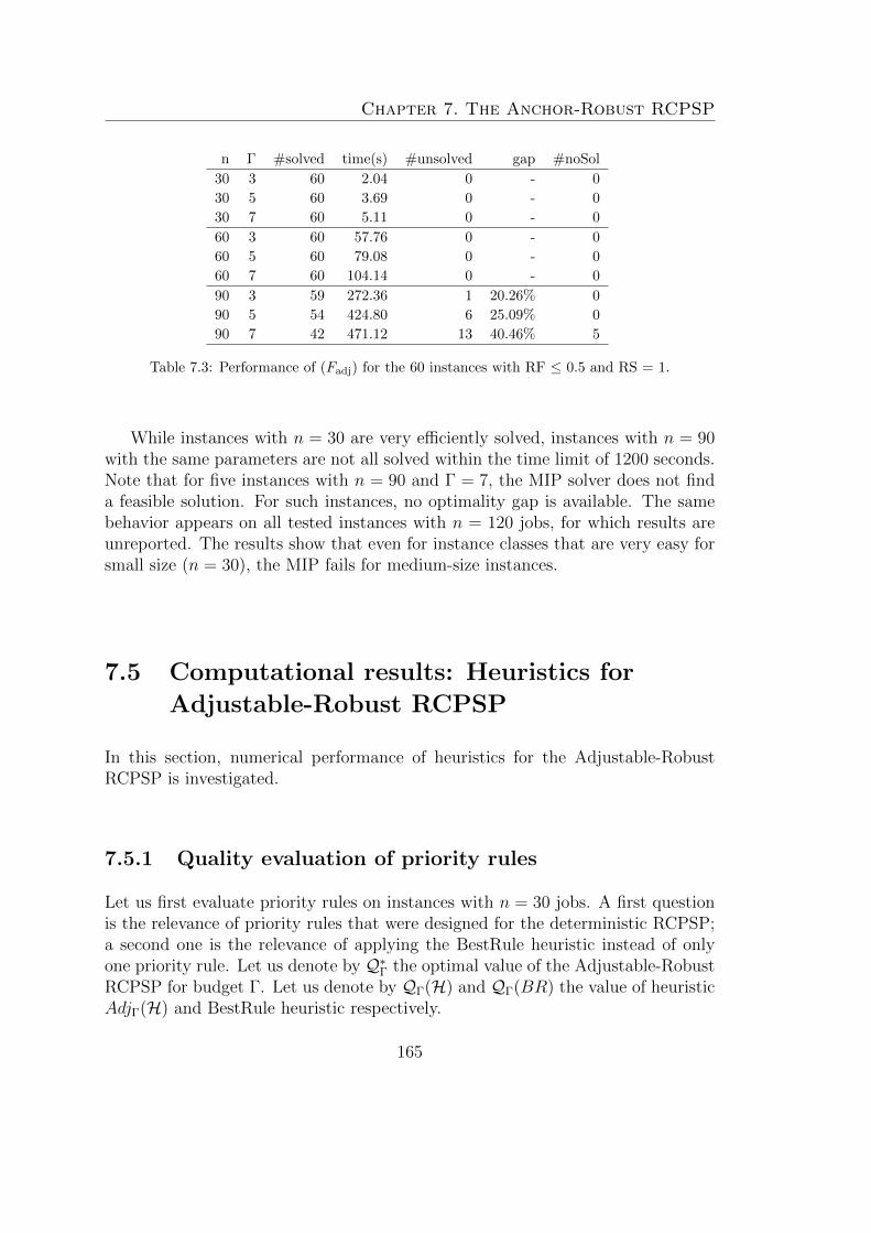
Chapter 7. The Anchor-Robust RCPSP
n Γ #solved time(s) #unsolved gap #noSol
30 3 60 2.04 0 - 0
30 5 60 3.69 0 - 0
30 7 60 5.11 0 - 0
60 3 60 57.76 0 - 0
60 5 60 79.08 0 - 0
60 7 60 104.14 0 - 0
90 3 59 272.36 1 20.26% 0
90 5 54 424.80 6 25.09% 0
90 7 42 471.12 13 40.46% 5
Table 7.3: Performance of (Fadj) for the 60 instances with RF ≤ 0.5 and RS = 1.
While instances with n = 30 are very efficiently solved, instances with n = 90with the same parameters are not all solved within the time limit of 1200 seconds.Note that for five instances with n = 90 and Γ = 7, the MIP solver does not finda feasible solution. For such instances, no optimality gap is available. The samebehavior appears on all tested instances with n = 120 jobs, for which results areunreported. The results show that even for instance classes that are very easy forsmall size (n = 30), the MIP fails for medium-size instances.
7.5 Computational results: Heuristics for
Adjustable-Robust RCPSP
In this section, numerical performance of heuristics for the Adjustable-RobustRCPSP is investigated.
7.5.1 Quality evaluation of priority rules
Let us first evaluate priority rules on instances with n = 30 jobs. A first questionis the relevance of priority rules that were designed for the deterministic RCPSP;a second one is the relevance of applying the BestRule heuristic instead of onlyone priority rule. Let us denote by Q∗Γ the optimal value of the Adjustable-RobustRCPSP for budget Γ. Let us denote by QΓ(H) and QΓ(BR) the value of heuristicAdjΓ(H) and BestRule heuristic respectively.
165
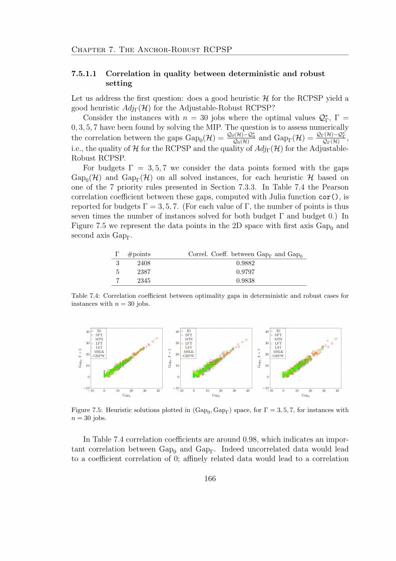
Chapter 7. The Anchor-Robust RCPSP
7.5.1.1 Correlation in quality between deterministic and robustsetting
Let us address the first question: does a good heuristic H for the RCPSP yield agood heuristic AdjΓ(H) for the Adjustable-Robust RCPSP?
Consider the instances with n = 30 jobs where the optimal values Q∗Γ, Γ =0, 3, 5, 7 have been found by solving the MIP. The question is to assess numerically
the correlation between the gaps Gap0(H) =Q0(H)−Q∗0Q0(H)
and GapΓ(H) =QΓ(H)−Q∗ΓQΓ(H)
,
i.e., the quality ofH for the RCPSP and the quality of AdjΓ(H) for the Adjustable-Robust RCPSP.
For budgets Γ = 3, 5, 7 we consider the data points formed with the gapsGap0(H) and GapΓ(H) on all solved instances, for each heuristic H based onone of the 7 priority rules presented in Section 7.3.3. In Table 7.4 the Pearsoncorrelation coefficient between these gaps, computed with Julia function cor(), isreported for budgets Γ = 3, 5, 7. (For each value of Γ, the number of points is thusseven times the number of instances solved for both budget Γ and budget 0.) InFigure 7.5 we represent the data points in the 2D space with first axis Gap0 andsecond axis GapΓ.
Γ #points Correl. Coeff. between GapΓ and Gap0
3 2408 0.9882
5 2387 0.9797
7 2345 0.9838
Table 7.4: Correlation coefficient between optimality gaps in deterministic and robust cases forinstances with n = 30 jobs.
−10 0 10 20 30 40−10
0
10
20
30
40
Gap0
Gap
Γ,
Γ=
3
IDSPTMTSLFTLST
MSLKGRPW
−10 0 10 20 30 40−10
0
10
20
30
40
Gap0
Gap
Γ,
Γ=
5
IDSPTMTSLFTLST
MSLKGRPW
−10 0 10 20 30 40−10
0
10
20
30
40
Gap0
Gap
Γ,
Γ=
7
IDSPTMTSLFTLST
MSLKGRPW
Figure 7.5: Heuristic solutions plotted in (Gap0,GapΓ) space, for Γ = 3, 5, 7, for instances withn = 30 jobs.
In Table 7.4 correlation coefficients are around 0.98, which indicates an impor-tant correlation between Gap0 and GapΓ. Indeed uncorrelated data would leadto a coefficient correlation of 0; affinely related data would lead to a correlation
166
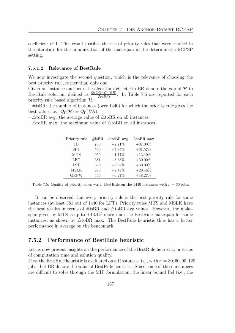
Chapter 7. The Anchor-Robust RCPSP
coefficient of 1. This result justifies the use of priority rules that were studied inthe literature for the minimization of the makespan in the deterministic RCPSPsetting.
7.5.1.2 Relevance of BestRule
We now investigate the second question, which is the relevance of choosing thebest priority rule, rather than only one.Given an instance and heuristic algorithm H, let 4toBR denote the gap of H toBestRule solution, defined as QΓ(H)−QΓ(BR)
QΓ(BR). In Table 7.5 are reported for each
priority rule based algorithm H:– #isBR: the number of instances (over 1440) for which the priority rule gives thebest value, i.e., QΓ(H) = QΓ(BR);– 4toBR avg: the average value of 4toBR on all instances;– 4toBR max: the maximum value of 4toBR on all instances.
Priority rule #isBR 4toBR avg 4toBR max
ID 703 +2.71% +37.00%
SPT 540 +4.85% +31.57%
MTS 959 +1.17% +13.40%
LFT 381 +8.38% +50.00%
LST 398 +8.32% +50.00%
MSLK 866 +2.48% +29.46%
GRPW 446 +6.27% +48.27%
Table 7.5: Quality of priority rules w.r.t. BestRule on the 1440 instances with n = 30 jobs.
It can be observed that every priority rule is the best priority rule for someinstances (at least 381 out of 1440 for LFT). Priority rules MTS and MSLK havethe best results in terms of #isBR and 4toBR avg values. However, the make-span given by MTS is up to +13.4% more than the BestRule makespan for someinstances, as shown by 4toBR max. The BestRule heuristic thus has a betterperformance in average on the benchmark.
7.5.2 Performance of BestRule heuristic
Let us now present insights on the performance of the BestRule heuristic, in termsof computation time and solution quality.First the BestRule heuristic is evaluated on all instances, i.e., with n = 30, 60, 90, 120jobs. Let BR denote the value of BestRule heuristic. Since some of these instancesare difficult to solve through the MIP formulation, the linear bound Rel (i.e., the
167
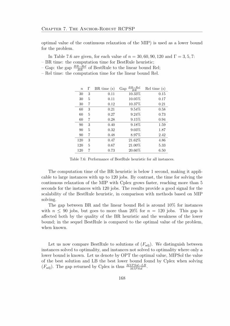
Chapter 7. The Anchor-Robust RCPSP
optimal value of the continuous relaxation of the MIP) is used as a lower boundfor the problem.
In Table 7.6 are given, for each value of n = 30, 60, 90, 120 and Γ = 3, 5, 7:– BR time: the computation time for BestRule heuristic;– Gap: the gap BR−Rel
BRof BestRule to the linear bound Rel;
– Rel time: the computation time for the linear bound Rel.
n Γ BR time (s) Gap BR−RelBR Rel time (s)
30 3 0.11 10.33% 0.15
30 5 0.11 10.05% 0.17
30 7 0.12 10.37% 0.21
60 3 0.21 9.54% 0.58
60 5 0.27 9.24% 0.73
60 7 0.28 9.15% 0.94
90 3 0.40 9.18% 1.59
90 5 0.32 9.03% 1.87
90 7 0.48 8.97% 2.42
120 3 0.47 21.62% 4.86
120 5 0.67 21.00% 5.33
120 7 0.73 20.66% 6.50
Table 7.6: Performance of BestRule heuristic for all instances.
The computation time of the BR heuristic is below 1 second, making it appli-cable to large instances with up to 120 jobs. By contrast, the time for solving thecontinuous relaxation of the MIP with Cplex grows faster, reaching more than 5seconds for the instances with 120 jobs. The results provide a good signal for thescalability of the BestRule heuristic, in comparison with methods based on MIPsolving.
The gap between BR and the linear bound Rel is around 10% for instanceswith n ≤ 90 jobs, but goes to more than 20% for n = 120 jobs. This gap isaffected both by the quality of the BR heuristic and the weakness of the lowerbound; in the sequel BestRule is compared to the optimal value of the problem,when known.
Let us now compare BestRule to solutions of (Fadj). We distinguish betweeninstances solved to optimality, and instances not solved to optimality where only alower bound is known. Let us denote by OPT the optimal value, MIPSol the valueof the best solution and LB the best lower bound found by Cplex when solving(Fadj). The gap returned by Cplex is thus MIPSol−LB
MIPSol.
168
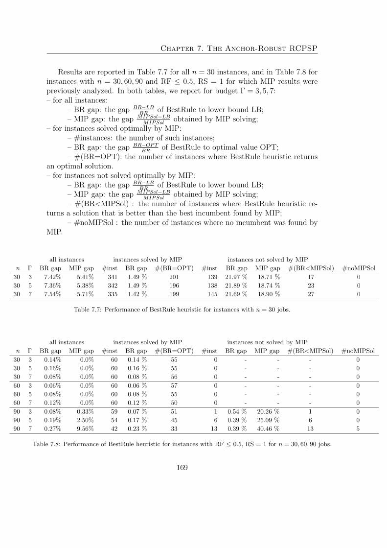
Chapter 7. The Anchor-Robust RCPSP
Results are reported in Table 7.7 for all n = 30 instances, and in Table 7.8 forinstances with n = 30, 60, 90 and RF ≤ 0.5, RS = 1 for which MIP results werepreviously analyzed. In both tables, we report for budget Γ = 3, 5, 7:– for all instances:
– BR gap: the gap BR−LBBR
of BestRule to lower bound LB;– MIP gap: the gap MIPSol−LB
MIPSolobtained by MIP solving;
– for instances solved optimally by MIP:– #instances: the number of such instances;– BR gap: the gap BR−OPT
BRof BestRule to optimal value OPT;
– #(BR=OPT): the number of instances where BestRule heuristic returnsan optimal solution.– for instances not solved optimally by MIP:
– BR gap: the gap BR−LBBR
of BestRule to lower bound LB;– MIP gap: the gap MIPSol−LB
MIPSolobtained by MIP solving;
– #(BR<MIPSol) : the number of instances where BestRule heuristic re-turns a solution that is better than the best incumbent found by MIP;
– #noMIPSol : the number of instances where no incumbent was found byMIP.
all instances instances solved by MIP instances not solved by MIP
n Γ BR gap MIP gap #inst BR gap #(BR=OPT) #inst BR gap MIP gap #(BR<MIPSol) #noMIPSol
30 3 7.42% 5.41% 341 1.49 % 201 139 21.97 % 18.71 % 17 0
30 5 7.36% 5.38% 342 1.49 % 196 138 21.89 % 18.74 % 23 0
30 7 7.54% 5.71% 335 1.42 % 199 145 21.69 % 18.90 % 27 0
Table 7.7: Performance of BestRule heuristic for instances with n = 30 jobs.
all instances instances solved by MIP instances not solved by MIP
n Γ BR gap MIP gap #inst BR gap #(BR=OPT) #inst BR gap MIP gap #(BR<MIPSol) #noMIPSol
30 3 0.14% 0.0% 60 0.14 % 55 0 - - - 0
30 5 0.16% 0.0% 60 0.16 % 55 0 - - - 0
30 7 0.08% 0.0% 60 0.08 % 56 0 - - - 0
60 3 0.06% 0.0% 60 0.06 % 57 0 - - - 0
60 5 0.08% 0.0% 60 0.08 % 55 0 - - - 0
60 7 0.12% 0.0% 60 0.12 % 50 0 - - - 0
90 3 0.08% 0.33% 59 0.07 % 51 1 0.54 % 20.26 % 1 0
90 5 0.19% 2.50% 54 0.17 % 45 6 0.39 % 25.09 % 6 0
90 7 0.27% 9.56% 42 0.23 % 33 13 0.39 % 40.46 % 13 5
Table 7.8: Performance of BestRule heuristic for instances with RF ≤ 0.5, RS = 1 for n = 30, 60, 90 jobs.
169
Chapter 7. The Anchor-Robust RCPSP
In Table 7.7 it can be observed that the BR gap is at most 7.54% on average;BR gap is around 2% larger than the MIP gap. For instances where OPT is known,BR gap is even smaller (at most 1.49%). Notably, BestRule outputs an optimalsolution on a large subset of instances: 596 out of 1440. For instances where OPTis not known, the BR gap is also close to MIP gap. On 67 instances, BestRuleoutputs a solution which is better than the best incumbent found by MIP solvingafter 1200 seconds computation.
In Table 7.8, similar results are obtained for instances with n = 30, 60 jobs,where OPT is known for all instances. The BR gap is very small (at most 0.14%on average), and BestRule gives an optimal solution for 328 instances out of 360.For n = 90 jobs, not all instances are solved by MIP. The BR gap is still very smallfor instances solved (at most 0.23% on average), and BestRule gives an optimalsolution for 130 instances out of 180. For instances where OPT is not known,the BestRule heuristic is very efficient (BR gap ≤ 1%), while MIP gap is large(more than 20%). The BestRule is better than the best MIP solution on all theseinstances. Note also that for Γ = 7, there are 5 instances where no MIP solutionwas known, while BestRule does provide a solution. The good performance ofBestRule on unsolved instances results into a very good performance on averageon all instances: e.g., for Γ = 7, BR gap is only 0.27% versus a MIP gap of 9.56%.
170
Chapter 7. The Anchor-Robust RCPSP
7.6 Computational results: MIP for
Anchor-Robust RCPSP
In this section, the compact MIP reformulation (Fanch) for Anchor-Robust RCPSPis evaluated. The impact of deadline M on the number of anchored jobs is alsodiscussed.
7.6.1 Instances and settings
Let us describe the settings of numerical experiments.The Anchor-Robust RCPSP instances are defined as follows. The instances of theRCPSP and uncertainty sets are the same as in Section 7.4. The only additionalinput of the Anchor-Robust RCPSP is the deadline M . As proposed in Section 7.2,the deadline M can be found by solving the Adjustable-Robust RCPSP. Since theAdjustable-Robust RCPSP is difficult to solve even for some instances with n = 30jobs, we consider in the sequel that deadline M is set to the value M = QΓ(BR)of BestRule heuristic. The BestRule heuristic is thus applied on each instance todetermine M . The solution found by BestRule heuristic is a sequencing decisionσ with worst-case makespan QΓ(σ) = M . The sequencing decision σ ∈ S is fed to(Fanch) as a warm-start. Note that this gives a feasible solution to the MIP solver,with hi = 0 for every i ∈ J .
Computational settings are the same as in Section 7.4. The time limit for MIPsolving is set to 1200 seconds. The computation times reported in this section donot include the computation time of BestRule heuristic, which is negligible w.r.t.MIP solving.
7.6.2 Performance of (Fanch) on small instances
Let us first assess the performance of the compact reformulation (Fanch) for in-stances with n = 30 jobs, and analyze the influence of parameters.
In Table 7.9 and Table 7.10 are reported, for each value of Γ = 3, 5, 7 and foreach value of parameter NC, RF and RS respectively:– Anch: the average number of anchored jobs in the best solution found by (Fanch);– #solved: the number of instances solved to optimality within time limit;– time: the computation time averaged on instances solved to optimality, in sec-onds;– #unsolved: the number of instances not solved to optimality within time limit;– gap: the final gap averaged on instances not solved to optimality. It equalsUB−AnchAnch
where UB is the best upper bound found by MIP;
171
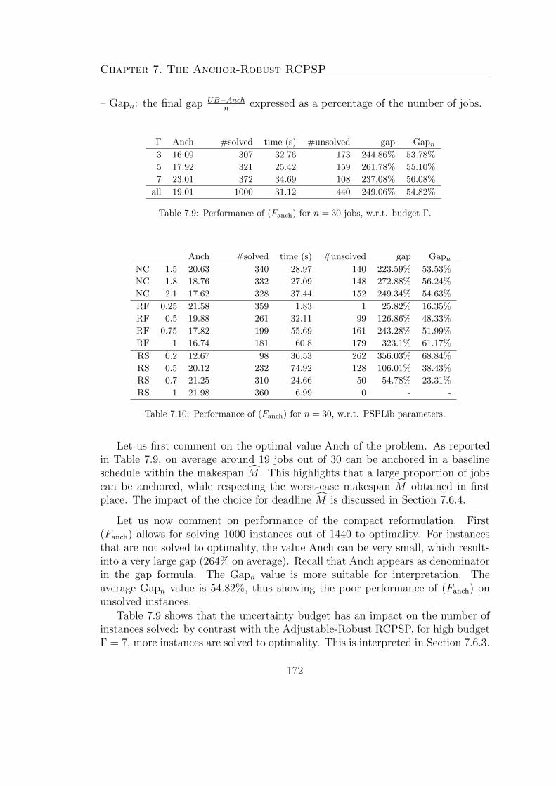
Chapter 7. The Anchor-Robust RCPSP
– Gapn: the final gap UB−Anchn
expressed as a percentage of the number of jobs.
Γ Anch #solved time (s) #unsolved gap Gapn3 16.09 307 32.76 173 244.86% 53.78%
5 17.92 321 25.42 159 261.78% 55.10%
7 23.01 372 34.69 108 237.08% 56.08%
all 19.01 1000 31.12 440 249.06% 54.82%
Table 7.9: Performance of (Fanch) for n = 30 jobs, w.r.t. budget Γ.
Anch #solved time (s) #unsolved gap GapnNC 1.5 20.63 340 28.97 140 223.59% 53.53%
NC 1.8 18.76 332 27.09 148 272.88% 56.24%
NC 2.1 17.62 328 37.44 152 249.34% 54.63%
RF 0.25 21.58 359 1.83 1 25.82% 16.35%
RF 0.5 19.88 261 32.11 99 126.86% 48.33%
RF 0.75 17.82 199 55.69 161 243.28% 51.99%
RF 1 16.74 181 60.8 179 323.1% 61.17%
RS 0.2 12.67 98 36.53 262 356.03% 68.84%
RS 0.5 20.12 232 74.92 128 106.01% 38.43%
RS 0.7 21.25 310 24.66 50 54.78% 23.31%
RS 1 21.98 360 6.99 0 - -
Table 7.10: Performance of (Fanch) for n = 30, w.r.t. PSPLib parameters.
Let us first comment on the optimal value Anch of the problem. As reportedin Table 7.9, on average around 19 jobs out of 30 can be anchored in a baselineschedule within the makespan M . This highlights that a large proportion of jobscan be anchored, while respecting the worst-case makespan M obtained in firstplace. The impact of the choice for deadline M is discussed in Section 7.6.4.
Let us now comment on performance of the compact reformulation. First(Fanch) allows for solving 1000 instances out of 1440 to optimality. For instancesthat are not solved to optimality, the value Anch can be very small, which resultsinto a very large gap (264% on average). Recall that Anch appears as denominatorin the gap formula. The Gapn value is more suitable for interpretation. Theaverage Gapn value is 54.82%, thus showing the poor performance of (Fanch) onunsolved instances.
Table 7.9 shows that the uncertainty budget has an impact on the number ofinstances solved: by contrast with the Adjustable-Robust RCPSP, for high budgetΓ = 7, more instances are solved to optimality. This is interpreted in Section 7.6.3.
172
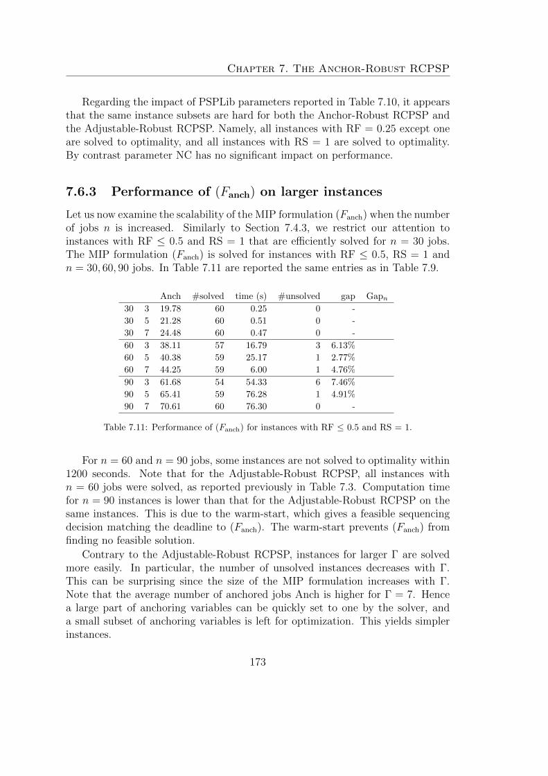
Chapter 7. The Anchor-Robust RCPSP
Regarding the impact of PSPLib parameters reported in Table 7.10, it appearsthat the same instance subsets are hard for both the Anchor-Robust RCPSP andthe Adjustable-Robust RCPSP. Namely, all instances with RF = 0.25 except oneare solved to optimality, and all instances with RS = 1 are solved to optimality.By contrast parameter NC has no significant impact on performance.
7.6.3 Performance of (Fanch) on larger instances
Let us now examine the scalability of the MIP formulation (Fanch) when the numberof jobs n is increased. Similarly to Section 7.4.3, we restrict our attention toinstances with RF ≤ 0.5 and RS = 1 that are efficiently solved for n = 30 jobs.The MIP formulation (Fanch) is solved for instances with RF ≤ 0.5, RS = 1 andn = 30, 60, 90 jobs. In Table 7.11 are reported the same entries as in Table 7.9.
Anch #solved time (s) #unsolved gap Gapn30 3 19.78 60 0.25 0 -
30 5 21.28 60 0.51 0 -
30 7 24.48 60 0.47 0 -
60 3 38.11 57 16.79 3 6.13%
60 5 40.38 59 25.17 1 2.77%
60 7 44.25 59 6.00 1 4.76%
90 3 61.68 54 54.33 6 7.46%
90 5 65.41 59 76.28 1 4.91%
90 7 70.61 60 76.30 0 -
Table 7.11: Performance of (Fanch) for instances with RF ≤ 0.5 and RS = 1.
For n = 60 and n = 90 jobs, some instances are not solved to optimality within1200 seconds. Note that for the Adjustable-Robust RCPSP, all instances withn = 60 jobs were solved, as reported previously in Table 7.3. Computation timefor n = 90 instances is lower than that for the Adjustable-Robust RCPSP on thesame instances. This is due to the warm-start, which gives a feasible sequencingdecision matching the deadline to (Fanch). The warm-start prevents (Fanch) fromfinding no feasible solution.
Contrary to the Adjustable-Robust RCPSP, instances for larger Γ are solvedmore easily. In particular, the number of unsolved instances decreases with Γ.This can be surprising since the size of the MIP formulation increases with Γ.Note that the average number of anchored jobs Anch is higher for Γ = 7. Hencea large part of anchoring variables can be quickly set to one by the solver, anda small subset of anchoring variables is left for optimization. This yields simplerinstances.
173
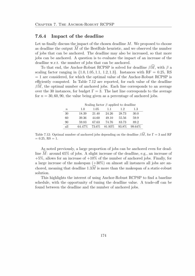
Chapter 7. The Anchor-Robust RCPSP
7.6.4 Impact of the deadline
Let us finally discuss the impact of the chosen deadline M . We proposed to chooseas deadline the output M of the BestRule heuristic, and we observed the numberof jobs that can be anchored. The deadline may also be increased, so that morejobs can be anchored. A question is to evaluate the impact of an increase of thedeadline w.r.t. the number of jobs that can be anchored.
To that end, the Anchor-Robust RCPSP is solved for deadline βM , with β ascaling factor ranging in {1.0, 1.05, 1.1, 1.2, 1.3}. Instances with RF = 0.25, RS= 1 are considered, for which the optimal value of the Anchor-Robust RCPSP isefficiently computed. In Table 7.12 are reported, for each value of the deadlineβM , the optimal number of anchored jobs. Each line corresponds to an averageover the 30 instances, for budget Γ = 3. The last line corresponds to the averagefor n = 30, 60, 90, the value being given as a percentage of anchored jobs.
Scaling factor β applied to deadline
n 1.0 1.05 1.1 1.2 1.3
30 18.39 21.40 24.26 28.73 30.0
60 39.36 44.60 49.10 55.56 59.9
90 59.83 67.63 74.76 83.73 89.2
all 64.47% 73.6% 81.93% 93.8% 99.64%
Table 7.12: Optimal number of anchored jobs depending on the deadline βM , for Γ = 3 and RF= 0.25, RS = 1.
As noted previously, a large proportion of jobs can be anchored even for dead-line M : around 65% of jobs. A slight increase of the deadline, e.g., an increase of+5%, allows for an increase of +10% of the number of anchored jobs. Finally, fora large increase of the makespan (+30%) on almost all instances all jobs are an-
chored, meaning that deadline 1.3M is more than the makespan of a static-robustsolution.
This highlights the interest of using Anchor-Robust RCPSP to find a baselineschedule, with the opportunity of tuning the deadline value. A trade-off can befound between the deadline and the number of anchored jobs.
174
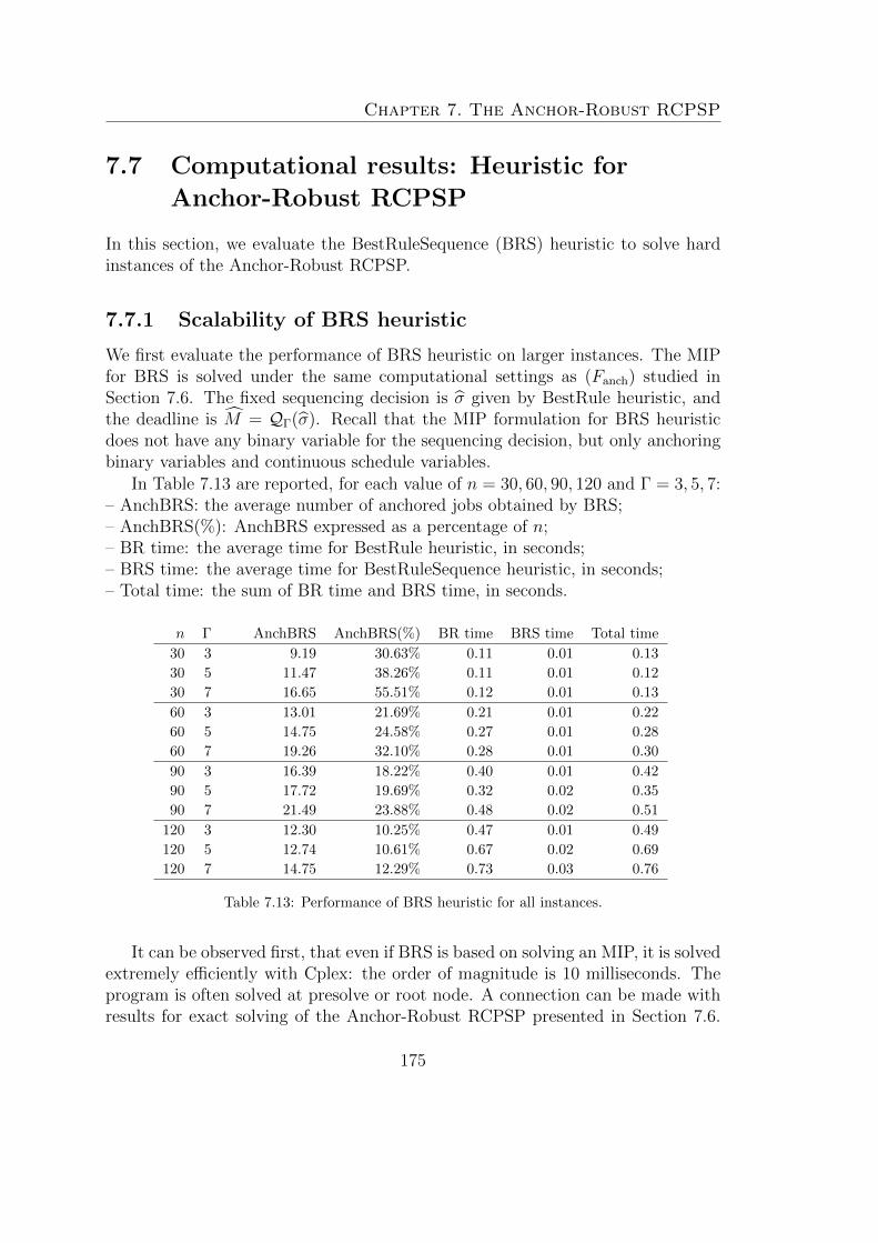
Chapter 7. The Anchor-Robust RCPSP
7.7 Computational results: Heuristic for
Anchor-Robust RCPSP
In this section, we evaluate the BestRuleSequence (BRS) heuristic to solve hardinstances of the Anchor-Robust RCPSP.
7.7.1 Scalability of BRS heuristic
We first evaluate the performance of BRS heuristic on larger instances. The MIPfor BRS is solved under the same computational settings as (Fanch) studied inSection 7.6. The fixed sequencing decision is σ given by BestRule heuristic, andthe deadline is M = QΓ(σ). Recall that the MIP formulation for BRS heuristicdoes not have any binary variable for the sequencing decision, but only anchoringbinary variables and continuous schedule variables.
In Table 7.13 are reported, for each value of n = 30, 60, 90, 120 and Γ = 3, 5, 7:– AnchBRS: the average number of anchored jobs obtained by BRS;– AnchBRS(%): AnchBRS expressed as a percentage of n;– BR time: the average time for BestRule heuristic, in seconds;– BRS time: the average time for BestRuleSequence heuristic, in seconds;– Total time: the sum of BR time and BRS time, in seconds.
n Γ AnchBRS AnchBRS(%) BR time BRS time Total time
30 3 9.19 30.63% 0.11 0.01 0.13
30 5 11.47 38.26% 0.11 0.01 0.12
30 7 16.65 55.51% 0.12 0.01 0.13
60 3 13.01 21.69% 0.21 0.01 0.22
60 5 14.75 24.58% 0.27 0.01 0.28
60 7 19.26 32.10% 0.28 0.01 0.30
90 3 16.39 18.22% 0.40 0.01 0.42
90 5 17.72 19.69% 0.32 0.02 0.35
90 7 21.49 23.88% 0.48 0.02 0.51
120 3 12.30 10.25% 0.47 0.01 0.49
120 5 12.74 10.61% 0.67 0.02 0.69
120 7 14.75 12.29% 0.73 0.03 0.76
Table 7.13: Performance of BRS heuristic for all instances.
It can be observed first, that even if BRS is based on solving an MIP, it is solvedextremely efficiently with Cplex: the order of magnitude is 10 milliseconds. Theprogram is often solved at presolve or root node. A connection can be made withresults for exact solving of the Anchor-Robust RCPSP presented in Section 7.6.
175
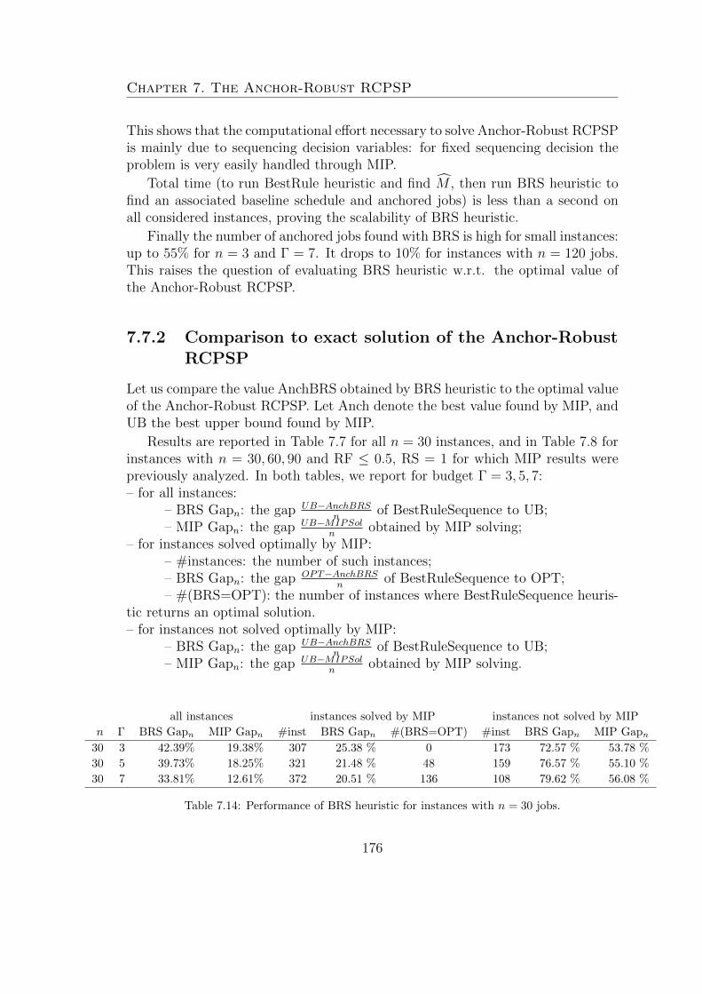
Chapter 7. The Anchor-Robust RCPSP
This shows that the computational effort necessary to solve Anchor-Robust RCPSPis mainly due to sequencing decision variables: for fixed sequencing decision theproblem is very easily handled through MIP.
Total time (to run BestRule heuristic and find M , then run BRS heuristic tofind an associated baseline schedule and anchored jobs) is less than a second onall considered instances, proving the scalability of BRS heuristic.
Finally the number of anchored jobs found with BRS is high for small instances:up to 55% for n = 3 and Γ = 7. It drops to 10% for instances with n = 120 jobs.This raises the question of evaluating BRS heuristic w.r.t. the optimal value ofthe Anchor-Robust RCPSP.
7.7.2 Comparison to exact solution of the Anchor-RobustRCPSP
Let us compare the value AnchBRS obtained by BRS heuristic to the optimal valueof the Anchor-Robust RCPSP. Let Anch denote the best value found by MIP, andUB the best upper bound found by MIP.
Results are reported in Table 7.7 for all n = 30 instances, and in Table 7.8 forinstances with n = 30, 60, 90 and RF ≤ 0.5, RS = 1 for which MIP results werepreviously analyzed. In both tables, we report for budget Γ = 3, 5, 7:– for all instances:
– BRS Gapn: the gap UB−AnchBRSn
of BestRuleSequence to UB;– MIP Gapn: the gap UB−MIPSol
nobtained by MIP solving;
– for instances solved optimally by MIP:– #instances: the number of such instances;– BRS Gapn: the gap OPT−AnchBRS
nof BestRuleSequence to OPT;
– #(BRS=OPT): the number of instances where BestRuleSequence heuris-tic returns an optimal solution.– for instances not solved optimally by MIP:
– BRS Gapn: the gap UB−AnchBRSn
of BestRuleSequence to UB;– MIP Gapn: the gap UB−MIPSol
nobtained by MIP solving.
all instances instances solved by MIP instances not solved by MIP
n Γ BRS Gapn MIP Gapn #inst BRS Gapn #(BRS=OPT) #inst BRS Gapn MIP Gapn30 3 42.39% 19.38% 307 25.38 % 0 173 72.57 % 53.78 %
30 5 39.73% 18.25% 321 21.48 % 48 159 76.57 % 55.10 %
30 7 33.81% 12.61% 372 20.51 % 136 108 79.62 % 56.08 %
Table 7.14: Performance of BRS heuristic for instances with n = 30 jobs.
176
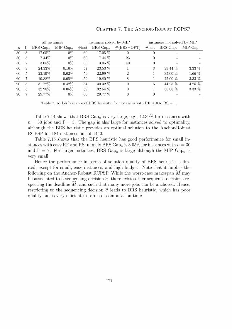
Chapter 7. The Anchor-Robust RCPSP
all instances instances solved by MIP instances not solved by MIP
n Γ BRS Gapn MIP Gapn #inst BRS Gapn #(BRS=OPT) #inst BRS Gapn MIP Gapn30 3 17.05% 0% 60 17.05 % 0 0 - -
30 5 7.44% 0% 60 7.44 % 23 0 - -
30 7 3.05% 0% 60 3.05 % 40 0 - -
60 3 24.33% 0.16% 57 23.53 % 1 3 39.44 % 3.33 %
60 5 23.19% 0.02% 59 22.99 % 2 1 35.00 % 1.66 %
60 7 19.88% 0.05% 59 19.80 % 8 1 25.00 % 3.33 %
90 3 31.72% 0.42% 54 30.32 % 0 6 44.25 % 4.25 %
90 5 32.98% 0.05% 59 32.54 % 0 1 58.88 % 3.33 %
90 7 29.77% 0% 60 29.77 % 0 0 - -
Table 7.15: Performance of BRS heuristic for instances with RF ≤ 0.5, RS = 1.
Table 7.14 shows that BRS Gapn is very large, e.g., 42.39% for instances withn = 30 jobs and Γ = 3. The gap is also large for instances solved to optimality,although the BRS heuristic provides an optimal solution to the Anchor-RobustRCPSP for 184 instances out of 1440.
Table 7.15 shows that the BRS heuristic has good performance for small in-stances with easy RF and RS: namely BRS Gapn is 3.05% for instances with n = 30and Γ = 7. For larger instances, BRS Gapn is large although the MIP Gapn isvery small.
Hence the performance in terms of solution quality of BRS heuristic is lim-ited, except for small, easy instances, and high budget. Note that it implies thefollowing on the Anchor-Robust RCPSP. While the worst-case makespan M maybe associated to a sequencing decision σ, there exists other sequence decisions re-specting the deadline M , and such that many more jobs can be anchored. Hence,restricting to the sequencing decision σ leads to BRS heuristic, which has poorquality but is very efficient in terms of computation time.
177
Chapter 7. The Anchor-Robust RCPSP
Conclusion
In the present work, the concept of anchor-robustness was applied to the RCPSP.The definition of anchored solutions generalizes the definition of solutions of theadjustable-robust approach. It offers a guarantee of starting times, in addition toa guarantee of the worst-case makespan, against realizations of processing times inthe uncertainty set. Anchor-robustness bridges the gap between static robustnessand adjustable robustness from the literature.
We extended a graph model designed for PERT scheduling and obtained resultsfor the Anchor-Robust RCPSP and the Adjustable-Robust RCPSP, leading toboth exact and heuristic approaches. Regarding exact solution approaches, weobtained compact MIP formulations for both problems. For heuristics, we showedhow to benefit from efficient heuristics for the RCPSP to design efficient heuristicsfor Anchor-Robust and Adjustable-Robust RCPSP. Altogether this is a completetoolbox for solving the Anchor-Robust and the Adjustable-Robust RCPSP.
A numerical evaluation of the proposed tools was performed. The compact re-formulation for the Adjustable-Robust RCPSP is competitive with decompositionalgorithms from the literature. We studied the scalability of MIPs, and identifiedhard instances. It turns out that these are the same as for the RCPSP, where opti-mizing the resource sequencing decision is computationally challenging. To addresssuch hard instances, the proposed heuristics are very efficient. The Anchor-RobustRCPSP can also be efficiently solved. In particular, the combination of BestRuleand BestRuleSequence heuristics provides both a robust makespan and baselineschedule with anchored jobs.
An important perspective is to improve MIP formulations. As illustrated innumerical experiments, the computational difficulty mainly arises from the binaryvariables for the sequencing decision. A question is to improve the flow formu-lation for the RCPSP, e.g., with valid inequalities. This would surely improvethe compact reformulations we proposed for the Adjustable-Robust and Anchor-Robust RCPSP. The efficiency of heuristics also raises the question of combiningheuristics and MIP solving, beyond the mere warm-start we proposed.
Another perspective is to extend the anchor-robust approach, and include thepossibility of sequencing decision revision in second stage. The sequencing decisionmay be adapted after uncertainty is known, but only partially so that the anchor-robust problem could remain reasonably tractable. The question of finding exactand heuristic approaches for this new problem would be an interesting researchperspective.
178
Industrial use case
Let us now briefly discuss an industrial use case encountered at EDF, on whichthe anchor-robust approach was used. We first describe the applied problem atEDF. We then discuss how the concepts studied in Chapter 6 and Chapter 7 arewell-suited to the industrial application. Finally we describe the decision-aidingtool that was developed at EDF, based on theoretical contributions of the thesis.
Maintenance planning at EDF as a use case
EDF operates a fleet of 56 nuclear units in France, which produce nearly 70% ofthe national electricity demand. A nuclear unit is regularly placed in maintenanceto reload nuclear fuel. During a maintenance outage, a variety of operations areperformed on the different circuits of the unit. While some outages are routine,others occur only once in the lifetime of a unit. This is the case for outages whenlarge components must be replaced. An outage where the steam generators arereplaced includes very specific operations. These are, e.g., welding operations, andradiographic weld testing to check the quality of weldings.
Maintenance operations are conducted by EDF entity responsible for nuclearunits, and executed either by EDF or subcontracting entities. Monitoring the to-tal duration of the outage is an important issue. An outage has a fixed nominalduration, planned in advance. If the outage is longer than its nominal duration,then the nuclear unit will not be back on the grid on time. EDF will thus have tosubstitute the corresponding production using more expensive units to fullfill theelectricity demand. The availability of the nuclear fleet is a major performancecriterion for the company. The problem under consideration is, for a given nu-clear unit, to schedule maintenance operations of an outage within the given totalduration.
Anchor-robustness for industrial planning
Let us now describe how the planning problem can be represented by a projectscheduling problem, and how the anchor-robust approach is well-suited to this
179
Industrial use case
use case.
RCPSP representation. The core structure of the problem resembles an in-stance of the RCPSP problem. Activities are the jobs to be scheduled, underprecedence constraints. Resource constraints can be used to model some of thepractical constraints. Some workforce constraints simply write as RCPSP con-straints: e.g., there is a limited number of welders, hence the number of weldingoperations that can be done in parallel is bounded. There are also disjunctive con-straints on the use of premises. For example, some rooms of the reactor buildingare small and can accommodate a limited number of workers at a time. Finallythere are specific constraints due to weld testing operations. When these are underexecution, some premises are made unavailable, to prevent interferences betweenradiographic sources and staff involved on other activities.
Uncertain activity durations. Uncertainty appears in the activity durations,since activities can be longer than expected. This is exactly processing time un-certainty as studied in previous chapters. Uncertainty representation with anuncertainty set is also well-suited for the industrial case. In particular, budgeteduncertainty appears to be well adapted, with a limited number of parameters – theworst-case activity durations – to be evaluated by practitioners. The uncertaintybudget can be tuned in the decision making process, and it is also simple to appre-hend. By contrast, a stochastic approach is hardly applicable, since a probabilitydistribution over durations would be difficult to acquire. A default of budgeted un-certainty is that all jobs are considered similar. In practice there are job types thatare uncorrelated, hence different budgets could be considered, e.g. one budget forwelding operations, one budget for testing operations. In Chapter 8, uncertaintysets with multiple budgets are investigated.
Need for a baseline schedule. In such an industrial context a baseline scheduleis highly needed in practice. Schedules are prepared months in advance, due tothe project complexity. The course of activities needs to be prepared by teams.Also since some operations are executed by subcontractors, contracts should beestablished in advance including some schedule information. Moreover, there aresome constraints that are not explicitly modelled or written, but checked manuallyby project managers. These can be implicit linking constraints with other units.For instance, there is some very specialized workforce implied in maintenanceoperations of all nuclear units. Hence their schedule information must be fixed inadvance.
Bounded total duration. The baseline schedule must have bounded makespan,i.e., there is a global deadline for all maintenance operations. It corresponds tothe timeslot when the unit is decoupled from the national grid. As explainedpreviously, if the outage extends beyond the deadline, it results into high overhead
180
Industrial use case
costs for EDF to match the electricity demand.
Need for robustness and anchored jobs. A question is the type of robust so-lutions suitable to such a practical context. An approach producing a baselineschedule is mandatory. The simplest to be thought of would be static-robustness.The static-robust approach can be considered as naturally implemented by plan-ning managers. Margins are added if activities are likely to take longer than ex-pected. Such a static-robust schedule would not satisfy the deadline if deviationsof all activities are taken into account. By contrast, an anchor-robust approachproduces a baseline satisfying the deadline, where some jobs are anchored, andothers are not. In practice the need for guaranteed starting times depends on theactivities. Some activities are very difficult or costly to reschedule. For example,there may be human errors if teams do not have enough time for preparation af-ter schedule change. For subcontracted activities, the subcontractor may chargepenalties if the schedule changes. By contrast, there are some activities that areeasier to adjust. On EDF problem, project managers could identify jobs to anchoras a priority. That is, it was possible to set anchoring weights for an anchor-robustapproach.
Discussion on fixed flow. In the presence of resources, we proposed in Chap-ter 7 fixed flow reoptimization. The tools initially designed for PERT schedulingwere extended to the RCPSP. Beyond its computational properties, fixed flow re-optimization matches what is advisable to do in practice. Namely for weld testing,the flow corresponds to an order of operations performed by a weld testing team.It is useful to fix this order in advance, as weld testing is quite heavy to implement.There are many constraints such as interferences with other activities, marking thearea before testing, stringent regulation, to name a few. For other resources types,the fixed flow assumption may be less linked to practical reality. For example, forwelding operations, it is less difficult to change the order of operations performedby a team of welders.
Tools for EDF maintenance planning problem
Let us now highlight how some contributions of the thesis have been used onthis industrial problem. These are mainly tools from Chapter 7, derived fromChapter 5 and Chapter 6. The algorithmic tools have been implemented by EDFoptimization engineers in a decision-aiding software as a proof of concept, andapplied on industrial data.
Instances of the Anchor-Robust RCPSP are solved according to the followingsteps:
I Resource flows are computed with ParallelSGS and the priority rules fromSection 7.3.3;
181
Industrial use case
I Then the Anchor-Robust RCPSP is solved for fixed flow, similarly to theFixedSequence heuristic of Section 7.3.4. The problem then reduces to theAnchRobPSP.
I The obtained instance of the AnchRobPSP is solved through heuristics, in-spired from Algorithm A+ from Section 6.4.1.
All algorithmic techniques are heuristics, and they do not rely on an MIPsolver. By contrast, numerical results from the thesis are mainly for exact ap-proaches. However there are some learnt lessons for the practical application. Forthe resource flow, the results of Section 7.5 show that the considered heuristicsproduce good quality solutions. The results of Section 6.6.3 also help in the choiceof the uncertainty budget, praising for the use of a small budget. We also em-phasized the biobjective nature of the problem, with makespan and number ofanchored jobs as criteria. Hence in the decision-aiding software diversified solu-tions were produced along the Pareto front, so that the decision maker can choosebetween them.
An additional feature would be to have a tool where a solution can be manu-ally modified by project managers (e.g., moving jobs, and choosing the anchoredset). This would raise new algorithmic questions. However we point out that thelayered graph is a very convenient structure to re-compute a solution after manualmodifications.
The anchor-robust approach, applied to this practical planning problem, helpedevaluating the impact of some constraints on schedule robustness. Such a sensitiv-ity analysis would have been difficult to made with only a static robust approach,where the schedule is bound to be feasible when all activities deviate, and thus isvery conservative.
182
Part IV
Polyhedral approaches for theAnchor-Robust Project
Scheduling Problem
183

Preliminaries on polyhedral approachesfor AnchRobPSP
In this part, we consider the Anchor-Robust Project Scheduling Problem intro-duced in Chapter 6, abbreviated as AnchRobPSP. Let us give definitions andnotations that will be used in the next two chapters.
Let J be the set of jobs and J = J ∪ {s, t}. Let G = (J,A) be the precedencegraph, with source s and sink t. Let G(p) = (J,A, p) be its arc-weighted version.It is assumed that there is an arc (s, i) (resp. arc (i, t)) for every job i ∈ J withoutpredecessor (resp. successor) in J . Let ≺ denote the partial order on J defined byi ≺ j if there exists an i−j path in G. Given i, j ∈ J , i ≺ j, let LG(p)(i, j) be thelength of the longest i−j path in G(p). In the sequel we will use the shorthandnotation L0
ij = LG(p)(i, j). The minimum makespan of a schedule of G(p) is thenL0st. A longest s−t path is a critical path. The precedence graph G(p) is critical if
all s−t paths in G(p) are critical, i.e., they have length L0st.
The uncertainty set is ∆ ⊆ RJ+. For uncertainty set ∆, the worst-case longest
path value is
L∆ij = max
δ∈∆LG(p+δ)(i, j)
for every i, j ∈ J , i ≺ j. Let G denote the transitive closure of G. Let G∆ be theweighted version of G with arc-weight L∆
ij to every arc i ≺ j, j 6= t, and L0jt for
every j ∈ J . For H ⊆ J , let G∆[H] be the subgraph of G∆ induced by H ∪ {s, t}.
In Chapter 6, the AnchRobPSP problem was defined as follows. Given a sched-ule x of G(p) and uncertainty set ∆, a subset of jobs H ⊆ J is x-anchored if forevery δ ∈ ∆ there exists xδ schedule of G(p+ δ) such that xδi = xi for everyi ∈ H (Definition 6.1). Given a deadline M ≥ 0, and anchoring weights w ∈ RJ
+,the Anchor-Robust Project Scheduling Problem AnchRobPSP is to find a pair(x,H) maximizing the anchoring weight
∑i∈H wi, with x a schedule of G(p) with
makespan at most M , and H ⊆ J an x-anchored subset of jobs.The combinatorial decisions of AnchRobPSP correspond to the anchored set
H, rather than the baseline schedule. In particular, the objective function dependson H only. The problem can be defined alternatively using the anchored set only.
185
Formally, a subset H ⊆ J is anchored if there exists a schedule x of G(p) withmakespan at most M such that H is x-anchored. Theorem 6.1, page 111, showsthat H is anchored if and only if the longest s−t path in G∆[H] is at most M .Given G∆, deadline M ≥ 0, and anchoring weights w ∈ RJ
+, the AnchRobPSPproblem can thus be rewritten as:
AnchRobPSP: maxw(H) s.t. LG∆[H](s, t) ≤M .
Importantly, in this part we will assume that L∆ij values are precomputed. That
is, the weighted graph G∆ is part of the input of the problem. In Chapter 8 wepresent uncertainty sets for which the L∆
ij values can be efficiently computed.
Given H ⊆ J , let χH denote the incidence vector of H. Let H = {χH : Hanchored set}. Let Q = conv(H) be the anchored set polytope. AnchRobPSPreduces to finding a max-weight anchored set, i.e., maximizing
∑i∈J wihi for h ∈
H, or equivalently, for h ∈ Q. Theorem 6.1 ensures that given an anchored setH, it is easy to retrieve a baseline schedule x for which H is x-anchored. Let GH
denote the precedence graph obtained from G(p) by introducing additional arcs
(i, j), i ∈ H ∪ {s}, j ∈ H, i ≺ j with arc-lengths L∆ij . Then any schedule of GH is
a baseline schedule.
Let us give some definitions related to mixed-integer programming formula-tions for AnchRobPSP. Considered formulations for AnchRobPSP involve binaryanchoring variables h ∈ {0, 1}J to indicate if jobs are in the anchored set, andcontinuous variables, say x ∈ Rq. A formulation for AnchRobPSP is defined bya polyhedron P ⊆ Rq × [0, 1]J and integrality constraints h ∈ {0, 1}J , so thatthe feasible set of the formulation is P ∩ (Rq×{0, 1}J). Given F ⊆ Rq × RJ ,let Projh(F) = {h ∈ RJ : ∃(x, h) ∈ F} denote its projection on h variables.A formulation is valid for AnchRobPSP if Projh(P) ∩ {0, 1}J = H. Given twopolyhedra P1 and P2, formulation associated with P1 is stronger than formulationassociated with P2 if Projh(P1) ⊆ Projh(P2). A formulation yields a polyhedralcharacterization for AnchRobPSP if Projh(P) = Q = conv(H). Importantly, ifthe formulation associated with polyhedron P yields a polyhedral characterizationfor a special case of AnchRobPSP, and P is described by a polynomial numberof inequalities, then the special case of AnchRobPSP is polynomial. Indeed An-chRobPSP can be solved by the linear program max
∑i∈J wihi for (x, h) ∈ P .
186
Chapter 8
Dominance-based linearformulation for theAnchor-Robust ProjectScheduling Problem
In this chapter, we further investigate exact approaches for the AnchRobPSPproblem, and especially compact formulations. To the best of our knowledge,compact formulations have been scarcely encountered for robust 2-stage problemsin the literature. In Chapter 6 the AnchRobPSP problem was introduced and itwas proven NP-hard even for budgeted uncertainty. For budgeted uncertainty, thecompact MIP formulation (Lay) was obtained. It is based on the so-called layeredgraph and a dedicated analysis of this special case. Formulation (Lay) is inherentto budgeted uncertainty, and thus not applicable to other uncertainty sets.
The main contribution of the chapter, as found in (Bendotti et al., 2020a), arelinear formulations for AnchRobPSP that are valid for a variety of uncertaintysets including, but not restricted to, budgeted uncertainty sets. As exposed inthe preliminaries, we consider as precomputed the L∆
ij values. We highlight thatsuch a computation can be carried out efficiently for elaborate uncertainty sets,e.g., with several budgets. We exhibit a dominance property among schedulesand derive a linear formulation from it. This dominance-based linear formulation,called (Dom), improves over a naive linear formulation. For budgeted uncertainty,(Dom) is also stronger than formulation (Lay) in special cases of interest. Apolyhedral study is carried out to highlight how formulation (Dom) captures thecombinatorial structure of the problem. We prove that (Dom) yields a completepolyhedral characterization in two special cases. The first one is box uncertainty.The second one is 1-disruption uncertainty, i.e., budgeted uncertainty with Γ = 1
187
Chapter 8. Dominance-based formulation
and uniform deviation, on critical precedence graphs. Finally numerical experi-ments give evidence that (Dom) performs well for budgeted uncertainty, even forinstances that do not match the polyhedral characterization cases. (Dom) is alsocapable of solving the problem for uncertainty sets where no MIP formulation waspreviously investigated, e.g., in the case of several budgets. Such an uncertaintyrepresentation was motivated in the description of the industrial case, page 180.
8.1 Preliminaries on uncertainty sets
In this section we present the considered uncertainty sets: budgeted uncertaintysets and special cases, but also generalizations with several budgets.
Note first that some assumptions on ∆ can be made without loss of generality.The uncertainty set can be assumed to be convex (Ben-Tal et al., 2004). Theuncertainty set can also be assumed to be down-monotone, i.e., if δ ∈ ∆ andδ′ ≤ δ then δ′ ∈ ∆. Indeed it directly follows from the fact that if xδ is a scheduleof G(p+ δ), then it is a schedule of G(p+ δ′) for every δ′ ≤ δ. In the present work,considered uncertainty sets will be polyhedra, and w.l.o.g. down-monotone.
Let us now define formally uncertainty sets of interest.Set ∆ is a box uncertainty set if ∆ = {(δi)i∈J : 0 ≤ δi ≤ δi ∀i ∈ J} with
δ ∈ RJ+, i.e., it is a cartesian product of intervals. Then δ is a greatest element of
∆ in the sense that δ ≤ δ for every δ ∈ ∆. Note that if ∆ is any set with greatestelement δ, then w.l.o.g. it can be assumed to be down-monotone, and thus equalto the box with greatest element δ.
Set ∆ is a budgeted uncertainty set if ∆ = {(δiui)i∈J : u ∈ [0, 1]J ,∑
i∈J ui ≤ Γ},with deviation δ ∈ RJ
+ and uncertainty budget Γ ∈ {1, . . . , |J |}. Box uncertaintyis the special case of budgeted uncertainty where Γ = |J |.
Set ∆ is a 1-disruption uncertainty set if it is a budgeted uncertainty set withunit budget Γ = 1 and uniform deviation, i.e., δi = δ0 for every i ∈ J . Extremepoints of a 1-disruption uncertainty set represent the situation where one event offixed – possibly large – deviation δ0 may happen anywhere in the project. Thenthe processing time of one job is increased by fixed amount δ0.
Let us now present more elaborate uncertainty sets, built as unions or inter-sections of budgeted uncertainty sets.
Set ∆ is a partition-budgeted uncertainty set if ∆ = {(δiui)i∈J : u ∈ [0, 1]J ,∑i∈Jk ui ≤ Γk ∀k ∈ {1, . . . ,m}} where (J1, ..., Jm) is a partition of J and Γk ∈
{1, . . . , |Jk|} for every k ∈ {1, . . . ,m}. Each group Jk is associated with its own
uncertainty budget Γk. It holds that ∆ =⋂
1≤k≤m ∆k where ∆k = {(δiui)i∈J : u ∈[0, 1]J ,
∑i∈Jk ui ≤ Γk} for every k ∈ {1, . . . ,m}. Distinct uncertainty budgets on
188
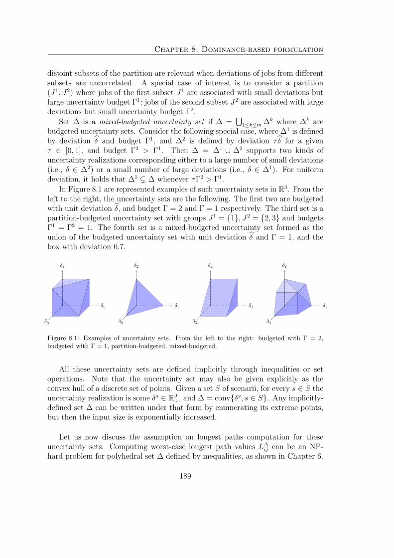
Chapter 8. Dominance-based formulation
disjoint subsets of the partition are relevant when deviations of jobs from differentsubsets are uncorrelated. A special case of interest is to consider a partition(J1, J2) where jobs of the first subset J1 are associated with small deviations butlarge uncertainty budget Γ1; jobs of the second subset J2 are associated with largedeviations but small uncertainty budget Γ2.
Set ∆ is a mixed-budgeted uncertainty set if ∆ =⋃
1≤k≤m ∆k where ∆k arebudgeted uncertainty sets. Consider the following special case, where ∆1 is definedby deviation δ and budget Γ1, and ∆2 is defined by deviation τ δ for a givenτ ∈ [0, 1], and budget Γ2 > Γ1. Then ∆ = ∆1 ∪ ∆2 supports two kinds ofuncertainty realizations corresponding either to a large number of small deviations(i.e., δ ∈ ∆2) or a small number of large deviations (i.e., δ ∈ ∆1). For uniformdeviation, it holds that ∆1 ( ∆ whenever τΓ2 > Γ1.
In Figure 8.1 are represented examples of such uncertainty sets in R3. From theleft to the right, the uncertainty sets are the following. The first two are budgetedwith unit deviation δ, and budget Γ = 2 and Γ = 1 respectively. The third set is apartition-budgeted uncertainty set with groups J1 = {1}, J2 = {2, 3} and budgetsΓ1 = Γ2 = 1. The fourth set is a mixed-budgeted uncertainty set formed as theunion of the budgeted uncertainty set with unit deviation δ and Γ = 1, and thebox with deviation 0.7.
δ1
δ2
δ3
δ1
δ2
δ3
δ1
δ2
δ3
δ1
δ2
δ3
Figure 8.1: Examples of uncertainty sets. From the left to the right: budgeted with Γ = 2,budgeted with Γ = 1, partition-budgeted, mixed-budgeted.
All these uncertainty sets are defined implicitly through inequalities or setoperations. Note that the uncertainty set may also be given explicitly as theconvex hull of a discrete set of points. Given a set S of scenarii, for every s ∈ S theuncertainty realization is some δs ∈ RJ
+, and ∆ = conv{δs, s ∈ S}. Any implicitly-defined set ∆ can be written under that form by enumerating its extreme points,but then the input size is exponentially increased.
Let us now discuss the assumption on longest paths computation for theseuncertainty sets. Computing worst-case longest path values L∆
ij can be an NP-hard problem for polyhedral set ∆ defined by inequalities, as shown in Chapter 6.
189
Chapter 8. Dominance-based formulation
However, efficient algorithms can be designed for some uncertainty sets. Forbox uncertainty, the computation is straightforward since L∆
ij = LG(p+δ)(i, j). Forbudgeted uncertainty sets, and thus 1-disruption uncertainty sets, the worst-caselongest path values L∆
ij can be computed in polynomial time by dynamic program-ming (Minoux, 2009). The algorithm is linear in Γ|A|.
For partition-budgeted uncertainty sets, the L∆ij values can be computed using
a straightforward generalization of the dynamic programming of (Minoux, 2009)which is linear in (Π1≤k≤mΓk)|A|. For mixed-budgeted uncertainty sets, the L∆
ij
values can be easily obtained since L∆ij = max1≤k≤m L
∆k
ij for every i, j ∈ J . Forexplicitly-defined uncertainty sets, values L∆
ij can be computed in polynomial timein the number of scenarii |S|, since L∆
ij = maxs∈S LG(p+δs)(i, j). This relies on the
property that L∆ij = L
conv(∆)ij for any ∆.
For all considered uncertainty sets, the L∆ij values can thus be computed in
polynomial time. In the sequel, we consider the L∆ij values as precomputed in
a preprocessing step. Thus they will appear as coefficients of constraints in theproposed mixed-integer programming formulations.
8.2 Linear formulations for AnchRobPSP
In this section, we establish linear formulations for AnchRobPSP using L∆ij values
as coefficients. A naive formulation is first given as a benchmark. The main dom-inance property is proven, and formulation (Dom) is derived from it. Formulation(Dom) is then compared to other formulations.
8.2.1 A naive formulation
Consider schedule continuous variables xj, j ∈ J , and anchoring binary variableshj ∈ {0, 1}, j ∈ J . Vector h is the incidence vector of the anchored set H.A formulation for AnchRobPSP requires constraints to enforce that H is an x-anchored set. The characterization of Theorem 6.1 suggests a quadratic constraint
xj − xi ≥ L∆ijhihj ∀i, j ∈ J, i ≺ j (1)
to represent precedence constraints of the graph GH . Note that for dummy jobss and t there is no hj decision variable but we set hs = 1 and ht = 0 for the easeof notation. For validity, it is sufficient to check that for each i ≺ j, if hi = 0 orhj = 0 then inequality (1) is valid. Indeed it reduces to xj − xi ≥ 0 which holdsfor every i ≺ j for every schedule x of G(p).
190
Chapter 8. Dominance-based formulation
Applying a standard linearization technique, a linear formulation (Std) can beobtained by replacing constraint (1) by the following linear inequality (2)
(Std): max∑
i∈J wihis.t. xj − xi ≥ pi ∀(i, j) ∈ A
xt ≤Mxj − xi ≥ L∆
ij(hi + hj − 1) ∀i, j ∈ J, i ≺ j (2)
xj ≥ 0 ∀j ∈ Jhj ∈ {0, 1} ∀j ∈ J
It is easy to check that when hi = 0 or hj = 0, (2) induces a valid constraint.
8.2.2 A dominance property
Let X≤M denote the set of schedules of G(p) with makespan at most M . LetH ⊆ J be a subset of jobs. Let us define the set of all baseline schedules x suchthat (x,H) is feasible for AnchRobPSP, i.e., X≤M(H) = {x ∈ X≤M : H is x-anchored}. Note that AnchRobPSP problem is to maximize the weight of a set Hsuch that X≤M(H) 6= ∅. By Theorem 6.1,
X≤M(H) = {x ∈ X≤M : xj − xi ≥ L∆ij ∀i ∈ H ∪ {s}, j ∈ H, i ≺ j}.
Let us now define a set of baseline schedules where the same inequality isimposed, but on pairs i, j with i ∈ J ∪ {s}:
Z≤M(H) = {z ∈ X≤M : zj − zi ≥ L∆ij ∀i ∈ J ∪ {s}, j ∈ H, i ≺ j}.
Theorem 8.1. Set Z≤M(H) is dominant, in the sense that Z≤M(H) ⊆ X≤M(H),and X≤M(H) 6=∅ implies Z≤M(H) 6=∅.
Proof. Since H ⊆ J , the definition of set Z≤M(H) contains more constraints thanthat of set X≤M(H). Hence Z≤M(H) ⊆ X≤M(H). Let us prove X≤M(H) 6=∅ =⇒ Z≤M(H) 6= ∅. Recall that GH is the precedence graph obtained from G(p)by introducing additional arcs (i, j), i ∈ H ∪ {s}, j ∈ H, i ≺ j with arc-lengths
L∆ij . Note that X≤M(H) is exactly the set of schedules of GH with makespan at
most M . Let z be the earliest schedule of GH . By assumption, there exists aschedule in X≤M(H), thus zt ≤ M . Let i ∈ J ∪ {s} and j ∈ H. Let us showthat zj − zi ≥ L∆
ij holds, even for i /∈ H ∪ {s}. Consider a longest s−i path P ∗siin GH , and let k ∈ H ∪ {s} be the last vertex of H ∪ {s} on this path. Thenzi = LGH (s, i) = LGH (s, k) + LGH (k, i) = zk + LGH (k, i). The subpath of P ∗si from
k to i is a longest k−i path in GH . Since it has no vertex in H ∪ {s} except k, ituses no additional arc and its length is LGH (k, i) = L0
ki. It comes zk − zi = −L0ki.
191
Chapter 8. Dominance-based formulation
Since z ∈ X≤M(H), zj− zk ≥ L∆kj. Then zj− zi = (zj− zk) + (zk− zi) ≥ L∆
kj−L0ki.
Also, for k ≺ i ≺ j, it holds that L∆kj ≥ L0
ki + L∆ij : indeed L∆
ij is attained for someδ∗ ∈ ∆ ⊆ RJ
+, hence L∆kj ≥ LG(p+δ∗)(k, i) + LG(p+δ∗)(i, j) ≥ L0
ki + L∆ij . Finally
zj − zi ≥ L∆ij , hence z ∈ Z≤M(H).
8.2.3 Dominance-based linear formulation (Dom)
AnchRobPSP problem is to maximize the weight of a set H such that X≤M(H) 6=∅, or equivalently with Theorem 8.1, such that Z≤M(H) 6= ∅. We now intro-duce a new formulation derived from Theorem 8.1, where continuous variables zcorrespond to a schedule z ∈ Z≤M(H).
(Dom): max∑
i∈J wihis.t. zj − zi ≥ pi ∀(i, j) ∈ A
zt ≤Mzj − zi ≥ L0
ij + (L∆ij − L0
ij)hj ∀i, j ∈ J, i ≺ j (3)
zj ≥ 0 ∀j ∈ Jhj ∈ {0, 1} ∀j ∈ J
Proposition 8.1. Formulation (Dom) is valid for AnchRobPSP.
Proof. Let (z, h) be feasible for (Dom), and H := {i ∈ J : hi = 1}. Note first thatinequality (3) implies z ∈ X≤M(H). Hence z is a schedule with makespan at mostM and H is z-anchored. Hence h ∈ H. Conversely, let h ∈ H be the incidencevector of an anchored set H. From Theorem 8.1, there exists z ∈ Z≤M(H). Sucha schedule z satisfies zj − zi ≥ L∆
ij for every i ∈ J ∪ {s} and j ∈ H. Then zsatisfies (3): indeed if hj = 1 inequality (3) corresponds to inequality zj−zi ≥ L∆
ij ;if hj = 0 then (3) amounts to zj − zi ≥ L0
ij, which holds since z is a schedule ofG(p).
Note that precedence constraint zj − zi ≥ pi associated with arc (i, j) ∈ A isimplied by (3) since i ≺ j and L0
ij ≥ pi.
We now introduce a family of valid inequalities. Let j ∈ J . By inequality (3)with i = s, it comes that zj ≥ L0
sj + (L∆sj − L0
sj)hj. Since z ∈ X≤M it satisfieszj +L0
jt ≤M , thus leading to M ≥ L0sj + (L∆
sj −L0sj)hj +L0
jt. Hence the followingvalid inequality
hj ≤⌊M − (L0
sj + L0jt)
L∆sj − L0
sj
⌋. (4)
In Section 8.3 these inequalities will be discussed with respect to the polyhedralcharacterization under box uncertainty.
192
Chapter 8. Dominance-based formulation
8.2.4 Comparison between (Dom) and other formulations
In this section it is shown that formulation (Dom) is stronger than (Std), andstronger than (Lay) in some cases of interest.
Consider first the continuous relaxations of (Dom), (Std) and the variant of(Std) with quadratic constraint (1). It turns out that they can easily be compared.Indeed for every hi, hj ∈ [0, 1], it holds that hj ≥ hihj. Hence the right-hand sideof inequality (3) is tighter than the right-hand side of inequality (1). Also for everyhi, hj ∈ [0, 1], it holds that (1− hi)(1− hj) ≥ 0 or equivalently hihj ≥ hi + hj − 1.Hence the right-hand side of inequality (1) is tighter than the right-hand side ofinequality (2).
Let us now investigate the special case of budgeted uncertainty, and compare(Dom) with formulation (Lay), that we now recall. Formulation (Lay) involvesanchoring variables hj ∈ {0, 1} for every j ∈ J , and continuous variables xγj for
every γ ∈ {0, . . . ,Γ}, j ∈ J . Formulation (Lay) is based on a so-called layeredgraph Glay(h) associated with h ∈ [0, 1]J and built as follows. The layered graphGlay(h) is formed with Γ + 1 copies of the precedence graph called layers indexedfrom 0 to Γ. Let iγ denote the copy of job i in layer γ. The layered graph featuresthree types of arcs. Horizontal arcs are copies of arcs of G(p), i.e., arcs (iγ, jγ) for(i, j) ∈ A, with length pi. Transversal arcs are (iγ+1, jγ) for (i, j) ∈ A, with length
pi + δi. Vertical arcs are (iγ, iΓ) for i ∈ J , γ < Γ, with length −Dj(1− hj), whereDj is a bigM value. A valid choice is Dj = LG(p+δ)(s, j) − LG(p)(s, j) for every
j ∈ J . It was shown that h ∈ {0, 1}J is the incidence vector of an anchored set ifand only if there exists x a schedule of Glay(h) such that xΓ
t ≤ M , see page 114.This leads to the formulation
(Lay): max∑
i∈J wihis.t. xγj − x
γi ≥ pi ∀(i, j) ∈ A, ∀γ ∈ {0, . . . ,Γ}
xγj − xγ+1i ≥ pi + δi ∀(i, j) ∈ A, ∀γ ∈ {0, . . . ,Γ− 1}
xΓj − x
γj ≥ −Dj(1− hj) ∀j ∈ J , ∀γ ∈ {0, . . . ,Γ− 1}
xΓt ≤Mxγj ≥ 0 ∀j ∈ J, ∀γ ∈ {0, . . . ,Γ}hj ∈ {0, 1} ∀j ∈ J
Variables xΓj , j ∈ J from layer Γ can be interpreted as a baseline schedule such
that H = {i ∈ J : hi = 1} is xΓ-anchored. Other continuous variables xγj , j ∈ J ,γ < Γ can be regarded as additional variables.
Let PLay (resp. PDom) denote the polytope of solutions ((xγ)γ∈{0,...,Γ}, h) (resp.(z, h)) that are feasible for the continuous relaxation of formulation (Lay) (resp.
193
Chapter 8. Dominance-based formulation
(Dom)). Consider the following assumption on the Dj values, denoted by (IneqDj)
for every i ≺ j, Dj ≥ L∆ij − L0
ij. (IneqDj)
Note that assumption (IneqDj) is that Dj values are “large enough”. In formula-tion (Lay) they play the role of bigM values. We set Dj = LG(p+δ)(s, j)−LG(p)(s, j)
because it is a tight value for which (Lay) is valid. The formulation would remainvalid for larger values of Dj’s. In the sequel, we will show that the (IneqDj) as-sumption is satisfied for critical precedence graphs, i.e., precedence graphs whereall s−t paths are longest s−t paths. We now prove
Proposition 8.2. Under assumption (IneqDj), formulation (Dom) is strongerthan formulation (Lay), in the sense that Projh(PDom) ⊆ Projh(PLay).
Proof. Let h ∈ Projh(PDom), i.e., h ∈ [0, 1]J such that there exists a schedulez satisfying inequalities (3) and zt ≤ M . We want to prove the existence of a
schedule x of Glay(h) with makespan xΓt ≤ M . Let us build a graph G as follows:
it contains the graph Glay(0) (no vertical arcs) to which we add precedence arcs(i, j) for i ≺ j with weight L0
ij + (L∆ij −L0
ij)hj in the upper layer, so that to enforce
constraints (3). Let x be the earliest schedule of G. Since G has no vertical arc,
the longest sΓ−tΓ path in G is the longest sΓ−tΓ path in its upper layer. Becauseof the existence of schedule z, the longest sΓ−tΓ path in the upper layer of G haslength at most M .
Let us show that x is a schedule of Glay(h): it is sufficient to show that verticalarcs constraints are satisfied, i.e., that xΓ
j − xγj ≥ −Dj(1 − hj) for every j ∈ J ,
γ ∈ {0, . . . ,Γ}. Let us denote by Lγij the longest i−j path with uncertainty budgetγ (then LΓ
ij = L∆ij). Let j ∈ J , γ ∈ {0, . . . ,Γ}. By definition of x, there exists
i∗ ∈ J ∪ {s} such that
xγj = xΓi∗ + LΓ−γ
i∗j
E.g., this equality is satisfied with i∗ the last vertex in the upper layer on a longestpath from sΓ to jγ. Because of arcs in the upper layer, we also have
xΓj − xΓ
i∗ ≥ L0i∗j + (LΓ
i∗j − L0i∗j)hj.
Combining the two latter (in)equalities, we obtain xΓj−x
γj = (xΓ
j−xΓi∗)+(xΓ
i∗−xγj ) ≥
L0i∗j + (LΓ
i∗j − L0i∗j)hj − LΓ−γ
i∗j = (LΓi∗j − L0
i∗j)hj − (LΓ−γi∗j − L0
i∗j). Let f(hj) =
(LΓi∗j−L0
i∗j)hj−(LΓ−γi∗j −L0
i∗j) denote this latter quantity. Let also g(hj) = −Dj(1−hj). Both are affine functions of hj. The inequality f(hj) ≥ g(hj) writes as
(Dj − LΓi∗j + L0
i∗j)hj ≤ Dj − LΓ−γi∗j + L0
i∗j. The right-hand side can be lower-bounded by Dj − LΓ
i∗j + L0i∗j (attained for γ = 0). By assumption (IneqDj),
Dj − LΓi∗j + L0
i∗j ≥ 0 and the inequality f(hj) ≥ g(hj) holds for every hj ∈ [0, 1]
194
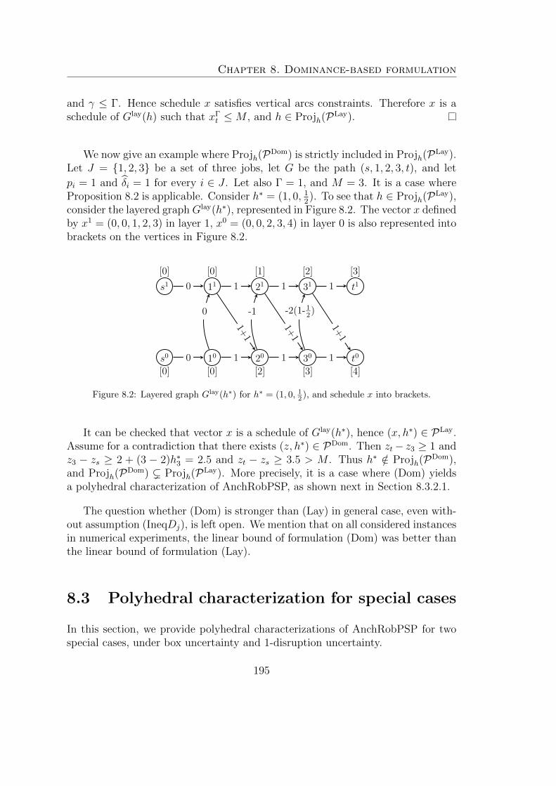
Chapter 8. Dominance-based formulation
and γ ≤ Γ. Hence schedule x satisfies vertical arcs constraints. Therefore x is aschedule of Glay(h) such that xΓ
t ≤M , and h ∈ Projh(PLay).
We now give an example where Projh(PDom) is strictly included in Projh(PLay).Let J = {1, 2, 3} be a set of three jobs, let G be the path (s, 1, 2, 3, t), and let
pi = 1 and δi = 1 for every i ∈ J . Let also Γ = 1, and M = 3. It is a case whereProposition 8.2 is applicable. Consider h∗ = (1, 0, 1
2). To see that h ∈ Projh(PLay),
consider the layered graph Glay(h∗), represented in Figure 8.2. The vector x definedby x1 = (0, 0, 1, 2, 3) in layer 1, x0 = (0, 0, 2, 3, 4) in layer 0 is also represented intobrackets on the vertices in Figure 8.2.
s0 10 20 30 t0
s1 11 21 31 t1
0 1 1 1
0 1 1 1
1+1
1+1
1+1
0 -1 -2(1-12)
[0] [0] [1] [2] [3]
[0] [0] [2] [3] [4]
Figure 8.2: Layered graph Glay(h∗) for h∗ = (1, 0, 12 ), and schedule x into brackets.
It can be checked that vector x is a schedule of Glay(h∗), hence (x, h∗) ∈ PLay.Assume for a contradiction that there exists (z, h∗) ∈ PDom. Then zt− z3 ≥ 1 andz3 − zs ≥ 2 + (3 − 2)h∗3 = 2.5 and zt − zs ≥ 3.5 > M . Thus h∗ /∈ Projh(PDom),and Projh(PDom) ( Projh(PLay). More precisely, it is a case where (Dom) yieldsa polyhedral characterization of AnchRobPSP, as shown next in Section 8.3.2.1.
The question whether (Dom) is stronger than (Lay) in general case, even with-out assumption (IneqDj), is left open. We mention that on all considered instancesin numerical experiments, the linear bound of formulation (Dom) was better thanthe linear bound of formulation (Lay).
8.3 Polyhedral characterization for special cases
In this section, we provide polyhedral characterizations of AnchRobPSP for twospecial cases, under box uncertainty and 1-disruption uncertainty.
195
Chapter 8. Dominance-based formulation
8.3.1 Box uncertainty
This section is devoted to box uncertainty, which is the special case of budgeteduncertainty where Γ = |J |, and thus δ ∈ ∆. In Section 6.4.1 of Chapter 6, apolynomial algorithm for AnchRobPSP under box uncertainty was provided. Thisalgorithm is as follows: compute x the earliest schedule of G(p+ δ) and x the latestschedule of G(p) such that xt = M ; let H∗ = {i ∈ J | xi ≤ xi} and xi = min{xi, xi}for every i ∈ J ; return (x,H∗).
The main result is that in this case the polytope Q of anchored sets is charac-terized by inequalities (4).
Theorem 8.2. For box uncertainty,
Q = {h ∈ [0, 1]J : h satisfies (4)}.
Proof. Consider schedules x and x, defined by xj = LG(p+δ)(s, j) and xj = M−L0jt
for every j ∈ J . Note first that for box uncertainty, L∆sj = LG(p+δ)(s, j) = xj. In-
equality (4) writes in this case: hj ≤⌊M−(L0
sj+L0jt)
L∆sj−L0
sj
⌋=⌊xj−L0
sj
xj−L0sj
⌋. Equivalently,
it implies hj ≤ 1 if j ∈ H∗, and hj ≤ 0 if j /∈ H∗. Hence {h ∈ [0, 1]J :h satisfies (4)} = [0, 1]H
∗ × {0}J\H∗ .Every extreme point of [0, 1]H
∗ × {0}J\H∗ is the incidence vector of a set H ⊆H∗. Since any subset of an anchored set is anchored, and H∗ is anchored, then[0, 1]H
∗×{0}J\H∗ ⊆ Q. Conversely, if H is an anchored set, its incidence vector χH
satisfies valid inequalities (4): thus H ⊆ H∗. Hence Q ⊆ [0, 1]H∗ × {0}J\H∗ .
Note that Theorem 8.2 also holds for any ∆ that has a greatest element δ. Thiscase is more general than ∆ being a box, as mentioned in Section 8.1.
8.3.2 1-disruption uncertainty
In this section, set ∆ is a 1-disruption uncertainty set, i.e., a budgeted uncertaintyset with Γ = 1 and δi = δ0 for every i ∈ J . In Section 8.3.2.1 the polyhedralcharacterization is shown for the special case with processing times equal to zero.In Section 8.3.2.2 it is extended to any critical precedence graph, with possiblynon-zero processing times.
8.3.2.1 The Unitary AnchRobPSP
Consider first the case of zero processing times. W.l.o.g. δ0 = 1. This is theUnitary AnchRobPSP (U-AnchRob) studied in Section 6.4.2.2, page 124. For unit
196
Chapter 8. Dominance-based formulation
anchoring weights, it was identified as a polynomial case by an equivalence with aproblem on posets for which a min/max theorem is known (Schrijver, 2003).
An instance is the precedence graph G = (J,A), p = 0, δ0 = 1, integer deadlineM , and anchoring weights. Indeed deadline M can be assumed integer. If M isnot integer, it can be replaced with bMc w.l.o.g.: indeed, since p and δ are integer,for any H the earliest schedule of for which H is anchored is integer-valued withinteger makespan.
For (U-AnchRob) our main result is a characterization of the polytope throughformulation (Dom). It relies on the polyhedral result of Theorem 8.3. Let (J,≺) bea poset with s (resp. t) a least (resp. greatest) element. Consider the inequalities
zi − zs ≥ 0 ∀i ∈ J (a)zt − zi ≥ 0 ∀i ∈ J (b)zt ≤M (c)zj − zi ≥ hj ∀i, j ∈ J , i ≺ j (d)zj ≥ 0 ∀j ∈ J (e)hj ≤ 1 ∀j ∈ J (f)hj ≥ 0 ∀j ∈ J (g)
and let P = {(z, h) ∈ RJ × RJ : (a)− (g)}.
Theorem 8.3. The polytope P is integer.
Proof. Consider the polytope P formed with all pairs (z, h) ∈ RJ+ ×RJ
+ satisfyingthe constraints (a)–(g). To prove integrality of P , the main idea is to define anauxiliary extended polyhedron where h variables can be expressed linearly fromz variables and additional z′ variables. Let us define the auxiliary polyhedron P ′formed with all triplets (z, z′, h) ∈ RJ
+ × RJ+ × RJ satisfying the constraints
zj − zi ≥ 0 ∀(i, j) ∈ A (i)z′j − z′i ≥ 0 ∀(i, j) ∈ A (ii)z′j − zi ≥ 1 ∀(i, j) ∈ A (iii)zj − z′j ≥ −1 ∀j ∈ J (iv)zj − z′j ≤ 0 ∀j ∈ J (v)zt ≤M (vi)hj = 1 + zj − z′j ∀j ∈ J (vii)
Let us prove the following claim. Claim 1. P = Projz,h(P ′).First, given (z, h) ∈ P , let us prove the existence of z′ such that (z, z′, h) ∈ P ′.Define z′j = 1 + zj − hj for every j ∈ J , and z′s = zs, z
′t = 1 + zt. Then the
(in)equalities (i) to (vii) can be checked for the triplet (z, z′, h) as follows.– (i) and (vi) hold by assumption on z, and (vii) by definition of z′;
197
Chapter 8. Dominance-based formulation
– (ii): if j 6= t then z′j − z′i = zj − zi − hj + hi ≥ hi ≥ 0 by (d); if j = t thenz′j − z′i = zt − zi + hi ≥ hi ≥ 0 by (b);
– (iii): if j 6= t then z′j − zi = 1 + zj − hj − zi ≥ 1 by (d); if j = t, followsfrom (b);
– (iv) and (v): zj − z′j = −1 + hj ∈ [−1, 0] since hj ∈ [0, 1].Conversely, let (z, z′, h) ∈ P ′. Let us check inequalities (a)–(g) for (z, h).
– (a) holds by sum of (i) along an s−i path;– (b) holds by sum of (i) along an i−t path;– (c) is clear;– (d): for i ≺ j we have zj − zi = zj − z′j + z′j − zk + zk − zi, where k is the
last vertex distinct from j on a path from i to j in the precedence graph(possibly k = i). Then (k, j) ∈ A so z′j − zk ≥ 1 by (iii). Also zk − zi ≥ 0 bysumming (i) along the i−k path. Hence zj − zi ≥ zj − z′j + 1 + 0 = hj by(vii). Hence (d) is satisfied;
– (f) (resp. (g)) comes from (vii) and (iv) (resp. (vii) and (v)).This completes the proof of Claim 1. �
Now we prove: Claim 2. P ′ is integer.Let (z, z′, h) be an extreme point of P ′. It satisfies the n equalities (vii) and itsaturates 2(n + 2) linearly independent inequalities among (i)–(vi). Thus (z, z′)
is an extreme point of {(z, z′) ∈ RJ+ × RJ
+ : (i)-(vi)}. The constraint matrix of(i)–(vi) is totally unimodular, and the right-hand side is integer since M is integer.Hence (z, z′) is integer and so is (z, z′, h). This ends the proof of Claim 2. �
By Claim 1, P = Projz,h(P ′). It holds that for any extreme point (z, h) ofP there exists z′ such that (z, z′, h) is an extreme point of P ′. By Claim 2, such(z, z′, h) is integer, hence (z, h) is integer. This proves the integrality of P .
Theorem 8.3 implies the following polyhedral characterization
Proposition 8.3. Formulation (Dom) yields a polyhedral characterization for (U-AnchRob).
Proof. Let us prove that the linear relaxation of (Dom) correponds to the polytopeP from Theorem 8.3. For (U-AnchRob) for every i, j ∈ J such that i ≺ j we haveL0ij = 0 since p = 0. The worst-case longest paths values are as follows. For every
j ∈ J , L∆sj = 0 if j has no predecessor except s, and L∆
sj = 1 otherwise. For everyi ≺ j with i 6= s, L∆
ij = 1. For a pair i ≺ j with i 6= s, inequality (3) thus writeszj − zi ≥ hj, which is inequality (d) or (b) from the definition of P . For a pairs ≺ j, inequality (3) writes zj−zs ≥ 0 if j has no predecessor in J , and zj−zs ≥ hjotherwise. If j has no predecessor in J , it is inequality (a) from the definition ofP . Otherwise j has a predecessor k ∈ J and inequality zj − zs ≥ hj is dominatedby inequalities zk − zs ≥ 0 and zj − zk ≥ hk. Hence it is satisfied by any elementof P . Thus PDom = P .
198
Chapter 8. Dominance-based formulation
By Theorem 8.3, P is integer, hence Projh(P) is integer. Namely, each extremepoint of Projh(P) is the incidence vector of an anchored set. Thus Projh(PDom) =Projh(P) = Q, and (Dom) yields a polyhedral characterization for the problem.
Note that Proposition 8.3 implies also the integrality of schedule variables z,which are not required to be integer in general.
As a corollary, a complexity result is that Theorem 8.3 generalizes the polyno-mial case of (U-AnchRob) proven in Chapter 6 for unit anchoring weights, to anynon-negative anchoring weights.
8.3.2.2 Critical precedence graphs
Let us now consider processing times p ∈ RJ+ and consider the case of critical
precedence graphs. Recall that the precedence graph G(p) is critical if the lengthof all s−t paths is the same.
Properties of critical precedence graphs. A case where G(p) is critical iswhen processing times are equal to zero, since the length of all s−t paths is zero.Also if G is a path, for any p the precedence graph G(p) is critical since there isa unique s−t path. Let us say that the precedence graph G(p) is quasi-criticalif every job i ∈ J belongs to a critical path, i.e., L0
si + L0it = L0
st. Note thatif G(p) is critical, a necessary condition is that it is quasi-critical. For non-zeroprocessing times, it can also be proven that for some precedence graphs, if G(p) isquasi-critical then it is critical. This holds for series-parallel precedence graphs.
Proposition 8.4. If G is series-parallel and G(p) is quasi-critical, then G(p) iscritical.
Proof. If G is a path, then G(p) is critical. If G is obtained by series compositionof G1 and G2; then any s−t path is formed by an s1−t1 path in G1 and ans2−t2 path in G2. Hence if G1 and G2 are critical, it follows that G is critical.If G is obtained by parallel composition of G1 and G2, both critical, let i ∈ G1
and j ∈ G2. Then every s−t path going through G1 (resp. G2) has lengthLG1(s, t) = LG1(s, i) + LG1(i, t) (resp. LG2(s, t) = LG2(s, j) + LG2(j, t)). If G isquasi-critical, LG(s, i) + LG(i, t) = LG(s, j) + LG(j, t), and it follows that all s−tpaths of G have same length.
This result is used for numerical results in Section 8.4 to generate criticalprecedence graphs.
199
Chapter 8. Dominance-based formulation
Let us now show
Proposition 8.5. If G(p) is critical, then the assumption (IneqDj) is satisfied forvalues Dj = LG(p+δ)(s, j)− LG(p)(s, j), for any uncertainty set ∆ ⊆ RJ
+.
Proof. Let i ≺ j. By definition of Dj, it holds that Dj ≥ L∆sj − L0
sj. BecauseG(p) is critical, it holds that L0
sj = L0si + L0
ij. Hence Dj ≥ L∆sj − L0
si − L0ij. By
definition of the L∆ij values, it holds that L∆
sj ≥ L0si +L∆
ij . Hence Dj ≥ L∆ij −L0
ij asclaimed.
Hence by Proposition 8.2, for critical precedence graphs, formulation (Dom) isstronger than formulation (Lay).
Polyhedral characterization for critical precedence graphs. Let us nowconsider a critical precedence graph G(p), and extend the polyhedral characteri-
zation result obtained in Section 8.3.2.1. It is assumed that M = L0st + δ0M
′ with
M ′ integer. Indeed M can be tightened to L0st + δ0
⌊(M − L0
st)/δ0
⌋w.l.o.g. Under
this assumption we prove that
Theorem 8.4. For 1-disruption uncertainty and critical precedence graph,formulation (Dom) yields a polyhedral characterization of AnchRobPSP.
Proof. Let I denote an instance of AnchRobPSP for 1-disruption uncertainty withdeviation δ0, critical precedence graph G(p), and deadline M . Let z∗ be the earliestschedule of G(p), namely z∗i = L0
si for every i ∈ J . Since G(p) is critical, for everyi ≺ j it holds that L0
si + L0ij + L0
jt = L0sj + L0
jt, hence L0ij = z∗j − z∗i . Also
L∆ij = z∗j − z∗i + δ0. Inequalities (3) then write zj − zi ≥ (z∗j − z∗i ) + δ0hj, or
equivalentlyzj−z∗jδ0− zi−z∗i
δ0≥ hj. Similarly the deadline constraint is equivalent
tozt−z∗tδ0≤ M−z∗t
δ0. Consider a new instance I ′ of (U-AnchRob) defined by: the
precedence graph G, zero processing times, and M ′ =M−L0
st
δ0. Then M ′ is integer
by assumption on M . Solution (z, h) is feasible for (Dom) in instance I if andonly if solution ( z−z
∗
δ0, h) is feasible for (Dom) in instance I ′. Hence if (z, h) is an
extreme point of PDom then ( z−z∗
δ0, h) is extreme for the (U-AnchRob) instance.
By Proposition 8.3, vector h is integer. Hence the claimed result.
Theorem 8.4 thus yields a polyhedral characterization of polynomial size forthis special case. We mention that this is a polynomial case of AnchRobPSP thatwas not identified in Chapter 6.
200
Chapter 8. Dominance-based formulation
8.4 Numerical results
We investigate the impact of theoretical polyhedral results from Section 8.3 on theperformance of formulations (Lay), (Std), (Dom) for various instance classes. InSection 8.4.1, instances and settings are presented. Section 8.4.2 is dedicated tobudgeted uncertainty, and Section 8.4.3 to partition-budgeted and mixed-budgeteduncertainty sets.
8.4.1 Instances and settings
Instances are randomly generated as follows. We consider instance classes with afour-field label F1 F2 F3 F4:
• Field F1 concerns precedence graph G– ER: precedence graphs randomly generated according to Erdos-Renyi
model, i.e., arc (i, j) is in G with probability pr = 10/n.– SP: Series-Parallel precedence graphs, inductively generated by drawing
randomly series or parallel compositions.• Field F2 denotes processing times p
– pZero: pi = 0 for every i ∈ J ;– pRand: pi is randomly generated in range [5, 20];– pQCri: p is obtained by applying the following procedure: start from
the values generated for class pRand; increase the processing time of arandomly selected job until every job is on a critical path. Hence G(p)is quasi-critical.
• Field F3 denotes deviation δ– dRand: for instances pRand and pQCri, δi is randomly generated in
[1, 12pi] for every i ∈ J ; for instances pZero, δ is equal to the values
generated for instances pQCri;– dUnif: δi = δ0 for every i ∈ J . Value δ0 is randomly selected in the
deviation values of instances dRand.• Field F4 denotes the uncertainty set
– Γ1, Γ2, Γ3 correspond to budgeted uncertainty with deviation definedby F3 and Γ = 1, 2, 3 respectively.
– Partition: jobs are partitioned into two subsets J1 and J2, every jobbeing in J1 with probability 0.75. Given the deviation δ defined byF3, the deviation vector of the Partition instance is b0.1δic for every
i ∈ J1, and δi for every i ∈ J2. Budgets are Γ1 = 10 and Γ2 = 1.– Mixed: ∆ = ∆1 ∪ ∆2 where ∆1 has deviation δ defined by F3 and
Γ1 = 1, and ∆2 has deviation τ δ, with τ = 0.2 and δ defined by F3 andΓ2 = 10.
201
Chapter 8. Dominance-based formulation
Each label corresponds to a class of 10 instances.
By Proposition 8.4 classes SP pQCri yield critical precedence graphs. Note alsothat classes ER pRand (resp. ER pQcri) are generated with the same generationscheme as instances ER (resp. ERC) from Chapter 6.
The number of jobs is set to n = 300. Anchoring weights are unitary. DeadlineM is set to M
12 = 1
2(LG(p)(s, t) + LG(p+δ)(s, t)), that is, it is halfway between the
min makespan of any schedule of G(p) and the min makespan of a robust-static
schedule. Unreported results showed that choosing a deadline other than M12
leads to similar results in terms of the comparison of formulations. For budgeteduncertainty, the budget is Γ ∈ {1, 2, 3}. The choice of a small uncertainty budgetwas previously motivated in the literature, see, e.g., (Herroelen and Leus, 2004),and in the numerical results of Chapter 6.
For each instance, formulations (Dom), (Std), and (Lay) have been imple-mented using Julia 0.6.2, JuMP 0.18.5. Mixed-integer programs are solved withCPLEX 12.8 on a PC under Windows 10 with Intel Core i7-7500U CPU 2.90GHzand 8 Go RAM. The time limit is 300 seconds.
The valid inequalities (4) appear to be added by CPLEX on the fly. Thus theyare not hardcoded in formulations.
8.4.2 Impact of instance parameters under budgeteduncertainty
Let us first investigate the case of budgeted uncertainty. Table 8.1 and Table 8.2present the results for ER and SP instances respectively. Each table presents theresults relative to 8 instance classes: the first 6 instance classes are with Γ = 1 andwith all combinations of processing times and deviations, and the last 2 instanceclasses are with Γ = 2 and Γ = 3. For each instance class, checkmarks in the firstthree columns indicate if the assumptions of Theorem 8.4 are matched:
– crit.: the precedence graph G(p) is critical;
– unif.: deviation δ is uniform;– Γ1: Γ = 1.
The tables feature:
202
Chapter 8. Dominance-based formulation
– opt: average optimal value for instances solved optimally;– for each formulation (Lay), (Std) and (Dom):
– #solved: number of instances, out of 10, solved optimally within thetime limit;
– gap: average final gap of unsolved instances;– time: average computation time for solved instances in seconds;
– LPGap: average gap b−optopt
between integer optimum opt and linearbound b;
– CPXGap: average gap obtained by CPLEX at root node.
The computation times do not include the preprocessing time for computingL∆ij values. The computation is done by a dynamic programming algorithm linear
in Γ|A|. Its running time is negligible with respect to MIP computation time: onaverage 0.153 seconds for ER instances and 0.161 seconds for SP instances.
Let us now comment on the impact of the instance parameters.
Polyhedral characterization cases. Instance classes ER pZero dUnif Γ1, SP -
pZero dUnif Γ1, and SP pQCri dUnif Γ1, correspond to polyhedral characteri-zation cases. As expected, formulation (Dom) solves the problem in less than onesecond and LPGap = 0%. Formulation (Lay) has non-zero LPGap, but CPLEXadds suitable cuts to close the gap at root node.
Impact of uniform deviation. Consider now the 6 instance classes F1 F2 -
dUnif Γ1. These are the first three row entries of Table 8.1 and the first threerow entries of Table 8.2. On these 6 instance classes, formulations (Dom) and(Lay) still behave well. (Dom) solves all instances in less than one second. Inparticular, its LPGap is still very small: at most 0.42%. (Lay) also performs well,the LPGap of (Lay) is larger, but CPXGap is comparable for (Dom) and (Lay).We note that uniform deviation has an important impact on the performance offormulations. Consider, e.g., instance classes SP pZero dUnif Γ1 and SP pZero -
dRand Γ1. For uniform deviation (Dom) is integer ; for non-uniform deviation ithas 9.70% CPXGap and solves only 4 instances out of 10 within the time limit.By contrast with (Dom) and (Lay) on these instances, formulation (Std) performsvery poorly and solves only 41 instances out of 120 (vs. 107 out of 120 for (Dom)).
Impact of the precedence graph. The impact of the precedence graph beingcritical is limited, as shown for example by the comparison of instances ER pZero
and ER pQCri. Both are efficiently solved, while the precedence graph is criticalfor the former, and not critical for the latter. Even more, instances with pRand
appear to be easy instances, while they do not have critical precedence graphs. Aninterpretation is that for such instances, a large number of jobs are not on critical
203
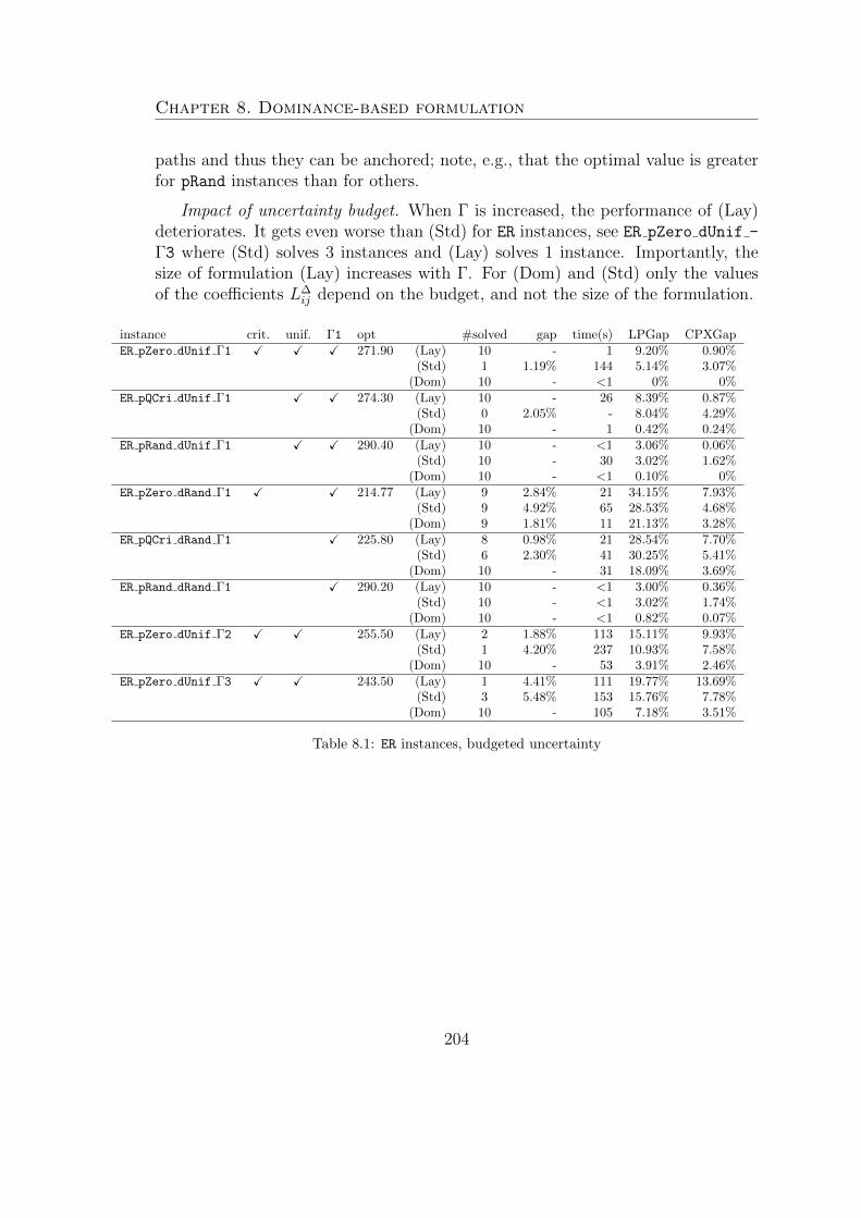
Chapter 8. Dominance-based formulation
paths and thus they can be anchored; note, e.g., that the optimal value is greaterfor pRand instances than for others.
Impact of uncertainty budget. When Γ is increased, the performance of (Lay)deteriorates. It gets even worse than (Std) for ER instances, see ER pZero dUnif -
Γ3 where (Std) solves 3 instances and (Lay) solves 1 instance. Importantly, thesize of formulation (Lay) increases with Γ. For (Dom) and (Std) only the valuesof the coefficients L∆
ij depend on the budget, and not the size of the formulation.
instance crit. unif. Γ1 opt #solved gap time(s) LPGap CPXGapER pZero dUnif Γ1 X X X 271.90 (Lay) 10 - 1 9.20% 0.90%
(Std) 1 1.19% 144 5.14% 3.07%(Dom) 10 - <1 0% 0%
ER pQCri dUnif Γ1 X X 274.30 (Lay) 10 - 26 8.39% 0.87%(Std) 0 2.05% - 8.04% 4.29%
(Dom) 10 - 1 0.42% 0.24%ER pRand dUnif Γ1 X X 290.40 (Lay) 10 - <1 3.06% 0.06%
(Std) 10 - 30 3.02% 1.62%(Dom) 10 - <1 0.10% 0%
ER pZero dRand Γ1 X X 214.77 (Lay) 9 2.84% 21 34.15% 7.93%(Std) 9 4.92% 65 28.53% 4.68%
(Dom) 9 1.81% 11 21.13% 3.28%ER pQCri dRand Γ1 X 225.80 (Lay) 8 0.98% 21 28.54% 7.70%
(Std) 6 2.30% 41 30.25% 5.41%(Dom) 10 - 31 18.09% 3.69%
ER pRand dRand Γ1 X 290.20 (Lay) 10 - <1 3.00% 0.36%(Std) 10 - <1 3.02% 1.74%
(Dom) 10 - <1 0.82% 0.07%ER pZero dUnif Γ2 X X 255.50 (Lay) 2 1.88% 113 15.11% 9.93%
(Std) 1 4.20% 237 10.93% 7.58%(Dom) 10 - 53 3.91% 2.46%
ER pZero dUnif Γ3 X X 243.50 (Lay) 1 4.41% 111 19.77% 13.69%(Std) 3 5.48% 153 15.76% 7.78%
(Dom) 10 - 105 7.18% 3.51%
Table 8.1: ER instances, budgeted uncertainty
204
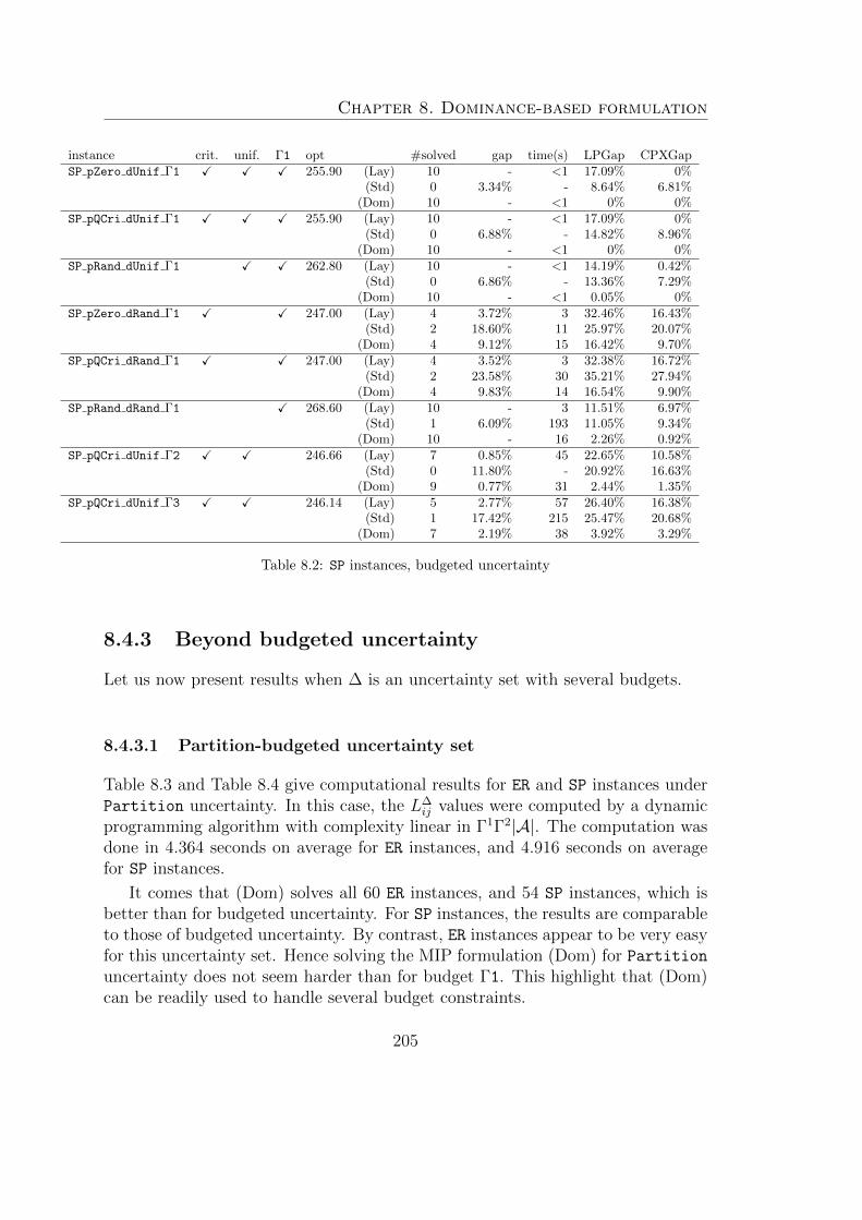
Chapter 8. Dominance-based formulation
instance crit. unif. Γ1 opt #solved gap time(s) LPGap CPXGapSP pZero dUnif Γ1 X X X 255.90 (Lay) 10 - <1 17.09% 0%
(Std) 0 3.34% - 8.64% 6.81%(Dom) 10 - <1 0% 0%
SP pQCri dUnif Γ1 X X X 255.90 (Lay) 10 - <1 17.09% 0%(Std) 0 6.88% - 14.82% 8.96%
(Dom) 10 - <1 0% 0%SP pRand dUnif Γ1 X X 262.80 (Lay) 10 - <1 14.19% 0.42%
(Std) 0 6.86% - 13.36% 7.29%(Dom) 10 - <1 0.05% 0%
SP pZero dRand Γ1 X X 247.00 (Lay) 4 3.72% 3 32.46% 16.43%(Std) 2 18.60% 11 25.97% 20.07%
(Dom) 4 9.12% 15 16.42% 9.70%SP pQCri dRand Γ1 X X 247.00 (Lay) 4 3.52% 3 32.38% 16.72%
(Std) 2 23.58% 30 35.21% 27.94%(Dom) 4 9.83% 14 16.54% 9.90%
SP pRand dRand Γ1 X 268.60 (Lay) 10 - 3 11.51% 6.97%(Std) 1 6.09% 193 11.05% 9.34%
(Dom) 10 - 16 2.26% 0.92%SP pQCri dUnif Γ2 X X 246.66 (Lay) 7 0.85% 45 22.65% 10.58%
(Std) 0 11.80% - 20.92% 16.63%(Dom) 9 0.77% 31 2.44% 1.35%
SP pQCri dUnif Γ3 X X 246.14 (Lay) 5 2.77% 57 26.40% 16.38%(Std) 1 17.42% 215 25.47% 20.68%
(Dom) 7 2.19% 38 3.92% 3.29%
Table 8.2: SP instances, budgeted uncertainty
8.4.3 Beyond budgeted uncertainty
Let us now present results when ∆ is an uncertainty set with several budgets.
8.4.3.1 Partition-budgeted uncertainty set
Table 8.3 and Table 8.4 give computational results for ER and SP instances underPartition uncertainty. In this case, the L∆
ij values were computed by a dynamicprogramming algorithm with complexity linear in Γ1Γ2|A|. The computation wasdone in 4.364 seconds on average for ER instances, and 4.916 seconds on averagefor SP instances.
It comes that (Dom) solves all 60 ER instances, and 54 SP instances, which isbetter than for budgeted uncertainty. For SP instances, the results are comparableto those of budgeted uncertainty. By contrast, ER instances appear to be very easyfor this uncertainty set. Hence solving the MIP formulation (Dom) for Partitionuncertainty does not seem harder than for budget Γ1. This highlight that (Dom)can be readily used to handle several budget constraints.
205
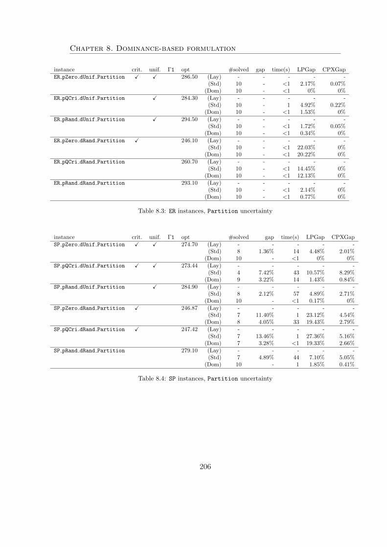
Chapter 8. Dominance-based formulation
instance crit. unif. Γ1 opt #solved gap time(s) LPGap CPXGapER pZero dUnif Partition X X 286.50 (Lay) - - - - -
(Std) 10 - <1 2.17% 0.07%(Dom) 10 - <1 0% 0%
ER pQCri dUnif Partition X 284.30 (Lay) - - - - -(Std) 10 - 1 4.92% 0.22%
(Dom) 10 - <1 1.53% 0%ER pRand dUnif Partition X 294.50 (Lay) - - - - -
(Std) 10 - <1 1.72% 0.05%(Dom) 10 - <1 0.34% 0%
ER pZero dRand Partition X 246.10 (Lay) - - - - -(Std) 10 - <1 22.03% 0%
(Dom) 10 - <1 20.22% 0%ER pQCri dRand Partition 260.70 (Lay) - - - - -
(Std) 10 - <1 14.45% 0%(Dom) 10 - <1 12.13% 0%
ER pRand dRand Partition 293.10 (Lay) - - - - -(Std) 10 - <1 2.14% 0%
(Dom) 10 - <1 0.77% 0%
Table 8.3: ER instances, Partition uncertainty
instance crit. unif. Γ1 opt #solved gap time(s) LPGap CPXGapSP pZero dUnif Partition X X 274.70 (Lay) - - - - -
(Std) 8 1.36% 14 4.48% 2.01%(Dom) 10 - <1 0% 0%
SP pQCri dUnif Partition X X 273.44 (Lay) - - - - -(Std) 4 7.42% 43 10.57% 8.29%
(Dom) 9 3.22% 14 1.43% 0.84%SP pRand dUnif Partition X 284.90 (Lay) - - - - -
(Std) 8 2.12% 57 4.89% 2.71%(Dom) 10 - <1 0.17% 0%
SP pZero dRand Partition X 246.87 (Lay) - - - - -(Std) 7 11.40% 1 23.12% 4.54%
(Dom) 8 4.05% 33 19.43% 2.79%SP pQCri dRand Partition X 247.42 (Lay) - - - - -
(Std) 7 13.46% 1 27.36% 5.16%(Dom) 7 3.28% <1 19.33% 2.66%
SP pRand dRand Partition 279.10 (Lay) - - - - -(Std) 7 4.89% 44 7.10% 5.05%
(Dom) 10 - 1 1.85% 0.41%
Table 8.4: SP instances, Partition uncertainty
206
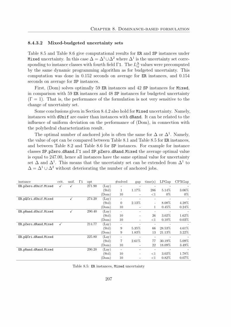
Chapter 8. Dominance-based formulation
8.4.3.2 Mixed-budgeted uncertainty sets
Table 8.5 and Table 8.6 give computational results for ER and SP instances underMixed uncertainty. In this case ∆ = ∆1∪∆2 where ∆1 is the uncertainty set corre-sponding to instance classes with fourth field Γ1. The L∆
ij values were precomputedby the same dynamic programming algorithm as for budgeted uncertainty. Thiscomputation was done in 0.152 seconds on average for ER instances, and 0.154seconds on average for SP instances.
First, (Dom) solves optimally 59 ER instances and 42 SP instances for Mixed,in comparison with 59 ER instances and 48 SP instances for budgeted uncertainty(Γ = 1). That is, the performance of the formulation is not very sensitive to thechange of uncertainty set.
Some conclusions given in Section 8.4.2 also hold for Mixed uncertainty. Namely,instances with dUnif are easier than instances with dRand. It can be related to theinfluence of uniform deviation on the performance of (Dom), in connection withthe polyhedral characterization result.
The optimal number of anchored jobs is often the same for ∆ or ∆1. Namely,the value of opt can be compared between Table 8.1 and Table 8.5 for ER instances,and between Table 8.2 and Table 8.6 for SP instances. For example for instanceclasses SP pZero dRand Γ1 and SP pZero dRand Mixed the average optimal valueis equal to 247.00, hence all instances have the same optimal value for uncertaintyset ∆ and ∆1. This means that the uncertainty set can be extended from ∆1 to∆ = ∆1 ∪∆2 without deteriorating the number of anchored jobs.
instance crit. unif. Γ1 opt #solved gap time(s) LPGap CPXGapER pZero dUnif Mixed X X 271.90 (Lay) - - - - -
(Std) 1 1.17% 286 5.14% 3.06%(Dom) 10 - <1 0% 0%
ER pQCri dUnif Mixed X 274.20 (Lay) - - - - -(Std) 0 2.13% - 8.08% 4.28%
(Dom) 10 - 1 0.45% 0.24%ER pRand dUnif Mixed X 290.40 (Lay) - - - - -
(Std) 10 - 26 3.02% 1.62%(Dom) 10 - <1 0.10% 0.03%
ER pZero dRand Mixed X 214.77 (Lay) - - - - -(Std) 9 5.35% 66 28.53% 4.61%
(Dom) 9 1.83% 13 21.13% 3.22%ER pQCri dRand Mixed 225.80 (Lay) - - - - -
(Std) 7 2.61% 77 30.19% 5.09%(Dom) 10 - 22 18.09% 3.49%
ER pRand dRand Mixed 290.20 (Lay) - - - - -(Std) 10 - <1 3.02% 1.78%
(Dom) 10 - <1 0.82% 0.07%
Table 8.5: ER instances, Mixed uncertainty
207
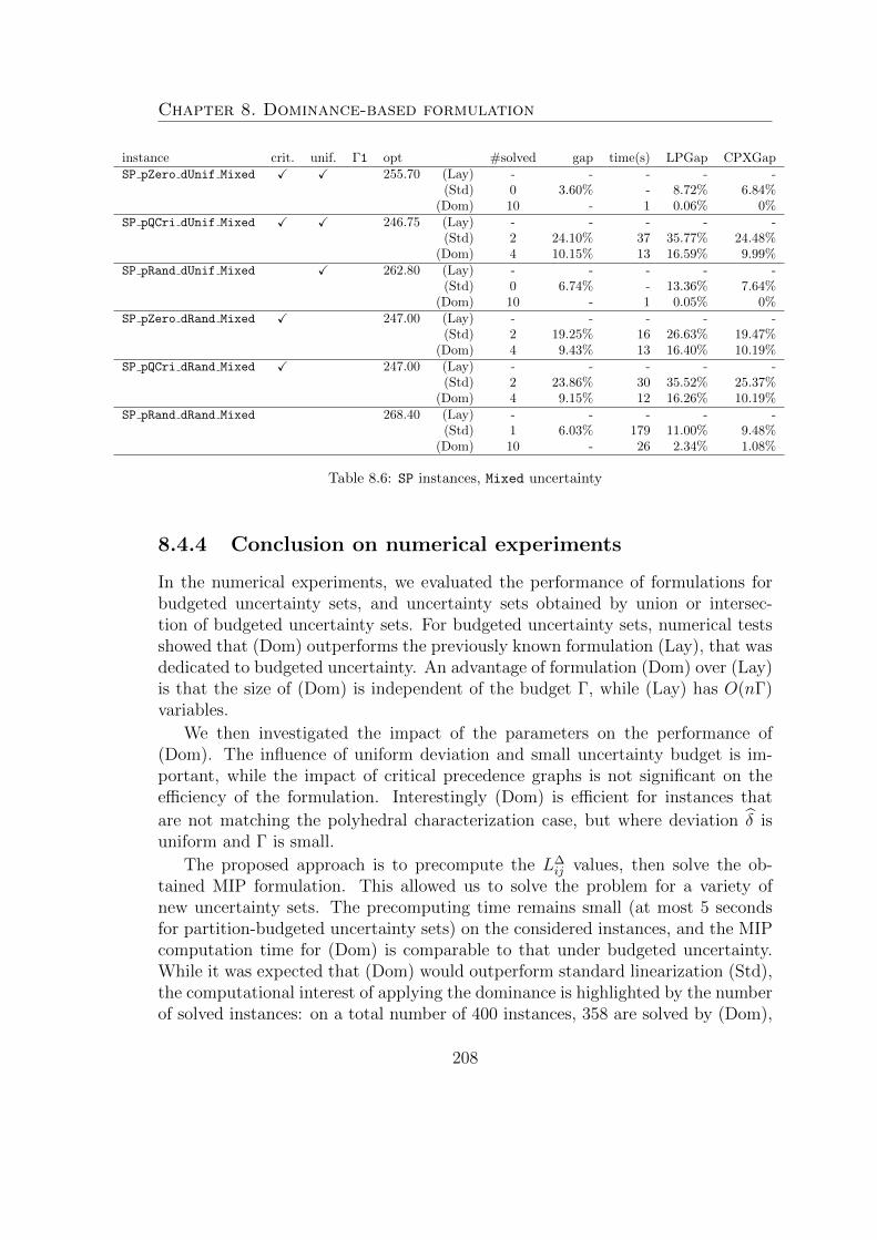
Chapter 8. Dominance-based formulation
instance crit. unif. Γ1 opt #solved gap time(s) LPGap CPXGapSP pZero dUnif Mixed X X 255.70 (Lay) - - - - -
(Std) 0 3.60% - 8.72% 6.84%(Dom) 10 - 1 0.06% 0%
SP pQCri dUnif Mixed X X 246.75 (Lay) - - - - -(Std) 2 24.10% 37 35.77% 24.48%
(Dom) 4 10.15% 13 16.59% 9.99%SP pRand dUnif Mixed X 262.80 (Lay) - - - - -
(Std) 0 6.74% - 13.36% 7.64%(Dom) 10 - 1 0.05% 0%
SP pZero dRand Mixed X 247.00 (Lay) - - - - -(Std) 2 19.25% 16 26.63% 19.47%
(Dom) 4 9.43% 13 16.40% 10.19%SP pQCri dRand Mixed X 247.00 (Lay) - - - - -
(Std) 2 23.86% 30 35.52% 25.37%(Dom) 4 9.15% 12 16.26% 10.19%
SP pRand dRand Mixed 268.40 (Lay) - - - - -(Std) 1 6.03% 179 11.00% 9.48%
(Dom) 10 - 26 2.34% 1.08%
Table 8.6: SP instances, Mixed uncertainty
8.4.4 Conclusion on numerical experiments
In the numerical experiments, we evaluated the performance of formulations forbudgeted uncertainty sets, and uncertainty sets obtained by union or intersec-tion of budgeted uncertainty sets. For budgeted uncertainty sets, numerical testsshowed that (Dom) outperforms the previously known formulation (Lay), that wasdedicated to budgeted uncertainty. An advantage of formulation (Dom) over (Lay)is that the size of (Dom) is independent of the budget Γ, while (Lay) has O(nΓ)variables.
We then investigated the impact of the parameters on the performance of(Dom). The influence of uniform deviation and small uncertainty budget is im-portant, while the impact of critical precedence graphs is not significant on theefficiency of the formulation. Interestingly (Dom) is efficient for instances that
are not matching the polyhedral characterization case, but where deviation δ isuniform and Γ is small.
The proposed approach is to precompute the L∆ij values, then solve the ob-
tained MIP formulation. This allowed us to solve the problem for a variety ofnew uncertainty sets. The precomputing time remains small (at most 5 secondsfor partition-budgeted uncertainty sets) on the considered instances, and the MIPcomputation time for (Dom) is comparable to that under budgeted uncertainty.While it was expected that (Dom) would outperform standard linearization (Std),the computational interest of applying the dominance is highlighted by the numberof solved instances: on a total number of 400 instances, 358 are solved by (Dom),
208
Chapter 8. Dominance-based formulation
only 191 by (Std).
Conclusion
In this chapter we investigated a versatile mixed-integer programming approachfor the AnchRobPSP problem. This led to a linear formulation that is applicableto any uncertainty set, provided that an algorithm for precomputing the worst-case longest paths values is available. This widens the range of uncertainty setsfor which MIP formulations for AnchRobPSP are known. The keypoint for estab-lishing a strong MIP formulation is the analysis of the combinatorial propertiesof AnchRobPSP, among which a dominance property played a major role. Thisproperty allows for a characterization of the anchored sets polytope in interestingspecial cases. The theoretical positive results for the dominance-based formulationalso go together with good numerical performances around the polyhedral char-acterization case, for both budgeted uncertainty and uncertainty sets with severalbudgets.
A research direction would be to apply the same dominance idea to the Anchor-Robust RCPSP studied in Chapter 7. Inequalities could be obtained, to strengthenthe formulation based on the layered graph. This would require to combine theL∆ij computation with the sequence variables. It is worth investigating whether
dominance may help again in the design of efficient linear formulations, or linearformulations applicable to new uncertainty sets.
209

Chapter 8. Dominance-based formulation
210
Chapter 9
The combinatorial structure ofthe Anchor-Robust ProjectScheduling Problem
In this chapter, we investigate the combinatorial structure of the AnchRobPSPproblem defined in Chapter 6. It was mentioned that the combinatorial decisionslie in the choice of the anchored set, rather than in the baseline schedule. We inves-tigate formulations for (AnchRob) with binary anchoring h variables only. A newcover formulation (Cov) is proposed, that is non-compact. Separation algorithmsare provided. We then revisit results obtained on mixed-integer formulations (Lay)and (Dom) from Chapter 6 and Chapter 8 respectively. Both (Lay) and (Dom)can be projected out to obtain formulations in h variables only. These projectionsare obtained explicitly, through new families of inequalities. We propose a unifiedpicture of linear formulations (Lay), (Dom) and (Cov): with both a projected formin h variables, and an extended form with additional continuous variables. Thethree formulations are compared in the space of h variables. A polyhedral study ofthe polytope of anchored sets is then undertaken. Facial properties of inequalitiesfrom the formulations are exhibited, and new valid inequalities are obtained tostrengthen the formulations. Algorithmic perspectives are presented.
9.1 Formulations in anchoring variables
This section is devoted to linear formulations for the (AnchRob) problem in thespace of anchoring variables. A new cover formulation is first proposed. Then it isshown how to project mixed-integer formulations from previous chapters, onto thespace of h variables. Finally results are given on the comparison of the polytope
211
Chapter 9. Combinatorial Structure of AnchRobPSP
of these formulations.
9.1.1 A cover formulation
Let C denote the set of chains of the poset (J,≺). Given C ∈ C, let j1, . . . , j|C|denote the jobs of C, ordered for ≺. Note that for C ∈ C, a subset C ′ ⊆ C is alsoan element of C. By definition of the poset (J,≺), chains of C are in one-to-onecorrespondence with the set of jobs along an s−t path in the transitive closureG. Indeed chain C formed with jobs j1, . . . , j|C| can be associated with the s−tpath (s, j1), (j1, j2), . . . , (j|C|, t) in G. Given C ∈ C, let A(C) denote the arcs ofthe associated path from j1 to j|C|, i.e., A(C) = {(j1, j2), . . . , (j|C|−1, j|C|)}. LetA(s, C) = {s, j1} ∪ A(C).
Let `∆(C) denote the length of C in G∆, that is,
`∆(C) =∑
(i,j)∈A(s,C)
L∆ij + L0
j|C|t.
A chain C ∈ C is long if `∆(C) > M , short otherwise. Let C>M (resp. C≤M)denote the set of long chains (resp. short chains). Importantly, function `∆ is notmonotone: it can be that C ′ ⊆ C and `∆(C ′) > `∆(C). That is, a short chain mayhave a long subchain, as shown in Example 9.1.
Example 9.1. Consider a set of 4 jobs. The precedence arcs are (1, 2), (2, 4), (1, 3),
(3, 4). Let p = (1, 1, 1, 1). Consider budgeted uncertainty with deviation δ and
budget Γ = 1. Then L∆12 = 1 + δ1, L∆
24 = 1 + δ2 and L∆14 = 2 + max{δ1, δ2, δ3}.
Consider the chain C = (1, 2, 4) and its subchain C ′ = (1, 4). Then `∆(C) =
0 + 2 + δ1 + δ2 + 1 and `∆(C ′) = 0 + 2 + max{δ1, δ2, δ3}+ 1. E.g. for δ = (1, 1, 3, 1)it comes that `∆(C) < `∆(C ′). �
A consequence of the graph model from Chapter 6 is as follows. By Theo-rem 6.1, a set H ⊆ J is anchored if and only if every chain contained in H isshort, or equivalently, `∆(C ∩H) ≤ M for every C ∈ C. Hence the AnchRobPSPproblem is
AnchRobPSP: max w(H)s.t. `∆(C ∩H) ≤M ∀C ∈ C
Consider the constraint `∆(C ∩ H) ≤ M . It can be written as: if C ∈ C>M ,then not all elements of C should be selected in set H. It yields the long chaincover inequalities
h(C) ≤ |C| − 1 ∀C ∈ C>M (LCCov)
212
Chapter 9. Combinatorial Structure of AnchRobPSP
where h(C) is a shorthand notation for∑
i∈C hi. Consider the following polytope,defined by (LCCov) inequalities
PCov = {h ∈ [0, 1]J : h satisfies (LCCov)}
Let (Cov) be the formulation defined by linear inequalities from PCov and inte-grality constraints h ∈ {0, 1}J . It comes that
Proposition 9.1. The formulation (Cov) is valid for AnchRobPSP.
It gives a first formulation in h variables for AnchRobPSP. The family of in-equalities (LCCov) has exponential size. Let us write the corresponding separationproblem.
Separation of (LCCov)Input: G∆, M ≥ 0, h∗ ∈ [0, 1]J
Problem: find C ∈ C such that `∆(C) > M and h∗(C) >|C| − 1, or answer that there is no such chain.
Theorem 9.1. Separation of (LCCov) is NP-hard.
Proof. Let us prove the NP-hardness result, by a reduction from the Knapsackproblem. Let IKP be an instance of the Knapsack problem with m items integerweights wi and integer values vi, knapsack capacity W and target value V . Assumew.l.o.g. that every item fits in the knapsack: wi ≤ W . Let us build an instanceISep of Separation of (LCCov) as follows. The construction of the instance issimilar to the reduction in proof of Theorem 6.5.• The set of jobs is J = {0, 1, . . . ,m} where the items 1, . . . ,m are indexed by
increasing value: v1 ≤ · · · ≤ vm; and 0 is an additional job.• The precedence graph is the path (s, 0, 1, . . . ,m, t) and processing times are
zero.• Deviations are defined by δi = vi+1 for every i ∈ {0, 1 . . . ,m − 1} (hence
δi ≤ δi+1 for every i) and δm = 0.• Budget is Γ = 1
Arc-weights of G∆ are then: L∆ij = δj−1 = vj for every i ∈ J ∪ {s}, j ∈ J and
L0jt = 0 for every j ∈ J . The rest of the instance ISep is• M = V − 1• h∗i = 1− wi
W+1for every i ∈ {1, . . . ,m} and h∗0 = 0.
Let C ⊆ J be a subset of jobs, and S the associated subset of items defined byS = C \ {0}. Let us show that S is a subset of items of the knapsack such that∑
i∈S vi ≥ V and∑
i∈S wi ≤ W if and only if the (LCCov) inequality associatedwith C is violated in ISep. Note first that `∆(C) =
∑i∈S vi. Hence `∆(C) > M is
213
Chapter 9. Combinatorial Structure of AnchRobPSP
equivalent to∑
i∈S vi > V − 1, or∑
i∈S vi ≥ V since V and the vi’s are integer.Also
∑j∈C(1 − h∗j) = (
∑i∈S wi)/(W + 1), hence h(C) > |C| − 1 is equivalent to
(∑
i∈S wi)/(W + 1) < 1, or∑
i∈S wi ≤ W since W and the wi’s are integer. Thisproves the claimed NP-hardness result.
Theorem 9.2. Separation of (LCCov) admits a pseudo-polynomial algorithm.In an integer point h ∈ {0, 1}J , separation of constraints (LCCov) can be done inpolynomial time.
Proof. Note that the separation problem can be cast as a constrained longest pathproblem in G∆. The problem is to find a path C ∈ C such that `∆(C) > Mand
∑i∈C(1 − h∗i ) is minimized. If the minimum value is less than 1, then an
optimal solution C∗ yields a violated (LCCov) inequality; otherwise, all (LCCov)inequalities are satisfied at h∗.
This problem can be solved in pseudo-polynomial time. Let us describe thedynamic programming algorithm when all L∆
ij and L0ij are integers. Let L be the
length of the longest s−t path in G∆ (then L > M). For every L ∈ {0, . . . , L},for every j ∈ J , let λj[L] be a label representing the minimum of
∑i∈C′(1 − h∗i )
where C ′ ∈ C has last vertex j|C′| = j and∑
(i,i′)∈A(s,C′) L∆ii′ = L. Then the λ labels
satisfy the dynamic programming equations:
λs[L] = 0 ∀L ∈ {0, . . . L}λj[L] = mini≺j
(λi[L− L∆
ij ] + 1− h∗j)∀j ∈ J , ∀L ∈ {0, . . . , L}
λt[L] = mini∈J (λi[L− L0it]) ∀L ∈ {0, . . . L}
and the optimal value of the constrained longest path problem is
minL∈{M+1,...,L}
λt[L].
If h∗ ∈ {0, 1}J , the inequality h∗(C) > |C| − 1 is equivalent to h∗j = 1 for everyj ∈ C. Let H be the set with incidence vector h∗. The separation problem canthen be solved in polynomial time as follows. Compute the longest s−t path inthe subgraph of G∆ induced by H: if it is greater than M , return a longest pathC∗, otherwise all (LCCov) inequalities are satisfied.
214
Chapter 9. Combinatorial Structure of AnchRobPSP
9.1.2 Formulations obtained by projections or extensions
9.1.2.1 Projections
We previously obtained formulations for AnchRobPSP involving two categoriesof variables: anchoring h variables and additional schedule variables. Formulation(Lay) was introduced in Chapter 6 and formulation (Dom) introduced in Chapter 8.We refer to Chapter 8, pages 192–193 for definitions of both formulations. We nowshow how to project explicitly those two formulations on the space of h variables.The projections then are valid formulations in h variables only.
Let PLay (resp. PDom) denote the polytope of formulation (Lay) (resp. of for-mulation (Dom)). Recall that they are not in the same variable space, since (Lay)
uses continuous variables (xγ)γ∈{0,...,Γ} ∈ RJ×{0,...,Γ} and (Dom) uses continuous
variables z ∈ RJ .
Theorem 9.3. Consider the family of inequalities∑(i,j)∈A(s,C)
(L0ij + (L∆
ij − L0ij)hj
)+ L0
j|C|t≤M ∀C ∈ C (CDom)
The projection of (Dom) formulation onto h variables is defined by inequalities(CDom), that is,
Projh(PDom) ={h ∈ [0, 1]J : h satisfies (CDom)
}.
Proof. Let h ∈ [0, 1]J . Let G∆(h) denote the transitive closure of G, where arc(i, j) is given the weight L0
ij + (L∆ij − L0
ij)hj, with ht = 0 for the ease of notation.Then (z, h) ∈ PDom if and only if z is a schedule of G∆(h) with makespan zt ≤M , by definition of formulation (Dom). The existence of such z is equivalent toLG∆(h)(s, t) ≤M ; or equivalently, every s−t path in G∆(h) has length at most M .The length of path C ∈ C in G∆(h) is exactly the left-hand side of the proposedinequality, hence the result.
Theorem 9.4. Consider the family of inequalities∑(i,j)∈A(s,C)
(L∆ij −Dj(1− hj)
)+ L0
j|C|t≤M ∀C ∈ C (CLay)
The projection of (Lay) formulation onto h variables is defined by inequalities(CLay), that is,
Projh(PLay) ={h ∈ [0, 1]J : h satisfies (CLay)
}.
215
Chapter 9. Combinatorial Structure of AnchRobPSP
Proof. Let h ∈ [0, 1]J . Let `Glay(h)(R) denote the length of a path R in the layeredgraph Glay(h). It holds that h ∈ Projh(PLay) if and only if there exists x a scheduleof Glay(h) such that xΓ
t ≤M . The existence of x is equivalent to the longest pathcondition: LGlay(h)(s
Γ, tΓ) ≤ M ; or equivalently, `Glay(h)(R) ≤ M for every path Rfrom sΓ to tΓ in the layered graph Glay(h). Let us now show that it is equivalentto∑
(i,j)∈A(s,C)
(L∆ij −Dj(1− hj)
)+ L0
j|C|t≤M for every C ∈ C.
Assume first `Glay(h)(R) ≤ M for every path R from sΓ to tΓ in Glay(h). LetC ∈ C be an s−t path in the transitive closure of G. Consider an associated sΓ−tΓpath R∗ in the layered graph built as follows: for every arc (i, j) ∈ A(s, C), pathR∗ contains the subpath of length L∆
ij going from iΓ to a copy jγ of j, and thevertical arc (jγ, jΓ); path R∗ also contains the subpath of length L0
j|C|tgoing from
j|C|Γ to tΓ. Then R∗ is an sΓ−tΓ path in Glay(h), by assumption it has length at
most M , hence∑
(i,j)∈A(s,C)
(L∆ij −Dj(1− hj)
)+ L0
j|C|t≤M .
Conversely assume∑
(i,j)∈A(s,C)
(L∆ij −Dj(1− hj)
)+ L0
j|C|t≤M for every C ∈
C. Let R be an sΓ−tΓ path in Glay(h). Let C∗ be the subset of successive jobs jsuch that R contains a vertical arc (jγ, jΓ); then C∗ ∈ C. For every (i, j) ∈ C∗,let R(i,j) denote the subpath of R from iΓ to a copy jγ of job j. Since R(i,j) usesat most Γ transversal arcs, it comes `Glay(h)(R
(i,j)) ≤ L∆ij . Similarly, let R(j|C∗|,t)
denote the subpath of R between j|C∗|Γ and tΓ, then `Glay(h)(R
(j|C∗|,t)) ≤ L0j|C∗|t
.
The total length of R is `Glay(h)(R) =∑
(i,j)∈A(s,C∗)(`Glay(h)(R(i,j))−Dj(1− hj)) +
`Glay(h)(R(j|C∗|,t)), thus upper-bounded by
∑(i,j)∈A(s,C∗)(L
∆ij −Dj(1− hj)) +L0
j|C∗|t.
By assumption this quantity is at most M since C∗ ∈ C, hence `Glay(h)(R) ≤ M .This proves the claimed result.
Both projections are defined by an exponential number of inequalities, since Chas exponential size. Note that by contrast with (LCCov) inequalities, inequalities(CLay) and (CDom) concern all chains, and not only long chains.
Inequalities (CDom) and (CLay) can both be separated in polynomial time,since the corresponding separation problem can be cast as a longest path problem.Formulations (Lay) and (Dom) can be regarded as extended formulations for thepolytopes defined by (CLay) and (CDom) respectively. For example for formula-tion (Dom), the separation of (CDom) inequalities is to compute a longest path inG∆(h). Schedule z corresponds to labels for computing such a longest path by dy-namic programming. Note that only a polynomial number of additional schedulevariables suffices to obtain a compact valid extended formulation.
9.1.2.2 Extended form of formulation (Cov)
By contrast, the formulation (Cov) was natively obtained in exponential form.The separation problem was solved in pseudo-polynomial time by dynamic pro-
216
Chapter 9. Combinatorial Structure of AnchRobPSP
gramming, as shown in Theorem 9.2. The dynamic programming scheme can beused to design an extended formulation for (Cov) that has pseudo-polynomial size.Consider a real decision variable λLj for every j ∈ J , L ∈ {0, . . . , L}.
Proposition 9.2. Consider the polytope PExt(Cov) defined by inequalities
λLj ≤ λL−L∆
ij
i + 1− hj ∀i ≺ j, j 6= t ∀L ∈ {L∆ij , . . . , L}
λLt ≤ λL−L0
iti ∀i ∈ J ∀L ∈ {L0
it, . . . , L}λLt ≥ 1 ∀L ∈ {M + 1, . . . , L}λLj ≥ 0 ∀j ∈ J ∀L ∈ {0, . . . , L}hj ∈ [0, 1] ∀j ∈ J
Then Projh(PExt(Cov)) = PCov.
Proof. Let h ∈ PCov. Since h satisfies all (LCCov) inequalities, applying thedynamic programming algorithm of Theorem 9.2 we obtain λ labels such thatminL∈{M+1,...,L} λt[L] ≥ 1. Then it is clear that the λ labels satisfy all inequalities
defining PExt(Cov). Hence h ∈ Projh(PExt(Cov)).
Conversely, let h /∈ PCov. The output of the dynamic programming algorithmis thus a label λt[L
t] < 1 for some Lt ∈ {M+1, . . . , L}. Backtracking the algorithmwe obtain a path (s, Ls), . . . , (i, Li), . . . , (t, Lt) such that for every successive i, j,Lj = Li + L∆
ij , and the sum of 1 − hj values along the path is less than one.
Consider the inequalities in the definition of PExt(Cov): summing along this pathyields the inequality λL
t
t ≤∑
j∈C(1 − hj) < 1, in contradiction with inequality
λLt
t ≤ 1. Thus h /∈ Projh(PExt(Cov)).
In particular, this implies that the inequalities defining PExt(Cov) and integralityconstraints h ∈ {0, 1}J define a valid formulation for AnchRobPSP, with a pseudo-polynomial size.
The obtained results show that we obtained three formulations (Lay), (Dom),(Cov), each of them with an exponential-size projected form in h variables only;and a polynomial or pseudo-polynomial extended form with additional variables.The whole picture of formulations is summarized in Figure 9.1.
217
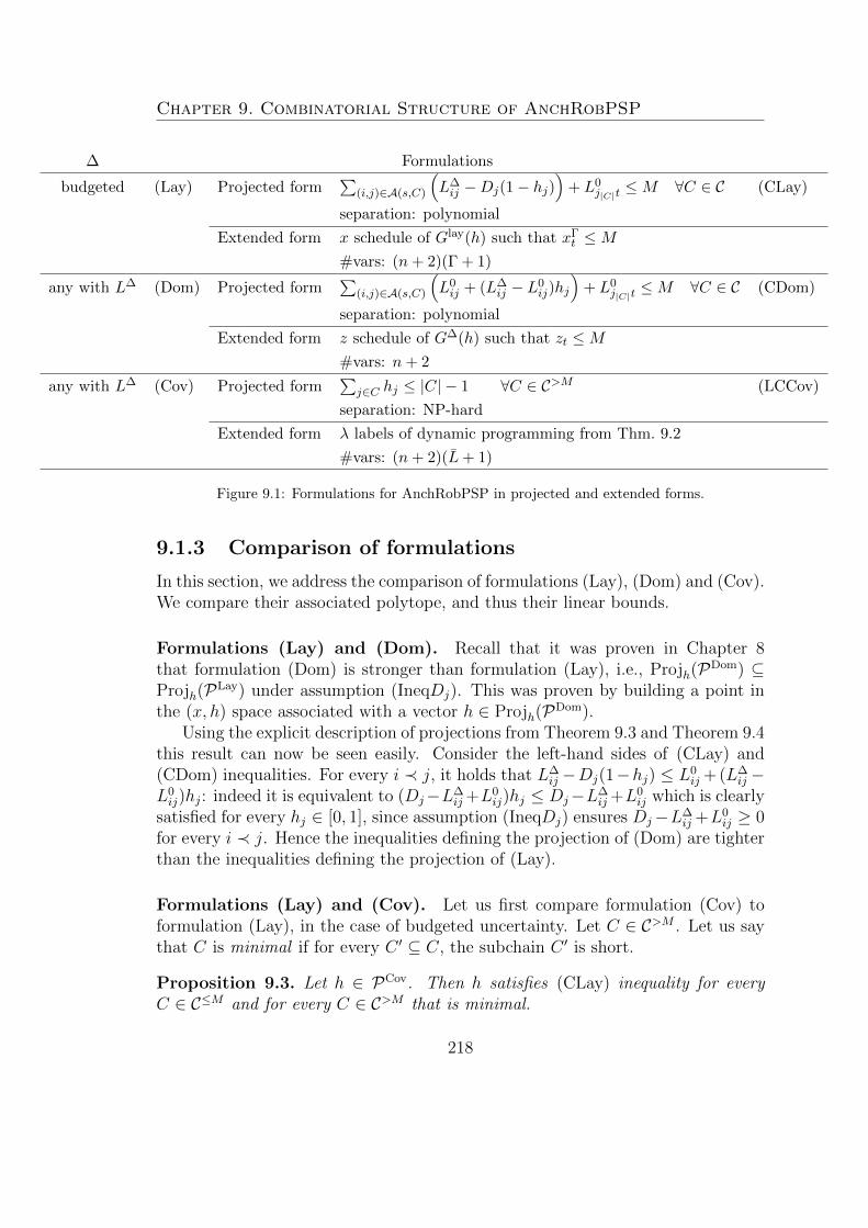
Chapter 9. Combinatorial Structure of AnchRobPSP
∆ Formulations
budgeted (Lay) Projected form∑
(i,j)∈A(s,C)
(L∆ij −Dj(1− hj)
)+ L0
j|C|t≤M ∀C ∈ C (CLay)
separation: polynomial
Extended form x schedule of Glay(h) such that xΓt ≤M
#vars: (n+ 2)(Γ + 1)
any with L∆ (Dom) Projected form∑
(i,j)∈A(s,C)
(L0ij + (L∆
ij − L0ij)hj
)+ L0
j|C|t≤M ∀C ∈ C (CDom)
separation: polynomial
Extended form z schedule of G∆(h) such that zt ≤M#vars: n+ 2
any with L∆ (Cov) Projected form∑
j∈C hj ≤ |C| − 1 ∀C ∈ C>M (LCCov)
separation: NP-hard
Extended form λ labels of dynamic programming from Thm. 9.2
#vars: (n+ 2)(L+ 1)
Figure 9.1: Formulations for AnchRobPSP in projected and extended forms.
9.1.3 Comparison of formulations
In this section, we address the comparison of formulations (Lay), (Dom) and (Cov).We compare their associated polytope, and thus their linear bounds.
Formulations (Lay) and (Dom). Recall that it was proven in Chapter 8that formulation (Dom) is stronger than formulation (Lay), i.e., Projh(PDom) ⊆Projh(PLay) under assumption (IneqDj). This was proven by building a point inthe (x, h) space associated with a vector h ∈ Projh(PDom).
Using the explicit description of projections from Theorem 9.3 and Theorem 9.4this result can now be seen easily. Consider the left-hand sides of (CLay) and(CDom) inequalities. For every i ≺ j, it holds that L∆
ij −Dj(1−hj) ≤ L0ij + (L∆
ij −L0ij)hj: indeed it is equivalent to (Dj−L∆
ij +L0ij)hj ≤ Dj−L∆
ij +L0ij which is clearly
satisfied for every hj ∈ [0, 1], since assumption (IneqDj) ensures Dj−L∆ij +L0
ij ≥ 0for every i ≺ j. Hence the inequalities defining the projection of (Dom) are tighterthan the inequalities defining the projection of (Lay).
Formulations (Lay) and (Cov). Let us first compare formulation (Cov) toformulation (Lay), in the case of budgeted uncertainty. Let C ∈ C>M . Let us saythat C is minimal if for every C ′ ⊆ C, the subchain C ′ is short.
Proposition 9.3. Let h ∈ PCov. Then h satisfies (CLay) inequality for everyC ∈ C≤M and for every C ∈ C>M that is minimal.
218
Chapter 9. Combinatorial Structure of AnchRobPSP
Proof. Let h ∈ PCov. Note that inequality (CLay) rewrites as∑j∈C Dj(1− hj) ≥ `∆(C)−M
The left-hand side is non-negative since h ∈ [0, 1]J . For C ∈ C≤M the right-handside `∆(C)−M is non-positive, so the inequality is satisfied by h.
Consider C ∈ C>M that is minimal. Let us prove the following claim: for everyj ∈ C, `∆(C) −M ≤ Dj. Fix some j ∈ C. Let us partition the chain C intoC≺j = {i ∈ C : i ≺ j}, {j} and C�j = {i ∈ C : j ≺ i}. Arcs from chain C areeither in C≺j ∪ {j} or C�j ∪ {j}. It holds that
`∆(C)−M = (`∆(C≺j ∪ {j})− L0jt) + (`∆(C�j ∪ {j})− L∆
sj)−M.
Note that the value LG(p+δ)(s, j) is greater than the length of any s−j path in G∆,
namely LG(p+δ)(s, j) ≥ `∆(C≺j ∪ {j}) − L0jt. Since Dj = LG(p+δ)(s, j) − L0
sj, we
have Dj ≥ `∆(C≺j ∪ {j})− L0jt − L0
sj. Hence
`∆(C)−M ≤ Dj + L0sj + `∆(C�j ∪ {j})− L∆
sj −M .
Denote by k the first vertex of C�j. It holds that L0sj + L∆
jk ≤ L∆sk by definition of
the L∆ values. Thus L0sj + `∆(C�j ∪ {j})−L∆
sj ≤ `∆(C�j). The subchain C�j is asubchain of C hence by assumption on C, it is short, i.e., `∆(C�j) ≤ M . Finallywe obtain `∆(C)−M ≤ Dj and the claim is proven.
Let us now prove the main result. It holds that∑
j∈C Dj(1−hj) ≥ Dj∗(∑
j∈C(1−hj)) where Dj∗ = minj∈C Dj. Since h ∈ PCov and C ∈ C>M , the (LCCov) in-equality gives
∑j∈C(1 − hj) ≥ 1. Then
∑j∈C Dj(1 − hj) ≥ Dj∗ ≥ `∆(C) −M
by the claim. This proves that h satisfies the (CLay) inequality associated withchain C.
An open question is whether h ∈ PCov also satisfies (CLay) for long chains thatare not minimal. If so, formulation (Cov) would be proven stronger than (Lay).Note that for a large enough value of the Dj values, formulation (Cov) would bestronger than (Lay).
Formulations (Dom) and (Cov). Let us now answer the question of the com-parison between the formulations (Cov) and (Dom).
Theorem 9.5. There exists an instance of AnchRobPSP where PCov and Projh(PDom)are not comparable, in the sense that
PCov \ Projh(PDom) 6= ∅ and Projh(PDom) \ PCov 6= ∅.
219
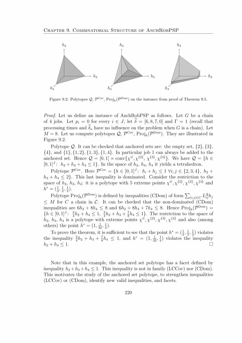
Chapter 9. Combinatorial Structure of AnchRobPSP
h2
h3
h4
h2
h3
h4
h2
h3
h4
Figure 9.2: Polytopes Q, PCov, Projh(PDom) on the instance from proof of Theorem 9.5.
Proof. Let us define an instance of AnchRobPSP as follows. Let G be a chainof 4 jobs. Let pi = 0 for every i ∈ J , let δ = [6, 8, 7, 0] and Γ = 1 (recall that
processing times and δn have no influence on the problem when G is a chain). LetM = 8. Let us compute polytopes Q, PCov, Projh(PDom). They are illustrated inFigure 9.2.
Polytope Q. It can be checked that anchored sets are: the empty set, {2}, {3},{4}, and {1}, {1, 2}, {1, 3}, {1, 4}. In particular job 1 can always be added to theanchored set. Hence Q = [0, 1] × conv{χ∅, χ{2}, χ{3}, χ{4}}. We have Q = {h ∈[0, 1]J : h2 + h3 + h4 ≤ 1}. In the space of h2, h3, h4 it yields a tetrahedron.
Polytope PCov. Here PCov = {h ∈ [0, 1]J : hi + hj ≤ 1 ∀i, j ∈ {2, 3, 4}, h2 +h3 + h4 ≤ 2}. This last inequality is dominated. Consider the restriction to thespace of h2, h3, h4: it is a polytope with 5 extreme points χ∅, χ{2}, χ{3}, χ{4} andh∗ = (1
2, 1
2, 1
2).
Polytope Projh(PDom) is defined by inequalities (CDom) of form∑
(i,j)∈C L∆ijhj
≤ M for C a chain in C. It can be checked that the non-dominated (CDom)inequalities are 6h2 + 8h4 ≤ 8 and 6h2 + 8h3 + 7h4 ≤ 8. Hence Projh(PDom) ={h ∈ [0, 1]J : 3
4h2 + h4 ≤ 1, 3
4h2 + h3 + 7
8h4 ≤ 1}. The restriction to the space of
h2, h3, h4 is a polytope with extreme points χ∅, χ{2}, χ{3}, χ{4} and also (amongothers) the point h◦ = (1, 1
32, 1
4).
To prove the theorem, it is sufficient to see that the point h∗ = (12, 1
2, 1
2) violates
the inequality 34h2 + h3 + 7
8h4 ≤ 1, and h◦ = (1, 1
32, 1
4) violates the inequality
h2 + h4 ≤ 1.
Note that in this example, the anchored set polytope has a facet defined byinequality h2 +h3 +h4 ≤ 1. This inequality is not in family (LCCov) nor (CDom).This motivates the study of the anchored set polytope, to strengthen inequalities(LCCov) or (CDom), identify new valid inequalities, and facets.
220
Chapter 9. Combinatorial Structure of AnchRobPSP
9.2 Polyhedral study of the polytope of
anchored sets
In this section we study the polytope
Q = conv{χH : H anchored set}.In Section 9.2.1 simple facets are identified. In Section 9.2.2 polyhedral char-acterization cases are considered and a minimal description of Q is given. InSection 9.2.3 and Section 9.2.4 we propose new valid inequalities to strengthen(LCCov) inequalities.
9.2.1 Preliminaries
Let us start with some standard polyhedral results on Q. Let Jout = {i ∈ J : L∆si+
L0it > M}. Job i is in Jout when the singleton {i} is not an anchored set. Note
that if i ∈ Jout then no anchored set contains job i. Then the dimension of Q is|J | − |Jout|. Indeed the polytope Q is included in
⋂i∈Jout{hi = 0} hence it has
dimension at most n − |Jout|. The vectors χ{i} for i /∈ Jout are in Q and linearlyindependent.
Proposition 9.4. The inequality hi ≥ 0 defines a facet of Q for every i ∈ J .
Proof. The vectors χ∅, χ{j} for j 6= i are n vectors of the face Q ∩ {h : hi = 0}that are affinely independent.
Proposition 9.5. Every facet of Q distinct from non-negativity can be written asαTh ≤ β with α ∈ RJ
+ and β ∈ R+.
Proof. Consider the facet F = Q ∩ {αTh = β} with any α, β. If all points inF satisfy hi = 0 for some i ∈ J then the facet is induced by the non-negativityconstraint hi ≥ 0. Otherwise, for i ∈ J there exists h ∈ F such that hi = 1, andαi + αT (h− χ{i}) = β. Since h− χ{i} ∈ Q, αT (h− χ{i}) ≤ β, hence αi ≥ 0. Thenβ ≥ 0 follows.
Proposition 9.6. Let i ∈ J . The inequality hi ≤ 1 defines a facet if and only iffor every j 6= i, the pair {i, j} can be anchored.
Proof. If {i, j} is not anchored for some j 6= i, then the inequality hi + hj ≤ 1is valid for Q and it dominates hi ≤ 1. Assume {i, j} can be anchored for everyj 6= i. Consider the family of n vectors χ{i}, χ{i,j} for j 6= i: they are affinelyindependent vectors of Q satisfying hi = 1. Hence hi ≤ 1 defines a facet.
Remark that the inequality hi + hj ≤ 1 used in the necessity proof is of form(LCCov); indeed it writes h(C) ≤ |C| − 1 with C = (s, i, j, t) (w.l.o.g. i ≺ j). Itholds that C ∈ C>M when {i, j} is not anchored.
221
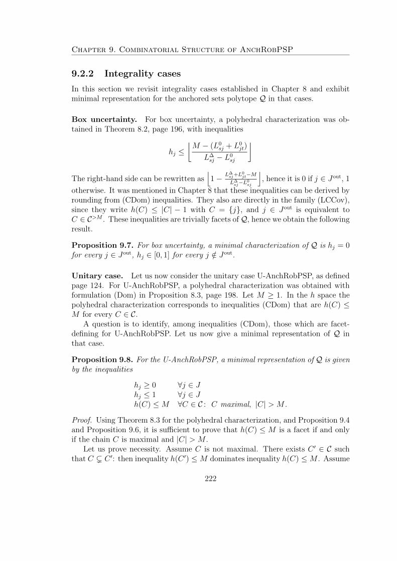
Chapter 9. Combinatorial Structure of AnchRobPSP
9.2.2 Integrality cases
In this section we revisit integrality cases established in Chapter 8 and exhibitminimal representation for the anchored sets polytope Q in that cases.
Box uncertainty. For box uncertainty, a polyhedral characterization was ob-tained in Theorem 8.2, page 196, with inequalities
hj ≤⌊M − (L0
sj + L0jt)
L∆sj − L0
sj
⌋
The right-hand side can be rewritten as⌊1− L∆
sj+L0jt−M
L∆sj−L0
sj
⌋, hence it is 0 if j ∈ Jout, 1
otherwise. It was mentioned in Chapter 8 that these inequalities can be derived byrounding from (CDom) inequalities. They also are directly in the family (LCCov),since they write h(C) ≤ |C| − 1 with C = {j}, and j ∈ Jout is equivalent toC ∈ C>M . These inequalities are trivially facets ofQ, hence we obtain the followingresult.
Proposition 9.7. For box uncertainty, a minimal characterization of Q is hj = 0for every j ∈ Jout, hj ∈ [0, 1] for every j /∈ Jout.
Unitary case. Let us now consider the unitary case U-AnchRobPSP, as definedpage 124. For U-AnchRobPSP, a polyhedral characterization was obtained withformulation (Dom) in Proposition 8.3, page 198. Let M ≥ 1. In the h space thepolyhedral characterization corresponds to inequalities (CDom) that are h(C) ≤M for every C ∈ C.
A question is to identify, among inequalities (CDom), those which are facet-defining for U-AnchRobPSP. Let us now give a minimal representation of Q inthat case.
Proposition 9.8. For the U-AnchRobPSP, a minimal representation of Q is givenby the inequalities
hj ≥ 0 ∀j ∈ Jhj ≤ 1 ∀j ∈ Jh(C) ≤M ∀C ∈ C : C maximal, |C| > M .
Proof. Using Theorem 8.3 for the polyhedral characterization, and Proposition 9.4and Proposition 9.6, it is sufficient to prove that h(C) ≤ M is a facet if and onlyif the chain C is maximal and |C| > M .
Let us prove necessity. Assume C is not maximal. There exists C ′ ∈ C suchthat C ( C ′: then inequality h(C ′) ≤M dominates inequality h(C) ≤M . Assume
222
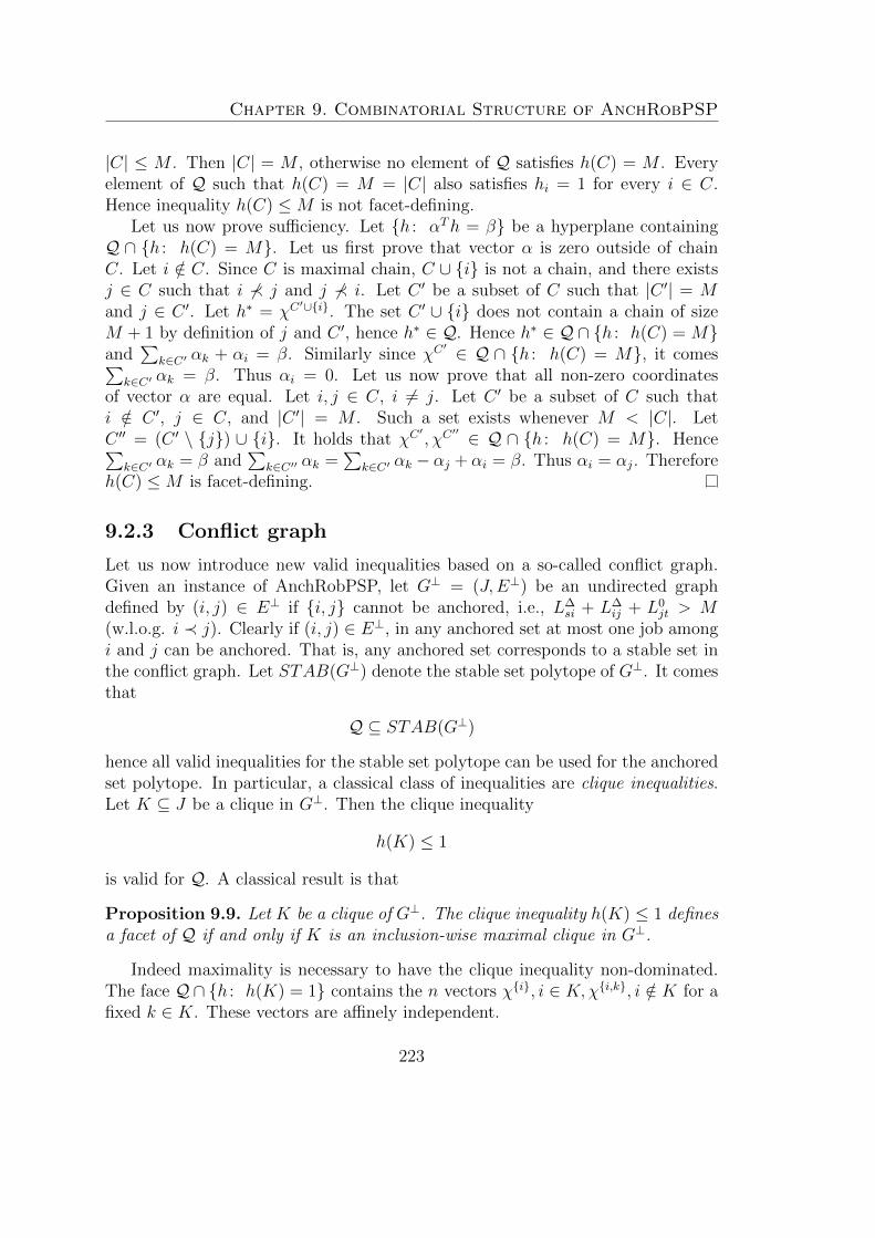
Chapter 9. Combinatorial Structure of AnchRobPSP
|C| ≤ M . Then |C| = M , otherwise no element of Q satisfies h(C) = M . Everyelement of Q such that h(C) = M = |C| also satisfies hi = 1 for every i ∈ C.Hence inequality h(C) ≤M is not facet-defining.
Let us now prove sufficiency. Let {h : αTh = β} be a hyperplane containingQ ∩ {h : h(C) = M}. Let us first prove that vector α is zero outside of chainC. Let i /∈ C. Since C is maximal chain, C ∪ {i} is not a chain, and there existsj ∈ C such that i 6≺ j and j 6≺ i. Let C ′ be a subset of C such that |C ′| = Mand j ∈ C ′. Let h∗ = χC
′∪{i}. The set C ′ ∪ {i} does not contain a chain of sizeM + 1 by definition of j and C ′, hence h∗ ∈ Q. Hence h∗ ∈ Q ∩ {h : h(C) = M}and
∑k∈C′ αk + αi = β. Similarly since χC
′ ∈ Q ∩ {h : h(C) = M}, it comes∑k∈C′ αk = β. Thus αi = 0. Let us now prove that all non-zero coordinates
of vector α are equal. Let i, j ∈ C, i 6= j. Let C ′ be a subset of C such thati /∈ C ′, j ∈ C, and |C ′| = M . Such a set exists whenever M < |C|. LetC ′′ = (C ′ \ {j}) ∪ {i}. It holds that χC
′, χC
′′ ∈ Q ∩ {h : h(C) = M}. Hence∑k∈C′ αk = β and
∑k∈C′′ αk =
∑k∈C′ αk − αj + αi = β. Thus αi = αj. Therefore
h(C) ≤M is facet-defining.
9.2.3 Conflict graph
Let us now introduce new valid inequalities based on a so-called conflict graph.Given an instance of AnchRobPSP, let G⊥ = (J,E⊥) be an undirected graphdefined by (i, j) ∈ E⊥ if {i, j} cannot be anchored, i.e., L∆
si + L∆ij + L0
jt > M(w.l.o.g. i ≺ j). Clearly if (i, j) ∈ E⊥, in any anchored set at most one job amongi and j can be anchored. That is, any anchored set corresponds to a stable set inthe conflict graph. Let STAB(G⊥) denote the stable set polytope of G⊥. It comesthat
Q ⊆ STAB(G⊥)
hence all valid inequalities for the stable set polytope can be used for the anchoredset polytope. In particular, a classical class of inequalities are clique inequalities.Let K ⊆ J be a clique in G⊥. Then the clique inequality
h(K) ≤ 1
is valid for Q. A classical result is that
Proposition 9.9. Let K be a clique of G⊥. The clique inequality h(K) ≤ 1 definesa facet of Q if and only if K is an inclusion-wise maximal clique in G⊥.
Indeed maximality is necessary to have the clique inequality non-dominated.The face Q∩ {h : h(K) = 1} contains the n vectors χ{i}, i ∈ K,χ{i,k}, i /∈ K for afixed k ∈ K. These vectors are affinely independent.
223
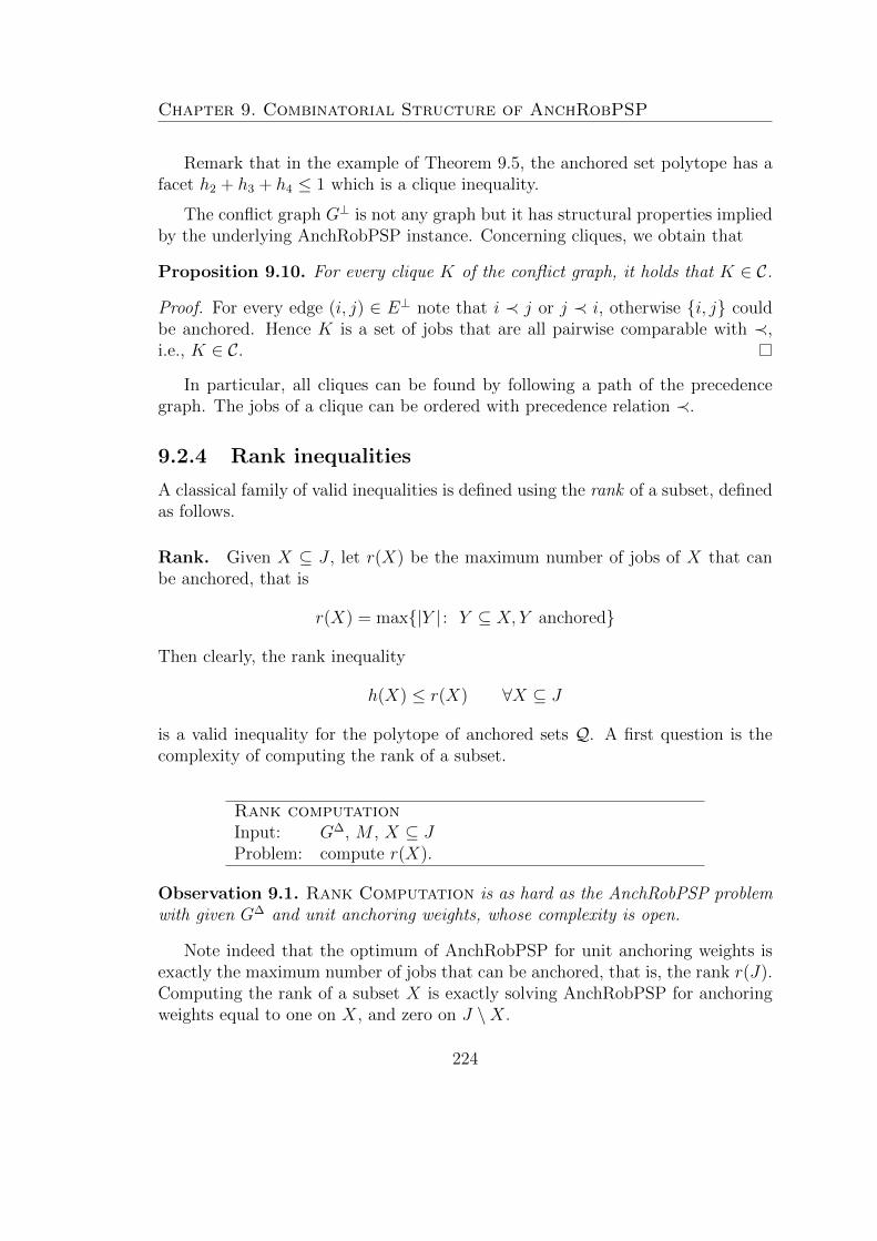
Chapter 9. Combinatorial Structure of AnchRobPSP
Remark that in the example of Theorem 9.5, the anchored set polytope has afacet h2 + h3 + h4 ≤ 1 which is a clique inequality.
The conflict graph G⊥ is not any graph but it has structural properties impliedby the underlying AnchRobPSP instance. Concerning cliques, we obtain that
Proposition 9.10. For every clique K of the conflict graph, it holds that K ∈ C.
Proof. For every edge (i, j) ∈ E⊥ note that i ≺ j or j ≺ i, otherwise {i, j} couldbe anchored. Hence K is a set of jobs that are all pairwise comparable with ≺,i.e., K ∈ C.
In particular, all cliques can be found by following a path of the precedencegraph. The jobs of a clique can be ordered with precedence relation ≺.
9.2.4 Rank inequalities
A classical family of valid inequalities is defined using the rank of a subset, definedas follows.
Rank. Given X ⊆ J , let r(X) be the maximum number of jobs of X that canbe anchored, that is
r(X) = max{|Y | : Y ⊆ X, Y anchored}
Then clearly, the rank inequality
h(X) ≤ r(X) ∀X ⊆ J
is a valid inequality for the polytope of anchored sets Q. A first question is thecomplexity of computing the rank of a subset.
Rank computationInput: G∆, M , X ⊆ JProblem: compute r(X).
Observation 9.1. Rank Computation is as hard as the AnchRobPSP problemwith given G∆ and unit anchoring weights, whose complexity is open.
Note indeed that the optimum of AnchRobPSP for unit anchoring weights isexactly the maximum number of jobs that can be anchored, that is, the rank r(J).Computing the rank of a subset X is exactly solving AnchRobPSP for anchoringweights equal to one on X, and zero on J \X.
224
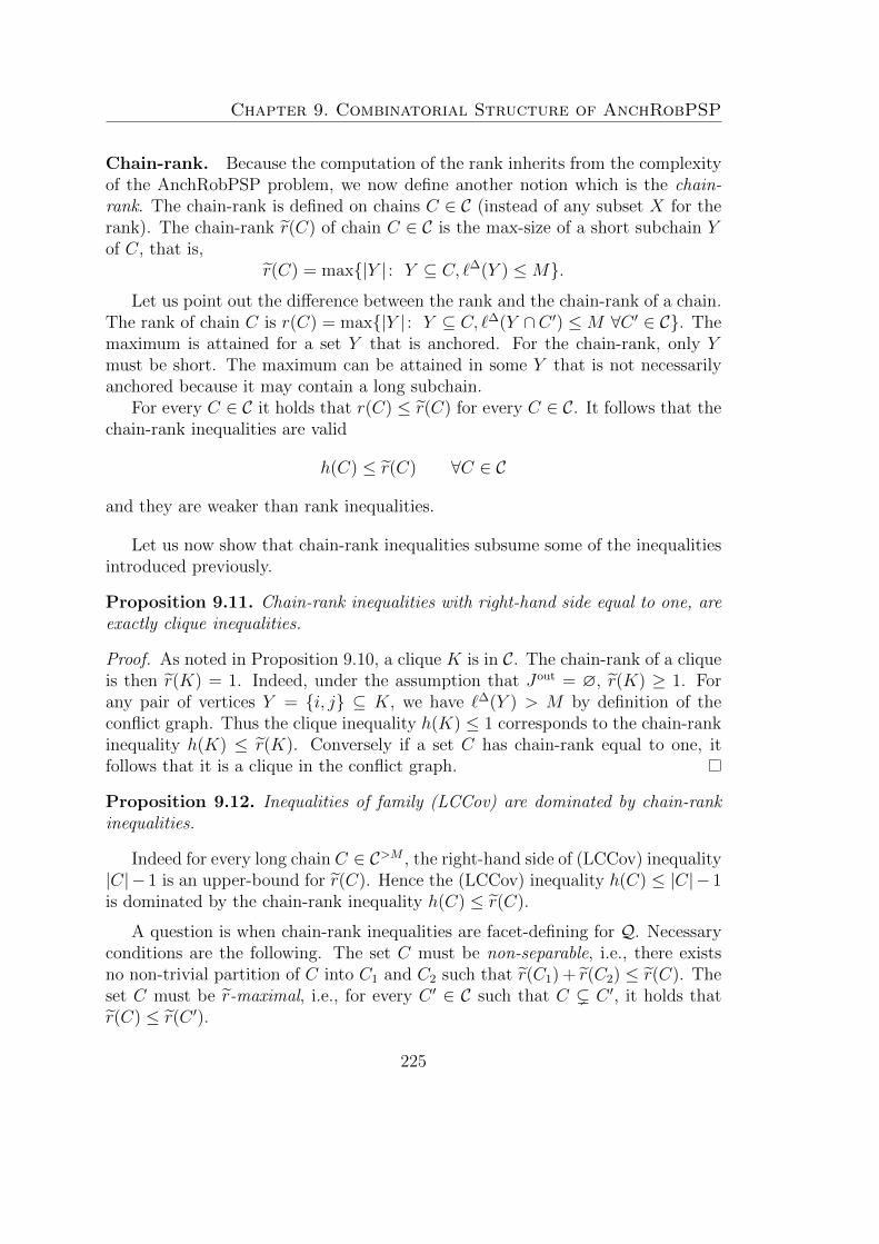
Chapter 9. Combinatorial Structure of AnchRobPSP
Chain-rank. Because the computation of the rank inherits from the complexityof the AnchRobPSP problem, we now define another notion which is the chain-rank. The chain-rank is defined on chains C ∈ C (instead of any subset X for therank). The chain-rank r(C) of chain C ∈ C is the max-size of a short subchain Yof C, that is,
r(C) = max{|Y | : Y ⊆ C, `∆(Y ) ≤M}.
Let us point out the difference between the rank and the chain-rank of a chain.The rank of chain C is r(C) = max{|Y | : Y ⊆ C, `∆(Y ∩C ′) ≤M ∀C ′ ∈ C}. Themaximum is attained for a set Y that is anchored. For the chain-rank, only Ymust be short. The maximum can be attained in some Y that is not necessarilyanchored because it may contain a long subchain.
For every C ∈ C it holds that r(C) ≤ r(C) for every C ∈ C. It follows that thechain-rank inequalities are valid
h(C) ≤ r(C) ∀C ∈ C
and they are weaker than rank inequalities.
Let us now show that chain-rank inequalities subsume some of the inequalitiesintroduced previously.
Proposition 9.11. Chain-rank inequalities with right-hand side equal to one, areexactly clique inequalities.
Proof. As noted in Proposition 9.10, a clique K is in C. The chain-rank of a cliqueis then r(K) = 1. Indeed, under the assumption that Jout = ∅, r(K) ≥ 1. Forany pair of vertices Y = {i, j} ⊆ K, we have `∆(Y ) > M by definition of theconflict graph. Thus the clique inequality h(K) ≤ 1 corresponds to the chain-rankinequality h(K) ≤ r(K). Conversely if a set C has chain-rank equal to one, itfollows that it is a clique in the conflict graph.
Proposition 9.12. Inequalities of family (LCCov) are dominated by chain-rankinequalities.
Indeed for every long chain C ∈ C>M , the right-hand side of (LCCov) inequality|C|− 1 is an upper-bound for r(C). Hence the (LCCov) inequality h(C) ≤ |C|− 1is dominated by the chain-rank inequality h(C) ≤ r(C).
A question is when chain-rank inequalities are facet-defining for Q. Necessaryconditions are the following. The set C must be non-separable, i.e., there existsno non-trivial partition of C into C1 and C2 such that r(C1) + r(C2) ≤ r(C). Theset C must be r-maximal, i.e., for every C ′ ∈ C such that C ( C ′, it holds thatr(C) ≤ r(C ′).
225
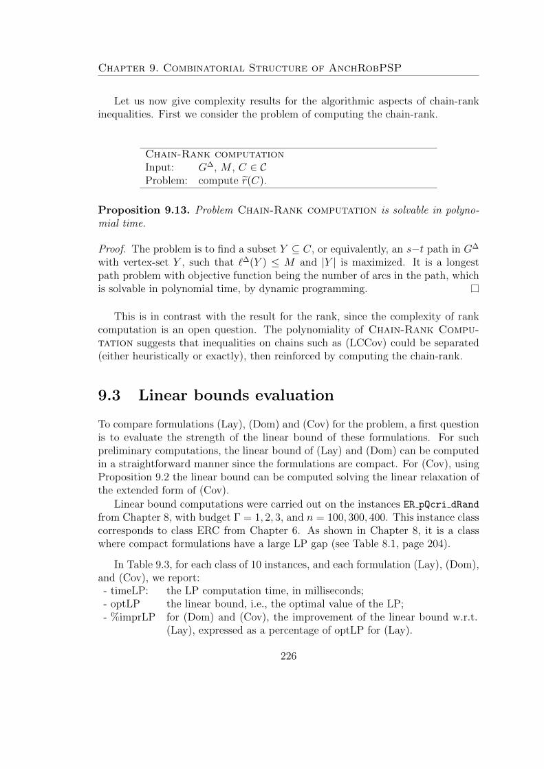
Chapter 9. Combinatorial Structure of AnchRobPSP
Let us now give complexity results for the algorithmic aspects of chain-rankinequalities. First we consider the problem of computing the chain-rank.
Chain-Rank computationInput: G∆, M , C ∈ CProblem: compute r(C).
Proposition 9.13. Problem Chain-Rank computation is solvable in polyno-mial time.
Proof. The problem is to find a subset Y ⊆ C, or equivalently, an s−t path in G∆
with vertex-set Y , such that `∆(Y ) ≤ M and |Y | is maximized. It is a longestpath problem with objective function being the number of arcs in the path, whichis solvable in polynomial time, by dynamic programming.
This is in contrast with the result for the rank, since the complexity of rankcomputation is an open question. The polynomiality of Chain-Rank Compu-tation suggests that inequalities on chains such as (LCCov) could be separated(either heuristically or exactly), then reinforced by computing the chain-rank.
9.3 Linear bounds evaluation
To compare formulations (Lay), (Dom) and (Cov) for the problem, a first questionis to evaluate the strength of the linear bound of these formulations. For suchpreliminary computations, the linear bound of (Lay) and (Dom) can be computedin a straightforward manner since the formulations are compact. For (Cov), usingProposition 9.2 the linear bound can be computed solving the linear relaxation ofthe extended form of (Cov).
Linear bound computations were carried out on the instances ER pQcri dRand
from Chapter 8, with budget Γ = 1, 2, 3, and n = 100, 300, 400. This instance classcorresponds to class ERC from Chapter 6. As shown in Chapter 8, it is a classwhere compact formulations have a large LP gap (see Table 8.1, page 204).
In Table 9.3, for each class of 10 instances, and each formulation (Lay), (Dom),and (Cov), we report:- timeLP: the LP computation time, in milliseconds;- optLP the linear bound, i.e., the optimal value of the LP;- %imprLP for (Dom) and (Cov), the improvement of the linear bound w.r.t.
(Lay), expressed as a percentage of optLP for (Lay).
226
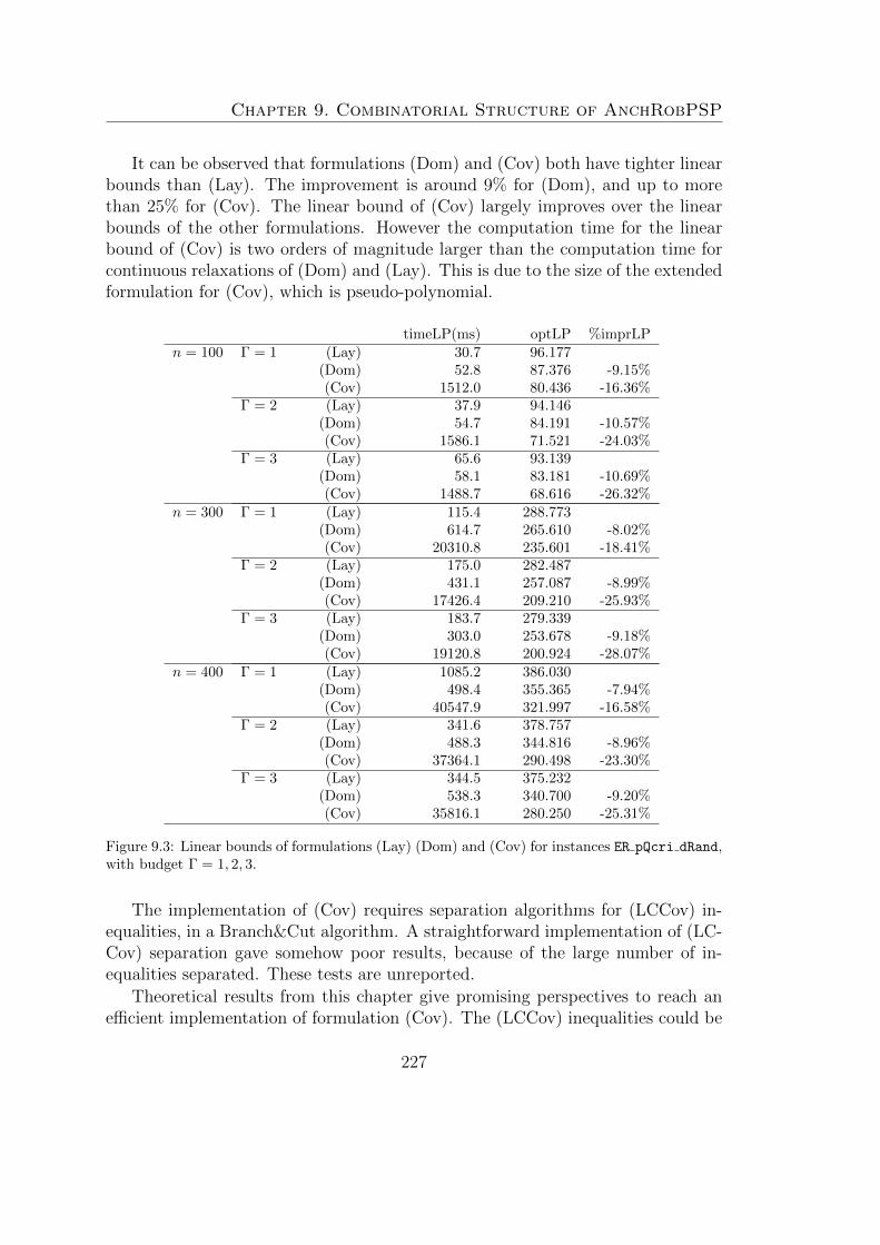
Chapter 9. Combinatorial Structure of AnchRobPSP
It can be observed that formulations (Dom) and (Cov) both have tighter linearbounds than (Lay). The improvement is around 9% for (Dom), and up to morethan 25% for (Cov). The linear bound of (Cov) largely improves over the linearbounds of the other formulations. However the computation time for the linearbound of (Cov) is two orders of magnitude larger than the computation time forcontinuous relaxations of (Dom) and (Lay). This is due to the size of the extendedformulation for (Cov), which is pseudo-polynomial.
timeLP(ms) optLP %imprLPn = 100 Γ = 1 (Lay) 30.7 96.177
(Dom) 52.8 87.376 -9.15%(Cov) 1512.0 80.436 -16.36%
Γ = 2 (Lay) 37.9 94.146(Dom) 54.7 84.191 -10.57%(Cov) 1586.1 71.521 -24.03%
Γ = 3 (Lay) 65.6 93.139(Dom) 58.1 83.181 -10.69%(Cov) 1488.7 68.616 -26.32%
n = 300 Γ = 1 (Lay) 115.4 288.773(Dom) 614.7 265.610 -8.02%(Cov) 20310.8 235.601 -18.41%
Γ = 2 (Lay) 175.0 282.487(Dom) 431.1 257.087 -8.99%(Cov) 17426.4 209.210 -25.93%
Γ = 3 (Lay) 183.7 279.339(Dom) 303.0 253.678 -9.18%(Cov) 19120.8 200.924 -28.07%
n = 400 Γ = 1 (Lay) 1085.2 386.030(Dom) 498.4 355.365 -7.94%(Cov) 40547.9 321.997 -16.58%
Γ = 2 (Lay) 341.6 378.757(Dom) 488.3 344.816 -8.96%(Cov) 37364.1 290.498 -23.30%
Γ = 3 (Lay) 344.5 375.232(Dom) 538.3 340.700 -9.20%(Cov) 35816.1 280.250 -25.31%
Figure 9.3: Linear bounds of formulations (Lay) (Dom) and (Cov) for instances ER pQcri dRand,with budget Γ = 1, 2, 3.
The implementation of (Cov) requires separation algorithms for (LCCov) in-equalities, in a Branch&Cut algorithm. A straightforward implementation of (LC-Cov) separation gave somehow poor results, because of the large number of in-equalities separated. These tests are unreported.
Theoretical results from this chapter give promising perspectives to reach anefficient implementation of formulation (Cov). The (LCCov) inequalities could be
227
Chapter 9. Combinatorial Structure of AnchRobPSP
reinforced using polyhedral results, e.g., chain-rank inequalities. We note that theevaluation of formulations would require a specific work on the instance bench-mark. Indeed numerical performance of formulations are likely to depend stronglyon the precedence graph, its density, or the numerical values of deviations. An-other perspective is to combine formulations (Dom) and (Cov). Indeed as notedin Theorem 9.5 the two formulations are not comparable. A hybrid formulationcould benefit from (Dom) to ensure validity with a compact number of variablesand constraints, and from the tight linear bound of (Cov).
Conclusion
We studied the AnchRobPSP problem in the space of anchoring variables. Thesevariables are the combinatorial decisions in AnchRobPSP. First a new cover expo-nential formulation was proposed. For formulations obtained previously, we wereable to establish explicit projections onto the space of anchoring variables. This al-lows for a comparison of the formulations’ polytopes, in a common variable space.We highlighted the connection between longest path separation problems, andadditional variables appearing in extended formulations. The variety of valid in-equalities obtained for the problem motivated a polyhedral study of the anchoredset polytope. In special cases with a polyhedral characterization, the list of allfacets was obtained. New inequalities were proposed based on conflict graph orrank, their facial properties were considered.
Theoretical questions could be further investigated on the anchored set poly-tope. Concepts such as the conflict graph or the rank are quite generic; a questionis thus to analyze their structure in the case of AnchRobPSP to obtain more dedi-cated results. Another perspective is to investigate the similarity with the knapsackproblem, since anchoring variables must satisfy knapsack constraints along chains,as shown, e.g., by (CDom) inequalities.
A research direction is also to perform numerical experiments to assess the per-formance of exponential formulations. An efficient implementation of separationalgorithms for (Cov) could lead to an efficient Branch&Cut algorithm, benefitingfrom the tight linear bound of this formulation. Since (Dom) and (Cov) are notcomparable, we could design a hybrid formulation, where a compact formulationsuch as (Dom) is used for validity, and separation of (Cov) is used for reinforce-ment.
228


Chapter 9. Combinatorial Structure of AnchRobPSP
230
Conclusion and research perspectives
In this thesis we investigated anchored solutions for discrete optimization problemsunder uncertainty. Anchored solutions appear to be a quite simple yet practicallyattractive concept, and a new idea in robust optimization. The anchor-robust prob-lem produces a baseline solution with bounded cost, and a subset of anchored de-cisions. As emphasized throughout the manuscript, it is a middle ground betweenstatic and adjustable-robustness, and it gives control over the price of robustness.The anchor-robust problem belongs to the class of robust 2-stage problems, whichis computationally challenging. In spite of its conceptual simplicity, the problemcan be very hard to solve. We thus thoroughly investigated the tractability ofthe anchor-robust problem, first by a study of its complexity and combinatorialstructure, then by the design of algorithmic approaches based on mixed-integerprogramming. This led to a dedicated work, first on combinatorial problems suchas spanning trees and matchings, then on project scheduling problems.
For problems written as integer programs in binary variables, we studied thecomplexity of anchor-reoptimization and anchor-robust optimization under costuncertainty. We investigated formulations through linear programs (via polyhedralcharacterization) or mixed-integer programs (via reformulations). The focus wason polynomial combinatorial problems, such as matroid bases.
An important research direction is to extend the results to other combinatorialproblems, and in particular NP-hard ones. For the anchor-reoptimization problem,a question is to study the polytope of k-red classical problems, for which new facetsarise, starting with the k-red matching polytope. For the anchor-robust problem,a question is to extend the applicability range of the anchor-robust problem to anycombinatorial problem with a valid formulation. This implies to design algorithmicapproaches where an efficient polyhedral characterization of the original problemis not explicitly required. The price of anchor-robustness should also be furtherinvestigated, both theoretically and based on numerical experiments.
For project scheduling problems with starting times as continuous variables, theanchoring level led to new rescheduling problems. We extended the polynomialityresult to generalized precedence and tolerance. We pointed out the boundary
231
Conclusion and perspectives
between polynomial and NP-hard anchored rescheduling problems. The anchor-robust approach was then investigated for project scheduling. It differentiates itselffrom the project scheduling literature, that contained mainly proactive problemswith continuous stability measures, or adjustable-robust approaches producing nobaseline. An important part of the thesis is dedicated to anchor-robust projectscheduling.
We first proposed the Anchor-Robust Project Scheduling Problem (AnchRob-PSP) in the case of precedence constraints. This problem can be seen as thecore of anchor-robustness for project scheduling. We studied the combinatorialstructure of the problem and proposed two dedicated graph models, one basedon the transitive closure of the precedence graph, the other one on a layeredgraph dedicated to budgeted uncertainty. The complexity of AnchRobPSP wasanalyzed for various polyhedral uncertainty sets (box, budgeted, any polytope).In particular, we highlighted the connection with the complexity of computing theworst-case value of longest paths in the precedence graph. Polynomial cases wereexhibited, depending on the uncertainty set and the precedence graph.
We proposed mixed-integer programming formulations for AnchRobPSP, stren-gthened by a study of their polyhedral properties. We obtained first a formulationbased on the layered graph, valid for budgeted uncertainty. We then providedother formulations that are applicable to more uncertainty sets, based on thetransitive closure graph model. A dominance property was a keypoint to obtaina stronger formulation, which is still compact. A non-compact formulation wasalso proposed. We showed the connection between the different variable spaces,through projections or extensions of our formulations. This leads to a variety ofMIP tools for the problem. They appear to be quite efficient in practice, whichis a good sign for the practical implementability of anchor-robustness in projectscheduling.
For the AnchRobPSP, we observed the very good numerical performance ofcompact MIP formulations. An open question is whether the AnchRobPSP isstrongly NP-hard. In particular, the complexity of the AnchRobPSP under bud-geted uncertainty and unit anchoring weights, is open. A related perspective is tofurther investigate the anchored set polytope.
We extended the anchor-robust approach to the Resource-Constraint ProjectScheduling Problem, which is strongly NP-hard. In the design of an anchor-robustproblem, the keypoint was to consider restricted reoptimization, and namely, re-optimization with fixed resource flow. This simplifies the recourse problem, asshown by the complexity analysis of anchored rescheduling problems. Most resultsobtained on the AnchRobPSP problem then carried over to the Anchor-RobustRCPSP, such as the layered graph for budgeted uncertainty. We proposed exactand heuristic approaches, for both the Adjustable-Robust RCPSP and the Anchor-
232
Conclusion and perspectives
Robust RCPSP. Numerical experiments showed that for exact approaches, thecomputational cost for solving the Adjustable-Robust RCPSP or Anchor-RobustRCPSP was not a lot larger than the original RCPSP. The good quality of heuris-tic solutions was also highlighted. This is a robustness toolbox that can be usedin any practical application of the RCPSP. We highlighted the relevance of theAnchor-Robust RCPSP on an industrial use case at EDF.
A research perspective is to further improve the proposed algorithms on hardinstances of the Anchor-Robust RCPSP. A combination of the proposed tools canbe designed, benefiting from the efficiency of rule-based heuristics for the RCPSP,and mixed-integer programming for anchor-robustness.
A broader perspective is to extend the anchor-robust approach to other schedul-ing problems. Note that a specific attention should then be given to the definitionof anchored decisions, in the design of new anchor-robust problems. For instancethe definition we chose for the RCPSP is structurally based on the resource flowand processing time uncertainty. We may want, e.g., to consider a tolerance inthe definition of anchored jobs, as done in rescheduling. Resources can also betreated differently, with non-renewable resources, or resource leveling problemswhere the objective is to minimize the maximum consumption of resources. Un-certainty on resources (e.g., machine breakdowns) is another research direction ofpractical interest. Finally anchor-robustness could have an applicative interest onother problems such as production planning problems, combining combinatorialdecisions and scheduling decisions.
233

Conclusion and perspectives
234
Appendix
Extended computational results for the
Adjustable-Robust RCPSP
Let us present complete computational results for solving the Adjustable-RobustRCPSP with MIP formulation (Fadj). The computational settings are those de-scribed in Chapter 7, page 161. In Tables 9.1, 9.2, 9.3 are reported the results forΓ = 3, 5, 7 respectively. For each instance class j30x, x ∈ {1, . . . , 48}, we indicatefor (Fadj):
– the corresponding parameters NC, RF, RS;– solved: the number of instances solved to optimality (out of 10);– time: the computation time averaged on instances solved to optimality in
seconds;– unsolved = 10 - solved– gap: the final gap, averaged on instances not solved to optimality.
The results are presented in aggregated form in Chapter 7, e.g., in Table 7.1.
235
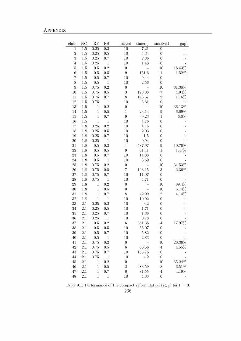
Appendix
class NC RF RS solved time(s) unsolved gap1 1.5 0.25 0.2 10 7.21 0 -2 1.5 0.25 0.5 10 4.34 0 -3 1.5 0.25 0.7 10 2.36 0 -4 1.5 0.25 1 10 1.43 0 -5 1.5 0.5 0.2 0 - 10 16.43%6 1.5 0.5 0.5 9 151.6 1 1.52%7 1.5 0.5 0.7 10 9.44 0 -8 1.5 0.5 1 10 2.56 0 -9 1.5 0.75 0.2 0 - 10 31.38%
10 1.5 0.75 0.5 3 198.88 7 4.94%11 1.5 0.75 0.7 8 146.67 2 1.76%12 1.5 0.75 1 10 5.31 0 -13 1.5 1 0.2 0 - 10 36.13%14 1.5 1 0.5 1 23.14 9 6.69%15 1.5 1 0.7 9 39.23 1 6.0%16 1.5 1 1 10 4.76 0 -17 1.8 0.25 0.2 10 4.15 0 -18 1.8 0.25 0.5 10 2.03 0 -19 1.8 0.25 0.7 10 1.5 0 -20 1.8 0.25 1 10 0.94 0 -21 1.8 0.5 0.2 1 587.97 9 10.76%22 1.8 0.5 0.5 9 61.41 1 1.47%23 1.8 0.5 0.7 10 14.33 0 -24 1.8 0.5 1 10 3.69 0 -25 1.8 0.75 0.2 0 - 10 31.53%26 1.8 0.75 0.5 7 193.15 3 2.36%27 1.8 0.75 0.7 10 11.97 0 -28 1.8 0.75 1 10 4.71 0 -29 1.8 1 0.2 0 - 10 39.4%30 1.8 1 0.5 0 - 10 5.74%31 1.8 1 0.7 8 42.99 2 4.14%32 1.8 1 1 10 10.92 0 -33 2.1 0.25 0.2 10 3.2 0 -34 2.1 0.25 0.5 10 1.71 0 -35 2.1 0.25 0.7 10 1.36 0 -36 2.1 0.25 1 10 0.78 0 -37 2.1 0.5 0.2 6 361.35 4 17.97%38 2.1 0.5 0.5 10 55.07 0 -39 2.1 0.5 0.7 10 5.82 0 -40 2.1 0.5 1 10 2.83 0 -41 2.1 0.75 0.2 0 - 10 26.36%42 2.1 0.75 0.5 6 66.56 4 4.55%43 2.1 0.75 0.7 10 155.76 0 -44 2.1 0.75 1 10 4.2 0 -45 2.1 1 0.2 0 - 10 35.24%46 2.1 1 0.5 2 483.59 8 6.51%47 2.1 1 0.7 6 81.55 4 4.19%48 2.1 1 1 10 4.33 0 -
Table 9.1: Performance of the compact reformulation (Fadj) for Γ = 3.
236
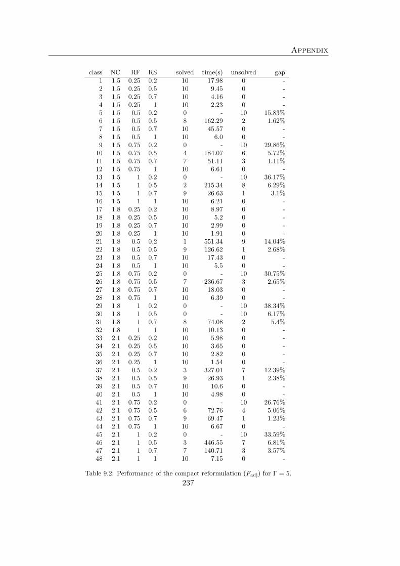
Appendix
class NC RF RS solved time(s) unsolved gap1 1.5 0.25 0.2 10 17.98 0 -2 1.5 0.25 0.5 10 9.45 0 -3 1.5 0.25 0.7 10 4.16 0 -4 1.5 0.25 1 10 2.23 0 -5 1.5 0.5 0.2 0 - 10 15.83%6 1.5 0.5 0.5 8 162.29 2 1.62%7 1.5 0.5 0.7 10 45.57 0 -8 1.5 0.5 1 10 6.0 0 -9 1.5 0.75 0.2 0 - 10 29.86%
10 1.5 0.75 0.5 4 184.07 6 5.72%11 1.5 0.75 0.7 7 51.11 3 1.11%12 1.5 0.75 1 10 6.61 0 -13 1.5 1 0.2 0 - 10 36.17%14 1.5 1 0.5 2 215.34 8 6.29%15 1.5 1 0.7 9 26.63 1 3.1%16 1.5 1 1 10 6.21 0 -17 1.8 0.25 0.2 10 8.97 0 -18 1.8 0.25 0.5 10 5.2 0 -19 1.8 0.25 0.7 10 2.99 0 -20 1.8 0.25 1 10 1.91 0 -21 1.8 0.5 0.2 1 551.34 9 14.04%22 1.8 0.5 0.5 9 126.62 1 2.68%23 1.8 0.5 0.7 10 17.43 0 -24 1.8 0.5 1 10 5.5 0 -25 1.8 0.75 0.2 0 - 10 30.75%26 1.8 0.75 0.5 7 236.67 3 2.65%27 1.8 0.75 0.7 10 18.03 0 -28 1.8 0.75 1 10 6.39 0 -29 1.8 1 0.2 0 - 10 38.34%30 1.8 1 0.5 0 - 10 6.17%31 1.8 1 0.7 8 74.08 2 5.4%32 1.8 1 1 10 10.13 0 -33 2.1 0.25 0.2 10 5.98 0 -34 2.1 0.25 0.5 10 3.65 0 -35 2.1 0.25 0.7 10 2.82 0 -36 2.1 0.25 1 10 1.54 0 -37 2.1 0.5 0.2 3 327.01 7 12.39%38 2.1 0.5 0.5 9 26.93 1 2.38%39 2.1 0.5 0.7 10 10.6 0 -40 2.1 0.5 1 10 4.98 0 -41 2.1 0.75 0.2 0 - 10 26.76%42 2.1 0.75 0.5 6 72.76 4 5.06%43 2.1 0.75 0.7 9 69.47 1 1.23%44 2.1 0.75 1 10 6.67 0 -45 2.1 1 0.2 0 - 10 33.59%46 2.1 1 0.5 3 446.55 7 6.81%47 2.1 1 0.7 7 140.71 3 3.57%48 2.1 1 1 10 7.15 0 -
Table 9.2: Performance of the compact reformulation (Fadj) for Γ = 5.
237
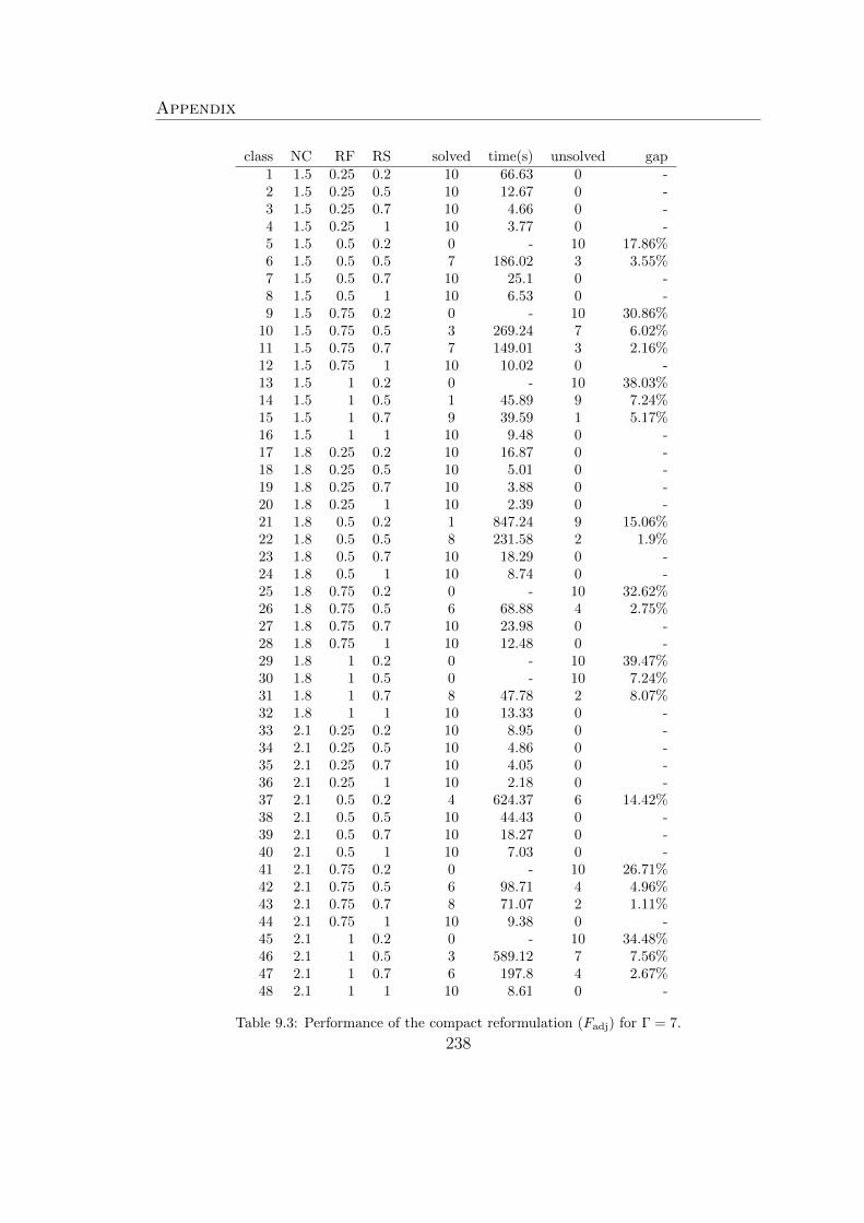
Appendix
class NC RF RS solved time(s) unsolved gap1 1.5 0.25 0.2 10 66.63 0 -2 1.5 0.25 0.5 10 12.67 0 -3 1.5 0.25 0.7 10 4.66 0 -4 1.5 0.25 1 10 3.77 0 -5 1.5 0.5 0.2 0 - 10 17.86%6 1.5 0.5 0.5 7 186.02 3 3.55%7 1.5 0.5 0.7 10 25.1 0 -8 1.5 0.5 1 10 6.53 0 -9 1.5 0.75 0.2 0 - 10 30.86%
10 1.5 0.75 0.5 3 269.24 7 6.02%11 1.5 0.75 0.7 7 149.01 3 2.16%12 1.5 0.75 1 10 10.02 0 -13 1.5 1 0.2 0 - 10 38.03%14 1.5 1 0.5 1 45.89 9 7.24%15 1.5 1 0.7 9 39.59 1 5.17%16 1.5 1 1 10 9.48 0 -17 1.8 0.25 0.2 10 16.87 0 -18 1.8 0.25 0.5 10 5.01 0 -19 1.8 0.25 0.7 10 3.88 0 -20 1.8 0.25 1 10 2.39 0 -21 1.8 0.5 0.2 1 847.24 9 15.06%22 1.8 0.5 0.5 8 231.58 2 1.9%23 1.8 0.5 0.7 10 18.29 0 -24 1.8 0.5 1 10 8.74 0 -25 1.8 0.75 0.2 0 - 10 32.62%26 1.8 0.75 0.5 6 68.88 4 2.75%27 1.8 0.75 0.7 10 23.98 0 -28 1.8 0.75 1 10 12.48 0 -29 1.8 1 0.2 0 - 10 39.47%30 1.8 1 0.5 0 - 10 7.24%31 1.8 1 0.7 8 47.78 2 8.07%32 1.8 1 1 10 13.33 0 -33 2.1 0.25 0.2 10 8.95 0 -34 2.1 0.25 0.5 10 4.86 0 -35 2.1 0.25 0.7 10 4.05 0 -36 2.1 0.25 1 10 2.18 0 -37 2.1 0.5 0.2 4 624.37 6 14.42%38 2.1 0.5 0.5 10 44.43 0 -39 2.1 0.5 0.7 10 18.27 0 -40 2.1 0.5 1 10 7.03 0 -41 2.1 0.75 0.2 0 - 10 26.71%42 2.1 0.75 0.5 6 98.71 4 4.96%43 2.1 0.75 0.7 8 71.07 2 1.11%44 2.1 0.75 1 10 9.38 0 -45 2.1 1 0.2 0 - 10 34.48%46 2.1 1 0.5 3 589.12 7 7.56%47 2.1 1 0.7 6 197.8 4 2.67%48 2.1 1 1 10 8.61 0 -
Table 9.3: Performance of the compact reformulation (Fadj) for Γ = 7.
238
Bibliography
V. Aggarwal, Y. P. Aneja, and K. P. K. Nair. Minimal spanning tree subject to aside constraint. Computers and Operations Research, 9(4):287–296, 1982.
R. K. Ahuja, T. L. Magnanti, and J. B. Orlin. Network Flows: Theory, Algorithms,and Applications. Prentice Hall, 1993.
H. Aissi, C. Bazgan, and D. Vanderpooten. Min-max and min-max regret ver-sions of combinatorial optimization problems: A survey. European Journal ofOperational Research, 197(2):427–438, 2009.
C. Artigues and F. Roubellat. A polynomial activity insertion algorithm in a multi-resource schedule with cumulative constraints and multiple modes. EuropeanJournal of Operational Research, 127(2):297–316, 2000.
C. Artigues, P. Michelon, and S. Reusser. Insertion techniques for static and dy-namic resource-constrained project scheduling. European Journal of OperationalResearch, 149(2):249–267, 2003.
C. Artigues, S. Demassey, and E. Neron. Resource-Constrained Project Scheduling:Models, Algorithms, Extensions and Applications. ISTE/Wiley, 2008.
C. Artigues, R. Leus, and F. T. Nobibon. Robust optimization for resource-constrained project scheduling with uncertain activity durations. Flexible Ser-vices and Manufacturing Journal, 25:175–205, 2013.
G. Ausiello, V. Bonifaci, and B. Escoffier. Complexity and Approximation inReoptimization. Preprint. https://hal.archives-ouvertes.fr/hal-00906941, 2008.
J. Ayoub and M. Poss. Decomposition for adjustable robust linear optimizationsubject to uncertainty polytope. Computational Management Science, 13(2):219–239, 2016.
E. Bampis, B. Escoffier, M. Lampis, and V. T. Paschos. Multistage matchings.In 16th Scandinavian Symposium and Workshops on Algorithm Theory, SWAT2018, June 18-20, 2018, Malmo, Sweden, pages 7:1–7:13, 2018.
239
Bibliography
A. Ben-Tal and A. Nemirovski. Robust convex optimization. Mathematics ofOperations Research, 23(4):769–805, 1998.
A. Ben-Tal, A. P. Goryashko, E. Guslitzer, and A. Nemirovski. Adjustable robustsolutions of uncertain linear programs. Mathematical Programming, 99(2):351–376, 2004.
A. Ben-Tal, O. E. Housni, and V. Goyal. A tractable approach for designing piece-wise affine policies in two-stage adjustable robust optimization. MathematicalProgramming, 182(1):57–102, 2020.
P. Bendotti, P. Chretienne, P. Fouilhoux, and A. Quilliot. Anchored reactiveand proactive solutions to the CPM-scheduling problem. European Journal ofOperational Research, 261(1):67–74, 2017.
P. Bendotti, P. Chretienne, P. Fouilhoux, and A. Pass-Lanneau. The Anchor-Robust Project Scheduling Problem. Preprint. https://hal.archives-ouvertes.fr/hal-02144834, 2019.
P. Bendotti, P. Chretienne, P. Fouilhoux, and A. Pass-Lanneau. Dominance-basedlinear formulation for the Anchor-Robust Project Scheduling Problem. Preprint.https://hal.archives-ouvertes.fr/hal-02938158, 2020a.
P. Bendotti, P. Chretienne, P. Fouilhoux, and A. Pass-Lanneau. Anchoredrescheduling problems under generalized precedence constraints. In M. Baıou,B. Gendron, O. Gunluk, and A. R. Mahjoub, editors, Combinatorial Optimiza-tion. ISCO 2020, volume 12176 of Lecture Notes in Computer Science, 2020b.
A. Berger, V. Bonifaci, F. Grandoni, and G. Schafer. Budgeted matching and bud-geted matroid intersection via the gasoline puzzle. Mathematical Programming,128:355–372, 2011.
D. Bertsimas and C. Caramanis. Finite adaptability in multistage linear optimiza-tion. IEEE Transactions on Automatic Control, 55(12):2751–2766, 2010.
D. Bertsimas and V. Goyal. On the power and limitations of affine policies intwo-stage adaptive optimization. Mathematical Programming, 134(2):491–531,2012.
D. Bertsimas and M. Sim. Robust discrete optimization and network flows. Math-ematical Programming, 98(1-3):49–71, 2003.
D. Bertsimas and M. Sim. The price of robustness. Operations Research, 52:35–53,2004.
240
Bibliography
D. Bienstock and N. Ozbay. Computing robust basestock levels. Discrete Opti-mization, 5(2):389–414, 2008.
A. Billionnet, M. Costa, and P. Poirion. 2-stage robust MILP with continuousrecourse variables. Discrete Applied Mathematics, 170:21–32, 2014.
J. R. Birge and F. Louveaux. Introduction to Stochastic Programming. Springer,2011.
H.-J. Bockenhauer, J. Hromkovic, T. Momke, and P. Widmayer. On the hardness ofreoptimization. In V. Geffert, J. Karhumaki, A. Bertoni, B. Preneel, P. Navrat,and M. Bielikova, editors, SOFSEM 2008: Theory and Practice of ComputerScience, pages 50–65. Springer, 2008.
M. Bold and M. Goerigk. A compact reformulation of the two-stage robustresource-constrained project scheduling problem. Preprint. https://arxiv.org/abs/2004.06547, 2020.
E. Boros, K. Borys, K. M. Elbassioni, V. Gurvich, and G. Rudolf. Inapproxima-bility bounds for shortest-path network interdiction problems. Technical report,Rutgers University, 2006.
M. Bruni, L. Di Puglia Pugliese, P. Beraldi, and F. Guerriero. An adjustable robustoptimization model for the resource-constrained project scheduling problem withuncertain activity durations. Omega, 71:66–84, 2017.
M. Bruni, L. Di Puglia Pugliese, P. Beraldi, and F. Guerriero. A computationalstudy of exact approaches for the adjustable robust resource-constrained projectscheduling problem. Computers and Operations Research, 99:178–190, 2018.
C. Buchheim and J. Kurtz. Robust combinatorial optimization under convex anddiscrete cost uncertainty. EURO Journal on Computational Optimization, 6(3):211–238, 2018.
C. Busing. Recoverable robust shortest path problems. Networks, 59(1):181–189,2012.
C. Busing, A. M. C. A. Koster, and M. Kutschka. Recoverable robust knapsacks:Γ-scenarios. In J. Pahl, T. Reiners, and S. Voß, editors, Network Optimization- 5th International Conference, INOC 2011, Hamburg, Germany, June 13-16,2011. Proceedings, volume 6701 of Lecture Notes in Computer Science, pages583–588. Springer, 2011.
K. Calhoun, R. Deckro, J. Moore, J. Chrissis, and J. Hove. Planning and re-planning in project and production scheduling. Omega, 30:155–170, 2002.
241
Bibliography
P. Chretienne. Reactive and proactive single-machine scheduling to maintain amaximum number of starting times. Annals of Operations Research, pages 1–14, 2018.
G. D’Angelo, G. Di Stefano, A. Navarra, and C. Pinotti. Recoverable robusttimetables: An algorithmic approach on trees. IEEE Transactions on Comput-ers, 60:433–446, 2011.
S. V. de Vonder, F. Ballestın, E. Demeulemeester, and W. Herroelen. Heuristicprocedures for reactive project scheduling. Computers and Industrial Engineer-ing, 52(1):11–28, 2007.
F. Deblaere, E. Demeulemeester, and W. Herroelen. Reactive scheduling in themulti-mode RCPSP. Computers and Operations Research, 38(1):63–74, 2011.
R. P. Dilworth. A decomposition theorem for partially ordered sets. Annals ofMathematics, 51(1):161–166, 1950.
J. R. Edmonds. Matroids and the greedy algorithm. Mathematical Programming,1(1):127–136, 1971.
G. N. Frederickson and R. Solis-Oba. Increasing the weight of minimum spanningtrees. Journal of Algorithms, 33(2):244–266, 1999.
V. Gabrel, M. Lacroix, C. Murat, and N. Remli. Robust location transportationproblems under uncertain demands. Discrete Applied Mathematics, 164:100–111,2014.
M. R. Garey and D. S. Johnson. Computers and Intractability: A Guide to theTheory of NP-Completeness. W. H. Freeman and Co., New York, NY, USA,1979.
A. Gupta, K. Talwar, and U. Wieder. Changing bases: Multistage optimization formatroids and matchings. In Automata, Languages, and Programming - 41st In-ternational Colloquium, ICALP 2014, Copenhagen, Denmark, July 8-11, 2014,Proceedings, Part I, pages 563–575, 2014.
H. W. Hamacher and G. Ruhe. On spanning tree problems with multiple objec-tives. Annals of Operations Research, 52:209–230, 1994.
G. A. Hanasusanto, D. Kuhn, and W. Wiesemann. K -adaptability in two-stagerobust binary programming. Operations Research, 63(4):877–891, 2015.
242
Bibliography
O. Hazır and G. Ulusoy. A classification and review of approaches and meth-ods for modeling uncertainty in projects. International Journal of ProductionEconomics, 223:107522, 2020.
W. Herroelen and R. Leus. Project scheduling under uncertainty: Survey andresearch potentials. European Journal of Operational Research, 165:289–306,2002.
W. Herroelen and R. Leus. The construction of stable project baseline schedules.European Journal of Operational Research, 156(3):550–565, 2004.
O. E. Housni and V. Goyal. On the optimality of affine policies for budgeteduncertainty sets. Preprint. https://arxiv.org/abs/1807.00163, 2019.
M. Hradovich, A. Kasperski, and P. Zielinski. Recoverable robust spanning treeproblem under interval uncertainty representations. Journal of CombinatorialOptimization, 34(2):554–573, 2017.
E. Israeli and R. K. Wood. Shortest-path network interdiction. Networks, 40(2):97–111, 2002.
A. Kasperski and P. Zielinski. Robust discrete optimization under discrete andinterval uncertainty: A survey. In M. Doumpos, C. Zopounidis, and E. Grig-oroudis, editors, Robustness Analysis in Decision Aiding, Optimization, andAnalytics, pages 113–143. Springer International Publishing, 2016.
A. Kasperski and P. Zielinski. Robust recoverable and two-stage selection prob-lems. Discrete Applied Mathematics, 233:52–64, 2017.
R. Kolisch and S. Hartmann. Heuristic algorithms for the resource-constrainedproject scheduling problem: Classification and computational analysis. InJ. Weglarz, editor, Project Scheduling: Recent Models, Algorithms and Applica-tions, pages 147–178. Springer US, Boston, MA, 1999.
R. Kolisch and A. Sprecher. PSPLIB – a project scheduling problem library.European Journal of Operational Research, 96:205–216, 1996.
O. Kone, C. Artigues, P. Lopez, and M. Mongeau. Comparison of mixed inte-ger linear programming models for the resource-constrained project schedulingproblem with consumption and production of resources. Flexible Services andManufacturing Journal, 25(1-2):24–47, 2013.
B. Korte and J. Vygen. Combinatorial Optimization: Theory and Algorithms.Springer Publishing Company, Incorporated, 5th edition, 2012.
243
Bibliography
P. Kouvelis and G. Yu. Robust Discrete Optimization and Its Applications.Springer, 1996.
S. Lendl, B. Peis, and V. Timmermans. Matroid bases with cardinality constraintson the intersection. Preprint. http://arxiv.org/abs/1907.04741, 2019.
C. Liebchen, M. Lubbecke, R. Mohring, and S. Stiller. The concept of recoverablerobustness, linear programming recovery, and railway applications. Robust andOnline Large-Scale Optimization, 5868:1–27, 2009.
M. Minoux. Models and algorithms for robust PERT scheduling with time-dependent task durations. Vietnam Journal of Mathematics, 35, 2007a.
M. Minoux. Duality, Robustness, and 2-stage robust LP decision models. Appli-cation to Robust PERT Scheduling. Annales du LAMSADE n.7, 2007b.
M. Minoux. Robust linear programming with right-hand-side uncertainty, dualityand applications. In Encyclopedia of Optimization, Second Edition, pages 3317–3327. 2009.
K. Mulmuley, U. V. Vazirani, and V. V. Vazirani. Matching is as easy as matrixinversion. Combinatorica, 7(1):105–113, 1987.
E. Nasrabadi and J. B. Orlin. Robust optimization with incremental recourse.Preprint. http://arxiv.org/abs/1312.4075, 2013.
C. H. Papadimitriou and M. Yannakakis. The complexity of restricted spanningtree problems. Journal of the ACM, 29(2):285–309, 1982.
A. Pass-Lanneau, P. Bendotti, and L. Brunod-Indrigo. Exact and heuristicmethods for Anchor-Robust and Adjustable-Robust RCPSP. Preprint. https://arxiv.org/abs/2011.02020, 2020.
M. Pinedo. Scheduling: Theory, Algorithms, and Systems. Springer, Boston, MA,4th edition, 2002.
R. Rahmaniani, T. G. Crainic, M. Gendreau, and W. Rei. The Benders decomposi-tion algorithm: A literature review. European Journal of Operational Research,259(3):801 – 817, 2017.
R. Ravi and M. X. Goemans. The constrained minimum spanning tree problem.In R. Karlsson and A. Lingas, editors, Algorithm Theory — SWAT’96, pages66–75. Springer Berlin Heidelberg, 1996.
244
Bibliography
H. Sakkout and M. Wallace. Probe backtrack search for minimal perturbation indynamic scheduling. Constraints, 5:359–388, 2000.
B. Schieber, H. Shachnai, G. Tamir, and T. Tamir. A theory and algorithms forcombinatorial reoptimization. Algorithmica, 80(2):576–607, 2018.
A. Schrijver. Combinatorial Optimization – Polyhedra and Efficiency. Springer-Verlag Berlin Heidelberg, 2003.
O. Seref, R. K. Ahuja, and J. B. Orlin. Incremental network optimization: Theoryand algorithms. Operations Research, 57(3):586–594, 2009.
S. F. Smith. Reactive Scheduling Systems, pages 155–192. Springer US, Boston,MA, 1995.
F. Sourd and O. Spanjaard. A multiobjective branch-and-bound framework: Ap-plication to the biobjective spanning tree problem. INFORMS Journal on Com-puting, 20(3):472–484, 2008.
A. L. Soyster. Technical note – convex programming with set-inclusive constraintsand applications to inexact linear programming. Operations Research, 21(5):1154–1157, 1973.
A. Subramanyam, C. E. Gounaris, and W. Wiesemann. K -adaptability in two-stage mixed-integer robust optimization. Mathematical Programming Computa-tion, 12(2):193–224, 2020.
J. Valdes, R. E. Tarjan, and E. L. Lawler. The recognition of series paralleldigraphs. SIAM Journal on Computing, 11(2):298–313, 1982.
T. Yi, K. G. Murty, and C. Spera. Matchings in colored bipartite networks.Discrete Applied Mathematics, 121(1):261 – 277, 2002.
R. Yuster. Almost exact matchings. Algorithmica, 63:39–50, 2012.
B. Zeng and L. Zhao. Solving two-stage robust optimization problems using acolumn-and-constraint generation method. Operations Research Letters, 41(5):457 – 461, 2013.
245


