Andersen_Kevin_MASc_2016.pdf - University of Victoria

Development of a Time-Domain Modeling Platform for Hybrid

Marine Propulsion Systems

by

Kevin Andersen

Bachelor of Engineering, University of Victoria, 2009

A Thesis Submitted in Partial Fulfillment

of the Requirements for the Degree of

MASTER OF APPLIED SCIENCE

in the Department of Mechanical Engineering

Kevin Andersen, 2016

University of Victoria

All rights reserved. This thesis may not be reproduced in whole or in part, by photocopy

or other means, without the permission of the author.

ii

Supervisory Committee

Development of a Time-Domain Modeling Platform for Hybrid

Marine Propulsion Systems

by

Kevin Andersen

Bachelor of Engineering, University of Victoria, 2009


Dr. Zuomin Dong, Department of Mechanical Engineering Supervisor

Dr. Bradley Buckham, Department of Mechanical Engineering Co-Supervisor

Dr. Peter Oshkai, Department of Mechanical Engineering Departmental Member

iii

Abstract


Dr. Zuomin Dong, Department of Mechanical Engineering Supervisor

Dr. Bradley Buckham, Department of Mechanical Engineering Co-Supervisor

Dr. Peter Oshkai, Department of Mechanical Engineering Departmental Member

This thesis develops a time-domain integrated modeling approach for design of hybrid-

electric marine propulsion systems that enables co-simulation of powertrain dynamics

along with ship hydrodynamics. This work illustrates the model-based design and analysis

methodology by performing a case study for an EV conversion of a short-cross ferry using

the BC Ferries’ M.V. Klitsa. A data acquisition study was performed to establish the typical

mission cycle of the ship for its crossing route between Brentwood Bay and Mill Bay,

across the Saanich Inlet near Victoria, BC Canada. The data provided by the data

acquisition study serves as the primary means of validation for the model’s ability to

accurately predict powertrain loads over the vessel’s standard crossing. This functionality

enables model-based powertrain and propulsion system design optimization through

simulation to intelligently deploy hybrid-electric propulsion architectures.

The ship dynamics model is developed using a Newton-Euler approach which

incorporates hydrodynamic coefficient data produced by potential flow solvers. The

radiation forces resulting from vessel motion are fit to continuous time-domain transfer

functions for computational efficiency. The ship resistance drag matrix is parameterized

using results from uRANS CFD studies that span the operating range of the vessel. A model

of the existing well-mounted azimuthing propeller is developed to predict thrust production

and mechanical torque for pseudo-second quadrant operation to represent all operating

conditions seen in real operation. The propeller model is parameterized from the results of

a series of uRANS CFD on the propeller geometry. A full battery-electric powertrain model

is produced to study the accuracy of the model in predicting the drivetrain loads, as well as

assessing the technological feasibility of an EV conversion for this particular vessel. A

dual-polarization equivalent circuit model is created for a large-scale LTO battery pack.

An average value model with MTPA control and dynamics loss model is developed for a

commercially available electric drive system. Power loss models were developed for

required converter topologies for computational efficiency. The model results for load

prediction are compared to data acquired, and results indicate that the approach is effective

for enabling the study of various powertrain architecture alternatives.

iv

Table of Contents

Supervisory Committee ...................................................................................................... ii

Abstract .............................................................................................................................. iii

Table of Contents ............................................................................................................... iv

List of Tables .................................................................................................................... vii

List of Figures .................................................................................................................. viii

Acknowledgments............................................................................................................. xii

Dedication ........................................................................................................................ xiii

Glossary of Acronyms and Abbreviations ....................................................................... xiv

Chapter 1 Introduction ..................................................................................................... 1

1.1 Research Motivations.......................................................................................... 1

1.2 Marine Hybridization and Electrification ........................................................... 4

1.3 Hybrid Vehicle Powertrain Development in the Automotive Industry .............. 6

1.4 Case Study – BC Ferries M.V. Klitsa ................................................................. 9

1.5 Related Work and Literature Review ............................................................... 12

1.5.1 Integrated Power System Modeling for Hybrid Marine Propulsion ............. 13

1.5.2 Hybrid Electric Vehicle Technology ............................................................ 15

1.5.3 Thruster Dynamics Modeling ....................................................................... 19

1.5.4 Vessel Dynamics Modeling – Maneuvering and Seakeeping ....................... 20

1.6 Thesis Roadmap ................................................................................................ 22

1.7 Research Contributions ..................................................................................... 24

Chapter 2 Ship Propulsion Modeling and Dynamics .................................................... 27

2.1 Ship Propulsion – An Introduction ................................................................... 28

2.1.1 Propeller Efficiency ...................................................................................... 30

2.1.2 Mechanical Transmission Chain ................................................................... 31

2.1.3 Propeller Dynamics and Performance Modeling .......................................... 34

2.2 Hybrid-Electric Integrated Power Systems Modeling ...................................... 42

2.2.1 Battery Energy Storage System Modeling .................................................... 44

2.2.2 Variable Speed PMSM Electric Drive System ............................................. 49

2.2.3 Power Converter Modeling ........................................................................... 57

2.2.4 Lithium-Ion Battery Rapid Charging ............................................................ 59

2.3 Vessel Dynamics Modeling .............................................................................. 61

2.3.1 Ship Dynamics Modeling ............................................................................. 61

2.3.2 Coordinate System Definitions and Notation ............................................... 62

2.3.3 Seakeeping Analysis and the Classical Frequency-Domain Model ............. 65

2.3.4 Unified Seakeeping/Maneuvering Analyses for Vessel Dynamics Model ... 68

2.3.5 Formulation of Ship Resistance .................................................................... 71

2.3.6 Evaluation of the Fluid-Memory Effects ...................................................... 76

2.3.7 Integration of ShipMo3D with Marine Systems Simulation Toolbox .......... 81

v

2.4 Integrated Modeling – Assembling the Pieces for Study of Hybrid Electric

Propulsion ......................................................................................................... 81

Chapter 3 Development of an Azimuthing Propeller Model for Integrated Powertrain

Simulations ................................................................................................... 86

3.1 Model Development Methodology ................................................................... 86

3.1.1 Thruster Geometry ........................................................................................ 87

3.2 Quadrants of Operation and Off-Design Conditions ........................................ 89

3.3 CFD Design of Experiment and Lookup Table Generation ............................. 92

3.4 Development of Simulink-Based Thrust Model and Validation .................... 101

3.4.1 Thruster Configuration and Vessel Actuation Forces for M.V. Klitsa ....... 104

Chapter 4 Development of a Time-Domain Dynamics Model for a Barge-Type Ferry

Hull ............................................................................................................. 106

4.1 Development of Ship Inertial Model .............................................................. 106

4.1.1 Generation of Hydrodynamic Coefficients Data ........................................ 110

4.1.2 Vessel Dynamics Model ............................................................................. 115

4.1.3 Construction of Drag Matrix ....................................................................... 117

4.1.4 Radiation and Diffraction Forces and Wave Excitation ............................. 122

4.1.5 Wake Fraction and Thrust Deduction Factors ............................................ 129

Chapter 5 Modeling of AES Power System ................................................................ 133

5.1 Model Fidelity of Hybrid Power Systems ...................................................... 133

5.2 Proposed Architecture ..................................................................................... 134

5.2.1 Battery Modeling ........................................................................................ 136

5.2.2 Bi-Directional DC/DC Converter Modeling ............................................... 147

5.2.3 Permanent Magnet Synchronous Machine Electric Drive System ............. 160

5.2.4 Rapid-Charge Infrastructure ....................................................................... 178

5.2.5 Islanding Converter for Hotel Loads .......................................................... 183

Chapter 6 Summary of M.V. Klitsa Data Acquisition Experiment and Load Profile

Generation ................................................................................................... 184

6.1 Introduction to Data Acquisition Experiment ................................................. 184

6.2 Development of Load Profiles from Operational Data ................................... 187

6.3 Comparison of Vessel Course for Validation of Dynamics Model ................ 194

6.4 Experimental Uncertainties ............................................................................. 196

6.4.1 Environmental Errors .................................................................................. 197

6.4.2 ECM Measurement Errors .......................................................................... 200

6.4.3 Signal Noise in Engine Signals ................................................................... 200

Chapter 7 System Model Validation and Simulation Results ..................................... 201

7.1 System Model Implementation ....................................................................... 202

7.2 Powertrain Load Prediction and Verification ................................................. 206

7.2.1 Simulation Results for Different Load Profiles .......................................... 206

7.2.2 BEIPS Performance Results ....................................................................... 212

vi

7.3 Simulation Results Including Vessel Dynamics ............................................. 214

7.4 Analysis and Discussion of Results ................................................................ 219

7.4.1 Model vs. Experimental Direct Comparison .............................................. 219

7.4.2 Model and Sub-System Uncertainties ......................................................... 221

Chapter 8 Conclusions and Recommendations ........................................................... 227

8.1 General Summary and Conclusions ................................................................ 227

8.2 Summary of Recommendations ...................................................................... 230

8.2.1 Additional Experimentation ........................................................................ 231

8.2.2 PTO and Rotational Damping model .......................................................... 232

8.2.3 Refinement of Inertial Properties ................................................................ 233

8.2.4 Vector Decomposition of GPS Speed Data ................................................ 233

8.2.5 Thrust Deduction Factor Parameterization ................................................. 234

8.3 Concluding Remarks ....................................................................................... 234

Bibliography ................................................................................................................... 236

Appendix A - Data Acquisition Experiment ................................................................... 242

Appendix B – Derivation of DC/DC Converter Control Law ........................................ 281

Appendix C – IGBT Datasheet for Loss Model ............................................................. 289

vii

List of Tables

Table 1: Charging Availability under Current Operating Schedule ................................. 11

Table 2: Time Constants of AES Ship Subsystems [14] .................................................. 43

Table 3: Retardation Function Characteristics for Transfer Function Fitting................... 80

Table 4: Operating Points used for Oblique Flow CFD Analyses .................................. 100

Table 5: CFD Results for Angled Flow .......................................................................... 100

Table 6: Summary of Propeller System Model Parameters ............................................ 104

Table 7: Normal Departure Parameters from the Stability Book [94] and Comparison

with CAD Model Estimate.............................................................................................. 109

Table 8: Assumed Parameters for Centre of Gravity Location and Vessel Draft ........... 110

Table 9: Inertial Data for Hydrodynamic Coefficient Generation .................................. 110

Table 10: Fitted Parameters using Least Squared Fitting with Genetic Algorithm ........ 119

Table 11: Assumed Parameters for Viscous Damping Matrix Coefficients ................... 121

Table 12: Parameters for Numerical Integration of Non-Linear Drag Forces in Sway and

Yaw ................................................................................................................................. 122

Table 13: Computation of Thrust Deduction Factor from Operational Data.................. 131

Table 14: Installed Capacity of Primary Equipment Onboard M.V. Klitsa.................... 136

Table 15: Summary of Equivalent Circuit Parameters for 9.2kWh Module .................. 140

Table 16: First-Pass Design Requirements for Power Output ........................................ 142

Table 17: First-Pass Design for ESS Capacity Estimation ............................................. 142

Table 18: Single 9.2kWh Module Technical Specifications .......................................... 143

Table 19: Battery Pack Configuration and Specifications .............................................. 143

Table 20: Desired Control Law BEIPS ........................................................................... 149

Table 21: Small-signal Approximation Equations for Controller Development ............ 153

Table 22: HVDC Control Transfer Function for Buck and Boost Mode ....................... 153

Table 23: Low and High Load Comparison for M.V. Klitsa with Single Converter ..... 155

Table 24: Low and High Load Comparison of M.V. Klitsa with Two Converters ........ 156

Table 25: Comparison of Diesel Engine Output with PMSM Electric Drive................. 160

Table 26: Motor Parameters for Simulation Model ........................................................ 162

Table 27: Estimated Motor Nameplate Data .................................................................. 163

Table 28: IGBT Parameters for Loss Estimation ............................................................ 164

Table 29: Charging System Capacity Sizing .................................................................. 179

Table 30: Summary of Acquired Parameters in Data Acquisition Study ....................... 185

Table 31: Potential Energy Savings from Zero-Speed Propeller Operation In-Berth .... 211

Table 32: Instantaneous Relative Error Analysis of Simulation Results ........................ 220

Table 33: Relative Modeling Uncertainty and Degree of Confidence ........................... 222

Table 34: Energy Consumption Results and Relative Error Against Experimental ....... 229

viii

List of Figures

Figure 1: Typical Diesel-Electric Conversion Losses [1] ................................................... 2

Figure 2: EPA Urban Dynamometer Driving Schedule [5] ................................................ 7

Figure 3: V-Diagram for Integrated System Development [6] ........................................... 8

Figure 4: M.V. Klitsa Operating Route and Schedule ...................................................... 10

Figure 5: Proposed BEIPS Architecture ........................................................................... 12

Figure 6: Illustration of Parallel Drive Gearbox (Top) and Right Angle Gearbox (Bottom)

Configurations................................................................................................................... 32

Figure 7: Propulsion Efficiency Breakdown for Traditional Diesel Propulsion [4] ......... 34

Figure 8: Traditional Definition of Propeller Quadrants .................................................. 36

Figure 9: Expansion of 4-Quadrant Definition to Represent Azimuthing Propellers ....... 37

Figure 10: Thevenin-Based Electrical Battery Circuit...................................................... 46

Figure 11: Impedance-Based Electrical Battery Circuit ................................................... 46

Figure 12: PMSM Equivalent Circuit including Iron Loss ............................................... 51

Figure 13: Inverter/Motor Topology ................................................................................. 53

Figure 14: Space Vector Diagram..................................................................................... 53

Figure 15: PMSM Drive AVM Block Diagram ............................................................... 57

Figure 16: Power Loss Model for Converters................................................................... 59

Figure 17: Cell Voltage as a Function of Charge Rate ..................................................... 60

Figure 18: Traditional Ship Resistance Decomposition in Calm Water [51] ................... 71

Figure 19: Simulation Platform Integration Methodology and Parameterization Strategy

........................................................................................................................................... 84

Figure 20: 2D Blade Profiles ............................................................................................ 89

Figure 21: 3D Wrapping of 2D sections ........................................................................... 89

Figure 22: 3D Propeller Geometry ................................................................................... 89

Figure 23: Propeller and 19A Duct ................................................................................... 89

Figure 24: Azimuth Propeller 1st Quadrant (left) and Pseudo 2nd Quadrant (right) .......... 90

Figure 25: Top-level Lookup Table Block Diagram ........................................................ 91

Figure 26: Comparison of KT and KQ CFD Predictions with Open-Water Published Data

........................................................................................................................................... 92

Figure 27: CFD Image Showing Velocity Magnitude Profile in 1st Quadrant ................. 94

Figure 28: Anti-Directional Flow Field from CFD........................................................... 95

Figure 29: Anti-Directional Velocity Magnitude from CFD ............................................ 95

Figure 30: Vague-Directional Flow Field from CFD ....................................................... 96

Figure 31: Vague-Directional Velocity Magnitude from CFD......................................... 96

Figure 32: Thrust and Torque Coefficient for Pseudo-Second Quadrant Results from CFD

........................................................................................................................................... 98

Figure 33: Top-Level Propeller Model Implementation in Simulink ............................. 102

Figure 34: Thrust Coefficient Lookup Surface (Produced by CFD) .............................. 103

ix

Figure 35: Torque Coefficient Lookup Surface (Produced by CFD) ............................. 103

Figure 36: Thruster Configuration on the M.V. Klitsa ................................................... 104

Figure 37: Thruster Inflow Conditions Resulting From Vessel Motions ....................... 105

Figure 38: Cross-Sectional View Illustrating Transverse Support Structure .................. 107

Figure 39: Crossing Sectional View Illustrating Longitudinal Support Structure .......... 107

Figure 40: 3D CAD Image of the Klitsa Used to Determine Inertial Properties ............ 109

Figure 41: Workflow for Parameterization of Vessel Models in the MSS Toolbox ...... 111

Figure 42: Panelled Hull in ShipMo3D .......................................................................... 112

Figure 43: Non-Dimensionalized Added Mass and Damping Coefficients Computed

using SM3D .................................................................................................................... 113

Figure 44: Historical Data of Significant Wave Height from Pat Bay Monitoring Buoy

(C46134) [95].................................................................................................................. 114

Figure 45: Final BuildShip Configuration for Computing Ship Hydrodynamic

Coefficients ..................................................................................................................... 115

Figure 46: Implementation of the Unified Seakeeping/Maneuvering Model [78] ......... 117

Figure 47: Comparison of Surge System Fitted Parameters ........................................... 119

Figure 48: Example of Transfer Function Fitting to Hydrodynamic Data in DOF (1,1) 124

Figure 49: Comparison of Kernel Function with Impulse Response of SS System (Surge)

......................................................................................................................................... 125

Figure 50: Comparison of Kernel Function with Impulse Response of SS System (Sway)

......................................................................................................................................... 126

Figure 51: Comparison of Kernel Function with Impulse Response of SS System (Heave)

......................................................................................................................................... 126

Figure 52: Comparison of Kernel Function with Impulse Response of SS System (Roll)

......................................................................................................................................... 127

Figure 53: Comparison of Kernel Function with Impulse Response of SS System (Pitch)

......................................................................................................................................... 127

Figure 54: Comparison of Kernel Function with Impulse Response of SS System (Yaw)

......................................................................................................................................... 128

Figure 55: Plot of Wake Fraction as Function of Ship Speed......................................... 129

Figure 56: Plot of Thrust Deduction versus Forward Speed........................................... 131

Figure 57: Thrust Deduction Dynamic Model Implementation ..................................... 132

Figure 58: Dual Polarization Circuit ............................................................................... 137

Figure 59: Construction of Large-Scale Battery Model Using Module Test Data ......... 138

Figure 60: Comparison of Battery Model and Results from [43] ................................... 141

Figure 61: Construction of Battery Pack from Module Blocks in Simulink using

Simscape ......................................................................................................................... 144

Figure 62: 1C Discharge Test for 3S60P Module Battery Pack to Confirm Capacity ... 145

Figure 63: Response Comparison of Fitted Simulink Model versus Simscape Model .. 146

Figure 64: SOC Comparison of Fitted Simulink Model versus Simscape Model .......... 146

x

Figure 65: Bi-Directional Buck-Boost Converter Topology for Ship Applications ....... 148

Figure 66: Gate Signal Pattern for Bi-Directional DC/DC Converter for Boost Mode [25]

......................................................................................................................................... 150

Figure 67: Gate Signal Pattern for Bi-Directional DC/DC Converter for Buck Mode .. 152

Figure 68: Efficiency Curve of Commercially Available 200kW Bi-Directional

Buck/Boost Converter [98] ............................................................................................. 154

Figure 69: Implementation of Power Loss Model in Using Simscape ........................... 157

Figure 70: DC-DC Converter Model Operating in Boost Mode .................................... 158

Figure 71: DC-DC Converter Model Operating in Buck Mode ..................................... 159

Figure 72: Average Value Model Implementation for Electric Drive System ............... 161

Figure 73: Peak and Continuous Power Outputs for the Electric Drive System ............ 163

Figure 74: Current Splitting using Multiple Parallel Switching Devices ....................... 165

Figure 75: Implementation of Analytical Semiconductor Dynamic Loss Model for VSI

......................................................................................................................................... 165

Figure 76: Control System Block Diagram .................................................................... 166

Figure 77: Procedure for Generating MTPA Lookup Tables ......................................... 168

Figure 78: Plot of MTPA Id Reference Lookup Data ...................................................... 169

Figure 79: Plot of MTPA Iq Reference Lookup Data ..................................................... 169

Figure 80: Step Response of Electric Drive System with Speed Control ....................... 170

Figure 81: Published Motor Efficiency Map .................................................................. 171

Figure 82: Comparison of First Principles Loss Model with Published Data ................ 173

Figure 83: Top-Level Electric Drive System AVM Model Implementation in Simulink

......................................................................................................................................... 174

Figure 84: Top-Level Simulation Model for Motor Model ............................................ 174

Figure 85: Response Comparison of PMSM/Drive AVM versus Detailed Simulation

Model .............................................................................................................................. 176

Figure 86: Comparison of D-Q, DC Currents for PMSM/Drive AVM versus Detailed

Model .............................................................................................................................. 177

Figure 87: Comparison of DC Current for PMSM/Drive AVM and Detailed Model .... 178

Figure 88: Charger Model Implementation in Simulink................................................. 180

Figure 89: Rapid Charger State Machine Logic ............................................................. 180

Figure 90: Fast Charging Performance of the Battery and Charger at 5C ...................... 181

Figure 91: Regular Charging Performance of the Battery and Charger at 1C ................ 182

Figure 92: DC/AC Converter Approximation Model Implementation ........................... 183

Figure 93: CAN Network Schematic and General Arrangement for DAQ Study .......... 186

Figure 94: Plot of Ship Speed vs. Time for 3 Load Profiles ........................................... 188

Figure 95: Engine Speed Profiles ................................................................................... 189

Figure 96: Engine Load Profiles ..................................................................................... 190

Figure 97: Example of Torque Transient during Azimuth Thruster Rotation ................ 191

Figure 98: Azimuth Angle Profiles ................................................................................. 192

xi

Figure 99: Plot of All Electrical Load Data Collected for Computation of the Mean .... 193

Figure 100: Plot of Representative Electrical Loads for High, Medium, and Low

Conditions ....................................................................................................................... 194

Figure 101: Plot of Course and Heading Data for the Three Load Profiles ................... 195

Figure 102: Travel Direction Definitions ....................................................................... 196

Figure 103: Historic Data for Computed Ocean Current Magnitude in Saanich Inlet [100]

......................................................................................................................................... 198

Figure 104: Approximate Current Heading from Ocean Networks Canada versus

Brentwood Bay – Mill Bay Crossing [101] .................................................................... 199

Figure 105: Propulsion System Model Implementation ................................................. 203

Figure 106: Electric Motor and Thruster Model Connections and Information Flow .... 203

Figure 107: Propeller and Vessel Dynamics Model Information Flow .......................... 204

Figure 108: Integrated Power System Model Implementation and Information Flow ... 204

Figure 109: Wake Fraction Generator Sub-System ........................................................ 205

Figure 110: Implementation of Velocity Source Selector .............................................. 205

Figure 111: Simulation Results for Load Profile 1 with Vessel Speed Specified .......... 208



Figure 114: SOC Discharge/Charge Profile for Rapid-Charge System .......................... 212

Figure 115: Plot of Component Efficiencies during Load Profiles ................................ 214

Figure 116: Simulation Results for Load Profile 1 including Vessel Dynamics ............ 215



xii

Acknowledgments

I would like to extend a huge debt of gratitude to my supervisor Dr. Zuomin Dong with

the supporting cast of Dr. Brad Buckham and Dr. Peter Oshkai for their guidance and

support throughout my time at UVic. I would also like to acknowledge the tireless efforts

of my colleague Mostafa Rahimpour who was instrumental in developing the necessary

information for me to complete my work.

I would also like to acknowledge the extensive support that we have received from

Bruce Paterson, Bob Kearney, Bambino Da Silva, and many other wonderful people at

BC Ferries who made this project possible. Their contributions, along with those from

many other industrial collaborators, were instrumental in supporting our research

activities, in particular with the work presented here.

Financial support to UVic’s Green Ship Hybrid Electric Propulsion System Modeling,

Design, and Control Optimization Tools project was provided by Transport Canada under

the Clean Transportation Initiative and the assistance from Ms. Marie-Chantal Ross,

Development Officer, CEESAR of Transport Canada are gratefully acknowledged.

xiii

Dedication

This thesis is dedicated to my dear fiancé Samantha Wilde for her relentless patience

and continuous support on the roller coaster of highs and lows that embodied this degree.

Her unwavering encouragement is the primary reason that I was able to complete this

thesis, for which I am eternally grateful.

I would also like to dedicate this to the loving memory of my late mother Diane

Andersen and late grandmother Helen Boyce, two women whom I adored and whose love

and strength inspired me to persevere in achieving my goals.

xiv

Glossary of Acronyms and Abbreviations

AC - Alternating Current

AC/DC - Alternating Current to Direct Current

AES - All Electric Ship

AVM - Average Value Model

BCF - BC Ferries

BEIPS - Battery Electric Integrated Power System

BEV - Battery Electric Vehicle

CAN - Controller Area Network

CC - Constant Current

CFD - Computational Fluid Dynamics

CV - Constant Voltage

DAQ - Data Acquisition

DC - Direct Current

DC/AC - Direct Current to Alternating Current

DC/DC - Direct Current to Direct Current

DoD - Depth of Discharge

DOF - Degree of Freedom

ECM - Engine Control Module

EMF - Electromotive Force

ESR - Equivalent Series Resistance

ESS - Energy Storage System

EV - Electric Vehicle

FCEV - Fuel Cell Electric Vehicle

FEM - Finite Element Modeling

GHG - Greenhouse Gas

GPS - Global Positioning System

HEV - Hybrid Electric Vehicle

HIL - Hardware-in-the-Loop

HPPC - Hybrid Pulsed Power Characterization

xv

ICE - Internal Combustion Engine

IMO - International Maritime Organization

IPS - Integrated Power System

Li-ion - Lithium Ion

LNG - Liquefied Natural Gas

LTO - Lithium Titanate Oxide

MARPOL - Short for Marine Pollution (Regulation acronym from IMO)

MBD - Model Based Design

MSS - Marine System Simulator

MTPA - Maximum Torque Per Ampere

NED - North East Down (Coordinate System Reference)

OCV - Open Circuit Voltage

OpEx - Operating Expense

PID - Proportional Integral Derivative (Controller)

PMM - Planar Motion Mechanism

PMSM - Permanent Magnet Synchronous Machine

PSAT - Powertrain Systems Analysis Toolkit

PTI - Power Take-In

PTO - Power Take-Off

RC - Resistor/Capacitor

SIL - Software-in-the-Loop

SOC - State of Charge

SQP - Sequential Quadratic Programming

uRANS - Unsteady Reynolds Averaged Navier-Stokes

VERES - Software Program short for VEssel RESponse

Chapter 1 Introduction

1.1 Research Motivations

Marine transportation has been a cornerstone of the great human civilizations

throughout history enabling expansion of trade, exploration of new territories, and

transportation of goods. Over the years marine vessels have evolved to meet the growing

demands of both trade and human transportation, driving the need for more efficient and

effective propulsion solutions. With the emphasis on delivering fast, inexpensive,

reliable, and safe marine transportation, propulsion systems has evolved drastically over

the last 300 years from its humble beginnings using human or wind power. Wind

powered sailing vessels were replaced by steamships, which enabled more reliable and

faster operation. Steamships were eventually replaced by diesel engines in the early-20th

century to minimize crew requirements, lower cost, and increase reliability in comparison

to steam engines.

In general, the traditional diesel propulsion power plant has been the standard

architecture for most vessels over the last 50 years; however, growing environmental

concerns and new emissions regulations imposed by the IMO are causing a major shift in

the industry’s approach to propulsion system design. Recent history excluded, the

escalating cost of oil provided the incentive to investigate more efficient and

technologically advanced architectures to reduce operational expenses (OpEx). Though

many diesel engine manufacturers are focusing their efforts on after-treatment systems to

comply with the MARPOL emission regulations, the industry has collectively been

exploring other opportunities for energy savings and emissions control which range from

2

burning cleaner fuels, such as LNG, to increasing the level of hybridization through more

electrification.

Diesel-electric hybrid ships have long been deployed in special application where the

vessel’s mission cycles are dynamic. Diesel electric ships can offer increased operational

efficiency when the power demand varies significantly. This performance gain is enabled

by an array of diesel generators that can be systematically brought online to best match

the generation to the active load, thus allowing generators to operate in higher efficiency

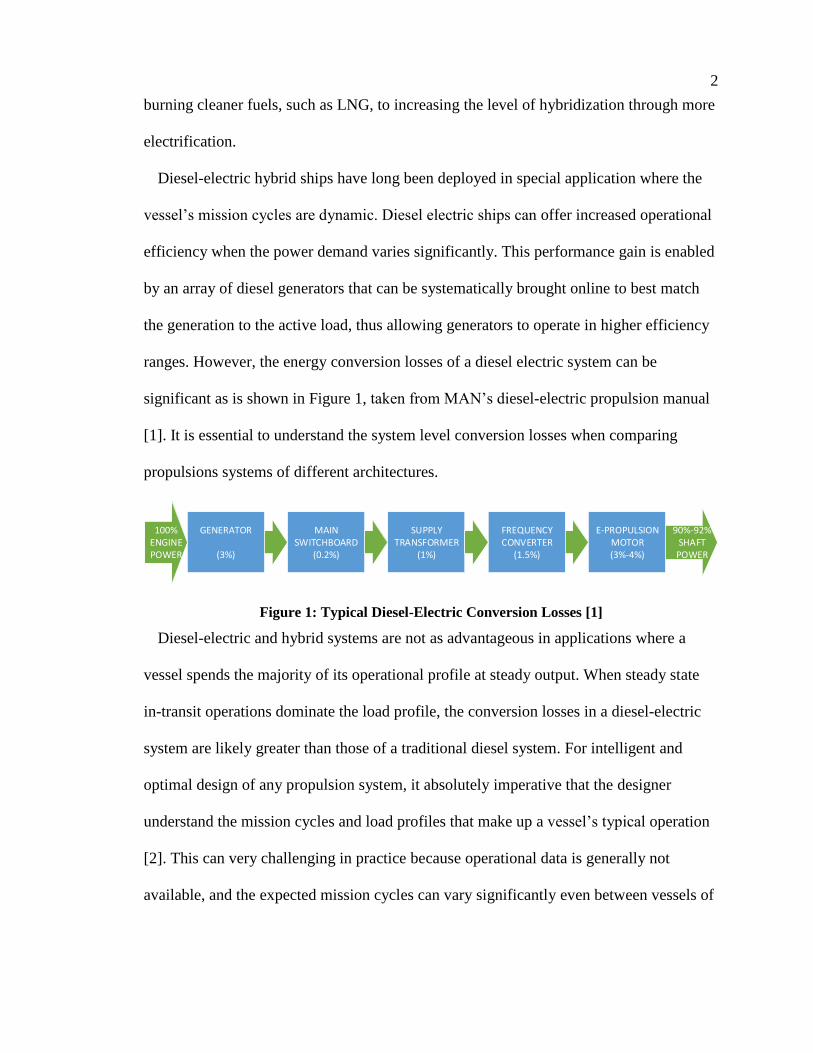
ranges. However, the energy conversion losses of a diesel electric system can be

significant as is shown in Figure 1, taken from MAN’s diesel-electric propulsion manual

[1]. It is essential to understand the system level conversion losses when comparing

propulsions systems of different architectures.

GENERATOR

(3%)

100% ENGINE POWER

MAIN SWITCHBOARD

(0.2%)

SUPPLY TRANSFORMER

(1%)

FREQUENCY CONVERTER

(1.5%)

E-PROPULSION MOTOR (3%-4%)

90%-92% SHAFT

POWER

Figure 1: Typical Diesel-Electric Conversion Losses [1]

Diesel-electric and hybrid systems are not as advantageous in applications where a

vessel spends the majority of its operational profile at steady output. When steady state

in-transit operations dominate the load profile, the conversion losses in a diesel-electric

system are likely greater than those of a traditional diesel system. For intelligent and

optimal design of any propulsion system, it absolutely imperative that the designer

understand the mission cycles and load profiles that make up a vessel’s typical operation

[2]. This can very challenging in practice because operational data is generally not

available, and the expected mission cycles can vary significantly even between vessels of

3

the same class. There are no standardized drivecycles that can be applied to marine

vessels, like those used in the automotive industry.

The ability to predict the ship’s load profile in the design stage, and the capability to

analyze the ship’s performance through time-domain dynamic simulation provides the

major motivating factors for this work. By creating a Model-in-the-Loop (MIL) platform

that is capable of representing the integrated power system (IPS) dynamics, along with

the hydrodynamics of thrust production and vessel motion, this work allows for advanced

propulsion systems to be simulated and numerically optimized to produce the best

possible system performance that meets the contract requirements. It also allows for

execution of Model Based Design (MBD) for development of the main supervisory

controller, enabling integrated controller synthesis for advanced energy management

systems. By using Matlab/Simulink, the platform can seamlessly be extended to

Software-in-the-Loop (SIL) and Hardware-in-the-Loop (HIL) to complete a vertically

integrated suite of development tools.

The MBD approach is the state-of-the-art design process used by the automotive and

aerospace industries, both industries realizing significant performance gains through

increased levels of integration using embedded systems. Embedded systems have the

ability to provide multi-variate and robust control for complex power systems, and are

essential for modern “smart” energy management system deployment. The marine sector

has, in many respects, lagged behind in adopting modern model-based design practices

for propulsion system design; therefore, this work sought to not only develop the

platform and methodology, but to also illustrate its effectiveness using a case study.

4

Lastly, there is a growing interest in introducing onboard energy storage and renewable

technologies into the IPS, which inherently requires a higher level of sophistication and

system integration. The MIL platform offers a method by which these technologies can

be evaluated through simulation, and systematically implemented through MBD to lower

risk and assist with economic projections.

1.2 Marine Hybridization and Electrification

The growth of the global fleet of electric and hybrid ships has outpaced traditional

diesel installations by a factor of three over the last ten years [2]. Electric and hybrid

propulsion offers more operational flexibility, and can achieve a significantly higher

conversion efficiency in compared to traditional diesel. Generally speaking, electric

drives achieve greater than 95% efficiency when operating between 5%-100% rated

power output. Contrast that to diesel engines, whose efficiency is highest in the

concentrated operating range of 85% - 90% rated power output [2]. When electric

propulsion is employed, the electrical energy is provided by a set of diesel generators that

can be brought online as needed to meet the load. By using multiple diesel generators

rated at a fraction of the ship’s maximum power demand, the energy conversion

efficiency of the system can be increased by managing the number of generators online

such that the internal combustion engine operates closer to peak efficiency.

The electric ship concept has proven to be highly effective in many commercial

applications including icebreakers, cruise ships, ferries, specialty precision vessels, ocean

service vessel, and drilling vessels [2]. Future trends in hybrid and electric propulsion

systems are leading to more flexible and integrated systems that include,

5

Parallel propeller drive systems that include PTO/PTI

Inclusion of energy storage

Moving from AC distribution to DC distribution grid

Full battery-electric or zero emission operation

A full-electric battery powered ferry named the Ampere, with 120 car and 360

passenger capacity, has recently entered service in Norway’s Sognefjord and has proven

that battery technology can be the sole power source for larger vessels [3]. Hybridized

vessels that include an energy storage system (ESS) enable several operational

advantages which are discussed by Hansen and Wendt in [2]. First, energy storage

provides a buffer bank that minimizes the requirements for spinning reserves; therefore,

fewer diesel gensets are required to be online. The energy buffer also allows for peak

shaving such that the generator equipment only services the average load. With sufficient

capacity, the ship can be operated in zero emission mode while in the harbour, or quiet

mode for noise sensitive applications.

Adoption of the DC grid allows for easier integration of alternative energy technologies

such as ultracapacitors, batteries, and fuel cells. It also eliminates the need for fixed speed

AC electricity generation. By removing the fixed-speed generator constraint required to

regulate the AC electrical frequency, it allows for highly efficient variable-speed

generation where the engine can now operate at its optimal torque-speed condition for a

given load. This naturally opens more opportunities for real-time energy management.

From an equipment layout perspective, the All Electric Ship (AES) offers more

flexibility in the placement of primary power plant equipment. When the internal

combustion prime movers no longer need to be mechanically coupled to the propellers,

6

the main and auxiliary generators can be placed at more convenient locations in the ship

allowing designers to better control noise emission and vibration. These are two areas

that are becoming of increased environmental concern for both human passengers/crew

and marine life [4].

The additional generators, electric motors, distribution systems, and converters may

carry increased cost over conventional installations; however, this is typically recovered

by fuel savings associated with the increased system efficiency [2], [4]. As mentioned

previously, the total efficiency when accounting for electrical losses from prime mover to

propulsor may be less than the traditional diesel system for certain applications [4];

therefore, it is of the utmost importance that the operating profiles be well understood in

the design phase.

1.3 Hybrid Vehicle Powertrain Development in the Automotive Industry

Hybrid electric vehicles (HEVs) and other variants have achieved excellent commercial

success in the automotive industry over the last ten years. Modern HEVs are highly

integrated embedded systems designed for robust control and real-time energy

management, even under highly dynamic operating profiles. Standard automotive

drivecycles, created to represent normal drive usage patterns, provide a metric of

comparison and a means of optimization for the vehicle in the design stage. The EPA

uses a series of these drivecycles to provide a standard dynamometer test procedure for

computing fuel economy ratings in consumer vehicles. An example of such a drivecycle

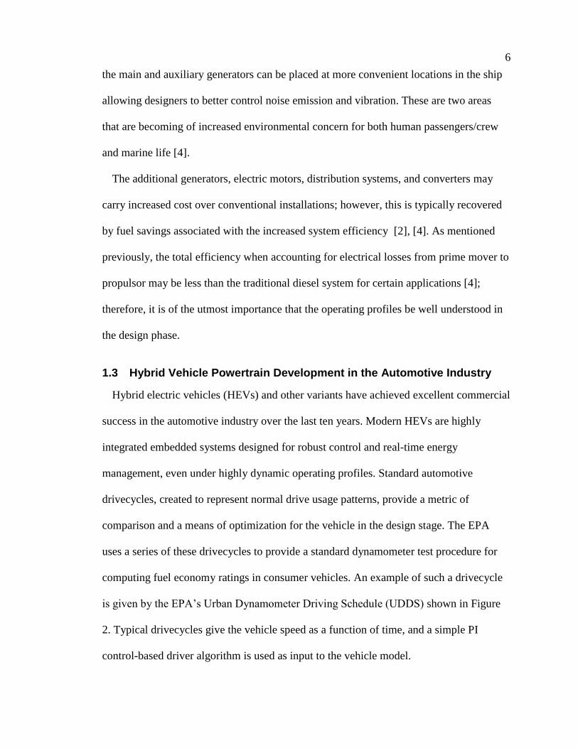
is given by the EPA’s Urban Dynamometer Driving Schedule (UDDS) shown in Figure

2. Typical drivecycles give the vehicle speed as a function of time, and a simple PI

control-based driver algorithm is used as input to the vehicle model.

7

Figure 2: EPA Urban Dynamometer Driving Schedule [5]

Automotive powertrain development is performed using the MBD strategy, where

time-domain models are systematically used throughout the design process to predict and

validate the vehicle’s performance. This approach generally includes,

1. Rapid numerical simulation of the vehicle’s performance in the design stage

using simplified power loss models for high level architectural studies

2. Detailed system simulation, analysis, optimization and validation using

Software-in-the-Loop development

3. Seamless integration of controller hardware for Hardware-in-the-Loop testing

using rapid prototyping and automatic code generation.

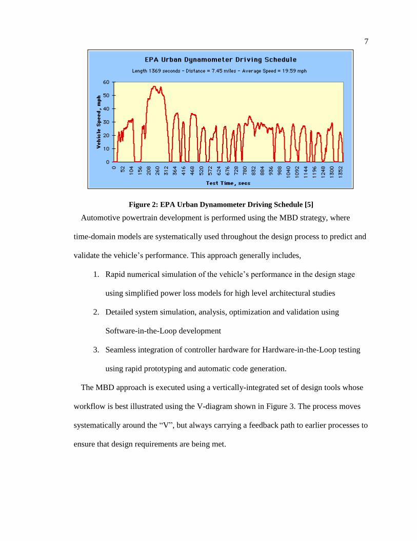
The MBD approach is executed using a vertically-integrated set of design tools whose

workflow is best illustrated using the V-diagram shown in Figure 3. The process moves

systematically around the “V”, but always carrying a feedback path to earlier processes to

ensure that design requirements are being met.

8

Figure 3: V-Diagram for Integrated System Development [6]

In this work, we are interested in developing a framework that can be applied to

advanced hybrid electric marine propulsion using the V-diagram approach. Modeling is

carried out using Matlab/Simulink as the base simulation software, and we develop a set

of integrated tools and utilities that assemble the output from hydrodynamics codes and

CFD solvers to parameterize generic ship models.

Referring back to the V-diagram, this work primarily addresses the “decomposition and

definition” portion of the design process, though the framework presented provides the

foundation for the remaining development steps. In this work, the major task is to first

assemble a parametric set of reduced order multi-physics models for vessel motion, thrust

production and power system dynamics. By leveraging modern computation fluid

dynamics codes (CFD), this work creates an integrated set of utilities and a process

workflow that is systematically executed and validated using a case study. The objective

is to evaluate the effectiveness of the simulation approach against experimental data from

an operational vessel, and demonstrate the effectiveness of the approach.

9

1.4 Case Study – BC Ferries M.V. Klitsa

With the merits of the MBD strategy and use of the V-diagram development strategy

established, the objective now is to apply this methodology to hybrid electric marine

propulsion with illustration through an example. As such, this thesis presents a case study

of BC Ferries’ (BCF) M.V. Klitsa for illustration of the model development process and

simulation framework in order to assess its effectiveness in predicting system

performance.

BCF has been investigating the technological feasibility of adopting battery electric

“shuttle” ferries for their short-cross routes. As mentioned previously, this concept has

already proven to be technologically feasible with the Ampere in Norway [3]; however,

this ship has already encountered problems with the battery system as a result of

insufficient cooling. The departure from the standard diesel or dual-fuel power plants

carries a significant amount of technical risk, much of which can be mitigated using the

modeling and development framework presented herein; consequently, this study will

investigate the system performance of a battery electric conversion of the Klitsa, keeping

the existing hull and propeller system.

Ferries are one of the few marine applications that have consistent and predictable load

cycles. Well-defined load cycles allow for more refined system optimization to maximize

the ship’s overall performance under all loading conditions. In addition to these

characteristics, the Klitsa provides an excellent test case for several reasons:

1. The Klitsa is similar in scale to heavy duty land-based transportation where electric

technology has been successfully deployed commercially.

2. High efficiency electric motor drives can provide a straight replacement for the

ship’s existing diesel engines with direct drive.

10

3. Lots of space available and ballast opportunities for introduction of batteries.

4. The ship is operated in sheltered waters, and environmental variability is not a

significant factor to consider.

The in-berth-to-travel time ratio is also very favorable for the new battery-electric

architecture, with an approximate 2.5:1 ratio that allows for frequent charge cycles. With

this operational characteristic, the battery system design can be approached in one of two

ways:

1. Large capacity to meet the entire energy demand – deep charge overnight

2. Smaller capacity with frequent recharging

The use of rapid-charge, high cycle life batteries was a primary motivation for reducing

capital costs of large capacity batteries, and has thus been selected for this study. The

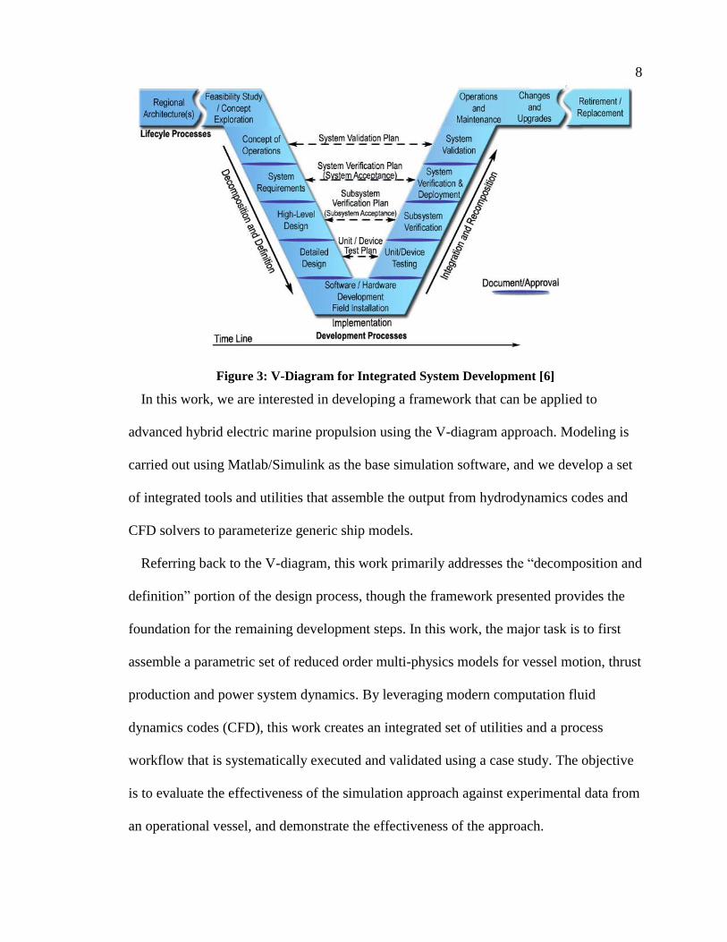
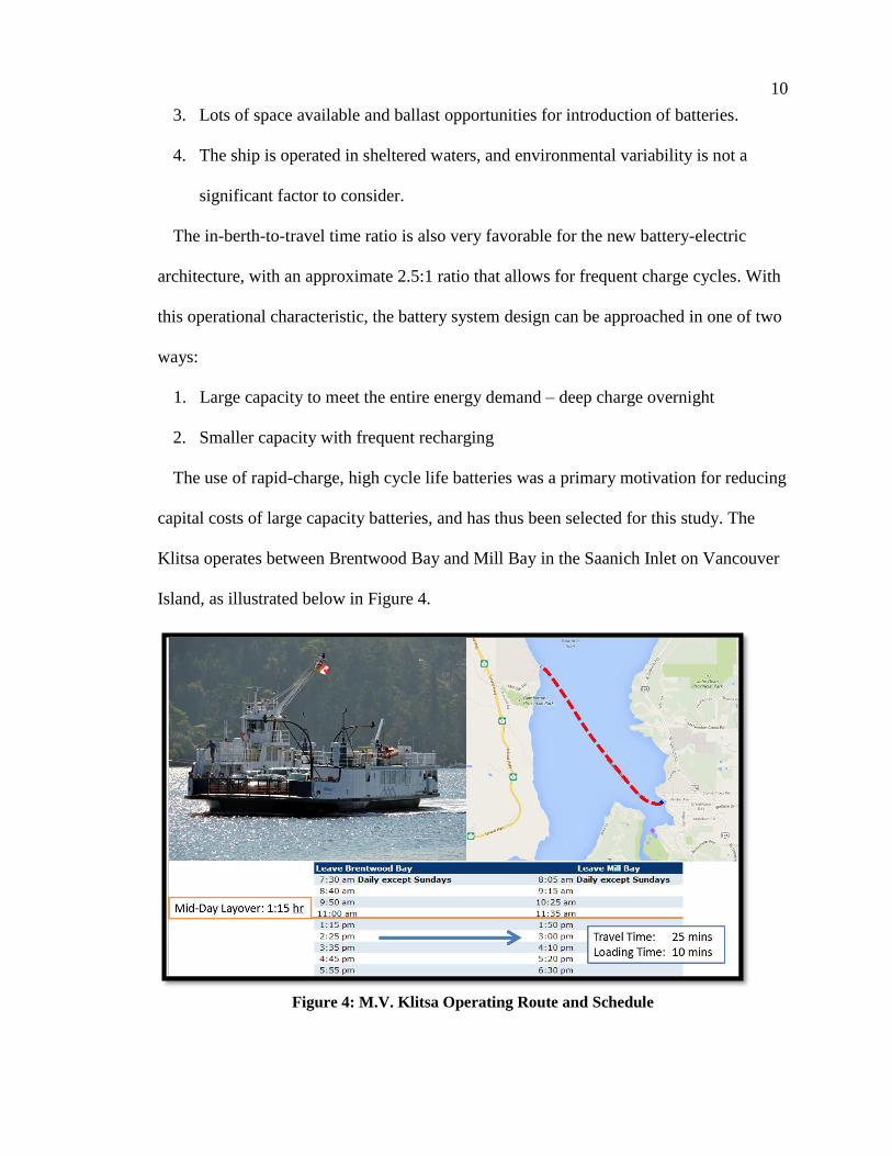
Klitsa operates between Brentwood Bay and Mill Bay in the Saanich Inlet on Vancouver

Island, as illustrated below in Figure 4.

Figure 4: M.V. Klitsa Operating Route and Schedule

11

The ship makes eighteen crossings per day, with eight in the morning, and ten in the

afternoon. The schedule also allows for a one hour mid-day layover where the ship is

tied-up in Brentwood Bay. A breakdown of the charging availability as defined by

current BC Ferries sailing schedule is provided below in Table 1.

Table 1: Charging Availability under Current Operating Schedule

Energy Storage Charge Type Charge Time

Availability (Hours)

Slow Charge Cycles Overnight Charging Time 12.5

Mid-Day Layover Time 1.15

Rapid Charge Cycles Loading/Unloading Charging Time 0.17

Number of Load/Unload Cycles 16

Total Rapid Charge Potential 2.67

The plant model of the Klitsa’s existing propeller system and hull is systematically

presented in Chapter 3, and 4 respectively. A comprehensive data acquisition study was

also conducted as part of this project to provide a means of validation for the models.

Details on the data acquisition experiment can be found in Appendix A.

The Klitsa is currently equipped with two 14L Series 60 Detroit Diesel engines, each

coupled to a well-mounted azimuthing thruster system located at opposite ends of the

ship. The azimuth angle is oriented using a PTO-based hydraulic system driven from the

main driveshaft. Electrical power is provided by one of two auxiliary 50kW marine diesel

generators. The main and auxiliary diesel engines provide the entire energy supply to the

vessel during operation. Upon completing its daily schedule, the ship is connected to

shore-power with all the engines and generators turned off.

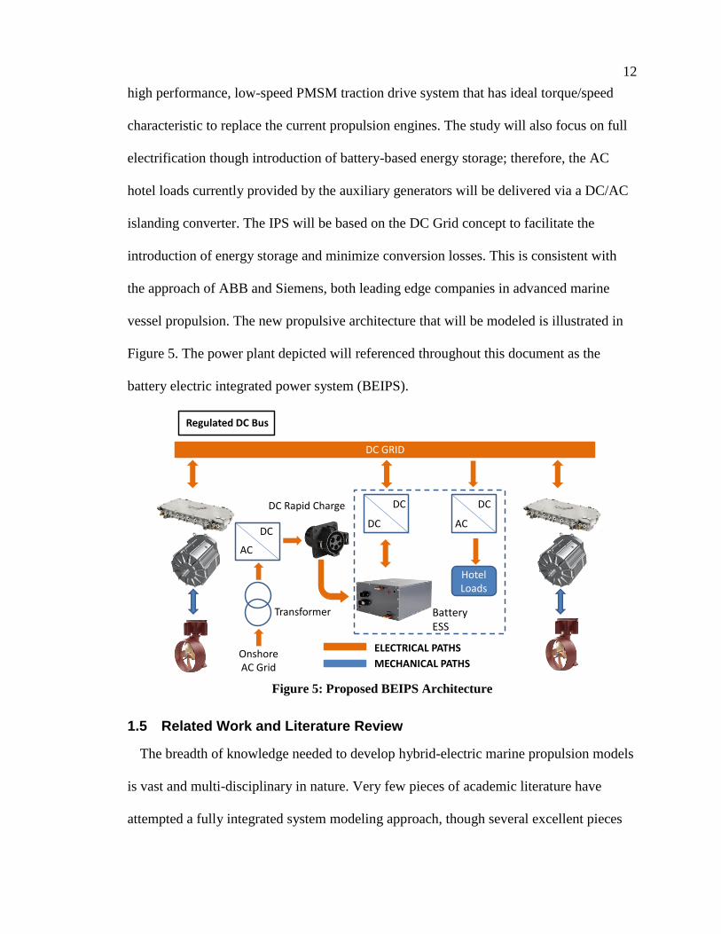
For the purposes of this study, it will be assumed that the main engines are to be

replaced with a commercially available electric drive system. The motor selected is a

12

high performance, low-speed PMSM traction drive system that has ideal torque/speed

characteristic to replace the current propulsion engines. The study will also focus on full

electrification though introduction of battery-based energy storage; therefore, the AC

hotel loads currently provided by the auxiliary generators will be delivered via a DC/AC

islanding converter. The IPS will be based on the DC Grid concept to facilitate the

introduction of energy storage and minimize conversion losses. This is consistent with

the approach of ABB and Siemens, both leading edge companies in advanced marine

vessel propulsion. The new propulsive architecture that will be modeled is illustrated in

Figure 5. The power plant depicted will referenced throughout this document as the

battery electric integrated power system (BEIPS).

Figure 5: Proposed BEIPS Architecture

1.5 Related Work and Literature Review

The breadth of knowledge needed to develop hybrid-electric marine propulsion models

is vast and multi-disciplinary in nature. Very few pieces of academic literature have

attempted a fully integrated system modeling approach, though several excellent pieces

DC GRID

DC

DC

MECHANICAL PATHS

ELECTRICAL PATHS

DC Rapid Charge

Regulated DC Bus

DC

AC

HotelLoads

AC

DC

OnshoreAC Grid

Transformer Battery ESS

13

of work have focused on modeling and simulation of the IPS. On the vessel side, a large

pool of literature can be found on predicting ship motion and motion control systems

which forms a solid foundation for creating parametric vessel models. Models describing

the mechanics and dynamics of thrust production for time-domain simulation provide the

background for describing the energy conversion between power system and ship

actuation. Finally, we can draw upon the extensive field of academic literature

surrounding hybrid-electric vehicles in the automotive sphere and extend this knowledge

to advanced marine propulsion. To summarize, the related research can be categorized as

follows:

a) Marine vessel integrated power system modeling

b) Hybrid-electric vehicle technology

c) Mechanics and dynamics of thrust production

d) Ship motion and control

A brief review of related literature for each of these categories is presented in the

following sections. Note that in this work, there is particular interest in developing a

battery electric vehicle concept with rapid charging infrastructure; therefore, the literature

pertaining to this architecture will be been emphasized.

1.5.1 Integrated Power System Modeling for Hybrid Marine Propulsion

With the trend towards further ship electrification, many bodies of work have focused

on modeling, simulation, and control of integrated marine power systems. The models

developed are typically used to study power system stability, reliability, fault recovery,

and advanced energy management. Much of this work has been developed for military

applications, though many recent studies have focused on commercial applications like

14

ocean service vessels. Comprehensive reviews of AES technology including

subcomponents and distribution systems are provided by Thongam et al. [7], McCoy and

Amy [8], and Tessarolo et al [9].

The most relevant literature related to this work is provided by a series of papers

published by Zahedi, which develop a system-level model of an AES including fuel cell

and batteries. First, Zahedi et al. [10] develop an average value model for an isolated bi-

directional DC/DC converter for system-level simulation. Second, Zahedi et al. [11]

develop a low voltage DC integrated power system model using an average value

modeling approach for converters based on a d-q reference coordinate transformation.

The authors illustrate the computational efficiency with this approach and its

effectiveness for system-level studies. In a third paper [12], the authors develop a control

framework for real-time energy management based on component efficiencies.

Some studies have attempted to couple the integrated power system simulation with the

hydrodynamics of thrust production. Prempraneerach et al. [13] develop an integrated

power system model for an AES with some propeller dynamics to simulate the effects of

extreme events on the IPS, such as pulsed weaponry and propeller emergence. Extreme

events are applied using a stochastic framework. Zahedi et al. [11] also incorporated

propeller dynamics and deployed the Simulink-based Marine Systems Simluator (MSS)

toolbox for the vessel model, though thrust production is simplified and details of the

ship model are not given. Apsley et al. [14] also develop reduced order average value

component models for the power system. Furthermore, the authors couple the propeller

load to the ship forward speed while accounting for wake fraction effects.

15

Many other pieces of work have conducted simulation studies for AES performance in

academic literature, for example, Ouroua et al [15], Weng et al. [16], or Jaster [17], each

with a slightly different focus. Though these studies do make an attempt to incorporate

the vessel and propeller dynamics to give a physical sense of the load, most studies

assume that power system loads that are either,

a) assumed to be at steady state,

b) assumed to encounter arbitrary dynamic changes, or,

c) are studied while the ship is executing a single maneuver.

A comprehensive reference from Hansen et al. [18] discusses the mathematical

modeling of individual system components, distribution systems, and thrust production to

generate a state space representation of diesel-electric marine propulsion systems.

Though the work referenced above provides an excellent starting point, very few studies

present validation against real operational data to confirm the approach. The only

exception is Ahmadi et al. [19] where small-scale bench testing was performed.

The work presented in this thesis is building towards development of real-time energy

management and advanced control systems for marine vessels. Several excellent pieces

of work have been developed in this area including Seenumani [20], Radan [21], Wei et

al. [22], and Zahedi et al. [12]. Though these works are not explicitly used in this work, it

will be seen that the underlying principle of system efficiency optimization will overlap

with much of the discussion presented moving forward.

1.5.2 Hybrid Electric Vehicle Technology

Hybrid-electric vehicles have received a large amount of research attention over the

past ten years, most of this work relating to energy management, optimal control, and

16

system design/optimization. Literature on the subject is indeed vast, but two

comprehensive references in Husain [23] and Emadi [24] provide an excellent overview

of the fundamentals of system/component modeling and HEV design process. Consumer

automobiles are by far the most studied application of HEV technology. By comparison,

consumer vehicles are relatively low-power when contrasted with marine vessels.

The case study of the Klitsa seeks to investigate a large-scale energy storage system

with rapid charging infrastructure that forms the basis of the BEIPS architecture. The

LTO battery chemistry has been selected for modeling as these batteries have already

been successfully demonstrated in commercial rapid-charge transit bus applications. In

the following sections, we focus on relevant literature to modeling the BEIPS

components.

1.5.2.1 Converter Modeling and Averaging Techniques for System-Level Studies

Adoption of energy storage in hybrid electric marine propulsion applications requires

the use of a DC/DC converter for interfacing with the DC distribution bus [2]. A full

bridge isolated bi-directional DC/DC converter topology for shipboard applications of

energy storage systems has been explored by Chung et al. [25] and Zahedi and Norum

[26]. The converter integrates an active clamp on the current-fed side which is discussed

in Yakushev et al. [27]. A similar unidirectional converter using zero voltage switching

(ZVS) is presented in Prasanna and Rathore [28].

The objective is to develop a signal averaged model that is computationally efficient

and suitable for system-level studies. A comprehensive review of averaging techniques is

provided by Chiniforoosh et al. [29], and general discussion can be found in Erikson [30]

and Rashid [31]. Zahedi et al. [26] explore the different averaging methods for a full

17

bridge bi-directional converter to evaluate the large and small signal performance versus

computational efficiency. Further discussion on application of DC/DC converters to

hybrid vehicle design can be found in Emadi [24] and Husain [23].

1.5.2.2 Permanent Magnet Synchronous Machine Modeling and Control

The electric propulsion system to be modeled in this work will be based off a

commercially available PMSM drive package. A detailed derivation of the simulation

model for a PMSM and voltage source inverter (VSI) drive systems is presented in

Krause [32], and Krishnan [33]. Power loss models based on efficiency lookup tables, as

well as simulation models are discussed in Husain [23] in the context of hybrid electric

vehicle performance analysis. A discussion of steady state motor and inverter losses for

PMSM-based drives systems using MTPA control are discussed by Chao, Chen and

Diwoky [34] for predicting efficiency maps for traction drive system. This study includes

both iron and copper losses for the motor, as well as semiconductor losses in the inverter.

Sources of losses and loss minimization techniques for PMSMs are also discussed in

Hassan and Wang [35].

The implementation of MTPA control strategies is discussed in Ahmed [36]. Zheng

and Hongmei [37] discuss MTPA control and the effects of saturation and cross-

coupling. The authors also discuss offline optimization techniques for building MTPA

reference generators.

Two-level inverter bridges and modulations strategies are discussed in detail in Krause

[32]. In this work, space vector pulsed width modulation (SVPWM) will be modeled to

be consistent with the commercial drive system. Krause [32] presents the switching

algorithm which will be implemented for performance comparison of the AVM model

18

with a detailed switching model. Chao, Mohr and Diwoky [34] use the semiconductor

loss model for SVPWM presented in Bierhoff and Fuchs [38] to generate loss predictions

for the inverter in steady state. Trzynadlowski and Legowski [39] discuss losses

associated with vector PWM methods while Zhou and Wang [40] perform a comparative

analysis between SVPWM and other three-phase carrier based PWM strategies.

1.5.2.3 Battery System Modeling with Thermal Effects

Battery models have been integrated into many of the AES and/or IPS modeling

studies previously mentioned. A comprehensive overview of lithium battery systems and

their electro-chemical governing equations is provided by Rahn [41]. More simplified

equivalent circuit based models are discussed in Chen and Rincon-Mora [42], and the

authors present a dual polarization model that has been applied to the LTO chemistry in

Cleary et al. [43], Stroe et al. [44], Erdinc [45] to name few. The process of fitting

equivalent circuit parameters to experimental data and constructing an equivalent circuit

model is described Huria et al. [46]. Reduced order electrochemical models can also

provide a good platform for system-level studies, though they require more intimate

knowledge of the cell parameters. The single particle model for a lithium battery is

discussed by Ahmed in [47] and [48], which illustrates the models effectiveness in

adapting to degradation.

The work conducted by Cleary et al. [43] involved performance testing of a 9.2kWh

battery pack comprised of LTO modules, and the experimental data was fit to a dual

polarization type equivalent circuit approximation. The authors published a near-

complete set of data for the equivalent circuit parameters that is used to create the large-

scale pack model in this work. Further work on experimental testing of LTO modules is

19

provided by Lin et al. [49], while the LTO’s experimental performance in fast-charging

is discussed in Burke et al. [50].

The equivalent circuit model can also be coupled to a thermal model as is done in

Erdinc et al. [45], Huria [46], and Clearly et al. [43]. This will constitute future work, and

a wealth of additional references can be found in this area.

In this work, the focus is on development of a large-scale dual polarization equivalent

circuit model that will be parameterized using the data offered by Cleary et al. [43].

When experimental data can be generated in-house, this model will later be replaced with

the reduced order electrochemical model to provide a better framework for capturing

degradation.

1.5.3 Thruster Dynamics Modeling

The field of literature relating to propeller performance is extensive. General references

on the topic can be found in Carlton [51], Kerwin [52], and Breslin and Andersen [53],

each providing a wide discussion on traditional topics relating to propeller geometry,

design, performance, and analysis. Kerwin [52], along with subsequent papers from Epps

[54] and Epps and Kimball [55] provide a comprehensive review of vortex-lattice lifting

line (VLL) methods for analytical analysis and design of propellers in first quadrant

operation. Though not explicitly used in this work, this computationally efficient

propeller analysis code provides future opportunities for global system-level optimization

within the MIL platform.

Modeling the dynamics of thrust production was initially studied for ROV/AUV

applications, largely within the context of model based control synthesis. Initial work by

Yoerger et al. [56] and Healey et al. [57] established a thrust dynamics model based on

20

momentum theory which was expanded upon by Blanke et al. [58], Bachmayer et al. [59]

to include different mapping techniques for relating thrust and torque functions to state

variables. Blanke et al. [58] provided a method of relating open water propeller

coefficients to the dynamics model, but used linear approximations for open water

curves. This work only investigated positive advance ratios (first quadrant) under normal

incident flow conditions. Kim and Chung [60] extended this work to a quadratic

framework over two quadrants in order to better represent typical open water curves;

however, the dynamics of thrust production were ignored. The authors also studied the

performance of a thruster in first and pseudo-second quadrant operation, and at various

incident flow angles, providing insight into the thrust and torque curves for the rotatable

azimuthing propellers. Note, the term pseudo-second quadrant has been coined in this

term to differentiate between propeller reversing direction, and a 180° rotation of an

azimuthing propeller. This will be explained further in Chapter 3.

1.5.4 Vessel Dynamics Modeling – Maneuvering and Seakeeping

The study of vessel motion in response to waves while traveling on a fixed course is

termed seakeeping analysis. Seakeeping analysis can be performed in either the

frequency or the time domain. Cummins [61] developed a mathematical relationship

relating the dissipative radiation force that results from ship motion to the frequency

dependent added mass and damping coefficients produced from inviscid theory. Faltinsen

[62] and Fossen [63] provide comprehensive references that discuss the forces and

response of vessels when subject to waves. McTaggart [64], [65] provides an excellent

discussion of sea loads and the motion response of ships in the supporting documentation

for ShipMo3D. Seakeeping modeling is conducted using hydrodynamic coefficients

21

computed from 2D strip-theory or 3D potential flow solvers. ShipMo3D is a 3D potential

flow solver used in this work. The computation of hydrodynamic coefficients is discussed

in Newman [66], McTaggart [67], and an example of a boundary element algorithm is

given in Bertram [68].

Maneuvering models, in contrast, are concerned with the ship’s motion and trajectory

when executing a specific maneuver. Maneuvering models have not achieved the same

level of accuracy as seakeeping methods [68], largely due to the complex fluid

interactions that arise during the maneuver. The vessel experiences large displacements in

six degrees of freedom (DOF) relative to its nominal cruise state which is difficult to

represent with reduced order models. Abkowitz [69] presented a non-linear maneuvering

model that has been extensively used in literature but requires coefficients from

experimental planar motion mechanism (PMM) tests. In more recent years, researchers

have been looking to generate these coefficients using uRANS CFD as is done in

Simonsen et al. [70].

Fossen [63] discusses various maneuvering models including Ross el al. [71], where

the authors develop a more physical model derived from low aspect ratio wing theory.

Fossen [63] and McTaggart [65], [72] discuss a unified maneuvering/seakeeping

approach for time-domain simulation that can be used for motion control system

development. This unified approach, which blends seakeeping and maneuvering models

has some limitations which are discussed in Chapter 4. Lastly, McTaggart [73], Ikeda et

al. [74], [75] and Kato [76], [77] discuss the forces on appendages which has direct

relevance to the case study of the Klitsa.

22

1.6 Thesis Roadmap

This thesis develops an integrated modeling framework and parameterization

workflow, complete with tools and utilities, to enable model based development and

simulation of advanced marine propulsion systems. This framework compiles the related

research discussed in the previous section to create a computationally efficient system-

level model that includes integrated power system, vessel motion, and thrust production

dynamics.

The first objective is to develop a reduced order, multi-physics simulation framework

that represents the M.V. Klitsa. The parameterization procedure and model structure is

designed to be generic and applicable to any ship. The vessel dynamics model required

by marine vessels is considerably more involved than that of a consumer automobile. The

complex fluid phenomena governing the ship motion requires the use of hydrodynamic

codes, uRANS CFD, and other types of hydrodynamic analyses to generate the necessary

parametric data. The same is true for azimuthing propeller system. By deploying CFD

through a series of well-defined experiments, parametric data can be generated to

represent the full spectrum of operating conditions for the ship’s hull and propeller

models. This objective is addressed in Chapters 2, 3 and 4.

The second objective is to explore the use of battery-electric technology as part of the

case study of the M.V. Klitsa. With the BEIPS concept having struck the interest of BCF,

this thesis presents a preliminary design and parametric model of the BEIPS architecture

to study its performance on the Brentwood Bay – Mill Bay crossing. This objective

drives the work in Chapter 5.

The final objective is to compare the system-level model’s performance against the

ship’s real-world operating data to assess the effectiveness of the approach in predicting

23

propulsive loads, and energy consumption. This objective is met by first defining a

standard set of load profiles based on observation of the data collected, then comparing

this data with the model’s output when subjected to the same driver inputs. This work is

presented in Chapters 6, and 7.

The multi-disciplinary scope required to assemble such a system-level model, which

includes proper treatment of governing hydrodynamics coupled with hybrid electric

power systems, is substantial; therefore, Chapter 2 compiles a review of relevant theory

and fundamentals that will make up the overall model including,

1. Dynamical thrust production in multiple quadrants for development of an

azimuthing propeller model that interfaces with powertrain mechanical loads

2. Unified maneuvering/seakeeping theory used for representing the vessel dynamics

3. Electric power system modeling with an emphasis on the BEIPS architecture

Once the necessary theory has been developed, Chapter 2 concludes with an overview

of the model integration strategy, parameterization methodology, and general workflow.

This approach is then systematically executed over the remaining chapters.

Chapter 3 develops a dynamical model of the existing well-mounted azimuthing

thrusters for pseudo four-quadrant operation. This will enable a direct comparison of the

model with real data collected from the ship. The model is developed using results

produced by RANS CFD for on/off design conditions.

Chapter 4 develops a dynamical vessel model using a unified seakeeping/maneuvering

approach with surge resistance parameterized from CFD studies. Hydrodynamic

coefficients for the Klitsa’s hull are generated by ShipMo3D, and interfacing utilities are

24

developed to make use of pre-defined blocks offered by the Marine Systems Simulator

(MSS) toolbox for Simulink [78].

Chapter 5 develops a system-level BEIPS model aimed at computational efficiency,

employing a combination of average value and power loss modeling. This chapter

provides a preliminary system design based on commercially available components.

Validation of the overall system-level model is performed by comparative analysis

using data collected from a comprehensive data acquisition experiment conducted as part

of this work. This experiment developed a custom CAN-based data collection network

that interfaced with onboard ship systems and standalone instrumentation. Details of the

experiment have been excluded in the body of this document, but the key results are

presented in Chapter 6. Here, three representative load cycles are developed to reflect the

normal operational variability of the ship while in service.

Chapter 7 assembles all of the system components into a single simulation, and uses

the load profiles of the data acquisition study to compare the powertrain load predictions

produced by the model. Lastly, Chapter 8 provides a set of conclusions and highlights

areas for future improvement.

1.7 Research Contributions

Though many propulsion modeling and simulation studies have been performed in

literature, these modeling studies are often subjected to arbitrary or short-term load

conditions aimed at illustrating the model’s response to a specific event. In this work, the

objective is slightly different in that we seek to develop an integrated system model that

is capable of predicting energy demands of the ship over a mission cycle, such that

different the performance of hybridized architectures can be compared. This functionality

25

allows for both control and system level optimization of the propulsion system in the

design stage. To the author’s knowledge, no other work has sought to create a modeling

tool aimed at delivering this functionality.

This thesis provides the framework and methodology for high-level architectural

analysis, mirroring the functionality offered by software such as Autonomie or PSAT

used in the automotive industry. This approach allows for performance modeling using

metrics of fuel consumption and system-level conversion efficiency, while also providing

a foundation for Software-in-the-Loop and Hardware-in-the-Loop integrated

development for IPS and motion control systems. Unlike most other studies, the

modeling development process is validated using real-world data recorded from the

operational ship.

By illustrating the process through a case study, this work has concurrently sought to

assess the technological feasibility of a BEIPS propulsion architecture using rapid-charge

technology for BCF’s Brentwood Bay - Mill Bay crossing. This unique architecture is

similar to that of the Ampere, though with a more demanding crossing schedule that

resembles that of a transit bus. Summarizing, this thesis provides the following

contributions:

1. Develops and publishes real-life operational drivecycles that can be used for further

propulsion optimization studies.

2. Develops and validates an integrated modeling framework that allows for high

level system propulsion analysis through simulation, specifically focusing on

energy consumption, system efficiency, and emission reduction.

26

3. Develops a preliminary BEIPS power system design and system model based on

commercially available components for assessing technical feasibility of battery

electric ship with rapid-charge.

4. Creates software utilities for integration of the MSS toolbox with ShipMo3D and

ProteusDS output files.

5. Develops an average value model for an electric machine with dynamic losses for

predicting electric drive efficiency. Model is compared with actual published data

from manufacturer.

6. Develops a realistic large-scale LTO battery dynamic model based on pack-level

experimental data.

7. Provides a parameterized ship model for the M.V. Klitsa that can be used for

further architectural studies, alternate route simulations, auto-pilot control system

development, or Software-in-the-Loop integrated controller development.

27

Chapter 2 Ship Propulsion Modeling and Dynamics

Chapter 1 established the motivation for developing an integrated time-domain

modeling platform for simulation of hybrid electric marine propulsion. With this type of

analysis tool, the designer can simulate the overall performance of the ship under

different operating conditions so to optimize the propulsion system architecture and

power delivery. This is a significant departure from the traditional design approach used

in naval architecture, which is largely a quasi-static design process optimized about

particular operating points.

The traditional approach to ship propulsion design and its decomposition is an

excellent starting point for the discussion. Thus, this chapter begins with a brief

introduction on the subject matter to draw relevant information from the classical

literature. This includes a brief overview of propulsive coefficients, hull-propeller

interaction quantification, and propulsive efficiencies. The propulsion discussion

provides a logical segue into propeller modeling theory, which forms the critical interface

between the IPS and the vessel motion.

Next, the governing equations and simulation models for components making up the

BEIPS architecture are presented individually. This is followed by a summary of unified

seakeeping/maneuvering theory that will be used to develop the vessel motion dynamics

model. Finally, this chapter concludes by presenting the overall model architecture and

proposed parameterization methodology. This includes a strategy for systematic use of

computational fluid dynamics and integration of hydrodynamic solvers.

28

2.1 Ship Propulsion – An Introduction

The design of a ship’s propulsion system is a complex and often multiple objective

optimization problem. The ship must be capable of safe operation under all anticipated

conditions, and must meet all of the performance specifications issued in the design

contract. At the fundamental level, the typical propulsion system consists of three

components:

1. Prime mover – Responsible for converting chemical energy to mechanical energy

2. Transmission system – Responsible for transporting energy from prime mover to

propulsor

3. Propulsor – Converts mechanical rotational energy into a thrust force [4].

Traditionally, the prime mover is a diesel engine or a gas turbine. The transmission

system can be either electrical, or mechanical depending on the architecture. In recent

years, the AES has been increasing in popularity. In this electrified configuration, the

ship’s hotel and propulsive demands are drawn from a common electrical supply.

The propulsion system produces a thrust force on the vessel which needs to overcome

the hull resistance. In the absence of the propeller, the hull’s resistance is comprised of

three components:

Frictional or viscous resistance, defined as the resistive force produced by

tangential forces in the flow as a consequence of the boundary layer.

Form or pressure resistance, defined as the resistive force from the pressure

imbalance acting on the hull.

Wave resistance, defined as the drag force associated with imparting energy into

the wave system produced by the ship’s motion.

29

A more thorough treatment of resistance is provided in an upcoming section as part of

the vessel dynamics modeling. It is largely recognized that a good approximation for ship

resistance with respect to the vessel’s forward speed is given by,

𝐹𝑅 = 𝑐1𝑉𝑠2 ( 2-1 )

Here, 𝐹𝑅 represents the total hull resistance, 𝑉𝑠 is the ship forward speed, and 𝑐1

represents the proportionality constant. The effective power required to tow the hull is

given by,

𝑃𝐸 = 𝐹𝑅𝑉𝑠 ( 2-2 )

The effective power delivered by the propeller is characterized by the thrust force (T)

multiplied by the advance speed of the propeller (𝑉𝑎).

𝑃𝑇 = 𝑇𝑉𝑎 ( 2-3 )

The thrust produced by the propeller exceeds that of the hull’s effective towing

resistance. The process of accelerating flow along the hull by means of the propeller

creates an increased pressure imbalance, adding to the resistive force. This effect is

typically characterized using a thrust deduction factor defined as,

𝑡 =𝑇 − 𝐹𝑅𝑇

( 2-4 )

This relationship can be augmented in the event of 𝑘𝑝 propellers on the vessel as

follows:

𝑡 =𝑘𝑝𝑇 − 𝐹𝑅

𝑘𝑝𝑇 or, 𝑅 = (1 − 𝑡)𝑘𝑝𝑇 ( 2-5 )

30

The thrust deduction factor is typically determined experimentally with scale-model

tow tank testing, though self-propelled CFD studies have been show to produce good

approximations.

The advance velocity of the propeller differs from the forward speed of the ship. As the

ship moves through the water, a boundary layer develops around the hull effectively

slowing down the inflow velocity seen by the propeller(s) at the aft of the ship. The wake

fraction w provides an empirical term to quantify this interaction and is defined by,

𝑤 =𝑉𝑠 − 𝑉𝑎𝑉𝑠

or, 𝑉𝑎 = (1 − 𝑤)𝑉𝑠 ( 2-6 )

At the stern of the ship, the boundary layer has typically grown sufficiently thick that the

propeller operates fully in this viscous region [4]. The corrected advanced velocity 𝑉𝑎 is

a somewhat fictitious term that is determined by analyzing the flow field at the

propeller’s location in relative to the hull. In actuality, the propeller is accelerating the

flow and the velocity is significantly higher as will be discussed later. The total hull

efficiency, as a measure of power input to the propeller versus effective power output that

produces motion is given by,

𝜂𝐻 =𝑃𝐸𝑘𝑝𝑃𝑇

=(𝐹𝑅𝑉𝑠)

𝑘𝑝(𝑇𝑉𝑎)=1 − 𝑡

1 − 𝑤 ( 2-7 )

2.1.1 Propeller Efficiency

The energy supplied to the propeller is provided by rotational mechanical energy. The

performance characteristics of propellers are typically given for open water conditions, in

absence of the hull. The open water propeller efficiency, 𝜂𝑂, is determined by the ratio of

31

effective thrust power produced versus the rotational mechanical power delivered to the

propeller with torque Q, and angular speed ωp.

𝜂𝑂 =𝑃𝑇𝑃𝑂=𝑇 ∙ 𝑉𝑎𝑄 ∙ 𝜔𝑝

=𝑇 ∙ 𝑉𝑎

2𝜋(𝑄 ∙ 𝑛𝑝) ( 2-8 )

Typical values for open water efficiency range from 0.3 to 0.7 depending on class of

vessel [4]. When operating behind a ship’s hull, the actual power delivered to the

propeller is slightly different than its open-water value. This discrepancy is accounted for

using the relative rotative efficiency defined by:

𝜂𝑅 =𝑃𝑂𝑃𝑃=𝑄 ∙ 𝜔𝑝

𝑀𝑃 ∙ 𝜔𝑝=2𝜋(𝑄𝑂 ∙ 𝑛𝑝)

2𝜋(𝑀𝑃 ∙ 𝑛𝑝)=𝑄

𝑀𝑃 ( 2-9 )

Note 𝑀𝑃 represents the mechanical input torque to the propeller while operating behind

the hull, where 𝑄 represents the torque observed in open water conditions at the same

advance ratio. This efficiency is typically close to unity, often ranging from 0.98 to 1.02.

It encompasses the losses from non-uniform inflow conditions at the propeller [4].

2.1.2 Mechanical Transmission Chain

Traditional diesel, full-electric, and hybrid propulsion architectures have different

losses associated with mechanical power transmission. Mechanical transmission losses

occur in gearboxes, driveshafts, bearings, stuffing boxes, seals, and driveline couplings.

When medium speed engines and/or electric speed drive systems are specified, a gearbox

is required to reduce shaft speed, and increase output torque to drive the propeller as

shown in Figure 6. The transmissive efficiency, which describes the low-speed

mechanical power transmission linking the propeller to the gearboxes output shaft is

expressed as,

32

𝜂𝑠 =𝑃𝑃𝑃𝑆=𝑀𝑃𝑀𝑆

( 2-10 )

𝑃𝑆 = 𝑀𝑆 ∙ 𝜔𝑝 = 2𝜋 ∙ 𝑀𝑆 ∙ 𝑛𝑝 ( 2-11 )

Here, MS is the torque output of the gearbox and MP is the torque delivered to the

propeller. The subscript “S” denotes quantities at the output of the gearbox. The shaft loss

efficiency typically lies between 0.5% and 1% of the nominal power and accounts for

frictional losses in the stern tube and shaft bearings [4].

Figure 6: Illustration of Parallel Drive Gearbox (Top) and Right Angle Gearbox (Bottom)

Configurations

The power delivered by the engine is described by the engine brake power, PB, which

is expressed by the basic mechanical rotational power relation,

𝑃𝐵 = 𝑀𝐵 ∙ 𝜔𝑒 = 2𝜋 ∙ 𝑀𝐵 ∙ 𝑛𝑒 ( 2-12 )

33

Denoting the gear reduction with the variable nGB, the efficiency through the gearbox is

expressed as,

𝜂𝐺𝐵 =𝑃𝑆

𝑘𝑒 ∙ 𝑃𝐵=

𝑀𝑆 ∙ 𝑛𝑝

𝑘𝑒 ∙ 𝑀𝐵 ∙ 𝑛𝑒=

𝑀𝑠𝑘𝑒 ∙ 𝑀𝐵

∙1

𝑛𝐺𝐵 ( 2-13 )

where,

𝑛𝐺𝐵 =𝑛𝑒𝑛𝑝

( 2-14 )

Gearbox losses are typically 1-2% in a single-stage parallel shaft reduction, typically

used with medium speed diesel engines. For multi-input parallel gearboxes and more

complex multiple reduction systems, the losses are higher, generally 3-5% [4]. Right

angle drive gearboxes, such as those used in azimuthing propellers, can have losses

greater than 5%.

The total mechanical transmission efficiency is the product of mechanical drivetrain

efficiencies,

𝜂𝑇𝑅𝑀 =𝑃𝑃

𝑘𝑒 ∙ 𝑃𝐵=

𝑀𝑃𝑘𝑒 ∙ 𝑀𝐵

∙1

𝑛𝐺𝐵=𝑀𝑃𝑀𝑆

∙𝑀𝑆

𝑘𝑒 ∙ 𝑀𝐵∙1

𝑛𝐺𝐵= 𝜂𝑆𝜂𝐺𝐵 ( 2-15 )

The total propulsive efficiency is summarized by Figure 7. It’s important to note that

the propulsive efficiency will vary depending on the operating speed of the vessel. The

previous discussion applies to efficiencies taken at design speed, when in reality the

losses are a function of the vessel’s operating point. For example, mechanical rotational

losses are well described by damping function that includes of Coulomb, linear, and non-

linear damping effects, see for example Pivano [79]. However, the preceding discussion

helps in understanding sources of loss to be considered in the dynamic simulation

models.

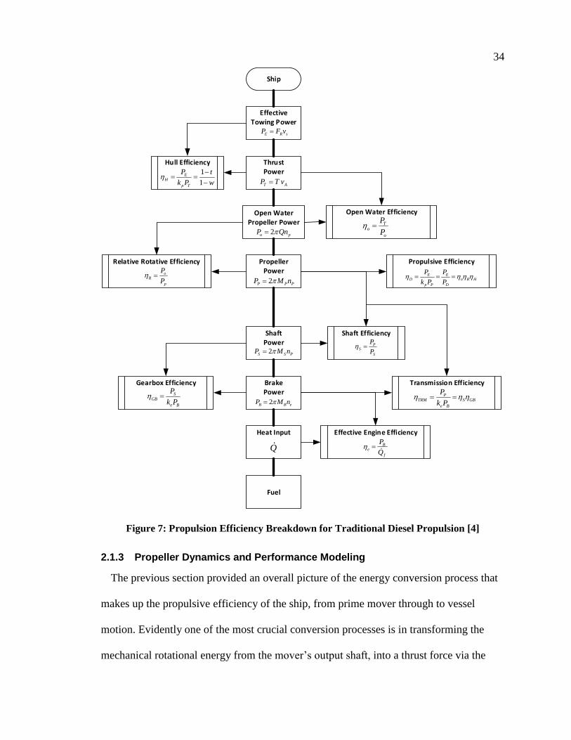
34

Transmission Efficiency

Propulsive Efficiency

Open Water Propeller Power

Shaft Efficiency

Relative Rotative Efficiency

Ship

Effective Towing Power

Thrust Power

Propeller Power

Shaft Power

Brake Power

Heat Input

Fuel

Hull Efficiency

1

1

EH

p T

P t

k P w

E R sP F v

T AP T v

Open Water Efficiency

To

o

P

P

2o pP Qn

oR

p

P

P

2P P PP M nE E

D o R H

p P D

P P

k P P

PS

S

P

P

2S S PP M n

PTRM S GB

e B

P

k P

Gearbox Efficiency

SGB

e B

P

k P

2B B eP M n

Q

Effective Engine Efficiency

Be

f

P

Q

Figure 7: Propulsion Efficiency Breakdown for Traditional Diesel Propulsion [4]

2.1.3 Propeller Dynamics and Performance Modeling

The previous section provided an overall picture of the energy conversion process that

makes up the propulsive efficiency of the ship, from prime mover through to vessel

motion. Evidently one of the most crucial conversion processes is in transforming the

mechanical rotational energy from the mover’s output shaft, into a thrust force via the

35

propeller. The presence of the hull influences the inflow profile and operating conditions

of the propeller, and other fluid-structure interactions can significantly impact on its

performance. Literature on the subject is vast with the most comprehensive references

presented by Carlton [51], Kerwin [52], and Breslin and Anderson [53].

In this work, the primary objective is to develop a model that can accurately predict

powertrain loads from a freely maneuvering ship. During maneuvering, the ship’s

propellers will regularly encounter off-design conditions that can drastically change the

load on the IPS. The Navier-Stokes equation defines the complex fluid mechanics

governing thrust production, but is too computationally intensive to utilize in a system-

level model; therefore, the standard propulsive coefficients provide a good starting point

for reduced order model development.

The approach here draws on literature relating to model-based vessel motion control

systems for surface vessels and AUVs/ROVs. Not only does the development of accurate

propeller models allow for higher precision position and motion control, but it also

enables opportunities for advanced IPS energy management and control.

Open-water propeller performance for both thrust and torque is typically plotted as

non-dimensionalized coefficients KT and KQ versus the non-dimensionalized advance

ratio J, where,

Advance Ratio 𝐽 = 𝑉𝑎𝑛𝐷

( 2-16 ) 𝑉𝑎: Advance Speed (m/s)

𝑛: Propeller Speed (rev/s)

𝐷: Propeller Diameter (m)

𝑇: Thrust (N)

𝑄: Torque (Nm)

Thrust

Coefficient 𝐾𝑇 =

𝑇

𝜌𝑛2𝐷4 ( 2-17 )

Torque

Coefficient 𝐾𝑄 =

𝑄

𝜌𝑛2𝐷5 ( 2-18 )

36

These coefficients represent steady state, first quadrant operation where the propeller is

providing thrust to propel the vessel forward. When non-incident flow is encountered, or

the propeller is not deeply submerged, the propeller performance characteristics will be

different. Non-incident flow over the propeller will be encountered regularly during ship

maneuvers, as well as in the presence ocean currents and waves. One problem with these

standard definitions is that a discontinuity results when the propeller is at zero speed.

This is problematic during dynamic simulation if the propeller stops, or reverses

direction. Furthermore, these definitions are restricted to the first quadrant, and are don’t

extend conveniently into multiple quadrant operation. The quadrant of operation is

traditionally defined by the rotational direction of the propeller and the direction of ship

travel as described in Figure 8.

Figure 8: Traditional Definition of Propeller Quadrants

However, this definition needs to be expanded when referencing azimuthing propeller

system because 2nd and 4th quadrant operation are achieved by reorienting the propeller

by 180°. With this rotative functionality, another dimension can be added to Figure 8 to

describe all possible quadrants of operation as seen in Figure 9.

Ship Velocity

Propeller Angular Velocity

III

IVIII

β

37

Figure 9: Expansion of 4-Quadrant Definition to Represent Azimuthing Propellers

An alternate formulation of the advance ratio that eliminates the discontinuity at zero

speed is given by,

𝛽 = 𝑎𝑡𝑎𝑛2 (𝑉𝑎

0.7𝜋𝑛𝐷) ( 2-19 )

The parameter 𝛽 represents an angle that describes the quadrant of operation where,

0 ≤ 𝛽 ≤ 90° First Quadrant

90 < 𝛽 ≤ 180° Second Quadrant

180 < 𝛽 ≤ 270° Third Quadrant

270 ≤ 𝛽 < 360° Fourth Quadrant

This definition is convenient for handling off-design propeller conditions. Standard

non-dimensionalized propeller coefficients are limited in that they only represent steady

state operating condition; therefore, a dynamic framework should be formulated to better

accommodate time-domain simulation. Models for dynamic thrust production have been

proposed by Yoerger et al. [56], Healey et al. [57], Bachmayer et al. [59], Blanke et al.

Ship Velocity

III

IVIII

Aligned Azimuth Propeller

Reversed Azimuth Propeller

Propeller Angular Velocity

Ship Velocity

I

II’III

Aligned Azimuth Propeller

Reversed Azimuth Propeller

IV’ Propeller Angular Velocity

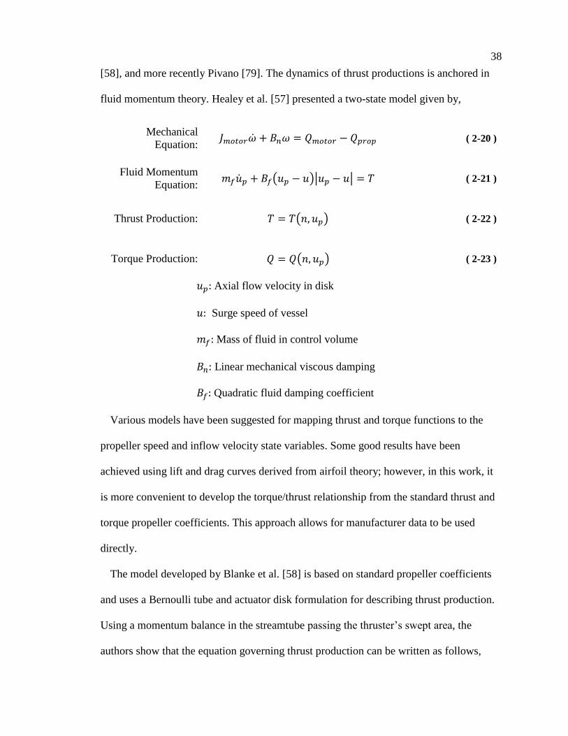
38

[58], and more recently Pivano [79]. The dynamics of thrust productions is anchored in

fluid momentum theory. Healey et al. [57] presented a two-state model given by,

Mechanical

Equation: 𝐽𝑚𝑜𝑡𝑜𝑟 + 𝐵𝑛𝜔 = 𝑄𝑚𝑜𝑡𝑜𝑟 − 𝑄𝑝𝑟𝑜𝑝 ( 2-20 )

Fluid Momentum

Equation: 𝑚𝑓𝑝 + 𝐵𝑓(𝑢𝑝 − 𝑢)|𝑢𝑝 − 𝑢| = 𝑇 ( 2-21 )

Thrust Production: 𝑇 = 𝑇(𝑛, 𝑢𝑝) ( 2-22 )

Torque Production: 𝑄 = 𝑄(𝑛, 𝑢𝑝) ( 2-23 )

𝑢𝑝: Axial flow velocity in disk

𝑢: Surge speed of vessel

𝑚𝑓: Mass of fluid in control volume

𝐵𝑛: Linear mechanical viscous damping

𝐵𝑓: Quadratic fluid damping coefficient

Various models have been suggested for mapping thrust and torque functions to the

propeller speed and inflow velocity state variables. Some good results have been

achieved using lift and drag curves derived from airfoil theory; however, in this work, it

is more convenient to develop the torque/thrust relationship from the standard thrust and

torque propeller coefficients. This approach allows for manufacturer data to be used

directly.

The model developed by Blanke et al. [58] is based on standard propeller coefficients

and uses a Bernoulli tube and actuator disk formulation for describing thrust production.

Using a momentum balance in the streamtube passing the thruster’s swept area, the

authors show that the equation governing thrust production can be written as follows,

39

𝑚𝑓𝑝 + 2𝜌𝐴𝑝|𝑢𝑝|(𝑢𝑝 − 𝑢𝑎) = 𝑇 ( 2-24 )

Note, Ap represents the propeller disk area. Using published open water performance

curves, the authors use a linear approximation to propeller curves described by the

following relationships,

𝐾𝑇 = 𝛼0 + 𝛼1 𝐽 =𝑇

𝜌𝑛2𝐷4 ( 2-25 ) ⇒

𝑇 = 𝛼0𝜌𝑛2𝐷4 + 𝛼1 𝜌𝑛

2𝐷4 (𝑢𝑎𝑛𝐷)

= 𝑇|𝑛|𝑛𝑛2 + 𝑇|𝑛|𝑣𝑛𝑢𝑎

( 2-26 )

𝐾𝑄 = 𝛾0 + 𝛾1 𝐽 =𝑄

𝜌𝑛2𝐷5 ( 2-27 ) ⇒

𝑄 = 𝛾0𝜌𝑛2𝐷5 + 𝛾1 𝜌𝑛

2𝐷5 (𝑢𝑎𝑛𝐷)

= 𝑄|𝑛|𝑛𝑛2 + 𝑄|𝑛|𝑣𝑛𝑢𝑎

( 2-28 )

where,

𝑇|𝑛|𝑛 = 𝛼0𝜌𝐷4 ( 2-29 ) 𝑄|𝑛|𝑛 = 𝛾0𝜌𝐷

5 ( 2-30 )

𝑇|𝑛|𝑣 = 𝛼1 𝜌𝐷3 ( 2-31 ) 𝑄|𝑛|𝑣 = 𝛾1 𝜌𝐷

4 ( 2-32 )

Here the coefficients 𝛼𝑖 and 𝛾𝑖 are fitted parameters. It is important to distinguish

between velocity parameters in these equations. The advance velocity 𝑉𝑎 in the original

definition needs to be re-evaluated within this dynamic framework. The ship’s forward

speed in surge is defined by the local frame velocity u. The ambient inflow conditions at

the inlet of the Bernoulli tube is corrected using the wake fraction to account for the

presence of the hull. The freestream velocity used to define propulsive coefficients

represents the inflow velocity to the streamtube. The actual velocity through the propeller

disk is higher as result of the flow acceleration, and this parameter is denoted by 𝑢𝑝. The

inlet to the streamtube, denoted by 𝑢𝑎, is synonymous with advance velocity computed

with the relationship,

40

𝑢𝑎 = (1 − 𝑤) ∙ 𝑢 ( 2-33 )

Blanke et al. [58] provide a derivation of the forces acting on a propeller blade to

generate an expression that relates flow velocity at the propeller to inflow condition,

𝑎 =𝑢𝑝

𝑢𝑎 ( 2-34 )

Using this definition, each governing equations can be expressed as a function of the

inflow velocity at the propeller. Blanke et al. [58] define the terms,

𝑇|𝑛|𝑣𝑜 = (

1

1 + 𝑎)𝑇|𝑛|𝑣 ( 2-35 ) 𝑄|𝑛|𝑣

𝑜 = (1

1 + 𝑎)𝑄|𝑛|𝑣 ( 2-36 )

The original Healey model is then modified to include the new mapping function of

thrust and torque. With inclusion of the wake fraction and thrust deduction the basic

surge equation of motion, the resulting set of equations is given by,

Mechanical

Equation: 𝐽𝑚𝑜𝑡𝑜𝑟 = 𝑄𝑚𝑜𝑡𝑜𝑟 − 𝐵𝑛𝑛 − 𝑄|𝑛|𝑛|𝑛|𝑛 + 𝑄|𝑛|𝑣

𝑜 |𝑛|𝑢𝑝 ( 2-37 )

Fluid Momentum

Equation: 𝑚𝑓𝑝 + 2𝜌𝐴𝑝|𝑢𝑝|(𝑢𝑝 − 𝑢𝑎) = 𝑇|𝑛|𝑛|𝑛|𝑛 + 𝑇|𝑛|𝑣

𝑜 |𝑛|𝑢𝑝 ( 2-38 )

Surge Ship

Motion Equation: 𝑚𝑠 = 𝑅(𝑢) + (1 − 𝑡)(𝑇|𝑛|𝑛|𝑛|𝑛 + 𝑇|𝑛|𝑣

𝑜 |𝑛|𝑢𝑝)

( 2-39 )

Hull Interaction

Equation: 𝑢𝑎 = (1 − 𝑤) ∙ 𝑢 ( 2-40 )

𝐽 𝑚𝑜𝑡𝑜𝑟: Motor inertia (for integrated thruster with no gearbox)

𝑅(𝑢): Surge resistance

𝑤: Wake fraction

𝑡: Thrust deduction factor

𝑚𝑠: Mass of the ship

41

The preceding derivation was constructed using linear approximations to describe

thrust and torque coefficients as a function of the advance ratio. Kim and Chung [60]

expanded this approach to a quadratic framework which provides a significantly better fit

for typical open water curves, especially at negative advance ratios. The authors develop

a steady state framework using parabolic approximations and fit the coefficients to

experimental data. They also investigate different flow regimes which are defined as

equi-, vague-, and anti-directional where different sets of parabolic coefficients are

utilized. This phenomena is discussed further in Chapter 3. Non-incident angular flow

conditions are also experimentally tested in [60], though details are not provided.

The case study undertaken in this work is not a high precision motion control

application. The majority of the time, the propellers are operating in normal first quadrant

conditions; however, the azimuthing propellers frequently encounter off-design and

opposing flow conditions while maneuvering in/out of berth. Recent experimental

research by Buchanan [80] showed that the thrust develops on the order of 100ms, which

is significantly faster than the dynamics of a ship; therefore, steady approximations are

likely sufficient given the expressed objectives of the simulation platform.

The framework developed by Healey et al [57], Blanke et al. [58], and Kim and Chung

[60] will provide the basis for the modeling equations governing the propeller, though

this work will neglect the fluid momentum dynamics. Instead, a lookup surface-based

method will be used to represent the plant dynamics, based on series of prescribed CFD

experiments that capture the entire range of operating conditions that will be encountered

by the propeller. The dynamics of fluid momentum will be negligible in comparison to

ramp rate of the propeller, which is dictated by the integrated power system.

42

2.2 Hybrid-Electric Integrated Power Systems Modeling

Hybrid-electric technology has been deployed in marine vessels for many years,

primarily through diesel-electric series-type architectures. Design of diesel-electric

system is not trivial, especially with the AC grid backbone which requires reactive power

control. In literature, the majority of the academic attention for hybrid electric vehicles

has been spent on land-based transportation, most notably in consumer vehicles. The

general terms used in the automotive sector such as Battery Electric Vehicle (BEV),

Hybrid Electric Vehicle (HEV), Plug-In Hybrid Electric Vehicle (PHEV), Fuel Cell

Electric Vehicle (FCEV), are not typically used in the context of marine systems. Fully

electrified ships, where all propulsive devices are powered by electric machines, are

generally referred to as All Electric Ships (AES). The supporting power system

architecture is commonly referred to as the Integrated Power System (IPS).

By comparison, academic research relating to marine electrification and hybridization

has been far less prevalent than for automotive applications. Modeling of the IPS is

similar to modeling of a micro-grid, with multiple power producers and consumers

attached onto a small-scale distribution network. That said, much of the automotive

research on HEVs can be leveraged to assist in the development of the system-level

simulation model for marine vessels.

The Battery-Electric Integrated Power System (BEIPS) that will be modeled in this

work consists of the following components:

1. Battery Energy Storage System

2. Isolated Bi-Directional Buck/Boost Converter

3. Battery Charging System

4. Variable Speed PMSM Electric Drive Systems

43

5. DC/AC Islanding Converter

The task is to develop simulation models that capture the critical system dynamics but

with sufficient order reduction to remain computationally efficient. It is also important to

understand the different time constants associated with marine propulsion to determine

which dynamics can be neglected. In a system-level model, high frequency dynamics

associated with converters can be ignored and replaced with power loss models with very

little impact on aggregate performance predictions. As an example, Apsley et al. [14]

provide a table showing the variance in time constants associated with sub-components of

an AES marine propulsion system.

Table 2: Time Constants of AES Ship Subsystems [14]

Source Time

Semiconductor commutation ~1μs

Rotor time constant 50ms - 1s

PWM period 0.5 - 2ms

Propeller Run-Up Time 20 - 60s

Ship Run-Up Time 60 - 500s

Wave Disturbance 10 -100s

Component models must capture the critical system dynamics while accurately

modeling the system losses. The use of power loss models, which are based on

efficiency/fuel maps, can be used where appropriate; however, the use of steady state

data for dynamic simulations will generally under predict losses during transient events.

With highly dynamics profiles such as consumer vehicles, this can then lead to a

significant discrepancy between actual and model predicted performance. With ships on

the other hand, power output is relatively steady and aggregate error accumulation is

likely small by comparison.

44

In the BEIPS architecture, the main components that will carry high transient losses are

the ESS and the main propulsion drive motors. Consequently, these components will be

developed in more detail by providing a physics-based model for losses. In contrast, the

power converters can be sufficiently represented using power loss models in architectural

studies. These can be replaced with average-value model in future for study of power

system stability. The following sections provide a discussion on formulation of the

simulation models for each component used in the case study.

2.2.1 Battery Energy Storage System Modeling

The electrical performance of batteries has been studied extensively in literature with

applications ranging from portable electronics, to more relevant work relating to EVs,

PHEVs, and BEVs. A comprehensive discussion of the fundamental electrochemical

governing equations for different battery chemistries is presented by Rahn [41]. Rahn

offers an in-depth reference that provides the basis for very detailed cell modeling such as

FEM analysis. These models represent the underlying electrochemical physical processes

of battery cells including the mechanics of diffusion, convection, ion transport, electrode

kinetics, etc. These models require intimate knowledge of the cell’s properties which are

not generally shared by cell manufacturers.

The complexity of full physics-based models, combined with the scarcity of

information available for their parametrization, have led to alternate approaches for

approximating battery system dynamic response. Chen and Rincon-Mora [42] provide a

review of mathematics-based and electric circuit-based modeling techniques that have

been applied in literature. Mathematical-based models use empirical equations or

abstracted methods to predict specific aspects of a battery’s performance, such as

45

runtime. Though these can be useful in the design process, they do not allow for tracking

of voltage and current trajectories in a time-domain simulation [42]. In contrast, electrical

equivalent circuit-type models have been widely adopted for system-level studies, and the

most commonly used method for HEVs.

The equivalent circuit representation allows for dynamical effects to be approximated

using passive circuit elements such as inductors, capacitors, and resistors, while the

electrochemical potential and electron transport is simplified to ideal voltage and current

sources. This approach allows for co-simulation with electrical power systems. Electrical

models can be classified into three categories [42]:

1. Thevenin-based (Figure 10)

2. Impedance-based (Figure 11)

3. Runtime-based

An example of a Thevenin-based circuit representation for a battery cell is provided in

Figure 10. Transient effects are captured using parallel RC branches which are added in

series with the DC series resistance, steady state internal cell resistance. Each passive

component is implemented as a function of battery SOC, and cell temperature. A self-

discharge parallel resistance may also be added depending on chemistry. The open circuit

voltage (OCV) is modeled as an ideal voltage source that is again a function of SOC and

temperature. Additional circuit configurations can be used to represent the response

produced by different cells and chemistries.

Thevenin-based circuit parameters are numerically fit to experimental data produced by

a Hybrid Pulsed Power Characterization (HPPC) cell testing [46]. Though this circuit is

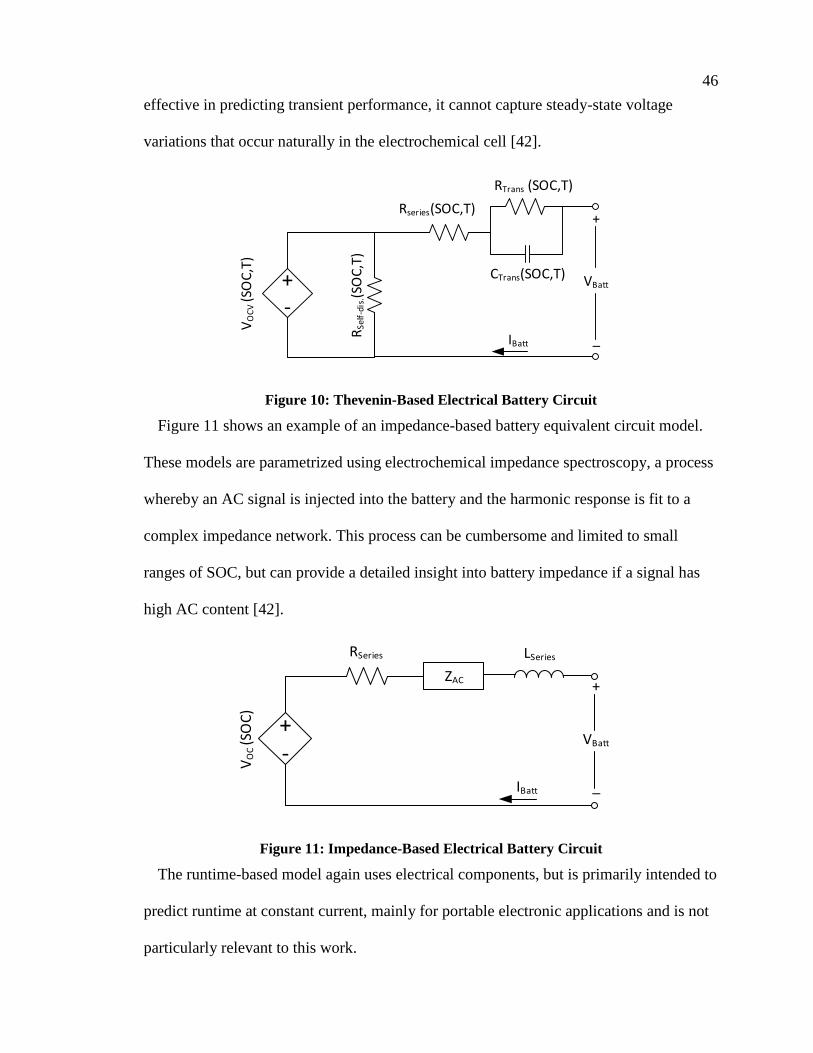
46

effective in predicting transient performance, it cannot capture steady-state voltage

variations that occur naturally in the electrochemical cell [42].

+-

VO

CV

(SO

C,T

)

RSe

lf-d

is.(S

OC

,T)

Rseries(SOC,T)

RTrans (SOC,T)

CTrans(SOC,T) VBatt

+

_IBatt

Figure 10: Thevenin-Based Electrical Battery Circuit

Figure 11 shows an example of an impedance-based battery equivalent circuit model.

These models are parametrized using electrochemical impedance spectroscopy, a process

whereby an AC signal is injected into the battery and the harmonic response is fit to a

complex impedance network. This process can be cumbersome and limited to small

ranges of SOC, but can provide a detailed insight into battery impedance if a signal has

high AC content [42].

+-

ZAC

RSeries LSeries

VO

C (S

OC

)

IBatt

+

_

VBatt

Figure 11: Impedance-Based Electrical Battery Circuit

The runtime-based model again uses electrical components, but is primarily intended to

predict runtime at constant current, mainly for portable electronic applications and is not

particularly relevant to this work.

47

The dual polarization Thevenin-based circuit has been shown to provide a good

representation for the Lithium Titanate Oxide (LTO) chemistry selected for the case

study [43]. Self-discharge can generally be neglected with this chemistry under normal

conditions, and thus the parallel resistance can be eliminated from the circuit.

HPPC testing is most commonly performed at the cell level; therefore, pack level

characteristics need to be scaled appropriately for the voltage and capacity requirements

of the pack. The equivalent impedance of the R-RC-RC circuit is given by,

𝑍𝑐𝑒𝑙𝑙,𝑒𝑞 = 𝑍𝑆𝑒𝑟𝑖𝑒𝑠 + 𝑍𝑅𝐶1 + 𝑍𝑅𝐶2 ( 2-41 )

Expanding the RC impedances we get,

𝑍𝑐𝑒𝑙𝑙,𝑒𝑞 = 𝑅𝑆,𝑐𝑒𝑙𝑙 +1

1𝑅1,𝑐𝑒𝑙𝑙

+ 𝑗𝜔𝐶1,𝑐𝑒𝑙𝑙

+1



( 2-42 )

𝑍𝑝𝑎𝑐𝑘,𝑒𝑞 = 𝑅𝑆,𝑝𝑎𝑐𝑘 +1

1𝑅1,𝑝𝑎𝑐𝑘

+ 𝑗𝜔𝐶1,𝑝𝑎𝑐𝑘

+1



( 2-43 )

For a pack consisting of 𝑛𝑠 cells in series, the impedance of the pack can be

analytically extrapolated using the following relationship,

𝑍𝑝𝑎𝑐𝑘,𝑒𝑞 = 𝑍𝑐𝑒𝑙𝑙,𝑒𝑞 + 𝑍𝑐𝑒𝑙𝑙,𝑒𝑞 +⋯ = 𝑛𝑠𝑍𝑐𝑒𝑙𝑙,𝑒𝑞 ( 2-44 )

The equivalent circuit parameters can be analytically related to pack level parameters

as follows:

1



=𝑛𝑠



=1

1𝑛𝑠𝑅1,𝑐𝑒𝑙𝑙

+ 𝑗𝜔𝐶1,𝑐𝑒𝑙𝑙𝑛𝑠

( 2-45 )

48

Therefore,

𝑅𝑆,𝑝𝑎𝑐𝑘 = 𝑛𝑠𝑅𝑆,𝑐𝑒𝑙𝑙 ( 2-46 )

𝑅𝑖,𝑝𝑎𝑐𝑘 = 𝑛𝑠𝑅𝑖,𝑐𝑒𝑙𝑙 ( 2-47 )

𝐶𝑖,𝑐𝑒𝑙𝑙 =𝐶𝑖,𝑐𝑒𝑙𝑙𝑛𝑠

( 2-48 )

An analytical expression can also be derived for cells in parallel. The impedance of

equivalent cell circuits in parallel is given by,

1

𝑍𝑝𝑎𝑐𝑘,𝑒𝑞=

1

𝑍𝑐𝑒𝑙𝑙,𝑒𝑞+

1

𝑍𝑐𝑒𝑙𝑙,𝑒𝑞+⋯ =

𝑛𝑠𝑍𝑐𝑒𝑙𝑙,𝑒𝑞

( 2-49 )

𝑍𝑝𝑎𝑐𝑘,𝑒𝑞 =𝑍𝑐𝑒𝑙𝑙,𝑒𝑞

𝑛𝑝

=1

𝑛𝑝[𝑅𝑆,𝑐𝑒𝑙𝑙 +

𝑅1,𝑐𝑒𝑙𝑙1 + 𝑗𝜔𝑅1,𝑐𝑒𝑙𝑙𝐶1,𝑐𝑒𝑙𝑙

+𝑅2,𝑐𝑒𝑙𝑙

1 + 𝑗𝜔𝑅2,𝑐𝑒𝑙𝑙𝐶2,𝑐𝑒𝑙𝑙]

( 2-50 )

Therefore,

𝑅𝑆,𝑝𝑎𝑐𝑘 =𝑅𝑆,𝑐𝑒𝑙𝑙𝑛𝑝

( 2-51 )

𝑅𝑖,𝑝𝑎𝑐𝑘 =𝑅𝑖,𝑐𝑒𝑙𝑙𝑛𝑝

( 2-52 )

𝐶𝑖,𝑐𝑒𝑙𝑙 = 𝑛𝑝𝐶𝑖,𝑐𝑒𝑙𝑙 ( 2-53 )

Scaling of cell parameters to pack level provides an initial estimate, but is known to not

be particularly accurate. This is because additional resistances from internal connections

points, laser welds, and other contact resistances can have a significant impact on the

overall impedance of the pack. Furthermore, pack internals can also produce additional

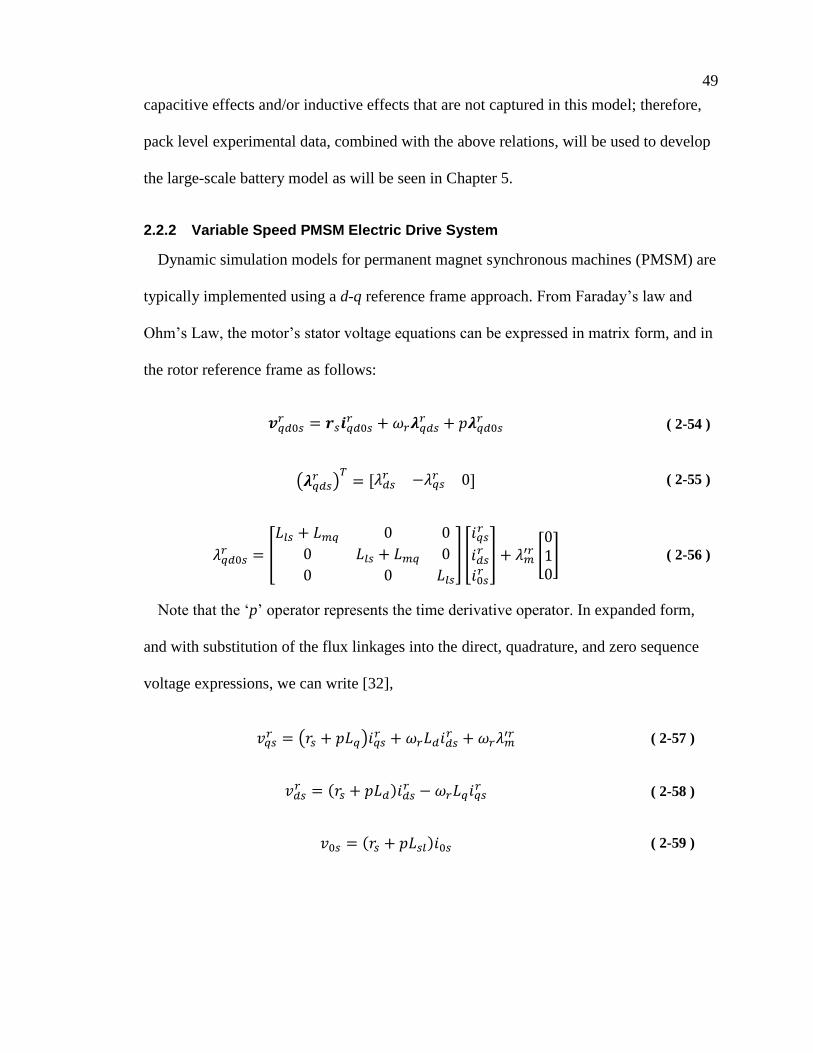
49

capacitive effects and/or inductive effects that are not captured in this model; therefore,

pack level experimental data, combined with the above relations, will be used to develop

the large-scale battery model as will be seen in Chapter 5.

2.2.2 Variable Speed PMSM Electric Drive System

Dynamic simulation models for permanent magnet synchronous machines (PMSM) are

typically implemented using a d-q reference frame approach. From Faraday’s law and

Ohm’s Law, the motor’s stator voltage equations can be expressed in matrix form, and in

the rotor reference frame as follows:

𝒗𝑞𝑑0𝑠𝑟 = 𝒓𝑠𝒊𝑞𝑑0𝑠

𝑟 + 𝜔𝑟𝝀𝑞𝑑𝑠𝑟 + 𝑝𝝀𝑞𝑑0𝑠

𝑟 ( 2-54 )

(𝝀𝑞𝑑𝑠𝑟 )

𝑇= [𝜆𝑑𝑠

𝑟 −𝜆𝑞𝑠𝑟 0] ( 2-55 )

𝜆𝑞𝑑0𝑠𝑟 = [

𝐿𝑙𝑠 + 𝐿𝑚𝑞 0 0

0 𝐿𝑙𝑠 + 𝐿𝑚𝑞 0

0 0 𝐿𝑙𝑠

] [

𝑖𝑞𝑠𝑟

𝑖𝑑𝑠𝑟

𝑖0𝑠𝑟

] + 𝜆𝑚′𝑟 [010] ( 2-56 )

Note that the ‘p’ operator represents the time derivative operator. In expanded form,

and with substitution of the flux linkages into the direct, quadrature, and zero sequence

voltage expressions, we can write [32],

𝑣𝑞𝑠𝑟 = (𝑟𝑠 + 𝑝𝐿𝑞)𝑖𝑞𝑠

𝑟 + 𝜔𝑟𝐿𝑑𝑖𝑑𝑠𝑟 + 𝜔𝑟𝜆𝑚

′𝑟 ( 2-57 )

𝑣𝑑𝑠𝑟 = (𝑟𝑠 + 𝑝𝐿𝑑)𝑖𝑑𝑠

𝑟 − 𝜔𝑟𝐿𝑞𝑖𝑞𝑠𝑟 ( 2-58 )

𝑣0𝑠 = (𝑟𝑠 + 𝑝𝐿𝑠𝑙)𝑖0𝑠 ( 2-59 )

50

The power output is conserved regardless of the coordinate frame; therefore, the power

equation for the electric machine can be expressed as,

𝑃𝑎𝑏𝑐𝑠 = 𝑃𝑑𝑞0 = 3

2(𝑣𝑞𝑠𝑖𝑞𝑠 + 𝑣𝑑𝑠𝑖𝑑𝑠 + 2𝑣0𝑠𝑖0𝑠) ( 2-60 )

Consequently, a simplified expression can be developed for torque generated by the

machine using energy conservation,

𝑃𝑚𝑎𝑐ℎ𝑖𝑛𝑒 = 𝑇𝑒𝜔𝑟 = 𝑇𝑒 (2

𝑃𝑛)𝜔𝑒 =

3

2(𝑣𝑞𝑠𝑖𝑞𝑠 + 𝑣𝑑𝑠𝑖𝑑𝑠 + 2𝑣0𝑠𝑖0𝑠) ( 2-61 )

Here 𝑃𝑛 denotes the number of pole pairs which relates the electrical frequency to the

mechanical rotor frequency. Substituting the stator equations into the power equation and

grouping like terms, the losses can be decomposed as follows,

𝑇𝑒 (2

𝑃)𝜔𝑟 =

3

2𝑟𝑠(𝑖𝑞𝑠𝑟

2 + 𝑖𝑑𝑠𝑟 2 + 2𝑖0𝑠

2)⏞

Ohmic Losses

+3

2(𝜆𝑑𝑠𝑟 𝑖𝑞𝑠𝑟 − 𝜆𝑞𝑠𝑟 𝑖𝑑𝑠

𝑟 )𝜔𝑟⏞

Torque Production

+3

2(𝑖𝑞𝑠𝑟 𝑝𝜆𝑞𝑠

𝑟 + 𝑖𝑑𝑠𝑟 𝑝𝜆𝑑𝑠

𝑟 + 2𝑖0𝑠𝑝𝜆0𝑠)⏟ Stored Magnetic Energy

( 2-62 )

Ohmic losses and stored magnetic energy terms impact the mechanical output torque

generated. The electromagnetic torque produced by the machine is given by,

𝑇𝑒 = (3

2) (𝑃

2) (𝜆𝑑𝑠

𝑟 𝑖𝑞𝑠𝑟 − 𝜆𝑞𝑠

𝑟 𝑖𝑑𝑠𝑟 ) ( 2-63 )

The d-q flux linkages can be substituted to get an expression for torque production based

on the input stator current,

51

𝑇𝑒 = (3

2) (𝑃

2) ((𝐿𝑑𝑖𝑑𝑠

𝑟 + 𝜆𝑚′𝑟)𝑖𝑞𝑠

𝑟 − (𝐿𝑞𝑖𝑞𝑠𝑟 )𝑖𝑑𝑠

𝑟 )

= (3

2) (𝑃

2) (𝜆𝑚

′𝑟𝑖𝑞𝑠𝑟 + (𝐿𝑑 − 𝐿𝑞)𝑖𝑞𝑠

𝑟 𝑖𝑑𝑠𝑟 )

( 2-64 )

Note that 𝜆𝑚′𝑟 represents the flux established by the permanent magnets. The PMSM

model to this point has only considered copper losses through resistive dissipation in the

stator coils. This model can be augmented to include other physical sources of energy

dissipation including iron losses, and magnetic saturation effects. In this work, iron losses

will be also be considered and the equivalent circuit type representation of the PMSM is

shown in Figure 12.

rs

ri Ld

- +

ωrLqriqs

r

vd

rs

ri Lq

+ -

ωrLdrids

r

vq

+ -

ωr λ'mr

rs

Ld

- +

ωrLqriqs

r

vd

rs

Lq

+ -

ωrLdrids

r

vq

+ -

ωr λ'mr

+

-

+

-

+

-

+

-

Figure 12: PMSM Equivalent Circuit including Iron Loss

The inclusion of iron losses reduces the amount of useful current delivered to the

magnetic circuit. At steady state, the time derivative in the d-q stator voltage equations

trend to zero and the equations reduce to [34],

52

𝑣𝑞𝑠𝑟 = 𝑟𝑠𝑖𝑞𝑠

𝑟 + (1 +𝑟𝑠𝑟𝑖) (𝜔𝑟𝐿𝑑𝑖𝑑𝑠

𝑟 + 𝜔𝑟𝜆𝑚′𝑟) ( 2-65 )

𝑣𝑑𝑠𝑟 = 𝑟𝑠𝑖𝑑𝑠

𝑟 − (1 +𝑟𝑠𝑟𝑖)𝜔𝑟𝐿𝑞𝑖𝑞𝑠

𝑟 ( 2-66 )

Because the three phases are balanced, the zero sequence equation equals zero. The

inclusion of both iron and copper losses will provide two parameters that can help tune

the model to represent the published performance data. The aggregate sum of these losses

can be simulated to dynamically estimate electric machine efficiency when coupled with

a motor drive.

2.2.2.1 Inverter and Drive System

A voltage source inverter (VSI) is one of the most commonly encountered switching

converters used in traction drive applications. In an AES applications, VSI drives are

often preferred because of their near unity power factor on the AC distribution system

[2]. The alternate drive configuration for an AC motor is the current source inverter (CSI)

whose details are not discussed here. The interested reader can find details on the CSI in

Krause [32], Adnanes [81], and Hansen [2].

The commercial motor selected for the case study uses a VSI with Space Vector Pulse

Width Modulation (SVPWM). In order to construct an average value model

representation suitable for system-level simulation, a dynamic averaging technique must

be implemented to eliminate the need to resolve switching devices, yet preserve the

dominant converter dynamics. The PMSM motor and VSI drive circuit is presented in

Figure 13.

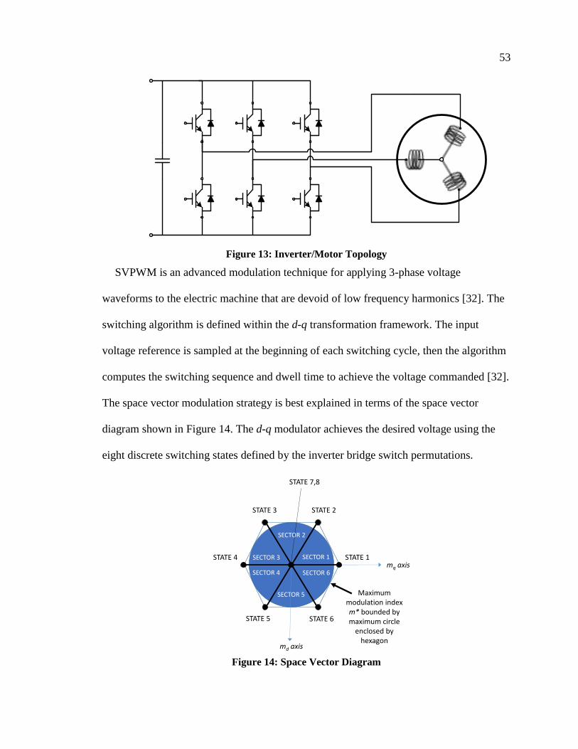
53

Figure 13: Inverter/Motor Topology

SVPWM is an advanced modulation technique for applying 3-phase voltage

waveforms to the electric machine that are devoid of low frequency harmonics [32]. The

switching algorithm is defined within the d-q transformation framework. The input

voltage reference is sampled at the beginning of each switching cycle, then the algorithm

computes the switching sequence and dwell time to achieve the voltage commanded [32].

The space vector modulation strategy is best explained in terms of the space vector

diagram shown in Figure 14. The d-q modulator achieves the desired voltage using the

eight discrete switching states defined by the inverter bridge switch permutations.

Figure 14: Space Vector Diagram

STATE 3 STATE 2

STATE 1

STATE 6STATE 5

STATE 4 SECTOR 1

SECTOR 2

SECTOR 3

SECTOR 4

SECTOR 5

SECTOR 6 mq axis

md axis

STATE 7,8

Maximum modulation index m* bounded by maximum circle

enclosed by hexagon

54

A more comprehensive treatment of the SVPWM strategy can be found in Krause [32].

Insight into the low-level switching behaviour is necessary for establishing a time-

averaged simulation model as will be seen in the following section. Verification of any

average value models must include comparison against a detailed simulation where the

exact switching pattern of the inverter bridge based is modeled.

In control synthesis of VSI drives, the dynamics of the converter bridge can be

modeled as a first order transfer function with a time constant equal to that of the

switching frequency period Krishnan [33] or,

𝐺𝑐𝑜𝑛𝑣(𝑠) =1

𝜏𝑠𝑠 + 1 ( 2-67 )

A time-averaged dynamic loss model for the semiconductors of the VSI can be

developed with insight into the SVPWM switching cycles and current waveforms. In the

work of Bierhoff and Fuchs [38], the authors develop an analytical expression for the

total bridge losses associated with a SVPWM switching strategy. The total energy losses

from the inverter bridge consists of switching losses in turn-on and turn-off, as well as

conduction losses from switching devices and freewheel diodes. The total energy loss for

a pair of switches is given by,

𝐼𝑛𝑣,𝑙𝑜𝑠𝑠 = 𝑠𝑙 + 𝑐𝑙,𝐼 + 𝑐𝑙,𝐷 ( 2-68 )

where,

Total

Switching

Loss:

𝑠𝑙 =𝑓𝑠𝜋(𝐸𝑜𝑛,𝐼 + 𝐸off,𝐼 + 𝐸off,𝐷)

𝑉𝐷𝐶𝑉𝑟𝑒𝑓

∙𝐼𝐿𝐼𝑟𝑒𝑓

( 2-69 )

55

IGBT

Conduction

Loss: 𝑐𝑙,𝐼 =

𝑉𝐶𝐸,0𝐼𝐿2𝜋

[1 +𝑀𝜋

4cos(𝛿)] +

𝑅𝐶𝐸𝐼𝐿2

2𝜋[𝜋

4+2

3𝑀 cos(𝛿)] ( 2-70 )

Diode

Conduction

Loss: 𝑐𝑙,𝐷 =

𝑉𝐹,0𝐼𝐿2𝜋

[1 −𝑀𝜋

4cos(𝛿)] +

𝑅𝐹𝐼𝐿2

2𝜋[𝜋

4−2

3𝑀 cos(𝛿)] ( 2-71 )

The parameters are given by,

𝑉𝑟𝑒𝑓 Reference voltage for switching energy loss

𝐼𝑟𝑒𝑓 Reference current for switching energy loss

𝑓𝑠 Carrier switching frequency

𝑉𝐷𝐶 DC source voltage

𝐼𝐿 Peak value of the AC line current (assumed sinusoidal)

𝐸𝑜𝑛,𝐼 IGBT turn-on switching energy losses

𝐸off,𝐼 IGBT turn-off switching energy loss

𝐸off,𝐷 Diode turn-off switching energy loss

𝑀 Modulation index

𝑉𝐶𝐸,0 Threshold voltage across collector/emitter for IGBT in on-state

𝑅𝐶𝐸 Differential resistance of IGBT in on-state

𝑉𝐹,0 Threshold voltage across collector/emitter for diode in on-state

𝑅𝐹 Differential resistance of diode in on-state

𝛿 Displacement angle between fundamental voltage and load current

These equations were also used in Chao et al. [34] to develop efficiency maps for

PMSM electric drive systems. We can therefore make an approximation for the energy

losses in the inverter bridge as part of our simulation model using information contained

within semiconductor datasheets with similar power ratings; however, the modulation

index and displacement angle of the load must be computed as part of the AVM.

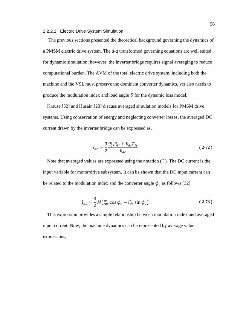
56

2.2.2.2 Electric Drive System Simulation

The previous sections presented the theoretical background governing the dynamics of

a PMSM electric drive system. The d-q transformed governing equations are well suited

for dynamic simulation; however, the inverter bridge requires signal averaging to reduce

computational burden. The AVM of the total electric drive system, including both the

machine and the VSI, must preserve the dominant converter dynamics, yet also needs to

produce the modulation index and load angle 𝛿 for the dynamic loss model.

Krause [32] and Husain [23] discuss averaged simulation models for PMSM drive

systems. Using conservation of energy and neglecting converter losses, the averaged DC

current drawn by the inverter bridge can be expressed as,

𝑖𝑑𝑐 =3

2

𝑣𝑞𝑠𝑟 𝑖𝑞𝑠𝑟 + 𝑣𝑑𝑠

𝑟 𝑖𝑑𝑠𝑟

𝑣𝑑𝑐 ( 2-72 )

Note that averaged values are expressed using the notation ( ∙ ). The DC current is the

input variable for motor/drive subsystem. It can be shown that the DC input current can

be related to the modulation index and the converter angle 𝜙𝑣 as follows [32],

𝑖𝑑𝑐 =3

2𝑀(𝑖𝑞𝑠

𝑟 cos𝜙𝑣 − 𝑖𝑑𝑠𝑟 sin𝜙𝑣) ( 2-73 )

This expression provides a simple relationship between modulation index and averaged

input current. Now, the machine dynamics can be represented by average value

expressions,

57

𝑝𝑖𝑞𝑠𝑟 =

𝑣𝑞𝑠𝑟 − 𝑟𝑠𝑖𝑞𝑠

𝑟 − 𝜔𝑟𝐿𝑑𝑖𝑑𝑠𝑟 − 𝜔𝑟𝜆𝑚

′

𝐿𝑞 ( 2-74 )

𝑝𝑖𝑑𝑠𝑟 =

𝑣𝑑𝑠𝑟 − 𝑟𝑠𝑖𝑑𝑠

𝑟 + 𝜔𝑟𝐿𝑞𝑖𝑞𝑠𝑟

𝐿𝑑 ( 2-75 )

The rotational frequency is assumed to be varying slowly as compared to the switching

cycle; therefore, angular velocity can be considered constant over the averaging period.

SVPWM provides a low-ripple torque output as a result of eliminating low frequency

harmonics; therefore, the averaged torque can be written as,

𝑒 =3

2

𝑃

2(𝜆𝑚′ 𝑖𝑞𝑠

𝑟 + (𝐿𝑑 − 𝐿𝑞)𝑖𝑞𝑠𝑟 𝑖𝑑𝑠

𝑟 ) ( 2-76 )

Note, the preceding discussion also assumes that the DC bus voltage is constant or

slowly varying as compared with switching frequency. This assumption is valid

considering that the DC bus voltage is regulated. The overall simulation model

information flow can be described by the block diagram in Figure 15.

Figure 15: PMSM Drive AVM Block Diagram

2.2.3 Power Converter Modeling

AES architectures can consist of multiple types of power converters that convert

between fixed frequency AC, variable frequency AC, and DC power supplies. Typical

marine power converters are comprised of semiconductor devices including diodes,

thyristors, SCRs, IGBTs, etc. depending on the application. A comprehensive overview

of marine power electronic converters can be found in Adnanes [81], but detailed

VSIDRIVE

MODEL

PMSMMOTORMODEL

58

treatment of this subject is beyond the scope of this work. A DC grid distribution system

will be modeled for this case study, which inherently requires a power converter interface

for all system components that attached to the bus. The interfacing converters are

required for the several reasons:

Control of harmonic content on DC distribution bus

DC voltage regulation

Fault mitigation and control

Supervisory system control

Power converters are non-linear systems that require special attention. The previous

section discussed average value modeling of a VSI converter in the context of developing

a simulation model for the main propulsion motors. The switching dynamics of power

converters are extremely fast relative to ship motion; therefore, much of the high

frequency dynamics can be neglected for the present objectives. Moving forward into the

SIL platform development, averaged value models for the other switching converters will

be developed following the approach of Zahedi and Norum [26].

The BEIPS architecture requires a model for the main high power bi-directional

DC/DC converter, which interfaces the battery-based energy storage system. In addition,

a DC/AC islanding converter is required for servicing the AC hotel loads. For these

converters, a simplified power loss modeling approach will be used to capture losses, but

dynamics will be ignored. The efficiency is given as a function of the power requested as

shown in Figure 16.

59

Figure 16: Power Loss Model for Converters

The islanding converter is unidirectional and its implementation is straightforward. The

DC/DC converter is bi-directional; therefore, its implementation requires some additional

functionality to account for losses when power flow is reversed. Unlike most AES

applications that include energy storage, the DC/DC converter will be used to regulate the

DC grid bus voltage in the absence of an electrical generation system. In this type of

system, battery current is manipulated as the control variable in both buck and boost

mode. The detailed implementation is discussed in Chapter 5.

2.2.4 Lithium-Ion Battery Rapid Charging

The BEIPS concept under investigation is intended to use frequent fast-charging cycles

to replenish the energy consumed during a single crossing; therefore, a model of the

charging infrastructure is required for inclusion in the simulation. The intent is to

investigate the use of rapid-charging cycles during each load/unload periods, at both

terminals. The charging process for lithium-ion batteries begins with a constant current

(CC) supply which is held until the maximum rated battery voltage is reached. At this

point, the charger switches to a constant voltage (CV) and the current gradually decays to

zero. This is referred to a CC/CV charging cycle. The process is illustrated graphically in

Figure 17.

Pout

Pinη(Pin)

η

Multiply

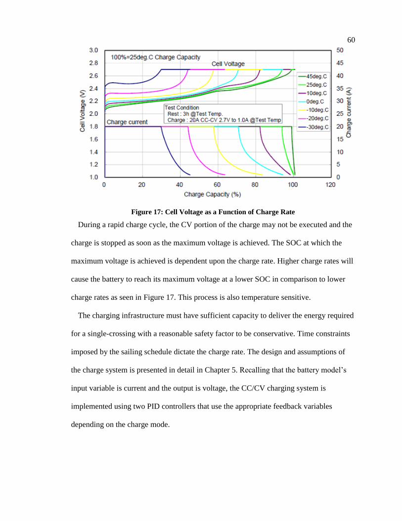
60

Figure 17: Cell Voltage as a Function of Charge Rate

During a rapid charge cycle, the CV portion of the charge may not be executed and the

charge is stopped as soon as the maximum voltage is achieved. The SOC at which the

maximum voltage is achieved is dependent upon the charge rate. Higher charge rates will

cause the battery to reach its maximum voltage at a lower SOC in comparison to lower

charge rates as seen in Figure 17. This process is also temperature sensitive.

The charging infrastructure must have sufficient capacity to deliver the energy required

for a single-crossing with a reasonable safety factor to be conservative. Time constraints

imposed by the sailing schedule dictate the charge rate. The design and assumptions of

the charge system is presented in detail in Chapter 5. Recalling that the battery model’s

input variable is current and the output is voltage, the CC/CV charging system is

implemented using two PID controllers that use the appropriate feedback variables

depending on the charge mode.

61

2.3 Vessel Dynamics Modeling

2.3.1 Ship Dynamics Modeling

To this point we have addressed the background relating to modeling and simulation of

the IPS components and thrust production. The last major remaining sub-section of the

plant model is the representation of the ship motion dynamics in response to

environmental and actuator forces. The detailed physics that govern vessel motion are

represented by complex fluid mechanics, making the vehicle dynamics model for marine

applications significantly more involved than in automotive studies; however, the

dynamic response of ships has been studied extensively in classical marine literature

through seakeeping and maneuvering analyses. This foundation provides the theoretical

basis for development of parametric vessel model.

Seakeeping analysis is generally conducted to investigate the vessel’s response to

sinusoidal excitation while traveling at constant course and constant speed. This type of

analysis is used primarily to predict the induced motion from wave excitation.

Maneuvering theory, on the other hand, is conducted assuming no waves are present, and

the focus lies in studying the vessel’s trajectory and response when executing a

prescribed maneuver.

In this work, the objective is to develop a holistic framework that can account for

propulsive effects during both free motion at different sea states. Application of unified

seakeeping/maneuvering theory discussed by Fossen [63] provides a foundational

structure for developing the vessel’s dynamic equations. This section provides a summary

of the relevant theory relating to floating body dynamics, and introduces the Marine

Systems Simulator (MSS) toolbox developed by Perez and Fossen [78] that will be used

in the development.

62

2.3.2 Coordinate System Definitions and Notation

One of the major differences between the seakeeping and maneuvering analysis

involves the choice of inertial coordinate system. We will define the global inertial frame

using the North-East-Down convention. Displacements with respect to the inertial frame

are represented by the position vector,

𝜼 = [𝑁 𝐸 𝐷 𝜙 𝜃 𝜓]𝑇 ( 2-77 )

In both seakeeping and maneuvering studies, a body-fixed coordinate system is defined

for convenience, largely because hydrodynamic coefficients are generally referenced to

this frame. The instantaneous velocity of the ship in the body-fixed frame is denoted as,

𝝂 = [𝑢 𝑣 𝑤 𝑝 𝑞 𝑟]𝑇 ( 2-78 )

where, 𝑢 is velocity in surge

𝑣 is velocity in sway

𝑤 is velocity in heave

𝑝 is angular velocity of roll

𝑞 is angular velocity of pitch

𝑟 is angular velocity of yaw

In seakeeping analysis, another reference frame is defined to represent the equilibrium

position of the ship traveling at a constant speed and at a constant course. This represents

the equilibrium position of the ship in the absence of waves. For a given heading angle ,

the seakeeping frame is expressed in the NED inertial coordinates by,

𝝊𝒔/𝒏𝒏 = [𝑈 cos 𝑈 sin 0]𝑇 ( 2-79 )

Motion and displacements relative to the equilibrium are defined using relative motion

analysis. Perturbation coordinates are used to define relative displacement relative to the

seakeeping frame.

63

𝛿𝜼 = [𝒓𝒃/𝒔𝒔

𝚯𝒔𝒃] ( 2-80 )

𝒓𝒃/𝒔𝒔 = [𝛿𝑥 𝛿𝑦 𝛿𝑧]𝑇 ( 2-81 )

𝚯𝒔𝒃 = [𝛿𝜃 𝛿𝜙 𝛿𝜓]𝑇 ( 2-82 )

Velocity perturbations, expressed in body-fixed frame are defined as,

𝛿𝝂 = [𝛿𝝂𝟏𝛿𝝂𝟐

] = [[𝛿𝑢 𝛿𝑣 𝛿𝑤]𝑇

[𝛿𝑝 𝛿𝑞 𝛿𝑟]𝑇] ( 2-83 )

Coordinates in the body-fixed frame can be transformed into the seakeeping frame

using a transformation defined by the Euler angle transformation matrix. It is critical to

highlight a key distinction between seakeeping coordinates and generalized coordinates

for maneuvering models. We define,

= 𝑱𝚯(𝜼)𝝂 ( 2-84 ) ⇒ Coordinate transformation from body-fixed

frame to NED inertial frame

𝛿 = 𝑱𝚯(𝛿𝜼)𝛿𝝂 ( 2-85 ) ⇒ Coordinate transformation from body-fixed

frame to seakeeping frame

A detailed explanation of the 𝐽Θ transformation matrix can be found in [63] and is

presented here without explanation. The objective now is to develop a linear

transformation to allow for transition between seakeeping perturbations coordinates

(𝛿𝝂, 𝛿𝜼) to body fixed-NED coordinates (𝝂, 𝜼). If we consider a ship moving at constant

speed and constant course about its equilibrium position, the velocity of the ship in body-

fixed frame is expressed as the sum of the average velocity and the perturbation velocity,

𝝂𝟏 = 𝟏 + 𝛿𝝂𝟏 ( 2-86 )

Using relative motion analysis and assuming small angular displacements, the average

velocity 𝟏 can be approximated by [63],

64

𝟏 = 𝑈 [

cos 𝛿𝜓 cos 𝛿𝜃− sin 𝛿𝜓 cos 𝛿𝜙 + cos 𝛿𝜓 sin 𝛿𝜃 sin 𝛿𝜙sin 𝛿𝜓 sin 𝛿𝜙 + cos 𝛿𝜓 cos 𝛿𝜙 sin 𝛿𝜃

] ≈ 𝑈 [1

−𝛿𝜓𝛿𝜃

] ( 2-87 )

The average angular velocity in roll, pitch, and yaw is assumed to be zero; therefore,

we can write,

𝝂 = + 𝛿𝝂 ( 2-88 ) where, ≈ 𝑈[1 −𝛿𝜓 𝛿𝜃 0 0 0]𝑇 ( 2-89 )

By defining the vector 𝒆𝟏 and matrix 𝑳 as follows,

𝒆𝟏 ≡

[ 100000]

( 2-90 ) and, 𝑳 ≡

[ 0 0 0 0 0 00 0 0 0 0 10 0 0 0 −1 00 0 0 0 0 00 0 0 0 0 00 0 0 0 0 0]

( 2-91 )

Fossen [63] writes the velocity expressions given by Equation ( 2-88 ) and Equation (

2-89 ) in matrix form,

𝝂 ≈ 𝑈(𝒆𝟏 − 𝐿𝛿𝜼) + 𝛿𝝂 ( 2-92 )

From this expression, the perturbations velocities and accelerations expressed in body-

fixed frame as [63],

𝛿𝝂 ≈ 𝝂 + 𝑈(𝑳𝛿𝜼 − 𝒆𝟏) ( 2-93 )

𝛿 ≈ + 𝑈(𝑳𝛿𝝂) = + 𝑈𝑳(𝝂 + 𝑈(𝑳𝛿𝜼 − 𝒆𝟏)) ( 2-94 )

The Euler angles relating the seakeeping perturbations coordinates (𝛿𝝂, 𝛿𝜼) to NED

coordinates is given by,

65

[𝜙𝜃𝜓] = [

00] + [

𝛿𝜙𝛿𝜃𝛿𝜓] ( 2-95 )

This is an important result for unifying maneuvering and seakeeping theory into a

single model; however, there is a range of applicability for this type of formulation. The

above relationships assume perturbations about a cruise velocity 𝑈 which works well for

in-transit analysis; however, this definition can breakdown with large scale perturbations

or significant changes in forward speed.

2.3.3 Seakeeping Analysis and the Classical Frequency-Domain Model

Seakeeping analysis is typically conducted in the frequency domain assuming

harmonic excitation. In classical hydrodynamic literature, the formulation of the

equations of motion are constructed within a linear framework under the assumption that

forces can be summed using superposition. It is often convenient for notational simplicity

to replace perturbation notation with a change of variable for time domain equations,

𝝃 = 𝛿𝜼 ( 2-96 )

The equations of motion governing a floating structure undergoing forced oscillations

are expressed as follows,

𝑴𝑅𝐵 = 𝑴𝑅𝐵𝛿 = 𝛿𝝉𝑹𝑩 ( 2-97 )

where, = 𝛿𝝂 ( 2-98 )

𝑴𝑅𝐵 =

[ 𝑚 0 0 0 0 00 𝑚 0 0 0 00 0 𝑚 0 0 00 0 0 𝐼𝑥𝑥 𝐼𝑥𝑦 𝐼𝑥𝑧0 0 0 𝐼𝑦𝑥 𝐼𝑦𝑦 𝐼𝑦𝑧0 0 0 𝐼𝑧𝑥 𝐼𝑧𝑦 𝐼𝑧𝑧]

( 2-99 )

66

The sum of forces acting on the body is decomposed into three components,

𝝉𝑅𝐵 = 𝝉ℎ𝑦𝑑 + 𝝉ℎ𝑠 + 𝝉𝑒𝑥𝑐 ( 2-100 )

The excitation forces imposed on the body are captured by 𝝉𝑒𝑥𝑐. The hydrostatic forces

from the vessel’s displacement is encompassed in the vector 𝝉ℎ𝑠. Lastly, the

hydrodynamic forces imposed by the fluid as result of the motion are represented by

𝝉ℎ𝑦𝑑. Cummins [61] showed that the hydrodynamic radiation forces acting on a body

subjected to forced oscillation in an inviscid fluid can be expressed by,

𝝉𝑟𝑎𝑑 = −𝑨∞ + ∫ 𝑲𝑡

0

(𝑡 − 𝜅)(𝑡)𝑑𝜅 ( 2-101 )

The term 𝑨∞ represents the added mass at infinite frequency. The term 𝑲(𝑡) is a

matrix of retardation functions that capture the time-history of impulse forces arising

from the disturbed water surface as a result of ship motion [61]. Using an inverse Fourier

transform, the retardation function can be defined as a function of frequency-dependent

damping coefficients [61],

𝑲(𝑡) =2

𝜋∫ 𝑩(𝜔)∞

0

cos (𝜔𝑡)𝑑𝜔 ( 2-102 )

Hydrodynamic solvers compute added mass and damping coefficients as function of

frequency. This can in turn be used to numerically solve for 𝑲(𝑡); however, the coming

sections will illustrate an alternate approach using state space transfer function fitting for

increased computational efficiency.

Substituting the expressions for hydrodynamic and hydrostatic forces into the Equation

( 2-97 ), the linear time-domain equation of motion for forced oscillation is,

67

[𝑴𝑅𝐵 + 𝑨∞](𝑡) + ∫ 𝑲(𝑡 − 𝜅)(𝑡)𝑑𝜅𝑡

0

+ 𝑪𝝃(𝑡) = 𝝉𝑒𝑥𝑐 ( 2-103 )

The matrix 𝑪 represents the hydrostatic forces resulting from displacement of the body.

When the excitation forces are considered to be sinusoidal and at a constant frequency,

the time-domain equation can be transformed into frequency-domain [63], [66], [62].

(−𝜔2[𝑴 + 𝑨(𝜔)] − 𝑗𝜔𝑩(𝜔) + 𝑪)(𝑗𝜔) = 𝑒𝑥𝑐(𝑗𝜔) ( 2-104 )

Hydrodynamic codes employ 3D potential flow solvers or 2D strip theory to compute

the added mass coefficients 𝑨(𝜔) and damping coefficients 𝑩(𝜔) for the linear equation

of motion at a specified vector of discrete frequencies. It is essential to note that the

damping coefficients from the hydrodynamic code only represent potential damping, and

do not consider viscous effects that are present in a real fluid. Additional resistive terms

are added to account for these effects as discussed in section 2.3.5.

The classical frequency domain equation derived uses perturbation coordinates from

the inertial seakeeping frame. As we move towards development of a unified

seakeeping/maneuvering model, it is more convenient to express equations in the body-

fixed frame. Substituting equations ( 2-93 ) and ( 2-94 ) into the time domain equation of

motion ( 2-103 ) [63],

[𝑴𝑅𝐵 + 𝑨∞]( + 𝑈𝑳𝝂) + ∫ 𝑲(𝑡 − 𝜅)[𝝂 − 𝑈𝒆1]𝑑𝜅𝑡

0

+ 𝑪𝜼 = 𝝉𝑒𝑥𝑡 ( 2-105 )

Note that the Ogilvie formulation for the retardation function, which provides greater

stability for numerical evaluation, has not been applied because the retardation function

will be estimated using a transfer function fitting approach. The reader is directed to [82]

68

and [63] for details. Finally, it is convenient to expand the first term and lump like terms

for further simplification to reach the time domain seakeeping equation,

𝑴 + 𝑪∗𝝂 + ∫ 𝑲(𝑡 − 𝜏)[𝝂 − 𝑈𝒆1]𝑑𝜏𝑡

0

+ 𝑮𝜼 = 𝝉𝑒𝑥𝑡𝑒𝑟𝑛𝑎𝑙 ( 2-106 )

where, 𝑴 = 𝑴𝑹𝑩 + 𝑨∞ ( 2-107 )

𝑪∗ = 𝑪𝑹𝑩∗ + 𝑪𝑨

∗ = (𝑈𝑴𝑹𝑩𝑳 + 𝑈𝑨∞𝑳) ( 2-108 )

Note that the hydrostatic stiffness matrix variable has been replaced to differentiate

between Coriolis matrix terms. This linearized model does not consider the forward

speed ship resistance, and assumes negligible perturbations in surge; therefore, a forward-

speed resistive force model must be developed in matrix form to account for these

effects. Treatment of forward speed effects is best done in the context of maneuvering.

2.3.4 Unified Seakeeping/Maneuvering Analyses for Vessel Dynamics Model

To this point, the matrix formulation of the equations of motion have only considered

perturbation about an equilibrium point moving at constant speed and constant course.

The resistive forces required to achieve the forward speed of the seakeeping frame are

unaccounted for, thus this framework must be augmented to include the ship’s forward

speed resistance. Furthermore, the objective is to develop a model that can predict

induced powertrain loads for a freely maneuvering ship; therefore, a maneuvering model

must be selected to account for non-linear drag effects.

Though maneuvering models have been studied extensively in academic literature,

these models have not demonstrated a high level accuracy. Bertram [68] discusses the

69

maturity levels of traditional maneuvering models and their limited success in

comparison to seakeeping models and other vessel motion analysis techniques.

The selection of the maneuvering model depends on the design problem at hand. Three

degree of freedom (DOF) surge-sway-yaw- models are the most common and widely

used for simple maneuvering studies [63]; however, more accurate models have been

developed to include the influence of roll [71]. Auto-pilot models can be as simple as a

single DOF system, such as the second order yaw Nomoto system [83]. Referring back to

the case study, the Klitsa is equipped with azimuthing propellers in a unique and highly

maneuverable configuration, eliminating the classic rudder arrangement upon which

maneuvering theory is generally founded. The barge-type hull is highly stable, so the roll

subsystem will have minimal impact on its maneuvering characteristics; therefore, a 3-

DOF model is appropriate for capturing the dominant dynamics.

One of the most widely used maneuvering models is the non-linear model of Abkowitz

[69] which uses a 3rd order truncated Taylor series expansion of the maneuvering

coefficients in the surge-sway-yaw systems. Bertram presents a set of non-

dimensionalized maneuvering coefficients for various vessel classes for parameterization

of the Abkowtiz non-linear model [68]. The Abkowitz model was developed primarily

for ships with the following characteristics:

Defined bow and stern

Propeller(s) at the stern

Rudder steering system

Many other maneuvering models have been developed over the years including work

by Fedyaevsky and Sobolev [84], Norrbin [85], Nomoto [83], Ross [71], and more, which

70

require experimental model data for parameterization. In this work, the 3-DOF model

based on surge resistance and cross-flow drag discussed in Fossen [63], has been selected

for its ease of implementation in the absence of maneuvering coefficient data.

Returning back to Equation ( 2-106 ), the system is augmented to include the

unaccounted resistive terms using a linear damping matrix 𝑫𝑳, and non-linear damping

matrix 𝑫𝑵.

𝑴 + 𝑪∗𝝂 + 𝑫𝑳𝝂 + 𝑫𝑵(𝝂) + ∫ 𝑲(𝑡 − 𝜅)[𝝂 − 𝑈𝒆1]𝑑𝜅𝑡

0

+ 𝑮𝜼 = 𝝉𝑒𝑥𝑡𝑒𝑟𝑛𝑎𝑙 ( 2-109 )

where,

𝑫𝑳 =

[ −𝑋𝑢 0 0 0 0 00 −𝑌𝑣 0 0 0 −𝑌𝑟0 0 0 0 0 00 0 0 0 0 00 0 0 0 0 00 −𝑁𝑣 0 0 0 −𝑁𝑟]

( 2-110 )

𝑫𝑵 =

[

1 2⁄ 𝜌𝑆(1 + 𝑘)𝐶𝑓𝑛𝑒𝑤(𝑢) ∙ |𝑢|𝑢

1

2𝜌∫ 𝑇(𝑥)𝐶𝑑

2𝐷(𝑥)|𝑣 + 𝑥𝑟|(𝑣 + 𝑥𝑟)𝑑𝑥𝐿𝑝𝑝/2

−𝐿𝑝𝑝 2⁄

000

1


2𝐷(𝑥)𝑥|𝑣 + 𝑥𝑟|(𝑣 + 𝑥𝑟)𝑑𝑥𝐿𝑝𝑝/2

−𝐿𝑝𝑝 2⁄ ]

( 2-111 )

With the addition of damping terms, this linearized integro-differential equation now

includes both seakeeping terms and a 3-DOF non-linear maneuvering model to

summarize the vessel dynamics. A discussion of parameterization and a detailed

explanation of the viscous components of resistance are provided in the following

section.

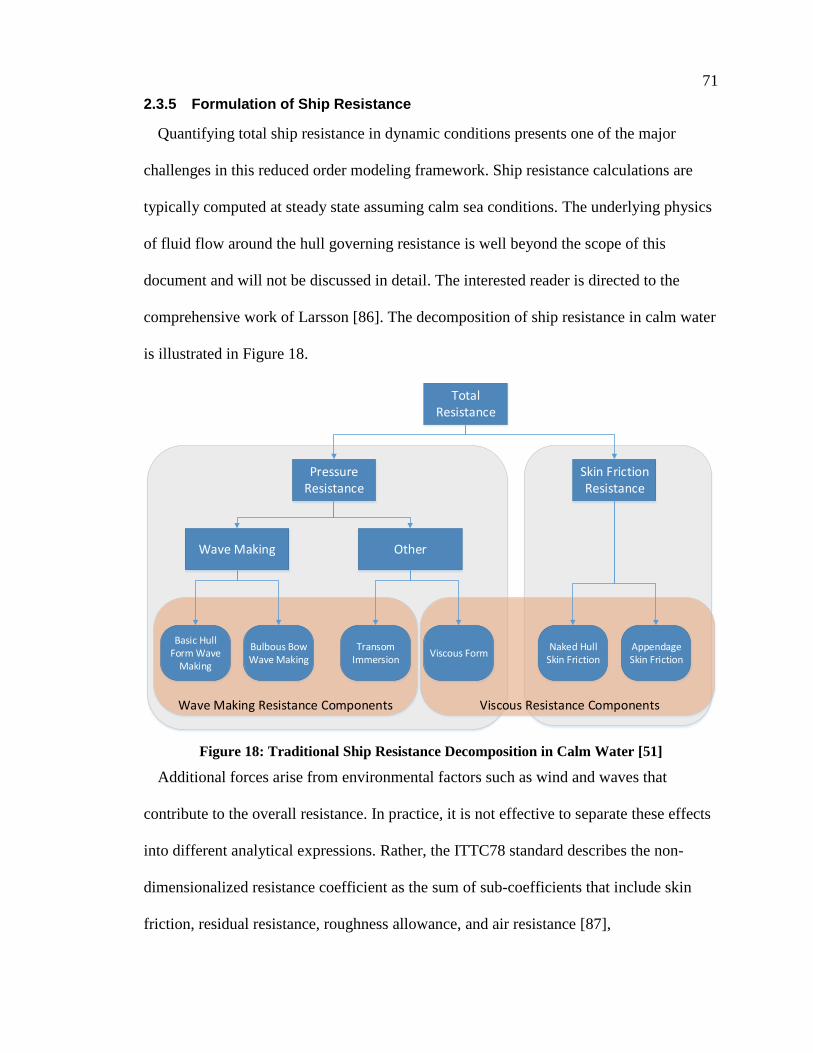
71

2.3.5 Formulation of Ship Resistance

Quantifying total ship resistance in dynamic conditions presents one of the major

challenges in this reduced order modeling framework. Ship resistance calculations are

typically computed at steady state assuming calm sea conditions. The underlying physics

of fluid flow around the hull governing resistance is well beyond the scope of this

document and will not be discussed in detail. The interested reader is directed to the

comprehensive work of Larsson [86]. The decomposition of ship resistance in calm water

is illustrated in Figure 18.

Total Resistance

Pressure Resistance

Skin Friction Resistance

Wave Making

Basic Hull Form Wave

Making

Bulbous Bow Wave Making

Transom Immersion

Viscous Form Naked Hull

Skin FrictionAppendage Skin Friction

Other

Wave Making Resistance Components Viscous Resistance Components

Figure 18: Traditional Ship Resistance Decomposition in Calm Water [51]

Additional forces arise from environmental factors such as wind and waves that

contribute to the overall resistance. In practice, it is not effective to separate these effects

into different analytical expressions. Rather, the ITTC78 standard describes the non-

dimensionalized resistance coefficient as the sum of sub-coefficients that include skin

friction, residual resistance, roughness allowance, and air resistance [87],

72

𝐶𝑇 = (1 + 𝑘)𝐶𝐹⏟ 𝑉𝑖𝑠𝑐𝑜𝑢𝑠𝐹𝑟𝑖𝑐𝑡𝑖𝑜𝑛

𝐶𝑜𝑒𝑓𝑓𝑖𝑐𝑖𝑒𝑛𝑡

+ 𝐶𝑅⏟𝑅𝑒𝑠𝑖𝑠𝑢𝑎𝑙𝑅𝑒𝑠𝑖𝑠𝑡𝑎𝑛𝑐𝑒

+ Δ𝐶𝐹⏟𝑅𝑜𝑢𝑔ℎ𝑛𝑒𝑠𝑠𝐴𝑙𝑙𝑜𝑤𝑎𝑛𝑐𝑒

+ 𝐶𝐴𝐴⏟𝐴𝑖𝑟

𝑅𝑒𝑠𝑖𝑠𝑡𝑎𝑛𝑐𝑒

( 2-112 )

The hull’s frictional coefficient Cf is defined as the equivalent friction of a flat plate

with equal area to that of the hull’s wetted surface, and is given by,

𝐶𝐹 =0.075

(log10 𝑅𝑛 − 2)2 ( 2-113 )

The total viscous resistance is computed by multiplying flat plate friction by a hull

form factor k to account for viscous dissipation in the fluid resulting from the hull’s

physical shape. The residual resistance coefficient is a lumped term that accounts for all

other sources of resistance, including pressure resistance and wave-making resistance.

Wave-making resistance represents the losses associated with the energy imparted into

the wave-pattern produced by ship motion. The addition of a bulbous bow can provide

destructive interference in the wave system at predesigned operating speeds; thereby

reducing the amount of energy that is lost in the wave system. Pressure drag accounts for

a significant portion of the overall resistive force. As the viscous flow detaches from the

ship, it produces a lower pressure at the stern which acts to resist the motion. Transom

immersion, sink, and trim can also contribute to excess pressure-based drag. For a more

comprehensive of the topic, see Carton [51] or Larsson [86].

The roughness coefficient accounts for the increased hull surface roughness that will

naturally occur during operation as result of biofouling. A service allowance can be

considered in the design stage to ensure that the propulsion system can meet the contract

speed even after multiple years of operation. Finally, the air resistance coefficient

73

represents the resistive force from displacing air while the ship is moving at forward

speed. This coefficient is dependent upon the surface area of the ship above the waterline.

The Klitsa is an open-deck low profile ferry where the air resistance will be negligible

compared to other sources. This analysis will also assume no surface roughness effects;

therefore, Equation ( 2-112 ) reduces to two coefficients: skin friction and residuals.

In traditional literature, the drag force acting on a floating body is typically

decomposed into linear and non-linear components, see for example Fossen [63] or

Faltinsen [62]. The equation of motion developed in the previous section established a

linear damping matrix DL and the non-linear drag matrix DN. The linear damping matrix

can be further decomposed into potential and viscous damping terms [63],

𝑫𝑳 = 𝑫𝑷 +𝑫𝑽 ( 2-114 )

As is customary for most ship analysis application, the surge subsystem will be

decoupled from the remaining degrees of freedom. The potential damping associated with

surge, sway, and yaw subsystems can be considered to be negligible compared to

dominant viscous forces; however, potential damping will be significant impact on

resistive forces in heave, pitch and roll [63]. Fossen [63] presents a method to estimate

the potential damping in heave, roll, and pitch based on a spring-mass-damper system

discussed in Chapter 4. Each DOF will contain viscous damping components, and the

resulting linear damping matrix with SNAME notation is given by [63],

74

𝑫𝑳 = −

[ 𝑋𝑢 0 00 𝑌𝑣 00 0 𝑍𝑤

0 0 0𝑌𝑝 0 𝑌𝑟0 𝑍𝑞 0

0 𝐾𝑣 00 0 𝑀𝑤0 𝑁𝑣 0

𝐾𝑝 0 𝐾𝑟0 𝑀𝑞 0

𝑁𝑝 0 𝑁𝑟]

( 2-115 )

Where,

−𝑋𝑢 = 𝐵11𝑣 ( 2-116 )

−𝑌𝑣 = 𝐵22𝑣 ( 2-117 )

−𝑍𝑤 = 𝐵33𝑣 + 𝐵33(𝜔ℎ𝑒𝑎𝑣𝑒) ( 2-118 )

−𝐾𝑝 = 𝐵44𝑣 + 𝐵44(𝜔𝑟𝑜𝑙𝑙) ( 2-119 )

−𝑀𝑞 = 𝐵55𝑣 + 𝐵55(𝜔𝑝𝑖𝑡𝑐ℎ) ( 2-120 )

−𝑁𝑟 = 𝐵66𝑣 ( 2-121 )

Here, the potential damping matrix components Bij represent the potential damping

coefficients at the natural frequency of the second order spring-mass-damper systems.

The coefficients Bijv represent the linear viscous terms.

The non-linear damping for a ship in surge can be modeled by,

𝑋 = −1

2𝜌𝑆𝐶𝑇(𝑢𝑟)⏟ 𝑋|𝑢|𝑢

|𝑢𝑟|𝑢𝑟 ( 2-122 )

S is the wetted surface area, and CT is the total resistance coefficient from the ITTC

definition of resistance in Equation ( 2-112 ). Neglecting air resistance and roughness

allowance, and substituting the definition of frictional coefficient given by ( 2-113 ) into

equation ( 2-112 ) we get,

75

𝐶𝑇 =0.075

(log10 𝑅𝑛 − 2)2⏟ 𝐶𝐹

(1 + 𝑘) + 𝐶𝑅 ( 2-123 )

Here Rn is the Reynold’s number, which is of course dependent on the ship`s length Lpp

and forward speed ur.

𝑅𝑛 =𝑢𝑟𝐿𝑝𝑝

𝜐 ( 2-124 )

This linear/non-linear decomposition of resistance has been known to under predict

surge resistance at low speed [63]. To address this shortcoming, Fossen [63] presents an

exponential equation for adjusting the resistance as a function of forward speed,

𝐶𝑇𝑛𝑒𝑤(𝑢𝑟) = 𝐶𝑇(𝑢𝑟

𝑚𝑎𝑥) + (𝐴𝑥𝑆𝐶𝑋 − 𝐶𝑇(𝑢𝑟

𝑚𝑎𝑥)) exp (−𝛼𝑢𝑟2) ( 2-125 )

where, 𝐶𝑋 =𝑆

𝐴𝑥𝐶𝑇 ( 2-126 )

Note that Ax represents the projected frontal area. The new surge damping coefficient

can then be written as,

𝑋 = −1

2𝜌𝑆𝐶𝑇|𝑢𝑟|𝑢𝑟

= −1

2𝜌𝑆|𝑢𝑟|𝑢𝑟 ∙

[𝐶𝑇(𝑢𝑟𝑚𝑎𝑥) + (

𝐴𝑥𝑆𝐶𝑋 − 𝐶𝑇(𝑢𝑟

𝑚𝑎𝑥)) exp (−𝛼𝑢𝑟2)]

( 2-127 )

An analytical expression is now available for computing non-linear surge resistance.

To complete the 3-DOF maneuvering model based on cross-flow drag, we now require a

method for predicting non-linear drag associated with coupled sway and yaw motions.

The computation of non-linear cross-flow drag is performed by integrating the quadratic

76

drag equation across the waterline length of the vessel in both sway and yaw,

respectively.

𝑌 = −1


2𝐷(𝑥)|𝑣𝑟 + 𝑥𝑟|(𝑣𝑟 + 𝑥𝑟)

𝐿𝑝𝑝2

−𝐿𝑝𝑝2

𝑑𝑥 ( 2-128 )

𝑁 = −1


2𝐷(𝑥)𝑥|𝑣𝑟 + 𝑥𝑟|(𝑣𝑟 + 𝑥𝑟)

𝐿𝑝𝑝2

−𝐿𝑝𝑝2

𝑑𝑥 ( 2-129 )

Here T(x) represents the ship’s draft as function of longitudinal position x, and 𝐶𝑑2𝐷

is

the 2-dimensional drag coefficient for ship’s transverse cross-section as a function of

position. The drag coefficients are predicted using data from Hoerner [88] which has

been assembled into a Matlab function by Perez and Fossen [78] in the MSS toolbox.

2.3.6 Evaluation of the Fluid-Memory Effects

There is one remaining term to complete the integro-differential equation of motion for

the ship dynamics model. The convolution term, which represents fluid memory effects

associated with the radiation force, is not convenient for simulation in its current form.

The convolution can be evaluated numerically at each timestep using hydrodynamic

coefficient data; however, this can lead to increased simulation time as result of the

increased computational burden. The convolution term also poses problems for motion

control system synthesis [82].

Because the convolution integral is a linear operator, it can be represented by a set of

linear time-invariant differential equations for the six degrees of freedom [82]. The fluid

memory effects can be approximated by an accumulator-type state space system that

summarizes the force history described in the convolution term. State space

77

representation exhibits the Markovian characteristic; whereby, at any instant in time, the

instantaneous value contained within the state vector embodies the history of the system’s

response [82]. Here, the intermediate state variables are non-physical parameters, but

whose differential equations are computed using system identification in the frequency-

domain using hydrodynamic coefficient data.

The system identification process can be conducted in the time-domain or in the

frequency domain as discussed by Perez and Fossen [82]. The intent is to replace the

convolution with a system of the form,

𝝁 = ∫ 𝑲(𝑡 − 𝜏)𝛿𝝂(𝜏)𝑑𝜏𝑡

0

⇒ = 𝑨𝒓𝒙 + 𝑩𝒓𝛿𝝂

𝝁 = 𝑪𝒓𝒙

An algorithm can numerically fit the system response data to a transfer function by

manipulating the structure, order, and coefficients of transfer functions to minimize the

error between hydrodynamic data points and the fitted function. This is typically

formulated as a least-squares error minimization problem. Potential flow solvers provide

a discrete set of hydrodynamic data that is used for the fitting algorithm. The fitting

process can be conducted in the time-domain, but the aggregate error that compounds

from the discrete Fourier transformation and subsequent conversion to continuous time

can be problematic. The error from each transformation propagates through the fitting

procedure and can cause inaccuracies in the state space representation. Perez and Fossen

[82] and Taghipour et al. [89] provide a comprehensive discussion of response curve

fitting methods in both the time and frequency domain.

Perez and Fossen [82] conclude that frequency domain fitted systems are easier to

implement and lead to superior representations of the convolution term in comparison to

78

time-domain fitting methods. Unnecessary errors are avoided by using hydrodynamic

data directly.

In the work of Taghipour et al. [89], the authors implement this state-space

approximation technique in Simulink and illustrate the computational benefits of this

approach under different simulation timesteps. It was shown that as the timestep

decreases, the simulation speed of the state space system has a stark advantage, being

over 80 times faster than direct numerical computation. This advantage erodes away

slightly when larger timesteps are used (>0.01s) [89]. Evidently there is a clear advantage

to this approach, especially as timesteps are decreased to accommodate switching power

converter components.

In this work, ShipMo3D is used to generate the hydrodynamic coefficient data for the

Klitsa. This code is a 3D potential flow solver that can produce the infinite frequency

added mass term numerically. The availability of the infinite frequency added mass term

has implication on the fitting procedure; therefore, the following section presents a brief

background on the frequency domain fitting process.

2.3.6.1 Frequency Domain System Identification

Hydrodynamic codes use either a 3D potential flow solver, or 2D strip theory to

compute hydrodynamic coefficients as a function of frequency. Using Fourier analysis,

the retardation function describing the fluid-memory effects can be expressed as,

𝑲(𝑡) =2

𝜋∫ 𝑩(𝜔)∞

0

cos (𝜔𝑡)𝑑𝜔 ( 2-130 )

Taking the Fourier transform of the retardation function, the frequency-domain

representation can be computed directly from the hydrodynamic coefficients [82],

79

𝑲(𝑗𝜔) = ∫ 𝑲(𝑡)𝑒−𝑗𝜔𝑡𝑑𝜔∞

0

( 2-131 )

= 𝑩(𝜔) + 𝑗𝜔[𝑨(𝜔) − 𝑨∞] ( 2-132 )

The curve-fitting procedure has been coded into the FDIRadMod function provided by

the MSS toolbox [78]. This problem is formulated into a least-squares error minimization

problem. The approximating transfer function is denoted by 𝑖𝑘(𝑗𝜔) given by,

𝒊𝒌(𝑠, 𝜽) =𝑃(𝑠, 𝜽)

𝑄(𝑠, 𝜽)=𝑝𝑚𝑠

𝑚 + 𝑝𝑚−1𝑠𝑚−1 +⋯+ 𝑝0

𝑠𝑛 + 𝑞𝑛−1𝑠𝑛−1 +⋯+ 𝑞0 ( 2-133 )

The parameter 𝜽 is a vector containing the transfer function coefficients and the indices

i,k denote the degree of freedom being evaluated.

𝜽 = [𝑝𝑚, 𝑝𝑚−1, … , 𝑝0, 𝑞𝑛−1, 𝑞𝑛−2, … , 𝑞0]𝑇 ( 2-134 )

Thus, the minimization problem can be written as follows,

𝜃𝑖𝑘∗ = arg min

𝜃∑𝑤𝑙|𝑲𝑖𝑘(𝑗𝜔𝑙) − 𝑖𝑘(𝑗𝜔𝑙, 𝜽)|

2

𝑙

( 2-135 )

Note that 𝑤𝑙 is a weighting function that can be included to allow more emphasis on

specific frequencies if desired.

Computation of the retardation functions from equation ( 2-132 )( 2-31 ) requires the

infinite frequency added mass. Only 3D solvers possess this functionality; consequently,

2D solvers require an estimation procedure to approximate this term. Instead, Perez and

Fossen [82] assemble the work of Damaren [90] and Kaasen and Mo [91] to restructure

this expression to be a function of damping coefficients only, thereby eliminating the

need for the infinite frequency added mass terms. For specific details on this method, the

reader is directed to Perez and Fossen [82] and Kaasen and Mo [91].

80

The fitting process can manipulate both the model order, and the transfer function

coefficients to get the optimal fit. Certain characteristics of the transfer function can be

gleaned by investigating zero and infinite frequency limits. Table 3 shows a list of

properties that hold true for the retardation functions [82].

Table 3: Retardation Function Characteristics for Transfer Function Fitting

Mathematical Property Implications for transfer function approximation K(s)

𝑙𝑖𝑚𝜔→0

𝑲(𝑗𝜔) = 𝟎 ⇒ Minimum of one zero at s = 0

𝑙𝑖𝑚𝜔→∞

𝑲(𝑗𝜔) = 𝟎 ⇒ Strictly proper

𝑙𝑖𝑚𝑡→0+

𝑲(𝑡) ≠ 𝟎 ⇒ Relative degree 1

𝑙𝑖𝑚𝑡→∞

𝑲(𝑡) = 𝟎 ⇒ BIBO stable

It also can be shown that the mapping between the perturbation vector is passively

coupled to the memory effect force 𝝁. This implies that the diagonal entries 𝑲𝑖𝑖(𝑗𝜔) of

the approximating transfer functions are positive real [82].

Using the above characteristics, the FDIRadMod function uses a Gauss-Newton

algorithm that can be linearized and solved iteratively for each DOF to achieve a 6x6

matrix of state space systems that represent the convolution integral term 𝝁.

(𝑠) =

[ 𝑃11(𝑠)

𝑄11(𝑠)⋯

𝑃16(𝑠)

𝑄16(𝑠)⋮ ⋱ ⋮

𝑃61(𝑠)

𝑄61(𝑠)⋯

𝑃66(𝑠)

𝑄66(𝑠)]

( 2-136 )

81

2.3.7 Integration of ShipMo3D with Marine Systems Simulation Toolbox

The MSS toolbox can import data directly from two hydrodynamic codes: WAMIT,

and VERES. WAMIT is a 3D code potential flow solver that computes hydrodynamic

coefficients at zero forward speed. VERES is a 2D forward speed code based on strip

theory that is well established in the naval architecture community. The MSS toolbox

contains utilities to extract the necessary data from WAMIT and VERES output files in

order to parameterize pre-defined blocksets and models.

ShipMo3D is a hydrodynamic code that has been developed by the Canadian Defense

Research Council. This code has been experimentally validated against Canadian naval

ships, and has been adopted by several Canadian naval architecture firms. SM3D is a 3D

potential flow solver that also includes forward speed effects. It also possesses utilities

for exporting to ProteusDS, which can be linked to Simulink for coupled dynamic

simulation and visualization.

SM3D has been selected as the hydrodynamic solver to be used in this work, and a data

extraction utility script has been created to parse the data into the necessary format for

compatibility with the MSS toolbox.

2.4 Integrated Modeling – Assembling the Pieces for Study of Hybrid

Electric Propulsion

This chapter has provided a detailed overview of the various sub-systems that must be

integrated together to develop the general modeling framework for ship propulsion

analysis. The task is now to develop the parametrization strategy for this set of models,

and define the interaction between sub-systems.

The MBD approach to development enables both plant and controller be created within

the same simulation environment. This development platform is also capable of

82

automated code generation to allow for seamless control hardware implementation

without a separate programming effort. The process allows for rapid-prototyping and

extensive testing in a lab environment before the system is deployed on a real vessel.

MBD has become the state-of-the-art development process in the automotive industry,

and has proven to be an especially effective approach in developing hybrid electric

vehicles which require complex real-time control. When extending this design approach

to the marine industry, the complex physical flow characteristics governing hull

resistance, thrust production, and their dynamic interactions must be simplified for

computational efficiency. This will allow for rapid simulations and real-time system

development. The previous sections have developed the theoretical background for

implementation of the plant dynamics; however, these equations are parametric and

require ship-specific data from either experimental model tests or analyses using

computational fluid dynamics (CFD).

Hydrodynamic codes provide the necessary data for quantifying the hydrodynamic

forces acting on the body in response to excitation. The hydrodynamic coefficients are

also required for approximating the fluid memory effects with a state space representation

that will improve computational efficiency of the simulation. SM3D shall be used

because of its immediate availability at UVic, as well as its strategic value for seamless

integration with ProteusDS in advanced motion control analysis with the Simulink-based

powertrain platform.

A script was written to extract the relevant information from SM3D’s output files and

the ProteusDS hydrodynamic database that SM3D generates. This script also performs a

coordinate system transformation to switch to the NED coordinate system used by the

83

MSS toolbox, as well as an origin location change to CO. The new origin lies at midships

with z origin located on the waterplane. All force and moment data produced by SM3D is

transformed to the new coordinate system. Note that ProteusDS uses a z-down coordinate

system; therefore, data extracted from the hydrodynamic database only required a vertical

shift from the center of gravity. Finally, the script also includes a mirroring algorithm to

produce a complete set of data for seas ranging from 0-360 degrees.

Unsteady RANS CFD analyses can be used to develop estimates for ship resistance.

CFD can also be used for generating propeller thrust and torque coefficients over

multiple quadrants of operation. The data produced from CFD hull resistance studies

allow for parameterization of the decoupled surge subsystem entries of the drag matrices.

The results are decomposed into the standard linear and non-linear framework.

Thrust and torque coefficients are assembled into lookup surfaces which are functions

of quadrant angle β defined by Equation ( 2-19 ), and relative flow angle α. The ship’s

instantaneous velocity vector and the azimuth angle define the relative flow angle seen by

the propeller. The thrust production and torque models are also influenced by the

presence of the hull which is accounted for using the standard wake fraction.

Wake fraction estimates can be generated as a function of forward speed by averaging

the x-direction velocity component over the propeller’s swept area in CFD resistance

studies. This correction to incoming flow velocity is applied to the body-fixed forward

speed vector u the get a more accurate representation of the propeller’s inflow conditions.

The powertrain model consists of the IPS and all drivetrain components that deliver the

mechanical rotation energy to the propeller’s input shaft. The powertrain model can

include any propulsion architecture from traditional diesel, AES, or hybridized systems.

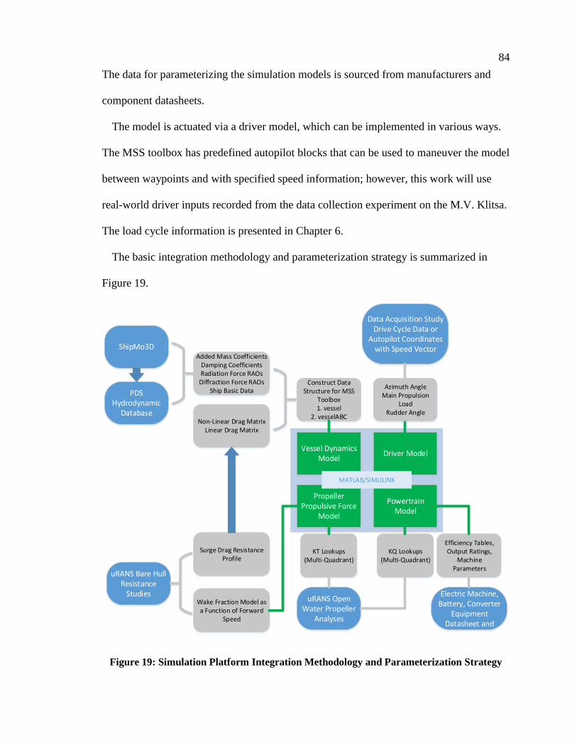
84

The data for parameterizing the simulation models is sourced from manufacturers and

component datasheets.

The model is actuated via a driver model, which can be implemented in various ways.

The MSS toolbox has predefined autopilot blocks that can be used to maneuver the model

between waypoints and with specified speed information; however, this work will use

real-world driver inputs recorded from the data collection experiment on the M.V. Klitsa.

The load cycle information is presented in Chapter 6.

The basic integration methodology and parameterization strategy is summarized in

Figure 19.

uRANS Bare Hull Resistance

Studies

Added Mass Coefficients Damping CoefficientsRadiation Force RAOsDiffraction Force RAOs

Ship Basic Data

ShipMo3D

PDS Hydrodynamic

Database

Surge Drag Resistance Profile

Non-Linear Drag MatrixLinear Drag Matrix

KT Lookups (Multi-Quadrant)

uRANS Open Water Propeller

Analyses

Propeller Propulsive Force

Model

Wake Fraction Model as a Function of Forward

Speed

KQ Lookups (Multi-Quadrant)

Powertrain Model

Prime Mover, Electric Machine,

Battery, Converter Equipment

Datasheet and Parameters

Driver Model

Efficiency Tables,Output Ratings,

Machine Parameters

Vessel Dynamics Model

Construct Data Structure for MSS

Toolbox1. vessel

2. vesselABC

Data Acquisition Study Drive Cycle Data or

Autopilot Coordinates with Speed Vector

Azimuth AngleMain Propulsion

LoadRudder Angle

MATLAB/SIMULINK

Figure 19: Simulation Platform Integration Methodology and Parameterization Strategy

85

The next chapters will develop these models in detail, illustrating the process using the

M.V. Klitsa as an example. The process of model development is intended to be

relatively parametric, and applicable to any other ship.

86

Chapter 3 Development of an Azimuthing Propeller Model for Integrated Powertrain Simulations

3.1 Model Development Methodology

Chapter 2 presented an overview of dynamic models that can be used for thrust and

torque prediction, primarily in the context of model-based control development. The

development of accurate thrust models is particularly important in high precision

applications such as dynamic position, but it also provides a method of predicting power

system loads during dynamic simulation, allowing aggregate performance to be analyzed

over different mission cycles. For the case study of the Klitsa, the task is to develop a

computationally efficient model of an azimuthing propeller, which will frequently

encounter off-design propeller conditions when traveling in-and-out of berth.

First quadrant data is generally quite easy to obtain from the propeller manufacturer;

however, acquiring data for beyond the first quadrant is often difficult. As a result, RANS

CFD has been systematically deployed to perform parameter sweeps aimed at generating

the necessary dataset to capture all realistic operating conditions. This dataset will create

2D lookup surfaces to estimate the load torque load acting on the IPS, as well as the

actuation forces for the vessel in the time-domain.

Lookup table based performance models are common practice in automotive power

system models, as they provide an excellent method of distilling down complex physics

into a computationally efficient empirical models. Over time, and as the marine industry

evolves to adopt MBD in practice, manufactures will likely begin to provide simulation

models during the initial design phase as is done in the automotive industry.

This chapter systematically develops the simulation model for the azimuthing thrusters

currently installed on the M.V. Klitsa. The work required to parameterize the equations

87

was a collaborative effort between Rahimpour and Andersen [92]. The CAD model

generation, design of CFD experiment, and implementation of CFD results into the

reduced order simulation model was conducted by the author of this work. The

configuration and execution of CFD studies was conducted by Rahimpour with some

support from Andersen. This chapter will systematically present the development process

including,

a) The propeller’s geometry generation and assumptions

b) Definition of quadrants and model layout

c) CFD results and validation

d) Simulink-based propeller model implementation

3.1.1 Thruster Geometry

The M.V. Klitsa is equipped with two well-mounted azimuthing propellers to enable a

high degree of maneuverability. These units are designed for single-direction operation,

as is typical when coupled to a diesel engine. The azimuthing tower enables thrust to be

directed in any direction within the horizontal plane, regardless of the ship’s direction of

travel.

The first quadrant propeller coefficient curves were acquired from the manufacturer to

serve as a validation tool for both the CFD analyses and the dynamic simulation model. A

3D geometry of the propeller was not provided by the manufacturer. Instead, the

geometry was created from an electronic 2D drawing illustrating the propeller blade

section geometry as function of radius. The drawing did not provide pitch distribution

explicitly; however, the preliminary design documentation provided to BC Ferries from

provided some pitch information that was leveraged to complete the 3D CAD model.

88

With the available information, the 3D geometry was approximated by tracing the 2D

blade sections in CAD using Draftsight. The section profile data points were then

imported into a 2D sketch within NX with the sketch plane tangent to a cylindrical

surface of the respective radial sections. The 2D points were aligned using the pitch

distribution data. Using the point of intersection between the directrix and the cylindrical

blade section surface as the locating datum point, the 2D profile was wrapped to the

cylindrical surface to create the blade section profile curve. This was repeated

systematically until the full set of 3D profile curves were in place, thus allowing for

surfaces to be built. The process of geometry creation is illustrated in Figure 20 through

Figure 23.

This procedure, though somewhat crude, produced a plausible geometry that provided

excellent results when compared to the manufacturer data, as will be seen section 3.3.1.1.

The thruster also contains a standard 19A duct whose geometry is presented in Carlton

[51]. The hub diameter and cone angle were approximated, and the blending of the blade

was created using a surface extension tool in NX. The geometry has been removed of all

fillets and edge breaks for import into StarCCM+ for RANS analysis.

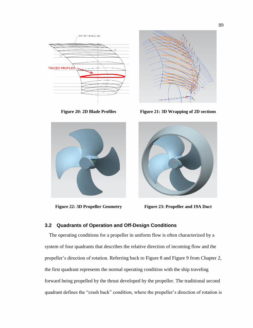
89

Figure 20: 2D Blade Profiles

Figure 21: 3D Wrapping of 2D sections

Figure 22: 3D Propeller Geometry

Figure 23: Propeller and 19A Duct

3.2 Quadrants of Operation and Off-Design Conditions

The operating conditions for a propeller in uniform flow is often characterized by a

system of four quadrants that describes the relative direction of incoming flow and the

propeller’s direction of rotation. Referring back to Figure 8 and Figure 9 from Chapter 2,

the first quadrant represents the normal operating condition with the ship traveling

forward being propelled by the thrust developed by the propeller. The traditional second

quadrant defines the “crash back” condition, where the propeller’s direction of rotation is

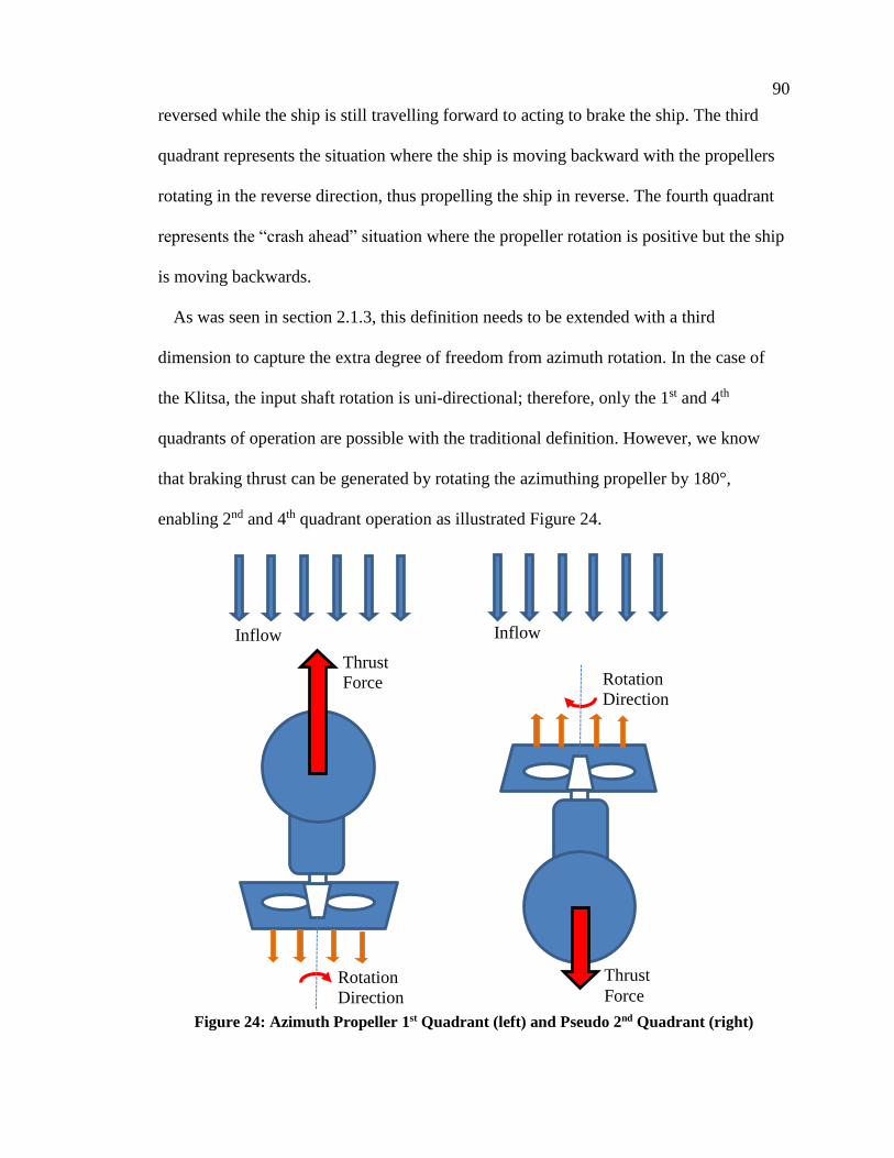
90

reversed while the ship is still travelling forward to acting to brake the ship. The third

quadrant represents the situation where the ship is moving backward with the propellers

rotating in the reverse direction, thus propelling the ship in reverse. The fourth quadrant

represents the “crash ahead” situation where the propeller rotation is positive but the ship

is moving backwards.

As was seen in section 2.1.3, this definition needs to be extended with a third

dimension to capture the extra degree of freedom from azimuth rotation. In the case of

the Klitsa, the input shaft rotation is uni-directional; therefore, only the 1st and 4th

quadrants of operation are possible with the traditional definition. However, we know

that braking thrust can be generated by rotating the azimuthing propeller by 180°,

enabling 2nd and 4th quadrant operation as illustrated Figure 24.

Figure 24: Azimuth Propeller 1st Quadrant (left) and Pseudo 2nd Quadrant (right)

Thrust

Force

Inflow

Rotation

Direction

Inflow

Thrust

Force

Rotation

Direction

91

If the propeller were able to reverse direction, this would give a 3-dimensional cube

that describes 8 possible operating conditions. In this work, the propeller’s rotation will

remain uni-directional, and the model has been created using lookup tables based on

quadrant angle β, and the relative flow angle α,

𝛽 = atan2 (𝑉𝑎

0.7𝜋𝑛𝐷) ( 3-1 )

𝛼 ≡ 𝛼𝑎𝑧𝑖 − 𝛼𝑅𝐹 ( 3-2 )

This quadrant angle definition replaces the standard advance ratio term to eliminate the

discontinuity at zero propeller speed, making it more robust for simulation. The quadrant

angle combined with incident flow angle define the relative direction of propeller thrust

relative to the ship’s motion. The relative angle of flow α is given by the angle between

incoming flow seen by the propeller and azimuth angle. An illustration of the relative

flow angle is provided in section 3.4.1 in the context of actuation forces for the true

thruster configuration. The top-level block diagram of the lookup-based model is shown

in Figure 25.

KT_Lookup(β,α)

KQ_Lookup(β,α)

β

β

α

α

KT

KQ

Figure 25: Top-level Lookup Table Block Diagram

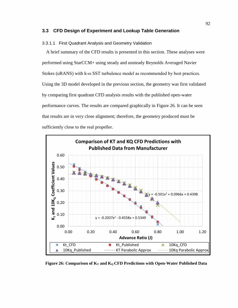
92

3.3 CFD Design of Experiment and Lookup Table Generation

3.3.1.1 First Quadrant Analysis and Geometry Validation

A brief summary of the CFD results is presented in this section. These analyses were

performed using StarCCM+ using steady and unsteady Reynolds Averaged Navier

Stokes (uRANS) with k-ω SST turbulence model as recommended by best practices.

Using the 3D model developed in the previous section, the geometry was first validated

by comparing first quadrant CFD analysis results with the published open-water

performance curves. The results are compared graphically in Figure 26. It can be seen

that results are in very close alignment; therefore, the geometry produced must be

sufficiently close to the real propeller.

Figure 26: Comparison of KT and KQ CFD Predictions with Open-Water Published Data

y = -0.2037x2 - 0.4558x + 0.5349

y = -0.501x2 + 0.0966x + 0.4398

0.00

0.10

0.20

0.30

0.40

0.50

0.60

0.00 0.20 0.40 0.60 0.80 1.00 1.20

KT

and

10

KQ

Co

effi

cien

t V

alu

es

Advance Ratio (J)

Comparison of KT and KQ CFD Predictions with Published Data from Manufacturer

Kt_CFD Kt_Published 10Kq_CFD10Kq_Published KT Parabolic Approx 10Kq Parabolic Approx

93

Both the thrust coefficients and torque coefficients show excellent agreement. Note that

the torque coefficient has been scaled by a factor of 10 for clarity, as is customary. A

parabolic approximation trendline has been fit to both KT and KQ results. The application

of a parabolic approximation is an agreement with the results presented by Kim and

Chung [60]. An image of the 1st quadrant solution produced by StarCCM+ is provided in

Figure 27. This plot illustrates the velocity magnitude for a cross-sectional plane through

the domain. The velocity profile is intuitive and flow field is physical.

The advance ratio for CFD parameter sweeps is bounded by the ratings of the propeller

and the maximum ship speed. The maximum attainable speed for the hull is

approximately 10 knots. The propeller’s maximum operating speed is 464rpm, and the

minimum is set by the engine idle speed of approximately 650rpm. This implies that the

maximum realizable advance ratio can be calculated by,

𝐽𝑚𝑎𝑥 =𝑉𝑎𝑛𝐷

=(10𝑘𝑛𝑜𝑡𝑠)

0.5144 𝑚/𝑠𝑘𝑛𝑜𝑡

(650/3.882𝑟𝑝𝑚60𝑠/𝑚𝑖𝑛

) 1.135𝑚≈ 1.6 ( 3-3)

If the results from the Figure 26 are extrapolated, it can be seen that the thrust and

torque coefficient will actually become negative at an advance ratio of 1.6. This implies

that the propeller will become overdriven and will act similar to a turbine. The thrust

force would transform into an additional resistive drag force, and mechanical power will

be added to the powertrain system rather than being consumed. The overdriven situation

is a short-term transient, and will last only momentarily when engines are initially

ramped back after traveling at full speed. Operators are aware of this phenomenon and

generally reduce engines gradually. For the purposes of this study, the propeller model

will be limited in the first quadrant to positive values of thrust and torque coefficients.

94

Figure 27: CFD Image Showing Velocity Magnitude Profile in 1st Quadrant

3.3.1.2 Anti-Directional and Vague-Directional Operation

The first quadrant CFD results agreed very well with published data; however, data

was not available for the propeller at non-incident inflow conditions. As will be seen in

Chapter 6, the ferry often uses a full 180° rotation of the thrust for braking while

approaching berth; therefore, the CFD experiment sought to provide a complete set of

data with sufficient resolution to properly model the opposing directional state. In the

work of Kim and Chung [60], the authors experimentally studied the steady state thrust

and torque production of an ROV thruster in the first quadrant, as well as in the opposing

directional pseudo-second quadrant. The term pseudo-second quadrant has been coined in

this work to differentiate between the reversal of the propeller’s direction, as is defined in

traditional literature, with the effect of rotating of a propeller by 180° with an azimuthing

mechanism. Note that if the propeller is symmetric and no duct is present, the

performance would be approximately equivalent for true second quadrant, and pseudo-

second quadrant conditions.

Kim and Chung [60] observed that this pseudo-second quadrant operating regime

exhibited two distinctly different flow fields separated by an inflection point termed the

Critical Advance Ratio (CAR). This was also observed in the CFD results as is shown in

Figure 28 through Figure 31.

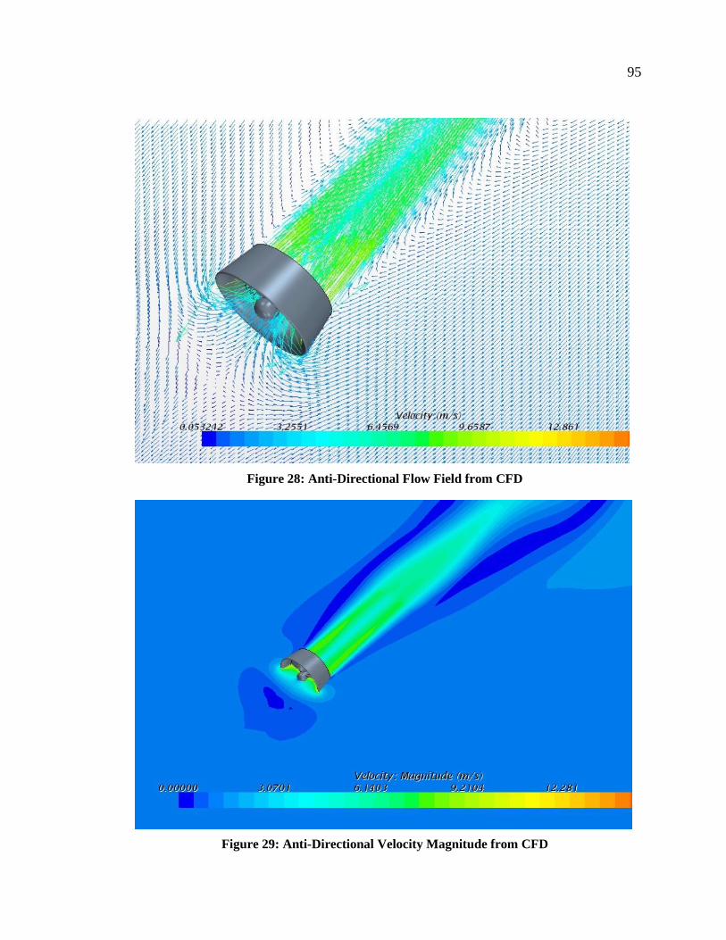
95

Figure 28: Anti-Directional Flow Field from CFD

Figure 29: Anti-Directional Velocity Magnitude from CFD

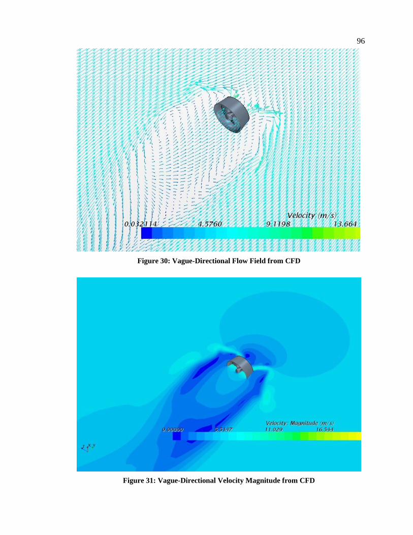
96

Figure 30: Vague-Directional Flow Field from CFD

Figure 31: Vague-Directional Velocity Magnitude from CFD

97

Kim and Chung describes the these two flow patterns as,

a) Anti-directional

b) Vague-directional

The anti-directional state represents the situation where the propeller delivers sufficient

momentum to the flow to effectively counter the momentum of the incoming freestream

fluid. A contracting thrust tube develops upstream, in the direction opposing flow, as can

be seen in Figure 28 and Figure 29. This situation occurs when the rotational speed of the

propeller is relatively high in comparison to the flow velocity, or at small advance ratios.

The vague-directional state occurs when the incoming freestream velocity momentum

dominates, and the propeller cannot impart sufficient momentum to overcome the

incoming flow. With sufficient incoming freestream velocity, the flow through the

propeller will actually reverse. Interestingly, this situation produces an increase in thrust

force. This is not entirely unexpected when we recognize that the maximum thrust of a

propeller is produced in the bollard pull condition; therefore, if the net force balance

between thrust production and inflow momentum produces close to net zero velocity

inlet, then the propeller may be acting in a state similar to bollard pull.

There is a point where the vague directional relationship will ultimately breakdown,

but this occurs outside the physical operating conditions of this application. For example,

extensive tests have been conducted at MARIN using standard series propellers to plot

complete sets of four quadrant data, see Carlton [51]. The vague-directional state is

shown in Figure 30 and Figure 31.

98

The results from the CFD studies performed by Rahimpour and Andersen [92] on the

thruster in opposing flow conditions are illustrated in Figure 32. An inflection point is

observed at an advance ratio around -0.3, which is consistent with the CAR seen by Kim

and Chung [60]. A parabolic trendline fit also illustrates that thrust prediction models

based on parabolic approximations provide a reasonable approximation for both flow

regimes.

Figure 32: Thrust and Torque Coefficient for Pseudo-Second Quadrant Results from CFD

No clear inflection point was observed for the torque coefficient, which remained

somewhat flat in the anti-directional regime, then increased in the vague-directional

regime. To further validate the CFD process, a similar experiment was conducted on the

well the Kaplan Ka4-70 propeller with 19A duct whose complete set of four quadrant

data is published in Carlton [51]. The results for pseudo 2nd quadrant, or opposing flow

conditions, matched the published data thereby validating the CFD analysis procedure

and analysis configuration.

y = -6.9703x2 - 1.8073x + 0.4956

y = 0.302x2 - 0.0857x + 0.3537

0.000

0.100

0.200

0.300

0.400

0.500

0.600

0.700

0.800

0.900

1.000

-0.90 -0.80 -0.70 -0.60 -0.50 -0.40 -0.30 -0.20 -0.10 0.00

KT

10KQ

Advance Ratio J

Thrust and Torque Coefficients for Pseudo-Second Quadrant Result from CFD

KT Anti-Directional KT Vague-Directional KQ Anti-Directional

KQ Vague-Directional AD Parabolic Fit VD Parabolic Fit

Anti-directionalVague-directional

99

3.3.1.3 Oblique Flow and Angled Operation of Azimuthing Thrusters

The final portion of the CFD experiment involved an investigation of non-incident or

oblique flow over the propeller. The azimuthing thrusters on the Klitsa allow for thrust to

be directed in any direction within the horizontal plane, regardless of the vessel’s travel

direction. During maneuvers in-and-out of berth, the relative angle between the

propeller’s inflow field and its azimuth orientation will regularly be non-zero. This non-

incident flow condition will impact both thrust production, as well as powertrain loading.

When approaching berth, the operator will rotate the propellers to 180° in preparation for

braking. They will also tailor the direction of rotation to utilize the transient thrust

production to direct the bow or stern as desired.

Due to the large transient forces associated with rotation of the propeller, this process is

generally performed at reduced ship speed and at low propeller speed to minimize the

mechanical stress. A sharp torsional transient occurs on the powertrain system when

these rotations are performed. By analyzing the operational data collected on the Klitsa,

we can define a series of CFD analyses aimed at quantifying the impact of oblique flow

on thrust and torque production at different relative flow angles under real operating

conditions.

Based on observation of the data, the propeller rotation is typically performed just

above the engine’s idle speed so to maintain clutch engagement, yet not overload the

engine with the torque transient. Consequently, the design of experiment was limited to

the single propeller speed, but with six different forward speed operating points to

provide reasonable resolution. For each of these six operating conditions, CFD analyses

were conducted to produce the propeller’s thrust and torque coefficients by sweeping the

incident flow angle in increments of 30°.

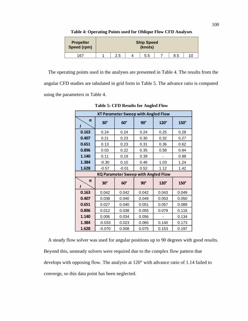
100

Table 4: Operating Points used for Oblique Flow CFD Analyses

Propeller Speed (rpm)

Ship Speed (knots)

167 1 2.5 4 5.5 7 8.5 10

The operating points used in the analyses are presented in Table 4. The results from the

angular CFD studies are tabulated in grid form in Table 5. The advance ratio is computed

using the parameters in Table 4.

Table 5: CFD Results for Angled Flow

A steady flow solver was used for angular positions up to 90 degrees with good results.

Beyond this, unsteady solvers were required due to the complex flow pattern that

develops with opposing flow. The analysis at 120° with advance ratio of 1.14 failed to

converge, so this data point has been neglected.

α

J

0.24 0.24 0.24 0.25 0.28

0.21 0.23 0.30 0.32 0.27

0.13 0.23 0.31 0.36 0.62

0.03 0.22 0.35 0.58 0.84

0.11 0.19 0.39 - 0.98

-0.30 0.10 0.46 1.03 1.24

-0.57 -0.01 0.52 1.12 1.42

α

J

0.042 0.042 0.042 0.043 0.049

0.038 0.040 0.049 0.053 0.050

0.027 0.040 0.051 0.057 0.089

0.012 0.038 0.055 0.079 0.116

0.006 0.034 0.056 - 0.134

-0.033 0.023 0.065 0.140 0.173

-0.070 0.008 0.075 0.153 0.1971.628

0.163

0.407

0.651

0.896

1.140

1.384

1.628

KQ Parameter Sweep with Angled Flow

30° 60° 90° 120° 150°

0.163

0.407

0.651

0.896

1.140

1.384

KT Parameter Sweep with Angled Flow

30° 60° 90° 120° 150°

101

3.4 Development of Simulink-Based Thrust Model and Validation

The CFD analyses established a dataset for the spectrum of potential operating points

that the propeller will encounter in real-world operation. This data represents quasi-

steady state thrust and torque characteristics of the propeller. The objective now is

compile this data to generate a lookup surface that can be implemented into the

simulation model. In the case of the Klitsa, it is convenient to lump the right-angle

gearbox and driveline into the azimuthing propeller model. Both thrust and torque

coefficients are computed using “2D Lookup Table” Simulink block with advance angle

β, and relative flow angle α as signal inputs. The output is then scaled based on Equations

( 2-17 ) and ( 2-18 ) and to produce the dimensionalized values.

The mechanical drivetrain system was originally implemented using Simscape to

provide a more physical representation of the system; however, it was found that

simulation times increased drastically with this approach and the model was reverted

back to a basic Simulink model. The magnitude of the thrust force produced by the

propeller is decomposed into directional components to build the thrust force actuation

vector 𝝉𝑝𝑟𝑜𝑝, expressed in body-fixed coordinates. The top level layout of the model is

presented in Figure 33.

Because the ramp rate of the propellers is relatively low due to the large forces and

inertias at play, the dynamics of thrust production from the fluid momentum equation

were assumed to be negligible; therefore, quasi steady-state data has been assumed. As

will be seen in Chapter 7, this approximation produces satisfactory results for extracting

powertrain loads. Future work should investigate the dynamic effects of thrust

development to verify this assumption.

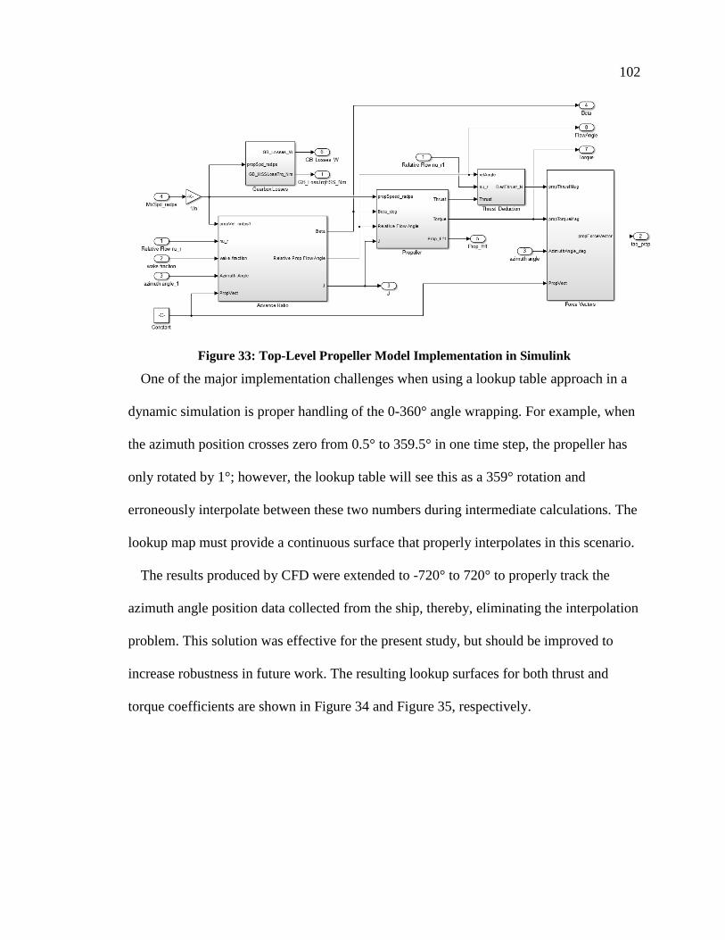
102

Figure 33: Top-Level Propeller Model Implementation in Simulink

One of the major implementation challenges when using a lookup table approach in a

dynamic simulation is proper handling of the 0-360° angle wrapping. For example, when

the azimuth position crosses zero from 0.5° to 359.5° in one time step, the propeller has

only rotated by 1°; however, the lookup table will see this as a 359° rotation and

erroneously interpolate between these two numbers during intermediate calculations. The

lookup map must provide a continuous surface that properly interpolates in this scenario.

The results produced by CFD were extended to -720° to 720° to properly track the

azimuth angle position data collected from the ship, thereby, eliminating the interpolation

problem. This solution was effective for the present study, but should be improved to

increase robustness in future work. The resulting lookup surfaces for both thrust and

torque coefficients are shown in Figure 34 and Figure 35, respectively.

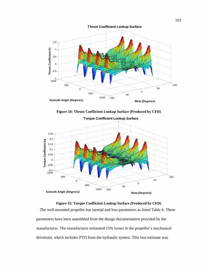
103

Figure 34: Thrust Coefficient Lookup Surface (Produced by CFD)

Figure 35: Torque Coefficient Lookup Surface (Produced by CFD)

The well-mounted propeller has inertial and loss parameters as listed Table 6. These

parameters have been assembled from the design documentation provided by the

manufacturer. The manufacturer estimated 15% losses in the propeller’s mechanical

drivetrain, which includes PTO from the hydraulic system. This loss estimate was

-100

-50

0

50

100

-1000

-500

0

500

1000-1

-0.5

0

0.5

1

1.5

Beta (Degrees)

Thrust Coefficient Lookup Surface

Azimuth Angle (Degrees)

Th

rust

Co

eff

icie

nt

Kt

-100

-50

0

50

100

-1000

-500

0

500

1000-0.1

-0.05

0

0.05

0.1

0.15

0.2

0.25

Beta (Degrees)

Torque Coefficient Lookup Surface

Azimuth Angle (Degrees)

To

rqu

e C

oeff

icie

nt

Kq

104

assumed to be at maximum rated power output and rated speed. A linear torsional

damping term was implemented to account for dynamic losses, with the damping

coefficient calculated to produce 15% power loss at rated conditions. The resulting

resistive torque was implemented on the high speed side of the gearbox to be included in

the electric drive’s rotational equation of motion.

Table 6: Summary of Propeller System Model Parameters

PROPELLER PROPERTIES VALUE UNIT

PROPELLER ROTATIONAL INERTIA 11.6 kg-m2

PROPELLER GB REDUCTION 3.882

GB/SHAFT LOSSES 0.85

TORQUE DAMPING COEFFICIENT (LSS) 16.6 Nm/rad/s

PROPELLER DENSITY 7650 kg/m3

3.4.1 Thruster Configuration and Vessel Actuation Forces for M.V. Klitsa

The M.V. Klitsa’s thruster configuration differs from most conventional vessels in that

the units are not symmetric about the ship’s longitudinal centreline. Because the ferry is

double-ended, a single thruster has been placed on opposite ends of the ship to enable a

high degree of maneuverability. The thrust production from each thruster will not be

equal as a result of the wake fraction effect. The thruster configuration is illustrated in

Figure 36.

Figure 36: Thruster Configuration on the M.V. Klitsa

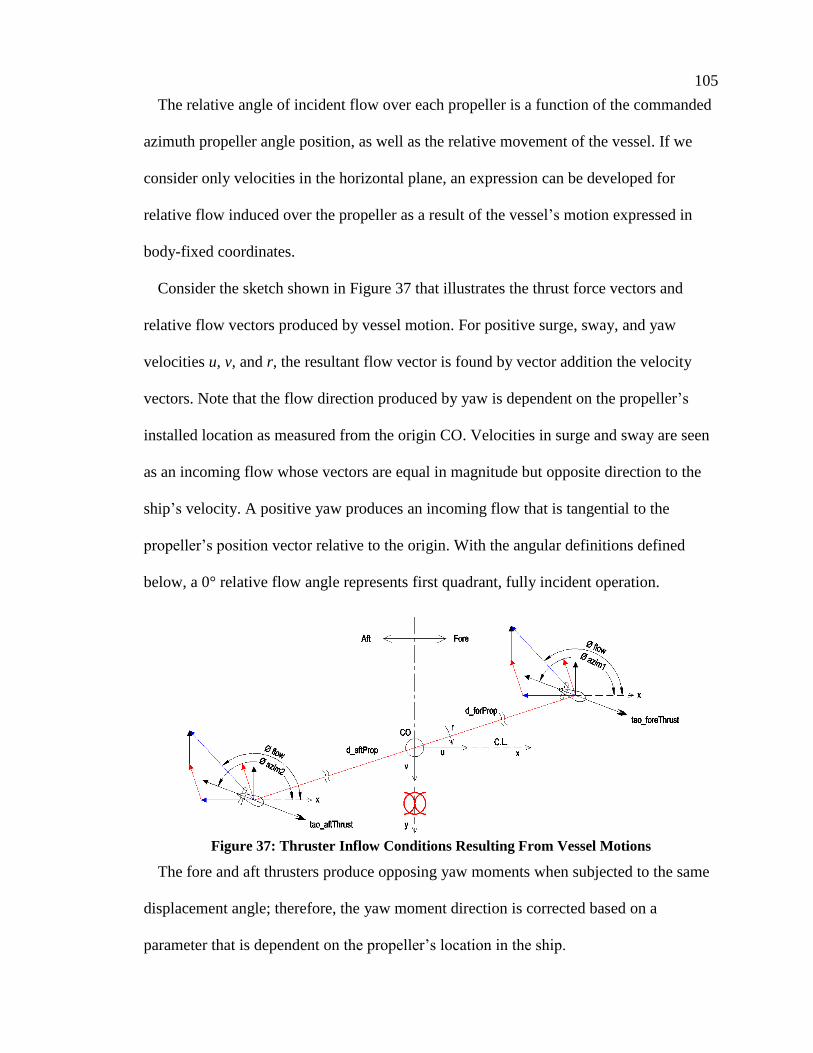
105

The relative angle of incident flow over each propeller is a function of the commanded

azimuth propeller angle position, as well as the relative movement of the vessel. If we

consider only velocities in the horizontal plane, an expression can be developed for

relative flow induced over the propeller as a result of the vessel’s motion expressed in

body-fixed coordinates.

Consider the sketch shown in Figure 37 that illustrates the thrust force vectors and

relative flow vectors produced by vessel motion. For positive surge, sway, and yaw

velocities u, v, and r, the resultant flow vector is found by vector addition the velocity

vectors. Note that the flow direction produced by yaw is dependent on the propeller’s

installed location as measured from the origin CO. Velocities in surge and sway are seen

as an incoming flow whose vectors are equal in magnitude but opposite direction to the

ship’s velocity. A positive yaw produces an incoming flow that is tangential to the

propeller’s position vector relative to the origin. With the angular definitions defined

below, a 0° relative flow angle represents first quadrant, fully incident operation.

Figure 37: Thruster Inflow Conditions Resulting From Vessel Motions

The fore and aft thrusters produce opposing yaw moments when subjected to the same

displacement angle; therefore, the yaw moment direction is corrected based on a

parameter that is dependent on the propeller’s location in the ship.

106

Chapter 4 Development of a Time-Domain Dynamics Model for a

Barge-Type Ferry Hull

4.1 Development of Ship Inertial Model

The M.V. Klitsa was constructed in 1952 with the original drawings completed by

hand. Though 2D CAD drawings were available from BC Ferries illustrating the

structural plans, the primary source of information for the ship’s buoyancy and trim

properties is given in the ship’s trim and stability book [93]. This document provides

hydrostatic stability information along with estimates for the ship’s centre of gravity

(CG) and buoyancy centre for different operating conditions. Though the stability book

offers insight into hydrostatic properties, it does not offer much insight into the inertial

properties beyond vessel mass.

An accurate approximation of the ship’s inertial properties is imperative to achieving

good modeling results for vessel motion. To estimate the moments of inertia governing

the roll-pitch-yaw subsystem, a simplified 3D CAD representation was created to

estimate mass properties numerically. The 3D hull representation is also required for

import into ShipMo3D for computation of hydrodynamic coefficients. Using the

information contained within the stability book, the 3D CAD was systematically detailed

to achieve the vessel mass and CG positions published in the document.

Two excerpt from the blueprints showing the primary structural layout of the hull are

illustrated in Figure 38 and Figure 39. Using these drawings, the hull sections were

modeled systematically in CAD to produce a realistic mass distribution for the steel

structure. Most of the girder, plate, and flange dimensions and material thicknesses were

provided on the drawing. Anything not labeled was assumed to be ¼” thick mild steel

plate.

107

Figure 38: Cross-Sectional View Illustrating Transverse Support Structure

Figure 39: Crossing Sectional View Illustrating Longitudinal Support Structure

The mass of the hull structure alone was computed by the CAD software to be 270

tonnes. The lightship displacement of the Klitsa, according to the stability book, is given

to be 334.5 tonnes leaving around 64 tonnes unaccounted for.

The next step was to estimate the dead weight of the permanent equipment and fixtures

onboard. Approximations for the main equipment were estimated from datasheets, and

information found on similar products. The decks also include auxiliary equipment, tools,

fixtures, safety systems, and additional structural elements. Modeling of all individual

components is clearly unfeasible; therefore, the passenger and crew areas were intuitively

separated into different regions where a uniform distributed load could be applied. This

approach is similar to that applied in building construction. For this inertial model, the

normal human occupied spaces were broken out as follows:

108

a) Office/Kitchen Space

b) Industrial Space

c) Passenger Space

The assumed values for distributed uniform loads for each section have been taken

from building code to approximate the additional mass for onboard equipment to

reconcile the lightship discrepancy. A static block of mass was created for each of these

regions to represent the assumed distributed load, and placed 0.5m above the floor to

approximate the height of the centre of gravity.

The “Normal Departure” condition was selected from the stability book as the primary

means of comparison and validation. Normal departure implies that all fuel, oil, and lube

tanks are topped up before departure. The fresh water tanks are full, but sewage tanks are

empty. These additional fluid masses were accounted for using the specific gravity of

each fluid listed in [94] and placing a mass at the volumetric centre of each tank.

Table 7 shows a summary of the stability book hydrostatic parameters and assumed

vessel loading for the ship model. This table also compares the CG location predicted by

the CAD model versus that published in the stability book. Note that the datum for

measurements of the longitudinal centre of gravity (LCG), transverse centre of gravity

(TCG), and vertical centre of gravity (VCG) is located on the baseline at midships, an the

longitudinal centreline of the ship.

The CG location prediction of the CAD model is in good agreement with that of the

stability book, and the mass distribution should produce a good estimate for the inertial

properties.

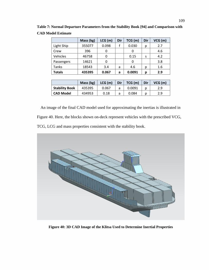
109

Table 7: Normal Departure Parameters from the Stability Book [94] and Comparison with

CAD Model Estimate

Mass (kg) LCG (m) Dir TCG (m) Dir VCG (m)

Light Ship 355077 0.098 f 0.030 p 2.7

Crew 396 0 0 4.6

Vehicles 46758 0 0.15 s 4.2

Passengers 14621 0 0 3.8

Tanks 18543 3.4 a 4.6 p 1.6

Totals 435395 0.067 a 0.0091 p 2.9

Mass (kg) LCG (m) Dir TCG (m) Dir VCG (m)

Stability Book 435395 0.067 a 0.0091 p 2.9

CAD Model 434953 0.18 a 0.084 p 2.9

An image of the final CAD model used for approximating the inertias is illustrated in

Figure 40. Here, the blocks shown on-deck represent vehicles with the prescribed VCG,

TCG, LCG and mass properties consistent with the stability book.

Figure 40: 3D CAD Image of the Klitsa Used to Determine Inertial Properties

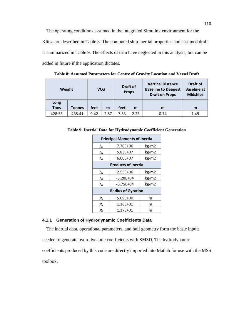
110

The operating conditions assumed in the integrated Simulink environment for the

Klitsa are described in Table 8. The computed ship inertial properties and assumed draft

is summarized in Table 9. The effects of trim have neglected in this analysis, but can be

added in future if the application dictates.

Table 8: Assumed Parameters for Centre of Gravity Location and Vessel Draft

Weight VCG Draft of Props

Vertical Distance Baseline to Deepest

Draft on Props

Draft of Baseline at Midships

Long Tons Tonnes feet m feet m m m

428.53 435.41 9.42 2.87 7.33 2.23 0.74 1.49

Table 9: Inertial Data for Hydrodynamic Coefficient Generation

Principal Moments of Inertia

Ixx 7.70E+06 kg-m2

Ixy 5.83E+07 kg-m2

Ixz 6.00E+07 kg-m2

Products of Inertia

Ixy 2.55E+06 kg-m2

Iyz -3.28E+04 kg-m2

Ixz -5.75E+04 kg-m2

Radius of Gyration

Rx 5.09E+00 m

Ry 1.16E+01 m

Rz 1.17E+01 m

4.1.1 Generation of Hydrodynamic Coefficients Data

The inertial data, operational parameters, and hull geometry form the basic inputs

needed to generate hydrodynamic coefficients with SM3D. The hydrodynamic

coefficients produced by this code are directly imported into Matlab for use with the MSS

toolbox.

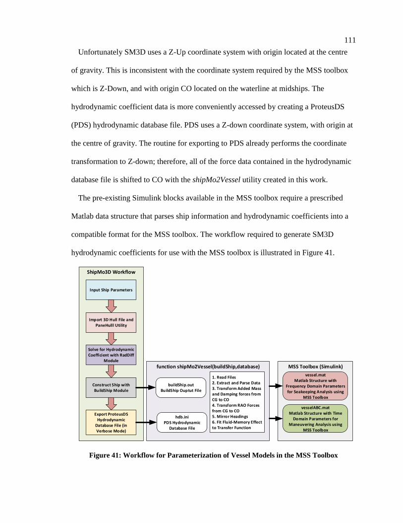
111

Unfortunately SM3D uses a Z-Up coordinate system with origin located at the centre

of gravity. This is inconsistent with the coordinate system required by the MSS toolbox

which is Z-Down, and with origin CO located on the waterline at midships. The

hydrodynamic coefficient data is more conveniently accessed by creating a ProteusDS

(PDS) hydrodynamic database file. PDS uses a Z-down coordinate system, with origin at

the centre of gravity. The routine for exporting to PDS already performs the coordinate

transformation to Z-down; therefore, all of the force data contained in the hydrodynamic

database file is shifted to CO with the shipMo2Vessel utility created in this work.

The pre-existing Simulink blocks available in the MSS toolbox require a prescribed

Matlab data structure that parses ship information and hydrodynamic coefficients into a

compatible format for the MSS toolbox. The workflow required to generate SM3D

hydrodynamic coefficients for use with the MSS toolbox is illustrated in Figure 41.

MSS Toolbox (Simulink)function shipMo2Vessel(buildShip,database)

ShipMo3D Workflow

Input Ship Parameters

Import 3D Hull File and PaneHulll Utility

Solve for Hydrodynamic Coefficient with RadDiff

Module

Export ProteusDS Hydrodynamic

Database File (in Verbose Mode)

Construct Ship with BuildShip Module

buildShip.outBuildShip Ouptut File

hdb.iniPDS Hydrodynamic

Database File

1. Read Files2. Extract and Parse Data3. Transform Added Mass and Damping forces from CG to CO4. Transform RAO Forces from CG to CO5. Mirror Headings6. Fit Fluid-Memory Effect to Transfer Function

vessel.matMatlab Structure with

Frequency Domain Parameters for Seakeeping Analysis using

MSS Toolbox

vesselABC.matMatlab Structure with Time

Domain Parameters for Maneuvering Analysis using

MSS Toolbox

Figure 41: Workflow for Parameterization of Vessel Models in the MSS Toolbox

112

SM3D offers a simple graphical user interface for configuring the hydrodynamic

analysis, and provides a 3D geometry import tool to facilitate construction of the hull

geometry. The panelled hull used for the analysis is shown in Figure 42.

Figure 42: Panelled Hull in ShipMo3D

The computed added mass and damping coefficients are presented in Figure 43. The

results are fairly well behaved, although some oscillations and ripple are present in the

plots indicating some numerical inconsistencies. As expected, the damping coefficients

trend to zero as the frequency increases; however, these results only illustrate the

diagonal elements of the added mass and damping force matrices. It will be seen in

section 4.1.4.1 that SM3D produced numerical errors when computing off-diagonal

coefficients.

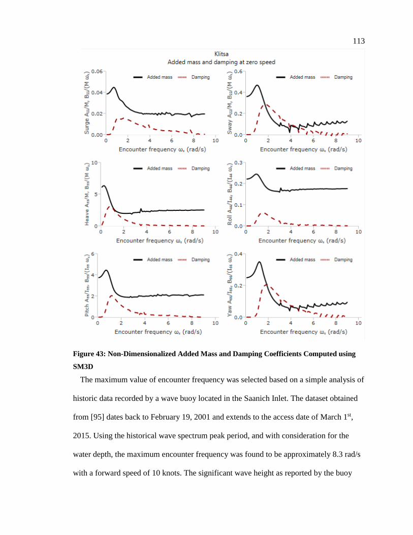
113

Figure 43: Non-Dimensionalized Added Mass and Damping Coefficients Computed using

SM3D

The maximum value of encounter frequency was selected based on a simple analysis of

historic data recorded by a wave buoy located in the Saanich Inlet. The dataset obtained

from [95] dates back to February 19, 2001 and extends to the access date of March 1st,

2015. Using the historical wave spectrum peak period, and with consideration for the

water depth, the maximum encounter frequency was found to be approximately 8.3 rad/s

with a forward speed of 10 knots. The significant wave height as reported by the buoy

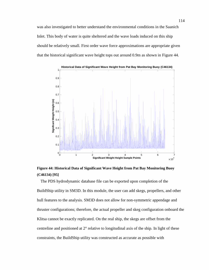
114

was also investigated to better understand the environmental conditions in the Saanich

Inlet. This body of water is quite sheltered and the wave loads induced on this ship

should be relatively small. First order wave force approximations are appropriate given

that the historical significant wave height tops out around 0.9m as shown in Figure 44.

Figure 44: Historical Data of Significant Wave Height from Pat Bay Monitoring Buoy

(C46134) [95]

The PDS hydrodynamic database file can be exported upon completion of the

BuildShip utility in SM3D. In this module, the user can add skegs, propellers, and other

hull features to the analysis. SM3D does not allow for non-symmetric appendage and

thruster configurations; therefore, the actual propeller and skeg configuration onboard the

Klitsa cannot be exactly replicated. On the real ship, the skegs are offset from the

centreline and positioned at 2° relative to longitudinal axis of the ship. In light of these

constraints, the BuildShip utility was constructed as accurate as possible with

0 1 2 3 4 5 6 7

x 104

0

0.1

0.2

0.3

0.4

0.5

0.6

0.7

0.8

0.9

1Historical Data of Significant Wave Height from Pat Bay Monitoring Buoy (C46134)

Significant Weight Height Sample Points

Sig

nif

ca

nt

We

igh

t H

eig

ht

(m)

115

longitudinally parallel skegs along the centreline, and propellers symmetrically

distributed at midships. The final representation of the wetted hull is shown in Figure 45.

Figure 45: Final BuildShip Configuration for Computing Ship Hydrodynamic Coefficients

4.1.2 Vessel Dynamics Model

The MSS toolbox contains a pre-configured block which implemented the unified

maneuvering/seakeeping Newton-Euler vessel equations of motion described in Chapter

2. This is a linearized model based about an equilibrium transit speed, which can be used

directly for this study. The linearizing approximation works quite well while the ship is in

transit and not making significant course changes. Yaw rate will be relatively small, and

the Klitsa’s barge-like hull is stable and does not typically yield much roll and pitch

action in Saanich Inlet crossing. The unified seakeeping/maneuvering equation of motion

developed with Chapter 2 with expansion of external forces is given by,

116

(𝑴𝑹𝑩 + 𝑨∞)𝒓 + (𝑪𝑹𝑩∗ + 𝑪𝑨

∗ )𝝂𝒓 +𝑫𝑳𝝂𝒓 +𝑫𝑵(𝝂𝒓)

+ ∫ 𝑲(𝑡 − 𝜏)[𝝂 − 𝑈𝒆1]𝑑𝜏𝑡

0⏟ 𝝁

+ 𝑮𝜼

= 𝝉𝑤𝑎𝑣𝑒 + 𝝉𝑤𝑖𝑛𝑑 + 𝝉𝑓𝑜𝑟𝑒𝑆𝑘𝑒𝑔 + 𝝉𝑎𝑓𝑡𝑆𝑘𝑒𝑔 + 𝝉𝑝𝑟𝑜𝑝

( 4-1 )

In this equation, the external forces acting on the body have been separated based on

the configuration of the Klitsa. Recall that this equation is represented in body fixed

coordinates, and the transformation matrix 𝑱𝚯 in Equation ( 2-84 ) will convert to inertial

coordinates. The implementation of this matrix equation in the MSS toolbox is shown in

Figure 46. The model also includes the 3-DOF non-linear maneuvering model for the

surge-sway-yaw subsystems and allows for a linear viscous matrix 𝑫𝑳 to be specified.

The hydrodynamic coefficients from SM3D produce the added mass and potential

damping data for the matrix equation above. Now, the viscous and non-linear drag

matrices need to be systematically developed using CFD and empirical data coefficients

to fully define damping matrix 𝑫. Lastly, the fluid memory effects need to be

incorporated into the equation using the state space approximation technique described in

section 2.3.6.

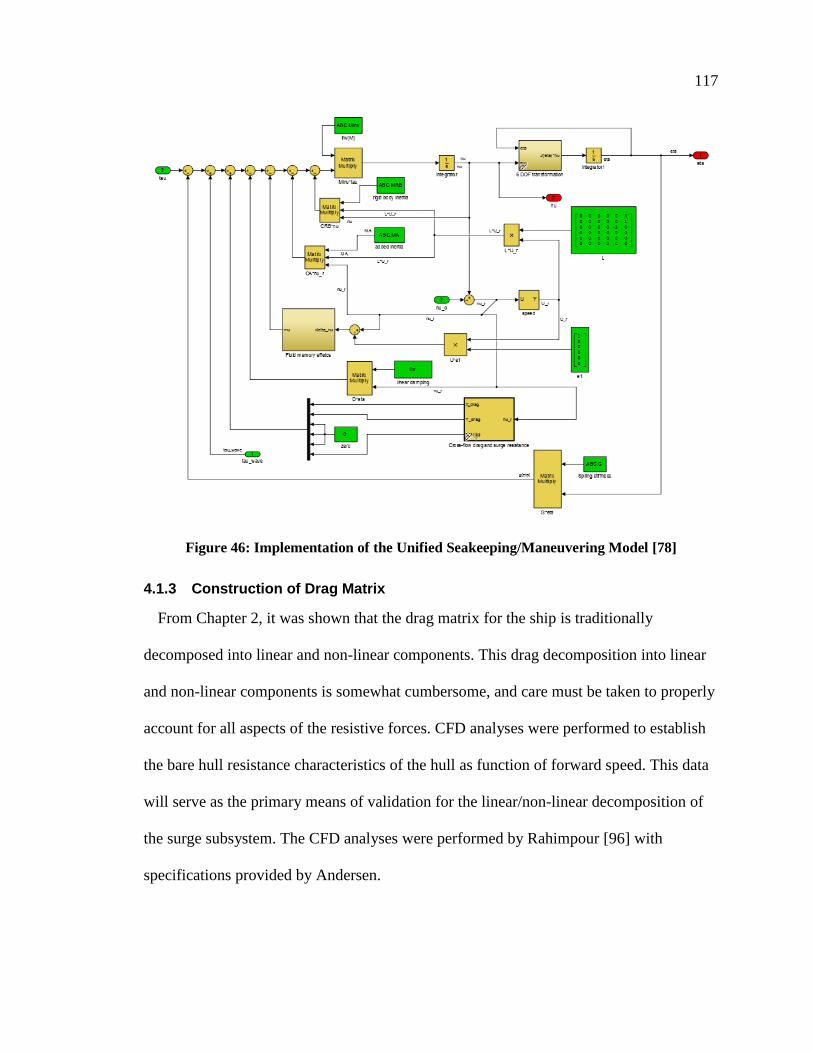
117

Figure 46: Implementation of the Unified Seakeeping/Maneuvering Model [78]

4.1.3 Construction of Drag Matrix

From Chapter 2, it was shown that the drag matrix for the ship is traditionally

decomposed into linear and non-linear components. This drag decomposition into linear

and non-linear components is somewhat cumbersome, and care must be taken to properly

account for all aspects of the resistive forces. CFD analyses were performed to establish

the bare hull resistance characteristics of the hull as function of forward speed. This data

will serve as the primary means of validation for the linear/non-linear decomposition of

the surge subsystem. The CFD analyses were performed by Rahimpour [96] with

specifications provided by Andersen.

118

The CFD data set for total hull resistance, as function of vessel forward speed, is

presented in Figure 47. From Chapter 2, recall that the surge damping force can be

considered decoupled from the remaining degrees of freedom; therefore, the total drag

force can be written as,

𝐹𝑑𝑟𝑎𝑔 = 𝑋𝑢𝑢𝑟⏟𝐿𝑖𝑛𝑒𝑎𝑟𝐹𝑜𝑟𝑐𝑒

+1

2𝜌𝑆𝐶𝑇

∗(𝑢𝑟)|𝑢𝑟|𝑢𝑟⏟ 𝑁𝑜𝑛−𝐿𝑖𝑛𝑒𝑎𝑟

𝐹𝑜𝑟𝑐𝑒

( 4-2 )

The hull form factor was computed in accordance with ITTC1978, whereby, this

parameter was computed using the CFD results with low ship speed, i.e. where Froude

number is small. This was done in Rahimpour [96]. The frictional coefficient is computed

using equation ( 2-125 ). The term 𝐶𝑇(𝑢𝑟𝑚𝑎𝑥) is taken directly from the CFD results at

maximum speed of ten knots.

The parameters α, 𝐶𝐷, and 𝑋𝑢 can be fit to the CFD data points using the lsqcurvefit

function in Matlab to produce the best parameterization for the linear/non-linear

decomposition. The fitted results are also illustrated below in Figure 47.

There is a small discrepancy in the treatment of the hull form factor presented in

Fossen [63] and the ITTC78 guidelines. In order to explore this discrepancy, two

parameter fitting optimization routines were executed, one allowing the parameter k to be

manipulated, and the other that fixed at this value produced by ITTC78 recommendations

as performed in Rahimpour [96]. Both results are illustrated in the plot. The more

accurate model drag model is achieved by allowing modification to the hull form factor k.

The final parameters produced from both optimization routines are shown in Table 10.

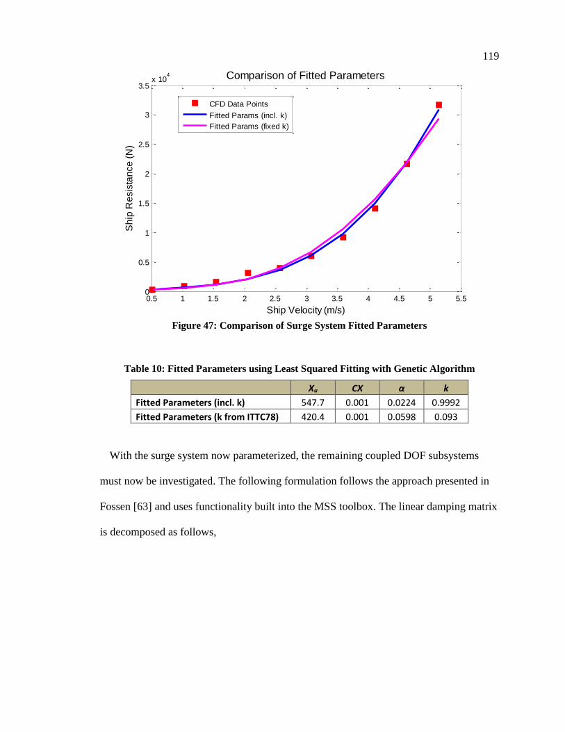
119

Figure 47: Comparison of Surge System Fitted Parameters

Table 10: Fitted Parameters using Least Squared Fitting with Genetic Algorithm

Xu CX α k

Fitted Parameters (incl. k) 547.7 0.001 0.0224 0.9992

Fitted Parameters (k from ITTC78) 420.4 0.001 0.0598 0.093

With the surge system now parameterized, the remaining coupled DOF subsystems

must now be investigated. The following formulation follows the approach presented in

Fossen [63] and uses functionality built into the MSS toolbox. The linear damping matrix

is decomposed as follows,

0.5 1 1.5 2 2.5 3 3.5 4 4.5 5 5.50

0.5

1

1.5

2

2.5

3

3.5x 10

4

Ship Velocity (m/s)

Sh

ip R

esis

tan

ce

(N

)

Comparison of Fitted Parameters

CFD Data Points

Fitted Params (incl. k)

Fitted Params (fixed k)

120

𝑫𝑳 =

[ 0 0 0 0 0 00 0 0 0 0 00 0 𝐵33(𝜔𝑛,ℎ𝑒𝑎𝑣𝑒) 0 0 0

0 0 0 𝐵44(𝜔𝑛,𝑟𝑜𝑙𝑙) 0 0

0 0 0 0 𝐵55(𝜔𝑛,𝑝𝑖𝑡𝑐ℎ) 0

0 0 0 0 0 0]

+

[ 𝑋𝑢 0 0 0 0 00 𝐵22𝑣 0 0 0 00 0 𝐵33𝑣 0 0 00 0 0 𝐵44𝑣 0 00 0 0 0 𝐵55𝑣 00 0 0 0 0 𝐵66𝑣]

( 4-3 )

The potential damping is only considered significant in heave, roll, and pitch. By

formulating a set of spring-mass-damper equations for the diagonal entries of 𝑫𝑷, the

natural frequency of each subsystem can be found numerically using the added mass and

damping coefficients computed by ShipMo3D. The MSS toolbox contains an iterative

numerical solver function natfrequencies that returns the natural frequency of the spring-

mass-damper system from hydrodynamic data. The potential damping coefficient at the

natural frequency is selected as the entry into the potential damping matrix. The reader is

directed to Fossen [63] for further details.

Selection of the linear viscous terms is a bit more ambiguous, but these terms can

provide a good means of tuning the model if accurate response data is available. Fossen

[63] offers a derivation for the linear viscous terms using the closed loop response of a

vessel under PD control. There appears to be errors in the Fossen’s equation derivation.

Furthermore, the author’s formulae use zero frequency added mass coefficients which

aren’t physical. Instead, these equations will use the infinite frequency values and viscous

damping terms are estimated by,

121

𝐵22𝑣 =𝑚 + 𝐴22(∞)

𝑇𝑠𝑤𝑎𝑦 ( 4-4 )

𝐵33𝑣 = 2∆𝜁ℎ𝑒𝑎𝑣𝑒𝜔𝑛,ℎ𝑒𝑎𝑣𝑒[𝑚 + 𝐴33(𝜔𝑛,ℎ𝑒𝑎𝑣𝑒)] ( 4-5 )

𝐵44𝑣 = 2∆𝜁𝑟𝑜𝑙𝑙𝜔𝑛,𝑟𝑜𝑙𝑙[𝐼𝑥 + 𝐴44(𝜔𝑛,𝑟𝑜𝑙𝑙)] ( 4-6 )

𝐵55𝑣 = 2∆𝜁𝑝𝑖𝑡𝑐ℎ𝜔𝑛,𝑝𝑖𝑡𝑐ℎ[𝐼𝑦 + 𝐴55(𝜔𝑛,𝑝𝑖𝑡𝑐ℎ)] ( 4-7 )

𝐵66𝑣 =𝐼𝑧 + 𝐴66(∞)

𝑇𝑦𝑎𝑤 ( 4-8 )

Fossen provides typical values ranges for the time constants and damping ratios in the

above set of equations. These terms are generally determined experimentally, but could

be assessed using CFD. In this work, the assumptions for these parameters are presented

in Table 11. These factors are not have significant impact on this particular study with the

simplifying 1DOF assumption used in Chapter 7, but these values will be refined later

when full 6 DOF motion is considered.

Table 11: Assumed Parameters for Viscous Damping Matrix Coefficients

Parameter Assumed Value

Tsway 250s

Tyaw 250s

Δζheave 0

Δζroll 0.05

Δζpitch 0

With these assumptions, the linear drag matrix is now completely parameterized. The

remaining set of matrix entries are the coupled sub-systems in the non-linear drag matrix.

The cross-flow force Y and yaw moment N are computed by numerical integration of

equation ( 2-128 ) and equation ( 2-129 ).

122

The 2D drag coefficient is computed using data published in [88] that has been

implemented into the Matlab function Hoerner as part of the MSS toolbox [78]. This

function takes the basic hull characteristics of beam B and draft T as inputs in order to

compute the drag coefficient at discretized longitudinal sections of the hull. Numerical

integration is performed at each time-step in the simulation. The numerical integration

algorithm is already built into the pre-defined unified seakeeping/maneuvering block.

The geometric parameters of the ship used for estimating the transverse drag coefficients

are presented in Table 12.

Table 12: Parameters for Numerical Integration of Non-Linear Drag Forces in Sway and

Yaw

Integration Parameters

Ship Length Lpp 43.7 m

3D Drag Coefficient CX 0.001

2D Transverse Drag Coefficient* CY_2D 0.59

Frontal Project Area Axc 11.2 m2

Transverse Project Area Ayc 58.9 m2

* From Hoerner(B,T) Function

4.1.4 Radiation and Diffraction Forces and Wave Excitation

Thus far, the generalized Newton-Euler formulation of the motion equations have been

presented without addressing the convolution term that arises from the radiation force

described by the Cummins equation ( 2-101 ). Chapter 2 illustrated how the fluid memory

effect can be represented using a state space transfer function to speed up the simulation.

In traditional literature, the motion response of a ship when subjected to waves is

decomposed into two problems [62]:

123

1. Calculation of resultant forces/moments on the body when it is forced to oscillate

harmonically at a specific frequency. This process determines the added mass and

damping forces which are used to calculate the radiation force.

2. Calculation of resultant forces/moments on the body when it is fully restrained and

exposed to harmonic excitation from waves. This is commonly referred to as wave

excitation loads. The forces induced arise from the Froude-Kriloff and the

diffraction forces/moments.

In addition to the added mass and potential damping terms, the hydrodynamic database

file generated for PDS contains the Froude-Kriloff and diffraction forces resulting from

wave excitation. These additional forces are compiled into the vessel structure as separate

variables when the shipMo2Vessel script is executed. This data is contained within the

vessel structure, and contains the response amplitude operator (RAO) data as a function

of frequency and forward speed.

The MSS toolbox contains blocks that can generate different wave spectrums for

inclusion in the simulation. The wave field generation block also interfaces directly with

a wave loading block that computes the external force acting on the hull. This

functionality is readily available, but will be neglected for the present simulations.

4.1.4.1 Curve Fitting of the Fluid-Memory Effects and Comparison with ShipMo3D

Chapter 2 provided the motivation and mathematical background for representing the

fluid memory force associated with the Cummins equation using a state space

accumulator system. Using a curve fitting algorithm in the frequency domain, a set of

continuous-time transfer functions can be generated and compared to direct numerical

integration of hydrodynamic coefficient data for validation. The fitting algorithm is

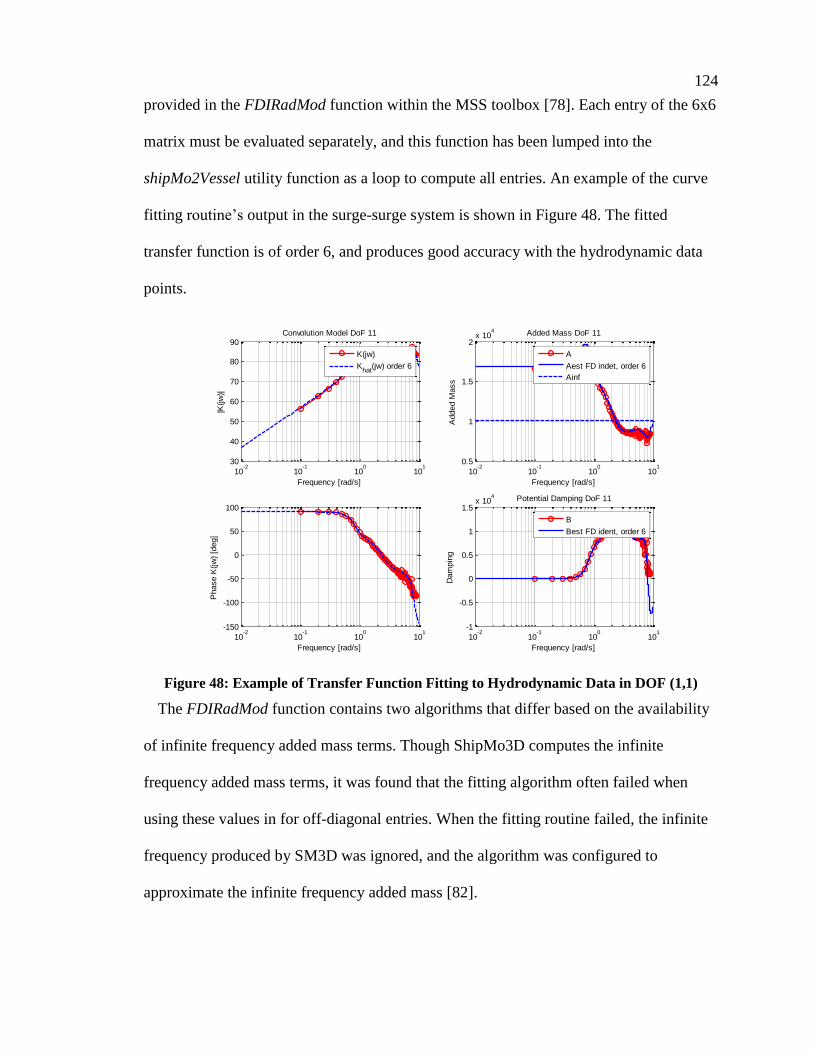
124

provided in the FDIRadMod function within the MSS toolbox [78]. Each entry of the 6x6

matrix must be evaluated separately, and this function has been lumped into the

shipMo2Vessel utility function as a loop to compute all entries. An example of the curve

fitting routine’s output in the surge-surge system is shown in Figure 48. The fitted

transfer function is of order 6, and produces good accuracy with the hydrodynamic data

points.

Figure 48: Example of Transfer Function Fitting to Hydrodynamic Data in DOF (1,1)

The FDIRadMod function contains two algorithms that differ based on the availability

of infinite frequency added mass terms. Though ShipMo3D computes the infinite

frequency added mass terms, it was found that the fitting algorithm often failed when

using these values in for off-diagonal entries. When the fitting routine failed, the infinite

frequency produced by SM3D was ignored, and the algorithm was configured to

approximate the infinite frequency added mass [82].

10-2

10-1

100

101

30

40

50

60

70

80

90

Frequency [rad/s]

|K(jw

)|

Convolution Model DoF 11

K(jw)

Khat

(jw) order 6

10-2

10-1

100

101

-150

-100

-50

0

50

100

Phase K

(jw

) [d

eg]

Frequency [rad/s]

10-2

10-1

100

101

-1

-0.5

0

0.5

1

1.5x 10

4

Frequency [rad/s]

Dam

pin

g

Potential Damping DoF 11

B

Best FD ident, order 6

10-2

10-1

100

101

0.5

1

1.5

2x 10

4

Frequency [rad/s]

Added M

ass

Added Mass DoF 11

A

Aest FD indet, order 6

Ainf

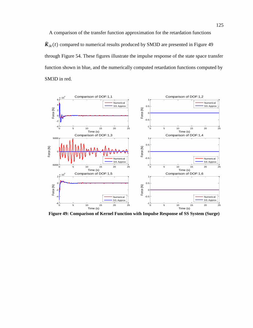
125

A comparison of the transfer function approximation for the retardation functions

𝑖𝑘(𝑡) compared to numerical results produced by SM3D are presented in Figure 49

through Figure 54. These figures illustrate the impulse response of the state space transfer

function shown in blue, and the numerically computed retardation functions computed by

SM3D in red.

Figure 49: Comparison of Kernel Function with Impulse Response of SS System (Surge)

0 5 10 15 20 25-4

-2

0

2

4

6x 10

4

Time (s)

Fo

rce

(N

)

Comparison of DOF:1,1

Numerical

SS Approx

0 5 10 15 20 25-1

-0.5

0

0.5

1

Time (s)

Fo

rce

(N

)


Numerical

SS Approx

0 5 10 15 20 25-5000

0

5000

Time (s)

Fo

rce

(N

)


Numerical

SS Approx

0 5 10 15 20 25-1

-0.5

0

0.5

1

Time (s)

Fo

rce

(N

)


Numerical

SS Approx

0 5 10 15 20 25-6

-4

-2

0

2x 10

6

Time (s)

Fo

rce

(N

)


Numerical

SS Approx

0 5 10 15 20 25-1

-0.5

0

0.5

1

Time (s)

Fo

rce

(N

)


Numerical

SS Approx

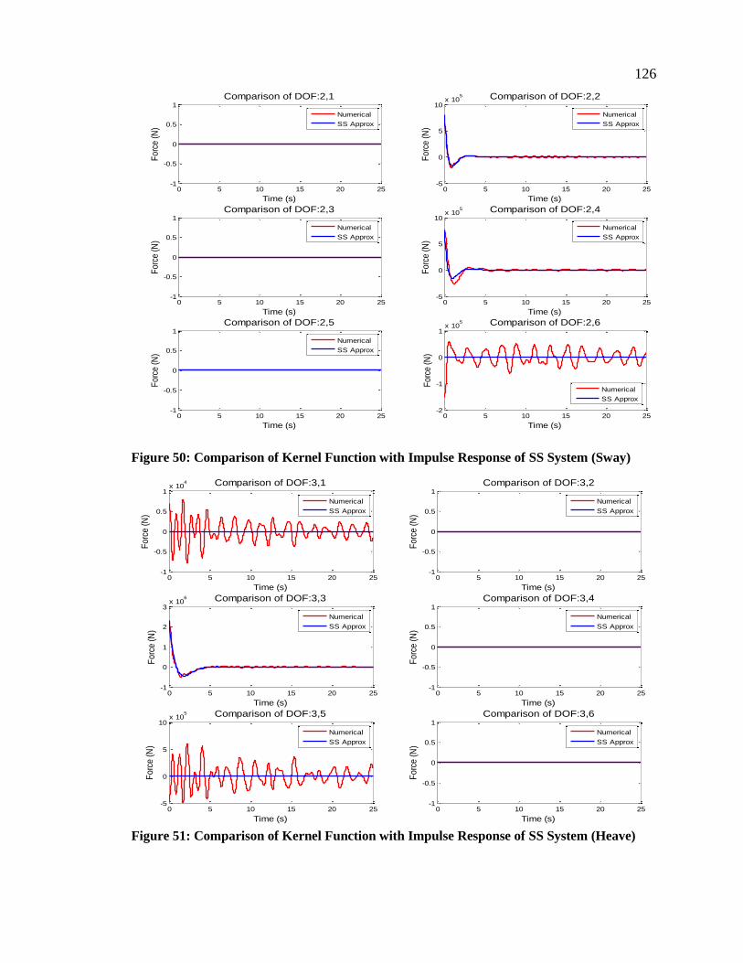
126

Figure 50: Comparison of Kernel Function with Impulse Response of SS System (Sway)

Figure 51: Comparison of Kernel Function with Impulse Response of SS System (Heave)

0 5 10 15 20 25-1

-0.5

0

0.5

1

Time (s)

Fo

rce

(N

)


Numerical

SS Approx

0 5 10 15 20 25-5

0

5

10x 10

5

Time (s)

Fo

rce

(N

)


Numerical

SS Approx

0 5 10 15 20 25-1

-0.5

0

0.5

1

Time (s)

Fo

rce

(N

)


Numerical

SS Approx

0 5 10 15 20 25-5

0

5

10x 10

5

Time (s)

Fo

rce

(N

)


Numerical

SS Approx

0 5 10 15 20 25-1

-0.5

0

0.5

1

Time (s)

Fo

rce

(N

)


Numerical

SS Approx

0 5 10 15 20 25-2

-1

0

1x 10

5

Time (s)F

orc

e (

N)


Numerical

SS Approx

0 5 10 15 20 25-1

-0.5

0

0.5

1x 10

4

Time (s)

Fo

rce

(N

)


Numerical

SS Approx

0 5 10 15 20 25-1

-0.5

0

0.5

1

Time (s)

Fo

rce

(N

)


Numerical

SS Approx

0 5 10 15 20 25-1

0

1

2

3x 10

6

Time (s)

Fo

rce

(N

)


Numerical

SS Approx

0 5 10 15 20 25-1

-0.5

0

0.5

1

Time (s)

Fo

rce

(N

)


Numerical

SS Approx

0 5 10 15 20 25-5

0

5

10x 10

5

Time (s)

Fo

rce

(N

)


Numerical

SS Approx

0 5 10 15 20 25-1

-0.5

0

0.5

1

Time (s)

Fo

rce

(N

)


Numerical

SS Approx

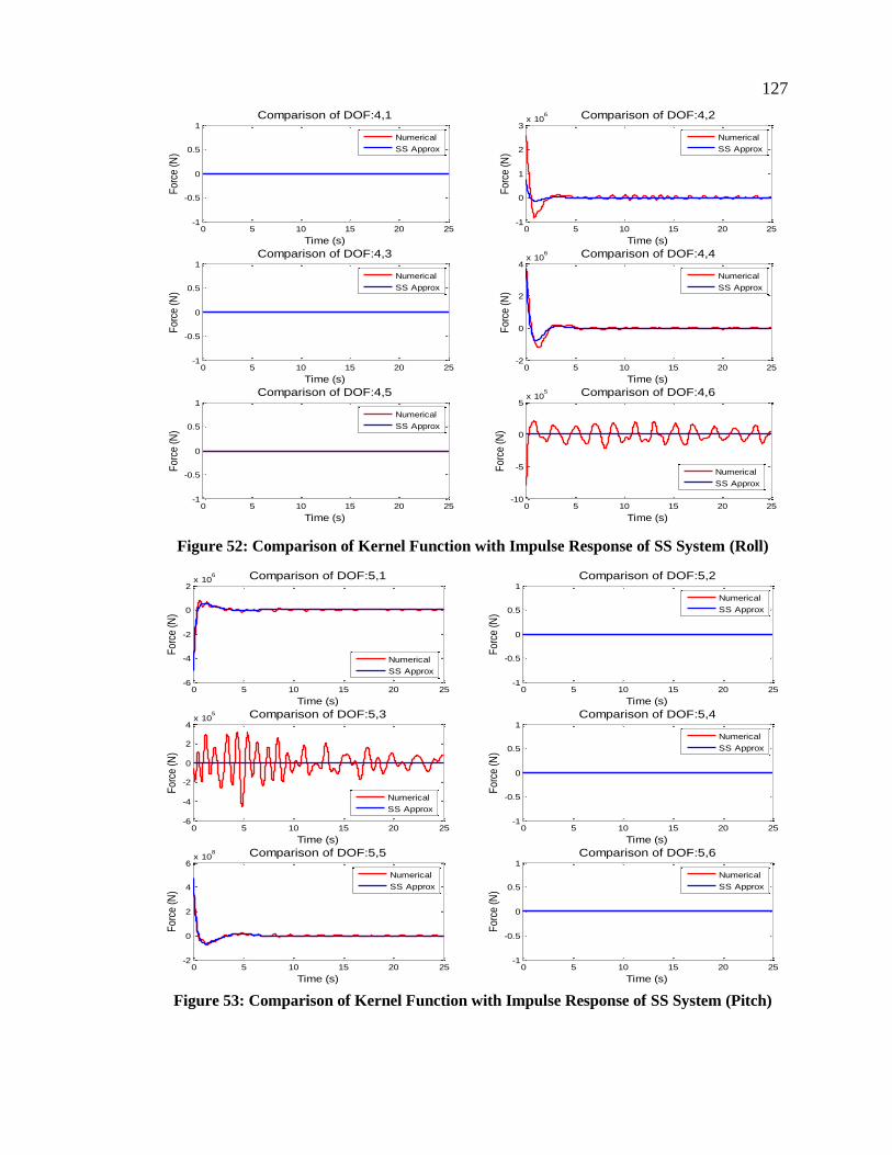
127

Figure 52: Comparison of Kernel Function with Impulse Response of SS System (Roll)

Figure 53: Comparison of Kernel Function with Impulse Response of SS System (Pitch)

0 5 10 15 20 25-1

-0.5

0

0.5

1

Time (s)

Fo

rce

(N

)


Numerical

SS Approx

0 5 10 15 20 25-1

0

1

2

3x 10

6

Time (s)

Fo

rce

(N

)


Numerical

SS Approx

0 5 10 15 20 25-1

-0.5

0

0.5

1

Time (s)

Fo

rce

(N

)


Numerical

SS Approx

0 5 10 15 20 25-2

0

2

4x 10

6

Time (s)

Fo

rce

(N

)


Numerical

SS Approx

0 5 10 15 20 25-1

-0.5

0

0.5

1

Time (s)

Fo

rce

(N

)


Numerical

SS Approx

0 5 10 15 20 25-10

-5

0

5x 10

5

Time (s)

Fo

rce

(N

)


Numerical

SS Approx

0 5 10 15 20 25-6

-4

-2

0

2x 10

6

Time (s)

Fo

rce

(N

)


Numerical

SS Approx

0 5 10 15 20 25-1

-0.5

0

0.5

1

Time (s)

Fo

rce

(N

)


Numerical

SS Approx

0 5 10 15 20 25-6

-4

-2

0

2

4x 10

5

Time (s)

Fo

rce

(N

)


Numerical

SS Approx

0 5 10 15 20 25-1

-0.5

0

0.5

1

Time (s)

Fo

rce

(N

)


Numerical

SS Approx

0 5 10 15 20 25-2

0

2

4

6x 10

8

Time (s)

Fo

rce

(N

)


Numerical

SS Approx

0 5 10 15 20 25-1

-0.5

0

0.5

1

Time (s)

Fo

rce

(N

)


Numerical

SS Approx

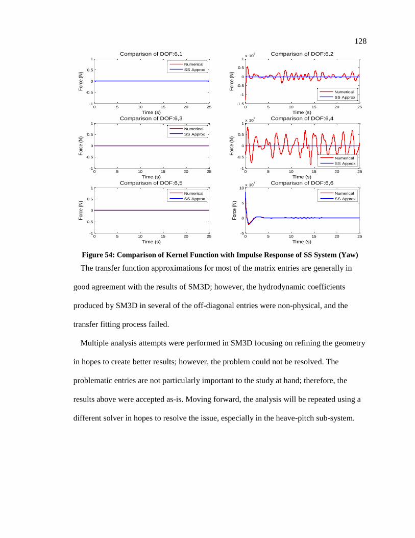
128

Figure 54: Comparison of Kernel Function with Impulse Response of SS System (Yaw)

The transfer function approximations for most of the matrix entries are generally in

good agreement with the results of SM3D; however, the hydrodynamic coefficients

produced by SM3D in several of the off-diagonal entries were non-physical, and the

transfer fitting process failed.

Multiple analysis attempts were performed in SM3D focusing on refining the geometry

in hopes to create better results; however, the problem could not be resolved. The

problematic entries are not particularly important to the study at hand; therefore, the

results above were accepted as-is. Moving forward, the analysis will be repeated using a

different solver in hopes to resolve the issue, especially in the heave-pitch sub-system.

0 5 10 15 20 25-1

-0.5

0

0.5

1

Time (s)

Fo

rce

(N

)


Numerical

SS Approx

0 5 10 15 20 25-1.5

-1

-0.5

0

0.5

1x 10

5

Time (s)

Fo

rce

(N

)


Numerical

SS Approx

0 5 10 15 20 25-1

-0.5

0

0.5

1

Time (s)

Fo

rce

(N

)


Numerical

SS Approx

0 5 10 15 20 25-1

-0.5

0

0.5

1x 10

5

Time (s)

Fo

rce

(N

)


Numerical

SS Approx

0 5 10 15 20 25-1

-0.5

0

0.5

1

Time (s)

Fo

rce

(N

)


Numerical

SS Approx

0 5 10 15 20 25-5

0

5

10x 10

7

Time (s)

Fo

rce

(N

)


Numerical

SS Approx

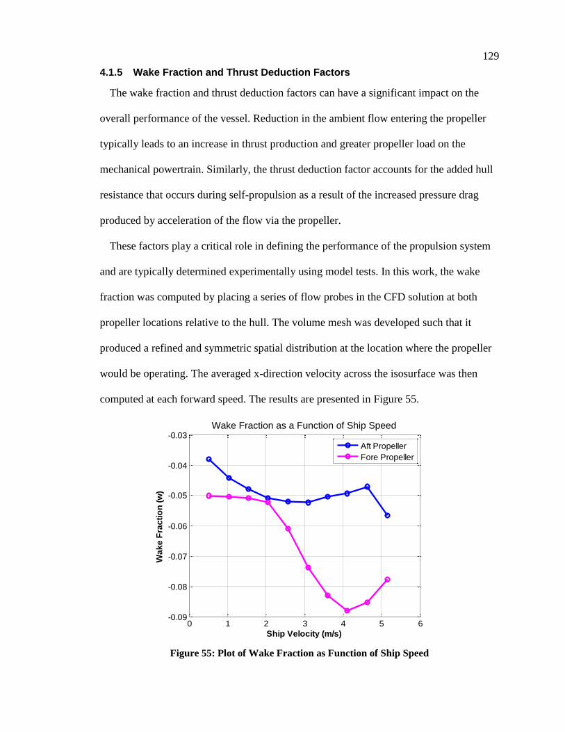
129

4.1.5 Wake Fraction and Thrust Deduction Factors

The wake fraction and thrust deduction factors can have a significant impact on the

overall performance of the vessel. Reduction in the ambient flow entering the propeller

typically leads to an increase in thrust production and greater propeller load on the

mechanical powertrain. Similarly, the thrust deduction factor accounts for the added hull

resistance that occurs during self-propulsion as a result of the increased pressure drag

produced by acceleration of the flow via the propeller.

These factors play a critical role in defining the performance of the propulsion system

and are typically determined experimentally using model tests. In this work, the wake

fraction was computed by placing a series of flow probes in the CFD solution at both

propeller locations relative to the hull. The volume mesh was developed such that it

produced a refined and symmetric spatial distribution at the location where the propeller

would be operating. The averaged x-direction velocity across the isosurface was then

computed at each forward speed. The results are presented in Figure 55.

Figure 55: Plot of Wake Fraction as Function of Ship Speed

0 1 2 3 4 5 6-0.09

-0.08

-0.07

-0.06

-0.05

-0.04

-0.03

Ship Velocity (m/s)

Wa

ke

Fra

cti

on

(w

)

Wake Fraction as a Function of Ship Speed

Aft Propeller

Fore Propeller

130

Interestingly, the wake fraction is negative for both propellers indicating that the flow

is being accelerated. Based on the placement of the thrusters, and assuming inviscid

theory, this result may intuitively makes sense because the propellers are approximately

located at the fore and aft shoulders of the hull. At these positions, the velocity has

increased and pressure has decreased. Interestingly, the original design documentation for

the Klitsa’s propulsion analysis assumed a wake fraction of 0.283, which is in stark

disagreement with the results observed with CFD.

The effect of the wake fraction is implemented using a simple lookup table that will

adjust the incoming surge velocity seen by the propeller. Depending on the direction of

travel, the fore and aft thruster effects are switched accordingly using a case-switch

subsystem.

The thrust deduction factor was slightly more difficult to resolve. The initial plan was

to perform a series of self-propulsion tests using CFD; however, complications and time

constraints did not allow. Instead, the operational data collected from the data acquisition

study was used to estimate the thrust deduction factor. Two computation methods were

used, the first using the wake fraction results directly from CFD, and the second by

averaging the wake fraction data across all the operating points as a means of

comparison. The results are tabulated in Table 13. The major issue with this approach is

the large discrepancy observed between the computed results. Environmental factors and

instrumentation error will naturally produce some variance in the predictions, making it

hard to be definitive.

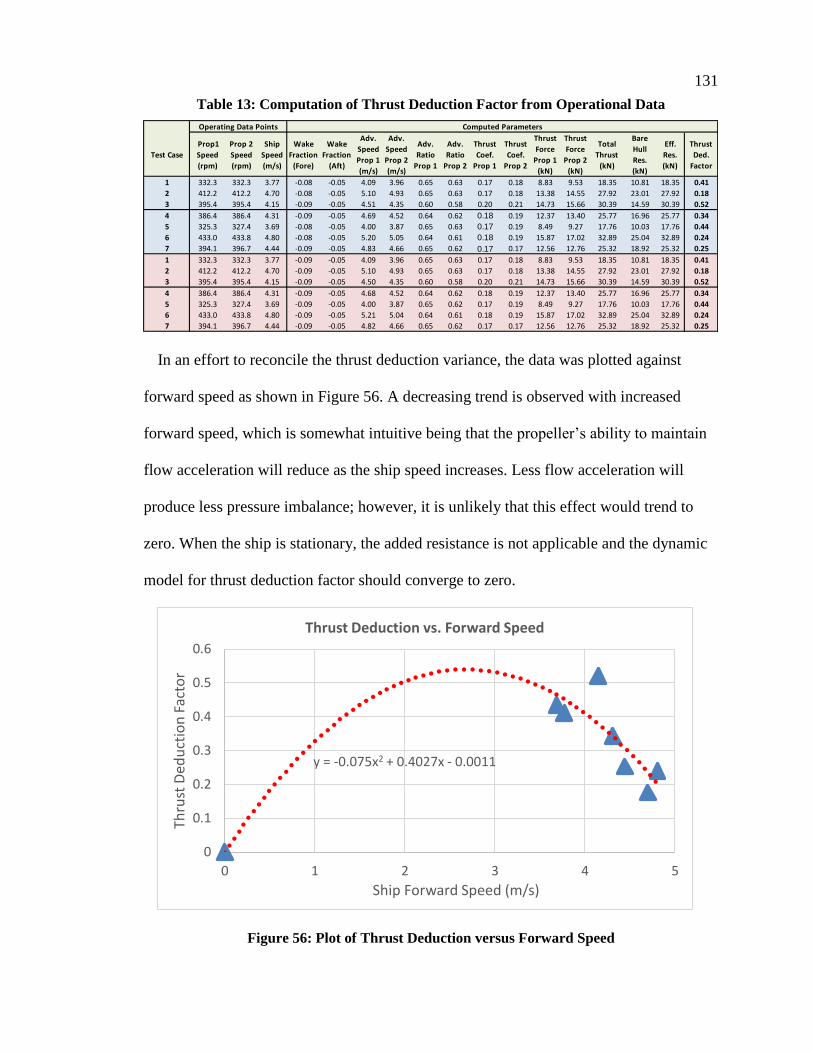
131

Table 13: Computation of Thrust Deduction Factor from Operational Data

In an effort to reconcile the thrust deduction variance, the data was plotted against

forward speed as shown in Figure 56. A decreasing trend is observed with increased

forward speed, which is somewhat intuitive being that the propeller’s ability to maintain

flow acceleration will reduce as the ship speed increases. Less flow acceleration will

produce less pressure imbalance; however, it is unlikely that this effect would trend to

zero. When the ship is stationary, the added resistance is not applicable and the dynamic

model for thrust deduction factor should converge to zero.

Figure 56: Plot of Thrust Deduction versus Forward Speed

Test Case

Prop1

Speed

(rpm)

Prop 2

Speed

(rpm)

Ship

Speed

(m/s)

Wake

Fraction

(Fore)

Wake

Fraction

(Aft)

Adv.

Speed

Prop 1

(m/s)

Adv.

Speed

Prop 2

(m/s)

Adv.

Ratio

Prop 1

Adv.

Ratio

Prop 2

Thrust

Coef.

Prop 1

Thrust

Coef.

Prop 2

Thrust

Force

Prop 1

(kN)

Thrust

Force

Prop 2

(kN)

Total

Thrust

(kN)

Bare

Hull

Res.

(kN)

Eff.

Res.

(kN)

Thrust

Ded.

Factor

1 332.3 332.3 3.77 -0.08 -0.05 4.09 3.96 0.65 0.63 0.17 0.18 8.83 9.53 18.35 10.81 18.35 0.41

2 412.2 412.2 4.70 -0.08 -0.05 5.10 4.93 0.65 0.63 0.17 0.18 13.38 14.55 27.92 23.01 27.92 0.18

3 395.4 395.4 4.15 -0.09 -0.05 4.51 4.35 0.60 0.58 0.20 0.21 14.73 15.66 30.39 14.59 30.39 0.52

4 386.4 386.4 4.31 -0.09 -0.05 4.69 4.52 0.64 0.62 0.18 0.19 12.37 13.40 25.77 16.96 25.77 0.34

5 325.3 327.4 3.69 -0.08 -0.05 4.00 3.87 0.65 0.63 0.17 0.19 8.49 9.27 17.76 10.03 17.76 0.44

6 433.0 433.8 4.80 -0.08 -0.05 5.20 5.05 0.64 0.61 0.18 0.19 15.87 17.02 32.89 25.04 32.89 0.24

7 394.1 396.7 4.44 -0.09 -0.05 4.83 4.66 0.65 0.62 0.17 0.17 12.56 12.76 25.32 18.92 25.32 0.25

1 332.3 332.3 3.77 -0.09 -0.05 4.09 3.96 0.65 0.63 0.17 0.18 8.83 9.53 18.35 10.81 18.35 0.41

2 412.2 412.2 4.70 -0.09 -0.05 5.10 4.93 0.65 0.63 0.17 0.18 13.38 14.55 27.92 23.01 27.92 0.18

3 395.4 395.4 4.15 -0.09 -0.05 4.50 4.35 0.60 0.58 0.20 0.21 14.73 15.66 30.39 14.59 30.39 0.52

4 386.4 386.4 4.31 -0.09 -0.05 4.68 4.52 0.64 0.62 0.18 0.19 12.37 13.40 25.77 16.96 25.77 0.34

5 325.3 327.4 3.69 -0.09 -0.05 4.00 3.87 0.65 0.62 0.17 0.19 8.49 9.27 17.76 10.03 17.76 0.44

6 433.0 433.8 4.80 -0.09 -0.05 5.21 5.04 0.64 0.61 0.18 0.19 15.87 17.02 32.89 25.04 32.89 0.24

7 394.1 396.7 4.44 -0.09 -0.05 4.82 4.66 0.65 0.62 0.17 0.17 12.56 12.76 25.32 18.92 25.32 0.25

Operating Data Points Computed Parameters

y = -0.075x2 + 0.4027x - 0.0011

0

0.1

0.2

0.3

0.4

0.5

0.6

0 1 2 3 4 5

Thru

st D

edu

ctio

n F

acto

r

Ship Forward Speed (m/s)

Thrust Deduction vs. Forward Speed

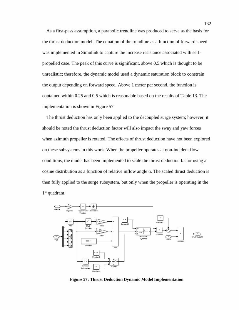
132

As a first-pass assumption, a parabolic trendline was produced to serve as the basis for

the thrust deduction model. The equation of the trendline as a function of forward speed

was implemented in Simulink to capture the increase resistance associated with self-

propelled case. The peak of this curve is significant, above 0.5 which is thought to be

unrealistic; therefore, the dynamic model used a dynamic saturation block to constrain

the output depending on forward speed. Above 1 meter per second, the function is

contained within 0.25 and 0.5 which is reasonable based on the results of Table 13. The

implementation is shown in Figure 57.

The thrust deduction has only been applied to the decoupled surge system; however, it

should be noted the thrust deduction factor will also impact the sway and yaw forces

when azimuth propeller is rotated. The effects of thrust deduction have not been explored

on these subsystems in this work. When the propeller operates at non-incident flow

conditions, the model has been implemented to scale the thrust deduction factor using a

cosine distribution as a function of relative inflow angle α. The scaled thrust deduction is

then fully applied to the surge subsystem, but only when the propeller is operating in the

1st quadrant.

Figure 57: Thrust Deduction Dynamic Model Implementation

133

Chapter 5 Modeling of AES Power System

5.1 Model Fidelity of Hybrid Power Systems

The process of modeling hybrid power systems is a balance between capturing the

dynamic response and loss characteristics of the power system while maintaining a

reasonable simulation time. The level of complexity and model order for any given study

varies depending on the analysis objectives. For system level-studies of hybrid power

systems, the dominant dynamics of each sub-component need to be well represented to

ensure that the interaction between components are fully captured. In many cases, high

frequency dynamics from power converters can be neglected with minimal impact on the

overall result.

Hybrid vehicle modeling and control optimization research often reduces powertrain

components to power loss models for rapid execution of simulations when a large design

space is being explored. The automotive powertrain analysis program PSAT, and its

predecessor Autonomie, use this approach to enable the user to rapidly assess high-level

vehicle performance for different powertrain architectures. The principle of power loss

modeling is to account for energy conversion losses, from source to consumer,

throughout a dynamic cycle. Loss models for individual powertrain components are

based on steady state efficiency maps or performance lookup tables. Components are

then assembled into a system configuration, and power flows from source to load,

through each component reducing the useful power output at each stage.

Though power loss models are invaluable to early hybrid power system sizing and

analysis, this type of modeling does not account for system dynamics and transient

losses. Recent research by Prescott [97] showed that real-time controller tuning based on

simplified power loss models may produce poor performance when deployed on a

134

detailed plant model; however, system control optimization tuning algorithms in HEVs

cannot be performed efficiently using detailed simulation models. This highlights the

importance of developing a suitable model order reduction strategy for the application.

Similarly, Jaster [17] developed a detailed power system model using SimPowerSystems

for a hybrid ship that was extremely computationally intensive, and required use of a

parallel real-time computing cluster to execute in reasonable amount of time. Even with

parallel computing, the small time-step required to resolve the switching inverters led to

unacceptable simulation times making this an unfeasible approach for any commercial

design application.

In this work, the objective is to develop a BEIPS simulation model that balances

accuracy with computational efficiency. Power loss models are used where appropriate

and more detailed models are created for components whose transient dynamics have a

large impact on overall energy consumption, thus bridging the gap between lookup table

based representation and physical system based representation. This chapter develops and

validates the individual power system component models that will be simulated as a

system in Chapter 7.

5.2 Proposed Architecture

To capitalize on British Columbia’s clean and relatively inexpensive supply of hydro-

electricity, the proposed architecture will be similar to that of a BEV. In actuality, a real

implementation would likely have backup diesel generation on-board, making this similar

architecture similar to an EREV system in automotive applications. All of the ship’s

energy needs must be supplied by the battery system. This includes delivery of AC

electrical power to service hotel loads from onboard equipment and lighting.

135

The battery provides a DC source of energy that is converted to a stable bus voltage

using a bi-directional DC/DC converter. The DC distribution grid delivers electrical

energy to the primary electric propulsion machines, while also supplying power to a

DC/AC islanding converter which produces the ship’s AC supply. Trends in ship

electrification are moving towards DC grid systems because of its advantages in [2],

1. Reducing conversion losses,

2. Flexibility in introducing energy storage, fuel cell, and solar technology,

3. Enabling of variable-speed generation,

4. Flexibility in equipment location.

The typical DC grid AES uses ICE-based electrical generation for supplying the

electrical power to the IPS. In the BEIPS architecture, these power producing elements

are completely replaced by the battery-based energy storage system. One key assumption

in this case study to note is that all existing auxiliary equipment, which includes

electrically driven pumps, fans, compressors, will remain as AC-supplied components

serviced by the DC/AC islanding converters for simplicity. Therefore, the BEIPS is

comprised of the following major components:

1. Two main electric propulsion motors

2. Bi-directional DC/DC converter

3. DC/AC islanding converter

4. Energy storage system

For reference, the architecture was illustrated back in Chapter 1 in Figure 5. The

following sections provide a detailed formulation of the simulation models created for

each of these components. The battery system requires some initial design assumptions

136

which are advised by an energy consumption analysis based on the experimental data

collected as part of the data acquisition study. The remaining components have been

developed to maintain the capacity and power requirements of the existing ship. The

capacities are summarized in the table below.

Table 14: Installed Capacity of Primary Equipment Onboard M.V. Klitsa

Component Rated Power Output

Qty. In Operation

Diesel Generator (AC Supply) 50kW/62.5kVA 1

Diesel Propulsion Engine 261kW@1800rpm 2

5.2.1 Battery Modeling

The dual polarization equivalent circuit model, shown in Figure 58, has been selected for

representation of the LTO battery pack. The fitting process for the equivalent circuit

parameters are discussed in Huria et al. [46]. In Cleary et al. [43], the authors conduct

pack-level testing then perform equivalent circuit parameter fitting based on [46] to

generate parameters for a 9.2kWh LTO battery pack. The pack consisted of eight 50Ah

modules assembled in series. The parameters are given as a function of temperature and

SOC; however, the data set is incomplete and does not cover all possible SOC and

temperature conditions. As a result, the data had to be extrapolated to complete the

battery simulation model.

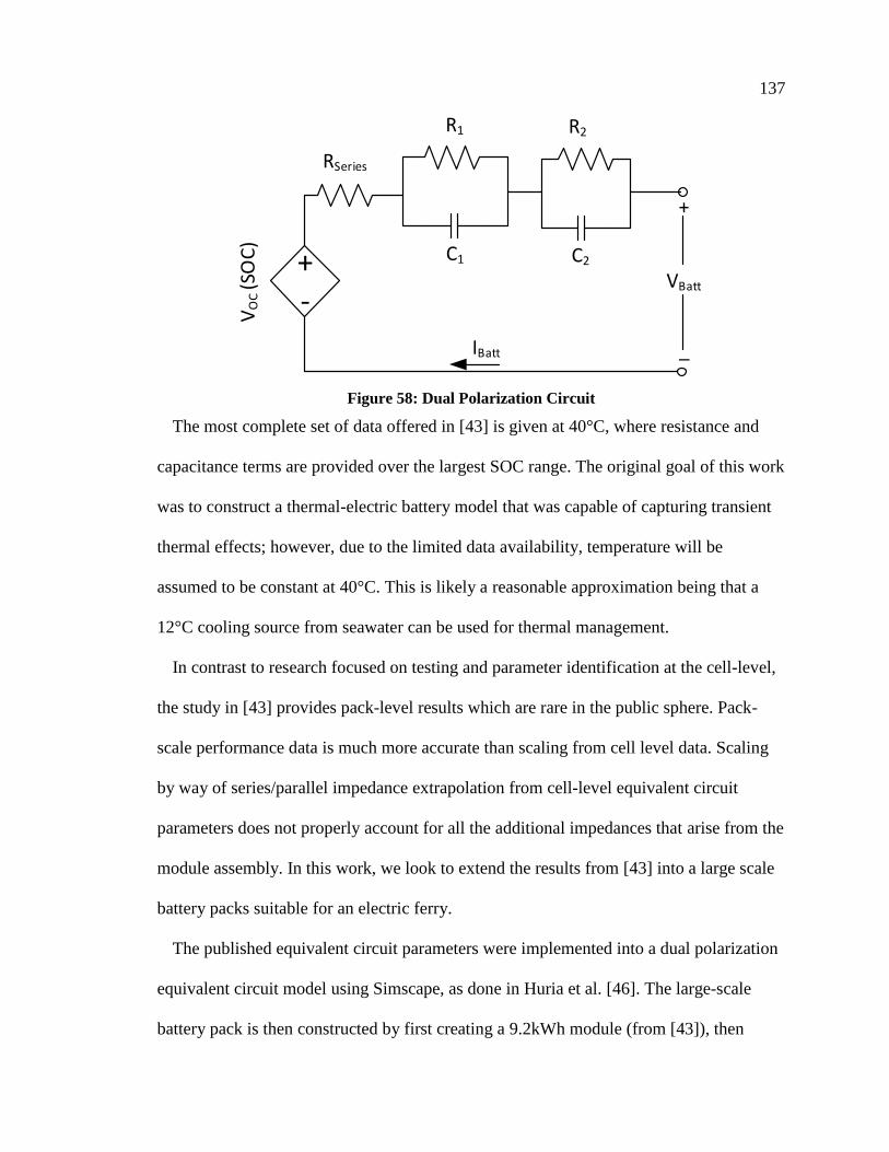
137

+-

VO

C (S

OC

)

RSeries

R1

C1

IBatt

VBatt

+

_

R2

C2

Figure 58: Dual Polarization Circuit

The most complete set of data offered in [43] is given at 40°C, where resistance and

capacitance terms are provided over the largest SOC range. The original goal of this work

was to construct a thermal-electric battery model that was capable of capturing transient

thermal effects; however, due to the limited data availability, temperature will be

assumed to be constant at 40°C. This is likely a reasonable approximation being that a

12°C cooling source from seawater can be used for thermal management.

In contrast to research focused on testing and parameter identification at the cell-level,

the study in [43] provides pack-level results which are rare in the public sphere. Pack-

scale performance data is much more accurate than scaling from cell level data. Scaling

by way of series/parallel impedance extrapolation from cell-level equivalent circuit

parameters does not properly account for all the additional impedances that arise from the

module assembly. In this work, we look to extend the results from [43] into a large scale

battery packs suitable for an electric ferry.

The published equivalent circuit parameters were implemented into a dual polarization

equivalent circuit model using Simscape, as done in Huria et al. [46]. The large-scale

battery pack is then constructed by first creating a 9.2kWh module (from [43]), then

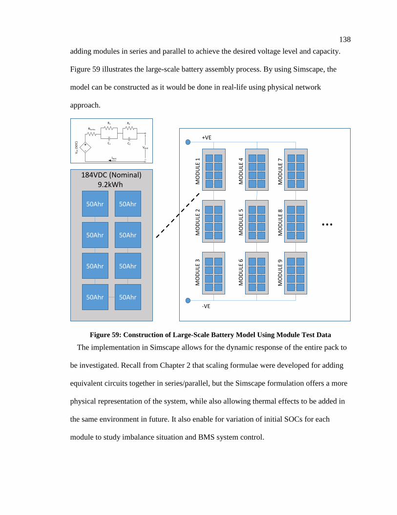
138

adding modules in series and parallel to achieve the desired voltage level and capacity.

Figure 59 illustrates the large-scale battery assembly process. By using Simscape, the

model can be constructed as it would be done in real-life using physical network

approach.

Figure 59: Construction of Large-Scale Battery Model Using Module Test Data

The implementation in Simscape allows for the dynamic response of the entire pack to

be investigated. Recall from Chapter 2 that scaling formulae were developed for adding

equivalent circuits together in series/parallel, but the Simscape formulation offers a more

physical representation of the system, while also allowing thermal effects to be added in

the same environment in future. It also enable for variation of initial SOCs for each

module to study imbalance situation and BMS system control.

50Ahr

50Ahr

50Ahr

50Ahr

50Ahr

50Ahr

50Ahr

50Ahr

184VDC (Nominal)9.2kWh

…

MO

DU

LE 1

MO

DU

LE 2

MO

DU

LE 3

MO

DU

LE 4

MO

DU

LE 5

MO

DU

LE 6

MO

DU

LE 7

MO

DU

LE 8

MO

DU

LE 9

+VE

-VE

+-

VO

C (S

OC

)

RSeries

R1

C1

IBatt

VBatt

+

_

R2

C2

139

The physical system approach allows for script-based automatic model generation,

which is a huge benefit when looking towards future in battery capacity optimization

studies. The main drawback of large-scale battery model implementation in Simscape is

the increased simulation times that can occur when co-simulating with complex systems,

especially those implemented in basic Simulink. Highly dynamic load profiles can

drastically slow down the simulation as will be discussed in section 5.2.1.2.

The equivalent circuit parameters at 40°C, published in [43], are summarized in Table

15. Interestingly, the authors did not include the OCV as a function of SOC in their

report. The data for series resistance RESR was given a function of OCV, yet no

immediate data was provided to correlate the series resistance with SOC. As a result, the

OCV versus SOC parameters had to be estimated from datasheets of a similar LTO cell.

This allowed the ESR to be estimated as a function of SOC for equivalent circuit model.

This process produced low resolution in some regions, especially at SOCs greater than

90%. Parameters that have been estimated based using the above technique are italicized

in Table 15. It should be noted that the ESR values have been averaged between their

charge and discharge values for simplicity. The original Simscape model included

individual lookup tables for charge and discharge ESR; however, this was found to cause

a numerical instability which slowed down the simulation drastically.

140

Table 15: Summary of Equivalent Circuit Parameters for 9.2kWh Module

SOC OCV (V) RESR (Ω) R1 (Ω) C1 (F) R2 (Ω) C2 (F)

0.132 169.3 0.05714 0.0246 109.8 0.058811 7203

0.232 174.6 0.05692 0.0242 207.89 0.042464 12199

0.333 179.5 0.05627 0.0205 235.4 0.03255 11025

0.434 182.2 0.05574 0.0142 296.02 0.022281 4205.2

0.534 183.4 0.05297 0.014 309.54 0.011296 3158.6

0.635 185.0 0.04831 0.0113 354.31 0.010301 2645.8

0.736 187.7 0.04834 0.0099 436.17 0.010394 2446.6

0.837 191.0 0.04779 0.0102 437.13 0.010403 2456.5

0.937 200.5 0.04779 0.0101 468.56 0.008193 2146.6

As mentioned previously, one of the major gaps in the data published in [43] relates to

the OCV versus SOC relationship. The OCV is typically calculated at a very small C-rate

(1/25C), whereas the OCV plots provided by the authors are given at 1C. The authors

appear to have confused terminal voltage with OCV in these plots in the context of the

equivalent circuit parameters. Instead of using the OCV data provided in the report, the

curves from another LTO cell provider were used as a basis for the model. Figure 60

shows a 1C discharge capacity test comparison between the 9.2kWh module presented in

Cleary et al. [43], with the model developed in Simulink. The results are within

reasonable agreement, though resolution has been lost due to the incomplete dataset.

The major benefit of the equivalent circuit model is its ability to quantify the dynamic

response of the battery system when a dynamic load profile is applied. Unfortunately, the

published information doesn’t provide a good means for direct validation for the model’s

dynamic response; however, the response can be qualitatively evaluated using an HPPC

test on the large-scale pack model once it has been designed. The following section

presents the pack specifications and the preliminary design, then the dynamic

performance is investigated using the HPPC test in section 5.2.1.2.

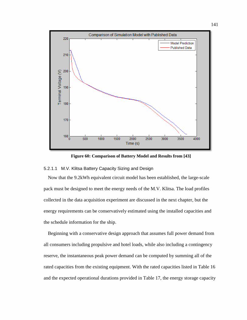
141

Figure 60: Comparison of Battery Model and Results from [43]

5.2.1.1 M.V. Klitsa Battery Capacity Sizing and Design

Now that the 9.2kWh equivalent circuit model has been established, the large-scale

pack must be designed to meet the energy needs of the M.V. Klitsa. The load profiles

collected in the data acquisition experiment are discussed in the next chapter, but the

energy requirements can be conservatively estimated using the installed capacities and

the schedule information for the ship.

Beginning with a conservative design approach that assumes full power demand from

all consumers including propulsive and hotel loads, while also including a contingency

reserve, the instantaneous peak power demand can be computed by summing all of the

rated capacities from the existing equipment. With the rated capacities listed in Table 16

and the expected operational durations provided in Table 17, the energy storage capacity

142

requirements can then be calculated based on a worst case scenario. Note that this

approach does not explicitly include an allowance for battery degradation.

Table 16: First-Pass Design Requirements for Power Output

Electric Drive 1 260kW

Electric Drive 2 260kW

Maximum Hotel Load 50kW

Contingency Allowance 30kW

Total Maximum Power Demand 600kW

Table 17: First-Pass Design for ESS Capacity Estimation

One-Way travel time 0.42h

Return Total Travel Time 0.833h

Max Energy Consumption (Return) 500kWh

From these requirements, the 9.2kWh modules were combined into series and parallel

to achieve the desired energy capacity. The high voltage DC bus is to remain constant at

750VDC to maximize the efficiency of the electric drive motors. The bi-directional

DC/DC converter will operate in boost-mode to regulate the DC grid voltage from the

battery terminals; consequently, the number of modules in series is selected such that the

maximum voltage is less than the high voltage DC bus at maximum pack voltage. This is

consistent with the commercially available the bi-directional converters such as [98].

Lastly, the expected life can be extrapolated empirically based on cycling data

available for the LTO cells. If the mean C-Rate is kept to below 3C, then data exists for

providing a preliminary pass on expected degradation. The final configuration for

achieving the desired capacity and meeting the converter constraints are given in Table

19.

143

Table 18: Single 9.2kWh Module Technical Specifications

Module Information

Nominal Voltage 184.00 V Maximum Voltage 210.00 V Minimum Voltage 160.00 V Capacity (Ah) 50.00 Ah Capacity (kWh) 9.20 Kwh

Table 19: Battery Pack Configuration and Specifications

Pack Information

Branch Series Modules 3 unit

Parallel Branches 20 unit

Total Modules 60 unit

Pack Nominal Voltage 552 V

Pack Maximum Voltage 630 V

Pack Minimum Voltage 480 V

Capacity Per Branch 9.2 kWh

Total Pack Capacity 552 kWh

Total Pack Capacity (Ah) 1000 Ah

Expected Load 275 kW

Expected Current 498.2 A

1C Current 1000 A

Expected C-rate 0.5 C

Maximum C-rate 3.00 C

5.2.1.2 Large-Scale Battery Pack Modeling and Simulation

A custom Simscape library block was created by assembling individual module blocks

into the 3S20P module configuration as dictated by the Klitsa’s energy requirements. The

resulting Simscape model, looking under the mask, is illustrated in Figure 18. The library

block tracks each module’s SOC individually, which can be averaged to get the global

SOC state. The battery pack model block also returns the total power dissipation across

all energy modules for calculating losses and estimating system efficiency. A capacity

test using the battery pack block is shown in Figure 62. The model executed sufficiently

fast, even with 60 modules simulating simultaneously, but only when current draw was

144

constant. Dynamic simulation drastically increased simulation time. For the 1C discharge

capacity test, the execution was completed in 88 seconds using the tic/toc functions

within Matlab which includes compiling time. The actual simulation time required for

3660s of simulation time was found to be 25s, giving 146:1 ratio in faster than real-time.

A plot of the SOC, terminal voltage, and current profile for the static discharge capacity

test is provided in Figure 62.

Figure 61: Construction of Battery Pack from Module Blocks in Simulink using Simscape

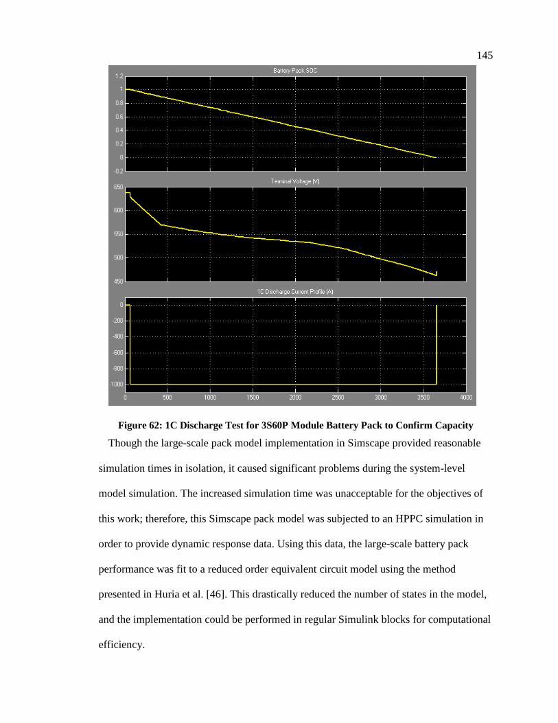
145

Figure 62: 1C Discharge Test for 3S60P Module Battery Pack to Confirm Capacity

Though the large-scale pack model implementation in Simscape provided reasonable

simulation times in isolation, it caused significant problems during the system-level

model simulation. The increased simulation time was unacceptable for the objectives of

this work; therefore, this Simscape pack model was subjected to an HPPC simulation in

order to provide dynamic response data. Using this data, the large-scale battery pack

performance was fit to a reduced order equivalent circuit model using the method

presented in Huria et al. [46]. This drastically reduced the number of states in the model,

and the implementation could be performed in regular Simulink blocks for computational

efficiency.

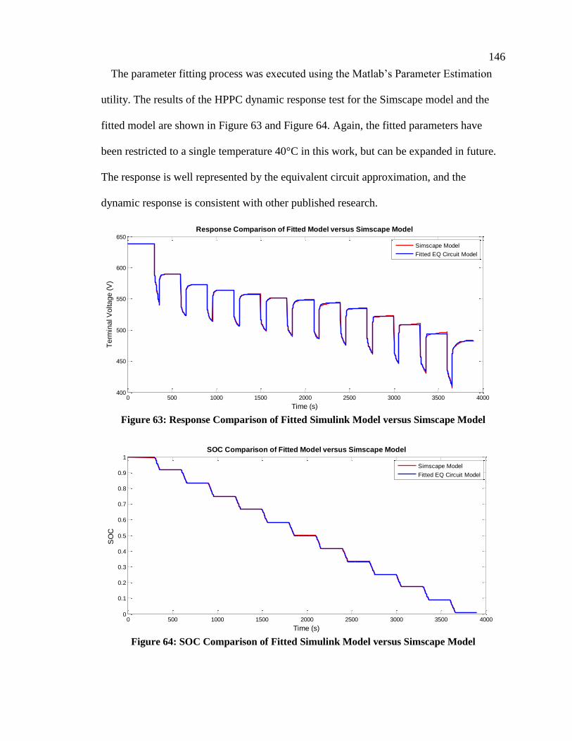
146

The parameter fitting process was executed using the Matlab’s Parameter Estimation

utility. The results of the HPPC dynamic response test for the Simscape model and the

fitted model are shown in Figure 63 and Figure 64. Again, the fitted parameters have

been restricted to a single temperature 40°C in this work, but can be expanded in future.

The response is well represented by the equivalent circuit approximation, and the

dynamic response is consistent with other published research.

Figure 63: Response Comparison of Fitted Simulink Model versus Simscape Model

Figure 64: SOC Comparison of Fitted Simulink Model versus Simscape Model

0 500 1000 1500 2000 2500 3000 3500 4000400

450

500

550

600

650

Time (s)

Te

rmin

al V

olta

ge

(V

)

Response Comparison of Fitted Model versus Simscape Model

Simscape Model

Fitted EQ Circuit Model

0 500 1000 1500 2000 2500 3000 3500 40000

0.1

0.2

0.3

0.4

0.5

0.6

0.7

0.8

0.9

1

Time (s)

SO

C

SOC Comparison of Fitted Model versus Simscape Model

Simscape Model

Fitted EQ Circuit Model

147

5.2.2 Bi-Directional DC/DC Converter Modeling

Unlike most automotive HEVs, shipboard DC installations require a fixed DC bus

voltage to control power quality and ensure full performance of all sub-system

components. The harmonics induced in the electrical system as a result of switching

power converters must be managed to minimize losses and ensure reliable operation.

Because the battery voltage will drop as it is discharged, a DC/DC converter is required

to boost the battery output to maintain a stable DC distribution voltage. In traditional

ships, the AC voltage is regulated using field control in the synchronous generators [81].

In DC grid-based AES applications, the voltage is also regulated by the electrical

generation system through controlled rectification or field excitation control in the

generator. The BEIPS system in this work differs slightly in that onboard electricity

generation has been completely replaced with stored electrical energy in the battery. As a

result, the DC/DC converter must be perform the task of voltage regulation on the

distribution DC bus.

Battery voltages are typically lower than those required by electrical drive components;

therefore, the converter operates in boost mode when supplying energy to the grid. The

system must also be capable of absorbing power in the battery; therefore, the converter

must be able to operate in buck-mode when the power flow is reversed.

Several academic papers have studied the converter topology shown in Figure 65 for

use in shipboard applications with energy storage. This converter has the advantage of

being electrically isolated as a result of the voltage transformer. This feature is critical in

the context of fault control and safety. As can be seen in circuit diagram, the converter’s

topology also includes an active-clamp system to enable zero voltage switching (ZVS)

for minimization of switching losses.

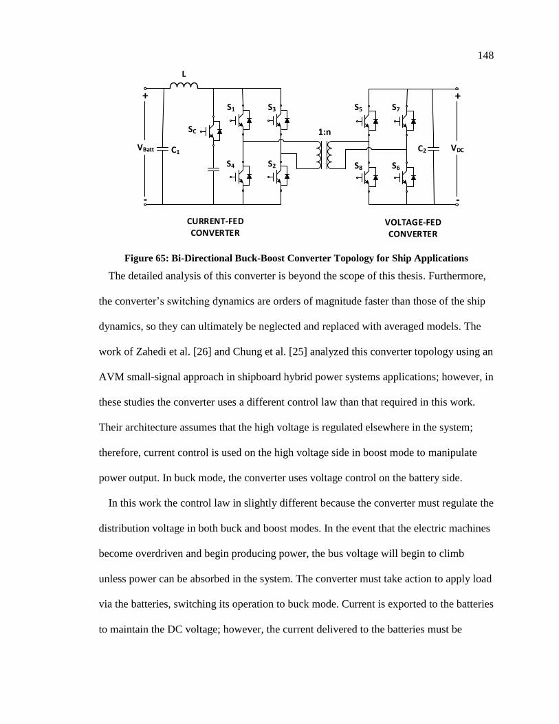
148

CURRENT-FEDCONVERTER

VBatt

+

-

+

-

VDC

SC

S1 S3

S4 S2

L

1:n

C1 C2

S5 S7

S8 S6

VOLTAGE-FEDCONVERTER

Figure 65: Bi-Directional Buck-Boost Converter Topology for Ship Applications

The detailed analysis of this converter is beyond the scope of this thesis. Furthermore,

the converter’s switching dynamics are orders of magnitude faster than those of the ship

dynamics, so they can ultimately be neglected and replaced with averaged models. The

work of Zahedi et al. [26] and Chung et al. [25] analyzed this converter topology using an

AVM small-signal approach in shipboard hybrid power systems applications; however, in

these studies the converter uses a different control law than that required in this work.

Their architecture assumes that the high voltage is regulated elsewhere in the system;

therefore, current control is used on the high voltage side in boost mode to manipulate

power output. In buck mode, the converter uses voltage control on the battery side.

In this work the control law in slightly different because the converter must regulate the

distribution voltage in both buck and boost modes. In the event that the electric machines

become overdriven and begin producing power, the bus voltage will begin to climb

unless power can be absorbed in the system. The converter must take action to apply load

via the batteries, switching its operation to buck mode. Current is exported to the batteries

to maintain the DC voltage; however, the current delivered to the batteries must be

149

regulated so to not exceed maximum C-rate. Furthermore, the maximum battery voltage

cannot be exceeded. A real application may require the use of a DC chopper for safety,

but this is unlikely to be a problem with LTO chemistry and the large capacity battery.

The current control law for the converter is described in Table 20.

Table 20: Desired Control Law BEIPS

BUCK MODE (BATTERY CHARGE)

BOOST MODEL (BATTERY DISCHARGE)

CONTROL INPUT Duty Cycle (d) Duty Cycle (d)

SYSTEM OUTPUT Voltage (VDC) Voltage (VDC)

DISTURBANCE Input Current (DC),

Battery Resistance (RBatt)

Low Voltage (VBatt),

Load Impedance (R2)

STATES Inductor Current (iL),

LV Capacitor Voltage (vC1)

Inductor Current (iL),

LV Capacitor Voltage (vC2)

Because power system stability is not being investigated in this work, this converter

can be reduced to a power losses for simplicity; however, the next logical improvement

to the power system model is to upgrade the DC/DC converter to include the average

value dynamics. As a first step, it is important to verify that the desired control law is

achievable. Chung et al. [25] derive the average value and small-signal approximations

for the converter used for controller synthesis. Here, a similar analysis is performed to

verify the desired control law.

The equations governing the converter can be expressed in average value terms,

denoted by ⟨∙⟩, where the averaged signal value is defined by,

150

⟨𝑥𝑠⟩ =1

𝑇𝑆∫ 𝑥𝑠(𝜏)𝑑𝜏

𝑡+𝑇𝑠

𝑡

( 5-1 )

Here, Ts denotes the period of the switching frequency, and xs is a general placeholder

for a signal variable. The duty cycle D and switching pattern for this converter in boost

mode is illustrated below in Figure 66.

S1, S2

S3, S4

SC

D∙ TS (1-D)∙ TS

Figure 66: Gate Signal Pattern for Bi-Directional DC/DC Converter for Boost Mode [25]

When all the switches on the current-fed bridge are turned on, the inductor is charging

and its voltage is equal to that of the battery. The voltage across the transformer is zero,

though some current will flow as a result of leakage inductance in a real transformer. In

this phase, the high voltage output capacitor C2 discharges to supply the current to the

load. When an opposing pair of switches is turned off and ignoring the active-clamp

temporarily, the energy stored in the inductor is discharged through the transformer. The

burst of current supplies the load current and recharges the output capacitor C2. Current

flows through the diodes on the voltage-fed bridge devices. The pattern is then repeated

by alternating switch pairs.

Assuming that the converter is operating in boost mode at quasi-steady state, the

application of KVL using average value analysis yields the following equation,

151

𝐿𝑑⟨𝑖𝐿⟩

𝑑𝑡≈1

𝑇𝑆[(⟨𝑣𝑏𝑎𝑡𝑡⟩ −

1

𝑛⟨𝑣𝑑𝑐⟩) (1 − 𝐷)𝑇𝑠 − ⟨𝑣𝑏𝑎𝑡𝑡⟩𝐷𝑇𝑠] ( 5-2 )

Which simplifies to,


𝑑𝑡≈ ⟨𝑣𝑏𝑎𝑡𝑡⟩ −

1

𝑛⟨𝑣𝑑𝑐⟩(1 − 𝐷) ( 5-3 )

Note the variable n represents the number of turns on the transformer secondary side.

Application of KCL on the high voltage (output) side gives the expression,

𝐶2𝑑⟨𝑣𝑑𝑐⟩

𝑑𝑡≈1

𝑇𝑆[(1

𝑛⟨𝑖𝐿⟩ −

⟨𝑣𝑑𝑐⟩

𝑅2) (1 − 𝐷)𝑇𝑠 + (−

⟨𝑣𝑏𝑎𝑡𝑡⟩

𝑅2)𝐷𝑇𝑠] ( 5-4 )

Which simplifies to,

𝐶2𝑑⟨𝑣𝑑𝑐⟩

𝑑𝑡≈1

𝑛⟨𝑖𝐿⟩(1 − 𝐷) −

⟨𝑣𝑑𝑐⟩

𝑅2 ( 5-5 )

Similarly, input current is calculated with KCL as,

𝐶1𝑑⟨𝑣𝑏𝑎𝑡𝑡⟩

𝑑𝑡≈ ⟨𝑖𝑏𝑎𝑡𝑡⟩ − ⟨𝑖𝐿⟩ ( 5-6 )

For buck mode, the gating sequence for the voltage-fed converter is shown in Figure

67. The opposing switches on the voltage-fed converter produce a reversing voltage on

the transformer winding. For a duration of DTs, power flows through the transformer and

the converter-fed bridge diodes to be stored in the inductor. When both switch pairs are

turned off, the inductor discharges stored energy to the low voltage side charging the

battery.

152

S5, S6

S7, S8

D∙ TS (1-D)∙ TS

Figure 67: Gate Signal Pattern for Bi-Directional DC/DC Converter for Buck Mode

Now assuming operation in buck mode at quasi-steady state, application of KVL using

average values analysis yields the following equation,


𝑑𝑡≈1

𝑇𝑆[(1

𝑛⟨𝑣𝑑𝑐⟩ − ⟨𝑣𝑏𝑎𝑡𝑡⟩)𝐷𝑇𝑠 − ⟨𝑣𝑏𝑎𝑡𝑡⟩(1 − 𝐷)𝑇𝑠] ( 5-7 )

This simplifies to,


𝑑𝑡≈1

𝑛⟨𝑣𝑑𝑐⟩𝐷 − ⟨𝑣𝑏𝑎𝑡𝑡⟩ ( 5-8 )

Application of KCL on the low voltage side (output) gives the expression,

𝐶1𝑑⟨𝑣𝑏𝑎𝑡𝑡⟩

𝑑𝑡≈ ⟨𝑖𝐿⟩(1 − 𝐷) −

⟨𝑣𝑏𝑎𝑡𝑡⟩

𝑅1 ( 5-9 )

The input equation is described by,

𝐶2𝑑𝑣𝑑𝑐𝑑𝑡

≈ ⟨𝑖𝑑𝑐⟩ − ⟨𝑖𝐿⟩𝑛𝐷 ( 5-10 )

The average current drawn from the high voltage source is then given by,

⟨𝑖𝐷𝐶⟩ ≈1

𝑇𝑠[⟨𝑖𝑝,𝐻𝑉⟩𝐷𝑇𝑠 + 0(1 − 𝐷)𝑇𝑠] = ⟨𝑖𝑝,𝐻𝑉⟩𝐷 ( 5-11 )

Chung et al. [25] develop the small-signal average models for these equations by

applying Taylor series and gathering first order terms. The mean values are denoted with

capital letters, and perturbations off the mean are denoted with the ∙ identifier. The

153

resulting equations from [25] are summarized in Table 21 below with DC terms removed.

Note here that,

𝐷′ = (1 − 𝐷) ( 5-12 )

Table 21: Small-signal Approximation Equations for Controller Development

Buck Mode Boost Mode

Inductor

Balance 𝐿𝑑𝑖𝐿𝑑𝑡

=1

𝑛𝐷𝑣𝑑𝑐 +

1

𝑛𝑉𝐷𝐶 − 𝑣𝑏𝑎𝑡𝑡 𝐿

𝑑𝑖𝐿𝑑𝑡= 𝑣𝑏𝑎𝑡𝑡 −

𝐷′

𝑛𝑣𝑑𝑐 +

1

𝑛𝑉𝐷𝐶

Output

Current 𝐶1𝑑𝑣𝑏𝑎𝑡𝑡𝑑𝑡

= 𝑖𝐿 −𝑣𝑏𝑎𝑡𝑡𝑅1


=𝐷′

𝑛𝑖𝐿 −

1

𝑛𝐼𝐿 −

𝑣𝑑𝑐𝑅2

Input Current 𝐶2𝑑𝑣𝑑𝑐𝑑𝑡

≈ 𝑖𝑑𝑐 − 𝑛𝐼𝐿 − 𝑛𝐷𝑖𝐿 𝐶1𝑑𝑣𝑏𝑎𝑡𝑡𝑑𝑡

≈ 𝑖𝑏𝑎𝑡𝑡 − 𝑖𝐿

Transformer

Current 𝑖𝑠 =

1

𝑛𝑖𝐿 𝑖𝑠 =

1

𝑛𝑖𝐿𝐷′

Using these equation, we can develop transfer functions that can be developed based on

the desired control law. This is done in Appendix B, along with a verification of

controllability using numerical values from the converters studied in [25] and [26]. The

transfer functions for bus voltage regulation in both buck and boost modes are presented

in Table 22.

Table 22: HVDC Control Transfer Function for Buck and Boost Mode

Transfer

Function Buck Mode Boost Mode

𝐺𝑣𝑑𝑐𝑑(𝑠) −(𝑠𝑛𝐿𝐼𝐿 + 𝐷𝑉𝐷𝐶)

𝑠2𝐿𝐶2 + 𝐷2

𝑅2(𝐷′𝑉𝐷𝐶 − 𝑛𝐼𝐿𝑠𝐿)

(𝑠2𝐿𝑛2𝐶2𝑅2 + 𝑠𝐿𝑛2 + 𝑅2𝐷′2)

Design of the converter and development of the controller will constitute future work.

For now, the task is to develop a reasonable efficiency map for the converter for our

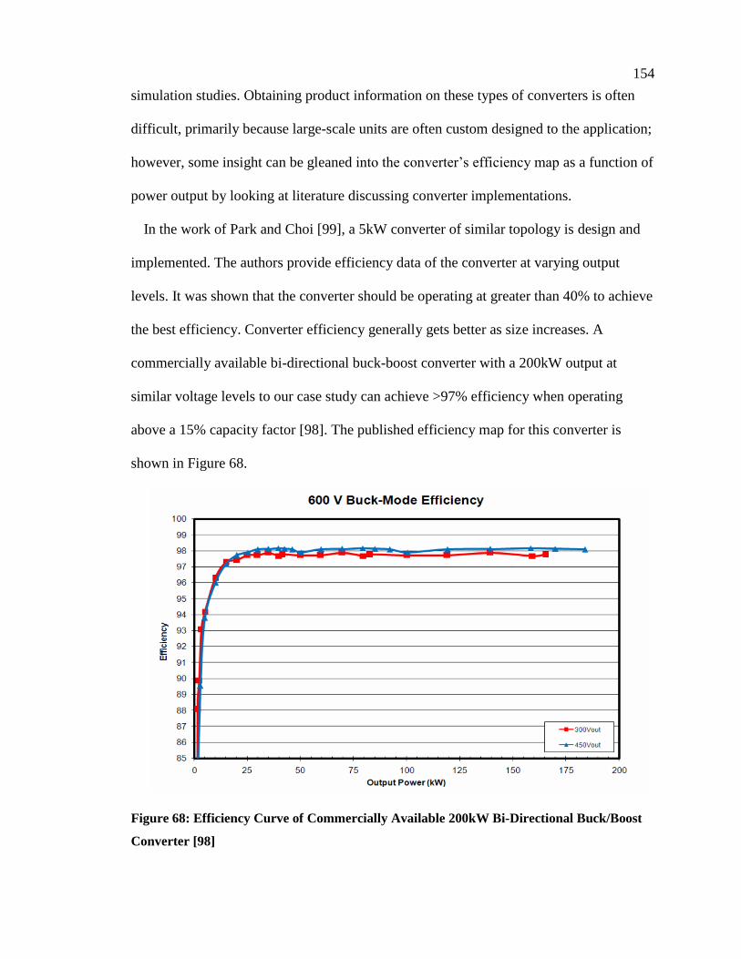
154

simulation studies. Obtaining product information on these types of converters is often

difficult, primarily because large-scale units are often custom designed to the application;

however, some insight can be gleaned into the converter’s efficiency map as a function of

power output by looking at literature discussing converter implementations.

In the work of Park and Choi [99], a 5kW converter of similar topology is design and

implemented. The authors provide efficiency data of the converter at varying output

levels. It was shown that the converter should be operating at greater than 40% to achieve

the best efficiency. Converter efficiency generally gets better as size increases. A

commercially available bi-directional buck-boost converter with a 200kW output at

similar voltage levels to our case study can achieve >97% efficiency when operating

above a 15% capacity factor [98]. The published efficiency map for this converter is

shown in Figure 68.

Figure 68: Efficiency Curve of Commercially Available 200kW Bi-Directional Buck/Boost

Converter [98]

155

Because the ship’s operational profile has significant swings in power output, it is

essential that the capacity factor of the converter be investigated to ensure maximum

efficiency over the entire load profile. In berth, the ship’s battery will be connected to the

charging infrastructure; however, the converter will still supply the main propulsive and

hotel loads. Based on observations from the data acquisition study, a high output and low

output scenario were developed to investigate capacity factor during both transit and

while in berth. Table 23 and Table 24 show a comparison between use of a single 600kW

converter, and the use of two 300kW converters assuming the same efficiency map as

presented in Figure 68. With a single converter operating while in berth, the low capacity

factor will lead to a reduction in overall system efficiency. In contrast, the use of two

converters enables a higher potential for maximizing system efficiency at low loads by

boosting the capacity factor.

Table 23: Low and High Load Comparison for M.V. Klitsa with Single Converter

Low Operating Condition - In Transit High Operating Condition - In Transit

Converter Rating 600 kW Converter Rating 600 kW

Engine 1 Low Output (40%) 100 kW Engine 1 High Output (80%) 200 kW


Low Hotel Load 10 kW High Hotel Load 35 kW

Low Load Operational 210 kW High Load Operational 435 kW

Capacity Factor 0.35 Capacity Factor 0.73

Low Operating Condition - In Berth High Operating Condition - In Berth





Low Load Operational 60 kW Low Load Operational 110 kW

Capacity Factor 0.1 Capacity Factor 0.183

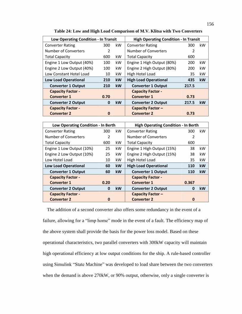
156

Table 24: Low and High Load Comparison of M.V. Klitsa with Two Converters

Low Operating Condition - In Transit High Operating Condition - In Transit


Number of Converters 2 Number of Converters 2

Total Capacity 600 kW Total Capacity 600



Low Constant Hotel Load 10 kW High Hotel Load 35 kW


Converter 1 Output 210 kW Converter 1 Output 217.5

Capacity Factor - Converter 1 0.70


Converter 2 Output 0 kW Converter 2 Output 217.5 kW

Capacity Factor - Converter 2 0

Capacity Factor – Converter 2 0.73

Low Operating Condition - In Berth High Operating Condition - In Berth


Number of Converters 2 Number of Converters 2

Total Capacity 600 kW Total Capacity 600





Converter 1 Output 60 kW Converter 1 Output 110 kW



Converter 2 Output 0 kW Converter 2 Output 0 kW

Capacity Factor - Converter 2 0

Capacity Factor – Converter 2 0

The addition of a second converter also offers some redundancy in the event of a

failure, allowing for a “limp home” mode in the event of a fault. The efficiency map of

the above system shall provide the basis for the power loss model. Based on these

operational characteristics, two parallel converters with 300kW capacity will maintain

high operational efficiency at low output conditions for the ship. A rule-based controller

using Simulink “State Machine” was developed to load share between the two converters

when the demand is above 270kW, or 90% output, otherwise, only a single converter is

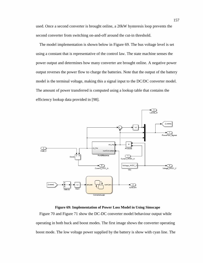
157

used. Once a second converter is brought online, a 20kW hysteresis loop prevents the

second converter from switching on-and-off around the cut-in threshold.

The model implementation is shown below in Figure 69. The bus voltage level is set

using a constant that is representative of the control law. The state machine senses the

power output and determines how many converter are brought online. A negative power

output reverses the power flow to charge the batteries. Note that the output of the battery

model is the terminal voltage, making this a signal input to the DC/DC converter model.

The amount of power transferred is computed using a lookup table that contains the

efficiency lookup data provided in [98].

Figure 69: Implementation of Power Loss Model in Using Simscape

Figure 70 and Figure 71 show the DC-DC converter model behaviour output while

operating in both buck and boost modes. The first image shows the converter operating

boost mode. The low voltage power supplied by the battery is show with cyan line. The

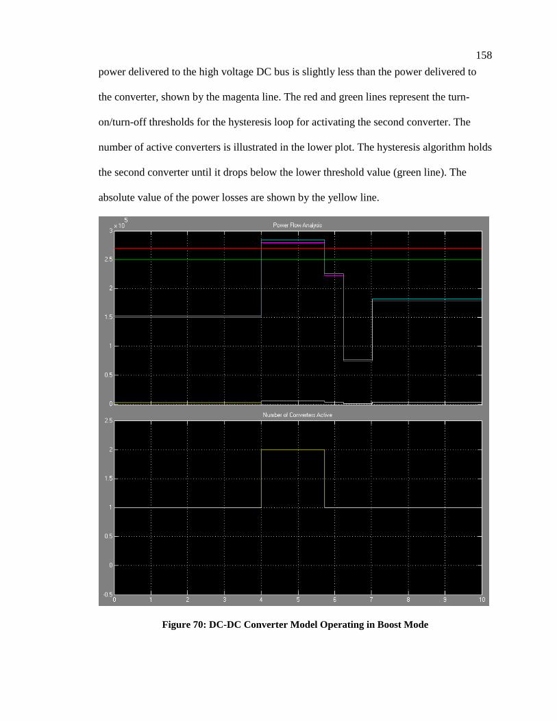
158

power delivered to the high voltage DC bus is slightly less than the power delivered to

the converter, shown by the magenta line. The red and green lines represent the turn-

on/turn-off thresholds for the hysteresis loop for activating the second converter. The

number of active converters is illustrated in the lower plot. The hysteresis algorithm holds

the second converter until it drops below the lower threshold value (green line). The

absolute value of the power losses are shown by the yellow line.

Figure 70: DC-DC Converter Model Operating in Boost Mode

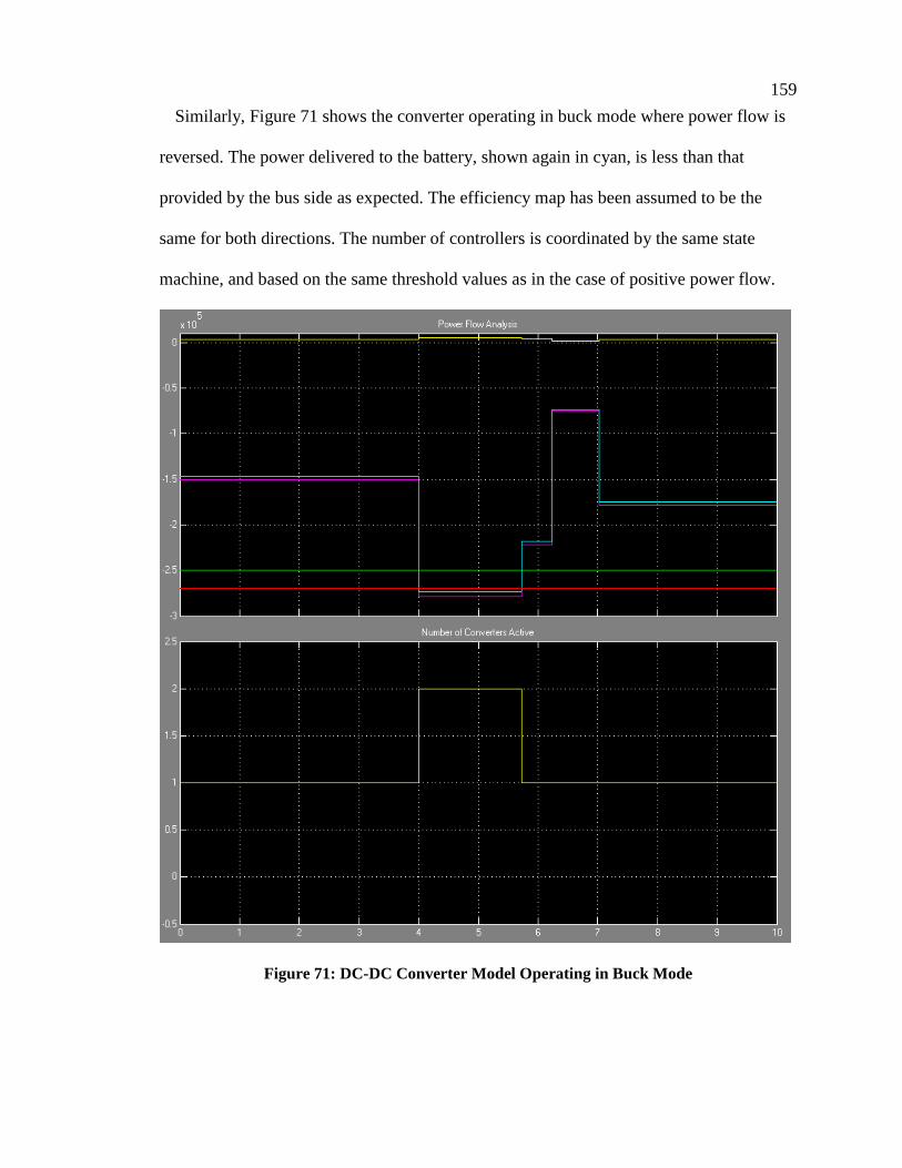
159

Similarly, Figure 71 shows the converter operating in buck mode where power flow is

reversed. The power delivered to the battery, shown again in cyan, is less than that

provided by the bus side as expected. The efficiency map has been assumed to be the

same for both directions. The number of controllers is coordinated by the same state

machine, and based on the same threshold values as in the case of positive power flow.

Figure 71: DC-DC Converter Model Operating in Buck Mode

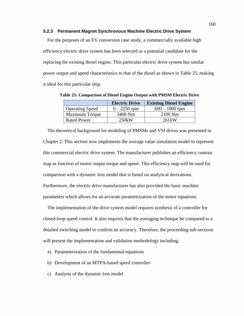
160

5.2.3 Permanent Magnet Synchronous Machine Electric Drive System

For the purposes of an EV conversion case study, a commercially available high

efficiency electric drive system has been selected as a potential candidate for the

replacing the existing diesel engine. This particular electric drive system has similar

power output and speed characteristics to that of the diesel as shown in Table 25, making

it ideal for this particular ship.

Table 25: Comparison of Diesel Engine Output with PMSM Electric Drive

Electric Drive Existing Diesel Engine

Operating Speed 0 – 2250 rpm 600 – 1800 rpm

Maximum Torque 3400 Nm 2100 Nm

Rated Power 250kW 261kW

The theoretical background for modeling of PMSMs and VSI drives was presented in

Chapter 2. This section now implements the average value simulation model to represent

this commercial electric drive system. The manufacturer publishes an efficiency contour

map as function of motor output torque and speed. This efficiency map will be used for

comparison with a dynamic loss model that is based on analytical derivations.

Furthermore, the electric drive manufacturer has also provided the basic machine

parameters which allows for an accurate parametrization of the motor equations.

The implementation of the drive system model requires synthesis of a controller for

closed-loop speed control. It also requires that the averaging technique be compared to a

detailed switching model to confirm its accuracy. Therefore, the proceeding sub-sections

will present the implementation and validation methodology including,

a) Parameterization of the fundamental equations

b) Development of an MTPA-based speed controller

c) Analysis of the dynamic loss model

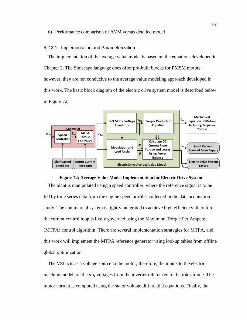
161

d) Performance comparison of AVM versus detailed model

5.2.3.1 Implementation and Parameterization

The implementation of the average value model is based on the equations developed in

Chapter 2. The Simscape language does offer pre-built blocks for PMSM motors;

however, they are not conducive to the average value modeling approach developed in

this work. The basic block diagram of the electric drive system model is described below

in Figure 72.

Controller

Electric Drive Average Value Model

D-Q Motor Voltage Equations

Torque Production Equation

Modulation and Load Angle

Calculate DC Current From

Torque and Losses Using Power

Balance

Speed Controller

MTPA Torque

Controller

Mechanical Equation of Motion Including Propeller

Torque

Input Current Sourced From Supply

Electric Drive System Losses

Shaft Speed Feedback

Motor Current Feedback

Idqo Tmtr

VdqoTrefωref

M

δ

Idc

Ploss

Figure 72: Average Value Model Implementation for Electric Drive System

The plant is manipulated using a speed controller, where the reference signal is to be

fed by time series data from the engine speed profiles collected in the data acquisition

study. The commercial system is tightly integrated to achieve high efficiency; therefore,

the current control loop is likely governed using the Maximum Torque Per Ampere

(MTPA) control algorithm. There are several implementation strategies for MTPA, and

this work will implement the MTPA reference generator using lookup tables from offline

global optimization.

The VSI acts as a voltage source to the motor; therefore, the inputs to the electric

machine model are the d-q voltages from the inverter referenced to the rotor frame. The

motor current is computed using the stator voltage differential equations. Finally, the

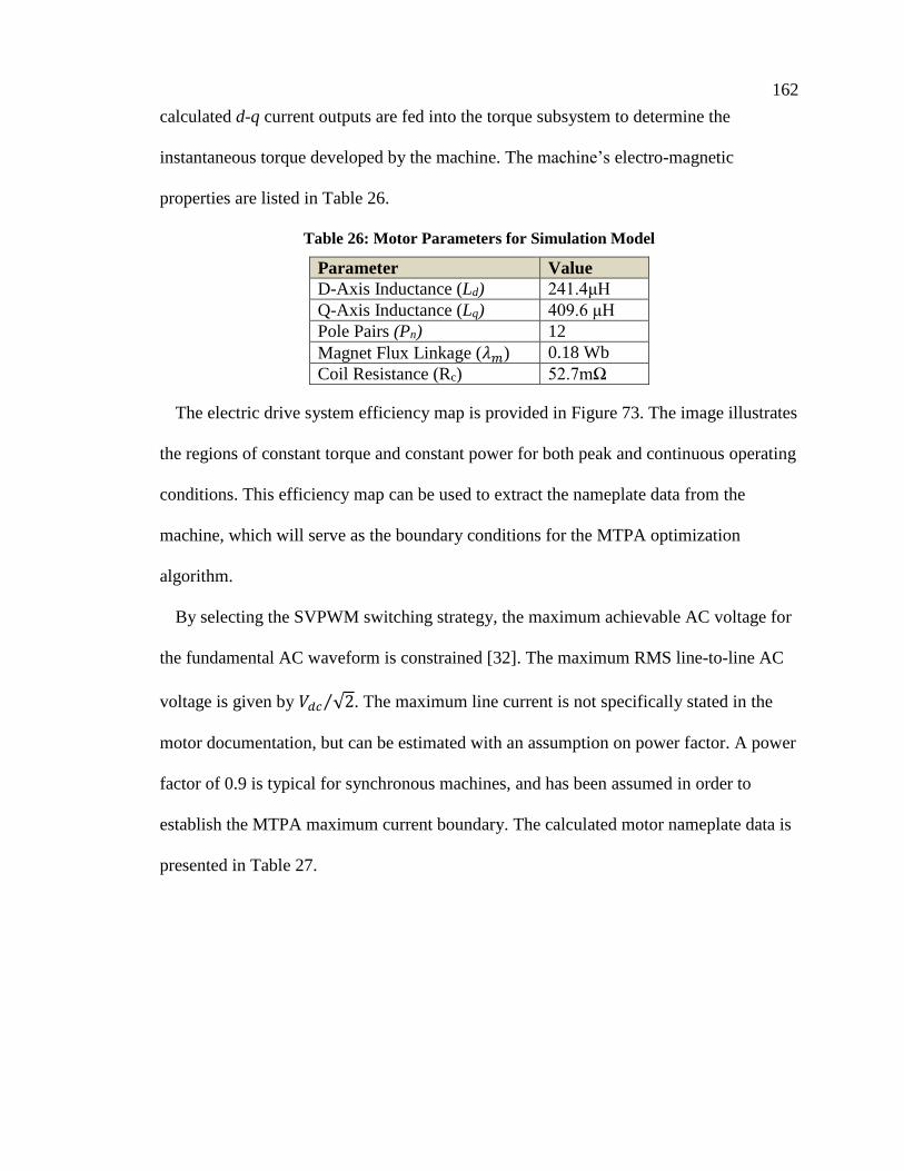
162

calculated d-q current outputs are fed into the torque subsystem to determine the

instantaneous torque developed by the machine. The machine’s electro-magnetic

properties are listed in Table 26.

Table 26: Motor Parameters for Simulation Model

Parameter Value

D-Axis Inductance (Ld) 241.4μH

Q-Axis Inductance (Lq) 409.6 μH

Pole Pairs (Pn) 12

Magnet Flux Linkage (𝜆𝑚) 0.18 Wb

Coil Resistance (Rc) 52.7mΩ

The electric drive system efficiency map is provided in Figure 73. The image illustrates

the regions of constant torque and constant power for both peak and continuous operating

conditions. This efficiency map can be used to extract the nameplate data from the

machine, which will serve as the boundary conditions for the MTPA optimization

algorithm.

By selecting the SVPWM switching strategy, the maximum achievable AC voltage for

the fundamental AC waveform is constrained [32]. The maximum RMS line-to-line AC

voltage is given by 𝑉𝑑𝑐 √2⁄ . The maximum line current is not specifically stated in the

motor documentation, but can be estimated with an assumption on power factor. A power

factor of 0.9 is typical for synchronous machines, and has been assumed in order to

establish the MTPA maximum current boundary. The calculated motor nameplate data is

presented in Table 27.

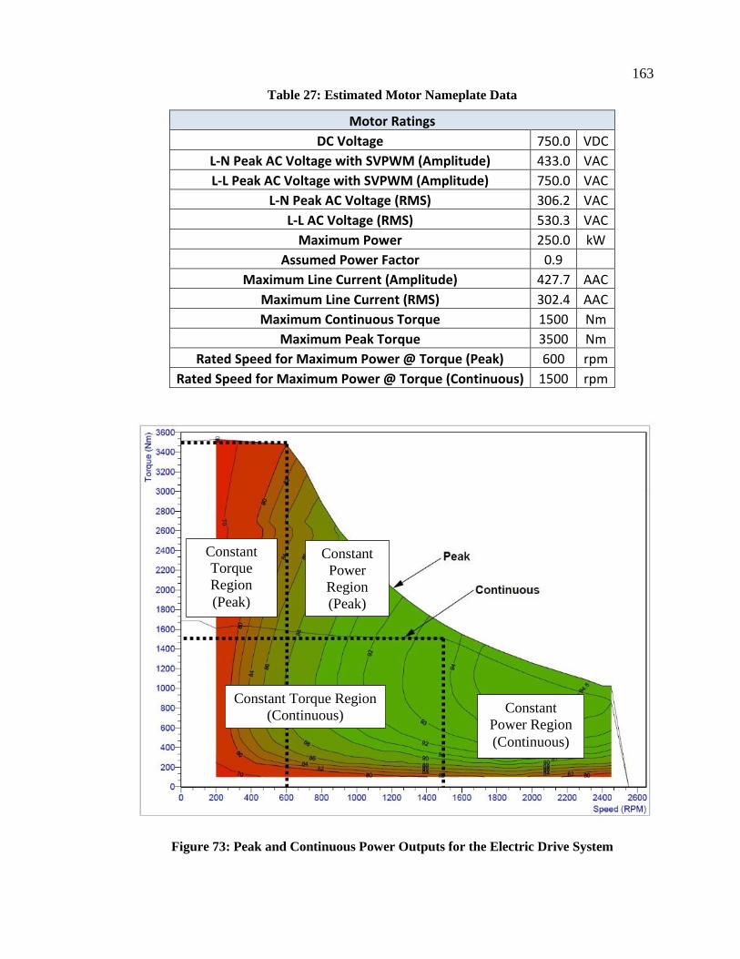
163

Table 27: Estimated Motor Nameplate Data

Motor Ratings

DC Voltage 750.0 VDC

L-N Peak AC Voltage with SVPWM (Amplitude) 433.0 VAC

L-L Peak AC Voltage with SVPWM (Amplitude) 750.0 VAC

L-N Peak AC Voltage (RMS) 306.2 VAC

L-L AC Voltage (RMS) 530.3 VAC

Maximum Power 250.0 kW

Assumed Power Factor 0.9

Maximum Line Current (Amplitude) 427.7 AAC

Maximum Line Current (RMS) 302.4 AAC

Maximum Continuous Torque 1500 Nm

Maximum Peak Torque 3500 Nm

Rated Speed for Maximum Power @ Torque (Peak) 600 rpm

Rated Speed for Maximum Power @ Torque (Continuous) 1500 rpm

Figure 73: Peak and Continuous Power Outputs for the Electric Drive System

Constant

Power Region

(Continuous)

Constant

Torque

Region

(Peak)

Constant Torque Region

(Continuous)

Constant

Power

Region

(Peak)

164

Details relating to the VSI’s switching devices and their switching frequency are

unknown, as they were not divulged by the manufacturer. The switching carrier

frequency has been assumed to be constant at 10kHz. To properly parameterize the

semiconductor loss model for the inverter, several pieces of information are required

from the device datasheets. Without the exact model number for the true semiconductor

devices, parameters have been taken from datasheets of another IGBT device with similar

power ratings. The Infineon FZ600R12KE4 IGBT has suitable power ratings for the

application, and a copy of the datasheet can be found in Appendix C. The relevant

parameters for the semiconductor loss model are summarized in Table 28. It will be

shown later that these parameters provide reasonable results in comparison to the

published efficiency map.

Table 28: IGBT Parameters for Loss Estimation

IGBT Datasheet Parameters

𝑉𝑟𝑒𝑓 1200 V

𝐼𝑟𝑒𝑓 600 A

𝑓𝑠 10 kHz

𝑉𝐷𝐶 750 V

𝐼𝐿 427.7 A

𝐸𝑜𝑛,𝐼 50 mJ

𝐸off,𝐼 75 mJ

𝐸off,𝐷 42 mJ

𝑉𝐶𝐸,0 2 V

𝑅𝐶𝐸 0.003 Ω

𝑉𝐹,0 0.6 V

𝑅𝐹 0.003 Ω

The electric drive system has nine output phases, where each phase is split across three

semiconductor devices to reduce the current seen by switching devices and the stator

coils as illustrated in Figure 74. This produces higher efficiency power conversion at the

expense of increased complexity and manufacturing cost.

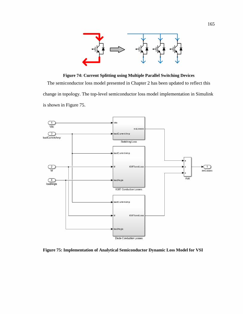
165

Figure 74: Current Splitting using Multiple Parallel Switching Devices

The semiconductor loss model presented in Chapter 2 has been updated to reflect this

change in topology. The top-level semiconductor loss model implementation in Simulink

is shown in Figure 75.

Figure 75: Implementation of Analytical Semiconductor Dynamic Loss Model for VSI

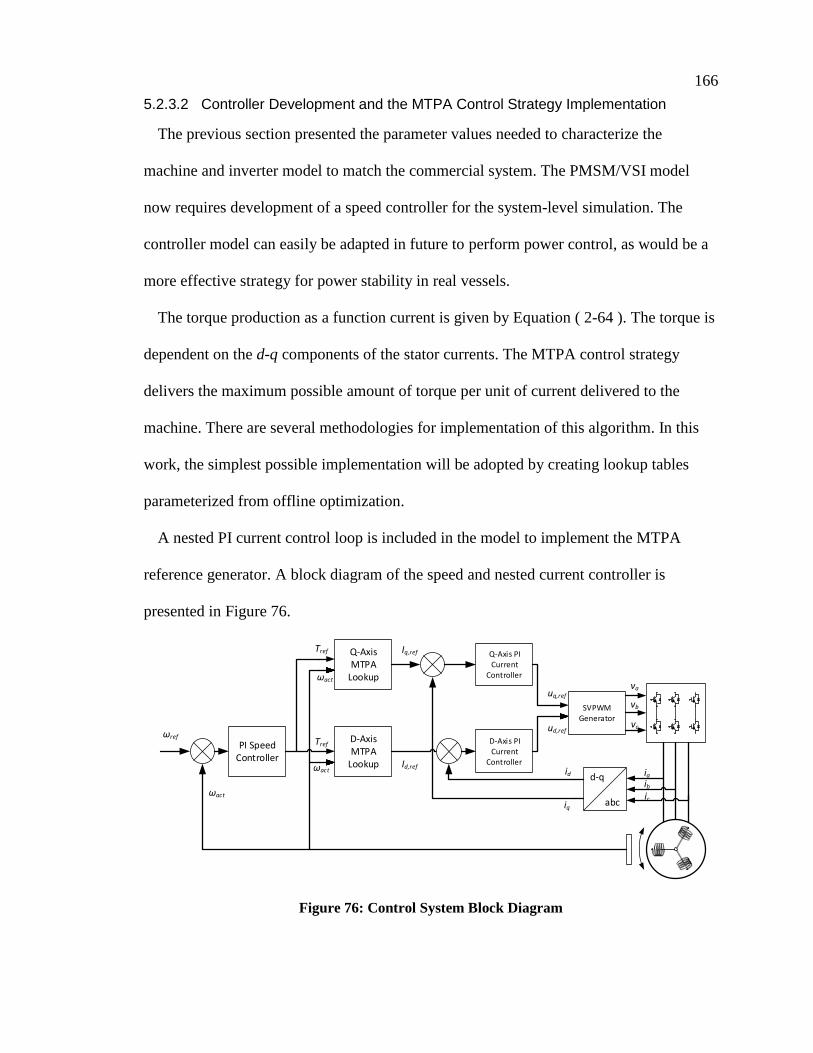
166

5.2.3.2 Controller Development and the MTPA Control Strategy Implementation

The previous section presented the parameter values needed to characterize the

machine and inverter model to match the commercial system. The PMSM/VSI model

now requires development of a speed controller for the system-level simulation. The

controller model can easily be adapted in future to perform power control, as would be a

more effective strategy for power stability in real vessels.

The torque production as a function current is given by Equation ( 2-64 ). The torque is

dependent on the d-q components of the stator currents. The MTPA control strategy

delivers the maximum possible amount of torque per unit of current delivered to the

machine. There are several methodologies for implementation of this algorithm. In this

work, the simplest possible implementation will be adopted by creating lookup tables

parameterized from offline optimization.

A nested PI current control loop is included in the model to implement the MTPA

reference generator. A block diagram of the speed and nested current controller is

presented in Figure 76.

PI Speed Controller

D-AxisMTPA

Lookup

Q-AxisMTPA

Lookup

Iq,ref

Id,ref

Tref

SVPWMGenerator

abc

d-q

uq,ref

ud,ref

iaibic

iq

id

va

vb

vc

Q-Axis PI Current

Controller

D-Axis PI Current

Controller

ωact

ωref

ωact

Tref

ωact

Figure 76: Control System Block Diagram

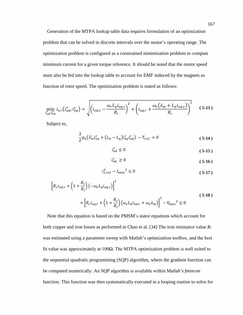
167

Generation of the MTPA lookup table data requires formulation of an optimization

problem that can be solved in discrete intervals over the motor’s operating range. The

optimization problem is configured as a constrained minimization problem to compute

minimum current for a given torque reference. It should be noted that the motor speed

must also be fed into the lookup table to account for EMF induced by the magnets as

function of rotor speed. The optimization problem is stated as follows:

min𝑖𝑜𝑑𝑟 ,𝑖𝑜𝑞

𝑟𝑖𝑠,𝑟(𝑖𝑜𝑑

𝑟 , 𝑖𝑜𝑞𝑟 ) = √(𝑖𝑜𝑑,𝑟 −

𝜔𝑟𝐿𝑞𝑖𝑜𝑞,𝑟

𝑅𝑖)2

+ (𝑖𝑜𝑞,𝑟 +𝜔𝑟(𝜆𝑚 + 𝐿𝑑𝑖𝑜𝑑,𝑟)

𝑅𝑖)

2

( 5-13 )

Subject to,

3

2𝑝𝑛(𝜆𝑚

′ 𝑖𝑜𝑞𝑟 + (𝐿𝑑 − 𝐿𝑞)𝑖𝑜𝑞

𝑟 𝑖𝑜𝑑𝑟 ) − 𝑇𝑟𝑒𝑓, = 0 ( 5-14 )

𝑖𝑜𝑑𝑟 ≤ 0 ( 5-15 )

𝑖𝑜𝑞𝑟 ≥ 0 ( 5-16 )

𝑖𝑠,𝑟𝑒𝑓2 − 𝐼𝑚𝑎𝑥

2 ≤ 0 ( 5-17 )

[𝑅𝑐𝑖𝑜𝑑,𝑟 + (1 +𝑅𝑐𝑅𝑖) (−𝜔𝑒𝐿𝑞𝑖𝑜𝑞,𝑟)]

2

+ [𝑅𝑐𝑖𝑜𝑞,𝑟 + (1 +𝑅𝑐𝑅𝑖) (𝜔𝑒𝐿𝑑𝑖𝑜𝑑,𝑟 +𝜔𝑒𝜆𝑚)]

2

− 𝑉𝑚𝑎𝑥2 ≤ 0

( 5-18 )

Note that this equation is based on the PMSM’s stator equations which account for

both copper and iron losses as performed in Chao et al. [34] The iron resistance value Ri

was estimated using a parameter sweep with Matlab’s optimization toolbox, and the best

fit value was approximately at 100Ω. The MTPA optimization problem is well suited to

the sequential quadratic programming (SQP) algorithm, where the gradient function can

be computed numerically. An SQP algorithm is available within Matlab’s fmincon

function. This function was then systematically executed in a looping routine to solve for

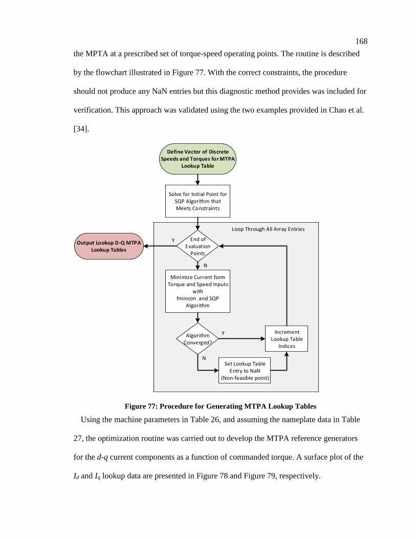
168

the MPTA at a prescribed set of torque-speed operating points. The routine is described

by the flowchart illustrated in Figure 77. With the correct constraints, the procedure

should not produce any NaN entries but this diagnostic method provides was included for

verification. This approach was validated using the two examples provided in Chao et al.

[34].

Minimize Current form Torque and Speed Inputs

withfmincon and SQP

Algorithm

Define Vector of Discrete Speeds and Torques for MTPA

Lookup Table

Solve for Initial Point for SQP Algorithm that Meets Constraints

Algorithm Converged?

Increment Lookup Table

Indices

Set Lookup Table Entry to NaN

(Non-feasible point)

End of Evaluation

Points

Output Lookup D-Q MTPA Lookup Tables

Loop Through All Array Entries

Y

N

N

Y

Figure 77: Procedure for Generating MTPA Lookup Tables

Using the machine parameters in Table 26, and assuming the nameplate data in Table

27, the optimization routine was carried out to develop the MTPA reference generators

for the d-q current components as a function of commanded torque. A surface plot of the

Id and Iq lookup data are presented in Figure 78 and Figure 79, respectively.

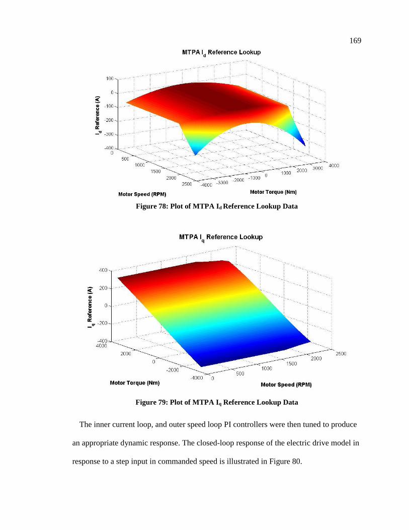
169

Figure 78: Plot of MTPA Id Reference Lookup Data

Figure 79: Plot of MTPA Iq Reference Lookup Data

The inner current loop, and outer speed loop PI controllers were then tuned to produce

an appropriate dynamic response. The closed-loop response of the electric drive model in

response to a step input in commanded speed is illustrated in Figure 80.

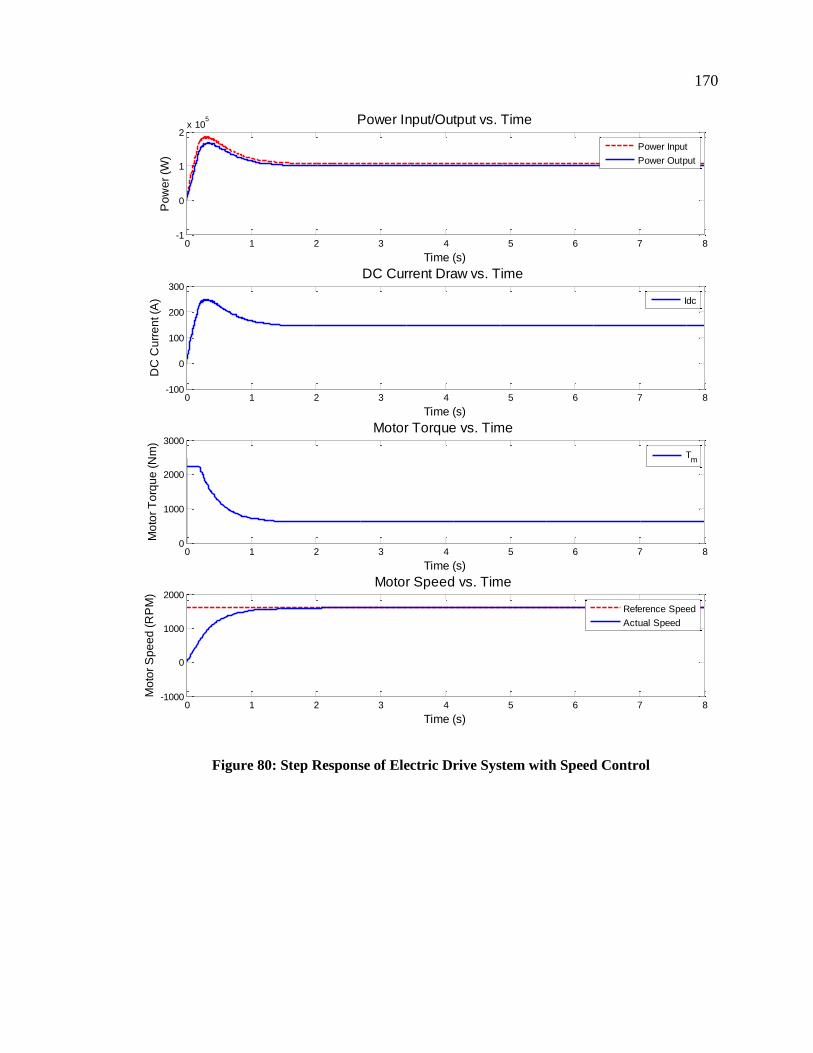
170

Figure 80: Step Response of Electric Drive System with Speed Control

0 1 2 3 4 5 6 7 8-1

0

1

2x 10

5

Time (s)

Po

we

r (W

)

Power Input/Output vs. Time

Power Input

Power Output

0 1 2 3 4 5 6 7 8-100

0

100

200

300

Time (s)

DC

Cu

rre

nt (A

)

DC Current Draw vs. Time

Idc

0 1 2 3 4 5 6 7 80

1000

2000

3000

Time (s)

Mo

tor

To

rqu

e (

Nm

)

Motor Torque vs. Time

Tm

0 1 2 3 4 5 6 7 8-1000

0

1000

2000

Time (s)

Mo

tor

Sp

ee

d (

RP

M)

Motor Speed vs. Time

Reference Speed

Actual Speed

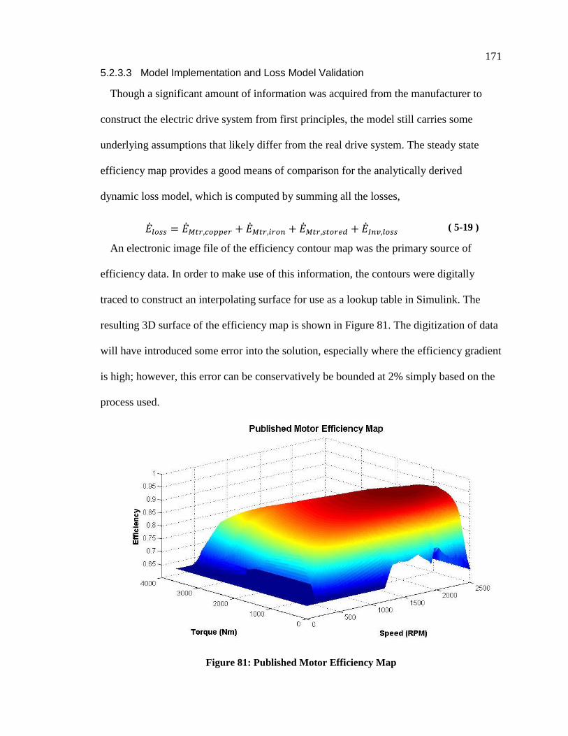
171

5.2.3.3 Model Implementation and Loss Model Validation

Though a significant amount of information was acquired from the manufacturer to

construct the electric drive system from first principles, the model still carries some

underlying assumptions that likely differ from the real drive system. The steady state

efficiency map provides a good means of comparison for the analytically derived

dynamic loss model, which is computed by summing all the losses,

𝑙𝑜𝑠𝑠 = 𝑀𝑡𝑟,𝑐𝑜𝑝𝑝𝑒𝑟 + 𝑀𝑡𝑟,𝑖𝑟𝑜𝑛 + 𝑀𝑡𝑟,𝑠𝑡𝑜𝑟𝑒𝑑 + 𝐼𝑛𝑣,𝑙𝑜𝑠𝑠 ( 5-19 )

An electronic image file of the efficiency contour map was the primary source of

efficiency data. In order to make use of this information, the contours were digitally

traced to construct an interpolating surface for use as a lookup table in Simulink. The

resulting 3D surface of the efficiency map is shown in Figure 81. The digitization of data

will have introduced some error into the solution, especially where the efficiency gradient

is high; however, this error can be conservatively be bounded at 2% simply based on the

process used.

Figure 81: Published Motor Efficiency Map

172

The electric drive system model including the MTPA-based speed controller was

implemented in Simulink such that simulations could be executed programmatically with

an automated test script. The total energy loss is computed using Equation ( 5-19 ).

A steady state comparison between the published drive efficiency and the analytical

loss model is presented in Figure 82. This plot recreates the efficiency contour map, and

overlays the results from each test point denoted with an asterix. The different colours

represent varying degrees of accuracy as described by the legend. Even with the large

number assumptions, it can be seen that the loss model based on first principles provides

reasonable results for high level studies if detailed information is not available. Some

significant discrepancies do occur, primarily in areas exhibiting a high gradient. The

model is also observed to be quite accurate in the high efficiency range of the motor.

The main motivation for implementing a dynamic loss model was to capture the

aggregate transient losses that may not be well represented by a steady state loss model.

Though the first principles model will likely provide a better estimate for transient losses,

it will be seen in Chapter 6 that the load cycles have long stretches during transit where

the operating point is quasi-static. Therefore, the published efficiency data is probably

more suitable for assessing overall energy consumption. As such, the implementation of

the electric drive model allows for two model options, one using steady state data, and

the other with the analytical loss model based on first principles.

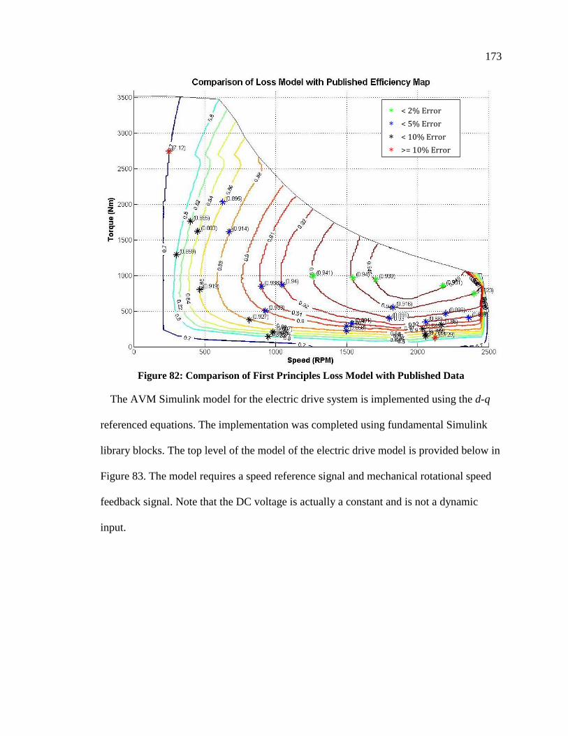
173

Figure 82: Comparison of First Principles Loss Model with Published Data

The AVM Simulink model for the electric drive system is implemented using the d-q

referenced equations. The implementation was completed using fundamental Simulink

library blocks. The top level of the model of the electric drive model is provided below in

Figure 83. The model requires a speed reference signal and mechanical rotational speed

feedback signal. Note that the DC voltage is actually a constant and is not a dynamic

input.

∗ < 2% Error

∗ < 5% Error

∗ < 10% Error

∗ >= 10% Error

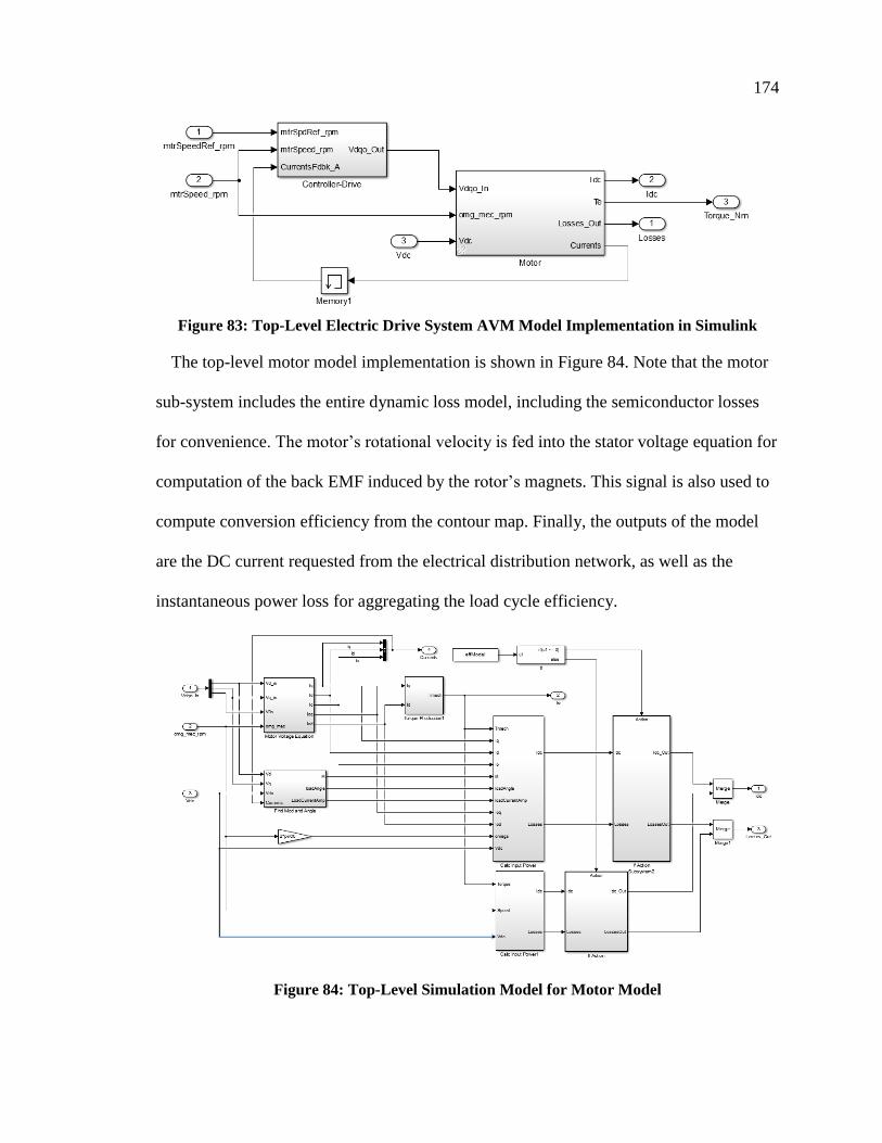
174

Figure 83: Top-Level Electric Drive System AVM Model Implementation in Simulink

The top-level motor model implementation is shown in Figure 84. Note that the motor

sub-system includes the entire dynamic loss model, including the semiconductor losses

for convenience. The motor’s rotational velocity is fed into the stator voltage equation for

computation of the back EMF induced by the rotor’s magnets. This signal is also used to

compute conversion efficiency from the contour map. Finally, the outputs of the model

are the DC current requested from the electrical distribution network, as well as the

instantaneous power loss for aggregating the load cycle efficiency.

Figure 84: Top-Level Simulation Model for Motor Model

175

5.2.3.4 Comparison of AVM to Detailed Simulation Model

In order to validate the AVM developed, a detailed simulation model was also created

in SimPowerSystems to resolve the switching behaviour of the inverter/motor system.

The SVPWM block was used to generate the gate timing signals, while the drive was

assembled using IGBT blocks configured into three separate bridge circuits to represent

the 9-phase output of the electric drive system. The PMSM Simscape motor block only

allows for a three-phase input; therefore, three motor blocks were used to represent the

torque production from all nine phases, and the rotationally conserving ports were

connected together such that the net torque output was summed from each motor block.

The controller developed for the AVM was used directly in the detailed model for

validation; however, the PID controllers were transformed into discrete time. The AVM

and detailed model were then co-simulated with the same step inputs for direct

comparison. Starting from rest initially, Figure 85 shows a comparison between both

models when a step input of 1000rpm is commanded.

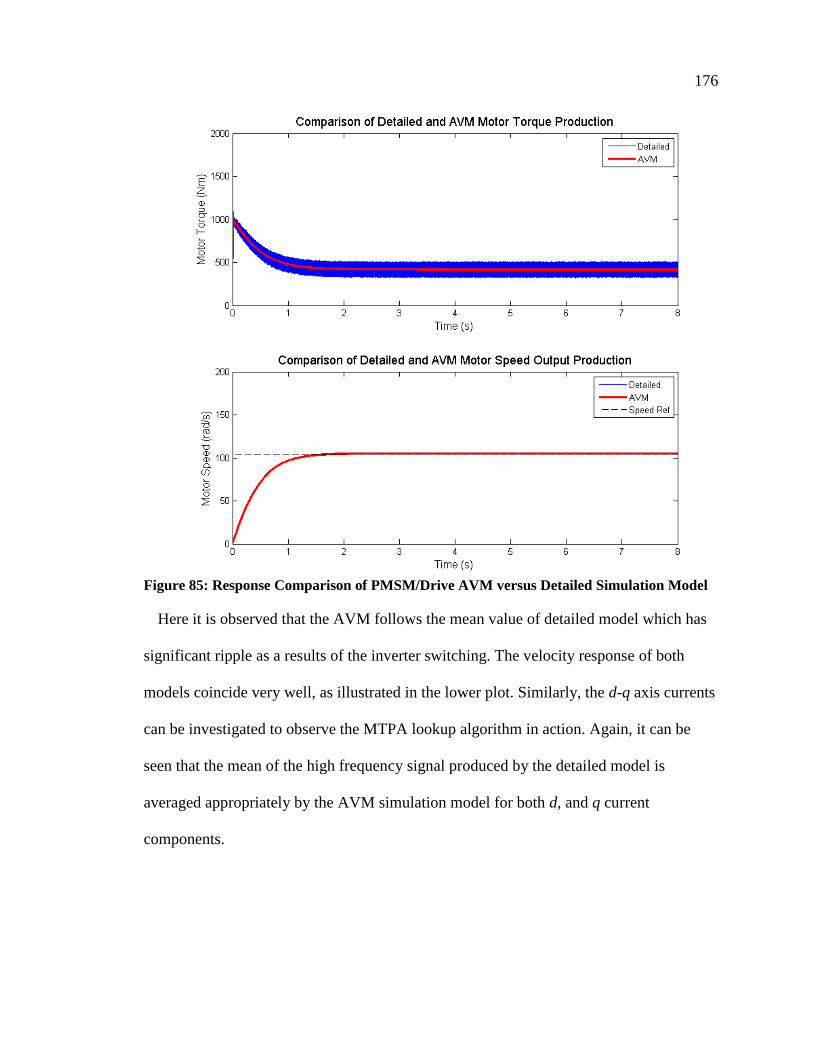
176

Figure 85: Response Comparison of PMSM/Drive AVM versus Detailed Simulation Model

Here it is observed that the AVM follows the mean value of detailed model which has

significant ripple as a results of the inverter switching. The velocity response of both

models coincide very well, as illustrated in the lower plot. Similarly, the d-q axis currents

can be investigated to observe the MTPA lookup algorithm in action. Again, it can be

seen that the mean of the high frequency signal produced by the detailed model is

averaged appropriately by the AVM simulation model for both d, and q current

components.

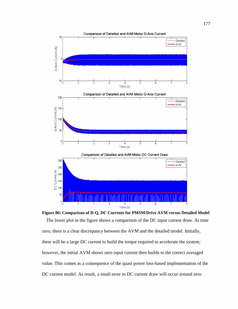
177

Figure 86: Comparison of D-Q, DC Currents for PMSM/Drive AVM versus Detailed Model

The lower plot in the figure shows a comparison of the DC input current draw. At time

zero, there is a clear discrepancy between the AVM and the detailed model. Initially,

there will be a large DC current to build the torque required to accelerate the system;

however, the initial AVM shows zero input current then builds to the correct averaged

value. This comes as a consequence of the quasi power loss-based implementation of the

DC current model. As result, a small error in DC current draw will occur around zero

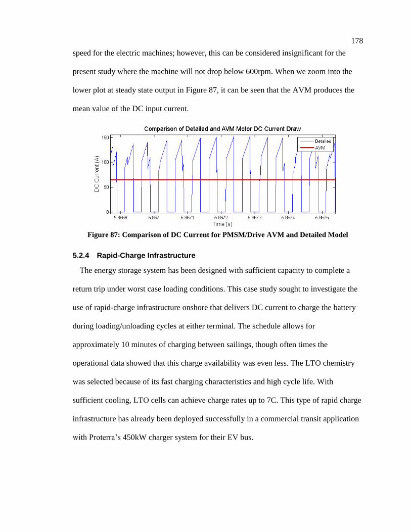
178

speed for the electric machines; however, this can be considered insignificant for the

present study where the machine will not drop below 600rpm. When we zoom into the

lower plot at steady state output in Figure 87, it can be seen that the AVM produces the

mean value of the DC input current.

Figure 87: Comparison of DC Current for PMSM/Drive AVM and Detailed Model

5.2.4 Rapid-Charge Infrastructure

The energy storage system has been designed with sufficient capacity to complete a

return trip under worst case loading conditions. This case study sought to investigate the

use of rapid-charge infrastructure onshore that delivers DC current to charge the battery

during loading/unloading cycles at either terminal. The schedule allows for

approximately 10 minutes of charging between sailings, though often times the

operational data showed that this charge availability was even less. The LTO chemistry

was selected because of its fast charging characteristics and high cycle life. With

sufficient cooling, LTO cells can achieve charge rates up to 7C. This type of rapid charge

infrastructure has already been deployed successfully in a commercial transit application

with Proterra’s 450kW charger system for their EV bus.

179

Lithium batteries are charged using a constant current – constant voltage (CC-CV)

charge profile. The battery management system, vehicle supervisor controller, and charge

controller communicate using standard protocols to regulate the charge process to ensure

that the maximum voltage and current ratings of the battery are not exceeded. If we recall

from Chapter 2, charging begins at a constant current and the cell voltage gradually

climbs until the maximum allowable voltage is achieved. The charger then switches to

maintain constant voltage, then the amount of current drawn by the battery reduces

exponentially until the system is fully charged. Rapid-charge systems are often designed

to execute the CC portion of the charge then disconnect when the maximum voltage is

achieved.

The model must provide the functionality for both CC and CV operation. The capacity

requirements for the onshore charging system for single-ended charging is given below in

Table 29.

Table 29: Charging System Capacity Sizing

Charging System Capacity

Available Charge Time 0.17 h

Desired Charge Rate 5.00 C

Desired Charge Rate (A) 5000.00 ADC

Voltage @ Cutoff 630.00 VDC

Energy Delivered 833.33 Ah

Energy Delivered (kWh) 460.00 kWh

Capacity Percentage 83.3% %

DC Charger Power Output 2.76 MW

While the charging system is connected to the ship, the shore power provides both the

constant battery charge current in addition to the hotel and propulsion demand; therefore,

two PI controllers are required to maintain the CC-CV charge processes. The charger

system implementation is illustrated in Figure 88. The charge logic is governed using a

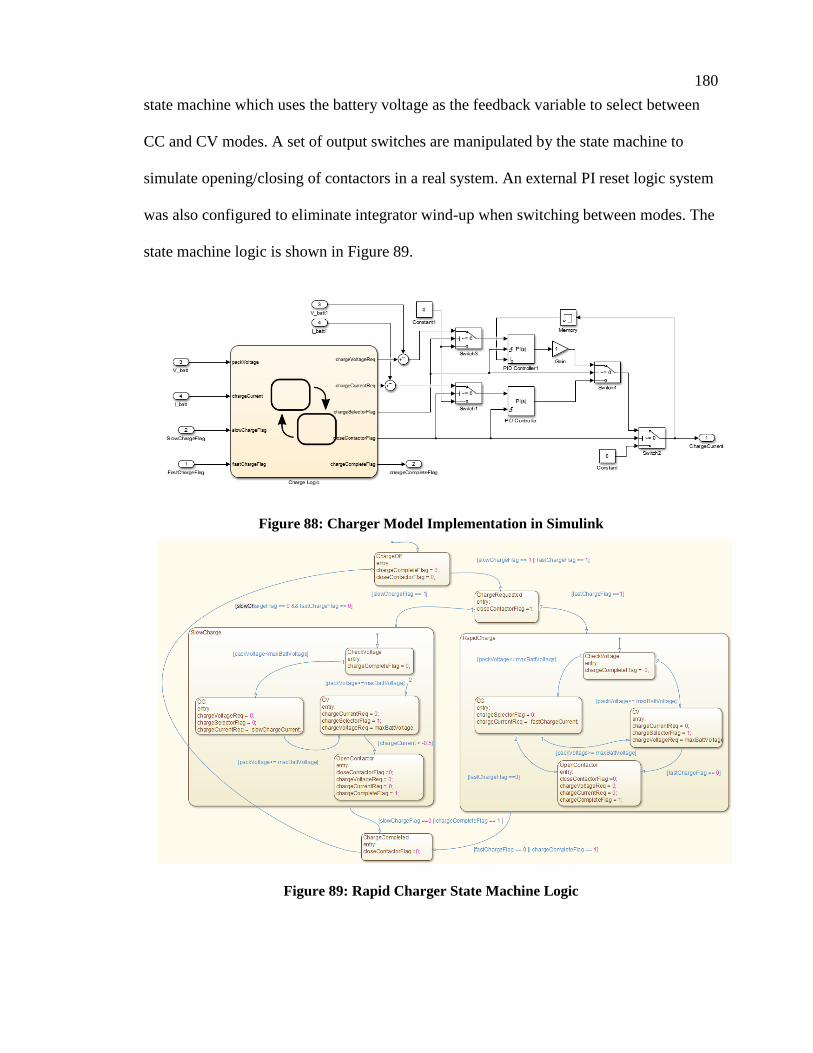
180

state machine which uses the battery voltage as the feedback variable to select between

CC and CV modes. A set of output switches are manipulated by the state machine to

simulate opening/closing of contactors in a real system. An external PI reset logic system

was also configured to eliminate integrator wind-up when switching between modes. The

state machine logic is shown in Figure 89.

Figure 88: Charger Model Implementation in Simulink

Figure 89: Rapid Charger State Machine Logic

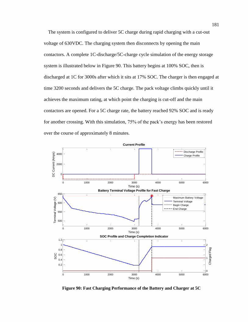
181

The system is configured to deliver 5C charge during rapid charging with a cut-out

voltage of 630VDC. The charging system then disconnects by opening the main

contactors. A complete 1C-discharge/5C-charge cycle simulation of the energy storage

system is illustrated below in Figure 90. This battery begins at 100% SOC, then is

discharged at 1C for 3000s after which it sits at 17% SOC. The charger is then engaged at

time 3200 seconds and delivers the 5C charge. The pack voltage climbs quickly until it

achieves the maximum rating, at which point the charging is cut-off and the main

contactors are opened. For a 5C charge rate, the battery reached 92% SOC and is ready

for another crossing. With this simulation, 75% of the pack’s energy has been restored

over the course of approximately 8 minutes.

Figure 90: Fast Charging Performance of the Battery and Charger at 5C

0 1000 2000 3000 4000 5000 6000

0

2000

4000

Time (s)

DC

Curr

ent (A

mps)

Current Profile

Discharge Profile

Charge Profile

0 1000 2000 3000 4000 5000 6000

500

550

600

650

Time (s)

Term

inal V

olta

ge (

V)

Battery Terminal Voltage Profile for Fast Charge

Maximum Battery Voltage

Terminal Voltage

Begin Charge

End Charge

0 1000 2000 3000 4000 5000 6000

0.2

0.4

0.6

0.8

1

1.2

Time (s)

SO

C

SOC Profile and Charge Completion Indicator

0

1

2

Charg

ed F

lag

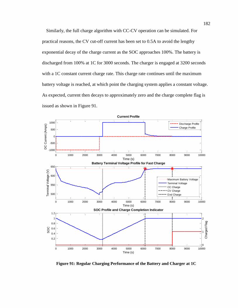
182

Similarly, the full charge algorithm with CC-CV operation can be simulated. For

practical reasons, the CV cut-off current has been set to 0.5A to avoid the lengthy

exponential decay of the charge current as the SOC approaches 100%. The battery is

discharged from 100% at 1C for 3000 seconds. The charger is engaged at 3200 seconds

with a 1C constant current charge rate. This charge rate continues until the maximum

battery voltage is reached, at which point the charging system applies a constant voltage.

As expected, current then decays to approximately zero and the charge complete flag is

issued as shown in Figure 91.

Figure 91: Regular Charging Performance of the Battery and Charger at 1C

0 1000 2000 3000 4000 5000 6000 7000 8000 9000 10000

-1000

-500

0

500

1000

Time (s)

DC

Curr

ent (A

mps)

Current Profile

Discharge Profile

Charge Profile

0 1000 2000 3000 4000 5000 6000 7000 8000 9000 10000

500

550

600

650

Time (s)

Term

inal V

olta

ge (

V)

Battery Terminal Voltage Profile for Fast Charge

Maximum Battery Voltage

Terminal Voltage

CC Charge

CV Charge

End Charge

0 1000 2000 3000 4000 5000 6000 7000 8000 9000 10000

0.2

0.4

0.6

0.8

1

1.2

Time (s)

SO

C

SOC Profile and Charge Completion Indicator

0

1

2

Charg

ed F

lag

183

5.2.5 Islanding Converter for Hotel Loads

In the modern DC grid shipboard integrated power system, islanding converters are

often used to service the AC hotel loads of the ship. One of the major benefits of the DC

grid is its enabling of variable-speed generation for increased conversion efficiency from

the fuel source to electrical energy. The wild AC output of the machine cannot be used

directly for servicing hotel loads because the frequency is unregulated. Hotel loads

require a fixed 50/60Hz signal; consequently, DC/AC islanding converters coupled with

heavy sine filters were designed to provide the sinusoidal AC voltage source for servicing

hotel loads in AES ships equipped with a DC grid. They are referred to as islanding

converters because they are capable of driving the AC grid system without the need to

synchronize to a voltage waveform.

The detailed topology, analysis, and control of this type of converter is well beyond the

scope of this document; however, a model is required to account for electrical load

demand on the M.V. Klitsa. The hotel loads for this ship are an order of magnitude less

than the propulsive loads, and won’t be dominant. As a first approximation, the converter

will be assumed to have a constant conversion efficiency of 93% as is typical in

converters in the 50kW range. This power loss model will compute the distribution side

DC current demand using the hotel load profile collected in the data acquisition study.

The model of the converter approximation is shown below in Figure 92.

Figure 92: DC/AC Converter Approximation Model Implementation

184

Chapter 6 Summary of M.V. Klitsa Data Acquisition Experiment

and Load Profile Generation

6.1 Introduction to Data Acquisition Experiment

One of the key factors to designing an effective hybrid propulsion systems lies in

having a priori knowledge of the ship’s expected operational profiles. With advanced

knowledge of the mission cycles and their statistical distribution, the system can be

optimized to deliver the best possible performance while minimizing energy

consumption. The MIL platform under development seeks to provide a predictive tool for

extracting the load profile based on defined mission cycles. When real operational data is

available, it can also facilitate with more detailed design, validation analysis, and control

system development.

The short-cross ferry application was selected as the case study partially because of its

consistent, and well-defined operating profile. In order to validate the integrated time-

domain modeling framework, it was imperative to obtain operational data for the Klitsa

as a means of direct comparison. The data acquisition study provided insight into the

expected propulsive and hotel load variation, and, as will be seen in this chapter, has also

enabled the creation of standardized load cases the can be used as metrics for evaluating

different architectures.

Though the ship has been upgraded to include a monitoring and control system, the

individual signals to be acquired were not conveniently accessed on a single

communication bus; consequently, an independent CAN communication network was

installed onboard the ship to enable a single collection point for all signals with time-

synchronization. Separate sensors and instrumentation were installed for systems that did

not offer a convenient signal source. The full design of the experiment and installation

185

details are provided in Appendix A. In this chapter, we will limit the discussion to the key

features of, and results produced by, the data acquisition study. The master signal list,

along with the signal source is summarized in Table 30.

Table 30: Summary of Acquired Parameters in Data Acquisition Study

Description Physical Parameter Transducer Signal Source

GPS Data Position (NED) Cross Chasm GPS Logger

Vessel Speed Cross Chasm GPS Logger

Engine 1 Data

Engine Load J1587/J1708 Serial Bus

Engine Speed J1587/J1708 Serial Bus

Engine Torque J1587/J1708 Serial Bus

Throttle Demand J1587/J1708 Serial Bus

Engine 2 Data

Engine Load J1587/J1708 Serial Bus




Azimuth Propeller 1 Azimuth Angle Position HRP NMEA0183 Serial Bus

Thruster Position Reference HRP NMEA0183 Serial Bus

Azimuth Propeller 2 Azimuth Angle Position HRP NMEA0183 Serial Bus

Thruster Position Reference HRP NMEA0183 Serial Bus

Generator Output 3-Phase Power Veris H8043-0300-2 Power Sensor

Wind Data Wind Speed Campbell Scientific 05103LK Wind Monitor

Direction Campbell Scientific 05103LK Wind Monitor

Heading/Attitude

Heading Direction Maretron SSC200 Fluxgate Gyrocompass

Pitch Angle Maretron SSC200 Fluxgate Gyrocompass

Roll Angle Maretron SSC200 Fluxgate Gyrocompass

Turn Rate Maretron SSC200 Fluxgate Gyrocompass

The data acquisition system made use of the onboard J1587/J1708 serial

communication bus for the engines, and the NMEA183 serial bus from the azimuth angle

thruster systems. Custom serial converters were developed to read from the onboard

serial buses to broadcast the data over the CAN network. CAN traffic was logged using

the Cross-Chasm data logger, which also contains an integrated GPS system that was

used for tracking vessel position and speed. The system was designed to operate

autonomously using an enable message to trigger all nodes to begin broadcasting. The

enable was trigger by sensing Engine 1’s serial communication bus activity. A schematic

of the instrumentation and communication network layout is provided in Figure 93.

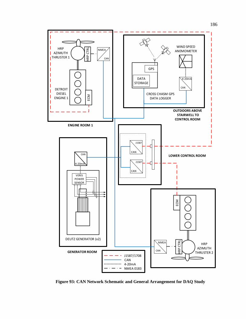
186

VERISPOWER SENSOR

DEUTZ GENERATOR (x2)

J1587

CAN

GPS

DATA STORAGE

CAN

4-20mA

CROSS CHASM GPSDATA LOGGER

HR

P CT

RL

WIND SPEEDANEMOMETER

DETROIT DIESEL

ENGINE 1

EC

M

ECM

LOWER CONTROL ROOM

HRP AZIMUTH

THRUSTER 1

HRP AZIMUTH

THRUSTER 2J1587/1708CAN4-20mANMEA 0183

HR

P C

TRL

CAN

NMEA

J1587

CAN

CAN

4-20mA

ENGINE ROOM 1

OUTDOORS ABOVE STAIRWELL TO

CONTROL ROOM

GENERATOR ROOM CAN

NMEA

Figure 93: CAN Network Schematic and General Arrangement for DAQ Study

187

6.2 Development of Load Profiles from Operational Data

Approximately two months’ worth of data was collected onboard the ship; however,

many technical issues arose with various components which often led to incomplete data.

The engine signals were consistently noisy and the system was pulled offline several

times in attempt to resolve the issue. The original installation seemed to provide the

cleanest signals, and were therefore used in the development of the standard load profiles.

The Cross Chasm GPS logger was also found to have a manufacturers’ defect in the

firmware which would randomly scale the velocity of the ship to the point where the

signal was no longer usable.

Despite these problems, several well-conditioned and complete datasets were extracted

and developed into a set of representative load profiles of differing power outputs. The

primary parameters required for validation of the model are as follows:

1. Propulsion System Load: Torque/Speed vs. Time

2. Hotel Loads: Electrical Power vs. Time

3. Propeller Position: Azimuth Angle vs. Time

4. Vessel Speed vs. Time

The two main diesel engines and the auxiliary generator supply all of the energy

required for the ship, and are thus the most important for computing energy demands for

the BEIPS. The load information from the engines was captured from the ECM units,

which are not-known to have very high precision. The measured engine load can be

compared against the published propeller data in the first quadrant as a sanity check. The

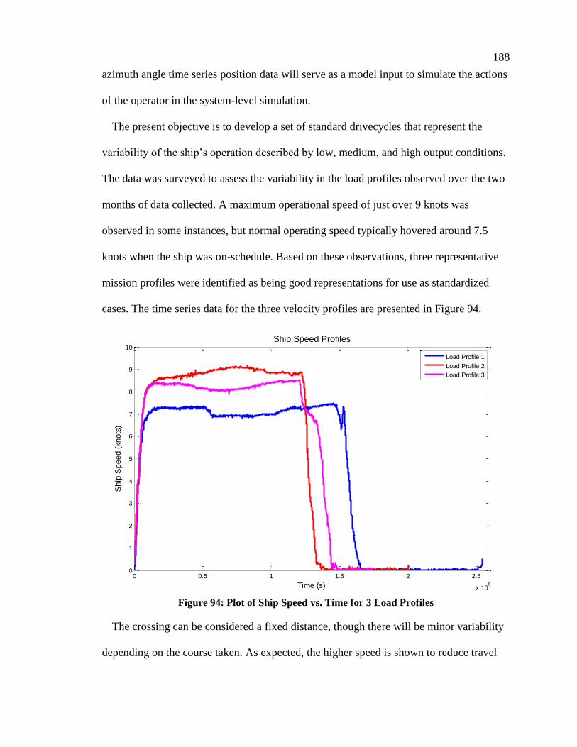
188

azimuth angle time series position data will serve as a model input to simulate the actions

of the operator in the system-level simulation.

The present objective is to develop a set of standard drivecycles that represent the

variability of the ship’s operation described by low, medium, and high output conditions.

The data was surveyed to assess the variability in the load profiles observed over the two

months of data collected. A maximum operational speed of just over 9 knots was

observed in some instances, but normal operating speed typically hovered around 7.5

knots when the ship was on-schedule. Based on these observations, three representative

mission profiles were identified as being good representations for use as standardized

cases. The time series data for the three velocity profiles are presented in Figure 94.

Figure 94: Plot of Ship Speed vs. Time for 3 Load Profiles

The crossing can be considered a fixed distance, though there will be minor variability

depending on the course taken. As expected, the higher speed is shown to reduce travel

0 0.5 1 1.5 2 2.5

x 106

0

1

2

3

4

5

6

7

8

9

10

Time (s)

Sh

ip S

pe

ed

(kn

ots

)

Ship Speed Profiles

Load Profile 1

Load Profile 2

Load Profile 3

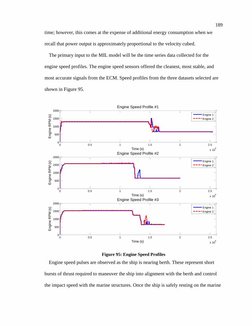
189

time; however, this comes at the expense of additional energy consumption when we

recall that power output is approximately proportional to the velocity cubed.

The primary input to the MIL model will be the time series data collected for the

engine speed profiles. The engine speed sensors offered the cleanest, most stable, and

most accurate signals from the ECM. Speed profiles from the three datasets selected are

shown in Figure 95.

Figure 95: Engine Speed Profiles

Engine speed pulses are observed as the ship is nearing berth. These represent short

bursts of thrust required to maneuver the ship into alignment with the berth and control

the impact speed with the marine structures. Once the ship is safely resting on the marine

0 0.5 1 1.5 2 2.5

x 106

0

500

1000

1500

2000

Time (s)

En

gin

e R

PM

(s)

Engine Speed Profile #1

Engine 1

Engine 2

0 0.5 1 1.5 2 2.5

x 106

0

500

1000

1500

2000

Time (s)

En

gin

e R

PM

(s)


Engine 1

Engine 2

0 0.5 1 1.5 2 2.5

x 106

0

500

1000

1500

2000

Time (s)

En

gin

e R

PM

(s)


Engine 1

Engine 2

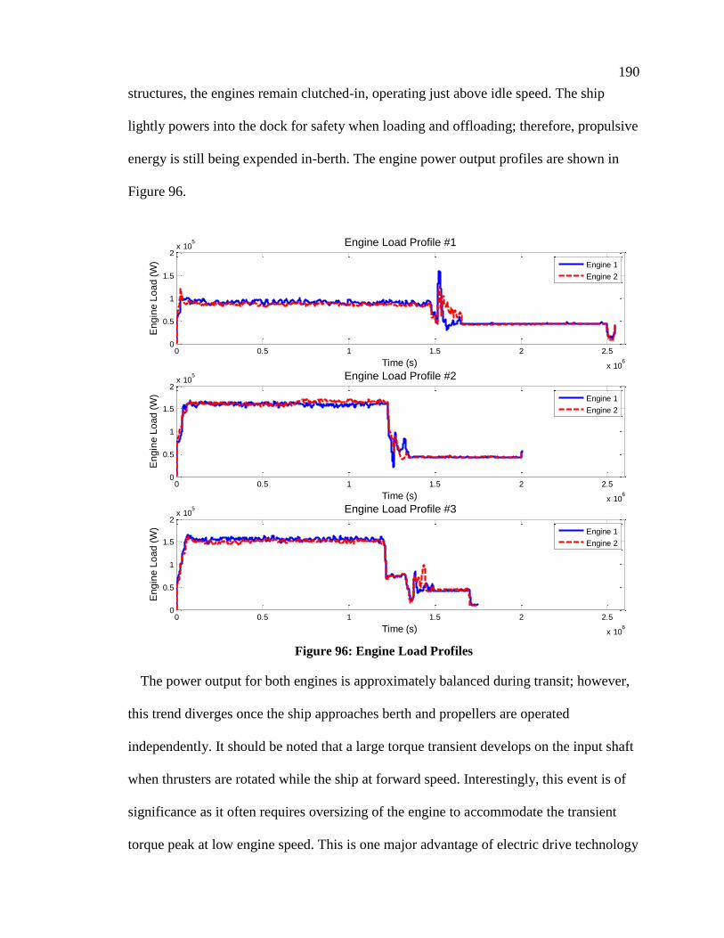
190

structures, the engines remain clutched-in, operating just above idle speed. The ship

lightly powers into the dock for safety when loading and offloading; therefore, propulsive

energy is still being expended in-berth. The engine power output profiles are shown in

Figure 96.

Figure 96: Engine Load Profiles

The power output for both engines is approximately balanced during transit; however,

this trend diverges once the ship approaches berth and propellers are operated

independently. It should be noted that a large torque transient develops on the input shaft

when thrusters are rotated while the ship at forward speed. Interestingly, this event is of

significance as it often requires oversizing of the engine to accommodate the transient

torque peak at low engine speed. This is one major advantage of electric drive technology

0 0.5 1 1.5 2 2.5

x 106

0

0.5

1

1.5

2x 10

5

Time (s)

En

gin

e L

oa

d (

W)

Engine Load Profile #1

Engine 1

Engine 2

0 0.5 1 1.5 2 2.5

x 106

0

0.5

1

1.5

2x 10

5

Time (s)

En

gin

e L

oa

d (

W)


Engine 1

Engine 2

0 0.5 1 1.5 2 2.5

x 106

0

0.5

1

1.5

2x 10

5

Time (s)

En

gin

e L

oa

d (

W)


Engine 1

Engine 2

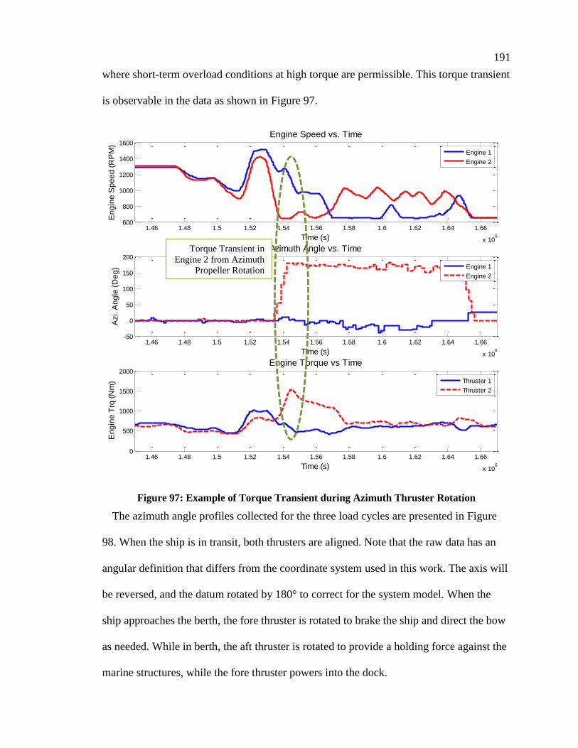
191

where short-term overload conditions at high torque are permissible. This torque transient

is observable in the data as shown in Figure 97.

Figure 97: Example of Torque Transient during Azimuth Thruster Rotation

The azimuth angle profiles collected for the three load cycles are presented in Figure

98. When the ship is in transit, both thrusters are aligned. Note that the raw data has an

angular definition that differs from the coordinate system used in this work. The axis will

be reversed, and the datum rotated by 180° to correct for the system model. When the

ship approaches the berth, the fore thruster is rotated to brake the ship and direct the bow

as needed. While in berth, the aft thruster is rotated to provide a holding force against the

marine structures, while the fore thruster powers into the dock.

1.46 1.48 1.5 1.52 1.54 1.56 1.58 1.6 1.62 1.64 1.66

x 106

600

800

1000

1200

1400

1600

Time (s)

En

gin

e S

pe

ed

(R

PM

)

Engine Speed vs. Time

Engine 1

Engine 2

1.46 1.48 1.5 1.52 1.54 1.56 1.58 1.6 1.62 1.64 1.66

x 106

-50

0

50

100

150

200

Time (s)

Azi. A

ng

le (

De

g)

Azimuth Angle vs. Time

Engine 1

Engine 2

1.46 1.48 1.5 1.52 1.54 1.56 1.58 1.6 1.62 1.64 1.66

x 106

0

500

1000

1500

2000

Time (s)

En

gin

e T

rq (

Nm

)

Engine Torque vs Time

Thruster 1

Thruster 2

Torque Transient in

Engine 2 from Azimuth

Propeller Rotation

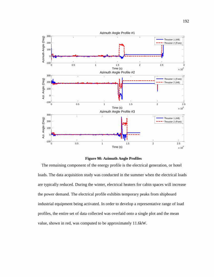
192

Figure 98: Azimuth Angle Profiles

The remaining component of the energy profile is the electrical generation, or hotel

loads. The data acquisition study was conducted in the summer when the electrical loads

are typically reduced. During the winter, electrical heaters for cabin spaces will increase

the power demand. The electrical profile exhibits temporary peaks from shipboard

industrial equipment being activated. In order to develop a representative range of load

profiles, the entire set of data collected was overlaid onto a single plot and the mean

value, shown in red, was computed to be approximately 11.6kW.

0 0.5 1 1.5 2 2.5 3

x 106

-100

0

100

200

300

Time (s)

Azim

uth

An

gle

(D

eg

)

Azimuth Angle Profile #1

Thruster 1 (Aft)

Thruster 2 (Fore)

0 0.5 1 1.5 2 2.5

x 106

-100

0

100

200

300

Time (s)

Azi. A

ng

le (

De

g)


Thruster 1 (Fore)

Thruster 2 (Aft)

0 0.5 1 1.5 2 2.5

x 106

-100

0

100

200

300

Time (s)

Azi. A

ng

le (

De

g)


Thruster 1 (Aft)

Thruster 2 (Fore)

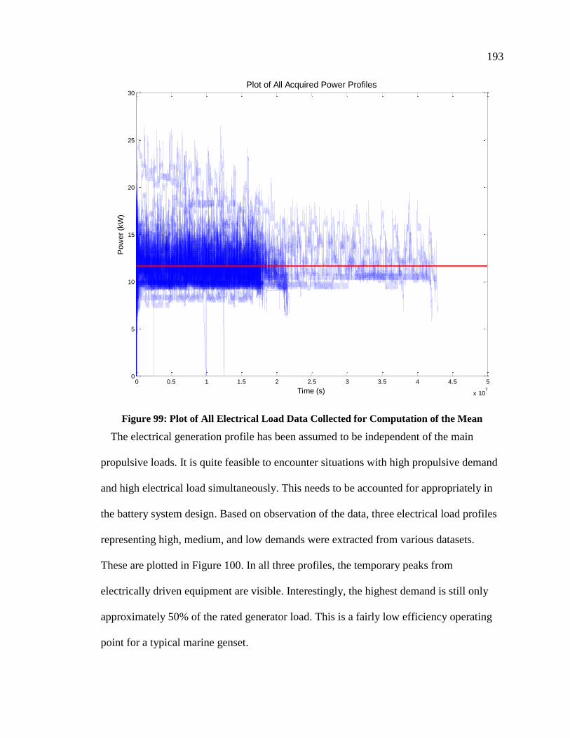
193

Figure 99: Plot of All Electrical Load Data Collected for Computation of the Mean

The electrical generation profile has been assumed to be independent of the main

propulsive loads. It is quite feasible to encounter situations with high propulsive demand

and high electrical load simultaneously. This needs to be accounted for appropriately in

the battery system design. Based on observation of the data, three electrical load profiles

representing high, medium, and low demands were extracted from various datasets.

These are plotted in Figure 100. In all three profiles, the temporary peaks from

electrically driven equipment are visible. Interestingly, the highest demand is still only

approximately 50% of the rated generator load. This is a fairly low efficiency operating

point for a typical marine genset.

0 0.5 1 1.5 2 2.5 3 3.5 4 4.5 5

x 107

0

5

10

15

20

25

30

Time (s)

Po

we

r (k

W)

Plot of All Acquired Power Profiles

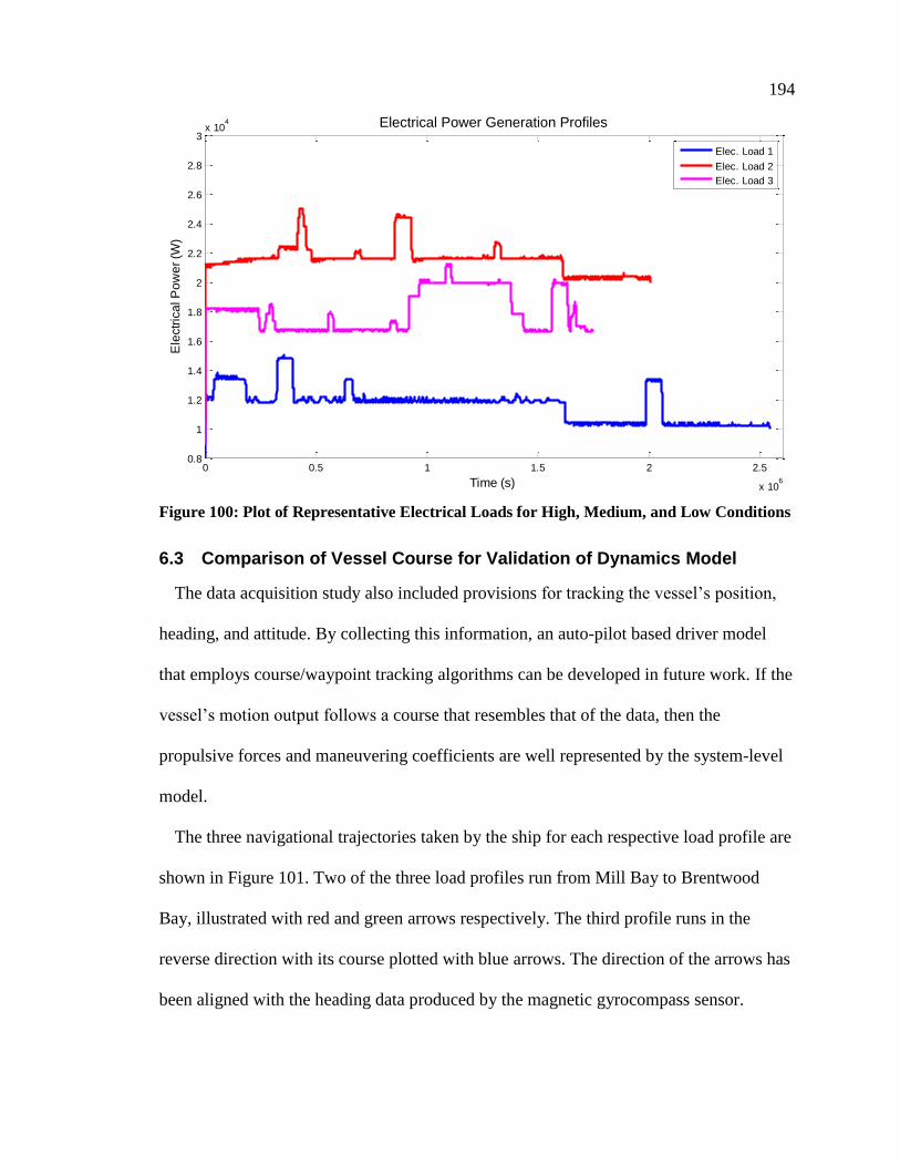
194

Figure 100: Plot of Representative Electrical Loads for High, Medium, and Low Conditions

6.3 Comparison of Vessel Course for Validation of Dynamics Model

The data acquisition study also included provisions for tracking the vessel’s position,

heading, and attitude. By collecting this information, an auto-pilot based driver model

that employs course/waypoint tracking algorithms can be developed in future work. If the

vessel’s motion output follows a course that resembles that of the data, then the

propulsive forces and maneuvering coefficients are well represented by the system-level

model.

The three navigational trajectories taken by the ship for each respective load profile are

shown in Figure 101. Two of the three load profiles run from Mill Bay to Brentwood

Bay, illustrated with red and green arrows respectively. The third profile runs in the

reverse direction with its course plotted with blue arrows. The direction of the arrows has

been aligned with the heading data produced by the magnetic gyrocompass sensor.

0 0.5 1 1.5 2 2.5

x 106

0.8

1

1.2

1.4

1.6

1.8

2

2.2

2.4

2.6

2.8

3x 10

4

Time (s)

Ele

ctr

ica

l P

ow

er

(W)

Electrical Power Generation Profiles

Elec. Load 1

Elec. Load 2

Elec. Load 3

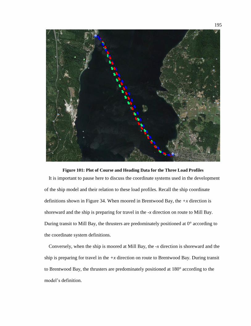
195

Figure 101: Plot of Course and Heading Data for the Three Load Profiles

It is important to pause here to discuss the coordinate systems used in the development

of the ship model and their relation to these load profiles. Recall the ship coordinate

definitions shown in Figure 34. When moored in Brentwood Bay, the +x direction is

shoreward and the ship is preparing for travel in the -x direction on route to Mill Bay.

During transit to Mill Bay, the thrusters are predominately positioned at 0° according to

the coordinate system definitions.

Conversely, when the ship is moored at Mill Bay, the -x direction is shoreward and the

ship is preparing for travel in the +x direction on route to Brentwood Bay. During transit

to Brentwood Bay, the thrusters are predominately positioned at 180° according to the

model’s definition.

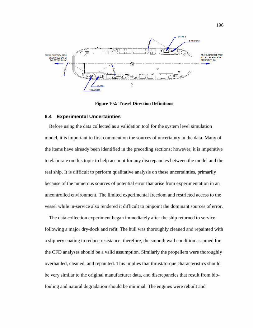
196

Figure 102: Travel Direction Definitions

6.4 Experimental Uncertainties

Before using the data collected as a validation tool for the system level simulation

model, it is important to first comment on the sources of uncertainty in the data. Many of

the items have already been identified in the preceding sections; however, it is imperative

to elaborate on this topic to help account for any discrepancies between the model and the

real ship. It is difficult to perform qualitative analysis on these uncertainties, primarily

because of the numerous sources of potential error that arise from experimentation in an

uncontrolled environment. The limited experimental freedom and restricted access to the

vessel while in-service also rendered it difficult to pinpoint the dominant sources of error.

The data collection experiment began immediately after the ship returned to service

following a major dry-dock and refit. The hull was thoroughly cleaned and repainted with

a slippery coating to reduce resistance; therefore, the smooth wall condition assumed for

the CFD analyses should be a valid assumption. Similarly the propellers were thoroughly

overhauled, cleaned, and repainted. This implies that thrust/torque characteristics should

be very similar to the original manufacturer data, and discrepancies that result from bio-

fouling and natural degradation should be minimal. The engines were rebuilt and

197

dynamometer tested as part of the refit; therefore, the rated output and ECM calibrations

would have been factory reset and verified with the test bench.

With this information, the major sources of experimental error that remain surround the

following items:

1. Environmental conditions

2. ECM measurements and torque computation

3. Hydraulic PTO loading

4. Signal noise in engine data

6.4.1 Environmental Errors

There is clear evidence that environmental factors had some influence on the

performance of the vessel. For example, the spread of the data points observed in section

4.1.5 in formulation of the thrust deduction factor highlights the discrepancies between

similar operating points, mainly engine speed versus vessel speed. This naturally points

to environmental factors which are concurrently influencing the loading of the ship.

Based on the survey of historic wave data in the Saanich Inlet conducted in Chapter 4,

and cross-referencing with the actual weather on the date of the data collected, it is highly

unlikely that wave loading was a dominant factor. This leaves current and wind as the

potential influencing factors.

An anemometer was configured as part of the data collection study. The anemometer

was able to capture relative speed and heading of the wind with respect to the ship.

Because the air resistance coefficient wasn’t analyzed as part of this work, this forcing

factor was not fully accounted for in the analysis. The method by which the load profiles

in section 6.2 were selected was largely based on investigation of the wind profile.

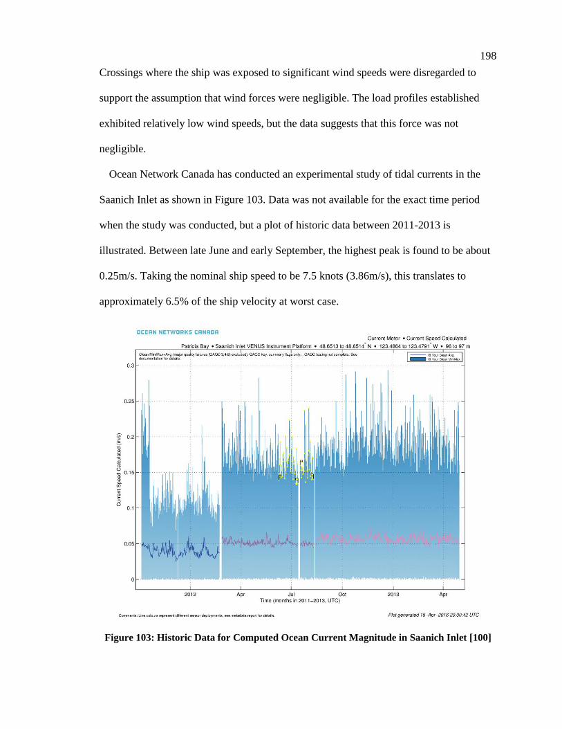
198

Crossings where the ship was exposed to significant wind speeds were disregarded to

support the assumption that wind forces were negligible. The load profiles established

exhibited relatively low wind speeds, but the data suggests that this force was not

negligible.

Ocean Network Canada has conducted an experimental study of tidal currents in the

Saanich Inlet as shown in Figure 103. Data was not available for the exact time period

when the study was conducted, but a plot of historic data between 2011-2013 is

illustrated. Between late June and early September, the highest peak is found to be about

0.25m/s. Taking the nominal ship speed to be 7.5 knots (3.86m/s), this translates to

approximately 6.5% of the ship velocity at worst case.

Figure 103: Historic Data for Computed Ocean Current Magnitude in Saanich Inlet [100]

199

The approximate heading for the measured current about 140° for the May –

September time period. The direction is shown relative to the Brentwood Bay – Mill Bay

crossing in Figure 104. It can be seen that the current direction could have potentially

assisted with the ship in its travel from Mill Bay, and added additional resistance when

traveling from Brentwood Bay.

Figure 104: Approximate Current Heading from Ocean Networks Canada versus

Brentwood Bay – Mill Bay Crossing [101]

200

6.4.2 ECM Measurement Errors

The diesel engine ECM output for engine load is not a direct power measurement, but

rather a computation based on fuel rates, engine speed, and measurements of the air fuel

mixture. If calibrations are correct this signal should provide reasonably accurate results

for power output estimation when the engine is operating at quasi-steady state, likely

within ±5%. However during transient conditions, especially at low loads, the computed

load may diverge from the real value. A literature search was conducted in an attempt to

quantify this error during transient conditions. Unfortunately, the search did not yield

direct any good comparative data between power computation and direct measurement

for similar scale diesel engines.

6.4.3 Signal Noise in Engine Signals

The engine signals were converted from the J1587/1708 onboard engine

communication bus to CAN message through custom-built gateway controllers. The

intermediate signal conversion process from J1587 to RS232 exhibited a significant

amount of high frequency noise and erroneous data that propagated into the dataset.

Multiple filtering techniques were attempted to clean up the signal, but a significant post-

processing effort was required recreate a realistic load profile. Out of range values were

eliminated, and a moving average filter was applied to the data to smooth out erroneous

data points. As a result, the post processed load profiles may have damped out higher

frequency transients during the maneuvering section that may have account for

discrepancies in the model results.

201

Chapter 7 System Model Validation and Simulation Results

The previous chapters have established the mathematical formulation and Simulink

implementation that make-up the BEIPS propulsion architecture, the thruster system, and

the hull performance. In this chapter, these components are assembled into a system-level

model to validate the simulation framework against real-world operational data. The

system-level model allows for component interactions and dependencies to be studied in

greater detail. The behaviour can then be compared against results from the real system.

Though the full 6-DOF equations of motion for the vessel have been implemented in

the vessel dynamics model, the simulations here are constrained to a single DOF that

considers only surge. This simplification was required in this initial body of work

because the asymmetric thruster configuration and skeg forces combine to produce a

numerically unbalanced yaw moment. Without an auto-pilot algorithm with path

tracking, the numerical imbalance caused the ship to turn slightly and go off course.

Development of a control algorithm to manage the azimuthing thrusters in this particular

configuration is a non-trivial task, so this has been left as future work.

Using the 1-DOF assumption, the model can be systematically tested using the

experimental data to validate different sub-systems of the simulation model. The most

significant factor that directly affects the powertrain load is the ship velocity. When the

ship velocity is under-predicted given the same propeller speed, the advance ratio is

decreased thereby increasing propeller torque to produce an over-prediction of energy

consumption. Conversely, over-prediction of velocity will produce an under-prediction of

energy consumption. The thruster model and wake fraction estimator are also sensitive to

changes in velocity. Both of these sub-systems also influence the powertrain load.

202

In order to isolate these sub-systems for validation, the first set of simulations disabled

the vessel dynamics model and imposed the experimental velocity profile collected by the

GPS unit in the DAQ experiment. The model’s performance was then computed by

feeding time series data for engine speed, and azimuth angle data as inputs. This

approach provided a direct means of comparison for the powertrain load predictions

against the engine load data collected from the ECM.

The second set of simulations included the vessel dynamics model to investigate the

full model performance. With the 1-DOF motion constraint, the propeller forces were

limited to the x-direction to consider only forces in the surge sub-system. This set of

simulations assessed the model’s ability to capture dynamic actuation forces for

maneuvering and cruise conditions, and how these actuation forces propagate to the IPS.

Before presenting the simulation results for both test cases, this chapter will begin by

illustrating the system-level model implementation and configuration in Simulink. This is

followed by a presentation of the simulation results, and lastly, a comprehensive

discussion of the results and the level of success achieved using this methodology.

7.1 System Model Implementation

Due to the large number of sub-systems, the model will be presented in sections for

clarity. The overall propulsion system of the model is shown in Figure 105. This model is

divided by two coloured boxes, including an overlap section around the propeller models.

The blue box illustrates the information flow between the electrical power system models

and the propeller models, with further detail shown in Figure 106. The red box illustrates

the actuation forces and the vessel dynamics model, with further detail shown in Figure

107.

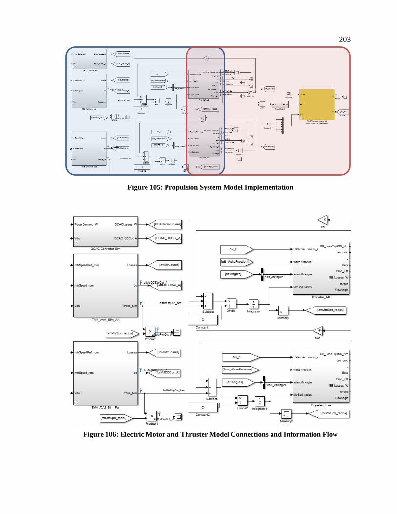
203

Figure 105: Propulsion System Model Implementation

Figure 106: Electric Motor and Thruster Model Connections and Information Flow

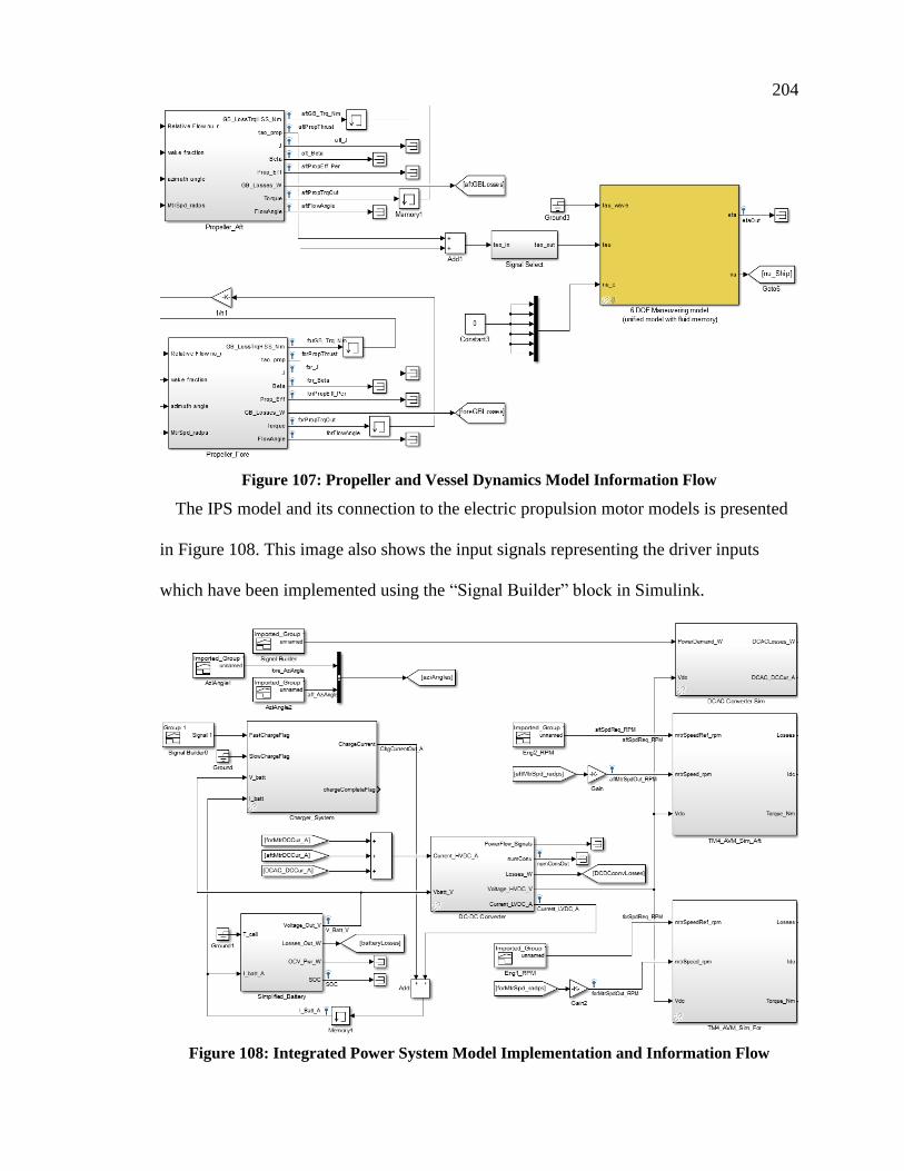
204

Figure 107: Propeller and Vessel Dynamics Model Information Flow

The IPS model and its connection to the electric propulsion motor models is presented

in Figure 108. This image also shows the input signals representing the driver inputs

which have been implemented using the “Signal Builder” block in Simulink.

Figure 108: Integrated Power System Model Implementation and Information Flow

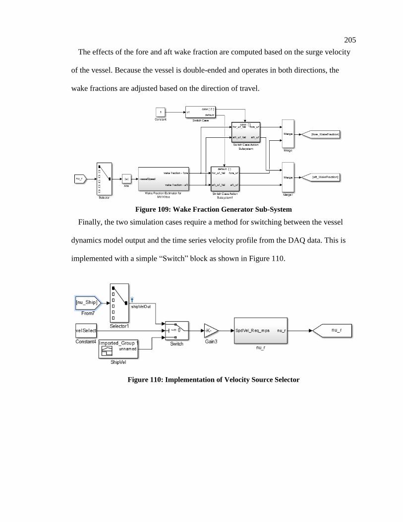
205

The effects of the fore and aft wake fraction are computed based on the surge velocity

of the vessel. Because the vessel is double-ended and operates in both directions, the

wake fractions are adjusted based on the direction of travel.

Figure 109: Wake Fraction Generator Sub-System

Finally, the two simulation cases require a method for switching between the vessel

dynamics model output and the time series velocity profile from the DAQ data. This is

implemented with a simple “Switch” block as shown in Figure 110.

Figure 110: Implementation of Velocity Source Selector

206

7.2 Powertrain Load Prediction and Verification

7.2.1 Simulation Results for Different Load Profiles

The first set of simulations disabled the vessel dynamics model from the analysis, and

instead, applied the experimental velocity data for the three load profiles directly. The

GPS velocity profile data was loaded into a “Signal Builder” block, and the model was

configured to disable the vessel dynamics output as a feedback variable, see Figure 110.

The azimuth angle commanded was also directly specified using experimental data to

assess the thruster model’s effectiveness of capturing transient off-design performance

during maneuvers.

The motor speed time-series data collected in the DAQ experiments was also

configured as a model input; however, this was used as reference signal to the PI speed

controller in the motor drive. The controller was tuned to closely track the signal, thereby

minimizing any engine/motor speed discrepancies between model and data. The

simulation was performed for the three load profiles, and the results are shown in Figure

111 through Figure 113.

Each cycle begins the instant that the ferry pushes back from the dock and ramps up

engines to begin the crossing. The ramp-up period is followed by relatively steady state

operation while in transit. As the ferry approaches its destination, the engines are ramped

down and the vessel is dynamically braked by the driver. Pulses of thrust are delivered to

maneuver the ship into berth and gently touch the marine structures. Once in place, the

ship powers into berth at a constant low power output while vehicles are offloaded and

then subsequently reloaded. The cycle concludes just before the ship pushes back for its

next crossing.

207

The results are generally in good agreement; however, one blatant discrepancy across

all three simulations is the significant under-prediction of propulsive load when the ship

is in berth. The propeller torque produced by the thruster model was confirmed to be

correct when cross-referenced by the manufacturer’s datasheet. It was found that the

hydraulic actuation system for the azimuthing thruster is driven off the output shaft of the

engine as a PTO. The loading is relatively small compared to the rated output of the

engine; however, it is the dominant source of load while in berth.

In addition to the hydraulic system, the right angled gearbox arrangement is not likely

well represented by linear damping alone. Coulomb friction and other factors are likely

present, but experimental characterization of the damping model was not feasible with

the ship in service. The analysis performed by the manufacturer in the original propulsion

system design for the Klitsa assumed a constant 15% loss for the propeller system,

including hydraulic system PTO. This assumption was initially dismissed as being overly

conservative, but the operational data suggests that these systems are reasonably

approximated by a constant damping load combined with a speed-dependent damping

term.

As a simple revision to the damping model, the linear damping torque was numerically

backed out of the simulation results. A revised damping model was numerically inserted

to maintain a constant 28kW of damping load to coincide with experimental observation,

but also accounting for speed dependent linear damping in the gearbox. The new model

was implemented as linear function whose output is fed into a “Saturation” block with

lower limit of 28kW. This value is about 10.7% of rated load, and is well below the

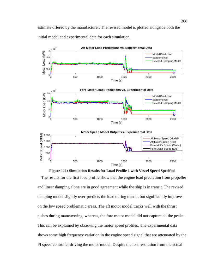
208

estimate offered by the manufacturer. The revised model is plotted alongside both the

initial model and experimental data for each simulation.

Figure 111: Simulation Results for Load Profile 1 with Vessel Speed Specified

The results for the first load profile show that the engine load prediction from propeller

and linear damping alone are in good agreement while the ship is in transit. The revised

damping model slightly over-predicts the load during transit, but significantly improves

on the low speed problematic areas. The aft motor model tracks well with the thrust

pulses during maneuvering, whereas, the fore motor model did not capture all the peaks.

This can be explained by observing the motor speed profiles. The experimental data

shows some high frequency variation in the engine speed signal that are attenuated by the

PI speed controller driving the motor model. Despite the lost resolution from the actual

0 500 1000 1500 2000 25000

0.5

1

1.5

2x 10

5

Time (s)

Mo

tor

Lo

ad

(kW

)

Aft Motor Load Predictions vs. Experimental Data

Model Prediction

Experimental

Revised Damping Model

0 500 1000 1500 2000 25000

5

10

15x 10

4

Time (s)

Mo

tor

Lo

ad

(kW

)

Fore Motor Load Predictions vs. Experimental Data

Model Prediction

Experimental


0 500 1000 1500 2000 25000

500

1000

1500

2000

Time (s)

Mo

tor

Sp

ee

d (

RP

M) Motor Speed Model Output vs. Experimental Data

Aft Motor Speed (Model)

Aft Motor Speed (Exp)

Fore Motor Speed (Model)

Fore Motor Speed (Exp)

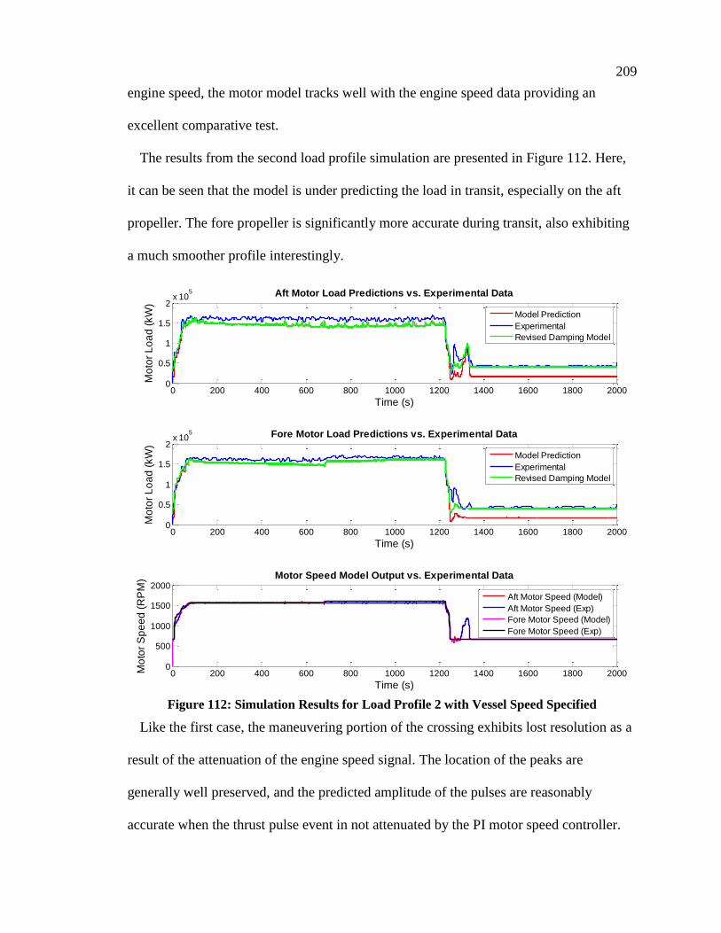
209

engine speed, the motor model tracks well with the engine speed data providing an

excellent comparative test.

The results from the second load profile simulation are presented in Figure 112. Here,

it can be seen that the model is under predicting the load in transit, especially on the aft

propeller. The fore propeller is significantly more accurate during transit, also exhibiting

a much smoother profile interestingly.


Like the first case, the maneuvering portion of the crossing exhibits lost resolution as a

result of the attenuation of the engine speed signal. The location of the peaks are

generally well preserved, and the predicted amplitude of the pulses are reasonably

accurate when the thrust pulse event in not attenuated by the PI motor speed controller.

0 200 400 600 800 1000 1200 1400 1600 1800 20000

0.5

1

1.5

2x 10

5

Time (s)

Mo

tor

Lo

ad

(kW

)


Model Prediction

Experimental


0 200 400 600 800 1000 1200 1400 1600 1800 20000

0.5

1

1.5

2x 10

5

Time (s)

Mo

tor

Lo

ad

(kW

)


Model Prediction

Experimental


0 200 400 600 800 1000 1200 1400 1600 1800 20000

500

1000

1500

2000

Time (s)

Mo

tor

Sp

ee

d (

RP






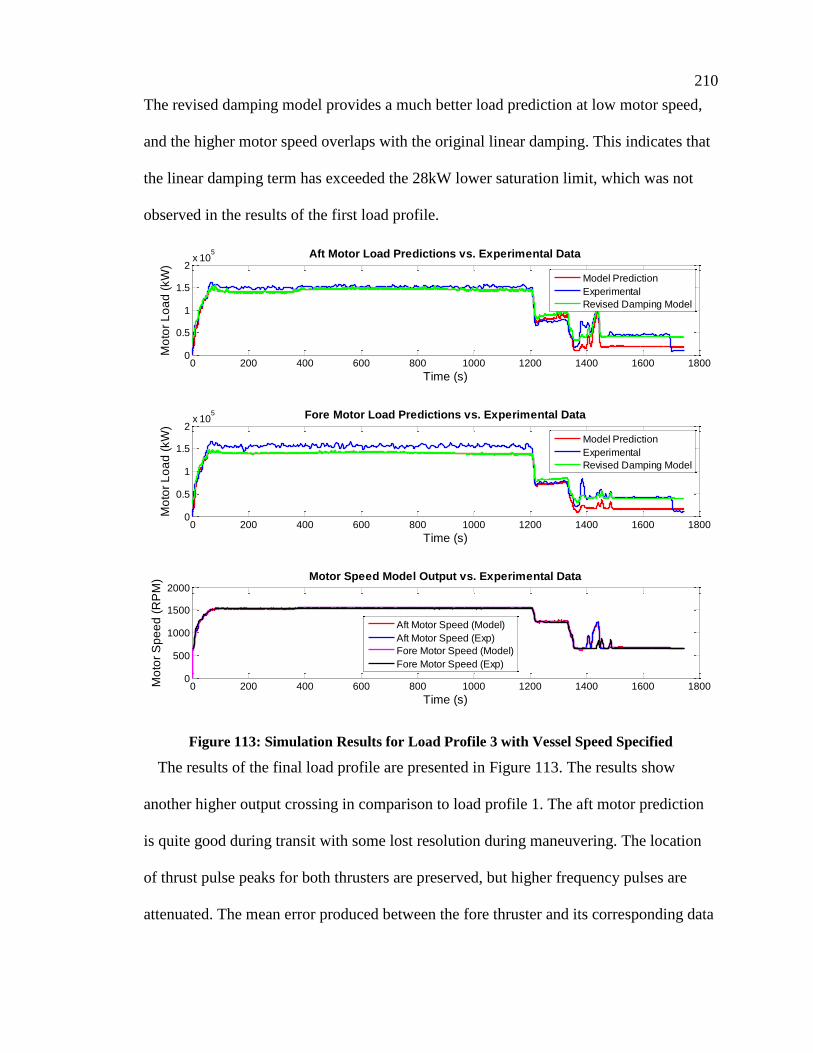
210

The revised damping model provides a much better load prediction at low motor speed,

and the higher motor speed overlaps with the original linear damping. This indicates that

the linear damping term has exceeded the 28kW lower saturation limit, which was not

observed in the results of the first load profile.


The results of the final load profile are presented in Figure 113. The results show

another higher output crossing in comparison to load profile 1. The aft motor prediction

is quite good during transit with some lost resolution during maneuvering. The location

of thrust pulse peaks for both thrusters are preserved, but higher frequency pulses are

attenuated. The mean error produced between the fore thruster and its corresponding data

0 200 400 600 800 1000 1200 1400 1600 18000

0.5

1

1.5

2x 10

5

Time (s)

Mo

tor

Lo

ad

(kW

)


Model Prediction

Experimental


0 200 400 600 800 1000 1200 1400 1600 18000

0.5

1

1.5

2x 10

5

Time (s)

Mo

tor

Lo

ad

(kW

)


Model Prediction

Experimental


0 200 400 600 800 1000 1200 1400 1600 18000

500

1000

1500

2000

Time (s)

Mo

tor

Sp

ee

d (

RP






211

is the largest of any of the simulation. Interestingly, the experimental data collected for

one engine seems to consistently produce larger error regardless of whether it lies in the

fore or aft position. The data collected from the other engine consistently produces better

results regardless of vessel direction.

By investigating the load profile, it can clearly be observed that a significant amount of

energy is needlessly dissipated while the ferry is in berth with the existing diesel

architecture. Diesel engines have a prescribed idle speed and the thruster system must

maintain a minimum shaft load to keep the clutches engaged. The integrated

gearbox/hydraulic systems are the dominant sources of energy dissipation while the

engines idle in berth. Furthermore, an unnecessarily high level of propeller load is

generated as a consequence of the idle speed constraint. By converting to an electric

propulsion system, the propeller can be reduced to zero speed to achieve energy savings,

provided that the ship is adequately restrained by the marine structures. The energy

savings from zero speed operation in berth, including the contribution from a linear

damping approximation for gearbox losses are tabulated in Table 31. Note that load

profile 3 is significantly smaller, as this was the end-of-day crossing with only the offload

cycle represented.

Table 31: Potential Energy Savings from Zero-Speed Propeller Operation In-Berth

Load

Profile

In-Berth

Duration

(s)

Estimated

Energy Savings

(kWh)

1 894 8.44

2 647 5.99

3 246 2.44

A more detailed decomposition of the gearbox and hydraulic system load/loss

characteristics would provide a more accurate estimate for additional savings. As an

aside, a mechanically-driven PTO hydraulic system powered by engine’s output shaft is

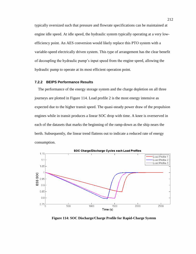
212

typically oversized such that pressure and flowrate specifications can be maintained at

engine idle speed. At idle speed, the hydraulic system typically operating at a very low-

efficiency point. An AES conversion would likely replace this PTO system with a

variable-speed electrically driven system. This type of arrangement has the clear benefit

of decoupling the hydraulic pump’s input speed from the engine speed, allowing the

hydraulic pump to operate at its most efficient operation point.

7.2.2 BEIPS Performance Results

The performance of the energy storage system and the charge depletion on all three

journeys are plotted in Figure 114. Load profile 2 is the most energy intensive as

expected due to the higher transit speed. The quasi-steady power draw of the propulsion

engines while in transit produces a linear SOC drop with time. A knee is overserved in

each of the datasets that marks the beginning of the ramp-down as the ship nears the

berth. Subsequently, the linear trend flattens out to indicate a reduced rate of energy

consumption.

Figure 114: SOC Discharge/Charge Profile for Rapid-Charge System

213

Once the ship is in berth, the charging system is engaged with a 5C continuous current

fast-charge and the SOC increases approximately linearly at first until the maximum

voltage is achieved. The charge then exponentially tapers to zero, but at a rate that seems

unfeasibly high. The battery parameters were verified in the model, and no error could be

identified; however, the equivalent circuit parameter data from Cleary et al. [43] did not

provide good resolution for circuit parameters at high SOC which could help explain the

results. Regardless, the CC and CV algorithms function as intended and the results show

a 20% DoD in the most energy intensive cycle.

Lastly, the modeling results allow for investigation of component efficiencies

throughout the cycle. The individual component efficiencies for each load profile are

plotted versus time in Figure 115. During transit the motors, battery system, and

converters are all operating in excess of 92% across all three cycles. The motor

efficiencies drop below 90% as the ship begins its ramp-down, but maintain >80%

efficiency throughout the entire cycle with exception to short-term transient events.

During loading/offloading, the motors maintain an efficiency above 83% using the

same operational profiles as the diesel engines, though the motors could be reduced to

zero speed for energy savings.

The relatively small current draw from the battery while in transit produces little ohmic

loss dissipation in the battery model, leading to a high efficiency. Once a rapid charge

cycle is engaged, a sharp decline in efficiency is observed as more energy is being

dissipated within the battery’s internals and electrochemical reactions. Despite the

increased ohmic losses during charging, the efficiency remains above 90%.

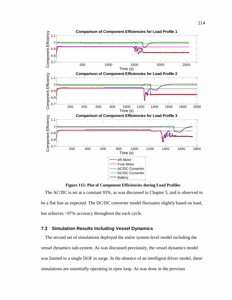
214

Figure 115: Plot of Component Efficiencies during Load Profiles

The AC/DC is set at a constant 93%, as was discussed in Chapter 5, and is observed to

be a flat line as expected. The DC/DC converter model fluctuates slightly based on load,

but achieves >97% accuracy throughout the each cycle.

7.3 Simulation Results Including Vessel Dynamics

The second set of simulations deployed the entire system-level model including the

vessel dynamics sub-system. As was discussed previously, the vessel dynamics model

was limited to a single DOF in surge. In the absence of an intelligent driver model, these

simulations are essentially operating in open loop. As was done in the previous

500 1000 1500 2000 25000.7

0.8

0.9

1

1.1

Time (s)

Com

ponent E

ffic

iency Comparison of Component Efficiencies for Load Profile 1

200 400 600 800 1000 1200 1400 1600 1800 20000.7

0.8

0.9

1

1.1

Time (s)

Com

ponent E

ffic


200 400 600 800 1000 1200 1400 1600 18000.7

0.8

0.9

1

1.1

Time (s)

Com

ponent E

ffic


200 400 600 800 1000 1200

0.75

0.8

0.85

0.9

Time (s)

Com

ponent E

ffic


200 400 600 800 1000 1200 1400 1600 1800 20000.7

0.8

0.9

1

1.1

Time (s)

Com

ponent E

ffic


Aft Motor

Fore Motor

AC/DC Converter

DC/DC Converter

Battery

200 400 600 800 1000 1200 1400 1600 18000.7

0.8

0.9

1

1.1

Time (s)

Com

ponent E

ffic


Aft Motor

Fore Motor

AC/DC Converter

DC/DC Converter

Battery

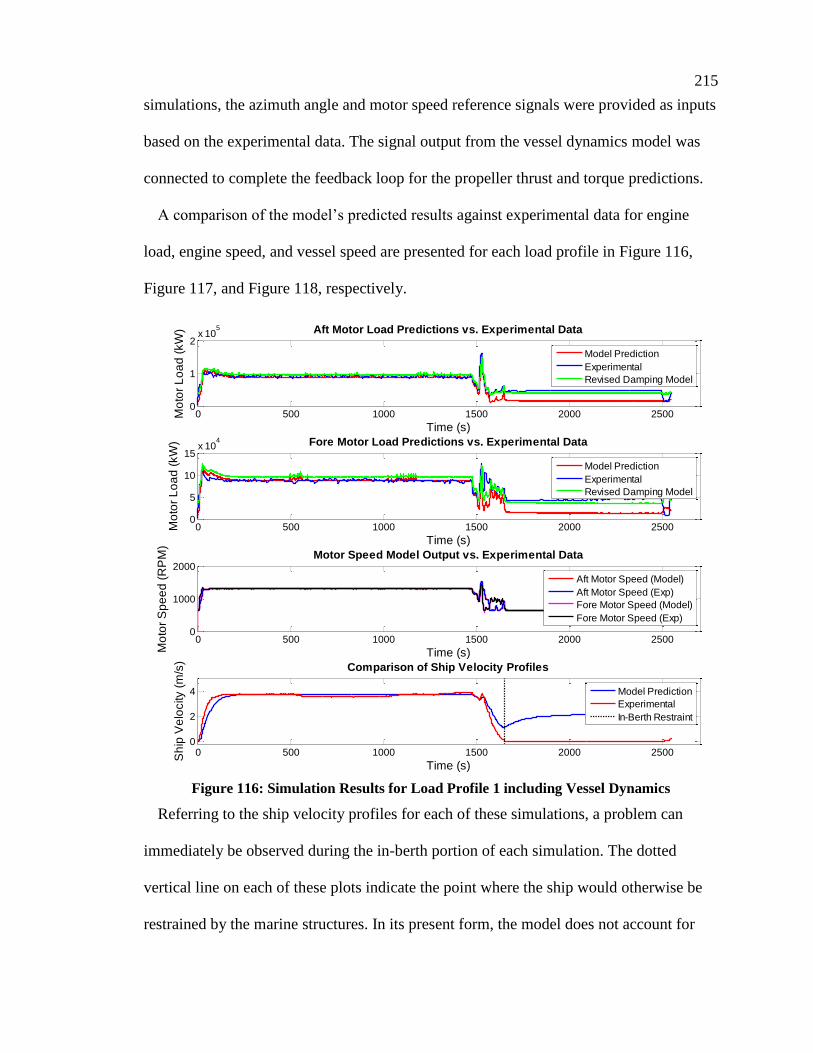
215

simulations, the azimuth angle and motor speed reference signals were provided as inputs

based on the experimental data. The signal output from the vessel dynamics model was

connected to complete the feedback loop for the propeller thrust and torque predictions.

A comparison of the model’s predicted results against experimental data for engine

load, engine speed, and vessel speed are presented for each load profile in Figure 116,

Figure 117, and Figure 118, respectively.

Figure 116: Simulation Results for Load Profile 1 including Vessel Dynamics

Referring to the ship velocity profiles for each of these simulations, a problem can

immediately be observed during the in-berth portion of each simulation. The dotted

vertical line on each of these plots indicate the point where the ship would otherwise be

restrained by the marine structures. In its present form, the model does not account for

0 500 1000 1500 2000 25000

1

2x 10

5

Time (s)

Mo

tor

Lo

ad

(kW

) Aft Motor Load Predictions vs. Experimental Data

Model Prediction

Experimental


0 500 1000 1500 2000 25000

5

10

15x 10

4

Time (s)

Mo

tor

Lo

ad

(kW

) Fore Motor Load Predictions vs. Experimental Data

Model Prediction

Experimental


0 500 1000 1500 2000 25000

1000

2000

Time (s)Mo

tor

Sp

ee

d (

RP

M)

Motor Speed Model Output vs. Experimental Data





0 500 1000 1500 2000 25000

2

4

Time (s)

Sh

ip V

elo

city (

m/s

)

Comparison of Ship Velocity Profiles

Model Prediction

Experimental

In-Berth Restraint

216

this restraining force, and the ship appears to accelerate while in berth; consequently, the

results beyond the dotted line are neglected.

Beginning with load profile 1, the predicted powertrain loads with 1-DOF motion are

very similar to those observed in the previous sections. The velocity profile predicted by

the model shows a slower acceleration during ramp-up which leads to an increased load

on the propulsion motors during the acceleration. The increased load is intuitive because

propeller thrust and torque production increases as advance ratio decreases in the first

quadrant.

The reduced acceleration and deceleration rates naturally point to an inertial

discrepancy, especially since the velocity in transit is relatively accurate. There is

uncertainty in the inertial properties because the variation in vessel loading could not

been easily accounted for in the analysis. If we recall from Chapter 4, the inertial

properties were taken from a set operating condition outlined in the ship’s stability book.

The dynamic braking that occurs as the ship approaches the berth is not well represented,

partially because the model inertia will likely be higher than was present during the

experiment. The normal departure condition identified in the stability book can

conclusively be determined as an over-estimate, because the loading condition specified

is not typically encountered in normal operation.

The dynamic braking performed by the driver on the real ship is executed to achieve a

near-zero forward speed to gently make contact with the marine structures. Here, the

model predicts an approximate 1 m/s forward speed as the ship enters berth. After

experimenting with the simulations with reduced inertia, it was concluded that not all of

this discrepancy can be attributed to the inertial parameters. Other problematic areas

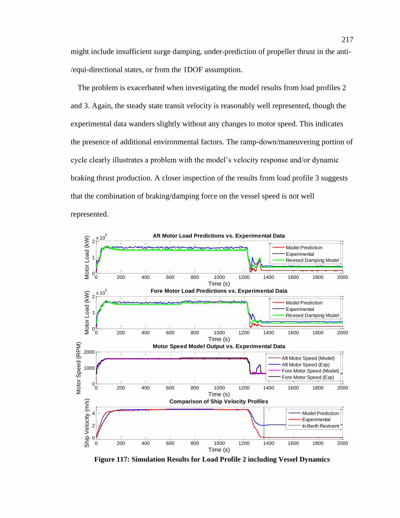
217

might include insufficient surge damping, under-prediction of propeller thrust in the anti-

/equi-directional states, or from the 1DOF assumption.

The problem is exacerbated when investigating the model results from load profiles 2

and 3. Again, the steady state transit velocity is reasonably well represented, though the

experimental data wanders slightly without any changes to motor speed. This indicates

the presence of additional environmental factors. The ramp-down/maneuvering portion of

cycle clearly illustrates a problem with the model’s velocity response and/or dynamic

braking thrust production. A closer inspection of the results from load profile 3 suggests

that the combination of braking/damping force on the vessel speed is not well

represented.


0 200 400 600 800 1000 1200 1400 1600 1800 20000

1

2x 10

5

Time (s)

Mo

tor

Lo

ad

(kW


Model Prediction

Experimental


0 200 400 600 800 1000 1200 1400 1600 1800 20000

1

2x 10

5

Time (s)

Mo

tor

Lo

ad

(kW


Model Prediction

Experimental


0 200 400 600 800 1000 1200 1400 1600 1800 20000

1000

2000

Time (s)Mo

tor

Sp

ee

d (

RP

M)






0 200 400 600 800 1000 1200 1400 1600 1800 20000

2

4

Time (s)

Sh

ip V

elo

city (

m/s

)


Model Prediction

Experimental

In-Berth Restraint

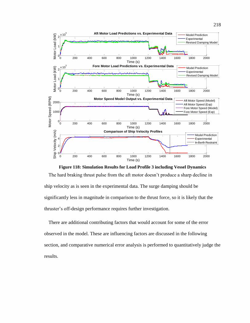
218


The hard braking thrust pulse from the aft motor doesn’t produce a sharp decline in

ship velocity as is seen in the experimental data. The surge damping should be

significantly less in magnitude in comparison to the thrust force, so it is likely that the

thruster’s off-design performance requires further investigation.

There are additional contributing factors that would account for some of the error

observed in the model. These are influencing factors are discussed in the following

section, and comparative numerical error analysis is performed to quantitatively judge the

results.

0 200 400 600 800 1000 1200 1400 1600 1800 20000

1

2x 10

5

Time (s)

Mo

tor

Lo

ad

(kW


Model Prediction

Experimental


0 200 400 600 800 1000 1200 1400 1600 1800 20000

1

2x 10

5

Time (s)

Mo

tor

Lo

ad

(kW


Model Prediction

Experimental


0 200 400 600 800 1000 1200 1400 1600 1800 20000

1000

2000

Time (s)Mo

tor

Sp

ee

d (

RP

M)






0 200 400 600 800 1000 1200 1400 1600 1800 20000

2

4

Time (s)

Sh

ip V

elo

city (

m/s

)


Model Prediction

Experimental

In-Berth Restraint

219

7.4 Analysis and Discussion of Results

7.4.1 Model vs. Experimental Direct Comparison

The results from all six simulation studies show relatively good correlation with the

experimental data collected, especially during steady in-transit operation. The original

linear damping assumption for the mechanical power transmission system did not capture

the PTO effects of the hydraulic system, leading to poor results while the ship was at low

output. The revised damping model, which maintained a minimum mechanical base load,

provided a more accurate representation during low power output conditions but has no

physical basis. The revised damping model combined with the propeller torque is still

under-predicting engine load at higher output; therefore, the PTO damping model really

needs to be examined in further technical detail to pinpoint the source of error. The wake

fraction sub-system will also influence propeller load, so it could also be a contributing

factor.

The dynamics of the PTO system are likely a contributor to the increased error seen in

the maneuvering portion of the cycle. High frequency fluctuations are observed in the

experimental engine speed data which also correlates to observable load peaks that are

not likely produced by the propeller. These observations naturally point to variations in

the PTO hydraulic system during dynamic conditions. The hydraulic system provides the

actuation force for rotating the azimuthing thrusters during maneuvers. The PTO model

should be linked to azimuthing thruster model to give a more physical interpretation of

the dynamic load, but little information was available from the manufacturer to develop a

suitable mathematical relationship.

A summary of the mean and maximum instantaneous relative error observed for each

cycle, decomposed by load profile and operating regime, is presented in Table 32. The

220

experimental values were assumed to be correct, and the relative error was computed

using the equation,

𝑎𝑏𝑠(𝑃𝑒𝑥𝑝 − 𝑃𝑚𝑜𝑑𝑒𝑙)

𝑃𝑒𝑥𝑝 ( 7-1 )

Initial start-up conditions for the model and erroneous data points have been omitted in

the error analysis. With both simulation configurations, the in-transit is well represented

by the model generally yielding results less than 10% mean relative error between

predicted load and actual load. As discussed previously, the maneuvering portion is

definitely more problematic. The mean relative error diverges with the generally around

20% even with the revised damping model. At constant output in berth, revised damping

model produces good results with mean relative error less than 7%.

Table 32: Instantaneous Relative Error Analysis of Simulation Results

It should be noted that the data collected for Engine 1 consistently provided the highest

discrepancy across each simulation. Recalling that load profiles 1 and 3 have this engine

in the fore position, and load profile 2 has this in aft position, this pattern can be observed

regardless of position. Engine 2 provided much better results by comparison. It is

possible that the ECM computations of engine load contain some error due to improper or

Mean Max Mean Max Mean Max Mean Max Mean Max Mean Max

LP1 (No Vessel Dynamics) 3.8% 16.0% 33.7% 62.5% 61.8% 64.8% 3.0% 16.1% 35.7% 79.7% 60.1% 62.6%

LP1 (Vessel Dynamics) 4.1% 21.0% 35.8% 69.0% - - 3.5% 16.9% 33.8% 79.7% - -





Mean Max Mean Max Mean Max Mean Max Mean Max Mean Max







In-Berth

Instantaneous Relative Error Analysis

For Motor Model Data (Linear Damping)

In-Transit Ramp-Down/Man. In-Berth

For Motor Model Data Revised Damping)

Aft Motor Model Data (Linear Damping)

In-Transit Ramp-Down/Man. In-Berth

Aft Model Data Revised Damping)

In-Transit Ramp-Down/Man. In-Transit Ramp-Down/Man.In-Berth

Load Profile

Load Profile

221

unrepresentative calibration. The engines had just been serviced and dynamometer tested

before the data acquisition system was installed, so it’s unlikely this error can fully be

placed on improper calibration. Future validation will require direct measurement the

output shaft to the engine using strain gaging and rotational speed sensors.

The objective of this work was to establish an integrated propulsion modeling tool that

was suitable for architectural design studies to assess overall system performance. The

simulation framework generally achieves <20% mean error, which can likely be

improved upon with minor adjustments to the model. The model has been parameterized,

for the most part, using only numerical analysis techniques and manufacturer datasheets.

This implies that the approach can be applied during the design stage when operational

data is not available.

In general, the correlation between the experimental data and model predictions was

fairly good, especially when the velocity profile constrained to known operational profile;

however, prediction of load pulses and dynamic actuation forces during maneuvers

approach berth were a bit problematic due to attenuation by the electric drive’s PI

controller.

7.4.2 Model and Sub-System Uncertainties

The model implementation and parameterization has been performed using a

combination of computational analysis, empirical coefficients, experimental data, and

educated assumptions. Section 6.4 described the sources of uncertainty in the

experimental data, some of which will have propagated into the modeling results. Due to

the experimental limitations imposed by testing a ship while in-service, there are few

opportunities to run prescribed and targeted tests that could quantify uncertainties and

222

errors in the individual subsystems. A more extensive set of parameterization data for the

ship hull could also be developed using additional CFD experiments. Though CFD is a

powerful design tool, the time required to generate the full spectrum of data is almost

unfeasible, even with a super computing cluster like Westgrid.

In order to highlight the relative degrees of accuracy/uncertainty in the sub-

components, Table 33 provides a qualitative ranking of each sub-system to the most

significant areas that will improve the model’s performance. The relative degree of

confidence has been assessed based on the results presented in section 7.3, and the

parameterization process/assumptions that went into the model’s construction. The

PTO/damping model, vessel dynamics model, and thrust deduction factor sub-models

carry the most uncertainty. The following sections will provide specific details on the

problematic areas within the model and how they can be addressed in future work.

Table 33: Relative Modeling Uncertainty and Degree of Confidence

Sub-Model Relative Level of

Confidence Description

Thrust/Torque Coefficients

High/Medium High confidence in 1st quadrant, medium confidence in

angular/opposing flow conditions

Thrust Deduction Factor

Low Incomplete dataset t(u)

Large scatter in experimental data used to compute t

Wake Fraction High/Medium Based on high resolution CFD results, though results

differ from original model test data

Battery System High Validated using published experimental data

Electric Drive Systems

High Validated using component data

PTO Model Medium/Low

Estimated from experimental data, no dynamics associated

Does not consider physical loading factors during actuation of the thruster tower

GB Torque Damping Model

Medium Estimated using manufacturer information

Vessel Dynamics Model

Medium Surge CFD results under-predicts versus original ship

design data

Over-estimate of mass and inertial parameters

223

Hydrodynamic coefficient errors in some of 6DOF matrix entries

Excellent results for in-transit on approximate constant course with unified seakeeping/maneuvering model

Errors developing during maneuvering and large course and speed deviation with vessel dynamics equation

7.4.2.1 Rotational Damping Characteristics and PTO

The rotational damping characteristics of the gearbox system were simplified to a

linearly proportional model relative to rotational speed. Coulomb damping and other

frictional components are often introduced into the equation as well, for example see

Pivano [79], provided that experimental data can be secured. Detailed experimentation

was not possible with the full-scale thruster, and such an experiment would require a

relatively involved instrumentation setup making it somewhat unfeasible. This remains

one of the major areas from improvement. The best course of action for firming up this

model would be to engage the manufacturer for any testing results that they may have.

Further to the gearbox, the dynamics and loss characteristics of the hydraulic PTO

system was unaccounted for in the original simulation model. With the revised damping

model, the 28-30kW discrepancy between model results and experimental data was

attributed to the hydraulic system, but this requires further investigation to be conclusive.

The performance characteristics of the hydraulic pump at various input shaft speeds,

pressures, and flow rates would allow for a preliminary physics-based model to be

constructed. The loading characteristics would then need to be mapped to the azimuthing

thruster actuation system to relate the physical load back to the IPS.

7.4.2.2 Inertial Discrepancies

The inertial properties of the ship were assumed constant across all load profiles. This

assumption was based on a prescribed operating condition in the stability book. The exact

224

vessel loading data, including passenger/vehicle count, could be retrieved with BC

Ferries’ historic logs to improve the inertial parameterization. This effort would likely

assist in quantifying the upper bound for error in the inertial properties, but will still carry

some uncertainty because logs only capture the number of vehicles and not mass

explicitly. The assumed mass and inertial specifications can be conclusively deemed as

over-estimates simply because the loading condition portrayed in the stability book is

rarely achieved during operation.

7.4.2.3 Low Speed Surge Damping Model

It has been commonly documented in related work that the linear/non-linear matrix

decomposition can under-predict surge damping characteristics at lower vessel speed, see

for example Fossen [63]. Dynamic positioning control systems often use different

damping models for low-speed, and in-transit operation. This would be consistent with

the result seen in this study. Under-prediction of damping would account for the slower

deceleration seen during ramp-down. A transient CFD analysis replicating the ramp-

down, or a vessel coasting experiment might provide more insight into the true damping

characteristics of the ship.

7.4.2.4 Thrust Deduction Factor

The thrust deduction factor is definitely the sub-system that carries the most

uncertainty. The original intent was to conduct a series of self-propelled CFD studies to

quantify this additional hull resistance term as a function of forward speed. Unfortunately

the configuration of these analyses proved to be somewhat problematic and the results

could not be generated within the time period needed. As a result, this term was

computed using experimental data and the bare hull CFD results. This produced an

225

incomplete set of data points which exhibited a large degree of scatter. The results were

averaged and fit to a parabolic model which may or may not be appropriate.

This subsystem could account for some of the issues observed in the vessel dynamics

model. A more comprehensive treatment of the thrust deduction factor is required to

improve the results, and should be one the immediate areas of focus in future work. This

can be done either through additional CFD studies or from scale model tow tank testing.

7.4.2.5 1-DOF Surge System Assumption

The 1-DOF assumption used in this work would have accounted for some of the

discrepancies seen in the model, especially during the ramp-down/maneuvering portion

of the cycle. The GPS data collected is purely a measurement of velocity magnitude and

does not factor vector components of the body’s motion. Referring back to Figure 101, it

can be seen that the ship actually drifts laterally as it comes into berth for both terminals.

During this maneuver, the sway component of velocity will be significant. With the 1-

DOF assumption, the GPS velocity magnitude was assumed to be entirely in surge. In

actual fact, the velocity is split between surge and sway. Inclusion of the additional DOF

would likely reconcile some of the dynamic braking issues observed.

In order to investigate the hull model’s performance more thoroughly, an intelligent

driver/auto-pilot model will need to be developed along with a course tracking algorithm.

The trajectories collected in the data acquisition study can be used to produce the desired

path. This will allow for a more direct comparison of the vessel dynamics model with the

dynamics of the real ship in a closed loop form. This is not a trivial task, mainly because

of the Klitsa’s thruster configuration. The manipulation of azimuthing thrusters is an

optimal control problem, because there are an infinite number of solutions for achieving

226

the same result. The development of a driver model will require a significant

development effort, but provides an excellent academic project moving forward.

7.4.2.6 Signal Attenuation and Lost Resolution in Data

The data collected as part of DAQ experiment contained a fair amount of noise which

was digitally filtered using post-processing. The resulting output signal exhibited some

lost resolution, though the mean value tracked well with the raw data. The higher

frequency engine speed fluctuations observed in the experimental data during

maneuvering contained some high frequency fluctuations that were attenuated by the

motor drive’s PI controller. The combined signal error and attenuation of higher

frequency dynamics drastically under-predicted some of thrust peaks observed in the load

cycles. The combined effect of these two factors accounts for a portion of the model’s

error, though this is likely to be negligible in comparison to the error contained in the

PTO/damping model.

227

Chapter 8 Conclusions and Recommendations

8.1 General Summary and Conclusions

This thesis has systematically developed a methodology for creating parametric time-

domain ship models for the study of hybrid and electric propulsion systems. As an

illustrative example, this work modeled a BEIPS architecture as a case study to predict

the performance of this architecture with the hull and thruster system of BC Ferries’ M.V.

Klitsa. The power system was modeled using a blended modeling approach that utilized

both power loss and AVM models to balance accuracy with computational efficiency.

The methodology and model development process outlined in this work relied heavily

on the use of computational fluid dynamics for parameterization. CFD was deployed for

analysis of the bare hull resistance at a prescribed set of forward speeds that spanned the

operating range of the vessel. Furthermore, a design of experiment was devised to

generate the necessary data to parameterize a lookup surface of thrust and torque

coefficients to quantifying thruster performance under all potential operating conditions.

The BEIPS component models were based off commercially available components,

with parameterization primarily from equipment datasheets and manufacturer

information. The energy storage system was modeled off experimental data published by

Cleary et al. [43]. The components were individually validated against manufacturer or

published data to ensure proper implementation.

Performance comparison and validation of the ship model was achieved using

experimental data collected from the Klitsa while in operation. A data acquisition system

was installed onboard the ship to record the energy demands and typical load/velocity

operating profiles. Using this data, three representative load profiles were created to

simulate low, medium, and high output crossings. The engine speed and propeller

228

azimuth angle signals collected as part of the experiment, served as an open loop driver

inputs for the model to recreate the real vessel crossing and actuation.

The performance comparison and model validation was done in two parts. The first set

of simulations disabled the vessel dynamics model, and applied the experimental time

series data for the ship velocity profile as a time-synchronized input. This allowed for a

direct comparison of the model’s performance in predicting propulsive loads, along with

the other influencing subsystems.

In comparison to the experimental operational data, the simulation results were

satisfactory but definitely requires some improvement to increase the fidelity. The PTO

and linear damping characteristics of the mechanical power transmission system

definitely require additional investigation to better define the dynamic loading

characteristics, especially during transient conditions while maneuvering. It was found

that when the ship’s velocity profile was well represented, the propulsive loads were

sufficiently accurate for high-level architectural design studies.

Upon incorporating the vessel dynamics into the simulation, each simulation exhibited

a reduced acceleration and deceleration rate in comparison to the actual ship. This

discrepancy immediately points to an over-estimate of the ship’s inertial properties,

though the surge damping characteristics, thrust deduction factor, and the 1-DOF motion

may have also been contributing factors to the discrepancy.

The primary objective of this entire effort was to develop a simulation platform that

can assess the performance of different propulsion system architectures in the context of

energy consumption, and system efficiency. This study illustrated the effectiveness of

this modeling and simulation process by investigating the power system conversion

229

efficiency associated with a battery-electric propulsion system. The energy consumption

estimates and their relative error in comparison to experimental data are provided in

Table 34. The experimentally determined consumption has been taken to be the correct

value, and the relative error in energy consumption is expressed as,

𝑎𝑏𝑠(𝐸𝑒𝑥𝑝 − 𝐸𝑚𝑜𝑑𝑒𝑙)

𝐸𝑒𝑥𝑝 ( 8-1 )

Using the revised damping model, the estimated energy consumption is within good

agreement with the experimentally calculated values. This despite several simplifying

assumptions, thereby proving the effectiveness of this approach for high level

architectural analysis.

Table 34: Energy Consumption Results and Relative Error Against Experimental

Load Profile

Total Propulsive Motor Energy Consumption (kWh)

Experimental Data Model Data (Linear

Rotational Damping) Model (Revised Damping)

In Transit Man.

In Berth

In Transit Man.

In Berth

In Transit Man.

In Berth

LP1 (No Vessel Dyn.) 72.5 7.1 20.6 71.8 4.8 8.3 78.1 6.6 19.4

LP1 (Vessel Dyn.) 72.5 7.1 20.6 72.0 4.8 - 78.3 6.7 -

LP2 (No Vessel Dyn.) 108.4 4.6 15.6 100.5 2.6 6.2 100.8 3.9 14.5

LP2 (Vessel Dyn.) 108.4 4.6 15.6 101.1 2.6 - 101.5 3.9 -

LP3 (No Vessel Dyn.) 100.8 10.1 5.1 93.5 8.1 2.4 93.9 10.6 5.5

LP3 (Vessel Dyn.) 100.8 10.1 5.1 92.2 8.0 - 92.5 10.5 -

Load Profile

Relative Error - Energy Consumption Model Data (Linear

Rotational Damping) Model (Revised Damping)

In Transit Man.

In Berth

In Transit Man.

In Berth

LP1 (No Vessel Dyn.) 0.9% 32.4% 59.7% 7.7% 6.5% 5.7%

LP1 (Vessel Dyn.) 0.6% 31.7% - 8.0% 5.9% -

LP2 (No Vessel Dyn.) 7.3% 43.3% 60.5% 7.0% 16.1% 7.2%

LP2 (Vessel Dyn.) 6.7% 43.0% - 6.4% 15.8% -

LP3 (No Vessel Dyn.) 7.3% 19.5% 53.1% 6.9% 5.6% 7.8%

LP3 (Vessel Dyn.) 8.6% 21.2% - 8.2% 4.0% -

230

The model results from the BEIPS simulation were plausible and provided an excellent

illustration how this platform can be deployed. The battery system model, which was

based on pack-level experimental data, performed very well; however, its performance

above 90% SOC has some uncertainty because of the limited dataset provided by Cleary

et al. [43]. Combined with the rapid-charge model, the results demonstrate that a battery-

electric ship is technologically feasible for this application, though cost factors have not

been considered in the analysis. With the ESS design assumptions, the longevity of the

battery pack, with the deepest DoD of 20%, would likely exceed 30,000 cycles. This

corresponds to approximately 5 years of operation at 18 crossing per day. More advanced

degradation models can be incorporated in the future.

8.2 Summary of Recommendations

The modeling and validation approach presented in this work was an ambitious effort

to assess the applicability of using model based design for advanced marine propulsion

systems, in a manner that is similar to the development process used in the automotive

industry. Though the initial results produced in this work have shown that this approach

can be effective even with simplifying assumptions, there are numerous sources of error

that need to be further investigation to determine what level of fidelity can actually be

achieved with this framework.

The major limitation of this work is that the experimental results used for validation

carry a significant amount of uncertainty due to the uncontrolled environment. Section

6.4 presented a detailed discussion of the experimental uncertainties, and highlighted the

difficulty in quantifying the error found in the data. Without conducting an extensive set

of experiments and sea trials with the ship, it is difficult to categorically validate the

231

simulation framework. The level of experimentation required to produce high quality

validation data is unfeasible when the ship is in service, and is very difficult to arrange.

With that said, the data collected does provide some insight into problematic areas

within the model. This section summarizes major areas for improvement and future study

that will help reconcile the discrepancies observed in the simulation results. Given the

tightly coupled interaction between sub-components, the process of increasing the

model’s fidelity might benefit from a sensitivity analysis. Further experimentation with

the vessel is definitely recommended, as this would provide the most effective

mechanism to identify the dominant sources of error. The following sub-sections present

the immediate recommendations for increasing the model fidelity.

8.2.1 Additional Experimentation

Performing an additional set of more detailed experiments would provide the best

means for confirming the model’s parameterization and assumptions. The experimental

setup developed in this work could mostly be reused; however, the ECM’s computation

of load should be replaced by a direct power measurement from strain gages and a

rotational speed sensor. Similarly, the input shaft to the hydraulic pump should also be

equipped to with a direct mechanical power measurement system to quantify the PTO’s

dynamic load characteristics. Ideally, a run-up/coast-down experiment would be

conducted on the azimuthing propeller gearbox in dry-dock would help study the

damping characteristics of the gearbox in detail, but this test is likely unfeasible.

A series of sea trials tests at a prescribed displacement would help parameterize the

vessel dynamics model and the inertia model. A straight-line coast down experiment in

calm seas would provide a meaningful set of data for investigating the surge damping

232

model. Similarly, pure-sway and pure-yaw experiments would provide a dataset for

validating the maneuvering coefficients/model.

8.2.2 PTO and Rotational Damping model

A more accurate representation of the PTO hydraulic system is the first logical step in

attempting to reconcile the load discrepancies seen in the simulation results. The PTO’s

loading characteristics and representative dynamics need to correlate to the physical

system that it is driving, in this case it is the actuation of the azimuthing thrusters.

Information on this system was requested of the manufacturer, but the pump

characteristics and azimuth tower loading details could not be obtained. The power

required to rotate the azimuthing tower at forward speed could be approximated using

simple drag assumptions based on projected area of the tower/propeller as a function of

azimuth angle. Equivalently, CFD could be utilized to provide more accurate results.

The rotational damping model developed in this work lumped the gearbox damping

characteristics and the PTO into a single model. These effects need to be separated and

studied individually. The lumped model assumed a constant 28kW loss as a minimum for

the combined load, and a linear speed-dependent damping function was assumed when

the linear loss relationship exceeded 28kW. This lumped model produced an under-

estimate of damping at higher output, and an over-estimate at lower output indicating the

real relationship is not well suited to the linear assumption.

The best course of action for quantifying gearbox losses and establishing an

appropriate mathematical relationship is to first develop a good representation for the

PTO system. Once this is established, the PTO and propeller loads can be subtracted from

the experimental data collected to produce an estimate for the gearbox damping loads.

233

This residual dataset can then be used to investigate the mathematical relationship for

gearbox damping. A survey of literature can perhaps provide additional insight into the

expected behaviour and losses of right-angle drive gearboxes.

8.2.3 Refinement of Inertial Properties

The mass properties assumed for the ship can be conclusively deemed as over-

estimates. A preliminary mass sensitivity study was performed to determine the impact of

increased mass on the acceleration/deceleration rates from the model. This initial

investigation showed that a more realistic estimate of mass did have a positive impact on

reducing the simulation error, it will definitely not account for the entire discrepancy.

The interplay between the thrust deduction factor, wake fraction, propeller model,

surge damping, and ship mass will simultaneously influence the simulation results.

Wherever possible, these sub-components needs to be isolated and refined as best as

possible to pinpoint the major source of error. Revising the mass properties is relatively

low hanging fruit in that it’s a simple parameter change that can be better estimated using

historical passenger/vehicle logs from BC Ferries, provided that they can be obtained.

8.2.4 Vector Decomposition of GPS Speed Data

The raw GPS speed data was assumed to be entirely directed in the surge direction.

This assumption is valid for in-transit operation, but may have introduced significant

error when the ship is maneuvering into berth. The output from the heading sensor and

GPS waypoints provide a method to decompose the reported ship velocity into surge,

sway, and yaw components. This was not done initially because of problems with the

signal output from the Maretron gyrocompass. The raw data is still available, and the

issue can be resolved by accessing the Maretron configuration software then exporting

234

the data to a convenient format. This will process will also be very useful in the

development of the auto-pilot model for full 6-DOF simulation.

8.2.5 Thrust Deduction Factor Parameterization

The thrust deduction factor model was a rather crude assumption based on

experimental data and a simple parabolic mathematical relationship to account for its

speed dependency. The parabolic assumption could be a major contributing factor to the

slower acceleration and deceleration with the vessel dynamics model. Self-propelled

CFD analysis would provide a means of resolving the actual thrust deduction factor as a

function of forward speed. The initial efforts attempted were too ambition as they sought

to resolve the rotating propeller along with motion of the ship using overset meshing. The

number of cells produced by this approach was computationally unfeasible, and the

analyses were abandoned. Instead, the self-propelled model should use an actuator disk to

represent the propeller in order to simplify the analysis.

8.3 Concluding Remarks

The methodology for ship model development outlined in this work, and its illustration

through a case study of the M.V. Klitsa, has proven to be an effective strategy for

predicting high-level performance of the vessel in the design stage. The model developed

definitely requires more development and refinement to improve accuracy before it could

be used for detailed energy management control system development, or rigorous power

system analysis. The ship model developed for the Klitsa can serve as an excellent

starting point for future studies, and has laid the foundation for additional functionality

including:

235

Expansion to 6-DOF vessel motion to allow for free maneuvering

Introduction of environmental forces

Development of auto-pilot algorithms or course tracking routines

The implementation using the MSS toolbox allows for a great deal of additional

functionality with its pre-built blocks to facilitate future development. This platform also

has the ability to be linked to ProteusDS through a direct API software connection for in-

depth integrated analysis of vessel motion with integrated propulsion system dynamics.

As part of this work, the interfacing MEX code required to link Simulink and ProteusDS

has already been developed. This co-simulation platform would be ideal for dynamic

positioning, and low-speed maneuvering studies.

With further development and validation, this simulation platform will provide a high

impact design tool for naval architects and marine system integrators to help reduce

emissions, increase overall system efficiency, reduce OpEx, and enable intelligent

propulsion system design.

236

Bibliography

1. Diesel-Electric Power Plants. MAN.

2. Hansen, J.F. and F. Wendt, History and State of the Art in Commercial Electric

Ship Propulsion, Integrated Power Systems, and Future Trends. Proceedings of

the IEEE, 2015. 103(12): p. 2229-2242.

3. Setting a Course for Carbon-Free Shipping. 2015.

4. Woud, H.K. and D. Stapersma, Design of Propulsion and Electric Power

Generation Systems. 2002: IMarEST, Institute of Marine Engineering, Science

and Technology.

5. Dynamometer Drive Schedules. December 2, 2015]; Available from:

http://www3.epa.gov/nvfel/testing/dynamometer.htm#vehcycles.

6. Systems Engineering for Intelligent Transportation Systems. Available from:

http://ops.fhwa.dot.gov/publications/seitsguide/section3.htm.

7. Thongam, J.S., et al. All-electric ships—A review of the present state of

the art. in Ecological Vehicles and Renewable Energies (EVER), 2013 8th

International Conference and Exhibition on. 2013.

8. McCoy, T.J. and J.V. Amy. The state-of-the-art of integrated electric power and

propulsion systems and technologies on ships. in Electric Ship Technologies

Symposium, 2009. ESTS 2009. IEEE. 2009.

9. Tessarolo, A., et al. Electric generation technologies for all-electric ships with

Medium-Voltage DC power distribution systems. in Electric Ship Technologies

Symposium (ESTS), 2013 IEEE. 2013.

10. Zahedi, B., O.C. Nebb, and L.E. Norum. An isolated bidirectional converter

modeling for hybrid electric ship simulations. in Transportation Electrification

Conference and Expo (ITEC), 2012 IEEE. 2012.

11. Zahedi, B. and L.E. Norum, Modeling and Simulation of All-Electric Ships With

Low-Voltage DC Hybrid Power Systems. Power Electronics, IEEE Transactions

on, 2013. 28(10): p. 4525-4537.

12. Zahedi, B., L.E. Norum, and K.B. Ludvigsen, Optimized efficiency of all-electric

ships by dc hybrid power systems. Journal of power sources. 255: p. 341-354.

13. Prempraneerach, P., et al., Design of the All-Electric Ship: Focus on Integrated

Power System Coupled to Hydrodynamics. 2008, Massachusetts Institute of

Technology. Sea Grant College Program.

14. Apsley, J.M., et al., Propulsion Drive Models for Full Electric Marine Propulsion

Systems. Industry Applications, IEEE Transactions on, 2009. 45(2): p. 676-684.

15. Ouroua, A., et al., Modeling and simulation of electric ships' power system

components and their interaction, in Proceedings of the 2007 Summer Computer

Simulation Conference. 2007, Society for Computer Simulation International: San

Diego, California. p. 250-257.

16. Wei, J., et al. Performance Prediction and Dynamic Simulation of Electric Ship

Hybrid Power System. in Electric Ship Technologies Symposium, 2007. ESTS '07.

IEEE. 2007.

17. Jaster, T., Modeling and Simulation of a Hybrid Electric Vessel, in Department of

Mechanical Engineering. 2013, University of Victoria.

http://www3.epa.gov/nvfel/testing/dynamometer.htm#vehcycles

http://ops.fhwa.dot.gov/publications/seitsguide/section3.htm

237

18. Hansen, J.F., A.K. ådnanes, and T.I. Fossen, Mathematical Modelling of Diesel-

Electric Propulsion Systems for Marine Vessels. Mathematical and Computer

Modelling of Dynamical Systems, 2001. 7(3): p. 323-355.

19. Ahmadi, R., H. Behjati, and M. Ferdowsi. Dynamic modeling and stability

analysis of an experimental test bench for electric-ship propulsion. in Electric

Ship Technologies Symposium (ESTS), 2013 IEEE. 2013.

20. Seenumani, G., Real-time Power Management of Hybrid Power Systems in All

Electric Ship Applications, in Mechanical Engineering. 2010, University of

Michigan.

21. Radan, D., Integrated Control of Marine Electrical Power Systems, in

Department of Marine Technology. 2008, Norwegian University of Science and

Technology.

22. Wei, W., et al. Optimal Power Generation Scheduling of a Shipboard Power

System. in Electric Ship Technologies Symposium, 2007. ESTS '07. IEEE. 2007.

23. Husain, I., Electric and Hybrid Vehicles: Design Fundamentals. 2nd ed. 2011:

CRC Press Taylor & Francis Group.

24. Handbook of Automotive Power Electronics and Motor Drives, ed. A. Emadi.

2005, Boca Raton: CRC Press Taylor & Francis Group.

25. Chung, I.-Y., et al., Integration of a bi-directional DC–DC converter model into a

real-time system simulation of a shipboard medium voltage DC system. Electric

Power Systems Research, 2011. 81(4): p. 1051-1059.

26. Zahedi, B. and L.E. Norum. Modeling, analysis and control of an isolated boost

converter for system level studies. in Electrical Machines and Power Electronics

and 2011 Electromotion Joint Conference (ACEMP), 2011 International Aegean

Conference on. 2011.

27. Yakushev, V., V. Meleshin, and S. Fraidlin. Full-bridge isolated current fed

converter with active clamp. in Applied Power Electronics Conference and

Exposition, 1999. APEC '99. Fourteenth Annual. 1999.

28. Prasanna, U.R. and A.K. Rathore, Extended Range ZVS Active-Clamped Current-

Fed Full-Bridge Isolated DC/DC Converter for Fuel Cell Applications: Analysis,

Design, and Experimental Results. Industrial Electronics, IEEE Transactions on,

2013. 60(7): p. 2661-2672.

29. Chiniforoosh, S., et al., Definitions and Applications of Dynamic Average Models

for Analysis of Power Systems. Power Delivery, IEEE Transactions on, 2010.

25(4): p. 2655-2669.

30. Erickson, R.W., Fundamentals of Power Electronics. 1997: Chapman & Hall.

31. Rashid, M.H., Power Electronics Handbook - Devices, Circuits, and Applications

(3rd Edition). Elsevier.

32. Krause, P.C., et al., Analysis of Electric Machinery and Drive Systems. 3rd ed, ed.

I.o.E.a.E.E. Inc. 2013, New Jersey: John Wiley & Sons Inc.

33. Krishnan, R., Electric Motor Drives: Modeling, Analysis, and Control. 2001:

Prentice Hall Inc.

34. Chao, C., M. Mohr, and F. Diwoky, Modeling of the System Levle Electric drive

using Efficiency Maps Obtained by Simulation Methods. SAE International, 2014.

238

35. Hassan, W. and W. Bingsen. Efficiency optimization of PMSM based drive

system. in Power Electronics and Motion Control Conference (IPEMC), 2012 7th

International. 2012.

36. Ahmed, A., Maxium Torque Per Ampere (MTPA) Control for Permanent Magnet

Synchronous Machine Drive System. 2013, University of Akron.

37. Zheng, L. and L. Hongmei. MTPA control of PMSM system considering

saturation and cross-coupling. in Electrical Machines and Systems (ICEMS),

2012 15th International Conference on. 2012.

38. Bierhoff, M.H. and F.W. Fuchs. Semiconductor losses in voltage source and

current source IGBT converters based on analytical derivation. in Power

Electronics Specialists Conference, 2004. PESC 04. 2004 IEEE 35th Annual.

2004.

39. Trzynadlowski, A.M. and S. Legowski, Minimum-loss vector PWM strategy for

three-phase inverters. Power Electronics, IEEE Transactions on, 1994. 9(1): p.

26-34.

40. Keliang, Z. and W. Danwei, Relationship between space-vector modulation and

three-phase carrier-based PWM: a comprehensive analysis [three-phase

inverters]. Industrial Electronics, IEEE Transactions on, 2002. 49(1): p. 186-196.

41. Rahn, C.D. and C.-Y. Wang. 2012: Wiley.

42. Chen, M. and G.A. Rincon-Mora, Accurate electrical battery model capable of

predicting runtime and I-V performance. IEEE transactions on energy conversion,

2006. 21(2): p. 504-511.

43. Cleary, T., H. Kunte, and J. Kreibick, Electrical and Thermal Modeling of a

Large-Format Lithium Titanate Oxide Battery System. 2015, Mineta

Transportation Institute.

44. Stroe, D.I., et al. Performance-degradation model for Li4Ti5O12-based battery

cells used in wind power applications. in 7th International Renewable Energy

Storage Conference and Exhibition, IRES 2012. 2012. Germany: EUROSOLAR.

45. Erdinc, O., B. Vural, and M. Uzunoglu. A dynamic lithium-ion battery model

considering the effects of temperature and capacity fading. in Clean Electrical

Power, 2009 International Conference on. 2009.

46. Huria, T., et al. High fidelity electrical model with thermal dependence for

characterization and simulation of high power lithium battery cells. in Electric

Vehicle Conference (IEVC), 2012 IEEE International. 2012.

47. Ahmed, R., et al., Reduced-Order Electrochemical Model Parameters

Identification and State of Charge Estimation for Healthy and Aged Li-Ion

Batteries—Part II: Aged Battery Model and State of Charge Estimation.

Emerging and Selected Topics in Power Electronics, IEEE Journal of, 2014. 2(3):

p. 678-690.

48. Ahmed, R., et al., Reduced-Order Electrochemical Model Parameters

Identification and SOC Estimation for Healthy and Aged Li-Ion Batteries Part I:

Parameterization Model Development for Healthy Batteries. IEEE journal of

emerging and selected topics in power electronics. 2(3): p. 659-677.

49. Lin, S., H. Zhao, and A. Burke, A First-Order Transient Response Model for

Lithium-ion Batteries of Various Chemistries: Test Data and Model Validation

2012, Institute of Transportation Studies.

239

50. Burke, A., M. Miller, and H. Zhao, Fast Charging Tests (up to 6C) of Lithium

Titanate Cells and Modules: Electrical and Thermal Response 2012, Instititute of

Transporation Studies.

51. Carlton, J., Marine Propellers and Propulsion (3rd Edition). Elsevier.

52. Kerwin, J.E. and J.B. Hadler, Principles of Naval Architecture Series -

Propulsion. Society of Naval Architects and Marine Engineers (SNAME).

53. Breslin, J.P. and P.A. Anderson, Hydrodynamics of Ship Propellers 1996:

Cambridge University Press.

54. Epps, B.P., OpenProp v2.4 Theory Document. 2010, MIT Department of

Mechanical Engineering.

55. Epps, B.P. and R.W. Kimball, Unified Rotor Lifting Line Theory. Journal of Ship

Research, 2013. 57(4): p. 1-21.

56. Yoerger, D.R., J.G. Cooke, and J.J.E. Slotine, The influence of thruster dynamics

on underwater vehicle behavior and their incorporation into control system

design. Oceanic Engineering, IEEE Journal of, 1990. 15(3): p. 167-178.

57. Healey, A.J., et al., Toward an improved understanding of thruster dynamics for

underwater vehicles. IEEE journal of oceanic engineering. 20(4): p. 354-361.

58. Blanke, M., K.-P. Lindegaard, and T.I. Fossen, Dynamic Model for Thrust

Generation of Marine Propellers. 2000.

59. Bachmayer, R., L.L. Whitcomb, and M.A. Grosenbaugh, An accurate four-

quadrant nonlinear dynamical model for marine thrusters: theory and

experimental validation. Oceanic Engineering, IEEE Journal of, 2000. 25(1): p.

146-159.

60. Kim, J. and W.K. Chung, Accurate and practical thruster modeling for

underwater vehicles. Ocean Engineering, 2006. 33(5–6): p. 566-586.

61. Cummins, W.E., The Impulse Response and Ship Motions. 1962, David Taylor

Model Basin.

62. Faltinsen, O.M., Sea loads on ships and offshore structures. Vol. 1. 1990,

Cambridge;New York;: Cambridge University Press.

63. Fossen, T.I., Handbook of marine craft hydrodynamics and motion control. 2011:

John Wiley & Sons, Ltd.

64. McTaggart, K., Efficient Predictions of Wave-Induced Ship Motions for Ship

Defence Models. 2004, Defence Research and Development Canada - Atlantic.

65. McTaggart, K., Hydrodynamic Forces and Motions in the Time Domain for an

Unappended Ship Hull. 2003, Defence Research and Development Canada.

66. Newman, J.N., Marine hydrodynamics. 1977, Cambridge, MA;London;: MIT

Press.

67. McTaggart, K., Three Dimensional Ship Hydrodynamic Coefficients Using the

Zero Forward Speed Green Function. 2002, Defence Research and Development

- Atlantic.

68. Bertram, V., Practical Ship Hyrdodynamics, ed. V. Bertram. 2012, Oxford:

Butterworth-Heinemann. 241-298.

69. Abkowitz, M.A., Lectures on Ship Hyrdodynamics - Steering and

Maneuverability. 1964, Hydro- and Aerodynamic's Laboratory: Lyngby,

Denmark.

240

70. Simonsen, C.D., et al., Maneuvering Predicitions in the Early Design Phase using

CFD Generated PMM Data, in 29th Symposium on Naval Hydrodynamics. 2012:

Gothenburg, Sweden. p. 26-31.

71. Ross, A., Nonlinear Manoeuvering Models for Ships: a Lagrangian Approach, in

Department of Engineering Cybernetics. 2008, Norwegian University of Science

and Technology

72. McTaggart, K., Simulation of Hydrodynamic Forces and Motions for a Freely

Maneuvering Ship in a Seaway. 2005, Defence Research and Development -

Atlantic.

73. McTaggart, K., Appendage and Viscous Forces for Ship Motions in Waves. 2004,

Defence Research and Development Canada - Atlantic.

74. Ikeda, Y., Y. Himeno, and N. Tanaka, Ship Roll Damping - Frictional Component

and Normal Pressure on Bilge Keel. Journal of Kansai Society of Naval

Architects, 1976. 161.

75. Ikeda, Y., Y. Himeno, and N. Tanaka, Components of Roll Damping of Ship at

Foward Speed. 1978, University of Osaka Prefecture.

76. Kato, H., On the Frictional Resistance to the Roll of Ships. Journal of the Society

of Naval Architects of Japan, 1958. 102.

77. Kato, H., Effects of Bige Keels on the Roll Damping of Ships. 1966, Memories of

the Defence Academy, Japan.

78. Perez, T. and T.I. Fossen, A Matlab Tool for Frequency-Domain Identification of

Radiation-Force Models for Ships and Offshore Structures. 2009, ARC Centre of

Excellence for Complex Dynaimc Systems and Control. p. 1-22.

79. Pivano, L., Thrust Estimation and Control of Marine Propellers in Four-

Quadrant Operations, in Department of Engineering Cybernetics. 2008,

Norwegian University of Science and Technology: Trondheim.

80. Buchanan, A., Characterization and Control of a Saab Seaeye Thruster, in

Department of Mechanical Engineering. 2015, University of Victoria.

81. Adnanes, A.K., Maritime Electrical Installations and Diesel Electric Propulsion.

2003, ABB AS Marine: Oslo.

82. Perez, T. and T.I. Fossen, Time vs. Frequency-domain Indentification of

Parametric Radiation Force Models for Marine Structures at Zero Speed.

Modeling, Identification, and Control, 2008. 29(1): p. 1-19.

83. Nomoto, K., et al., On the Steering Qualities of Ships. Journal of Zosen Kiokai,

1956. 1956(99): p. 75-82.

84. Fedyaevsky, K.K. and G.V. Sobolev, Control and Stability in Ship Design. 1963,

State Union Shipbuildng House.

85. Norrbin, N.H. Theory and Observation of on the Use of a Mathematical Model fo

rShip Maneuvering in Deep and Confined Waters. in 8th Symposium on Naval

Hydrodynamics. 1970. Pasadena, CA.

86. Larsson, L. and H.C. Raven, Principles of Naval Architecture Series - Ship

Resistance and Flow. Society of Naval Architects and Marine Engineers

(SNAME).

87. Performance, Propulsion: 1978 ITTC Performance Prediction Method. in

Iternational Towing Tank Conference. 1978.

88. Hoerner, S.F., Fluid Dynamic Drag. 1965, Hartford House.

241

89. Taghipour, R., T. Perez, and T. Moan, Hybrid frequency–time domain models for

dynamic response analysis of marine structures. Ocean Engineering, 2008. 35(7):

p. 685-705.

90. Damaren, C.J., Time-domain Floating Body Dynamics by Rational Approximation

Ocean Engineering 2000. 27: p. 687-705.

91. Kaasen, K.E. and K. Mo, Efficient Time-Domain Model for Frequency-Dependent

Added Mass and Damping, in ASME 2004 23rd International Conference on

Offshore Mechanics and Arctic Engineering. 2004, ASME: Vancouver. p. 885-

891.

92. Rahimpour, M. and K. Andersen, HRP CFD Simulation Results Spreadsheet.

2015, University of Victoria.

93. Hu, Y., et al., Electro-thermal battery model identification for automotive

applications. Journal of Power Sources, 2011. 196(1): p. 449-457.

94. MV Klitsa Trim and Stability Booklet. 2011, STX Canada Marine.

95. [cited 2015; Available from: http://www.meds-sdmm.dfo-mpo.gc.ca/isdm-

gdsi/waves-vagues/search-recherche/list-liste/data-donnees-

eng.asp?medsid=C46134.

96. Rahimpour, M., Klitsa Resistance CFD Results Spreadsheet. 2015, University of

Victoria.

97. Prescott, D., Development and Implementation of Control System for an

Advanced Multi-Regime Series-Parallel Plug-in Hybrid Electric Vehicle, in

Department of Mechanical Engineering. 2015, University of Victoria: Victoria,

BC.

98. EV Bi-Directional DC-DC Datasheet. Advanced Power Electronics Corporation.

99. Park, E.-S., et al. A soft-switching active-clamp scheme for isolated full-bridge

boost converter. IEEE.

100.

PatriciaBay_SaanichInletVENUSInstrumentPlatform_CurrentMeter_Curr

entSpeedCalculated. 2016, Ocean Networks Canada Data Archive.

101.

PatriciaBay_SaanichInletVENUSInstrumentPlatform_CurrentMeter_Curr

entDirectionCalculated, O.N.C.D. Archive, Editor. 2016.

http://www.meds-sdmm.dfo-mpo.gc.ca/isdm-gdsi/waves-vagues/search-recherche/list-liste/data-donnees-eng.asp?medsid=C46134



242

Appendix A - Data Acquisition Experiment

This appendix presents the original design of experiment report and installation photos

for the data acquisition study whose data was used to analyze and validate the modeling

platform developed in this work. The data acquisition system was installed onboard the

M.V. Klitsa during its refit in May 2015, and the full system was fully commissioned on

June 27. Some minor changes were performed while the system was active in an attempt

to improve performance and mitigate noise in the data. Data was collected from June 27,

2015 to September 8, 2015.

University of Victoria Hybrid Marine Power Systems Research

Design of Data Acquisition Experiment

November 10th, 2014

Prepared By Kevin Andersen EIT, B.Eng Graduate Research Assistant University of Victoria

Revision D

Issued To BC Ferries Services Inc.

Description Issued for Review

243

ii

Executive Summary

This document presents a comprehensive description and detailed integration plan for UVic’s data

acquisition (DAQ) system to be installed on the M.V. Klitsa. The DAQ will extract engines signals from

the two J1587/J1708 communication buses that transmit information from the main diesel engines.

Thruster position and status signals will be extracted from the HRP VDR serial bus, which uses the NMEA

0183 protocol. An electrical power sensor will be installed in the generator room to measure

unbalanced three phase power on the AC bus. An external anemometer will provide a wind

measurement for determination of wind loading, and finally, a GPS unit will provide position and

velocity feedback.

The DAQ system will introduce an external and independent CAN communication bus that will be used

for centralized data collection. This system is completely isolated from the shipboard systems and will

operate autonomously from the onboard systems. The system has been designed such that UVic

researchers do not need to be onsite, and in a manner that will not impact the crew’s daily operations.

The integration plan comes as result of multiple collaborative discussions with the Klitsa’s crew

members, BCFS technicians, as well as technical representatives from Cullen Diesel, and ZF Marine. This

document presents a thorough documentation of the proposed installation including the following,

Specific tie-in points for the new instrumentation with reference to schematics Proposed locations for equipment Proposed cable routing plans Circuit diagrams and schematics

Deployment of the system will require the presence of a ticketed electrician for the power sensor

installation. Connections to the HRP system serial bus will require supervision from one of BCFS’s

electrical system technician or a representative from ZF Marine. Commissioning of the individual system

components shall be done on the M.V. Kuper at Deas Dock while the ship is out of service in November

2014. The Kuper has similar powertrain components to those onboard the Klitsa; therefore, this

platform will provide a convenient test bench to validate the sensors in a low-risk environment.

UVic researchers ask for BCF to review this document to provide comments, feedback, as well as any

suggestions for improvement of the system design.

244

iii

Table of Contents

Executive Summary ................................................................................................................................. ii

Table of Contents ................................................................................................................................... iii

List of Tables and Figures ........................................................................................................................ iv

Introduction ............................................................................................................................................ 1

Objectives ............................................................................................................................................... 2

Data Acquisition System Overview .......................................................................................................... 2

Signal Collection and System Design ........................................................................................................ 5

CAN Network Specifications ................................................................................................................ 5

Engine Signals ...................................................................................................................................... 5

HRP Thruster Signals ............................................................................................................................ 6

Electrical Generation Signals ................................................................................................................ 8

Wind Anemometer Signals .................................................................................................................. 9

GPS Data Signals ................................................................................................................................ 11

Message Transmission Rates ............................................................................................................. 12

CAN System Configuration and Grounding ......................................................................................... 12

Automated Start/Stop Logging .......................................................................................................... 14

Integration Plan ..................................................................................................................................... 14

Engine Signal Acquisition ................................................................................................................... 14

HRP Signal Acquisition ....................................................................................................................... 17

Electrical Sensors ............................................................................................................................... 19

Wind Anemometer and GPS System .................................................................................................. 21

CAN Network Cable Routing and Grounding ...................................................................................... 24

BC Ferries Installation Support .............................................................................................................. 28

Day 1 ................................................................................................................................................. 28

Day 2 ................................................................................................................................................. 28

System Removal ................................................................................................................................ 28

245

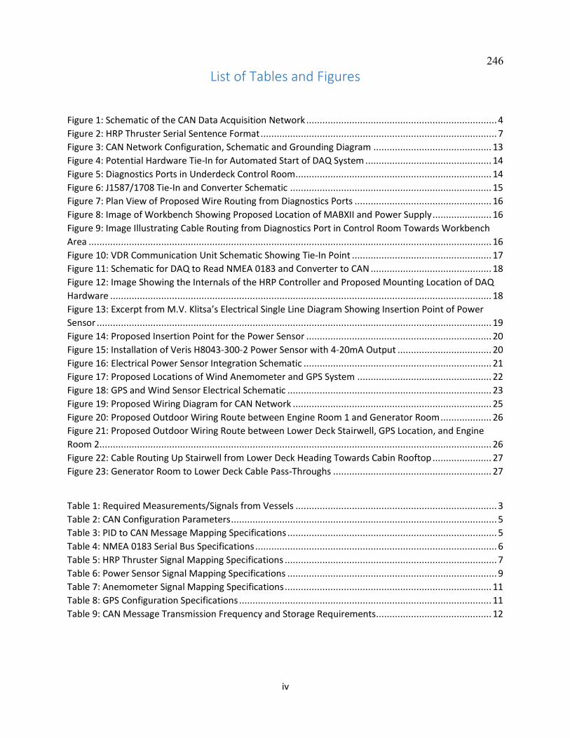
iv

List of Tables and Figures

Figure 1: Schematic of the CAN Data Acquisition Network ....................................................................... 4

Figure 2: HRP Thruster Serial Sentence Format ........................................................................................ 7

Figure 3: CAN Network Configuration, Schematic and Grounding Diagram ............................................ 13

Figure 4: Potential Hardware Tie-In for Automated Start of DAQ System ............................................... 14

Figure 5: Diagnostics Ports in Underdeck Control Room ......................................................................... 14

Figure 6: J1587/1708 Tie-In and Converter Schematic ........................................................................... 15

Figure 7: Plan View of Proposed Wire Routing from Diagnostics Ports ................................................... 16

Figure 8: Image of Workbench Showing Proposed Location of MABXII and Power Supply ...................... 16

Figure 9: Image Illustrating Cable Routing from Diagnostics Port in Control Room Towards Workbench

Area ...................................................................................................................................................... 16

Figure 10: VDR Communication Unit Schematic Showing Tie-In Point .................................................... 17

Figure 11: Schematic for DAQ to Read NMEA 0183 and Converter to CAN ............................................. 18

Figure 12: Image Showing the Internals of the HRP Controller and Proposed Mounting Location of DAQ

Hardware .............................................................................................................................................. 18

Figure 13: Excerpt from M.V. Klitsa’s Electrical Single Line Diagram Showing Insertion Point of Power

Sensor ................................................................................................................................................... 19

Figure 14: Proposed Insertion Point for the Power Sensor ..................................................................... 20

Figure 15: Installation of Veris H8043-300-2 Power Sensor with 4-20mA Output ................................... 20

Figure 16: Electrical Power Sensor Integration Schematic ...................................................................... 21

Figure 17: Proposed Locations of Wind Anemometer and GPS System .................................................. 22

Figure 18: GPS and Wind Sensor Electrical Schematic ............................................................................ 23

Figure 19: Proposed Wiring Diagram for CAN Network .......................................................................... 25

Figure 20: Proposed Outdoor Wiring Route between Engine Room 1 and Generator Room ................... 26

Figure 21: Proposed Outdoor Wiring Route between Lower Deck Stairwell, GPS Location, and Engine

Room 2 .................................................................................................................................................. 26

Figure 22: Cable Routing Up Stairwell from Lower Deck Heading Towards Cabin Rooftop ...................... 27

Figure 23: Generator Room to Lower Deck Cable Pass-Throughs ........................................................... 27

Table 1: Required Measurements/Signals from Vessels ........................................................................... 3

Table 2: CAN Configuration Parameters ................................................................................................... 5

Table 3: PID to CAN Message Mapping Specifications .............................................................................. 5

Table 4: NMEA 0183 Serial Bus Specifications .......................................................................................... 6

Table 5: HRP Thruster Signal Mapping Specifications ............................................................................... 7

Table 6: Power Sensor Signal Mapping Specifications .............................................................................. 9

Table 7: Anemometer Signal Mapping Specifications ............................................................................. 11

Table 8: GPS Configuration Specifications .............................................................................................. 11

Table 9: CAN Message Transmission Frequency and Storage Requirements ........................................... 12

246

1

Introduction UVic’s Marine Hybrid Power Systems Research group is currently under contract with Transport Canada

under the Clean Transportation Initiative to develop a set of modeling tools for the analysis of advanced

marine propulsion systems. The objective of this project is to develop a time-domain modeling and

simulation platform that is capable of accurately representing the ship motion, propulsion system, and

integrated power system dynamics. This model-based approach to propulsion system development has

seen wide success in hybrid and electric vehicles in the automotive industry. Despite its advantages in

achieving true design optimization, model based design has not been as well established in the marine

industry.

Traditionally, naval architects would design a ship based on a set of design requirements including

specification of contract speed, seakeeping metrics, environmental conditions, etc. Designers would

then seek to meet all these requirements through hull, powerplant, and propulsor selection. However,

studies have shown that many ships don’t operate at their original design point, often leading to poorer

system efficiency. As a result, there is a growing need for a “mission cycle” oriented approach to

propulsion analysis that can provide a true measure of system performance.

The present challenge is to develop a modeling tool that is capable of accurately predicting propulsive

load for the hybrid power system. In order to create a relatively simple case to test the effectiveness of

the tool for a ship both transit and maneuvering, a detailed data acquisition study of the BC Ferries M.V.

Klitsa will be conducted and compared to the results of the modeling platform. The data acquisition

(DAQ) will collect essential information from all power producing components on the ship including

main propulsive loads and electrical generation. In addition, the DAQ system attempts to capture the

oceanographic and environmental conditions for quantifying these external forces.

In order to validate the model, the DAQ will record the actuator position information from the azimuth

propellers to assess the effectiveness of the model in predicting maneuvering behaviour. Lastly, GPS

data will provide vessel speed and position data for validating output.

This document presents the integration and implementation details for the DAQ system to be installed

on the M.V. Klitsa. Prior to deploying the full system, the individual interfacing components will be

tested onboard the Kuper over the course of November 2014 while the ship is out of service. . The

Kuper has a similar propulsion system components, so the DAQ equipment will be compatible with both

vessels.

The plan outlined in this document comes as a result of collaboration with BC Ferries technicians and

the Senior Engineer of the Klitsa. This document serves as UVic’s proposed arrangement, but our group

remains open to suggestions or alternate configurations that will meet the study requirements.

247

2

Objectives The objective of this data acquisition study is to provide a validation test case for the hydrodynamic ship

dynamics modeling platform being developed at UVic. One of the major challenges in naval architecture

is developing an accurate representation of the variable propulsive loads that will be encountered on a

vessel throughout its lifecycle. A plant model of a ship must be able to accurately quantify the time-

domain loads for a given mission cycle and architecture. One of the core functionalities of this modeling

platform is to generate a mechanism by which propulsive system loads can be extracted using vessel

position and velocity data as inputs, as would be the case during the design phase.

Conversely, the tool can be deployed to evaluate performance through simulation of a specific

propulsion architecture. One can then evaluate different propulsors, engines, and generators under

various operating profiles and environmental conditions.

Given the functionality requirements of the hybrid propulsion modeling platform, this study seeks to

collect the necessary data to validate the core functionalities of the tool. BC Ferries has provided the

hull CAD file, design data, propeller performance curves, and sea trial that can be used to support the

validation process through all stages. The objective of the data acquisition study is to collect a complete

set of data which can serve as both the inputs and outputs for the ship model validation.

Using GPS information and the existing vessel architecture as inputs, the tool will be used to estimate

the propulsive system load at the propeller shaft. This will then be compared to the output of the main

diesel engines and will form the first validation check. Using the actuator thrust information as inputs

(includes propeller speed, torque, and azimuth angle), the position, heading, vessel speed can be

compared to that measured in the study. This will provide a measure of accuracy for the maneuvering

model.

Data Acquisition System Overview Conducting a data acquisition system on an operational vessel without a fully integrated communication

bus network is extraordinarily challenging. The system must be non-invasive and take all necessary

measures to ensure that the integrity of the onboard systems is maintained. Another complication

arises in planning the routing of cables between sensors. The hull is divided into four watertight sealed

compartments for safety. This implies that cable routing must be planned carefully to minimize, or

ideally eliminate the need for compartment cable pass-throughs.

The physical parameters of interest for the data acquisition study are presented in Table 1. To minimize

the amount of new equipment required, the goal is to access the existing serial buses wherever feasible.

These buses broadcast many of the physical measurements needed for the study; however, it requires

careful execution so as not to compromise the existing network. In some cases, new sensors have been

installed for practicality. Information on the sensors can be found in the electronic folder included with

this document.

The collection of all signals is done over a centralized CAN network that operates independently from

the other serial buses. Data is collected and stored on the Cross Chasm C5 GPS data logger which has a

removable flash storage card. To convert the serial bus data from the J1587/1708 and NMEA 0183

248

3

onboard communication buses, UVic’s system will incorporate microprocessor based converter units to

read the necessary signals and broadcast them over CAN. The schematic of the proposed system is

illustrated in Figure 1.

Table 1: Required Measurements/Signals from Vessels

Description Physical Parameter Transducer Signal Source

GPS Data Position (NED) Cross Chasm GPS Logger

Vessel Speed Cross Chasm GPS Logger

Engine 1 Data Engine Load J1587/J1708 Serial Bus




Engine 2 Data Engine Load J1587/J1708 Serial Bus




Azimuth Propeller 1 Azimuth Angle Position HRP VDR Serial Bus

Thruster Position Reference HRP VDR Serial Bus

Azimuth Propeller 2 Azimuth Angle Position HRP VDR Serial Bus

Thruster Position Reference HRP VDR Serial Bus

Electrical Generator Output

Voltage 3-Phases Veris H8043-0300-2 Power Sensor

Current 3-Phases Veris H8043-0300-2 Power Sensor

Wind Data Wind Speed Campbell Scientific 05103LK Wind Monitor

Direction Campbell Scientific 05103LK Wind Monitor

Two additional sensors will be introduced to the system for wind and electrical power sensing. A wind

anemometer vane-style unit shall be mounted above deck in a suitable location with restricted access.

This sensor will provide a measurement of wind and incident direction to allow for quantification of

wind resistance. The Campbell Scientific 05103LK anemometer will be used which provides two 4-20mA

signals for wind speed and direction, respectively, which are converted to a CAN message.

An external electrical power sensor will be introduced to provide a measure of the electrical load

demand over time. This sensor uses a 3-phase measurement with 3 split-core current transformers and

3 voltage leads. Like the anemometer, its output is a 4-20mA analog signal. Because there are two

onboard generators, the CT’s and potential leads need to be installed on the AC bus rather than on a

specific generator.

The DAQ system is to be configured to run autonomously such that it will not require any user input for

initialization or terminating. The goal is to set the system to operate over 2-3 weeks to obtain a varied

set of data which includes different driver patterns, and environmental conditions. UVic researchers

may need to checkup on the system every couple days, which will arranged in advance with the

engineer on shift. The general schematic for the data acquisition system showing the tie-in points to the

onboard systems is provided in the proceeding sections. Though the initial testing and verification of

the system will be conducted on the Kuper while it is out of service, this document will present

integration details specific to the M.V. Klitsa.

249

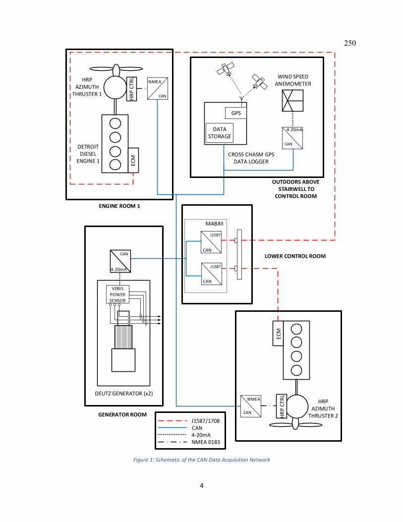
4

VERISPOWER SENSOR

DEUTZ GENERATOR (x2)

J1587

CAN

GPS

DATA STORAGE

CAN

4-20mA

CROSS CHASM GPSDATA LOGGER

HR

P C

TR

L

WIND SPEEDANEMOMETER

DETROIT DIESEL

ENGINE 1

EC

M

EC

M

LOWER CONTROL ROOM

HRP AZIMUTH

THRUSTER 1

HRP AZIMUTH

THRUSTER 2J1587/1708CAN4-20mANMEA 0183

HR

P C

TR

L

CAN

NMEA

J1587

CAN

CAN

4-20mA

ENGINE ROOM 1

OUTDOORS ABOVE STAIRWELL TO

CONTROL ROOM

MABXII

GENERATOR ROOM CAN

NMEA

Figure 1: Schematic of the CAN Data Acquisition Network

250

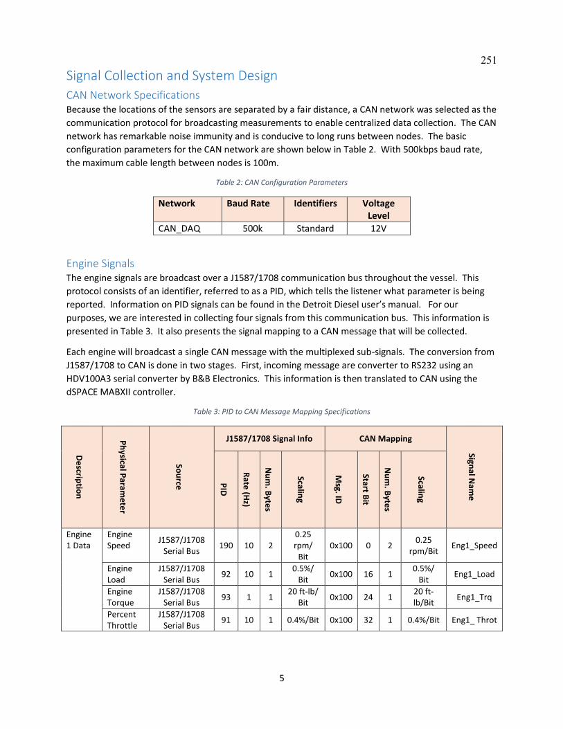
5

Signal Collection and System Design

CAN Network Specifications Because the locations of the sensors are separated by a fair distance, a CAN network was selected as the

communication protocol for broadcasting measurements to enable centralized data collection. The CAN

network has remarkable noise immunity and is conducive to long runs between nodes. The basic

configuration parameters for the CAN network are shown below in Table 2. With 500kbps baud rate,

the maximum cable length between nodes is 100m.

Table 2: CAN Configuration Parameters

Network Baud Rate Identifiers Voltage Level

CAN_DAQ 500k Standard 12V

Engine Signals The engine signals are broadcast over a J1587/1708 communication bus throughout the vessel. This

protocol consists of an identifier, referred to as a PID, which tells the listener what parameter is being

reported. Information on PID signals can be found in the Detroit Diesel user’s manual. For our

purposes, we are interested in collecting four signals from this communication bus. This information is

presented in Table 3. It also presents the signal mapping to a CAN message that will be collected.

Each engine will broadcast a single CAN message with the multiplexed sub-signals. The conversion from

J1587/1708 to CAN is done in two stages. First, incoming message are converter to RS232 using an

HDV100A3 serial converter by B&B Electronics. This information is then translated to CAN using the

dSPACE MABXII controller.

Table 3: PID to CAN Message Mapping Specifications

De

scriptio

n

Ph

ysical P

arame

ter

Sou

rce

J1587/1708 Signal Info CAN Mapping

Signa

l Nam

e

PID

Rate

(Hz)

Nu

m. B

ytes

Scaling

Msg. ID

Start Bit

Nu

m. B

ytes

Scaling

Engine 1 Data

Engine Speed

J1587/J1708 Serial Bus

190 10 2 0.25 rpm/

Bit 0x100 0 2

0.25 rpm/Bit

Eng1_Speed

Engine Load


92 10 1 0.5%/

Bit 0x100 16 1

0.5%/ Bit

Eng1_Load

Engine Torque


93 1 1 20 ft-lb/

Bit 0x100 24 1

20 ft-lb/Bit

Eng1_Trq

Percent Throttle


91 10 1 0.4%/Bit 0x100 32 1 0.4%/Bit Eng1_ Throt

251

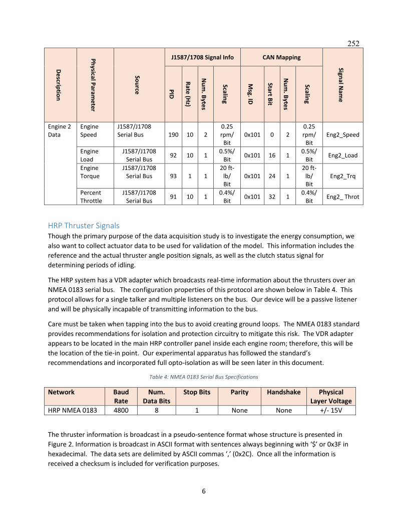
6

De

scriptio

n

Ph

ysical P

arame

ter

Sou

rce

J1587/1708 Signal Info CAN Mapping

Signa

l Nam

e

PID

Rate

(Hz)

Nu

m. B

ytes

Scaling

Msg. ID

Start Bit

Nu

m. B

ytes

Scaling

Engine 2 Data

Engine Speed

J1587/J1708 Serial Bus 190 10 2

0.25 rpm/

Bit 0x101 0 2

0.25 rpm/

Bit Eng2_Speed

Engine Load


92 10 1 0.5%/

Bit 0x101 16 1

0.5%/ Bit

Eng2_Load

Engine Torque

J1587/J1708 Serial Bus 93 1 1

20 ft-lb/ Bit

0x101 24 1 20 ft-

lb/ Bit

Eng2_Trq

Percent Throttle


91 10 1 0.4%/

Bit 0x101 32 1

0.4%/ Bit

Eng2_ Throt

HRP Thruster Signals Though the primary purpose of the data acquisition study is to investigate the energy consumption, we

also want to collect actuator data to be used for validation of the model. This information includes the

reference and the actual thruster angle position signals, as well as the clutch status signal for

determining periods of idling.

The HRP system has a VDR adapter which broadcasts real-time information about the thrusters over an

NMEA 0183 serial bus. The configuration properties of this protocol are shown below in Table 4. This

protocol allows for a single talker and multiple listeners on the bus. Our device will be a passive listener

and will be physically incapable of transmitting information to the bus.

Care must be taken when tapping into the bus to avoid creating ground loops. The NMEA 0183 standard

provides recommendations for isolation and protection circuitry to mitigate this risk. The VDR adapter

appears to be located in the main HRP controller panel inside each engine room; therefore, this will be

the location of the tie-in point. Our experimental apparatus has followed the standard’s

recommendations and incorporated full opto-isolation as will be seen later in this document.

Table 4: NMEA 0183 Serial Bus Specifications

Network Baud Rate

Num. Data Bits

Stop Bits Parity Handshake Physical Layer Voltage

HRP NMEA 0183 4800 8 1 None None +/- 15V

The thruster information is broadcast in a pseudo-sentence format whose structure is presented in

Figure 2. Information is broadcast in ASCII format with sentences always beginning with ‘$’ or 0x3F in

hexadecimal. The data sets are delimited by ASCII commas ‘,’ (0x2C). Once all the information is

received a checksum is included for verification purposes.

252

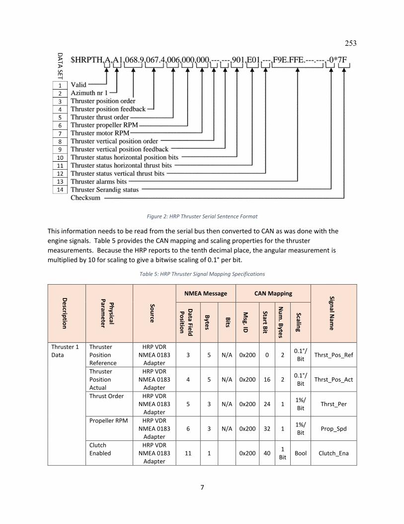
7

Figure 2: HRP Thruster Serial Sentence Format

This information needs to be read from the serial bus then converted to CAN as was done with the

engine signals. Table 5 provides the CAN mapping and scaling properties for the thruster

measurements. Because the HRP reports to the tenth decimal place, the angular measurement is

multiplied by 10 for scaling to give a bitwise scaling of 0.1° per bit.

Table 5: HRP Thruster Signal Mapping Specifications

De

scriptio

n

Ph

ysical

Param

ete

r

Sou

rce

NMEA Message CAN Mapping Signa

l Nam

e

Data Fie

ld

Po

sition

Byte

s

Bits

Msg. ID

Start Bit

Nu

m. B

ytes

Scaling

Thruster 1 Data

Thruster Position Reference

HRP VDR NMEA 0183

Adapter 3 5 N/A 0x200 0 2

0.1°/ Bit

Thrst_Pos_Ref

Thruster Position Actual

HRP VDR NMEA 0183

Adapter 4 5 N/A 0x200 16 2

0.1°/ Bit

Thrst_Pos_Act

Thrust Order HRP VDR NMEA 0183

Adapter 5 3 N/A 0x200 24 1

1%/ Bit

Thrst_Per

Propeller RPM HRP VDR NMEA 0183

Adapter 6 3 N/A 0x200 32 1

1%/ Bit

Prop_Spd

Clutch Enabled

HRP VDR NMEA 0183

Adapter 11 1 0x200 40

1 Bit

Bool Clutch_Ena

253

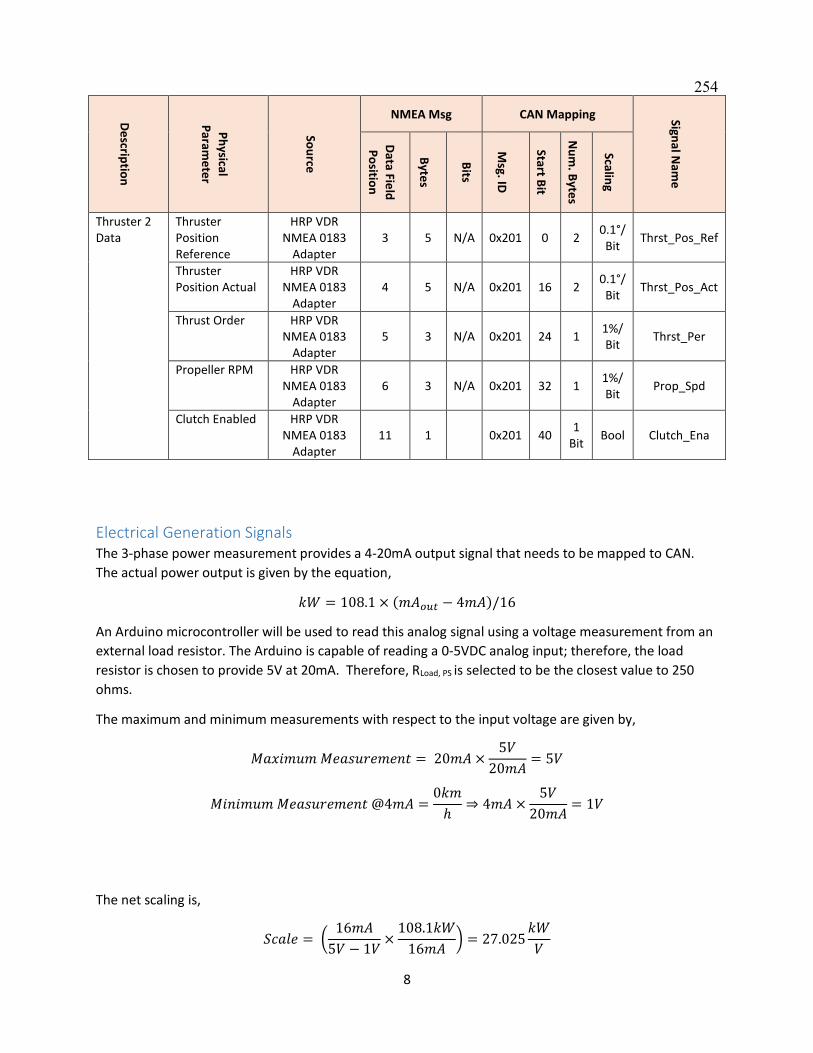
8

De

scriptio

n

Ph

ysical

Param

ete

r

Sou

rce

NMEA Msg CAN Mapping Signa

l Nam

e

Data Fie

ld

Po

sition

Byte

s

Bits

Msg. ID

Start Bit

Nu

m. B

ytes

Scaling

Thruster 2 Data

Thruster Position Reference

HRP VDR NMEA 0183

Adapter 3 5 N/A 0x201 0 2

0.1°/ Bit

Thrst_Pos_Ref

Thruster Position Actual

HRP VDR NMEA 0183

Adapter 4 5 N/A 0x201 16 2

0.1°/ Bit

Thrst_Pos_Act

Thrust Order HRP VDR NMEA 0183

Adapter 5 3 N/A 0x201 24 1

1%/ Bit

Thrst_Per

Propeller RPM HRP VDR NMEA 0183

Adapter 6 3 N/A 0x201 32 1

1%/ Bit

Prop_Spd

Clutch Enabled HRP VDR NMEA 0183

Adapter 11 1 0x201 40

1 Bit

Bool Clutch_Ena

Electrical Generation Signals The 3-phase power measurement provides a 4-20mA output signal that needs to be mapped to CAN.

The actual power output is given by the equation,

𝑘𝑊 = 108.1 × (𝑚𝐴𝑜𝑢𝑡 − 4𝑚𝐴)/16

An Arduino microcontroller will be used to read this analog signal using a voltage measurement from an

external load resistor. The Arduino is capable of reading a 0-5VDC analog input; therefore, the load

resistor is chosen to provide 5V at 20mA. Therefore, RLoad, PS is selected to be the closest value to 250

ohms.

The maximum and minimum measurements with respect to the input voltage are given by,

𝑀𝑎𝑥𝑖𝑚𝑢𝑚 𝑀𝑒𝑎𝑠𝑢𝑟𝑒𝑚𝑒𝑛𝑡 = 20𝑚𝐴 ×5𝑉

20𝑚𝐴= 5𝑉

𝑀𝑖𝑛𝑖𝑚𝑢𝑚 𝑀𝑒𝑎𝑠𝑢𝑟𝑒𝑚𝑒𝑛𝑡 @4𝑚𝐴 =0𝑘𝑚

ℎ⇒ 4𝑚𝐴 ×

5𝑉

20𝑚𝐴= 1𝑉

The net scaling is,

𝑆𝑐𝑎𝑙𝑒 = (16𝑚𝐴

5𝑉 − 1𝑉×

108.1𝑘𝑊

16𝑚𝐴) = 27.025

𝑘𝑊

𝑉

254

9

The measurement of power with respect to the input voltage then becomes,

𝑃𝑜𝑤𝑒𝑟 𝑂𝑢𝑡𝑝𝑢𝑡 = (27.025 𝑘𝑚/ℎ

𝑉⁄ × 𝑉𝑖𝑛) − 27.025𝑘𝑚/ℎ

The Arduino platform uses a 10bit ADC converter which provides 1024 discretized values for the analog

input signal which is good to 5V. Therefore, the resolution of the signal is given by,

𝐴𝐷𝐶 𝑅𝑒𝑠𝑜𝑙𝑢𝑡𝑖𝑜𝑛 = 5𝑉

1024= 0.00488

𝑉

𝐵𝑖𝑡

𝑆𝑖𝑔𝑛𝑎𝑙 𝑅𝑒𝑠𝑜𝑙𝑢𝑡𝑖𝑜𝑛 = 0.00488𝑉

𝐵𝑖𝑡× 27.025

𝑘𝑊

𝑉= 132

𝑊

𝐵𝑖𝑡

The CAN scaling will reflect the resolution of the ADC on the Arduino. These scaling variable will be

finalized once the circuit has been constructed; however, the CAN signal mapping is summarized below

in Table 6.

Table 6: Power Sensor Signal Mapping Specifications

Description Source

Tx Output CAN Mapping

Signal Name

Ou

tpu

t

Type

Ou

tpu

t

Scaling

CA

N

Msg. ID

Start Bit

Nu

m.

Bytes

CA

N M

sg. Scalin

g

3-φ Unbalanced Measurement

Veris Transducer

Analog 4-20mA 0x300 0 10 bit

132W/ Bit

Elec_Pwr_Act

Wind Anemometer Signals Similar to the power sensor, the wind anemometer provides two 4-20mA outputs for the physical

parameters representing wind speed and wind direction. Beginning with the wind speed measurement

system, the wind speed is calculated using the following equation:

𝑊𝑖𝑛𝑑 𝑆𝑝𝑒𝑒𝑑 = (12.5𝑘𝑚/ℎ

𝑚𝐴⁄ × 𝑚𝐴𝑜𝑢𝑡) − 50𝑘𝑚/ℎ

Here the scaling is 12.5km/h per milliamp of current. Again we want to structure the system such that

the maximum sensor output reflects the full voltage of the analog input. The maximum and minimum

measurement are then given by,


20𝑚𝐴= 5𝑉

𝑀𝑖𝑛𝑖𝑚𝑢𝑚 𝑀𝑒𝑎𝑠𝑢𝑟𝑒𝑚𝑒𝑛𝑡 = 4𝑚𝐴 ×5𝑉

20𝑚𝐴= 1𝑉

255

10

The physical measurement with respective to voltage is given by the scaling,


5𝑉 − 1𝑉×

12.5𝑘𝑚/ℎ

𝑚𝐴) = 50

𝑘𝑚/ℎ

𝑉

Therefore, the measurement with respect to ADC input voltage becomes,

𝑊𝑖𝑛𝑑 𝑆𝑝𝑒𝑒𝑑 = (50 𝑘𝑚/ℎ

𝑉⁄ × 𝑉𝑖𝑛) − 50𝑘𝑚/ℎ

The resolution of the ADC converter is the same as was presented in the power sensor; therefore, the

total signal resolution for wind speed is,

𝑊𝑖𝑛𝑑 𝑆𝑝𝑒𝑒𝑑 𝑅𝑒𝑠𝑜𝑙𝑢𝑡𝑖𝑜𝑛 = 0.00488𝑉

𝐵𝑖𝑡× 50

𝑘𝑚/ℎ

𝑉=

0.244𝑘𝑚/ℎ

𝐵𝑖𝑡=

0.68𝑚/𝑠

𝐵𝑖𝑡

The wind heading measurement is provided by a rotary weather-vane style system that uses a linear

potentiometer to determine angular position. The usable range for potentiometer is from 0° to 355°.

There is a five degree direction dead-band where the measurement will be ambiguous, thus this band

shall be placed in a direction with the least probable wind orientation. At first guess, the dead-band will

sit perpendicular to the length of the ship pointing towards the centre.

The wind direction measurement is given by,

𝑊𝑖𝑛𝑑 𝐷𝑖𝑟𝑒𝑐𝑡𝑖𝑜𝑛 = (22.5𝑑𝑒𝑔𝑟𝑒𝑒𝑠

𝑚𝐴⁄ × 𝑚𝐴𝑜𝑢𝑡) − 90 𝑑𝑒𝑔𝑟𝑒𝑒𝑠

Again designing the system to provide maximum rated voltage at full sensor output, the maximum and

minimum measurements are 5


20𝑚𝐴= 5𝑉

𝑀𝑖𝑛𝑖𝑚𝑢𝑚 𝑀𝑒𝑎𝑠𝑢𝑟𝑒𝑚𝑒𝑛𝑡 = 4𝑚𝐴 ×5𝑉

20𝑚𝐴= 1𝑉

The physical measurement with respective to voltage is given by the scaling,


5𝑉 − 1𝑉×

22.5𝑑𝑒𝑔𝑟𝑒𝑒𝑠

𝑚𝐴) = 90

𝑑𝑒𝑔𝑟𝑒𝑒𝑠

𝑉

The wind direction measurement with respect to ADC input voltage is given by,

𝑊𝑖𝑛𝑑 𝐷𝑖𝑟𝑒𝑐𝑡𝑖𝑜𝑛 = (90𝑑𝑒𝑔𝑟𝑒𝑒𝑠

𝑉⁄ × 𝑉𝑖𝑛) − 90 𝑑𝑒𝑔𝑟𝑒𝑒𝑠

Finally, the resolution can be determined as was done previously using,

𝑊𝑖𝑛𝑑 𝑆𝑝𝑒𝑒𝑑 𝑅𝑒𝑠𝑜𝑙𝑢𝑡𝑖𝑜𝑛 = 0.00488𝑉

𝐵𝑖𝑡× 90

𝑑𝑒𝑔𝑟𝑒𝑒𝑠

𝑉=

0.439𝑑𝑒𝑔𝑟𝑒𝑒𝑠

𝐵𝑖𝑡

The CAN message mapping and specification for these signals are provided below in Table 7.

256

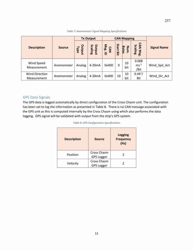
11

Table 7: Anemometer Signal Mapping Specifications

Description Source

Tx Output CAN Mapping

Signal Name

Ou

tpu

t

Type

Ou

tpu

t Scalin

g

CA

N

Msg. ID

Start Bit

Nu

m.

Bytes

CA

N M

sg.

Scaling

Wind Speed Measurement

Anemometer Analog 4-20mA 0x400 0 10bit

0.068 ms-1

/Bit Wind_Spd_Act

Wind Direction Measurement

Anemometer Analog 4-20mA 0x400 10 10bit

0.44°/ Bit

Wind_Dir_Act

GPS Data Signals The GPS data is logged automatically by direct configuration of the Cross Chasm unit. The configuration

has been set to log the information as presented in Table 8. There is no CAN message associated with

the GPS unit as this is computed internally by the Cross Chasm using which also performs the data

logging. GPS signal will be validated with output from the ship’s GPS system.

Table 8: GPS Configuration Specifications

Description Source Logging

Frequency (Hz)

Position Cross Chasm GPS Logger

2

Velocity Cross Chasm GPS Logger

2

257

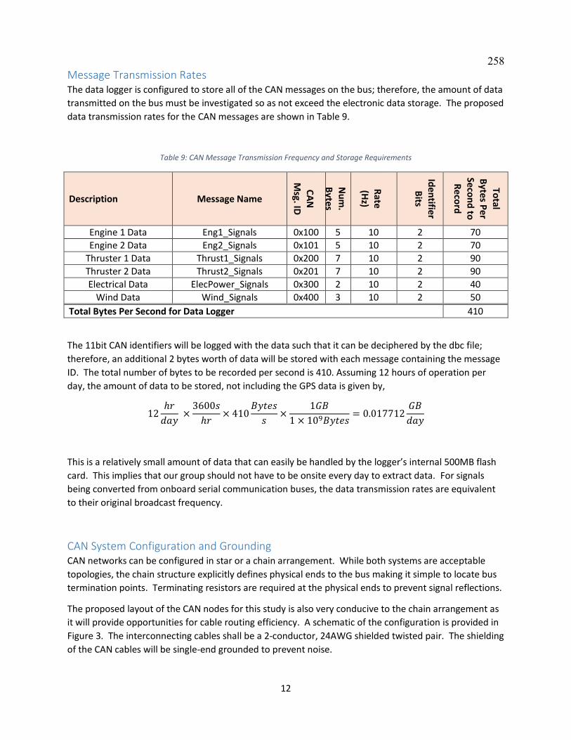
12

Message Transmission Rates The data logger is configured to store all of the CAN messages on the bus; therefore, the amount of data

transmitted on the bus must be investigated so as not exceed the electronic data storage. The proposed

data transmission rates for the CAN messages are shown in Table 9.

Table 9: CAN Message Transmission Frequency and Storage Requirements

Description Message Name

CA

N

Msg. ID

Nu

m.

Bytes

Rate

(Hz)

Iden

tifier

Bits

Total

Bytes P

er

Secon

d to

Re

cord

Engine 1 Data Eng1_Signals 0x100 5 10 2 70

Engine 2 Data Eng2_Signals 0x101 5 10 2 70

Thruster 1 Data Thrust1_Signals 0x200 7 10 2 90

Thruster 2 Data Thrust2_Signals 0x201 7 10 2 90

Electrical Data ElecPower_Signals 0x300 2 10 2 40

Wind Data Wind_Signals 0x400 3 10 2 50

Total Bytes Per Second for Data Logger 410

The 11bit CAN identifiers will be logged with the data such that it can be deciphered by the dbc file;

therefore, an additional 2 bytes worth of data will be stored with each message containing the message

ID. The total number of bytes to be recorded per second is 410. Assuming 12 hours of operation per

day, the amount of data to be stored, not including the GPS data is given by,

12ℎ𝑟

𝑑𝑎𝑦 ×

3600𝑠

ℎ𝑟× 410

𝐵𝑦𝑡𝑒𝑠

𝑠×

1𝐺𝐵

1 × 109𝐵𝑦𝑡𝑒𝑠= 0.017712

𝐺𝐵

𝑑𝑎𝑦

This is a relatively small amount of data that can easily be handled by the logger’s internal 500MB flash

card. This implies that our group should not have to be onsite every day to extract data. For signals

being converted from onboard serial communication buses, the data transmission rates are equivalent

to their original broadcast frequency.

CAN System Configuration and Grounding CAN networks can be configured in star or a chain arrangement. While both systems are acceptable

topologies, the chain structure explicitly defines physical ends to the bus making it simple to locate bus

termination points. Terminating resistors are required at the physical ends to prevent signal reflections.

The proposed layout of the CAN nodes for this study is also very conducive to the chain arrangement as

it will provide opportunities for cable routing efficiency. A schematic of the configuration is provided in

Figure 3. The interconnecting cables shall be a 2-conductor, 24AWG shielded twisted pair. The shielding

of the CAN cables will be single-end grounded to prevent noise.

258

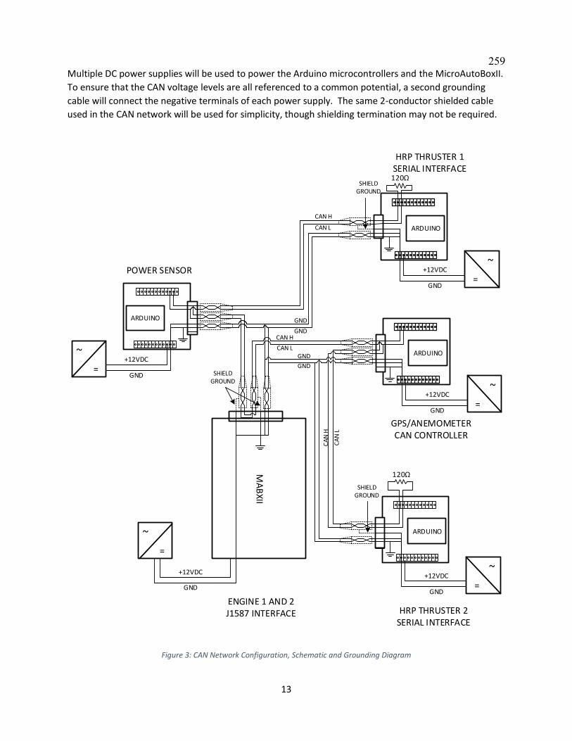
13

Multiple DC power supplies will be used to power the Arduino microcontrollers and the MicroAutoBoxII.

To ensure that the CAN voltage levels are all referenced to a common potential, a second grounding

cable will connect the negative terminals of each power supply. The same 2-conductor shielded cable

used in the CAN network will be used for simplicity, though shielding termination may not be required.

ARDUINO

=

~+12VDC

GND

HRP THRUSTER 1SERIAL INTERFACE

ARDUINO

=

~+12VDC

GND

POWER SENSOR

MA

BXII

=

~

GPS/ANEMOMETERCAN CONTROLLER

ARDUINO

=

~+12VDC

GND

ARDUINO

=

~+12VDC

GND

120Ω

CAN H

CAN L

GND

GNDCAN H

CAN LGND

GND

SHIELD GROUND

CA

N H

CA

N L

SHIELD GROUND

120Ω

SHIELD GROUND

+12VDC

GND

HRP THRUSTER 2SERIAL INTERFACE

ENGINE 1 AND 2J1587 INTERFACE

Figure 3: CAN Network Configuration, Schematic and Grounding Diagram

259

14

Automated Start/Stop Logging In order to conserve disk space and capture only the sensor information while the ship is running, it is

highly desirable that the data acquisition system have an automated hardware triggering signal. The

nodes of the CAN bus can be configured to begin transmitting after a specific message has been

received. Therefore, one of the controllers must have provisions to sense a digital hardware pin from

either the HRP thruster system or from the engine’s ECU.

One possible way to do this is to sense the voltage on the “Start Interlock” contactor provided by the

HRP system as shown in Figure 4. When this voltage level is logic high, then the system is stopped and

available for starting. When the logic is low, the engine is operating. After reviewing the HRP schematic,

we have not been able to determine where this terminal is located inside the main HRP controller unit

inside the engine room. This will require guidance from BC Ferries’ technicians to locate a suitable

hardware pin for this automated start/stop process.

Figure 4: Potential Hardware Tie-In for Automated Start of DAQ System

Integration Plan

Engine Signal Acquisition The engine signal acquisition will take place in the control room located underneath the main vehicle

deck. Signals from engines 1 and 2 are broadcast over J1587/1708 throughout the vessel, and two

diagnostics ports provide a convenient place to tap into the serial bus. The location of the two

diagnostics ports in the control room are shown in Figure 5.

Figure 5: Diagnostics Ports in Underdeck Control Room

260

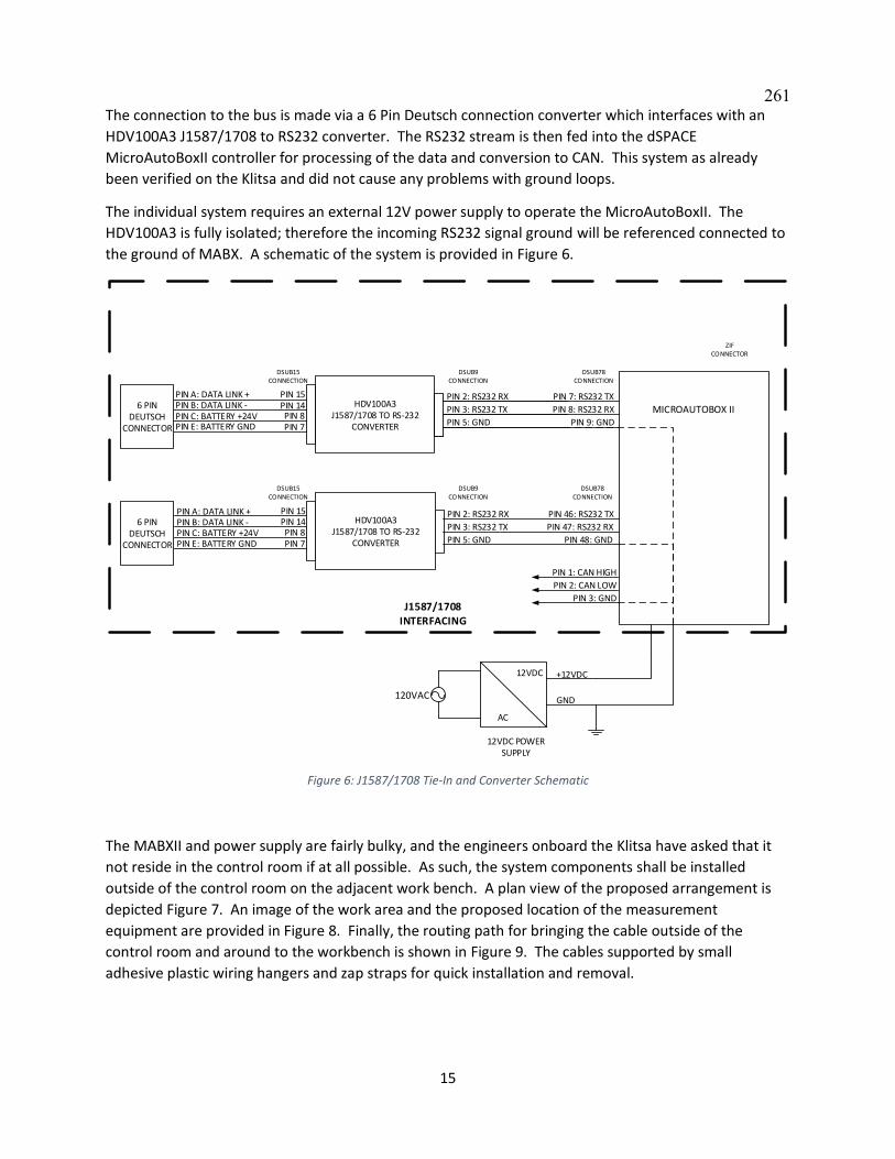
15

The connection to the bus is made via a 6 Pin Deutsch connection converter which interfaces with an

HDV100A3 J1587/1708 to RS232 converter. The RS232 stream is then fed into the dSPACE

MicroAutoBoxII controller for processing of the data and conversion to CAN. This system as already

been verified on the Klitsa and did not cause any problems with ground loops.

The individual system requires an external 12V power supply to operate the MicroAutoBoxII. The

HDV100A3 is fully isolated; therefore the incoming RS232 signal ground will be referenced connected to

the ground of MABX. A schematic of the system is provided in Figure 6.

6 PIN DEUTSCH

CONNECTOR

PIN A: DATA LINK +PIN B: DATA LINK -PIN C: BATTERY +24VPIN E: BATTERY GND

PIN 15PIN 14

PIN 7PIN 8

DSUB15CONNECTION

HDV100A3J1587/1708 TO RS-232

CONVERTER

MICROAUTOBOX II

DSUB9CONNECTION

PIN 2: RS232 RX

PIN 3: RS232 TX

PIN 5: GND

6 PIN DEUTSCH

CONNECTOR

PIN A: DATA LINK +PIN B: DATA LINK -PIN C: BATTERY +24VPIN E: BATTERY GND

PIN 15PIN 14

PIN 7PIN 8

DSUB15CONNECTION

HDV100A3J1587/1708 TO RS-232

CONVERTER

DSUB9CONNECTION

PIN 2: RS232 RX

PIN 3: RS232 TX

PIN 5: GND

PIN 7: RS232 TX

PIN 8: RS232 RX

PIN 9: GND

120VAC

AC

12VDC

PIN 46: RS232 TX

PIN 47: RS232 RX

PIN 48: GND

12VDC POWERSUPPLY

DSUB78CONNECTION

+12VDC

GND

PIN 1: CAN HIGH

PIN 2: CAN LOW

PIN 3: GND

DSUB78CONNECTION

ZIF CONNECTOR

J1587/1708INTERFACING

Figure 6: J1587/1708 Tie-In and Converter Schematic

The MABXII and power supply are fairly bulky, and the engineers onboard the Klitsa have asked that it

not reside in the control room if at all possible. As such, the system components shall be installed

outside of the control room on the adjacent work bench. A plan view of the proposed arrangement is

depicted Figure 7. An image of the work area and the proposed location of the measurement

equipment are provided in Figure 8. Finally, the routing path for bringing the cable outside of the

control room and around to the workbench is shown in Figure 9. The cables supported by small

adhesive plastic wiring hangers and zap straps for quick installation and removal.

261

16

WORKSHOPTABLE

UNDERDECKCONTROL ROOM

12VDCP.S.

MABXII

DIAGNOSTIC PORTS

120VAC

Figure 7: Plan View of Proposed Wire Routing from Diagnostics Ports

Figure 8: Image of Workbench Showing Proposed Location of

MABXII and Power Supply

Figure 9: Image Illustrating Cable Routing from Diagnostics

Port in Control Room Towards Workbench Area

262

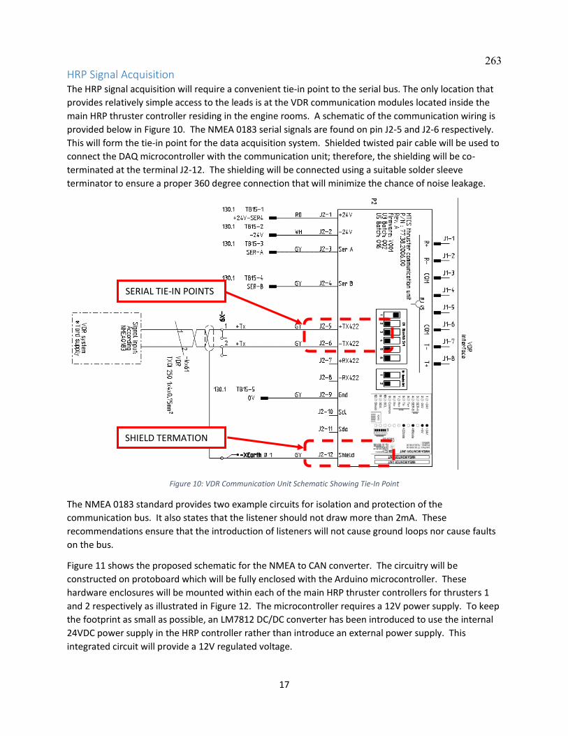
17

HRP Signal Acquisition The HRP signal acquisition will require a convenient tie-in point to the serial bus. The only location that

provides relatively simple access to the leads is at the VDR communication modules located inside the

main HRP thruster controller residing in the engine rooms. A schematic of the communication wiring is

provided below in Figure 10. The NMEA 0183 serial signals are found on pin J2-5 and J2-6 respectively.

This will form the tie-in point for the data acquisition system. Shielded twisted pair cable will be used to

connect the DAQ microcontroller with the communication unit; therefore, the shielding will be co-

terminated at the terminal J2-12. The shielding will be connected using a suitable solder sleeve

terminator to ensure a proper 360 degree connection that will minimize the chance of noise leakage.

Figure 10: VDR Communication Unit Schematic Showing Tie-In Point

The NMEA 0183 standard provides two example circuits for isolation and protection of the

communication bus. It also states that the listener should not draw more than 2mA. These

recommendations ensure that the introduction of listeners will not cause ground loops nor cause faults

on the bus.

Figure 11 shows the proposed schematic for the NMEA to CAN converter. The circuitry will be

constructed on protoboard which will be fully enclosed with the Arduino microcontroller. These

hardware enclosures will be mounted within each of the main HRP thruster controllers for thrusters 1

and 2 respectively as illustrated in Figure 12. The microcontroller requires a 12V power supply. To keep

the footprint as small as possible, an LM7812 DC/DC converter has been introduced to use the internal

24VDC power supply in the HRP controller rather than introduce an external power supply. This

integrated circuit will provide a 12V regulated voltage.

SERIAL TIE-IN POINTS

SHIELD TERMATION

263

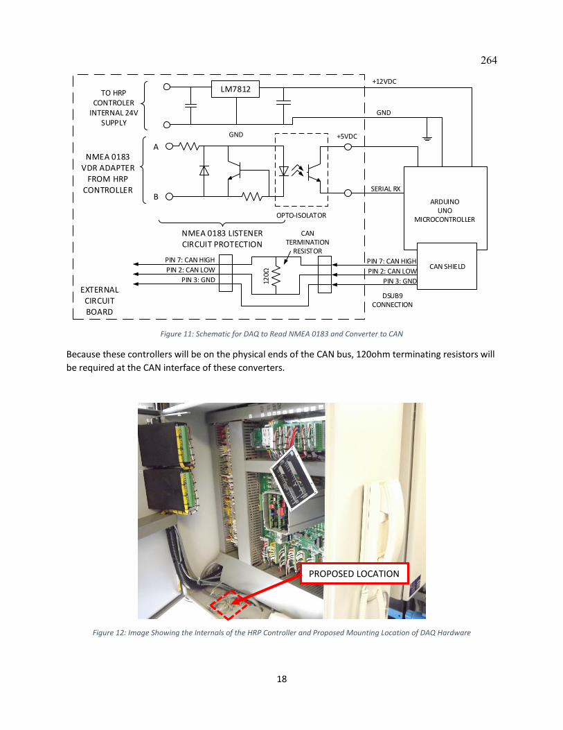
18

A

B

+5VDC

TO HRP CONTROLER

INTERNAL 24V SUPPLY

GND

SERIAL RX

ARDUINOUNO

MICROCONTROLLER

+12VDC

GND

OPTO-ISOLATOR

NMEA 0183 VDR ADAPTER

FROM HRP CONTROLLER

NMEA 0183 LISTENER CIRCUIT PROTECTION

CAN SHIELDPIN 7: CAN HIGH

PIN 2: CAN LOW

PIN 3: GND

DSUB9CONNECTION

PIN 7: CAN HIGH

PIN 2: CAN LOW

PIN 3: GND

EXTERNALCIRCUIT BOARD

120Ω

CANTERMINATION

RESISTOR

LM7812

Figure 11: Schematic for DAQ to Read NMEA 0183 and Converter to CAN

Because these controllers will be on the physical ends of the CAN bus, 120ohm terminating resistors will

be required at the CAN interface of these converters.

Figure 12: Image Showing the Internals of the HRP Controller and Proposed Mounting Location of DAQ Hardware

PROPOSED LOCATION

264

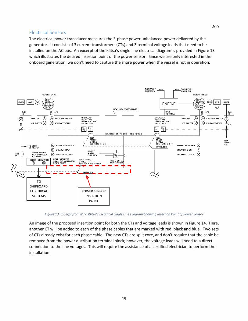
19

Electrical Sensors The electrical power transducer measures the 3-phase power unbalanced power delivered by the

generator. It consists of 3 current transformers (CTs) and 3 terminal voltage leads that need to be

installed on the AC bus. An excerpt of the Klitsa’s single line electrical diagram is provided in Figure 13

which illustrates the desired insertion point of the power sensor. Since we are only interested in the

onboard generation, we don’t need to capture the shore power when the vessel is not in operation.

Figure 13: Excerpt from M.V. Klitsa’s Electrical Single Line Diagram Showing Insertion Point of Power Sensor

An image of the proposed insertion point for both the CTs and voltage leads is shown in Figure 14. Here,

another CT will be added to each of the phase cables that are marked with red, black and blue. Two sets

of CTs already exist for each phase cable. The new CTs are split core, and don’t require that the cable be

removed from the power distribution terminal block; however, the voltage leads will need to a direct

connection to the line voltages. This will require the assistance of a certified electrician to perform the

installation.

TO

SHIPBOARD

ELECTRICAL

SYSTEMS

POWER SENSOR

INSERTION

POINT

265

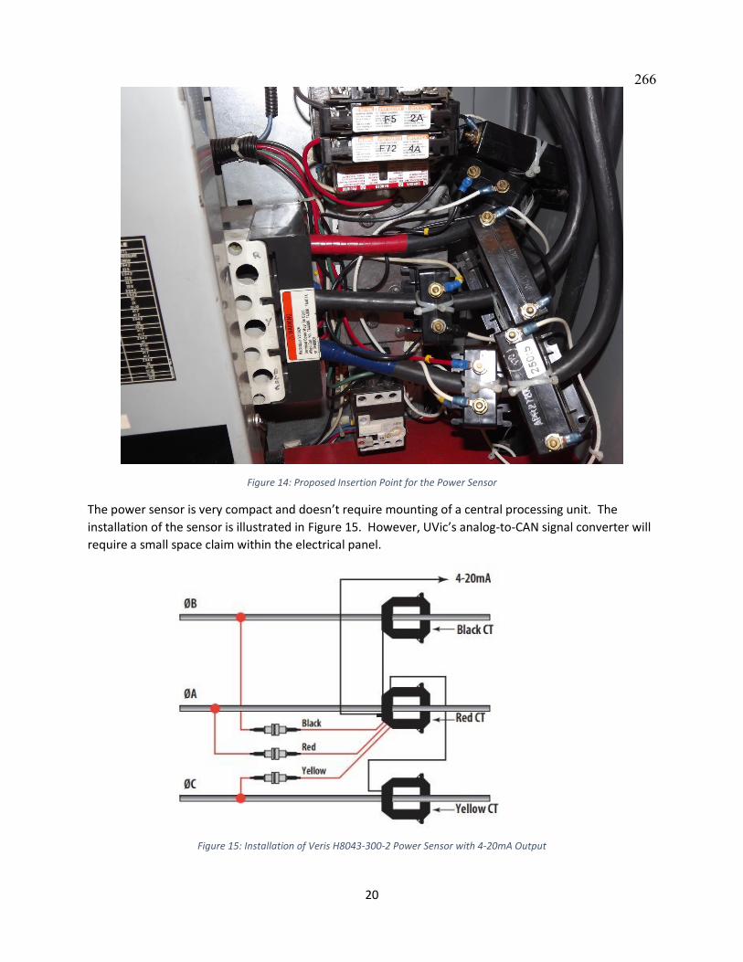
20

Figure 14: Proposed Insertion Point for the Power Sensor

The power sensor is very compact and doesn’t require mounting of a central processing unit. The

installation of the sensor is illustrated in Figure 15. However, UVic’s analog-to-CAN signal converter will

require a small space claim within the electrical panel.

Figure 15: Installation of Veris H8043-300-2 Power Sensor with 4-20mA Output

266

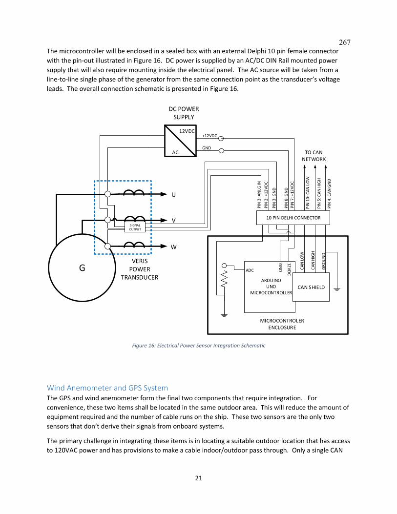
21

The microcontroller will be enclosed in a sealed box with an external Delphi 10 pin female connector

with the pin-out illustrated in Figure 16. DC power is supplied by an AC/DC DIN Rail mounted power

supply that will also require mounting inside the electrical panel. The AC source will be taken from a

line-to-line single phase of the generator from the same connection point as the transducer’s voltage

leads. The overall connection schematic is presented in Figure 16.

AC

12VDC

ARDUINOUNO

MICROCONTROLLER

+12VDC

CAN SHIELD

CA

N H

IGH

CA

N L

OW

G

SIGNALOUTPUT

12V

DC

GN

D

VERISPOWER

TRANSDUCER

U

V

W

GR

OU

ND

ADC

GND

MICROCONTROLER ENCLOSURE

DC POWER SUPPLY

TO CAN NETWORK

PIN

4: C

AN

GN

D

PIN

2: +

12V

DC

PIN

3: A

NLG

IN

PIN

7: +

12V

DC

PIN

5: C

AN

HIG

H

PIN

10

: CA

N L

OW

PIN

8: G

ND

PIN

3: G

ND

10 PIN DELHI CONNECTOR

Figure 16: Electrical Power Sensor Integration Schematic

Wind Anemometer and GPS System The GPS and wind anemometer form the final two components that require integration. For

convenience, these two items shall be located in the same outdoor area. This will reduce the amount of

equipment required and the number of cable runs on the ship. These two sensors are the only two

sensors that don’t derive their signals from onboard systems.

The primary challenge in integrating these items is in locating a suitable outdoor location that has access

to 120VAC power and has provisions to make a cable indoor/outdoor pass through. Only a single CAN

267

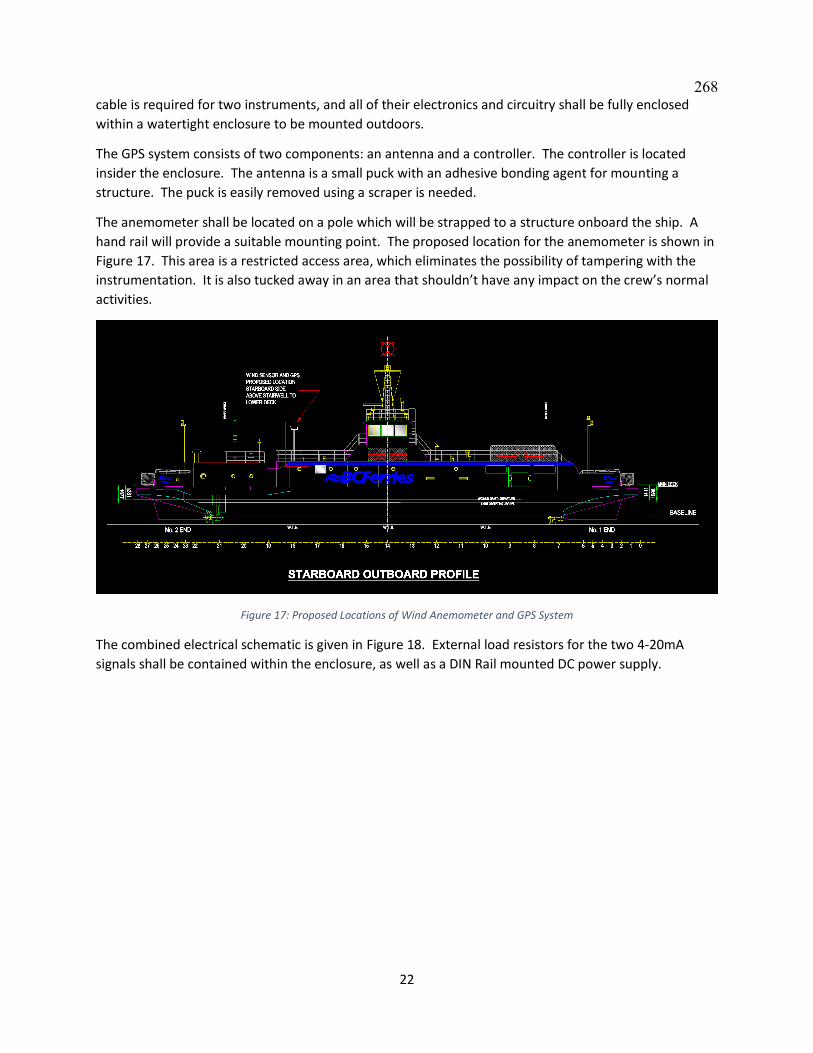
22

cable is required for two instruments, and all of their electronics and circuitry shall be fully enclosed

within a watertight enclosure to be mounted outdoors.

The GPS system consists of two components: an antenna and a controller. The controller is located

insider the enclosure. The antenna is a small puck with an adhesive bonding agent for mounting a

structure. The puck is easily removed using a scraper is needed.

The anemometer shall be located on a pole which will be strapped to a structure onboard the ship. A

hand rail will provide a suitable mounting point. The proposed location for the anemometer is shown in

Figure 17. This area is a restricted access area, which eliminates the possibility of tampering with the

instrumentation. It is also tucked away in an area that shouldn’t have any impact on the crew’s normal

activities.

Figure 17: Proposed Locations of Wind Anemometer and GPS System

The combined electrical schematic is given in Figure 18. External load resistors for the two 4-20mA

signals shall be contained within the enclosure, as well as a DIN Rail mounted DC power supply.

268

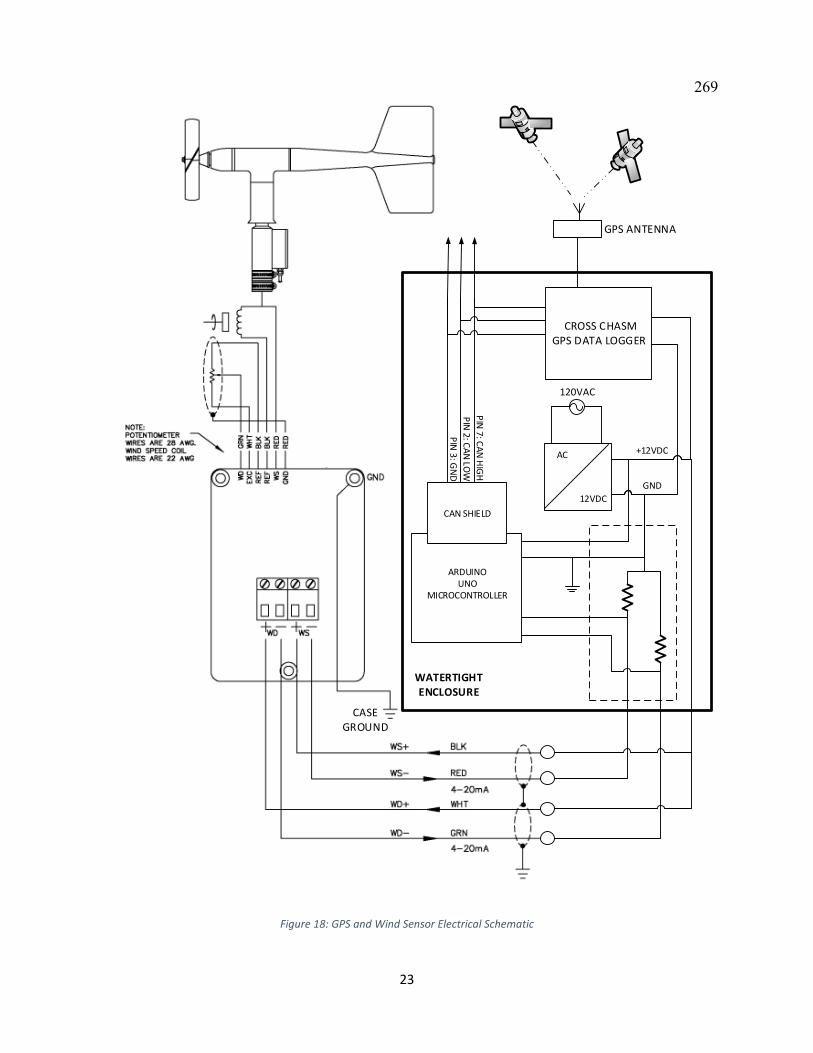
23

120VAC

AC

12VDC

ARDUINOUNO

MICROCONTROLLER

CAN SHIELD

PIN

7: CA

N H

IGH

PIN

2: CA

N LO

W

PIN

3: GN

D

+12VDC

GND

CROSS CHASMGPS DATA LOGGER

GPS ANTENNA

CASE GROUND

WATERTIGHTENCLOSURE

Figure 18: GPS and Wind Sensor Electrical Schematic

269

24

CAN Network Cable Routing and Grounding To physically connect the CAN nodes, it will be necessary to introduce external cables onboard the ship.

This is one of the primary challenges that UVic researchers have encountered in developing this plan.

The goal is to introduce these cables in such a way that it will not impact crew operations, nor passenger

amenities.

The ship’s hull is divided into four sealed compartments. Though these compartments do have

provisions for cable pass-throughs, utilizing these passage ways would require a re-sealing procedure

that is highly undesirable. Therefore, the proposed wire routing herein attempts to avoid crossing

sealed compartments underdeck. The design of the data acquisition system attempted to keep as much

instrumentation in the compartment containing the underdeck control room. Wherever possible, the

wiring is run underdeck to minimize the chance of cable damage.

The preliminary wire routing plan is presented in Figure 19. This illustration shows the desired pass-

through locations and provides the most desirable routing from our perspective. To minimize the risk of

crushing the cable on the main vehicle deck, UVic researchers would like to route cable outdoors on the

upper deck. Outdoor cable routing has been assumed to be the most practical approach whenever the

cable must cross sealed hull compartments. The cable can be tucked along the base of handrails and

secured so that it does not pose any tripping hazards.

The images of the proposed outdoor wiring are shown in Figure 20 and Figure 21. An image of the

proposed cable path to pass through the lower deck to the main vehicle deck is shown in Figure 22.

Existing cable pass-throughs for the generator room to the lower deck is presented in Figure 23.

Note it may be more convenient to run the cable underdeck from the GPS/Anemometer to the Engine

Room 2; however, it is currently unknown whether that would require a cable pass through across a

sealed compartment. Because of the daisy-chain style arrangement of the CAN network combined with

the outdoor location of the GPS/Anemometer, it makes more physical sense to make the final run

outdoors provided that a suitable pass-through can be supplied into the engine room from the roof.

Our group will require the guidance of the onboard engineers and technicians to provide input on the

best possible routing paths. This is probably the most logistically difficult portion of the data acquisition

experiment, so we are completely open to alternate wiring configurations provided that they meet our

requirements.

270

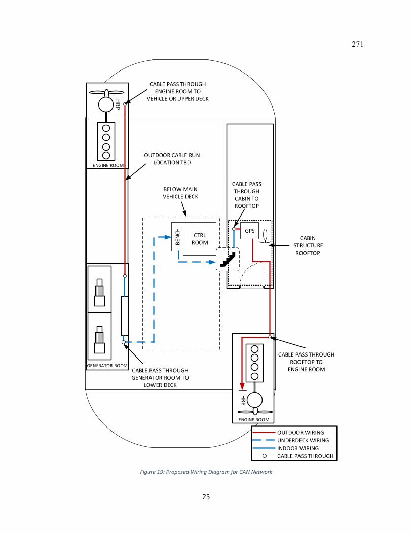
25

HR

P

CTRLROOMB

ENCH GPS

HR

P

BELOW MAINVEHICLE DECK

CABLE PASS THROUGHGENERATOR ROOM TO

LOWER DECK

CABLE PASS THROUGHENGINE ROOM TO

VEHICLE OR UPPER DECK

OUTDOOR CABLE RUNLOCATION TBD

CABIN STRUCTURE

ROOFTOP

CABLE PASS THROUGHCABIN TOROOFTOP

CABLE PASS THROUGHROOFTOP TO

ENGINE ROOM

OUTDOOR WIRING

UNDERDECK WIRING

INDOOR WIRING

CABLE PASS THROUGH

ENGINE ROOM

ENGINE ROOM

GENERATOR ROOM

Figure 19: Proposed Wiring Diagram for CAN Network

271

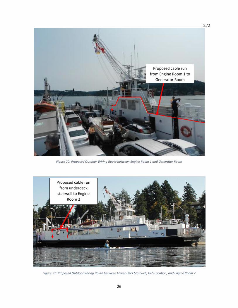
26

Figure 20: Proposed Outdoor Wiring Route between Engine Room 1 and Generator Room

Figure 21: Proposed Outdoor Wiring Route between Lower Deck Stairwell, GPS Location, and Engine Room 2

Proposed cable run

from Engine Room 1 to

Generator Room

Proposed cable run

from underdeck

stairwell to Engine

Room 2

272

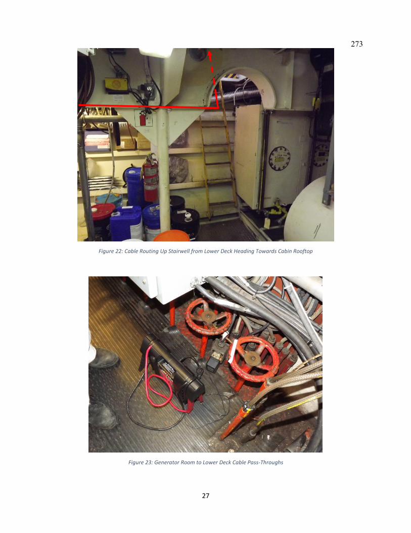
27

Figure 22: Cable Routing Up Stairwell from Lower Deck Heading Towards Cabin Rooftop

Figure 23: Generator Room to Lower Deck Cable Pass-Throughs

273

28

BC Ferries Installation Support

UVic’s research group will require various levels of support from BC Ferries throughout the planning and

execution of the study. The integration plan presented in the in previous sections sought to resolve the

majority of the installation details from studying the schematics; however, there are still some

unanswered questions regarding tie-in points and cable routing which will require further consultation

with onboard crew as well as the BC Ferries technicians. This will need to be done onsite after this

document has been reviewed.

The installation of the entire system shall be performed over the course of two days. The following

sections provide a high level description of the activities to be completed on each day. The goal is to

perform as much of the installation during normal work hours; however, some afterhours work will be

required when the connections to the serial bus are made while the ship is not in operation.

Day 1 On the first day, the team will arrive at first sailing and begin routing of the cables that will connect the

CAN nodes. This will be done with the help of the crew’s engineer who will provide both guidance and

assistance for the cable routing, and identifying suitable pass-throughs. The team will likely need to

access restricted areas of the ship, but the goal is to have no impact on the sailing schedule and the

crew’s daily operations.

The anemometer and the GPS system will be mounted and installed over the course of the day. During

the mid-day layover, the team will make the cable pass-throughs from the electrical room down to the

lower deck. Furthermore, a certified electrician shall be onsite to perform the installation of a power

sensor, which shouldn’t take more than 15 minutes. The duration of the day will be spent completing

the underdeck wiring. The J1587/1708 connections has already demonstrated that it poses no threat to

the integrity of the system, so it will be completed on Day 1.

Day 2 In the morning of Day 2, all remaining wiring shall be finalized, installed, and secured. The team will

spend the morning verifying connections, testing the CAN communication, and checking the

instrumentation prior to being hooked up. A BC Ferries technician shall arrive onsite after the final

sailing is complete. The team will then work with the technician to make all necessary communication

bus and electrical connections for the HRP thrusters and hardware enable pin for the automated start.

An engineer will also be required on the ship to assist in this process, and verify that the ship’s

functionality remains intact after the installation. With sufficient planning, this process should be

completed within two hours.

System Removal Once the DAQ system has collected all of the necessary data, the instrumentation will be removed in a

single day. An electrician will be required at mid-day layover to remove the power sensor and verify the

electrical connections, and a BC Ferries electrical technician will be required afterhours to disconnect

the serial bus tie-in lines.

274

DAQ Installation Photos

A-1

Figure A-1: J1587/1708 Engine Bus Connection in Control Room

Figure A-2: RS232/CAN Isolated Converter System

275

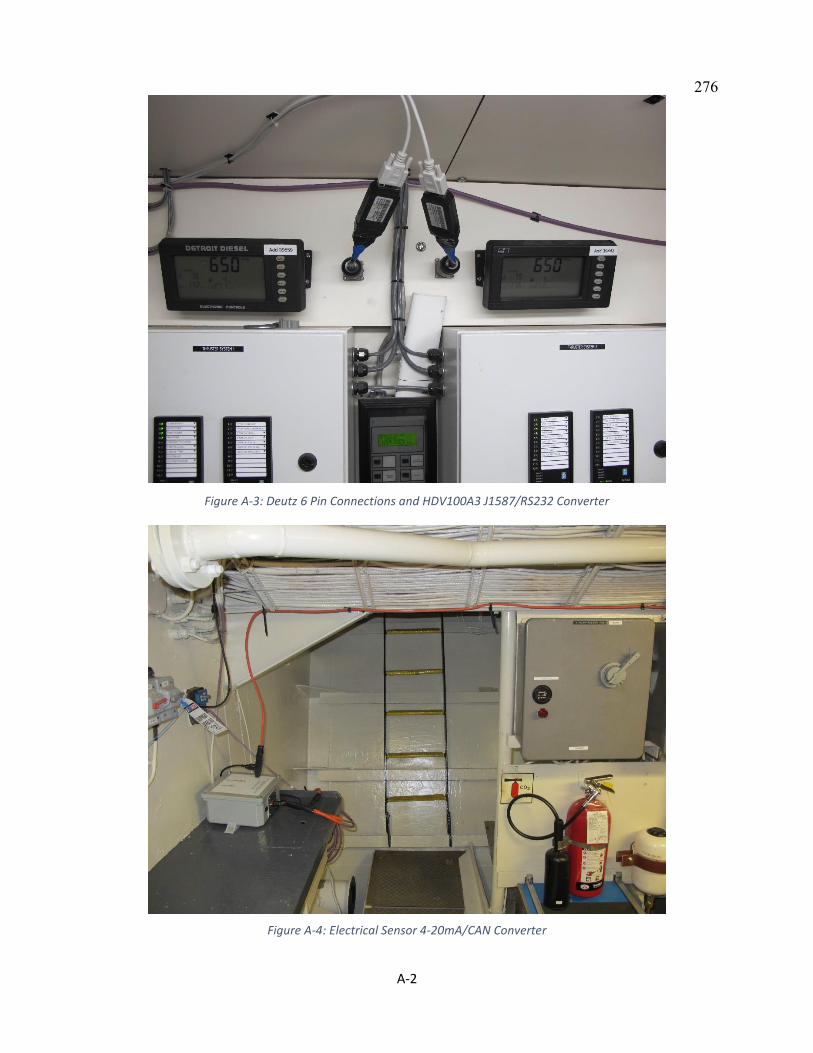
A-2

Figure A-3: Deutz 6 Pin Connections and HDV100A3 J1587/RS232 Converter

Figure A-4: Electrical Sensor 4-20mA/CAN Converter

276

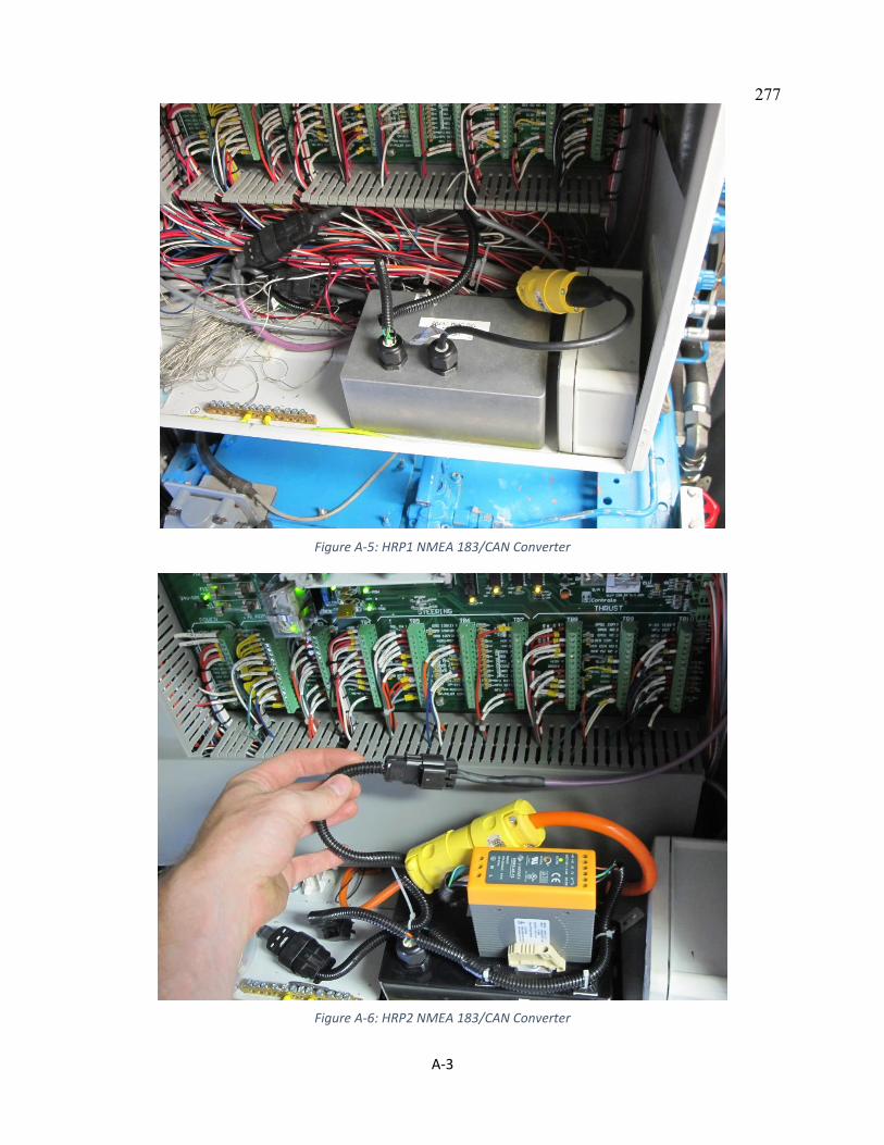
A-3

Figure A-5: HRP1 NMEA 183/CAN Converter

Figure A-6: HRP2 NMEA 183/CAN Converter

277

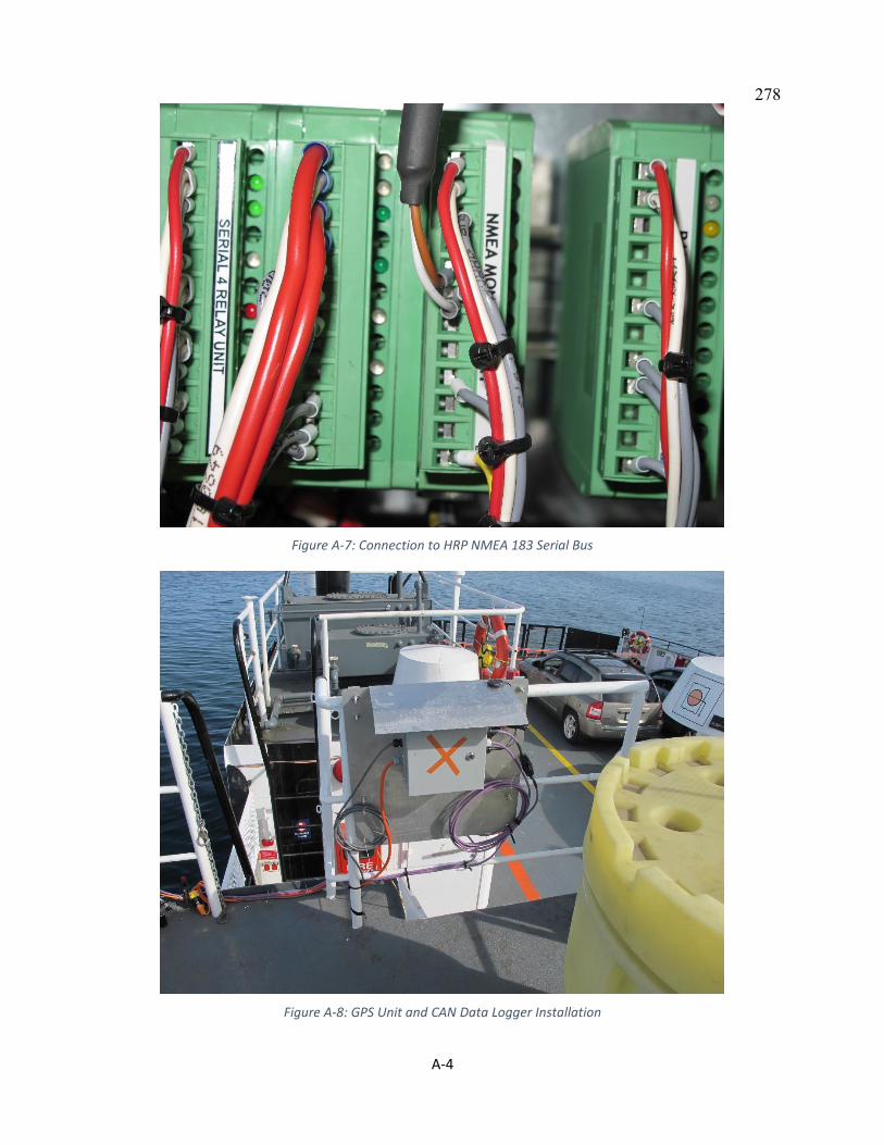
A-4

Figure A-7: Connection to HRP NMEA 183 Serial Bus

Figure A-8: GPS Unit and CAN Data Logger Installation

278

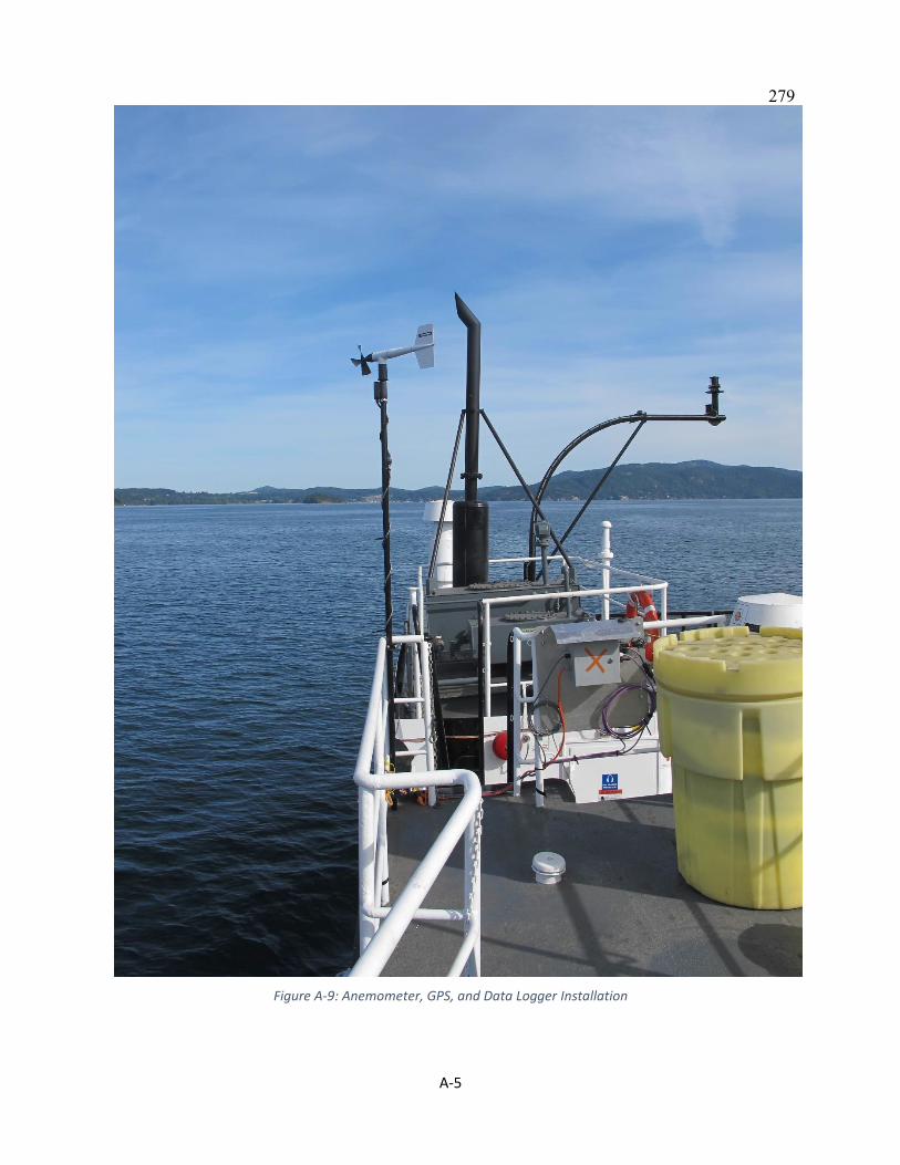
A-5

Figure A-9: Anemometer, GPS, and Data Logger Installation

279

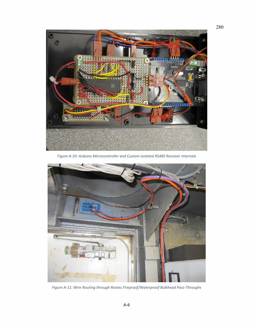
A-6

Figure A-10: Arduino Microcontroller and Custom Isolated RS485 Receiver Internals

Figure A-11: Wire Routing through Roxtec Fireproof/Waterproof Bulkhead Pass-Throughs

280

281

Appendix B – Derivation of DC/DC Converter Control Law

Beginning with the small-signal approximation equations developed in Chung, this

appendix verifies that the desired control law can be implemented. The small signal

equations presented in Table 21 are reintroduced here in the table below.

Buck Mode Boost Mode

Inductor

Balance

𝐿𝑑𝑖𝐿𝑑𝑡=1

𝑛𝐷𝑣𝑑𝑐 +

1

𝑛𝑉𝐷𝐶 − 𝑣𝑏𝑎𝑡𝑡

( B - 1 )

𝐿𝑑𝑖𝐿𝑑𝑡= 𝑣𝑏𝑎𝑡𝑡 −

𝐷′

𝑛𝑣𝑑𝑐 +

1

𝑛𝑉𝐷𝐶

( B - 2 )

Output Current 𝐶1𝑑𝑣𝑏𝑎𝑡𝑡𝑑𝑡

= 𝑖𝐿 −𝑣𝑏𝑎𝑡𝑡𝑅1

( B - 3 )


=𝐷′

𝑛𝑖𝐿 −

1

𝑛𝐼𝐿 −

𝑣𝑑𝑐𝑅2

( B - 4 )

Input Current 𝐶2𝑑𝑣𝑑𝑐𝑑𝑡

≈ 𝑖𝑑𝑐 − 𝑛𝐼𝐿 − 𝑛𝐷𝑖𝐿

( B - 5 )

𝐶1𝑑𝑣𝑏𝑎𝑡𝑡𝑑𝑡

≈ 𝑖𝑏𝑎𝑡𝑡 − 𝑖𝐿

( B - 6 )

Transformer

Current

𝑖𝑠 =1

𝑛𝑖𝐿

( B - 7 )

𝑖𝑠 =1

𝑛𝑖𝐿𝐷′

( B - 8 )

Considering first buck mode, we need to develop some insight into the physical system

behaviour to develop the control equations. In buck mode, the system is absorbing power

by charging the ESS. The bus voltage (HV) is still to be regulated by the DC/DC

converter, so current can be sourced from the PMSM drive system by commanding

regeneration torque. The ESS side voltage (LV) is set by the battery bank; therefore,

current must be the control variable on the LV side to balance the power.

282

We begin by defining the time-domain inputs and outputs of the system. It is

convenient to write the system in state space format for checking controllability. The

states of the small-signal equations for buck mode are given by,

Let, 𝑥1 = 𝑖𝐿 ( B - 9 ) ⇒ 1 =𝑑𝑖𝐿𝑑𝑡

( B - 10 )

𝑥2 = 𝑣𝑏𝑎𝑡𝑡 ( B - 11 ) ⇒ 2 =𝑑𝑣𝑏𝑎𝑡𝑡𝑑𝑡

( B - 12 )

𝑥3 = 𝑣𝑑𝑐 ( B - 13 ) ⇒ 3 =𝑑𝑣𝑑𝑐𝑑𝑡

( B - 14 )

We define the inputs to the system as duty cycle d and input current 𝑖𝑑𝑐. In state vector

form, we can write input and output vectors as

Input Vector Output Vector

𝒖 = [𝑖𝑑𝑐] ( B - 15 ) 𝑦 = 𝑥3 ( B - 16 )

Now, the state space representation for buck mode can be written as,

[123

] = [

0 −1 𝐿⁄ 𝐷 𝐿𝑛⁄

1 𝐶1⁄ −1 𝑅1𝐶1⁄ 0

−𝑛𝐷 𝐶2⁄ 0 0]

⏟ 𝐴

[

𝑥1𝑥2𝑥3] + [

𝑉𝐷𝐶 𝐿𝑛⁄ 00 0

−𝑛𝐷 𝐶2⁄ 0]

⏟ 𝐵

[𝑖𝑑𝑐]

( B - 17 )

[𝑦1] = [0 0 1]⏟ 𝐶

[

𝑥1𝑥2𝑥3] + [0 0]⏟

𝐷

[𝑖𝑑𝑐] ( B - 18 )

The controllability matrix is formulated as follows:

𝑅 = [𝐴 𝐴𝐵 𝐴2𝐵 ⋯ 𝐴𝑚−1𝐵] ( B - 19 )

The system is considered controllable if the matrix R is of rank m. Matlab’s function

ctrb() builds the controllability matrix from state space system object. The function rank

283

determines the rank of the system; therefore, if rank(A) and rank(R) are the equal, then

the system is controllable. A Matlab script and its subsequent results for numerical

examples provided in Chung et al. [25] and Zahedi et al. [26] are presented after

derivation of the boost mode.

We can develop a similar expressions for the converter is boost mode. In this mode of

operation, the converter takes voltage input from the battery terminals and manipulates

the duty cycle d for switches on the current fed side to regulate the DC bus voltage. If we

define the states as,

Let, 𝑥1 = 𝑖𝐿 ( B - 20 ) ⇒ 1 =𝑑𝑖𝐿𝑑𝑡

( B - 21 )

𝑥2 = 𝑣𝑑𝑐 ( B - 22 ) ⇒ 2 =𝑑𝑣𝑑𝑐𝑑𝑡

( B - 23 )

We define the inputs to the system as duty cycle d and battery’s input voltage 𝑣𝑏𝑎𝑡𝑡. In

state vector form,

Input Vector Output Vector

𝒖 = [

𝑣𝑏𝑎𝑡𝑡] ( B - 24 ) 𝑦 = 𝑥2 ( B - 25 )

Then the state space representation for boost mode can be written as,

[12] = [

0 −𝐷′ 𝐿𝑛⁄

𝐷′ 𝑛𝐶2⁄ −1 𝑅2𝐶2⁄]

⏟ 𝐴

[𝑥1𝑥2] + [

𝑉𝑑𝑐 𝐿𝑛⁄ 1 𝐿⁄

−𝐼𝐿 𝑛⁄ 𝐶2 0]

⏟ 𝐵

[

𝑣𝑏𝑎𝑡𝑡]

( B - 26 )

[𝑦1] = [0 1]⏟ [𝑥1𝑥2]

𝐶

+ [0 0]⏟ 𝐷

[

𝑣𝑏𝑎𝑡𝑡] ( B - 27 )

284

Returning back to buck mode, the transfer function governing the voltage regulation in

can be developed by taking the Laplace transform of equation ( B - 1 ) for inductor

balance to yield the result,

𝑠𝐿𝑖𝐿(𝑠) =1

𝑛𝐷𝑣𝑑𝑐(𝑠) +

1

𝑛𝑉𝐷𝐶(𝑠) − 𝑣𝑏𝑎𝑡𝑡(𝑠)

( B - 28 )

The input and output current relationships, Equation ( B - 5 ) and Equation ( B - 3 ),

can be transformed, rearranged and substituted into the equation above to develop the

control law as shown below.

Input Current (Buck): 𝑠𝐶1𝑣𝑏𝑎𝑡𝑡(𝑠) = 𝑖𝐿(𝑠) −𝑣𝑏𝑎𝑡𝑡(𝑠)

𝑅1 ( B - 29 )

Output Current (Buck): 𝑠𝐶2𝑣𝑑𝑐(𝑠) = 𝑖𝑑𝑐(𝑠) − 𝑛𝐼𝐿(𝑠) − 𝑛𝐷𝑖𝐿(𝑠) ( B - 30 )

Rearranging Equation ( B - 30 ) to isolate the averaged inductor current we get,

𝑖𝐿(𝑠) =1

𝑛𝐷[𝑖𝑑𝑐(𝑠) − 𝑠𝐶2𝑣𝑑𝑐(𝑠) − 𝑛𝐼𝐿(𝑠)] ( B - 31 )

We will use the above result to substitute into the inductor balance equation to get,

𝑠𝐿

𝑛𝐷[𝑖𝑑𝑐(𝑠) − 𝑠𝐶2𝑣𝑑𝑐(𝑠) − 𝑛𝐼𝐿(𝑠)]

=1


1


( B - 32 )

Expanding we get,

−𝑠2𝐿𝐶2𝑛𝐷

𝑣𝑑𝑐(𝑠) +𝑠𝐿

𝑛𝐷𝑖𝑑𝑐(𝑠) −

𝑠𝐿𝐼𝐿𝐷(𝑠)

=1


1


( B - 33 )

285

Grouping like-terms yields,

− [𝑠𝐿𝐼𝐿𝐷

+1

𝑛𝑉𝐷𝐶] (𝑠)

= [𝑠2𝐿𝐶2𝑛𝐷

+1

𝑛𝐷] 𝑣𝑑𝑐(𝑠) − 𝑣𝑏𝑎𝑡𝑡(𝑠)⏟

𝐷𝑖𝑠𝑡𝑢𝑟𝑏𝑎𝑛𝑐𝑒

−𝑠𝐿

𝑛𝐷𝑖𝑑𝑐(𝑠)⏟

𝐷𝑖𝑠𝑡𝑢𝑟𝑏𝑎𝑛𝑐𝑒

( B - 34 )

Finally we arrive at the control transfer function for controlling DC bus voltage using

duty cycle manipulation of the voltage-fed converter.

𝐺𝑣𝑑𝑐∙𝑑(𝑠) =𝑣𝑑𝑐(𝑠)

(𝑠)= −

𝑠𝐿𝐼𝐿𝐷 +

1𝑛 𝑉𝐷𝐶

𝑠2𝐿𝐶2𝑛𝐷 +

1𝑛𝐷

=−(𝑠𝑛𝐿𝐼𝐿 + 𝐷𝑉𝐷𝐶)

𝑠2𝐿𝐶2 + 𝐷2 ( B - 35 )

Similarly, the transfer function governing the voltage regulation in boost mode can be

developed by taking the Laplace transform of the average value equation for inductor

balance, Equation ( B - 2 ), to yield the result,

𝑠𝐿𝑖𝐿(𝑠) = 𝑣𝑏𝑎𝑡𝑡(𝑠) −𝐷′

𝑛𝑣𝑑𝑐(𝑠) +

1

𝑛𝑉𝐷𝐶(𝑠) ( B - 36 )

Again, we are using the output current balance equation to develop the control transfer

function. Taking the Laplace transform of the output current relationship defined by

Equation ( B - 4 ), we get

𝑠𝐶2𝑣𝑑𝑐(s) =𝐷′

𝑛𝑖𝐿(𝑠) −

1

𝑛𝐼𝐿(𝑠) −

𝑣𝑑𝑐(𝑠)

𝑅2 ( B - 37 )

The equation can be rearranged to isolated averaged inductor current,

𝑖𝐿(𝑠) =𝑛

𝐷′[(𝑠𝐶2 +

1

𝑅2) 𝑣𝑑𝑐(s) +

1

𝑛𝐼𝐿(𝑠)] ( B - 38 )

286

Substituting into the inductor balance Equation ( B - 36 ) gives,

𝑠𝐿𝑛

𝐷′[(𝑠𝐶2 +

1

𝑅2) 𝑣𝑑𝑐(s) +

1

𝑛𝐼𝐿(𝑠)]

= 𝑣𝑏𝑎𝑡𝑡(𝑠)⏟ 𝐷𝑖𝑠𝑡𝑢𝑟𝑏𝑎𝑛𝑐𝑒

−𝐷′

𝑛𝑣𝑑𝑐(𝑠) +

1

𝑛𝑉𝐷𝐶(𝑠)

( B - 39 )

Note here that fluctuations in battery voltage will present disturbances to the system. If

we neglect the effects of changes in battery voltage, the above result can be rearranged as

follows:

𝑠𝐿𝑛

𝐷′[(𝑠𝐶2 +

1

𝑅2) 𝑣𝑑𝑐(s)] +

𝐷′

𝑛𝑣𝑑𝑐(𝑠) = (

1

𝑛𝑉𝐷𝐶 −

𝐼𝐿𝐷′𝑠𝐿) (𝑠) ( B - 40 )

Gathering like terms,

(𝑠𝐿𝑛

𝐷′[(𝑠𝐶2 +

1

𝑅2)] +

𝐷′

𝑛)𝑣𝑑𝑐(𝑠) = (

1

𝑛𝑉𝐷𝐶 −

𝐼𝐿𝐷′𝑠𝐿) (𝑠) ( B - 41 )

Finally, we simplify the expression to get the final control transfer function,

𝐺𝑖𝑣(𝑠) =𝑣𝑑𝑐(𝑠)

(𝑠)=

(1𝑛𝑉𝐷𝐶 −

𝐼𝐿𝐷′𝑠𝐿)

(𝑠𝐿𝑛𝐷′[(𝑠𝐶2 +

1𝑅2)] +

𝐷′

𝑛 )

=(1𝑛𝐷′𝑉𝐷𝐶 − 𝐼𝐿𝑠𝐿)

(𝑠𝐿𝑛 [(𝑠𝐶2 +1𝑅2)] +

𝐷′2

𝑛 )

=(𝐷′𝑉𝐷𝐶 − 𝑛𝐼𝐿𝑠𝐿)

(𝑠𝐿𝑛2 [(𝑠𝐶2 +1𝑅2)] + 𝐷′2)

( B - 42 )

287

The final result is summarized below,

𝐺𝑖𝑣(𝑠) =𝑣𝑑𝑐(𝑠)

(𝑠)=

𝑅2(𝐷′𝑉𝐷𝐶 − 𝑛𝐼𝐿𝑠𝐿)

(𝑠2𝐿𝑛2𝐶2𝑅2 + 𝑠𝐿𝑛2 + 𝑅2𝐷′2)

( B - 43 )

The following page provides a numerical verification of the controllability for two

converter examples from Chung et al. [25] and Zahedi et al. [26].

***********************************************************************

Matlab Code for Checking Controllability

%% % From Zahedi L = 516e-6; C1 = 267e-6; C2 = 267e-6; R1 = 1; R2 = 19.22; n = 3; d = 0.6; dp = (1-d); Vdc = 620; Vbatt = 100; %

% % From Chung L = 1e-3; C1 = 2e-3; C2 = 2.7e-3; R1 = 0.2667; R2 = 10; n = 3; d = 0.6; dp = (1-d); Vdc = 5000; Vbatt = 800; IL = 800; %

% Buck Mode %x1 = i_L %x2 = v_batt %x3 = v_dc %y1 = x3 A = [0,-1/L,d/(L*n);1/C1,-1/(C1*R1),0;-n*d/C2,0,0]; B = [Vdc/(L*n),0;0,0;-n*d/C2,0]; C = [0 0 1]; D = []; sys = ss(A,B,C,D);

288

co = ctrb(sys); rankCo1 = rank(co); rankSys1 = rank(A);

% Boost Mode %x1 = i_L %x2 = v_batt %x3 = v_dc %y1 = x3 A = [0,-dp/(n*L);dp/(n*C2),-1/(R2*C2)]; B = [Vdc/(n*L),1/L;-IL/(n*C2),0]; C = [0,1]; D = []; sys2 = ss(A,B,C,D); co2 = ctrb(sys2); rankCo2 = rank(co2); rankSys2 = rank(A); disp(strcat('Rank of Buck Controllability Matrix: ',num2str(rankCo1))); disp(strcat('Rank of Buck Matrix A: ',num2str(rankSys1))); disp(strcat('Rank of Boost Controllability Matrix:

',num2str(rankCo2))); disp(strcat('Rank of Boost Matrix A: ',num2str(rankSys2)));

Matlab output using parameters from Chung et al.

>> CheckControllability

Rank of Buck Controllability Matrix:3

Rank of Buck Matrix A:3

Rank of Boost Controllability Matrix:2

Rank of Boost Matrix A:2

>>

Matlab output using parameter from Zahedi et al.

>> CheckControllability

Rank of Buck Controllability Matrix:3

Rank of Buck Matrix A:3

Rank of Boost Controllability Matrix:2

Rank of Boost Matrix A:2

289

Appendix C – IGBT Datasheet for Loss Model

This appendix provides the datasheet for the IGBT module that was assumed in the

development of the analytical energy loss simulation model. The datasheet contains the

parameter values, and provides a reference for future studies.

1

TechnischeInformation/TechnicalInformation

FZ600R12KE4IGBT-ModuleIGBT-modules

preparedby:MKapprovedby:WR

dateofpublication:2013-11-04revision:2.1 ULapproved(E83335)

62mmC-SerienModulmitTrench/FeldstoppIGBT4undEmitterControlled4Diode62mmC-SeriesmodulewithTrench/FieldstopIGBT4andEmitterControlled4diode

VorläufigeDaten/PreliminaryData

VCES = 1200VIC nom = 600A / ICRM = 1200A

TypischeAnwendungen TypicalApplications• •Hochleistungsumrichter HighPowerConverters• •Motorantriebe MotorDrives• •USV-Systeme UPSSystems• •Windgeneratoren WindTurbines

ElektrischeEigenschaften ElectricalFeatures• •ErweiterteSperrschichttemperaturTvjop ExtendedOperationTemperatureTvjop

• •NiedrigeSchaltverluste LowSwitchingLosses• •SehrgroßeRobustheit UnbeatableRobustness• •VCEsatmitpositivemTemperaturkoeffizienten VCEsatwithpositiveTemperatureCoefficient• •NiedrigesVCEsat LowVCEsat

MechanischeEigenschaften MechanicalFeatures• •4kVAC1minIsolationsfestigkeit 4kVAC1minInsulation• •GehäusemitCTI>400 PackagewithCTI>400• •GroßeLuft-undKriechstrecken HighCreepageandClearanceDistances• •IsolierteBodenplatte IsolatedBasePlate• •Standardgehäuse StandardHousing

ModuleLabelCodeBarcodeCode128

DMX-Code

ContentoftheCode DigitModuleSerialNumber 1-5ModuleMaterialNumber 6-11ProductionOrderNumber 12-19Datecode(ProductionYear) 20-21Datecode(ProductionWeek) 22-23

290

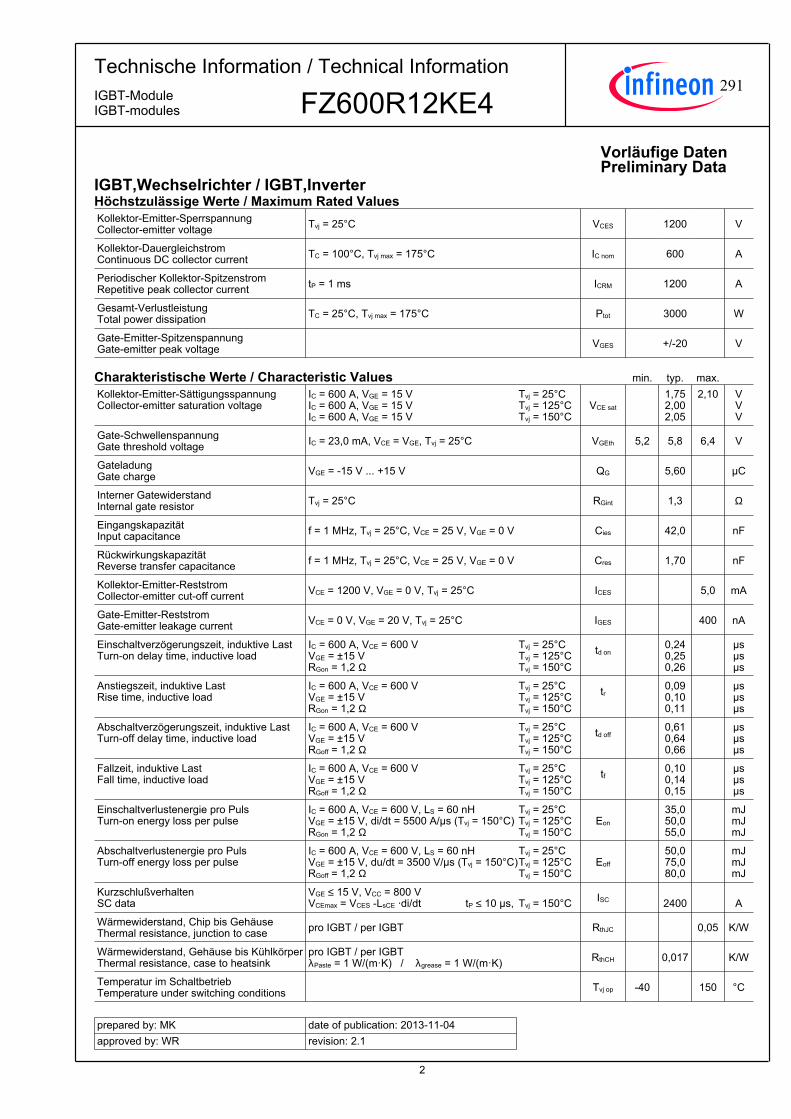
2




dateofpublication:2013-11-04revision:2.1

VorläufigeDatenPreliminaryData

IGBT,Wechselrichter/IGBT,InverterHöchstzulässigeWerte/MaximumRatedValuesKollektor-Emitter-SperrspannungCollector-emittervoltage Tvj = 25°C VCES 1200 V

Kollektor-DauergleichstromContinuousDCcollectorcurrent TC = 100°C, Tvj max = 175°C IC nom 600 A

PeriodischerKollektor-SpitzenstromRepetitivepeakcollectorcurrent tP = 1 ms ICRM 1200 A

Gesamt-VerlustleistungTotalpowerdissipation TC = 25°C, Tvj max = 175°C Ptot 3000 W

Gate-Emitter-SpitzenspannungGate-emitterpeakvoltage VGES +/-20 V

CharakteristischeWerte/CharacteristicValues min. typ. max.

Kollektor-Emitter-SättigungsspannungCollector-emittersaturationvoltage

IC = 600 A, VGE = 15 VIC = 600 A, VGE = 15 VIC = 600 A, VGE = 15 V

VCE sat

1,752,002,05

2,10

VVV

Tvj = 25°CTvj = 125°CTvj = 150°C

Gate-SchwellenspannungGatethresholdvoltage IC = 23,0 mA, VCE = VGE, Tvj = 25°C VGEth 5,2 5,8 6,4 V

GateladungGatecharge VGE = -15 V ... +15 V QG 5,60 µC

InternerGatewiderstandInternalgateresistor Tvj = 25°C RGint 1,3 Ω

EingangskapazitätInputcapacitance f = 1 MHz, Tvj = 25°C, VCE = 25 V, VGE = 0 V Cies 42,0 nF

RückwirkungskapazitätReversetransfercapacitance f = 1 MHz, Tvj = 25°C, VCE = 25 V, VGE = 0 V Cres 1,70 nF

Kollektor-Emitter-ReststromCollector-emittercut-offcurrent VCE = 1200 V, VGE = 0 V, Tvj = 25°C ICES 5,0 mA

Gate-Emitter-ReststromGate-emitterleakagecurrent VCE = 0 V, VGE = 20 V, Tvj = 25°C IGES 400 nA

Einschaltverzögerungszeit,induktiveLastTurn-ondelaytime,inductiveload

IC = 600 A, VCE = 600 VVGE = ±15 VRGon = 1,2 Ω

td on

0,240,250,26

µsµsµs

Tvj = 25°CTvj = 125°CTvj = 150°C

Anstiegszeit,induktiveLastRisetime,inductiveload

IC = 600 A, VCE = 600 VVGE = ±15 VRGon = 1,2 Ω

tr

0,090,100,11

µsµsµs

Tvj = 25°CTvj = 125°CTvj = 150°C

Abschaltverzögerungszeit,induktiveLastTurn-offdelaytime,inductiveload

IC = 600 A, VCE = 600 VVGE = ±15 VRGoff = 1,2 Ω

td off

0,610,640,66

µsµsµs

Tvj = 25°CTvj = 125°CTvj = 150°C

Fallzeit,induktiveLastFalltime,inductiveload

IC = 600 A, VCE = 600 VVGE = ±15 VRGoff = 1,2 Ω

tf

0,100,140,15

µsµsµs

Tvj = 25°CTvj = 125°CTvj = 150°C

EinschaltverlustenergieproPulsTurn-onenergylossperpulse

IC = 600 A, VCE = 600 V, LS = 60 nHVGE = ±15 V, di/dt = 5500 A/µs (Tvj = 150°C)RGon = 1,2 Ω

Eon 35,050,055,0

mJmJmJ

Tvj = 25°CTvj = 125°CTvj = 150°C

AbschaltverlustenergieproPulsTurn-offenergylossperpulse

IC = 600 A, VCE = 600 V, LS = 60 nHVGE = ±15 V, du/dt = 3500 V/µs (Tvj = 150°C)RGoff = 1,2 Ω

Eoff 50,075,080,0

mJmJmJ

Tvj = 25°CTvj = 125°CTvj = 150°C

KurzschlußverhaltenSCdata

VGE ≤ 15 V, VCC = 800 V VCEmax = VCES -LsCE ·di/dt ISC

2400 A

Tvj = 150°C

tP ≤ 10 µs,

Wärmewiderstand,ChipbisGehäuseThermalresistance,junctiontocase proIGBT/perIGBT RthJC 0,05 K/W

Wärmewiderstand,GehäusebisKühlkörperThermalresistance,casetoheatsink

proIGBT/perIGBTλPaste=1W/(m·K)/λgrease=1W/(m·K) RthCH 0,017 K/W

TemperaturimSchaltbetriebTemperatureunderswitchingconditions Tvj op -40 150 °C

291

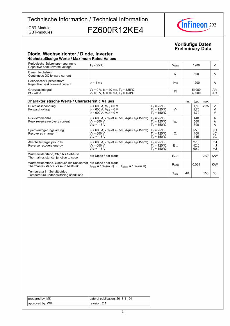
3






Diode,Wechselrichter/Diode,InverterHöchstzulässigeWerte/MaximumRatedValuesPeriodischeSpitzensperrspannungRepetitivepeakreversevoltage Tvj = 25°C VRRM 1200 V

DauergleichstromContinuousDCforwardcurrent IF 600 A

PeriodischerSpitzenstromRepetitivepeakforwardcurrent tP = 1 ms IFRM 1200 A

GrenzlastintegralI²t-value

VR = 0 V, tP = 10 ms, Tvj = 125°CVR = 0 V, tP = 10 ms, Tvj = 150°C I²t 51000

49000 A²sA²s

CharakteristischeWerte/CharacteristicValues min. typ. max.

DurchlassspannungForwardvoltage

IF = 600 A, VGE = 0 VIF = 600 A, VGE = 0 VIF = 600 A, VGE = 0 V

VF

1,801,751,70

2,35

VVV

Tvj = 25°CTvj = 125°CTvj = 150°C

RückstromspitzePeakreverserecoverycurrent

IF = 600 A, - diF/dt = 5500 A/µs (Tvj=150°C)VR = 600 VVGE = -15 V

IRM 440560590

AAA

Tvj = 25°CTvj = 125°CTvj = 150°C

SperrverzögerungsladungRecoveredcharge


Qr 55,0100115

µCµCµC

Tvj = 25°CTvj = 125°CTvj = 150°C

AbschaltenergieproPulsReverserecoveryenergy


Erec 27,052,060,0

mJmJmJ

Tvj = 25°CTvj = 125°CTvj = 150°C

Wärmewiderstand,ChipbisGehäuseThermalresistance,junctiontocase proDiode/perdiode RthJC 0,07 K/W


proDiode/perdiodeλPaste=1W/(m·K)/λgrease=1W/(m·K) RthCH 0,024 K/W

TemperaturimSchaltbetriebTemperatureunderswitchingconditions Tvj op -40 150 °C

292

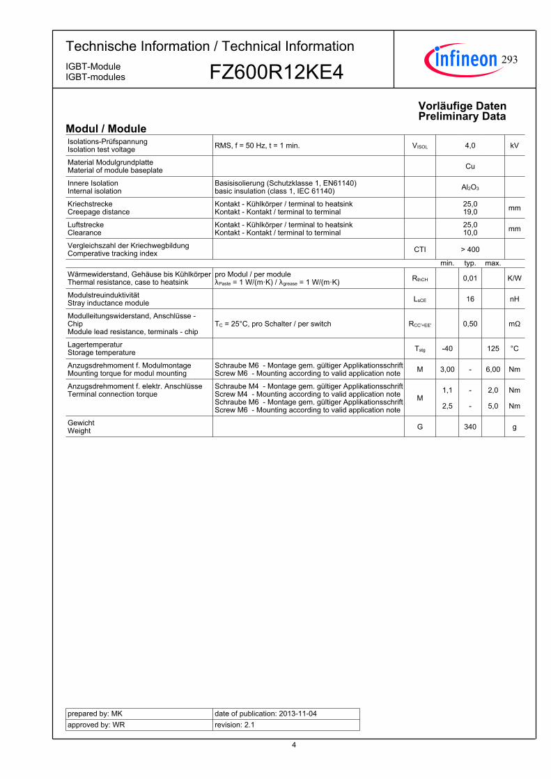
4






Modul/ModuleIsolations-PrüfspannungIsolationtestvoltage RMS, f = 50 Hz, t = 1 min. VISOL 4,0 kV

MaterialModulgrundplatteMaterialofmodulebaseplate Cu

InnereIsolationInternalisolation

Basisisolierung(Schutzklasse1,EN61140)basicinsulation(class1,IEC61140) Al2O3

KriechstreckeCreepagedistance

Kontakt-Kühlkörper/terminaltoheatsinkKontakt-Kontakt/terminaltoterminal 25,0

19,0 mm

LuftstreckeClearance

Kontakt-Kühlkörper/terminaltoheatsinkKontakt-Kontakt/terminaltoterminal 25,0

10,0 mm

VergleichszahlderKriechwegbildungComperativetrackingindex CTI > 400

min. typ. max.


proModul/permoduleλPaste=1W/(m·K)/λgrease=1W/(m·K) RthCH 0,01 K/W

ModulstreuinduktivitätStrayinductancemodule LsCE 16 nH

Modulleitungswiderstand,Anschlüsse-ChipModuleleadresistance,terminals-chip

TC=25°C,proSchalter/perswitch RCC'+EE' 0,50 mΩ

LagertemperaturStoragetemperature Tstg -40 125 °C

Anzugsdrehmomentf.ModulmontageMountingtorqueformodulmounting

SchraubeM6-Montagegem.gültigerApplikationsschriftScrewM6-Mountingaccordingtovalidapplicationnote M 3,00 - 6,00 Nm

Anzugsdrehmomentf.elektr.AnschlüsseTerminalconnectiontorque

SchraubeM4-Montagegem.gültigerApplikationsschriftScrewM4-MountingaccordingtovalidapplicationnoteSchraubeM6-Montagegem.gültigerApplikationsschriftScrewM6-Mountingaccordingtovalidapplicationnote

M1,1

2,5

-

-

2,0

5,0

Nm

Nm

GewichtWeight G 340 g

293

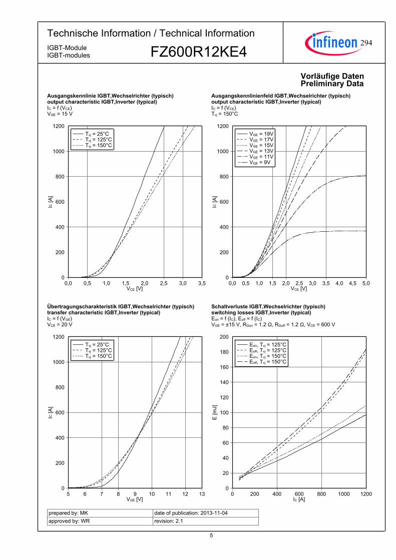
5






AusgangskennlinieIGBT,Wechselrichter(typisch)outputcharacteristicIGBT,Inverter(typical)IC=f(VCE)VGE=15V

VCE [V]

IC [A

]

0,0 0,5 1,0 1,5 2,0 2,5 3,0 3,50

200

400

600

800

1000

1200Tvj = 25°CTvj = 125°CTvj = 150°C

AusgangskennlinienfeldIGBT,Wechselrichter(typisch)outputcharacteristicIGBT,Inverter(typical)IC=f(VCE)Tvj=150°C

VCE [V]

IC [A

]

0,0 0,5 1,0 1,5 2,0 2,5 3,0 3,5 4,0 4,5 5,00

200

400

600

800

1000

1200VGE = 19VVGE = 17VVGE = 15VVGE = 13VVGE = 11VVGE = 9V

ÜbertragungscharakteristikIGBT,Wechselrichter(typisch)transfercharacteristicIGBT,Inverter(typical)IC=f(VGE)VCE=20V

VGE [V]

IC [A

]

5 6 7 8 9 10 11 12 130

200

400

600

800

1000

1200Tvj = 25°CTvj = 125°CTvj = 150°C

SchaltverlusteIGBT,Wechselrichter(typisch)switchinglossesIGBT,Inverter(typical)Eon=f(IC),Eoff=f(IC)VGE=±15V,RGon=1.2Ω,RGoff=1.2Ω,VCE=600V

IC [A]

E [m

J]

0 200 400 600 800 1000 12000

20

40

60

80

100

120

140

160

180

200Eon, Tvj = 125°CEoff, Tvj = 125°CEon, Tvj = 150°CEoff, Tvj = 150°C

294

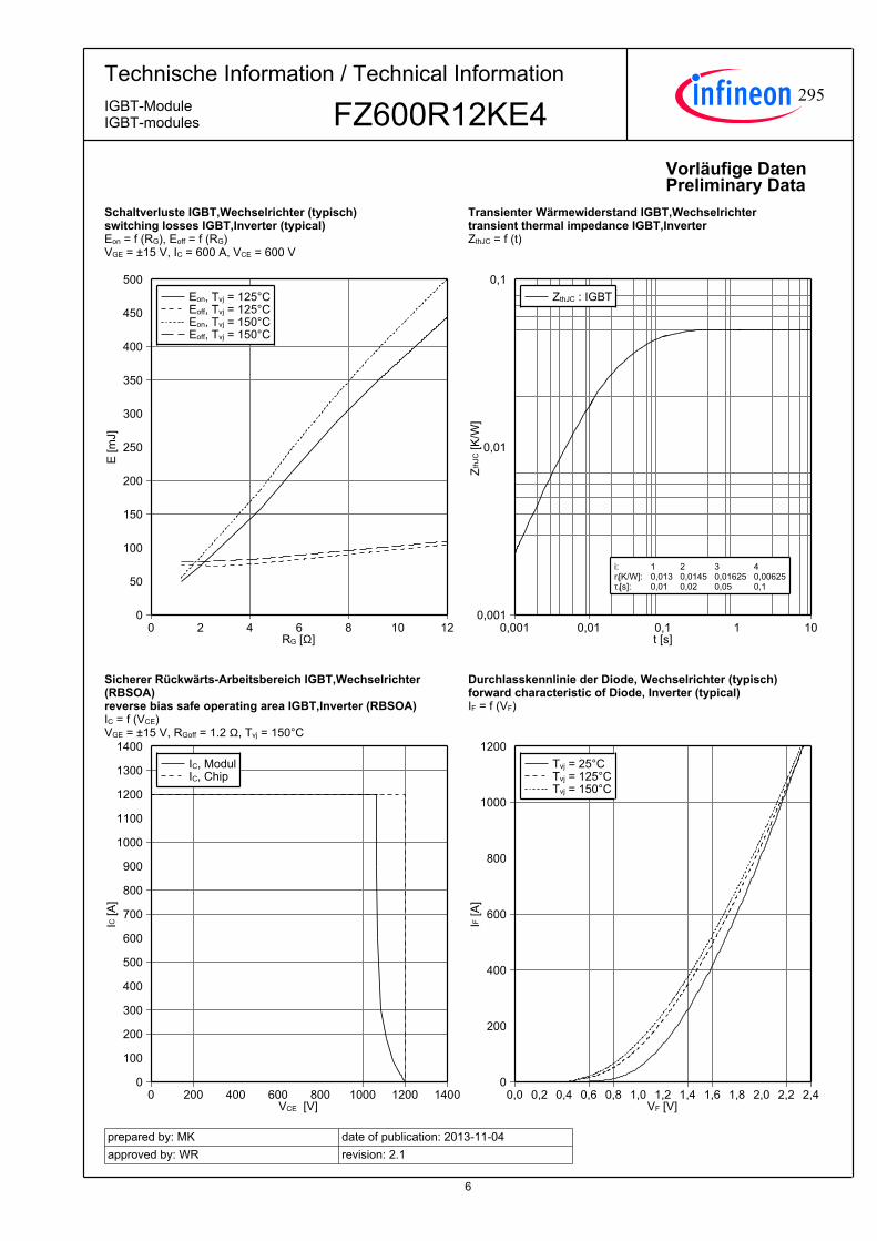
6






SchaltverlusteIGBT,Wechselrichter(typisch)switchinglossesIGBT,Inverter(typical)Eon=f(RG),Eoff=f(RG)VGE=±15V,IC=600A,VCE=600V

RG [Ω]

E [m

J]

0 2 4 6 8 10 120

50

100

150

200

250

300

350

400

450

500Eon, Tvj = 125°CEoff, Tvj = 125°CEon, Tvj = 150°CEoff, Tvj = 150°C

TransienterWärmewiderstandIGBT,WechselrichtertransientthermalimpedanceIGBT,InverterZthJC=f(t)

t [s]

Zth

JC [K

/W]

0,001 0,01 0,1 1 100,001

0,01

0,1ZthJC : IGBT

i: ri[K/W]: τi[s]:

1 0,013 0,01

2 0,0145 0,02

3 0,01625 0,05

4 0,00625 0,1

SichererRückwärts-ArbeitsbereichIGBT,Wechselrichter(RBSOA)reversebiassafeoperatingareaIGBT,Inverter(RBSOA)IC=f(VCE)VGE=±15V,RGoff=1.2Ω,Tvj=150°C

VCE [V]

IC [A

]

0 200 400 600 800 1000 1200 14000

100

200

300

400

500

600

700

800

900

1000

1100

1200

1300

1400IC, ModulIC, Chip

DurchlasskennliniederDiode,Wechselrichter(typisch)forwardcharacteristicofDiode,Inverter(typical)IF=f(VF)

VF [V]

IF [A

]

0,0 0,2 0,4 0,6 0,8 1,0 1,2 1,4 1,6 1,8 2,0 2,2 2,40

200

400

600

800

1000

1200Tvj = 25°CTvj = 125°CTvj = 150°C

295

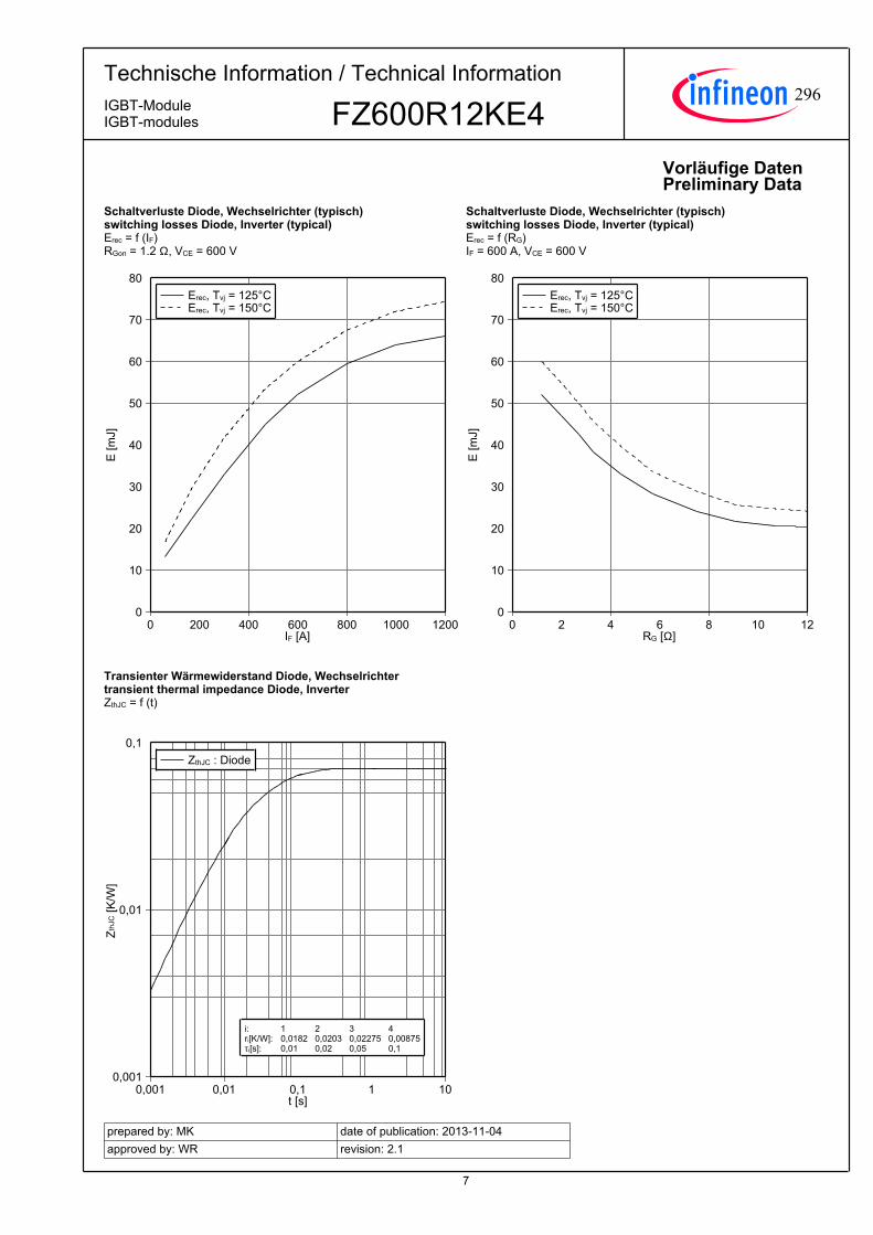
7






SchaltverlusteDiode,Wechselrichter(typisch)switchinglossesDiode,Inverter(typical)Erec=f(IF)RGon=1.2Ω,VCE=600V

IF [A]

E [m

J]

0 200 400 600 800 1000 12000

10

20

30

40

50

60

70

80Erec, Tvj = 125°CErec, Tvj = 150°C

SchaltverlusteDiode,Wechselrichter(typisch)switchinglossesDiode,Inverter(typical)Erec=f(RG)IF=600A,VCE=600V

RG [Ω]

E [m

J]

0 2 4 6 8 10 120

10

20

30

40

50

60

70

80Erec, Tvj = 125°CErec, Tvj = 150°C

TransienterWärmewiderstandDiode,WechselrichtertransientthermalimpedanceDiode,InverterZthJC=f(t)

t [s]

Zth

JC [K

/W]

0,001 0,01 0,1 1 100,001

0,01

0,1ZthJC : Diode

i: ri[K/W]: τi[s]:

1 0,0182 0,01

2 0,0203 0,02

3 0,02275 0,05

4 0,00875 0,1

296

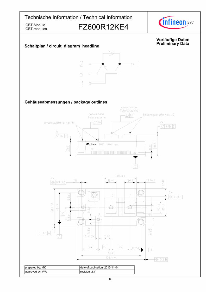
8





VorläufigeDatenPreliminaryDataSchaltplan/circuit_diagram_headline

Gehäuseabmessungen/packageoutlines

In f in e o n

297

9






NutzungsbedingungenDieindiesemProduktdatenblattenthaltenenDatensindausschließlichfürtechnischgeschultesFachpersonalbestimmt.DieBeurteilungderEignungdiesesProduktesfürIhreAnwendungsowiedieBeurteilungderVollständigkeitderbereitgestelltenProduktdatenfürdieseAnwendungobliegtIhnenbzw.IhrentechnischenAbteilungen.

IndiesemProduktdatenblattwerdendiejenigenMerkmalebeschrieben,fürdiewireineliefervertraglicheGewährleistungübernehmen.EinesolcheGewährleistungrichtetsichausschließlichnachMaßgabederimjeweiligenLiefervertragenthaltenenBestimmungen.GarantienjeglicherArtwerdenfürdasProduktunddessenEigenschaftenkeinesfallsübernommen.DieAngabenindengültigenAnwendungs-undMontagehinweisendesModulssindzubeachten.

SolltenSievonunsProduktinformationenbenötigen,dieüberdenInhaltdiesesProduktdatenblattshinausgehenundinsbesondereeinespezifischeVerwendungunddenEinsatzdiesesProduktesbetreffen,setzenSiesichbittemitdemfürSiezuständigenVertriebsbüroinVerbindung(siehewww.infineon.com,Vertrieb&Kontakt).FürInteressentenhaltenwirApplicationNotesbereit.

AufgrunddertechnischenAnforderungenkönnteunserProduktgesundheitsgefährdendeSubstanzenenthalten.BeiRückfragenzudenindiesemProduktjeweilsenthaltenenSubstanzensetzenSiesichbitteebenfallsmitdemfürSiezuständigenVertriebsbüroinVerbindung.

SolltenSiebeabsichtigen,dasProduktinAnwendungenderLuftfahrt,ingesundheits-oderlebensgefährdendenoderlebenserhaltendenAnwendungsbereicheneinzusetzen,bittenwirumMitteilung.Wirweisendaraufhin,dasswirfürdieseFälle-diegemeinsameDurchführungeinesRisiko-undQualitätsassessments;-denAbschlussvonspeziellenQualitätssicherungsvereinbarungen;-diegemeinsameEinführungvonMaßnahmenzueinerlaufendenProduktbeobachtungdringendempfehlenundgegebenenfallsdieBelieferungvonderUmsetzungsolcherMaßnahmenabhängigmachen.

Soweiterforderlich,bittenwirSie,entsprechendeHinweiseanIhreKundenzugeben.

InhaltlicheÄnderungendiesesProduktdatenblattsbleibenvorbehalten.

Terms&ConditionsofusageThedatacontainedinthisproductdatasheetisexclusivelyintendedfortechnicallytrainedstaff.Youandyourtechnicaldepartmentswillhavetoevaluatethesuitabilityoftheproductfortheintendedapplicationandthecompletenessoftheproductdatawithrespecttosuchapplication.

Thisproductdatasheetisdescribingthecharacteristicsofthisproductforwhichawarrantyisgranted.Anysuchwarrantyisgrantedexclusivelypursuantthetermsandconditionsofthesupplyagreement.Therewillbenoguaranteeofanykindfortheproductanditscharacteristics.Theinformationinthevalidapplication-andassemblynotesofthemodulemustbeconsidered.

Shouldyourequireproductinformationinexcessofthedatagiveninthisproductdatasheetorwhichconcernsthespecificapplicationofourproduct,pleasecontactthesalesoffice,whichisresponsibleforyou(seewww.infineon.com).Forthosethatarespecificallyinterestedwemayprovideapplicationnotes.

Duetotechnicalrequirementsourproductmaycontaindangeroussubstances.Forinformationonthetypesinquestionpleasecontactthesalesoffice,whichisresponsibleforyou.

ShouldyouintendtousetheProductinaviationapplications,inhealthorliveendangeringorlifesupportapplications,pleasenotify.Pleasenote,thatforanysuchapplicationsweurgentlyrecommend-toperformjointRiskandQualityAssessments;-theconclusionofQualityAgreements;-toestablishjointmeasuresofanongoingproductsurvey,andthatwemaymakedeliverydependedontherealizationofanysuchmeasures.

Ifandtotheextentnecessary,pleaseforwardequivalentnoticestoyourcustomers.

Changesofthisproductdatasheetarereserved.

298

Documents

Andersen_Kevin_MASc_2016.pdf - University of Victoria