arX

iv:0

905.

3560

v1 [

astr

o-ph

.CO

] 2

1 M

ay 2

009

Draft version September 3, 2013Preprint typeset using LATEX style emulateapj v. 08/13/06

ANISOTROPIC AGN OUTFLOWS AND ENRICHMENT OF THE INTERGALACTIC MEDIUM

Joel Germain1,2, Paramita Barai1,2, and Hugo Martel1,2

Draft version September 3, 2013

ABSTRACT

We investigate the cosmological-scale influence of outflows driven by AGNs on metal enrichmentof the intergalactic medium. AGNs are located in dense cosmological structures which tend to beanisotropic. We designed a semi-analytical model for anisotropic AGN outflows which expand awayalong the direction of least resistance. This model was implemented into a cosmological numeri-cal simulation algorithm for simulating the growth of large-scale structure in the universe. Usingthis modified algorithm, we perform a series of 9 simulations inside cosmological volumes of size(128 h−1Mpc)3, in a concordance ΛCDM universe, varying the opening angle of the outflows, thelifetimes of the AGNs, their kinetic fractions, and their level of clustering. For each simulation, wecompute the volume fraction of the IGM enriched in metals by the outflows. The resulting enrichedvolume fractions are relatively small at z & 2.5, and then grow rapidly afterward up to z = 0. We findthat AGN outflows enrich from 65% to 100% of the entire universe at the present epoch, for differentvalues of the model parameters. The enriched volume fraction depends weakly on the opening angleof the outflows. However, increasingly anisotropic outflows preferentially enrich underdense regions,a trend found more prominent at higher redshifts and decreasing at lower redshifts. The enrichedvolume fraction increases with increasing kinetic fraction and decreasing AGN lifetime and level ofclustering.Subject headings: cosmology: theory — galaxies: active — intergalactic medium — quasars: general

— methods: N-body simulations.

1. INTRODUCTION

Active galaxies are believed to be powered by ac-cretion of matter onto the central supermassive blackholes (SMBHs) (e.g., Kormendy & Richstone 1995;Ferrarese & Ford 2005), liberating enormous amountsof energy (often in the forms of ejected energeticjets/outflows), affecting their environments from pc toMpc scales. Active Galactic Nuclei (AGN) are believedto influence the formation and evolution of galaxies andlarge-scale structures over the cosmic epoch, in the formof feedback, whereby the overall properties of a galaxycan be regulated by its central BH (e.g., Silk & Rees1998; King 2003; Wyithe & Loeb 2003; Granato et al.2004; Murray et al. 2005; Begelman & Nath 2005;Pipino et al. 2009; Ciotti et al. 2009). Recent concor-dance models of galaxy formation through hierarchicalclustering in the cold dark matter cosmology invoke feed-back from AGN to explain several observations (Best2007, for a review), such as the central SMBH - hostgalaxy bulge correlations (e.g., Magorrian et al. 1998;Gebhardt et al. 2000; McLure & Dunlop 2002) and thesharp cutoff at the bright end of the galaxy luminosityfunction.

During the quasar era (1 < z < 3), the star-formationrate, the comoving density of AGN, and the merger rateof galaxies, are all observed to reach their peak values.Such a common trend points to a coevolution scenario:galaxies and AGN are argued to have evolved togetherinfluencing each other’s growth. Polletta et al. (2008)discovered two sources at z ∼ 3.5 exhibiting both pow-erful starburst and AGN activities, which is interpreted

1 Departement de physique, de genie physique et d’optique, Uni-versite Laval, Quebec, QC, Canada

2 Centre de Recherche en Astrophysique du Quebec

as a coevolution phase of star formation and AGN aspredicted by various models of galaxy formation andevolution. Observations of an AGN-starburst galaxy byCroston et al. (2008) show that AGN feedback has a sub-stantial impact on the galaxy and its surroundings. Cos-mological simulations by Di Matteo et al. (2005) indicatethat the energy released from an accreting SMBH canhalt further accretion onto the BH and drive away gas,self-regulating galaxy growth by shutting off the quasarand quenching star-formation in the galaxy, and thusreddening it rapidly.

The nature of feedback from AGN on star/galaxy for-mation can be either negative (quenching) or positive(enhancement), as shown by different studies. The exactrole played by AGNs possibly depends on one or morefactors, such as radio-loudness, jet power, lifetime/dutycycle, environmental factors like ambient gas density, etc.In galaxy clusters, AGN outflows are believed to stopthe cooling flow and heat up the intracluster medium bygiant cavities, buoyant bubbles and shock fronts (e.g.,McNamara & Nulsen 2007). At the same time, substan-tial star-formation rates are observed in the central radiogalaxies of cooling flow clusters triggered by the radiosource (McNamara 2002).

Some observations (e.g., Schawinski et al. 2007) in-dicate that AGN quench star-formation in their hostgalaxies at z < 2 turning them red and dead, in theprocess generating the observed bimodal color distribu-tion of galaxies. Hydrodynamical simulations of ma-jor mergers of equal- and unequal-mass disk and ellip-tical galaxies show that BH feedback can terminate star-formation (Springel et al. 2005; Johansson et al. 2008).Antonuccio-Delogu & Silk (2008) analyzed the differentphysical factors impacting the star-formation rate, andfound that there is suppression of star-formation in

2

galaxies from AGN jet-induced feedback. Semi-analyticmodels (Bower et al. 2006; Croton et al. 2006) show thatfeedback due to AGN can quench cooling flows andstar formation in massive halos, explaining the observeddownsizing in the stellar populations of galaxies (e.g.,Juneau et al. 2005).

Shock-induced and jet-induced star formation in radiogalaxies can explain the radio-optical alignment obser-vations. In hydrodynamic simulations including radia-tive cooling, AGN-driven shock waves compress a gascloud, causing it to break up into multiple smaller, densefragments, which survive for many dynamical timescales,turn Jeans unstable, and form stars (e.g., Mellema et al.2002; Fragile et al. 2004; van Breugel et al. 2004). Ex-panding radio jets/lobes generate shocks which propa-gate through inhomogeneous clumpy ambient gas cloudsand trigger gravitational collapse of overdense ambientgas clouds, and star formation (e.g., Begelman & Cioffi1989; De Young 1989; Rees 1989; Bicknell et al. 2000).

Studies claim to have found direct observational evi-dence for AGN feedback at z ∼ 2. Nesvadba & Lehnert(2008), using VLT data, identified kpc-sized outflows ofionized gas in z ∼ 2 − 3 radio galaxies. These bipolaroutflows have the expected signatures of being powerfulAGN-driven winds, energetic enough to terminate starformation in the massive host galaxies. At the same timethere have been few observations (e.g., Krongold et al.2007; Schlesinger et al. 2009) implying that quasar windsare unlikely to produce important evolutionary effects ontheir larger environments, which poses a challenge for thescenario of strong AGN feedback in galaxy evolution.

A fraction of AGN are radio loud, and there are claimsthat the radio-loudness depends on SMBH mass and Ed-dington ratio (e.g., Laor 2000; Rafter et al. 2009). Thelifetimes of radio sources (∼ 106 − 108 yrs) are observa-tionally inferred to be significantly shorter than the agesof their host galaxies, suggesting that the hosts cycle be-tween radio-loud and radio-quiet phases. AGN feedbackis a natural explanation: the hot ISM in a galaxy episod-ically cools to fuel the central AGN, which triggers radioactivity, and then the emanated radio jets reheat the gas(Ciotti & Ostriker 2007).

A large fraction of AGN are observed to host outflows,in a wide variety of forms (see Crenshaw et al. 2003;Begelman 2004; Everett 2007, for reviews). Radio galax-ies with collimated relativistic jets and/or huge over-pressured cocoons emitting radio synchrotron radiationconstitute ∼ 10% of all quasars (Peterson 1997). Blue-shifted broad absorption lines (BALs) in the UV and op-tical are seen in an additional ∼ 10− 15% of QSOs (e.g.,Reichard et al. 2003). Many BAL and other quasars inSDSS exhibit highly-ionized broad blue-shifted emissionlines of e.g., C IV (e.g., Richards et al. 2002). Intrin-sic absorption lines in the UV have been detected in> 50% of Seyfert I galaxies studied by Crenshaw et al.(1999). Outflows have been observed in [OIII] emis-sion lines in nearby Seyfert galaxies (e.g., Das et al.2005). Warm absorbers seen in X-rays indicate ion-ized outflows in Seyferts and QSOs (e.g., Blustin et al.2005; Krongold et al. 2007). More high-velocity highly-ionized outflows have been detected as absorption linesin X-rays (e.g., Chartas et al. 2003; Pounds et al. 2003;Dasgupta et al. 2005; O’Brien et al. 2005). The fullmechanism of AGN feedback and how it operates on dif-

ferent scales is poorly understood, both in theoreticaland observational aspects. In this paper we investigatethe impact of energetic outflows emanating from AGNon large-scale cosmological volumes.

There have been previous studies on thecosmological impact of quasar outflows atlarge scales (Furlanetto & Loeb 2001, hereafterFL01; Scannapieco & Oh 2004, hereafter SO04;Levine & Gnedin 2005, hereafter LG05). Barai (2008)used cosmological simulations to investigate the large-scale influence of radio galaxies over the Hubble time.All these studies have considered outflows expandingwith a spherical geometry. However, in realistic cosmo-logical scenarios, where the density distribution showsignificant structures in the form of filaments, pancakes,etc., outflows are expected to expand anisotropically onlarge scales. Recent observations support the pictureof anisotropic bipolar outflows on different scales.Nesvadba et al. (2008) found spectroscopic evidencefor bipolar outflows in three powerful radio galaxies atz ∼ 2 − 3, with kinetic energies equivalent to 0.2% ofthe rest-mass of the SMBH. These outflows possiblyindicate a significant phase in the evolution of the hostgalaxy. On small scales, Anathpindika & Whitworth(2008) showed that the observed outflows from youngstellar objects tend to be orthogonal to the filamentsthat contain their driving sources. Numerical simula-tions on galaxy-scales (e.g., Mac Low & Ferrara 1999;Recchi et al. 2009) show that bipolar winds and outflowsexpand preferentially along the steepest density slope,i.e., the direction perpendicular to the galaxy plane,while simulations at larger scales (Martel & Shapiro2001a,b) show that outflows emerging from cosmologicalstructures expand preferentially along the direction ofleast resistance.

The goal of our work is to study the global large-scale influence of outflows from AGN on the intergalacticmedium (IGM) in a cosmological context. We have de-signed a semi-analytical model for anisotropic outflows,which we implemented into a numerical algorithm forcosmological simulations. Using this algorithm, we sim-ulate the propagation of AGN-driven outflows into theIGM, in a ΛCDM universe. We then explore the large-scale impact of the cosmological population of AGN out-flows over the age of the universe. In this paper, wefocus on metal enrichment of the IGM, estimate the vol-ume fraction of the universe enriched by AGN outflowsas a function of redshift, and its dependence on the var-ious parameters of the model. In a forthcoming paper,we will will focus on the metal content and metallicity ofthe IGM and its observational consequences.

This paper is organized as follows. In §2 we describeour semi-analytical model for anisotropic outflows, andits implementation into a cosmological N-body simula-tion algorithm. The results are presented and discussedin §3. We present our conclusions in §4.

2. THE NUMERICAL METHOD

Our numerical method consists of three ingredients,(1) a cosmological Particle-Mesh algorithm for simulat-ing the formation and evolution of large-scale structuresin the universe, (2) a model for the masses, formationepochs, lifetimes, and spatial distributions of AGNs,and (3) a semi-analytical model for the propagation of

3

0 1 2 3 4 5 60

1•105

2•105

3•105

4•105

Num

ber

of A

GN

108 < L / LO • < 109

NAGN = 1178571

0 1 2 3 4 5 60

1•104

2•104

3•104

4•104

5•104

6•104

109 < L / LO • < 1010

NAGN = 264676

0 1 2 3 4 5 60

2.0•103

4.0•103

6.0•103

8.0•103

1.0•104

1.2•104

1.4•104

Num

ber

of A

GN

1010 < L / LO • < 1011

NAGN = 68655

0 1 2 3 4 5 60

500

1000

1500

2000

2500

3000

1011 < L / LO • < 1012

NAGN = 19372

0 1 2 3 4 5 6z

0

100

200

300

400

500

Num

ber

of A

GN

1012 < L / LO • < 1013

NAGN = 3978

0 1 2 3 4 5 6z

0

5

10

15

20

1013 < L / LO • < 1014

NAGN = 110

Fig. 1.— Redshift distribution of a total of 1 535 362 sourcesgenerated according to the QLF (§2.2) in various luminosity bins,with parameter values: TAGN = 100 Myr, and foutflow = 0.6. Thenumber of sources NAGN in each luminosity bin is indicated.

anisotropic outflows and the resulting metal-enrichmentof the IGM. We discuss these various ingredients in thefollowing subsections.

2.1. The PM Algorithm

We simulate the growth of large-scale structure ina cubic cosmological volume of comoving size Lbox =128 h−1 Mpc = 182.6 Mpc with periodic bound-ary conditions, using a Particle-Mesh (PM) algorithm(Hockney & Eastwood 1988). We use 2563 equal massparticles and a 5123 grid. This corresponds to a par-ticle mass mpart = 1.38 × 1010M⊙, and a grid spacing∆ = 0.357 Mpc. Note that this length resolution is suf-ficient for our purpose; we do not need the extra lengthresolution that a P3M algorithm would provide, and us-ing PM instead of P3M results in a major speed-up ofthe calculation. LG05 also used a PM algorithm for theirstudy of AGN outflows.

We consider a ΛCDM model with a present baryondensity parameter Ωb,0 = 0.0462, total matter (baryons+ dark matter) density parameter Ω0 = 0.279, cosmo-logical constant ΩΛ,0 = 0.721, Hubble constant H0 =70.1 km s−1Mpc−1 (h = 0.701), primordial tilt ns =0.960, and CMB temperature TCMB = 2.725, consis-tent with the results of WMAP5 combined with the datafrom baryonic acoustic oscillations and supernova stud-ies (Hinshaw et al. 2008). We generate initial conditionsat redshift z = 24, and evolve the cosmological volumeup to a final redshift z = 0.

2.2. Distribution in Redshift and Luminosity

We determine the luminosities and birth times of thecosmological AGN population by adopting the redshift-dependent luminosity distribution of AGNs from the

work of Hopkins et al. (2007) on bolometric quasar lumi-nosity function (QLF). The QLF is expressed as a stan-dard double power law,

φ(L, z) ≡dΦ

d logL=

φ⋆(L/L⋆)γ1 + (L/L⋆)γ2

, (1)

which gives the number of quasars per unit comovingvolume, per unit log luminosity interval. The values ofthe amplitude φ⋆, break luminosity L⋆, and the slopes,γ1 and γ2 evolve with redshift. We use the values givenin Table 2 of Hopkins et al. (2007), which cover the red-shift range z = 6.0 − 0.1. For a given redshift z, we getthe luminosity distribution by interpolating between twoconsecutive lines in that table. For redshifts z < 0.1, wesimply use the luminosity function at z = 0.1.

We assume that a fraction foutflow = 0.6 of AGNs pro-duce outflows (Ganguly & Brotherton 2008). The num-ber of AGNs with outflows in the simulation box of co-moving volume Vbox = L3

box, and within luminosity in-terval [L,L+ dL] at redshift z is given by

N(L, z) = foutflowVboxφ(L, z)d[logL] . (2)

We assume that AGNs have luminosities between Lmin =108L⊙ and Lmax = 1014L⊙ (Crenshaw et al. 2003). Thefiducial value for the AGN activity lifetime is taken asTAGN = 108 yr, with other values considered in §3.3.

We calculate the number and birth time of the AGNs asfollows. We divide the luminosity range L = [Lmin, Lmax]in bins of size ∆ log(L/L⊙) = 0.1. For each luminositybin, we start at redshift z = zmax = 6, and calculate thenumber of AGNs with outflows in that bin at that red-shift using equation (2). We then assign to each AGN arandom age tage between 0 (AGN just being born) andTAGN (AGN just about to die), and calculate the birthredshift zbirth = z(tmax − tage), where tmax is the cos-mic time corresponding to redshift zmax. We then moveforward in time by intervals of ∆t = 10 Myr.3 For eachnew time t, we calculate the number of AGNs with out-flows using equation (2), subtract from that number thenumber of AGNs present at earlier times that are stillalive at that time, and assign to each new AGN an agebetween 0 and ∆t (since, if that AGN was not present atthe previous time, it must have appeared during the lastinterval ∆t).

Using the QLF, we obtain the entire cosmological pop-ulation of AGNs in the simulation box starting fromzmax, namely the birth redshift (zbir), switch-off redshift(zoff) and bolometric luminosity (Lbol) of each source.Figure 1 shows the redshift distribution of the total pop-ulation of 1 535 362 sources produced using TAGN = 108

yr.

2.3. Spatial Location of AGNs

By far the AGNs have been observed (e.g.,D’Odorico et al. 2008) to be hosted in high density re-gions of the universe. In order to determine the spatiallocation of the AGNs in our simulations, we considerthe density distribution on the 512 × 512 × 512 grid,as calculated by the PM code. We filter this densityusing a gaussian filter containing a mass 1010M⊙ (e.g.,Kauffmann et al. 2003; Hickox et al. 2009), considering

3 The length of this interval does not matter as long as it issufficiently smaller than TAGN.

4

that as the minimum mass of a galaxy that might hostan AGN (for details of the filtering technique, we referthe reader to §5 of Martel 2005). We then identify all gridpoints where the value of the filtered density exceeds thevalues at the 26 neighboring grid points. These are thelocations of the density peaks.

At each timestep of the simulation, we spatially locatethe new AGNs born during that epoch (§2.2, whose zbir

values fall within the timestep interval) at the local den-sity peaks in the cosmological volume. We should haveenough peaks to assign to each new AGN an unique lo-cation, but at the same time we should locate the AGNspreferentially in high-density regions. So we adopt aredshift-dependent limiting density ρlim to select poten-tial peaks for locating the sources. We consider the peaksthat have a filtered density ρ > ρlim, and each new AGNis located at the center of one such peak, selected ran-domly but excluding peaks already containing an AGN.The number of AGN increases with time, hence we needto reduce the value of ρlim with redshift in order to se-lect a sufficient number of peaks. We use ρlim = 10ρwhen z > 3, ρlim = 7ρ when 3 ≥ z > 2, ρlim = 5ρ when2 ≥ z > 1, ρlim = 3ρ when 1 ≥ z > 0.75, and ρlim = 2ρwhen z ≤ 0.75, where ρ(z) = 3Ω0H

20 (1 + z)3/8πG is the

mean density of the universe at that redshift.Note that our method for locating AGNs differs from

the one used by LG05. In their simulations, AGNs couldbe located anywhere in the computational volume, witha probability that depended on the local density. Wehave to restrict the potential locations of AGNs to lo-cal density peaks, to be consistent with our anisotropicoutflow model (see below). This is not a severe restric-tion, because we do expect massive galaxies that hostAGNs to form at the locations of density peaks anyway.We consider alternate methods of locating the AGNs in§3.5.

2.4. Anisotropic Outflows

Pieri et al. (2007) (hereafter PMG07) have developedan anisotropic outflow model, in which outflows expand-ing into an anisotropic medium follows the path of leastresistance. The model was applied to supernovae-drivenoutflows generated by low-mass galaxies. In this paperwe apply the same model to AGN-driven outflows gen-erated by massive galaxies. The model is essentially thesame, except for some additional terms in the equationsdriving the outflow. We refer the reader to PMG07 fordetails.

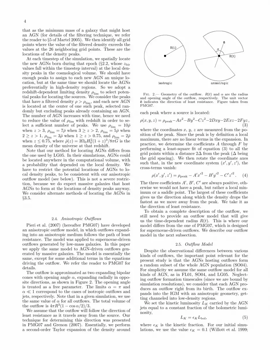
The outflow is approximated as two expanding bipolarcones with opening angle α, expanding radially in oppo-site directions, as shown in Figure 2. The opening angleis treated as a free parameter. The limits α = π andα ≪ 1 correspond to the cases of isotropic outflows andjets, respectively. Note that in a given simulation, we usethe same value of α for all outflows. The total volume ofthe outflow is 4πR3(1 − cosα/2)/3.

We assume that the outflow will follow the direction ofleast resistance as it travels away from the source. Ourtechnique for determining this direction was presentedin PMG07 and Grenon (2007). Essentially, we performa second-order Taylor expansion of the density around

Fig. 2.— Geometry of the outflow. R(t) and α are the radiusand opening angle of the outflow, respectively. The unit vectore indicates the direction of least resistance. Figure taken fromPMG07.

each peak where a source is located:

ρ(x, y, z) = ρpeak−Ax2−By2−Cz2−2Dxy−2Exz−2Fyz ,

(3)where the coordinates x, y, z are measured from the po-sition of the peak. Since the peak is by definition a localmaximum, there are no linear terms in the expansion. Inpractice, we determine the coefficients A through F byperforming a least-square fit of equation (3) to all thegrid points within a distance 2∆ from the peak (∆ beingthe grid spacing). We then rotate the coordinate axessuch that, in the new coordinate system (x′, y′, z′), thecross-terms vanish:

ρ(x′, y′, z′) = ρpeak −A′x′2−B′y′

2− C′z′

2. (4)

The three coefficients A′, B′, C′ are always positive, oth-erwise we would not have a peak, but rather a local min-imum or a saddle point. The largest of these coefficientsgives us the direction along which the density drops thefastest as we move away from the peak. We take it asthe direction of least resistance.

To obtain a complete description of the outflow, westill need to provide an outflow model that will giveus the time-dependent radius R(t). This is where ourmodel differs from the one of PMG07, which is designedfor supernovae-driven outflows. We describe our outflowmodel in the next subsection.

2.5. Outflow Model

Despite the observational differences between variouskinds of outflows, the important point relevant for thepresent study is that the AGNs hosting outflows forma random subset of the whole AGN population (SO04).For simplicity we assume the same outflow model for allkinds of AGN, as in FL01, SO04, and LG05. Neglect-ing outflow formation timescales (since we are bound bysimulation resolutions), we consider that each AGN pro-duces an outflow right from its birth. The outflow ex-pands into the IGM with an anisotropic geometry, get-ting channeled into low-density regions.

We set the kinetic luminosity LK carried by the AGNjets equal to a constant fraction of the bolometric lumi-nosity,

LK = ǫKLbol, (5)

where ǫK is the kinetic fraction. For our initial simu-lations, we use the value ǫK = 0.1 (Willott et al. 1999;

5

FL01; LG05; Chartas et al. 2007; Shankar et al. 2008),which is probably an upper limit for BAL outflows(Nath & Roychowdhury 2002), but we consider othervalues of ǫK in §3.4. SO04 used ǫK = 0.05. The totalkinetic energy transported by the jets during an AGN’sactive lifetime, EK = LKTAGN, is assumed to be con-verted to the thermal energy of the outflow.

We assume that the central black hole (of mass MBH)radiates at the Eddington limit, and provides the AGNbolometric luminosity,

Lbol =LEddington =4πGcmp

σeMBH

=1.26 × 1038erg s−1

(

MBH

M⊙

)

. (6)

Then using the ratio of central BH mass to thegalaxy bulge stellar mass, MBH/Mbulge = 0.002 (e.g.,Magorrian et al. 1998; Gebhardt et al. 2000; FL01;Marconi & Hunt 2003), and scaling it with the universalratio of the density of matter to baryons, we obtain thetotal (baryonic+dark matter) mass of the galaxy hostingthe AGN, Mgal = (Ω0/Ωb,0)Mbulge.

The model of a spherical bubble expanding as athin shell (of mass Ms) in a cosmological volume (e.g.,Tegmark et al. 1993) is used to obtain the radius, R, ofthe outflow. The rate at which IGM mass is swept up byan anisotropic outflow is given by

Ms =

0 , vp ≥ R ;

4πR2 [1 − cos (α/2)] ρx

[

R− vp

]

, vp < R ;

(7)where ρx is the density of the external gas, and vp isthe gas velocity due to infall onto the dark matter halohosting the AGN. As a simplifying approximation, weconsider that the gas density is equal to the mean baryondensity of the universe at the corresponding redshift,

ρx(z) =3H2(z)Ωb(z)

8πG=

3H20Ωb,0

8πG(1 + z)3. (8)

For the gas infall velocity, we assume vp = H(z)R, whereH(z) is the Hubble constant at redshift z. This is simplythe Hubble expansion of a cosmological volume.

After correcting for anisotropic expansion, the acceler-ation of the shell can be written as,

R=4πR2 [1 − cos (α/2)]

Ms(pT + pB − px)

−G

R2

[

Md(R) +Mgal +Ms

2

]

+ΩΛ(z)H2(z)R−Ms

Ms

[

R− vp(R)]

, (9)

where pT is the thermal pressure inside the outflow, pB isthe magnetic pressure, px is the pressure of the externalIGM, and Md(R) is the mass of matter lying inside theshell. In equation (9), the first term represents the pres-sure gradient driving the outflow outwards. The secondterm is the gravitational deceleration caused by matterexisting inside the outflow radius (attraction between theoutflow shell and the background halo + host galaxy),and the self gravity of the shell. The third term is anacceleration due to the cosmological constant. The final

term is a drag force caused by sweeping up the IGM andaccelerating it from velocity vp to R.

This formulation for the evolution of outflow radius[eq. (9)] is almost same as that of FL01, except thatwe have a factor of [1 − cos(α/2)] in the first term totake into account of the anisotropic shape of the out-flow. Tegmark et al. (1993) and PMG07 used a simi-lar equation, but they do not have the following termswhich we include for AGN outflows: the magnetic pres-sure (pB), the deceleration due to self-gravity of the shell(GMs/2R

2), and the acceleration due to the cosmologi-cal constant (ΩΛH

2R).The external gas pressure is obtained using px(z) =

ρx(z)kTx/µ, where the external temperature is fixed atTx = 104 K assuming a photoheated ambient medium,and µ = 0.611 amu is the mean molecular mass, as-suming that the medium ahead of the outflow has beenphotoionized (PMG07). The working expression for thepressure of the IGM is then

px(z) = Ωb,03H2

0kTx8πGµ

(1 + z)3. (10)

Making again the approximation that the density ofthe background through which the AGN outflows propa-gate is equal to the mean matter density of the universe,we obtain the halo mass enclosed within the shell,

Md(R, z) =4πR3

3ρ(z) =

Ω(z)H2(z)R3

2G. (11)

The thermal pressure is provided by the jet kineticpower when the AGN is active. It undergoes expansionlosses and varies at a rate

pT =Λ

2πR3 [1 − cos (α/2)]− 5pT

R

R. (12)

The first and second terms represent the increase in pres-sure caused by injection of thermal energy into the out-flow, and the drop caused by the pdV work done as theoutflow expands, respectively. The total luminosity, Λ,is the combined rate of energy deposition and dissipationwithin the outflow,

Λ = LAGN − LComp − Lne2 − Lion + Ldiss , (13)

where LAGN is the luminosity of the AGN contributingto the expansion of the outflow, LComp is the inverseCompton cooling off the CMB photons, Lne2 is the cool-ing due to two-body interactions, Lion is the cooling dueto ionization, and Ldiss is the heat dissipated from col-lisions between the expanding shell and the IGM. Weassume that the first two terms, AGN luminosity andinverse Compton cooling, dominates (following PMG07)and neglect the other terms. The Compton luminosity isgiven by

LComp =2π3

45

(

σT~

me

) (

kTγ0

~c

)4(

1 − cosα

2

)

(1+z)4pTR3 ,

(14)(PMG07) where Tγ0 is the temperature of the CMB atpresent.

Magnetic fields thread AGN jets from sub-pc to kpcscales, but their detailed characteristics are not wellknown. Following FL01, we make the simplifying as-sumption that during its activity period an AGN ejects

6

magnetic energy equal to a fixed fraction of the kineticenergy injected by the jets, EB = ǫBEK . The fractionǫB is taken as a free parameter, with a canonical valueof ǫB = 0.1. We also assume that the magnetic field (ofstrength Bm) is tangled, and exerts an isotropic pressurepB = (1/3)B2

m/8π affecting the dynamics of the out-flow. The relation between energy, pressure and volumeis EB = 3pBV . From this, we can derive the equationfor the evolution of the magnetic pressure,

pB =ǫBLAGN

4πR3 [1 − cos (α/2)]− 4pB

R

R. (15)

where the last term comes from the conservation of mag-netic flux of a magnetic field frozen into the expand-ing outflow. At early times when the AGN is active,the first term in the right-hand side dominates, andwe get pB/pT = ǫB/2. After the AGN turns off, weset LAGN = 0 (see below), and equation (15) givespB ∝ R−4. In our simulations we find that the thermalpressure always dominates over the magnetic pressure ofthe outflows.

The combination of equations (5)–(15) fully describethe evolution of the outflows. In Appendix A, we describehow these equations are solved in practice.

In our simulations we allow each AGN to evolvethrough an active life when zbir > z > zoff . Forthis time period TAGN, we use the jet kinetic luminos-ity as the AGN luminosity in equations (13) and (15),LAGN = LK = ǫKLbol.

After the central engine has stopped activity (whenz < zoff), it enters the post-AGN dormant phase. Thenwe set the AGN luminosity to zero (LAGN = 0) in equa-tions (13) and (15). The gas inside the outflow is stilloverpressured relative to the IGM, so the expansion con-tinues (e.g., Kronberg et al. 2001; Reynolds et al. 2002,PMG07, Barai 2008), but the pressure drops faster sincethere is no energy input from the AGN. The outflowkeeps expanding as long as its pressure pT + pB exceedsthe external pressure px of the IGM. When pT +pB = px,the outflow has reached pressure equilibrium. After thispoint, the outflow simply evolves passively with the Hub-ble flow.

2.6. Metal Enrichment

The material transported into the IGM by AGN out-flows, for the most part, does not originate from theAGN itself, but from the interstellar medium of the hostgalaxy. Stellar evolution in the host galaxy have enrichedthe interstellar medium with heavy elements, or metals,and these metals will be carried into the surroundingIGM by the outflows. Using our simulations, we can cal-culate the distribution and concentration of metals in theIGM. Here we focus on the distribution of metals and theenriched volume fraction, that is, the fraction of the IGMby volume that has been enriched by AGN outflows. Theconcentration of metals in the IGM will be addressed ina forthcoming paper.

To calculate the fraction of the total volume filled byoutflows, we cannot simply add up the final volumes ofthe outflows, and divide by the volume of the compu-tational box. Intergalactic gas enriched by outflows willmove with time as structures grow, and therefore regionsthat were never hit by outflows might end up containing

metals. We take this effect into account, by employinga dynamic particle enrichment scheme to quantify thecosmological enrichment history of the IGM. During theevolution of an outflow, we identify the particles thatthe outflow hits. These particles are flagged as been en-riched. This is done at every timestep for every outflowpresent in the simulation box at that time. The frac-tion of the volume of the box occupied by these enrichedparticles is then estimated, as follows.

We divide the computational volume into N3ff = 2563

cubic cells, and identify which cells contain matter thathas been enriched by outflows. Notice that we cannotsimply count the number of cells that contained parti-cles that have been flagged as enriched. This approachworks in high-density regions, but fails in low-density re-gions where the cells are smaller than the local particlespacing. We solve this problem by using a SmoothedParticle Hydrodynamics technique. A smoothing lengthh is ascribed to each particle. We calculate h iterativelyby requiring that each particle has between 60 and 100neighbors within a distance 1.7h. We then treat eachparticle as an extended sphere of radius 1.7h over whichit is considered to be spread. The cells that are coveredby one or more enriched particles are then consideredenriched. This method works well both in low- and high-density regions. The total number of filled cells, Nrich,gives the total volume of the box occupied by the en-riched particles. The fractional volume of the simulationbox enriched by AGN outflows is then Nrich/N

3ff . Notice

that this is not done during the simulation itself. Thesimulation produces dumps at various redshifts contain-ing the positions and velocities of particles, as well asthe flags which indicate which particles are enriched inmetals. The calculation of the enriched volume fractionis then performed as post-processing.

3. RESULTS AND DISCUSSION

We performed a series 9 simulations by varying someparameters of our AGN evolution model. Table 1 sum-marizes the characteristics of each run. The first columngives the letter identifying the run. In columns 2, 3, and4, we list the opening angle of the outflows, the lifetimeof the AGN’s, and the kinetic fraction, respectively. Thefifth column indicates if biasing was used when determin-ing the locations of the AGN’s. The results are presentedand discussed in the following subsections. For each runwe plot the fraction of the cosmological volume enrichedby the AGN outflows. The last column of Table 1 lists theresulting metal-enriched volume fraction at the presentepoch obtained for each run.

3.1. Evolution of a Single Outflow

Figure 3 shows the redshift evolution of a singleanisotropic outflow with opening angle α = 60, born atz ≃ 5.9. The different phases of the outflow expansionare separated by vertical lines: active phase of the AGNon the left, post-AGN phase in the middle, and passiveHubble expansion on the right. The top panel showsthe total luminosity (Λ = LAGN − LComp), the middlepanel shows the comoving radius of the outflow, and thebottom panel shows the pressures associated with theoutflow.

Soon after birth, the outflow is driven by the activeAGN, whose luminosity dominates over the Compton lu-

7

TABLE 1Parameters of the Simulation and Final Enriched Volume

Fractions

Run α () TAGN (yr) ǫK Bias in Location Nrich/N3ff(z = 0)

A 180 108 0.10 × 0.80B 120 108 0.10 × 0.82C 60 108 0.10 × 0.83D 60 107 0.10 × 1.00E 60 109 0.10 × 0.75F 60 108 0.05 × 0.79G 60 108 0.01 × 0.71H 60 108 0.10

√0.75

I 60 108 0.10√

0.65

1.0•107

1.5•107

2.0•107

2.5•107

3.0•107

Λ

(Lsu

n)

0.00.1

0.2

0.3

0.4

0.5

Rco

mov

ing

(h-1 M

pc)

Active

Post-AGN Hubble

7 6 5 4 3 2 1 0z

10-18

10-16

10-14

Pre

ssur

e (e

rg /

cm3 )

(pT + pB)

pT

pB

px

Fig. 3.— Characteristic quantities for the evolution of a singleoutflow with lifetime TAGN = 108yr, bolometric luminosity Lbol =3.3× 108L⊙, and opening angle α = 60, as a function of redshift.Upper panel: total luminosity [eq. (13), Λ = LAGN − LComp];middle panel: comoving radius of outflow (Rcomoving); lower panel:thermal pressure inside the outflow (pT , dashed), magnetic pressure(pB, dash-dot-dot-dot), total outflow pressure (pT + pB , solid),and pressure of the external IGM (px, dotted). The vertical dash-dotted lines in the lower two panels separate the different phasesof expansion of the outflow: active, post-AGN overpressured, andthe final passive Hubble evolution.

minosity, and it grows rapidly in size. At the end of theactive phase (z ≃ 5.5), the AGN turns off and the onlycontribution to the total luminosity is the energy loss byCompton drag. The interior of the outflow is still over-pressured with respect to the external IGM by a factor(pT + pB)/px ∼ 400. So it continues to expand whileits pressure falls faster (notice the change of slope in thebottom panel). Finally, when the total outflow pressurefalls to the level of the external pressure, the expansionstops. From z ≃ 1.8 the comoving radius of the outflow

7 6 5 4 3 2 1 0z

0.0

0.2

0.4

0.6

0.8

1.0

Enr

iche

d V

olum

e F

ract

ion

α = 60o

α = 120o

α = 180o

Fig. 4.— Fractional volume (Nrich/N3ff) of simulation box en-

riched by AGN outflows as a function of redshift, for various open-ing angles: α = 60 (solid), 120, (dotted), 180 (dashed). See §3.2for details.

remains constant at 0.53h−1Mpc in the passive Hubbleflow phase.

3.2. Opening Angle of Anisotropic Outflows

To study the effect of varying opening angle of the out-flows on the enriched volume fraction, we performed runsA, B, and C with opening angles α = 180, 120, and 60,respectively. Here α = 180 corresponds to the isotropicoutflow case (the geometry used by FL01, LG05, andother previous studies), and α = 60 represents the mostanisotropic outflow we consider.

Figure 4 shows the redshift evolution of the enrichedvolume fractions we obtained for different opening an-gles. The enriched volume fractions are small at z > 3,reach 0.1 at z ∼ 2, and grow rapidly afterward to 0.4 atz ∼ 1. At the present epoch, z = 0, 80% of the universe isenriched by AGN outflows. We do not find much depen-dence on the opening angle. More anisotropic outflows(smaller α) are found to enrich slightly larger volumes.Such a trend is counter-intuitive since, for a given ra-dius, an outflow with α = 180 occupies a larger volumethan one with α = 60. But according to our modelprescription in §2.5, an outflow with a smaller α growsto a larger radius than a more isotropic one, becausethe energy is concentrated into a smaller volume, result-ing in a larger pressure. Still, isotropic outflows tend tohave larger individual volumes than anisotropic ones, asPMG07 showed.

8

This effect is compensated by another effect: overlap-ping outflows. Because we locate AGNs in dense regions,they are strongly clustered, especially at low redshift. Adense region will eventually harbor many AGNs4 andtheir outflows will likely overlap. Isotropic outflows tendto overlap with one another more than anisotropic ones,for two reasons. First, for isotropic outflows the volumeoccupied by each outflow is larger, hence the probabil-ity of overlap is also larger. Second, anisotropic out-flows propagate along the direction of least resistance.As PMG07 showed, if several outflows originate from acommon structure, like a cosmological filament or pan-cake, they tend to align themselves along the directionnormal to the structure. This greatly reduces the amountof overlap, especially at small opening angle α. In oursimulations with larger α, the outflows overlap more, re-sulting in a smaller enriched volume fraction. So thecombined effect of smaller individual volumes and lessoverlap cause the more anisotropic outflows to enrich aslightly larger volume fraction of the IGM.

Figures 5 and 6 show the evolution of the large-scalestructure and the distribution of metals in a slice of co-moving thickness 2h−1Mpc, for isotropic outflows (runA), and outflows with opening angle of 60 (run C). Atz = 3.38, the metals are just starting to emerge from thedense regions that are hosting AGNs. As the simulationprogresses, new AGNs are formed, producing additionaloutflows, while the ones already present keep expandinguntil they reach pressure equilibrium with the externalIGM. By z = 1.05, a significant fraction of the volumeis enriched, but metals are still concentrated near denseregions. By z = 0, the metals have spread into the low-density regions, and only the very-low-density regions,located far from any cosmological structure, have notbeen enriched.

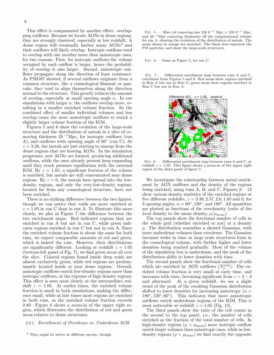
There is no striking difference between the two figures,though we can notice that voids are more enriched atz = 1.05 in run C than in run A. To illustrate this moreclearly, we plot in Figure 7 the difference between thetwo enrichment maps. Red indicates regions that areenriched in run A but not in run C, while green indi-cates regions enriched in run C but not in run A. Sincethe enriched volume fraction is about the same for bothruns, we expect comparable amounts of red and green,which is indeed the case. However, their distributionsare significantly different. Looking at redshift z = 1.05(bottom-left panel of Fig. 7), we find green areas all overthe slice. Colored regions found inside deep voids arealmost exclusively green, while red regions are predom-inantly located inside or near dense regions. Overall,anisotopic outflows enrich low-density regions more thanisotropic outflows, at the expense of high density regions.This effect is seen most clearly at the intermediate red-shift z = 1.05. At earlier times, the enriched volumefraction is small in both simulations, making the differ-ence small, while at late times most regions are enrichedin both runs, as the enriched volume fraction exceeds0.80. Figure 8 shows a zoom-in of the upper right re-gion, which illustrates the distribution of red and greenareas relative to dense structures.

3.2.1. Enrichment of Overdense vs. Underdense IGM

4 They might be active at different epochs, though.

Fig. 5.— Slice (of comoving size 128 h−1 Mpc × 128 h−1 Mpc,and 2h−1Mpc comoving thickness) off the computational volumefor run A, showing the evolution of the distribution of metals. Theareas shown in orange are enriched. The black dots represent thePM particles, and show the large-scale structures.

Fig. 6.— Same as Figure 5, for run C.

Fig. 7.— Differential enrichment map between runs A and C,calculated from Figures 5 and 6. Red areas show regions enrichedin Run A but not in Run C; green areas show regions enriched inRun C but not in Run A.

Difference A/C, z = 1.05, zoom-in

Fig. 8.— Differential enrichment map between runs A and C, atredshift z = 1.05. This figure shows a zoom-in of the upper rightregion of the third panel of figure 7.

We investigate the relationship between metal enrich-ment by AGN outflows and the density of the regionsbeing enriched, using runs A, B, and C. Figures 9 – 13show various density statistics of the enriched regions atfive different redshifts, z = 3.38, 2.57, 2.0, 1.05 and 0, for3 opening angles, α = 60, 120, and 180. All quantitiesare plotted as functions of the overdensity (ratio of thelocal density to the mean density, ρ/ρmean).

The top panels show the fractional number of cells inthe whole grid (whether enriched or not) at a densityρ. The distribution resembles a skewed Gaussian, withmore underdense volumes than overdense. The Gaussianbecomes wider in time as large scale structures form inthe cosmological volume, with further higher and lowerdensities being reached gradually. Most of the volumeof the simulation box is underdense, and the peak of thedistribution shifts to lower densities with time.

The second panels show the fractional number of cellswhich are enriched by AGN outflows (N rich

ρ ). The en-riched volume fraction is very small at early time, andincreases with time, becoming significant from z ∼ 2− 3and afterward. At a given redshift, we see a slighttrend of the peak of the resulting Gaussian distributionshifted to lower densities for increasing anisotropy (α =180, 120, 60). This indicates that more anisotropicoutflows enrich underdense regions of the IGM. This ismost noticeable at redshift z = 1.05 (Fig. 12).

The third panels show the ratio of the cell counts inthe second to the top panel, i.e., the number of cellsenriched as the fraction of the total number of cells. Inhigh-density regions (ρ > ρmean) more isotropic outflowenrich larger volumes than anisotropic ones, while in low-density regions (ρ < ρmean) we find exactly the opposite

9

0.00

0.05

0.10

0.15

Nρ

/ Nff

3

z = 3.38

0.00

0.02

0.04

0.06

0.08

Nric

h ρ / N

ff 3

60o

120o

180o

0.0

0.2

0.4

0.6

0.8

Nric

h ρ / N

ρ

-3 -2 -1 0 1 2 3log (ρ / ρmean)

1.0

1.5

2.0

Nric

h < ρ /

Nric

h < ρ

, 180

Fig. 9.— Density statistics at redshift z = 3.38 for runs A, B,and C. The quantities Nρ, Nrich

ρ , Nrich<ρ , and N3

ff= 2563 designate

the number of cells (whether enriched or not) at a given density,the number of cells enriched by AGN outflows at a given density,the number of cells enriched by AGN outflows below a given den-sity threshold, and the total number of cells in the computationalvolume, respectively. Top panel: histogram of the density distri-bution of cells. Second panel: number of cells enriched by AGNoutflows at a given density, divided by the total number of cellsin the computational volume. Third: number of cells enriched byAGN outflows at a given density, divided by the total number ofcells at that density. Bottom: number of cells enriched by AGNoutflows below a certain density threshold, divided by the corre-sponding number for the isotropic case (α = 180). The linestylesindicate the different opening angles: α = 60 (dashed), 120 (dot-ted), 180 (solid).

behavior. The effect is small, but most prominent atz = 1.05. At z = 0, dense regions are fully enriched forall values of α, while at z > 2 low-density regions arejust starting to get enriched.

The bottom panels are cumulative versions of the sec-ond panels, showing the number of enriched cells be-low a given density threshold (N rich

<ρ ), divided by the

corresponding number N rich<ρ,180 for isotropic outflows.5.

In low-density regions [log(ρ/ρmean) < 0], the ratioN rich<ρ /N

rich<ρ,180 strongly depends on the opening angle,

at all redshift but especially at early time (z ≥ 2). The

5 Note that Nrich<ρ = Nrich in the limit of large ρ. Hence, the fact

that the curves reach different asymptotes in the right hand sideof the panels simply reflects the weak dependence of the overallenriched volume fraction on opening angle.

0.00

0.05

0.10

0.15

Nρ

/ Nff

3

z = 2.57

0.00

0.02

0.04

0.06

0.08

Nric

h ρ / N

ff 3

60o

120o

180o

0.0

0.2

0.4

0.6

0.8

Nric

h ρ / N

ρ

-3 -2 -1 0 1 2 3log (ρ / ρmean)

1.0

1.5

2.0N

rich <

ρ /

Nric

h < ρ

, 180

Fig. 10.— Same as Figure 9, at redshift z = 2.57.

most anisotropic outflow (α = 60) enriches the largestunderdense volumes, and the effect is stronger at lowerdensities. The effect is most prominent at earlier epochs(z ∼ 3.5 − 2), and decreases in intensity with time, butis still visible at the present epoch. We explain thistrend as follows. At earlier times, when the AGN out-flows have just started to enrich the surrounding vol-umes, more anisotropic outflows enrich larger fractionsof the lower density IGM, since these outflows expandalong the direction of least resistance. As time goes on,large-scale structures form and grow, causing materialto accrete from low- to high-density regions. This tendsto even out the density of the enriched volumes, and astime goes on the effect of preferential enrichment of low-density regions by anisotropic outflows gets washed out.Such a trend in seen in our resulting density statistics,where the difference between the different opening anglesis very small in Figure 13 at z = 0.

3.2.2. Comparison with Pieri et al. 2007

The bottom 3 panels of Figures 9–13 are analogous tothe plots in Figure 9 of PMG07. These authors consid-ered outflows driven by SNe explosions in dwarf galax-ies, and found that the anisotropy of the outflows had amajor impact on the IGM enrichment in low-density re-gions. Outflows with opening angle α = 60 enriched thelowest-density regions of the IGM by a factor 3− 4 more

10

0.00

0.05

0.10

0.15

Nρ

/ Nff

3

z = 2

0.00

0.02

0.04

0.06

0.08

Nric

h ρ / N

ff 3

60o

120o

180o

0.0

0.2

0.4

0.6

0.8

Nric

h ρ / N

ρ

-3 -2 -1 0 1 2 3log (ρ / ρmean)

1.0

1.5

2.0

Nric

h < ρ /

Nric

h < ρ

, 180

Fig. 11.— Same as Figure 9-10, at redshift z = 2.00.

than isotropic outflows. In this study, where we consideroutflows driven by AGN in active galaxies, we find thata similar trend of increasingly anisotropic outflows to en-rich lower-density regions, but the effect depends signif-icantly on the redshift. The trend we obtained is notas dramatic as in PMG07 at the present epoch (Fig. 13),but becomes more and more prominent at earlier epochs.We find that at z = 2.57 (Fig. 10), the factor by whichoutflows with α = 60 enrich low-density regions morethan isotropic ones goes up to 1.7. At z = 3.38 (Fig. 9),the factor goes as high as 2.3.

Even though we have used the same prescription forthe anisotropic outflows as PMG07, we point out thefollowing differences between the two studies. PMG07did not perform an actual cosmological simulation.Instead, they generated an initial gaussian randomfield at high redshift, filtered that density field atvarious mass scales, and used the spherical collapsemodel to predict the collapse redshift of each halo (seeScannapieco & Broadhurst 2001 and PMG07 for details).This semi-analytical model has the advantage of simplic-ity, but does not include an accurate treatment of halomergers and accretion of matter onto halo, and further-more it underestimates the level of clustering of the halos(see, however, Pinsonneault et al. 2009). In this paper,we argue that the overlap between outflows, which re-sults from the clustering of halos, is more important for

0.00

0.05

0.10

0.15

Nρ

/ Nff

3

z = 1.05

0.00

0.02

0.04

0.06

0.08

Nric

h ρ / N

ff 3

60o

120o

180o

0.0

0.2

0.4

0.6

0.8

Nric

h ρ / N

ρ

-3 -2 -1 0 1 2 3log (ρ / ρmean)

1.0

1.5

2.0N

rich <

ρ /

Nric

h < ρ

, 180

Fig. 12.— Same as Figure 9-11, at redshift z = 1.05.

TABLE 2Runs with different active lifetimes TAGN

Run TAGN (yr) Population Size Nrich/N3ff

(z = 0)

D 107 15 279 029 1.00C 108 1 535 362 0.83E 109 162 228 0.75

isotropic outflows than anisotropic ones, and that ac-cretion of low-density, metal-enriched matter onto densestructures tends to erase the effect of anisotropy. As aconsequence, we find that the effect of anisotropy is stillimportant at high redshifts, but greatly reduced at lowredshifts.

3.3. AGN Lifetime

The simulations A, B, and C presented in the previ-ous section all assumed that AGN activity lasts TAGN =108yr. To study the effect of varying TAGN, we per-formed runs D and E, using AGN activity lifetimes ofTAGN = 107yr and 109yr, respectively. These values cor-respond to the lower limit and upper limit on TAGN usedby LG05. Simulations C, D, and E use the same openingangles, α = 60, and the same kinetic fraction, ǫK = 0.1,and differ only in the value of TAGN. We neglect any re-

11

0.00

0.05

0.10

0.15

Nρ

/ Nff

3

z = 0

0.00

0.02

0.04

0.06

0.08

Nric

h ρ / N

ff 3

60o

120o

180o

0.0

0.2

0.4

0.6

0.8

Nric

h ρ / N

ρ

-3 -2 -1 0 1 2 3log (ρ / ρmean)

1.0

1.5

2.0

Nric

h < ρ /

Nric

h < ρ

, 180

Fig. 13.— Same as Figure 9-12, at redshift z = 0.00.

7 6 5 4 3 2 1 0z

0.0

0.2

0.4

0.6

0.8

1.0

Enr

iche

d V

olum

e F

ract

ion

TAGN = 107 yr

TAGN = 108 yr

TAGN = 109 yr

Fig. 14.— Fractional volume (Nrich/N3ff) of simulation box

enriched by AGN outflows as a function of redshift, for differentAGN activity lifetimes: TAGN = 107yr (dashed), 108yr (solid),109yr (dotted). See §3.3 for details.

peated activity (which might happen because of duty cy-cle) of the same AGN after it has become inactive, as didLG05. Considering duty cycles would have a small effectin our results, because of the way we model the outflowexpansion and evolution (§2.5, our outflows continue toremain in the simulation box even after the central AGN

has died).A value of few ×108yr is considered as the typi-

cal activity lifetime of the SMBH at the centers ofactive galaxies in other studies (e.g., Yu & Lu 2008).A lifetime of 5 × 108yrs has been used in theoreti-cal modeling of radio galaxies by Blundell et al. (1999);Barai & Wiita (2007). Observations of X-ray activity inAGN (Barger et al. 2001), SDSS optical studies of ac-tive galaxies (Miller et al. 2003), and black hole demo-graphics arguments (e.g., Marconi et al. 2004) all sup-port an AGN activity lifetime of ∼ 108yr or more (also,McLure & Dunlop 2004).

Table 2 gives the parameters and results of runs C, Dand E. The first and second columns give the run nameand the value of TAGN used, respectively. Column 3 givesthe size of the AGN population, that is, the total numberof sources obtained from the QLF (§2.2) in our cosmo-logical volume over the Hubble time. The last columnlists the resulting metal-enriched volume fractions at thepresent epoch. There are ∼ 10 times more AGNs gener-ated for a decrease of TAGN by a factor of 10, since theQLF has to remain constant. This change in the num-ber of sources makes a large difference in the resultingenriched volume fractions.

The redshift evolution of the enriched volume fractionsfor different active lifetimes are plotted in Figure 14. Thelargest AGN population (TAGN = 107yr) enriches signif-icantly larger volume than the other two populations. Inthis case (run D) the fractional volume starts to becomeappreciable from z ∼ 3.5, and grows afterward, such that100% of the volume of the box is enriched by z ≃ 0.7.The other two populations, with TAGN = 108 and 109yr,enrich 0.83 and 0.75 of the volume at z = 0, respec-tively. This result, that AGNs with shorter lifetimes en-rich larger volumes than those with longer lifetimes, isopposite to what LG05 and Barai (2008) obtained. Weexplain this in the following, stressing the point that themethod we employed to enrich our cosmological volumesis quite different from what other studies have used.

We use a dynamic particle enrichment scheme (§2.6),whereby we marked particles lying inside outflow vol-umes as enriched, assign a smoothing length to each ofthem, and calculate the volume of the box being filledby these enriched particles. In other studies (LG05 andBarai 2008) the enriched volume fraction is calculated byfinding the fraction of the computational volume whichis located inside the geometrical boundaries of the out-flows. In our approach, particles that are metal-enrichedby outflows are allowed to move, and might move to re-gions not intercepted by an outflow. This increases thechance of enriching a larger fraction of the total volume.The trend heightens when the number of outflows in-crease; as more AGN are born they are placed in distinctlocations distributed throughout the box (according to§2.3), and they could potentially enrich larger volumes.This causes the enriched volume fraction to increase withincreasing population size, even though the lifetime ofeach outflow is shorter.

3.4. Kinetic Fraction

In runs F and G, we consider different values of the ki-netic fraction (the fraction of the AGN bolometric lumi-nosity which converts to the kinetic luminosity of the jets,§2.5), ǫK = 0.05 and 0.01, in addition to our standard

12

7 6 5 4 3 2 1 0z

0.0

0.2

0.4

0.6

0.8

1.0E

nric

hed

Vol

ume

Fra

ctio

n

εK = 0.1

εK = 0.05

εK = 0.01

Fig. 15.— Fractional volume (Nrich/N3ff) of simulation box

enriched by AGN outflows as a function of redshift, for differentkinetic fractions: ǫK = 0.1 (solid), 0.05 (dashed), 0.01 (dotted).See §3.4 for details.

value ǫK = 0.1 (run C). Comparing with other studies,FL01 used a value ǫK = 0.1.6 LG05 first experimentedwith a value ǫK = 0.1, and found an enriched volumefraction that was too large to agree with observations, solater they chose ǫK = 0.01 as their fiducial value. Hence,we are sampling the range of values that have been con-sidered in other studies.

The resulting enriched volume fractions are plotted inFigure 15 as a function of redshift, for the different ki-netic fractions. We find the same general trend as inruns A – E, namely that the enriched volume fraction issmall at z > 2, and then grows rapidly afterward up tothe present. At z = 0, fractions of 0.83, 0.79, and 0.71 ofthe volume are enriched by outflows with ǫK = 0.1, 0.05,and 0.01, respectively.

Using their model for the AGN outflows, LG05 foundthat the cosmological volume is completely filled (100%)by z ∼ 2 when using ǫK = 0.1 or 0.05, and withǫK = 0.01, their volume filling fraction at z = 0 is 80%.The enriched volume fractions we obtained with ǫK = 0.1and 0.05 are comparable to those obtained by LG05 withǫK = 0.01. With ǫK = 0.01, we obtained an enrichedvolume fraction ∼ 10% smaller than that of LG05. Wefind that decreasing the kinetic fraction by a factor of 10reduces the volume enriched by ≈ 12%. This is compa-rable to a corresponding ≈ 20% reduction in the volumefilling fraction found by LG05 (their Fig. 3), when ǫK isreduced by a factor of 10. It may seem surprising thatincreasing by a factor of 10 the energy driving the ex-pansion of the outflows has only a ∼ 14% effect on thefinal results. With a larger kinetic fraction, outflows arecertainly larger, but also overlap more with one another.The lowest-density regions, located far from any AGN,still manage to escape enrichment.

3.5. Bias in AGN Location

AGNs are observed to be clustered in the universe,with the clustering amplitude increasing with red-shift (Porciani et al. 2004; Croom et al. 2005; Shen et al.2007). We study the effect of bias in the distribution of

6 FL01 quote a value ǫK

= 1.0, but they expressed the quasarkinetic luminosity in terms of the B-band luminosity instead of thebolometric luminosity.

7 6 5 4 3 2 1 0z

0.0

0.2

0.4

0.6

0.8

1.0

Enr

iche

d V

olum

e F

ract

ion

Default Location

ψ = 2

Biased to Densest Peaks

Fig. 16.— Fractional volume (Nrich/N3ff) of simulation box

enriched by AGN outflows as a function of redshift, The linestylesindicate different methods of AGN location: Default run C (solid),run H with bias parameter ψ = 2, as in LG05 (dotted), run I, biasedto densest peaks (dashed). See §3.5 for details.

AGNs by considering two different methods for spatiallylocating the AGNs inside the computational volume, inaddition to our original method (§2.3) used in runs A–G.

In run H, we use a location biasing condition similarto that used by LG05, but restricted to cells containinga local density peak (this is required by our method forfinding the direction of last resistance as discussed in§2.3). We calculate the probability of each peak cell ofhosting an AGN as

P =ρψ

∑Npeak

1 (ρψ), (16)

where ρ is the filtered density (see §2.3) of the cell, Npeak

is the number of available density peaks (not containingan AGN already) inside the computational volume, andψ is the bias parameter, which is denoted by α in equa-tion (2) of LG05. The summation in the denominatorof equation (16) is over all the density peaks at the rel-evant timestep. We use a constant bias value ψ = 2,as did LG05 in their fiducial run. At each timestep, weuse a Monte Carlo rejection method to locate the AGNsrandomly, with a probability given by equation (16).

In run I, we bias the AGNs in favor of the highest-density peaks inside the cosmological volume. At eachtimestep, we find all the peak cells (§2.3), and then sortthem in descending order of their density. The new AGNs(those born in that timestep) are located in the peakcells which have the highest densities. We start withthe highest-density peak and locate one AGN (selectedrandomly from the ones just born) in it, go to the nexthighest-density peak cell and repeat the process, untilall AGNs have been assigned locations. Notice that themethods used in simulations C and I effectively corre-spond to bias parameters ψ = 0 and ψ → ∞, respec-tively.

Figure 16 shows the redshift evolution of the enrichedvolume fraction for the different location methods. Theenriched volume fraction decreases with increasing bias,at all redshifts. At z = 0, the enriched volume fractionreaches 0.83 for the case without bias (ψ = 0, run C), 0.75for the intermediate case (ψ = 2, run H), and 0.65 for themaximum bias case (ψ → ∞, run I). Such a behavior is

13

expected, as with the introduction of gradual bias AGNsare increasingly clustered in high-density regions, so theiroutflows tend to overlap. Biasing to the highest densitypeaks reduces the present enriched volume fraction by18% compared with the default case.

4. SUMMARY AND CONCLUSION

We have implemented a semi-analytical model ofanisotropic AGN outflows in cosmological N-body sim-ulations. The AGNs are placed at the location of localdensity peaks, and the outflows are allowed to expandanisotropically from those peaks, along the direction ofleast resistance, with a biconical geometry. Each AGNproduces an outflow from its birth, which at first ex-pands rapidly in the active-AGN phase for a time TAGN

until the AGN turns off, and then continues to expandslowly due to its overpressure. Finally after coming topressure equilibrium with the external IGM the outflowsimply follows the Hubble flow. The outflows carry withthem metals produced by stars in the host galaxy, andenrich the regions of the IGM that they intercept. Weused this algorithm to simulate the evolution of the large-scale structure and the propagation of outflows inside acosmological volume of size (128 h−1 Mpc)3, from initialredshift z = 24 to final redshift z = 0, in a concordanceΛCDM model. We performed a total of 9 simulations,varying the opening angle of the outflows, the active life-time of the AGNs, the kinetic fraction, and the methodused for locating the AGNs inside the cosmological vol-ume.

(1) The enriched volume fractions (fraction by volumeof the IGM enriched in metals by the outflows) are smallat z & 2.5, and then grow rapidly afterward up to z = 0.In our simulations with different parameter values, wefound that AGN outflows enrich 0.65 − 1.0 of the totalvolume of the universe by the present epoch.

(2) The enriched volume fractions do not depend sig-nificantly on the opening angle of the outflows. Moreanisotropic outflows (smaller α) are found to enrichslightly larger volumes than more isotropic ones, becausethe anisotropic ones grow bigger in radius and have lessoverlap. Increasingly anisotropic AGN outflows enrichlower-density volumes of the IGM, to an extent that de-pends on redshift. The trend is most prominent at ear-lier epochs, and not very dramatic but still visible atthe present. Outflows with opening angles α = 60 en-rich the underdense IGM more than isotropic outflowsby a factor of 2.3 at z = 3.38, and 1.7 at z = 2.57.Initially, high-density regions get enriched by outflows,since the AGNs producing these outflows are located pre-dominantly in these regions. Eventually, expanding out-

flows reach low-density regions of the IGM, and theseregions also get enriched. This effect is larger for moreanisotropic outflows, since these outflows expand alongthe directions of least resistance, reaching the low-densityregions sooner and more easily. That enriched matter,located in underdense regions at earlier epochs, gravita-tionally accretes into higher-density regions with time,as large-scale structures grow. As a result, the effectof preferential enrichment of underdense IGM by moreanisotropic outflows gets washed out with time, such thatthe difference is quite small at the present, even thoughit is quite significant at redshifts z > 1.

(3) Reducing the active lifetime TAGN of the AGNs re-sults in larger enriched volume fractions. Any reductionin TAGN must be accompanied by a corresponding in-crease in the number of AGNs, such that the observedQLF remains the same. When the number of sourcesincreases, these sources tend to be distributed more uni-formly throughout the computational volume, resultingin a more efficient enrichment. With TAGN = 107yr,100% of the volume is enriched by redshift z = 0.7.

(4) The enriched volume fractions for kinetic fractionsǫK = 0.1, 0.05 and 0.01 are 0.83, 0.79 and 0.71, respec-tively, at the present epoch. This is consistent with theresults reported by LG05. Increasing ǫK results in largeroutflows, but the main consequence is to increase thelevel of overlap, rather than the enriched volume frac-tion.

(5) We varied the prescription for locating AGNs in thecomputational volume by introducing a bias parameterwhich favors high-density peaks. This increases the levelof clustering of the AGNs, and when AGNs are more clus-tered, there is more overlap between outflows, resultingin a lower enriched volume fraction at all redshifts. Themaximum effect is an 18% decrease at z = 0 when goingfrom an unbiased distribution to a maximally biased one.

This paper focused on the metal-enriched volume frac-tion by the outflows. In a forthcoming paper, we will fo-cus on the metal abundances in the IGM resulting fromanisotropic AGN outflows, and their observational con-sequences.

We thank Philip Hopkins, Matthew Pieri, and PaulWiita for useful correspondence. The subroutine thatcalculates the direction of least resistance was writtenby Cedric Grenon. All calculations were performed atthe Laboratoire d’astrophysique numerique, UniversiteLaval. We thank the Canada Research Chair programand NSERC for support.

APPENDIX

NUMERICAL SOLUTION FOR THE OUTFLOW

In this appendix, we describe the technique used for solving the equations describing the evolution of the outflows.The presentation closely follows the one used in the appendix of PMG07.

The equations governing the evolution of the outflow are

R=4πR2[1 − cos(α/2)]

Ms(pT + pB − px) −

G

R2

[

Mgal +Ms

2

]

−Ω(z)H(z)2R

2

+ΩΛ(z)H2(z)R−Ms

Ms[R− vp(R)] , (A1)

14

Ms=

0 , vp(R) ≥ R,3Ωb(z)H

2(z)R2

2G

(

1 − cosα

2

)

[R − vp(r)] , vp(R) < R,(A2)

pT =Λ

2πR3[1 − cos(α/2)]− 5pT

R

R, (A3)

pB =ǫBLAGN

4πR3[1 − cos(α/2)]− 4pB

R

R. (A4)

with the initial conditions R = 0 at t = 0. We used equations (8) and (11) to eliminate Md and ρx in equations (A1)and (A2). Notice that since Ms ∝ 1 − cos(α/2), the dependencies of the opening angle α cancel out in the first andlast terms of equation (A1). The only remaining term in that equation that depends on α is the term −GMs/2R

2.The most important dependencies on α are found in equations (A3) and (A4). The energies (thermal and magnetic)are injected into smaller volumes, leading to larger pressures.

Many terms in equations (A1)–(A4) diverge at t = 0, making it impossible to find a numerical solution in this form(these divergences occur because we neglect the finite size of the source; in the real universe, many terms are large, butfinite, at a radius R that it small, but nonzero). To improve the behavior of the equations at early time, we performa change of variable. To find the appropriate change of variable, we take the limit t→ 0 in equations (A1)–(A4), andkeep only the leading terms. We get

R=4πR2[1 − cos(α/2)](pT + pB)

Ms−MsR

Ms, (A5)

Ms=4πR2[1 − cos(α/2)]ρx,iR , (A6)

pT =Λi

2πR3[1 − cos(α/2)]− 5pT

R

R, (A7)

pB =ǫBΛi

4πR3[1 − cos(α/2)]− 4pB

R

R. (A8)

where the subscripts i indicates initial values at t = 0. Notice that in equation (A8), we used LAGN = Λ in the limitt→ 0. We can easily show that the solutions of equations (A5)–(A8) are power laws,

R=Ct3/5 , (A9)

Ms=4πC3[1 − cos(α/2)]ρx,i

3t9/5 , (A10)

pT =7C2ρx,i

25(1 + ǫB/2)t−4/5 , (A11)

pB =7C2ρx,i

25(1 + 2/ǫB)t−4/5 , (A12)

where

C =

125Λi(1 + ǫB/2)

154πρx,i[1 − cos(α/2)]

1/5

. (A13)

Using equations (A9)–(A12), we can find the proper change of variables. We define

S=Rt2/5 , (A14)

Ns=Mst−4/5 , (A15)

qT =pT t9/5 , (A16)

qB =pBt9/5 , (A17)

U = St , (A18)

Os= Nst . (A19)

In the limit t → 0, the six functions S, Ns, qT , qB, U , and Os vary linearly with t. We now eliminate the functions R,Ms, pT and pB in our original equations (A1)–(A4) using equations (A14)–(A19) and get

U =9U

5t−

14S

25t+

4πS2(qT + qB − qx)

Nst2

(

1 − cosα

2

)

−GMgalt

11/5

S2−

ΩH2St

2

−GNst

3

2S2+ ΩΛH

2St−

[

OsNs

+4

5

] [

U

t−

2S

5t−HS

]

, (A20)

15

Ns=

−4Ns5t

, HSt+2S

5≥ U ,

3ΩbH2S2

2G

(

1 − cosα

2

)

[

U

t3−

2S

5t3−HS

t2

]

−4Ns5t

, HSt+2S

5< U ,

(A21)

qT =Λt3

2πS3[1 − cos(α/2)]−

5qTU

St+

19qT5t

, (A22)

qB =ǫBLAGN t

3

4πS3[1 − cos(α/2)]−

4qBU

St+

17qB5t

, (A23)

S=U

t, (A24)

where qx ≡ pxt9/5 in equation (A20).

These equations are completely equivalent to our original equations (A1)–(A4), but all divergences at t = 0 havebeen eliminated. These equations can therefore be integrated numerically using a standard Runge-Kutta algorithm,with the initial conditions U = S = Ns = qT = qB = 0 at t = 0. However, before doing so, it is preferable to rewritethe equations in dimensionless form. We define

τ ≡H0t , (A25)

S≡H0S

C, (A26)

U ≡H0U

C, (A27)

Ns≡GNsC3H0

, (A28)

Os≡GOsC3H0

, (A29)

qT ≡GqTC2H0

, (A30)

qB ≡GqBC2H0

, (A31)

qx≡GqxC2H0

, (A32)

fH ≡H

H0, (A33)

fΛ ≡Λ

Λi, (A34)

M≡GMgal

C3H1/50

. (A35)

Equations (A20)–(A24) reduce to their dimensionless form,

dU

dτ=

9U

5τ−

14S

25τ+

4πS2(qT + qB − qx)

Nsτ2

(

1 − cosα

2

)

−Mτ11/5

S2−

Ωf2H Sτ

2

−Nsτ

3

2S2+ ΩΛf

2H Sτ −

[

Os

Ns+

4

5

] [

U

τ−

2S

5τ− fHS

]

, (A36)

dNsdτ

=

−4Ns5τ

, fH Sτ +2S

5≥ U ,

3f2HΩbS

2

2

(

1 − cosα

2

)

[

U

τ3−

2S

5τ3−fH S

τ2

]

−4Ns5τ

, fH Sτ +2S

5< U ,

(A37)

dqTdτ

=231f2

HiΩbifΛτ3

1000πS3(1 + ǫB/2)−

5qT U

Sτ+

19qT5τ

, (A38)

dqBdτ

=231f2

HiΩbifΛτ3

1000πS3(1 + 2/ǫB)−

4qBU

Sτ+

17qB5τ

, (A39)

dS

dτ=U

τ, (A40)

16

where Os ≡ τ(dNs/dτ) in equation (A36). In the limit τ → 0, where many terms take the form 0/0, the derivatives

reduce to dS/dτ = dU/dτ = 1, dqT /dτ = 21Ωb,if2H,i/200π(1 + ǫB/2), dqB/dτ = 21Ωb,if

2H,i/200π(1 + 2/ǫB), and

dNs/dτ = Ωb,if2H,i (1 − cosα/2) /2.

The quantity fΛ appearing in equations (A38) and (A39) depends on the luminosity LComp, which is given byequation (14). We eliminate PT and R in equation (14), using equations (A14), (A16), (A25), (A26), and (A30), theneliminate C using equation (A13). We get

LComp

Li=

200π3

2079

σT ~

meH0Ωb,if2H,i

(

kTγ0

~c

)4

(1 + z)4 qT S

3

τ3. (A41)

17

REFERENCES

Anathpindika, S., & Whitworth, A. P. 2008, A&A, 487, 605Antonuccio-Delogu, V., & Silk, J. 2008, MNRAS, 389, 1750Barai, P. 2008, ApJ, 682, L17Barai, P., & Wiita, P. J. 2007, ApJ, 658, 217Barger, A. J. et al. 2001, AJ, 122, 2177Begelman, M. C., & Cioffi, D. F. 1989, ApJ, 345, L21Begelman, M. C. 2004, in Coevolution of black Holes and Galaxies,

Carnegie Observatories Astrophysics Series, ed. L. C. Ho, p. 374Begelman, M. C., & Nath, B. B. 2005, MNRAS, 361, 1387Best, P. N. 2007, NewAR, 51, 168Bicknell, G. V. et al. 2000, ApJ, 540, 678Blundell, K. M., Rawlings, S., & Willott, C. J. 1999, AJ, 117, 677Blustin, A. J., Page, M. J., Fuerst, S. V., Branduardi-Raymont, G.

& Ashton, C. E. 2005, A&A, 431, 111Bower, R. G. et al. 2006, MNRAS, 370, 645Chartas, G., Brandt, W. N., & Gallagher, S. C. 2003, ApJ, 595, 85Chartas, G., Brandt, W. N., Gallagher, S. C., & Proga, D. 2007,

AJ, 133, 1849Ciotti, L., & Ostriker, J. P. 2007, ApJ, 665, 1038Ciotti, L., Ostriker, J. P. & Proga, D. 2009, ApJ, submitted (arXiv:

0901.1089)Crenshaw, D. M., Kraemer, S. B., Boggess, A., Maran, S. P.,

Mushotzky, R. F., & Wu, C.-C. 1999, ApJ, 516, 750Crenshaw, D. M., Kraemer, S. B., & George, I. M. 2003, ARA&A,

41, 117Croom, S. M. et al. 2005, MNRAS, 356, 415Croston, J. H., Hardcastle, M. J., Kharb, P., Kraft, R. P., & Hota,

A. 2008, ApJ, 688, 190Croton, D. J. et al. 2006, MNRAS, 365, 11Das, V. et al. 2005, AJ, 130, 945Dasgupta, S., Rao, A. R., Dewangan, G. C., & Agrawal, V. K.

2005, ApJ, 618, L87De Young, D. S. 1989, ApJ, 342, L59Di Matteo, T., Springel, V., & Hernquist, L. 2005, Nature, 433,

604D’Odorico, V., Bruscoli, M., Saitta, F., Fontanot, F., Viel, M.,

Cristiani, S. & Monaco, P. 2008, MNRAS, 389, 1727Everett, J. E. 2007, Ap&SS, 311, 269Ferrarese, L., & Ford, H. 2005, SSRv, 116, 523Fragile, P. C., Murray, S. D., Anninos, P., & van Breugel, W. 2004,

ApJ, 604, 74Furlanetto, S. R., & Loeb, A. 2001, ApJ, 556, 619 (FL01)Ganguly, R., & Brotherton, M. S. 2008, ApJ, 672, 102Gebhardt, K. et al. 2000, ApJ, 539, L13Granato, G. L., De Zotti, G., Silva, L., Bressan, A., & Danese, L.

2004, ApJ, 600, 580Grenon, C., Master’s Thesis (Universite Laval, 2007)Hickox, R. C. et al. 2009, ApJ, in press (arXiv:0901.4121)Hinshaw, G. et al. 2008, ApJS, 180, 225Hockney, R. W., & Eastwood, J. W. 1988, Computer Simulation

Using Particles (New York: Adam Hilger).Hopkins, P. F., Richards, G. T., & Hernquist, L. 2007, ApJ, 654,

731Johansson, P. H., Naab, T. & Burkert, A. 2008, conference

proceedings, arXiv:0809.3399Juneau, S. et al. 2005, ApJ, 619, L135Kauffmann, G. et al. 2003, MNRAS, 346, 1055King, A. 2003, ApJ, 596, L27Kormendy, J., & Richstone, D. 1995, ARA&A, 33, 581Kronberg, P. P., Dufton, Q. W., Li, H., & Colgate, S. A. 2001, ApJ,

560, 178Krongold, Y., Nicastro, F., Elvis, M., Brickhouse, N., Binette, L.,

Mathur, S., & Jimenez-Bailon, E. 2007, ApJ, 659, 1022Laor, A. 2000, ApJ, 543, L111Levine, R., & Gnedin, N. Y. 2005, ApJ, 632, 727 (LG05)Mac Low, M.-M., & Ferrara, A. 1999, ApJ, 513, 142

Magorrian, J. et al. 1998, AJ, 115, 2285Marconi, A., & Hunt, L. K. 2003, ApJ, 589, L21Marconi, A., Risaliti, G., Gilli, R., Hunt, L. K., Maiolino, R., &

Salvati, M. 2004, MNRAS, 351, 169Martel, H. 2005, Technical Report UL-CRC/CTN-RT003

(astro-ph/0506540)Martel, H., & Shapiro, P. R. 2001a, RevMexAA, 10, 101

Martel, H., & Shapiro, P. R. 2001b, in Relativistic Astrophysics,AIP Conference Proceedings 586, eds. J. C. Wheeler & H.Martel, p. 265

McLure, R. J., & Dunlop, J. S. 2002, MNRAS, 331, 795McLure, R. J., & Dunlop, J. S. 2004, MNRAS, 352, 1390McNamara, B. R. 2002, NewAR, 46, 141McNamara, B. R., & Nulsen, P. E. J. 2007, ARA&A, 45, 117Mellema, G., Kurk, J. D., & Rottgering, H. J. A. 2002, A&A, 395,

L13Miller, C. J., Nichol, R. C., Gomez, P. L., Hopkins, A. M., &

Bernardi, M. 2003, ApJ, 597, 142Murray, N., Quataert, E., & Thompson, T. A. 2005, ApJ, 618, 569Nath, B. B., & Roychowdhury, S. 2002, MNRAS, 333, 145Nesvadba, N. P. H., Lehnert, M. D., De Breuck, C., Gilbert, A. M.,

& van Breugel, W. 2008, A&A, 491, 407Nesvadba, N. P. H. & Lehnert, M. D. 2008, SF2A-2008, Proceedings

of the annual meeting of the French Society of Astronomy andAstrophysics, eds. C. Charbonnel, F. Combes & R. Samadi, p 377

O’Brien, P. T., Reeves, J. N., Simpson, C., & Ward, M. J. 2005,MNRAS, 360, L25

Peterson, B. M. 1997, An introduction to active galactic nuclei,Cambridge (New York), Cambridge University Press

Pieri, M. M., Martel, H., & Grenon, C. 2007, ApJ, 658, 36 (PMG07)Pinsonneault, S., Pieri, M. M., & Martel, H. 2009, in preparationPipino, A., Silk, J., & Matteucci, F. 2009, MNRAS, 392, 475Polletta, M. et al. 2008, A&A, 492, 81Porciani, C., Magliocchetti, M., & Norberg, P. 2004, MNRAS, 355,

1010Pounds, K. A., King, A. R., Page, K. L., & O’Brien, P. T. 2003,

MNRAS, 346, 1025Rafter, S. E., Crenshaw, D. M., & Wiita, P. J. 2009, AJ, 137, 42Recchi, S., Hensler, G. & Anelli, D. 2009, in Star-forming Dwarf

Galaxies: Ariane’s Thread in the Cosmic Labyrinth, in press(arXiv: 0901.1976)

Rees, M. J. 1989, MNRAS, 239, 1PReichard, T. A. et al. 2003, AJ, 126, 2594Reynolds, C. S., Heinz, S., & Begelman, M. C. 2002, MNRAS, 332,

271Richards, G. T. et al. 2002, AJ, 124, 1Scannapieco, E., & Broadhurst, T. 2001, ApJ, 549, 28Scannapieco, E., & Oh, S. P. 2004, ApJ, 608, 62 (SO04)Schawinski, K. et al. 2007, MNRAS, 382, 1415Schlesinger, K., Pogge, R. W., Martini, P., Shields, J. C. & Fields,

D. 2009, preprint (arXiv: 0902.0004)Shankar, F., Cavaliere, A., Cirasuolo, M., & Maraschi, L. 2008,

ApJ, 676, 131Shen, Y. et al. 2007, AJ, 133, 2222Silk, J., & Rees, M. J. 1998, A&A, 331, L1Springel, V., Di Matteo, T., & Hernquist, L. 2005, ApJ, 620, L79Tegmark, M., Silk, J., & Evrard, A. 1993, ApJ, 417, 54van Breugel, W., Fragile, C., Anninos, P., & Murray, S. 2004, IAUS,

217, 472Willott, C. J., Rawlings, S., Blundell, K. M., & Lacy, M. 1999,

MNRAS, 309, 1017Wyithe, J. S. B., & Loeb, A. 2003, ApJ, 595, 614Yu, Q., & Lu, Y. 2008, ApJ, 689, 732