Antarctic icebergs distributions, 2002–2010

Jean Tournadre,1 Fanny Girard-Ardhuin,1 and Benoit Legrésy2

Received 8 July 2011; revised 15 March 2012; accepted 16 March 2012; published 1 May 2012.

[1] Interest for icebergs and their possible impact on southern ocean circulation andbiology has increased during the recent years. While large tabular icebergs areroutinely tracked and monitored using scatterometer data, the distribution of smallericebergs (less than some km) is still largely unknown as they are difficult to detectoperationally using conventional satellite data. In a recent study, Tournadre et al.(2008) showed that small icebergs can be detected, at least in open water, using highresolution (20 Hz) altimeter waveforms. In the present paper, we present animprovement of their method that allows, assuming a constant iceberg freeboardelevation and constant ice backscatter coefficient, to estimate the top-down icebergsurface area and therefore the distribution of the volume of ice on a monthly basis.The complete Jason-1 reprocessed (version C) archive covering the 2002–2010 periodhas been processed using this method. The small iceberg data base for the southernocean gives an unprecedented description of the small iceberg (100 m–2800 m)distribution at unprecedented time and space resolutions. The iceberg size, which followsa lognormal distribution with an overall mean length of 630 m, has a strong seasonalcycle reflecting the melting of icebergs during the austral summer estimated at 1.5 m/day.The total volume of ice in the southern ocean has an annual mean value of about 400 Gt,i.e., about 35% of the mean yearly volume of large tabular icebergs estimated from theNational Ice Center database of 1979–2003 iceberg tracks and a model of icebergthermodynamics. They can thus play a significant role in the injection of meltwater in theocean. The distribution of ice volume which has strong seasonal cycle presents a veryhigh spatial and temporal variability which is much contrasted in the three ocean basins(South Atlantic, Indian and Pacific oceans). The analysis of the relationship betweensmall and large (>5 km) icebergs shows that a majority of small icebergs are directlyassociated with the large ones but that there are vast regions, such as the eastern branch ofthe Wedell Gyre, where the transport of ice is made only through the smaller ones.

Citation: Tournadre, J., F. Girard-Ardhuin, and B. Legrésy (2012), Antarctic icebergs distributions, 2002–2010, J. Geophys.Res., 117, C05004, doi:10.1029/2011JC007441.

1. Introduction

[2] Interest in icebergs has been growing in recent years(see for example the recent review by Smith [2011] as theymay account for a significant part of the freshwater flux in thesouthern ocean [Silva et al., 2006;Martin and Adcroft, 2010;Gladstone et al., 2001; Jongma et al., 2009], and becausethey have been shown to transport nutriments (in particularlabile iron) that could have a significant impact on oceanprimary productivity [Schodlok et al., 2006; Raiswell et al.,2008; Lancelot et al., 2009; Schwarz and Schodlok, 2009].Contrary to large tabular icebergs that are routinely tracked

and monitored using scatterometer data [Long et al., 2002],the distribution of smaller icebergs, i.e., less than 2–3 km inlength, in the southern ocean is known mainly from ship-based observations with a limited temporal and spatial cov-erage [Jacka and Giles, 2007; Wadhams, 1988; Romanovet al., 2008]. Indeed, they are difficult to detect operation-ally using satellite borne sensors. Visible and infrared sensorsare often blinded by clouds while low resolution microwavesensors, such as radiometers, cannot detect such small fea-tures. Microwave scatterometer have been used regionallyand with limitations to establish statistics on icebergs incoastal areas [Young et al., 1998]. Synthetic Aperture Radars,although their detecting capabilities have been demonstrated[Gladstone and Bigg, 2002; Silva and Bigg, 2005] they haveyet to be used on an operational basis to produce icebergdistribution or climatology, mainly due to the large amountof data to be processed.[3] In a recent study, Tournadre et al. [2008] demon-

strated that small icebergs, at least in open water, have asignificant signature in the noise part of high resolution (HR)

1Laboratoire d’Océanographie Spatiale, Ifremer, Plouzane, France.2LEGOS, CNRS-CNES-IRD-UPS, Toulouse, France.

Corresponding Author: J. Tournadre, IFREMER, Laboratoired’Océanographie Spatiale, BP70, F-29280 Plouzané, France.(jean.tournadre@ifremer.fr)

Copyright 2012 by the American Geophysical Union.0148-0227/12/2011JC007441

JOURNAL OF GEOPHYSICAL RESEARCH, VOL. 117, C05004, doi:10.1029/2011JC007441, 2012

C05004 1 of 15

altimeter waveforms and that the analysis of Jason altimeterHR waveforms over the southern ocean enables to determinethe small iceberg distribution on a monthly basis. However,their study covers only one year of Jason-1 data. The recentavailability of the reprocessed Jason 1 archive, which nowcovers more than 9 years, allows a first estimate of smalliceberg climatology. The distribution of small icebergs iscertainly of importance per se for climate studies, but for theanalysis of the impact of icebergs on biomass, for the esti-mate of fresh water flux in the ocean or for ocean circulation,the volume of ice is certainly a more pertinent parameter.The detection method proposed by Tournadre et al. [2008],which provides only the location of icebergs and an estimateof the minimum iceberg freeboard height, is here improvedto provide an estimate, under the assumption of a constantice backscatter and on a constant iceberg freeboard eleva-tion, of the top-down iceberg surface area and volume thatare then used to compute the monthly distribution of thevolume of ice (see section 2). In section 3, the analysis of thespatiotemporal variability of the distribution of iceberg sizeand of the volume of ice from 2002 to 2010 is presented;their relation with large icebergs is then investigated insection 4 while the final section gives an estimate of thequantity of fresh water available from small icebergs in thesouthern ocean.

2. The Iceberg Data Set

2.1. Analysis of Jason-1 Archives (2002–2010)

[4] The CNES/NASA Jason-1 mission, launched onDecember 7th, 2001, was designed to ensure the continuityof the observation and monitoring of the ocean provided byTopex/Poseidon and it has basically the same characteristics.Its main instrument is the Poseidon-2 altimeter, which wasderived from the experimental Poseidon-1 altimeter onboard Topex/Poseidon. Poseidon-2 is a dual frequency radaroperating at 13.6 GHz (Ku band) and 5.3 GHz (C band).Depending on sea state, the altimeter footprint varies from 5to 10 km radius. The satellite samples the ocean surfacebetween 66�S and 66�N at a 0.05-s interval for each of the254 passes that make up a 9.9156-day repeat cycle. Adetailed description of the Poseidon-2 altimeter is given inMénard and Fu [2001]. The main Jason-1 altimeter char-acteristics are the following: altitude 1324 km, inclination66�, waveform frequency 20 Hz, pulse repetition frequency1800 Hz, number of waveforms on average 90 per 0.05 s,telemetry bin width 3.125 ns, nominal track point 32.5.[5] The CLS/AVISO Sensor Geophysical Data Records

(SGDR version C) data set that contains the high resolution(20 Hz) altimeter waveforms given in telemetry bins (gate)of width 3.125 ns (length of the pulse) is used in thepresent study. This data set is available upon request at theAVISO Center (http://www.aviso.oceanobs.com). These20 Hz waveforms are themselves an average of 90 individualechoes to reduce the speckle noise. The distance betweentwo consecutive HR waveforms is 290 m.[6] Nine years of Jason-1 Ku and C-band 20 Hz wave-

forms from January 25th, 2002 to December 31st, 2010(cycles 2 to 331) have been processed using the detectionmethod presented by Tournadre et al. [2008] to produce aniceberg database for the southern ocean. A detaileddescription of the method is given in Appendix A. Basically

an altimeter is a nadir looking radar that emits short pulsesthat are backscattered by the sea surface. The altimetermeasures the backscattered power as a function of time toconstruct the echo waveform from which the geophysicalparameters are estimated. Targets emerging from the seasurface, such as icebergs or ships, can produce a detectableecho before the sea surface, i.e., in the noise part of thealtimeter waveforms [Tournadre, 2007]. This signature isdetectable, if the backscattered power is high enough tocome out of the thermal noise of the sensor and if the time ofthe echo is within the measurement window of the system.This signature has a parabolic shape in the waveform spacethat depends only on the characteristics of the satellite orbitand can be easily detected using convolution analysis. Thedetection algorithm proposed by Tournadre et al. [2008]gives the location of the icebergs as well as the time of theecho tech and the power backscattered by the iceberg, siceb.[7] More than fifty-two thousand iceberg signatures were

detected and analyzed in open water between 66�S and 45�Sfor the 2002–2010 period. Due to the 66� inclination of theJason-1 orbit, the satellite inter-track distance decreases withlatitude up to 66�S (from 315 km at the equator to 132 km at65�S). As the density of altimeter data available on a regulargrid thus increases poleward with latitude, the number ofdetected icebergs will be biased toward larger values at ahigher latitude. To obtain a spatially consistent distribution itis thus necessary to consider the probability of the presenceof icebergs rather than the number of detections. Thisprobability P of the presence of icebergs is simply the ratioof the number N of icebergs detected within a grid cell by thenumber Ns of valid Jason-1 samples within the same grid cell

P i; jð Þ ¼ N i; jð Þ=Ns i; jð Þ: ð1Þ

2.2. Estimate of the Icebergs Area and Ice Volume

2.2.1. Iceberg Area[8] The method of detection provides the time of the echo

(i.e., the range) as well as the mean backscatter. The rangedepends on the distance d from nadir of the iceberg centerand on the freeboard elevation h of the iceberg. In theirstudy, Tournadre et al. [2008] estimated the minimumfreeboard of an iceberg, i.e., the freeboard that an icebergwould have if located at the satellite nadir (d = 0). The meanbackscatter depends not only on the area, A, and on thedistance from nadir but also on the backscattering coefficientof the iceberg surface, s0

ice, which is conditioned by the icecharacteristics, the shape and roughness of the iceberg sur-face, and the presence on the iceberg surface of snow orwater. The two parameters, tech and siceb, are thus functionof four main unknowns, d, A, h and s0

ice. The iceberg areacan be estimated if assumptions are made on the values oftwo of the remaining unknowns (d, h s0

ice).[9] First, we assume that the backscatter coefficient of the

iceberg surface is the same for all icebergs. This assumptionis certainly quite a crude approximation and has to be veri-fied at least at a first order. Let us first assume that the largestmeasured backscatter corresponds to the largest icebergs,i.e., icebergs that almost completely fill the altimeter foot-print and that the size of the largest detectable icebergsvaries only weakly with time, latitude and longitude. Theanalysis of the maximum of siceb as a function of latitude,longitude and time can then be used to validate at first order

TOURNADRE ET AL.: ICEBERG DISTRIBUTION C05004C05004

2 of 15

the hypothesis of constant surface backscatter of iceberg.The mean value and standard deviation of 2% of the highestvalues, robust estimators [Horn, 1990] of the sample maxi-mum, are thus used to analyze the maximum siceb and itsvariability. Figure 1 presents the variation of the maximumsiceb as a function of latitude and year as well as the stan-dard deviation and the number of samples in each latitude-year class. The latitude bins were chosen to equalize as faras possible the number of samples per bins (see Figure 1c).The maximum and standard deviation (std) computed forthe nine year period are also presented in the figure. Binscontaining less than 10 samples were not considered. Themaximum value decreases slightly with latitude between65 and 50�S (by �0.3 to �0.8 dB depending on the year)and this meridional variation reflects, at least partly, themean decrease in iceberg area with latitude. The inter-annual variability in each latitude bin ranges from 0.5 dBto 0.81 dB while the std remains stable around 0.8 dB.Very similar results were found on the zonal variability(figure not presented here). The maximum siceb appearsthus quite stable, especially when considering the vari-ability of iceberg distribution as well as the noise level onaltimeter backscatter measurement (about 0.5 dB). Thehypothesis of a constant iceberg surface backscatter coef-ficient can be thus be considered as valid as in a firstorder approximation.[10] To our knowledge, no studies have been published on

the Ku-band quasi-specular backscatter of small icebergs.However, studies have been published on the analysis ofEnvisat Ku-band backscatter over ice caps [Legrésy et al.,2005; Tran et al., 2008, 2009]. Over flat surfaces such ascentral Greenland or the Droning Maud Land, the Ku-bandsurface backscatter is in the order of 15–16 dB. Using thisvalue for iceberg surface backscatter and +2.9 dB inter-

calibration correction between the Envisat and Jason-1 Kuband backscatter coefficient estimated by Faugère et al.[2006], the iceberg surface backscatter s1 is set at 19 dB.[11] Secondly, it is necessary to fix either a mean distance

from nadir of the icebergs or a mean iceberg freeboard ele-vation. As the distance from nadir is a purely random vari-able with uniform probability and as it has a stronger impacton backscatter than the freeboard elevation [Tournadreet al., 2008], we choose to assume a constant freeboardelevation. Following Gladstone et al. [2001] the freeboardelevation for icebergs larger than 200 m, is set at 28 mcorresponding to a mean iceberg thickness of 250 m (usingDowdeswell and Bamber’s [2007] formula for summer).This freeboard corresponds to the average freeboard over theiceberg and is lower than the values proposed by Romanovet al. [2011] for icebergs of different shapes but corre-sponds to an average freeboard over the iceberg and not theiceberg maximum visible vertical dimension as obtainedfrom ship observations.[12] Using the fixed freeboard and surface backscatter

assumptions, the analytical model of waveforms presentedby Tournadre et al. [2008] (see equation (A3)) is used tocompute the signature of icebergs as a function of distancefrom nadir, (0 to 12 km), and area (0.01 to 9 km2). Forsimplicity, icebergs are assumed square. The time of theecho tech = f(d, A) and the mean backscatter siceb = g(d, A)are estimated from the modeled waveforms and are thenused to compute the inverse model A = l(tech, siceb) andd = m(tech, siceb) presented in Figure 2. The results of thewaveform modeling shows a saturation of siceb around15 dB for icebergs larger than �8 km2. The differencebetween the maximum backscatter and the surface back-scatter results from the fact that 28 m freeboard icebergs canonly be detected off nadir (d > 5 km) which introduces an

Figure 1. (a) Mean value and (b) standard deviation of the 2% of the highest siceb, as a function of yearand latitude, and (c) number of samples per bins.

TOURNADRE ET AL.: ICEBERG DISTRIBUTION C05004C05004

3 of 15

attenuation of the signal due to the antenna beam patternand the surface sampling geometry of the altimeter (seeAppendix A). This maximum value of 15 dB is close to theobserved mean value of the maximum backscatter and cor-roborates the choice of s0

ice.[13] The inverse model is applied to the range and back-

scatter of the detected icebergs to estimate the area and dis-tance from nadir. Figure 3 presents the rescaled frequencyhistogram, (i.e., an estimator of the probability densityfunction) of the areas. As suggested by Wadhams [1988] foriceberg length, the area distribution follows quite well a two-parameter lognormal distribution fX of the form

fX x;m;sð Þ ¼ 1

xsffiffiffiffiffiffi2p

p e�ln x�mð Þ22s2 ; x > 0; ð2Þ

where m and s are the location and scale parametersrespectively. The Maximum Likelihood Estimations (MLE)(see for example Wilks [2006] for the estimation method) ofm and s2 at a 99% confidence level are respectively 12.26

and 1.56. The mean of the distribution, defined by emþs22 , is

7.33105 m = 0.733 km2. As most past studies published on

the size of iceberg were based on the analysis of ship bornedata and they analyzed the apparent diameter [Wadhams,1988] or the maximum horizontal dimension at the water-line [Romanov et al., 2011], the histogram of the iceberglength (i.e.,

ffiffiffiA

p) is also computed and a lognormal distri-

bution fitted to the data. The MLE of m and s2 at a 99%confidence level for the iceberg length are respectively 6.14and 0.61 corresponding to a mean length of 630 m.[14] This value is within the range of mean length values

given by Romanov et al. [2011] for different shapes of ice-berg (from 188 m for pinnacle icebergs to 941 m for tabularones) in the southern ocean. It is larger than the value of516 m provided byWadhams [1988] (m = 6.04s2 = 0.413) orthe all shape mean of 471 m provided by Romanov et al.[2011]. These mean value differences result, at least inpart, from the fact that an altimeter can only detect icebergslarger than �100 m while ship-borne radars used byWadhams [1988] or Romanov et al. [2011] can detect ice-bergs larger than 20–50 m.[15] As the method of estimation of iceberg size strongly

depends on the assumptions made on the iceberg freeboardand backscatter it is necessary to analyze its sensitivity to a

Figure 2. Model used to invert the position of the echo and the iceberg backscatter in terms of (a) dis-tance of the iceberg center from nadir and (b) area for 28 m freeboard elevation icebergs with a 19 dBice backscatter coefficient(log scale).

Figure 3. Rescaled histogram (density function) of the small iceberg area (logarithm scale).

TOURNADRE ET AL.: ICEBERG DISTRIBUTION C05004C05004

4 of 15

modification of input parameters, i.e., to test its robustness.This analysis can also provide a first estimate of the sizeuncertainty. Inverse models have thus been computed for 23and 33 m freeboard and constant ice backscatter of 19 dBand for constant freeboard of 28 m and ice backscatter of 18and 20 dB. The chosen ice backscatter limit of �1 dB cor-responds to the standard deviation of the observed icebergmaximum backscatter south of 60�S and the �5 m freeboardvariations corresponds to the variation of the mean freeboard(for all shape of iceberg) in the different sections of thesouthern ocean presented by Romanov et al. [2011] (seetheir Table VI).[16] Table 1 summarizes the MLE (at a 99% confidence

level) of the location m and scale s2 parameters of the log-normal distributions fitted to area distributions as well as themean area for different model input parameters. The scaleparameter s varies only weakly with input parameters andchange of location (m) corresponds to a translation of dis-tribution along the ln(A) axis. The relative size of icebergs isonly weakly sensitive to model parameters. The results showthat the impact of freeboard changes on the mean area isweaker (�14% for a �20% variation of freeboard) than thatof backscatter (�25% for a �26% variation of linear back-scatter). The method thus appears quite robust and theimpact of input parameters is almost linear.2.2.2. Volume of Ice[17] The iceberg data set is then used to compute the

monthly probability of presence P(i, j, t) (t being themonth), over a regular polar stereographic grid (i, j)using relation (1) as well as the mean monthly icebergarea, A(i, j, t) defined as

A i; j; tð Þ ¼ 1

N i; j; tð ÞXN i;j;tð Þ

k¼1

ak ; ð3Þ

where ak are the areas of the N(i, j, t) icebergs detectedwithin the grid cell (i, j) during month t.[18] The total area of the iceberg detected within a grid

cell (i, j) is simply

S i; j; tð Þ ¼XN i;j;tð Þ

k¼1

ak ð4Þ

and as the iceberg thickness HT is assumed constant, thedetected volume of ice is S(i, j, t)HT.

[19] The detected volume of ice per unit area of the gridcell is the ratio of the detected volume of ice to the total areasampled by the altimeter over month t, i.e., S(i, j, t)HT/(ASWNs(i, j, t)) where ASW is the area of an altimeter footprintand Ns(i, j, t) is the number of valid altimeter samples.Assuming that the monthly spatial distribution of icebergwithin a grid cell is uniform, the total volume of ice within thegrid cell is the product of the volume per unit area by the areaof the grid cell, i.e.,

V i; j; tð Þ ¼ S i; j; tð ÞHT

ASWNs i; j; tð ÞDxDy: ð5Þ

The area of the altimeter footprint for the detection of 28 mfreeboard icebergs ASW is the product of the altimeter alongtrack resolution (290 m) by the range of distance from nadirover which an iceberg can be detected. Using the relationshipbetween the time of the echo, the distance from nadir andthe elevation of a target emerging from the sea given byTournadre et al. [2008], the range of detection of an icebergis given by

ffiffiffiffiffiffiffiffiffiffiffiffiffiffiffiffiffiffiffiffiffiffiffiffiffiffict0 þ 2hð ÞH″

pþ

�d02

≥ d ≥ffiffiffiffiffiffiffiffiffiffiffiffiffiffiffiffiffiffiffiffiffiffiffiffiffiffict1 þ 2hð ÞH″

p�

�d02; ð6Þ

where H″ = H/(1 + H/a) is the reduced satellite altitude, abeing the earth’s radius and H the satellite altitude, h is theiceberg freeboard elevation, c is the speed of light, d0 isthe mean iceberg length, and t0 and t1 are the time limitsof the noise range part of the waveform. For Jason-1,H = 1340 km and t0 =�32� 3.125 ns and t1 =�2� 3.125 ns,then 8.24 km > d > 4.85 km, thus ASW ≃ 5.8 � 3.5 � 2 km2,where factor 2 accounts for the left-right ambiguity ofdetection.[20] The lack of in situ data prevents direct validation of

the volume of ice of small icebergs and estimate of theuncertainties inherent to the method. In particular, thoserelated to the detection capability of the altimeter whichdepends on the sensitivity of the instrument and its signal-to-noise ratio which can lead to an underestimation of thenumber of icebergs. However, the results of the robustnesstests show that the relative size of the icebergs are weaklysensitive to model input parameters and furthermore theerrors inherent to the method are identical whatever the zoneor the time. The relative variations in time and space of theinferred volume of ice will thus be meaningful even if theabsolute values may present quite large uncertainties.

3. Iceberg Distribution

3.1. Overall Mean

[21] Figure 4 presents the 9 year mean probability ofpresence (P) of icebergs, mean iceberg length (d0) andmean monthly volume of ice (V) over the southern oceanestimated over a regular polar stereographic grid of 100 kmresolution. The mean length is computed by fitting a log-normal distribution to the length histogram for each gridcell. The mean volume of ice is represented only for valueslarger than 0.01 Gt/month (1 Gt = 109m3). The minimumand maximum sea ice extent for the period estimated fromthe weekly AMSR-E sea ice data from the University of

Table 1. Maximum Likelihood Estimates, at a 99% ConfidenceLevel, of the Location m and Scale s2 Parameters of the LognormalDistributions Fitted to the Area Distributions and Mean Area forDifferent Input Parameters, Freeboard and Surface Backscatter, ofthe Inversion Model

Freeboard(m)

Ice Backscatter(dB) m s2

MeanArea (km2)

23 19 12.12 1.58 0.6428 19 12.28 1.56 0.7333 19 12.40 1.54 0.8028 18 12.60 1.49 0.9128 19 12.28 1.56 0.7328 20 11.99 1.60 0.58

TOURNADRE ET AL.: ICEBERG DISTRIBUTION C05004C05004

5 of 15

Bremen [Spreen et al., 2008] have also been represented inthe figure.[22] The northernmost limit of the detected icebergs is in

good agreement in all regions with northernmost limitsfrom visual observations [Soviet Antarctic Survey, 1966;Tchernia and Jeannin, 1984] or iceberg trajectory model-ing [Gladstone et al., 2001] and with the previous resultsby Tournadre et al. [2008]. The patterns of the distribu-tion with three well-defined maxima, one in each oceancorresponds to general iceberg circulation in the SouthernOcean as described for example by Gladstone et al.[2001]. The largest maximum concentration of icebergs isfound in the Southern Atlantic (SA) ocean where the zone ofhigh concentration (>0.510�2) extends from Graham Land tothe west to almost 0� of longitude to the east while the zone oflower concentration (>0.510�3) sits around 30�E . In the areabetween 10�W and 40�E the present study is missing cover-age because while the Jason coverage limit is at 66�S, thecoast in this region is nearer 70�S. Young [1998] observedthat icebergs transit near the coast in this area. The highconcentration of icebergs extends much further north than themaximum sea ice limit and reaches 50�S between 40�W to30�E. East of the Southern Georgia and the South Sandwichislands, the distribution divides into two main iceberg paths.The weaker one along 58�–59�S suggests a recirculation oficebergs within the eastern branch of the Weddell Gyre alongthe Antarctic continent [Klatt et al., 2005], while the strongerone, located on a more northerly path along 53�S, corre-sponds to a north-eastward iceberg transport by the AntarcticCircumpolar Current. The presence of a weaker concentra-tion near 20�W confirms the observations of Schodlok et al.[2006] that the general iceberg drift in the Wedell Sea pre-sents two distinctive patterns, one to the west of 40�Wwherethe icebergs drift close to the Antarctic Peninsula and a sec-ond weaker one, east of 40�W, corresponding to icebergdrifting in the central and eastern Wedell Sea.[23] The distribution of the second maximum concentra-

tion of icebergs located in the Southern Indian (SI) sectorconcords with the results of previous studies by Romanovet al. [2008] or Jacka and Giles [2007] based on ship-borne observations. It extends from the Enderby land in thewest (�60�E) to the Mertz Glacier in the east (�145�E).The maximum concentration is found between 65�E and

120�E and results from the calving from Amery, Schakle-ton and West Ice shelves and from the westward drifts ofthe icebergs in the coastal current [Romanov et al., 2008].Between 85�E and 115�E the distribution of icebergsextends up to 60�S resulting from ocean circulation overthe Kerguelen Plateau. It is worth noting that the altimeteralso clearly reveals a peak of iceberg concentration north ofthe Mertz and Ninnis glaciers revealing the production oficebergs in this area, both likely calved from the Cook iceshelf, Ninnis and Mertz glaciers and from icebergs transit-ing from the Ross Sea.[24] In the Southern Pacific (SP) Ocean, iceberg concen-

tration is significantly lower than that in the SI and SA. Thisis partly due to the limitation of Jason observations at 66�S.Most icebergs in this area are likely produced south of 70�S.The concentration is maximal off the Ross Sea near 150�Wand decreases eastward up to the Ostrov Petra Island at90�W. A secondary maximum is observed near the Ballenyislands (near 163�E) and corresponds to icebergs driftingalong the Victoria land coast and exiting the Ross Seaaround Cap Adare then turning around the Balleny Islands[Keys and Fowler, 1989; Glasby, 1990]. North of the max-imum sea ice extent, the iceberg concentration is low but stillsignificant showing that some icebergs travel north and arethen caught in the Antarctic Circumpolar Current and carriedeast as far as 90�W around 60�S. The general patterns of thedistribution concord with results of iceberg trajectory mod-eling of Gladstone et al. [2001].[25] The decrease in mean iceberg length from �700 m

near 60�S to �400 m near 55�–50�S clearly shows themelting and deterioration of icebergs in their northward pathin the SA and SP oceans (see Figure 4b). The icebergs of theSI ocean are significantly larger and the largest ones areobserved near the Enderby Land (60�W) and the Amery iceshelf (70�W). The size difference can be explained by themore northern location of the calving zones in the SI and bya more rapid re-trapping of the icebergs by sea ice whichlimits their open water travel and their deterioration.[26] The distribution of the mean volume of ice (see

Figure 4c) clearly shows that the SA contributes to the majorpart of the ice. The icebergs originating from the AntarcticPeninsula are transported north-east-wards conveying freshwater deep into the SA up to 50�S and 0�E much further

Figure 4. (a) Average probability of icebergs from 2002 to 2010, (b) mean iceberg length (in m), (c) meaniceberg volume (in Gt.month�1 or km3.month�1). The black and red solid lines indicate the minimum andmaximum sea ice extent from the AMSR-E sea ice data.

TOURNADRE ET AL.: ICEBERG DISTRIBUTION C05004C05004

6 of 15

north than the maximum sea ice extent. In the SI, the ice ismainly concentrated south of 60�S between 70�W and100�W and very little ice is transported north of the maxi-mum sea ice extent. In the observable part of the SP, thevolume of ice is small with some transport north of themaximum sea ice extent.

3.2. Time Variability

[27] The monthly iceberg ice volume, detected in openwater for the southern ocean, the SA (from 70�W to 30�E),the SI (from 30�E to 150�E) and the SP (from 150�E to70�W), is presented in Figure 5. The time series present, asexpected, a strong seasonal cycle with maxima during theaustral summer and minima during the austral winter. In theperiod 2002–2010, the mean annual maximum volume ofice north of 67�S is about 400 Gt, which represents about35% of the mean annual mass of larger tabular icebergs(icebergs larger than 18.5 km in length), 1089 � 300 Gt ,calving from Antarctica given by Silva et al. [2006]. Thevolumes of ice computed using the different inversionmodels presented in section 2.2.1 are used to estimate theuncertainty of the volume estimate. The minimum andmaximum monthly volumes are presented in Figure 6. Forsignificant volumes (i.e., larger than 50 Gt), the uncertaintyis 26%, i.e., 104 Gt for a total of 400 Gt. This error is of thesame order of magnitude as the uncertainty on the mass oflarger tabular icebergs [Silva et al., 2006]. Smaller icebergscan thus play a significant role in the distribution of freshwater and they should be taken into account when studying

the injection of meltwater in the southern ocean. The sea-sonal cycle exhibits a very large inter-annual variability: thesummer maximum can vary by more than a factor 2, from250 Gt in 2008 and 2010 to almost 550 Gt in 2005 and 2009while the winter minimum, in general almost negligible,reaches 150 Gt in 2004. These overall seasonal and inter-annual variations reflect much contrasted situations for thethree oceans. The volume of ice in the SA represents ingeneral more than 50% of the total volume but can be ashigh as 80% in 2003 or 2008 or as low as 20–15% in 2006,2009 or 2010. The total volume is in general of the order of200 Gt but can decrease to as low as 50 Gt in 2006 or 2010.The same high variability of the volume of ice is observed inthe SI and SP oceans with no correlation between the threebasin contents.[28] The mean length presented in Figure 7 also exhibits a

very clear seasonal cycle with higher values in australsummer and lower ones in winter. After a peak value inJanuary in the order of 750 m, the mean length steadilydecreases during summer to a low of about 450 m in winter,reflecting the melting and deterioration of icebergs duringtheir travel in open water away from sea ice. The overallmean variation in length between January and May is almostlinear and a linear best fit of the data gives a rate of lengthdecay of 1.5 m.day�1 which is in the same order of magni-tude as the melting rate given by Jacka and Giles [2007] for400 to 800 m icebergs (see their Table 3).[29] The mean annual volume of ice from 2002 to 2010

presented in Figure 8 is characterized by a very large inter-

Figure 5. Monthly iceberg volume in open water for the southern ocean (black line), the south Atlanticocean (red line), the south Indian ocean (green line) and the south Pacific ocean (blue line), in Gt or 109m3.

Figure 6. Minimum and maximum volume of ice in the southern ocean (in Gt) estimated using thedifferent inversion models.

TOURNADRE ET AL.: ICEBERG DISTRIBUTION C05004C05004

7 of 15

annual variability, spatial as well as temporal, in the threeoceans. The transport of ice north of the maximum sea iceextent is extremely variable in the SA and the SP with sig-nificant amount in 2003, 2004, 2007 and 2008 in the SA andin 2008 and 2009 in the SP, which indicates that a largenumber of icebergs reached the Antarctic CircumpolarCurrent (ACC) and are transported eastward. Some otheryears, very few icebergs travel north of 58�S and theyremain mainly confined within the Wedell Gyre in the SA

and within the Ross Gyre in the SP. In the SI, although thezone of maximum varies little, the concentration presentslarge inter-annual variability especially near the Amery andWest shelves which are the main zones of iceberg calving.

3.3. Spatiotemporal Variability

[30] The time-latitude and time-longitude Hovmüller dia-grams of the monthly volume of ice constitutes another wayto apprehend the spatiotemporal variability of icebergs and

Figure 7. Monthly mean iceberg length from the lognormal fit of the length distribution for the southernocean (black line), the South Atlantic Ocean (red line), the south Indian Ocean (green line) and the SouthPacific Ocean (blue line).

Figure 8. Mean annual iceberg volume from 2002 to 2010. The color scale is logarithmic. Solid red andblack lines represent respectively the maximal and minimal sea ice extent from AMSR-E sea ice data.

TOURNADRE ET AL.: ICEBERG DISTRIBUTION C05004C05004

8 of 15

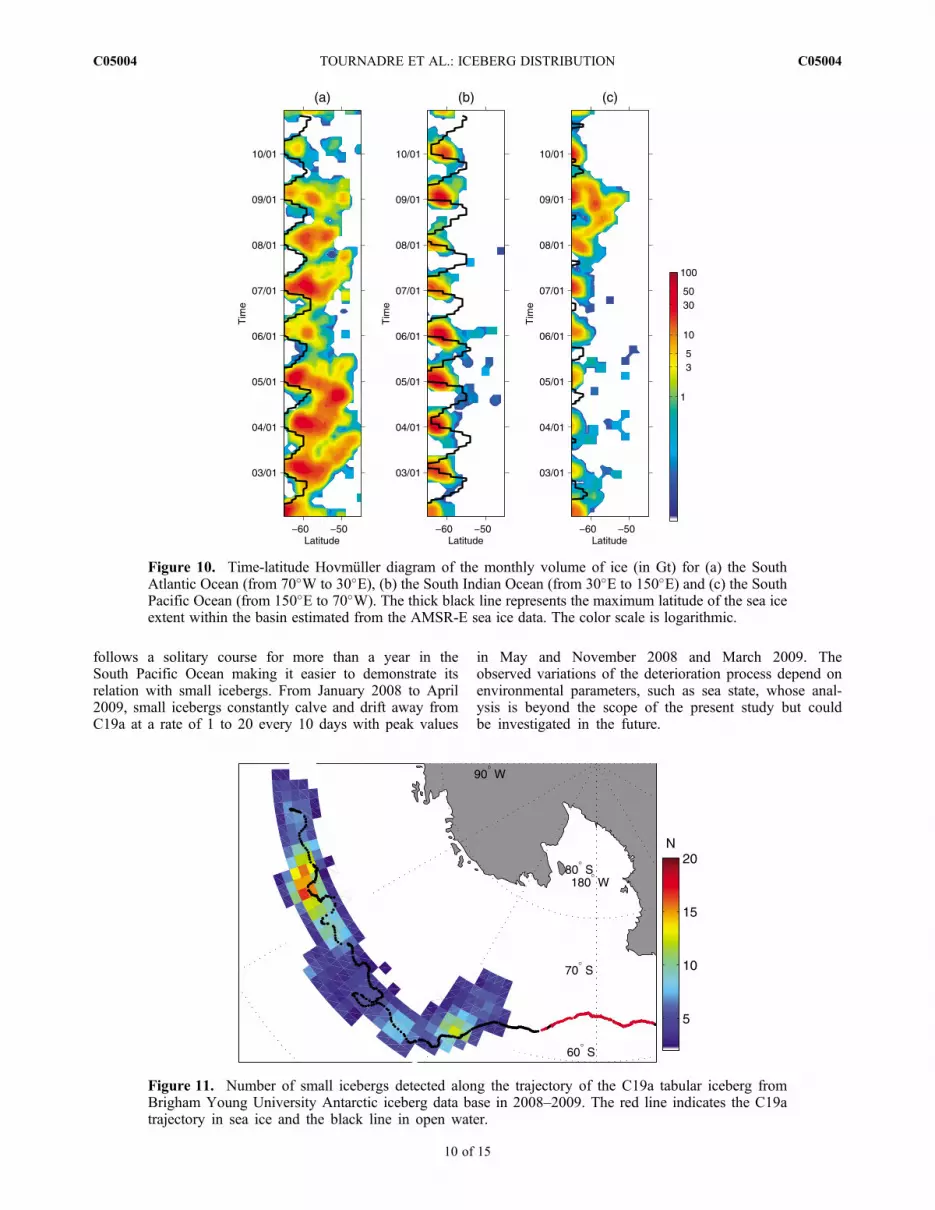
they can be used to analyze the transport of ice. The time-longitude diagram of the volume of ice integrated between66�S and 45�S presented in Figure 9 reveals the release oficebergs trapped in sea ice at the beginning of the australsummer in December-January. The position of the zone ofrelease, as well as the volume of ice, are highly variable inthe three basins. For example, in the SI (50 to 150�W), thiszone covers 83 degrees of longitude (from 47�W to 120�W)with a maximum of 20 Gt in 2003 and reduces about 40degrees (from 70�W to 110�W) in 2010 with a maximum of4 Gt. Some regions like the Bellinghausen Sea (�90�W), arecharacterized by small sporadic bursts of icebergs (in 2005).The overall pattern of the distribution reveals a generaleastward propagation of icebergs in the three basins. Thispropagation is particularly visible when icebergs are presentin open water during winter and thus travel quite far northwithin the ACC or the Wedell or Ross Gyres, such as in2003 to 2005 in the SA or in 2008–2009 in the SP. For theseyears, the eastward transport appears significantly faster inthe SP than that in the SA.[31] The time-latitude Hovmüller diagram of the monthly

volume of ice in the three ocean basins, presented inFigure 10, confirms the complexity and high variability oficeberg distribution. Except in the SI and SP oceans, ice-bergs are present only sporadically in open water in winter.

In the SA, large amounts of ice are not re-trapped by sea iceand can travel north, as far as 45�N (in 2003 and 2004).During the austral summer, the apparent southward transportof ice reflects the southwards retreat of sea ice that freestrapped icebergs. In the SA, large amounts of ice areadvected to the north especially in 2003, 2004 and 2007.This northward advection is in general quite limited in thetwo other ocean basins except sporadically like in 2008–2009 in the SP and 2005–2006 in the SI.

4. Relation With Large Icebergs

[32] Although small icebergs calve from the Antarcticcontinent glaciers or are released by sea ice, a large pro-portion of those detected in open water results from thedeterioration of large icebergs, mainly tabular ones. Thiscalving of smaller icebergs from large ones can be clearlyseen on many satellite visible images and it is also manifestin Figure 11 that presents the trajectory of the C19a tab-ular iceberg and the number of coincident small icebergsin its vicinity. The C19a track comes from the BrighamYoung University Antarctic iceberg data base, whichprovides the location of icebergs larger than 5–6 km inlength [Stuart and Long, 2011b]. C19a was chosenbecause once released from sea ice in January 2008 it

Figure 9. Longitude-time Hovmüller diagram of the monthly volume of ice integrated from 66�S to50�S. The color scale is logarithmic.

TOURNADRE ET AL.: ICEBERG DISTRIBUTION C05004C05004

9 of 15

follows a solitary course for more than a year in theSouth Pacific Ocean making it easier to demonstrate itsrelation with small icebergs. From January 2008 to April2009, small icebergs constantly calve and drift away fromC19a at a rate of 1 to 20 every 10 days with peak values

in May and November 2008 and March 2009. Theobserved variations of the deterioration process depend onenvironmental parameters, such as sea state, whose anal-ysis is beyond the scope of the present study but couldbe investigated in the future.

Figure 10. Time-latitude Hovmüller diagram of the monthly volume of ice (in Gt) for (a) the SouthAtlantic Ocean (from 70�W to 30�E), (b) the South Indian Ocean (from 30�E to 150�E) and (c) the SouthPacific Ocean (from 150�E to 70�W). The thick black line represents the maximum latitude of the sea iceextent within the basin estimated from the AMSR-E sea ice data. The color scale is logarithmic.

Figure 11. Number of small icebergs detected along the trajectory of the C19a tabular iceberg fromBrigham Young University Antarctic iceberg data base in 2008–2009. The red line indicates the C19atrajectory in sea ice and the black line in open water.

TOURNADRE ET AL.: ICEBERG DISTRIBUTION C05004C05004

10 of 15

[33] Using the B.Y.U data base, the distance between smallicebergs and the nearest coincident large iceberg (>5 km inlength) was computed. The cumulative probability of thedistance, presented in Figure 12, shows that only 22% ofsmall icebergs are within 200 km from a large one and that50% are distanced at more than 500 km . The geographicaldistribution of the proportion of small icebergs closer than200 km to a large one as well as the mean distance, presentedin Figure 13, reveals two distinct regimes in the relationshipbetween small and large icebergs. The first one found in theScotia Sea (between the Antarctic Peninsula and the SouthGeorgia Island), along the Antarctic coast in the SI ocean,and in the SP around 60�S, is characterized by the proximitybetween small and large icebergs, indicating that in theseareas the small icebergs either calved from the large ones orin the same regions of Antarctica, then drift along similarpaths.[34] The second regime shows no direct relationship

between the small and large icebergs. No small icebergs arecloser than 200 km from a large one and the mean distance islarger than 800 km. This regime corresponds to transport ofice due solely to small icebergs drifting over very long dis-tances from their calving sources. For the 2002–2010 period,this is the exclusive regime for the eastern branch of theWedell Gyre where no large icebergs are detected.

[35] The time-longitude diagram of the monthly propor-tion of icebergs whose distance to a large iceberg is smallerthan 200 km (see Figure 14), also clearly shows the tworegimes, and allows a clearer understanding of some of theice distribution patterns observed in Figures 8–10. The largevolume of ice observed in the SP north of 58�S in 2008–2009 results from the deterioration of the C19a and B15atabular icebergs that drifted north and were caught in theACC. Similarly, the trajectories of the A38-A and B tabularicebergs and in particular their grounding in January 2004north east of South Georgia and their subsequent breakinginto several pieces [Jansen et al., 2005] explain the highconcentration of small icebergs observed in 2004 to the eastof South Georgia. The diagram also shows that the smallicebergs follows a diffusive process dispersing ice overmuch larger areas of the southern ocean than the large ones.[36] However, the relation between small iceberg s vol-

ume of ice and the monthly number of large icebergs in openwater (presented in Figure 15) is not straightforward. Forexample, while the number of large icebergs is above normalin 2008, especially during winter, the volume of small ice-berg ice is one of the lowest of the 2002–2010 period. On thecontrary, the lowest number of large icebergs is detected in2006, characterized by a volume of ice almost double that of2008. There might exist a more direct relationship but the

Figure 12. Proportion of the detected small icebergs closer than a given distance to the closest largeiceberg.

Figure 13. (a) Proportion of the small detected icebergs closer than 200 km to a large one and (b) meandistance of small icebergs to the closest large iceberg.

TOURNADRE ET AL.: ICEBERG DISTRIBUTION C05004C05004

11 of 15

pertinent parameters to analyze should be the volume of iceof the large icebergs, which is not yet routinely available.[37] A method has been proposed by Stuart and Long

[2011a] to estimate the size of large icebergs using Sea-Winds data and in the future it will be possible to estimatethe volume of large icebergs and analyze more precisely therelationship between small and large icebergs. Current

progress with for example the Cryosat altimetry should alsoallow more systematic freeboard surveys of these icebergs.

5. Fresh Water Flux

[38] The transport of ice by small icebergs could represent,as mentioned earlier, about 40% of the volume of ice

Figure 14. Longitude-time diagram integrated between 66�S and 50�S of the monthly mean proportionof small icebergs closer than 200 km to a large one. The black lines represents the trajectories of the BYUlarge icebergs in open water during the period.

Figure 15. Monthly mean number of large icebergs from 2002 to 2010 in the South Atlantic Ocean (redline), the South Indian (green line), the South Pacific (blue) line and the southern ocean (black line).

TOURNADRE ET AL.: ICEBERG DISTRIBUTION C05004C05004

12 of 15

transported by icebergs and could thus have a significantrole in the injection of fresh water in the ocean. The trackingof small icebergs is not possible using our iceberg data baseand it is thus not yet possible to estimate the melting rate ofindividual icebergs or the associated fresh water flux.However, as the icebergs detected are small (50% aresmaller than 380 m length), their half-life should be of theorder of 200 days according to Jacka and Giles [2007] andthus most of the ice detected in open water will most prob-ably melt within a year. The difference between the maxi-mum and minimum of the volume of ice observed duringone year can thus be considered as a proxy to the availablefresh water. This can give an insight to the regions of thesouthern ocean where fresh water is injected. It can also beused for comparison with model results such as the onesfrom Gladstone et al. [2001], Silva et al. [2006] and Martinand Adcroft [2010].[39] Compared to the hundred year average of fresh water

flux in the southern ocean presented by Martin and Adcroft[2010] using a coupled climate model including icebergs upto 2.2 km length, the distribution of the mean available freshwater presented in Figure 16 has the same range of valuesand overall patterns (see their Figure 2). However, in the SA,the flux in the Scotia Sea, the north-eastward transport bythe ACC and the recirculation within the eastern branchof the Wedell Gyre are significantly larger in our estimate. Inthe SP and SI oceans, the overall patterns of the two dis-tributions are quite similar but the northward transport of icenorth of 66�S is one order of magnitude larger in our field.[40] Similar results can be obtained by making a compar-

ison with the model results of Gladstone et al. [2001], Silvaet al. [2006] or Jongma et al. [2009], in particular, theunderestimation of the Wedell Gyre recirculation or of thenorthward transport in the SP and SI oceans.

6. Conclusion and Perspective

[41] The method presented by Tournadre et al. [2008] todetect small icebergs in open water using high resolution

altimeter waveforms has been improved to allow, assumingconstant iceberg freeboard elevation and ice backscattercoefficient, the estimate of the iceberg area as well as thevolume of ice and has been used to create a data base ofmore than 52,000 small icebergs covering the 2002–2010period, i.e., the whole Jason-1 archive. The distribution oficeberg size and length follow a lognormal distribution inagreement with previous studies on the distribution of ice-berg size based on ship-borne radars such as the one used byWadhams [1988]. The best fit of this lognormal distributiongives a mean iceberg length of 630 m within the mean lengthgiven by Romanov et al. [2011] for different iceberg shapesand somewhat larger than the mean value of 513 m given byWadhams [1988]. The iceberg size has a strong seasonalcycle reflecting the melting of icebergs during the australsummer that has been estimated at 1.5 m/day.[42] The total volume of ice in the southern ocean has an

estimated annual mean of about 400 Gt with an uncertaintyof 25–30%. This represents about 35% of the volume oflarge tabular icebergs given by Silva et al. [2006] and it canthus play a significant role in the injection of meltwater inthe ocean. The altimeter data allow to estimate the distribu-tion of ice volume with unprecedented spatial and temporalresolutions revealing small scale structures and sporadicevents such as the eastern Wedell Gyre recirculation or ice-berg production in the Mertz Glacier area. They also showthat the seasonal cycle of the volume of ice has a very highspatial and temporal inter-annual variability and this vari-ability is much contrasted between the three ocean basins(South Atlantic, Indian and Pacific oceans). The small ice-berg variability is at least partly due to the variability of largeicebergs distribution and travel. Some events like the pres-ence of the C19a and B15a icebergs in the South Pacificnorth of 60�S explains the anomalously high content of icein this region in 2008 and 2009. However, the analysis of therelationship between small and large icebergs clearly revealstwo different regimes, the first one characterized by theproximity of the two types of iceberg, corresponds to themain iceberg Alley or specific events where small icebergs(calved or not from large ones) and large ones travel inconvoy along the same path. In such a regime, the smallicebergs can be considered as diffusers of the ice containedin the large ones. The second one shows no or little relationbetween the two types and corresponds to a transport of iceover vast regions (for example the eastern branch of theWedell Gyre or the eastern South Pacific ocean) and longdistances solely by smaller icebergs. The lack of clear rela-tion between the number of large icebergs present in openwater and the volume of ice which shows that it is necessaryto have an estimate of the size of the large ones (not yetavailable on an operational basis) to further investigate thesmall/large iceberg relationship.[43] The small iceberg data set can not yet be used to

track individual icebergs and it is thus not possible toestimate directly the melting rate or the associated freshwater flux. However, as the considered icebergs are smalland have a half-life of the order of 200 days, the differ-ence between the annual maximum and minimum of thevolume of ice can be seen as a proxy to the available freshwater. The comparison with results from numerical modelsincluding iceberg drift and melting shows a good overallagreement of the patterns of the distribution and the range

Figure 16. Mean annual available fresh water in mm.yr�1.The gray scale is logarithmic.

TOURNADRE ET AL.: ICEBERG DISTRIBUTION C05004C05004

13 of 15

of value. However, in the SA, the flux in the Scotia Sea,the north-eastward transport by the ACC and the recircu-lation within the eastern branch of the Wedell Gyre arelarger in our estimate.[44] Small icebergs can therefore play a significant role in

the transport of ice in the southern ocean, diffusing the ice ofthe large icebergs or of the Antarctic continent over largeregions and over vast distances and should be taken intoaccount for climatological, physical or biological oceanog-raphy studies.[45] In the near future, we plan to increase the size of the

small iceberg data base by adapting the method to otheraltimeters (ERS-1 and 2, Topex-Poseidon, Envisat andJason-2) and make it available to the community. This willenable the analysis of the evolution of small icebergs overalmost 20 years, once the homogeneity and consistency ofthe detection by the different altimeter is tested and vali-dated. The data set can also be used to study the possibleimpact of small icebergs on the physical and biologicalproperties of the southern ocean.

Appendix A: Detection Method

[46] The detection method used in the present study is adevelopment of the one presented by Tournadre et al.[2008]. It is summarized here. An altimeter is a nadir look-ing radar that emits short pulses that are backscattered by thesea surface. The altimeter measures the backscattered poweras a function of time to construct the echo waveform fromwhich the geophysical parameters are estimated. The back-scatter coefficient of the waveform can be expressed as adouble convolution product of the radar point targetresponse, the flat sea surface response and the joint proba-bility density function of slope and elevation of the seasurface [Brown, 1977]. The radar cross section for back-scatter as a function of time, s(t), assuming a Gaussianaltimeter pulse, a Gaussian antenna pattern and a Gaussianrandom distribution of rough-surface specular points, can beexpressed as [Barrick and Lipa, 1985]

s tð Þ ¼ 1

22pð Þ3=2H″sts0 1þ erf

xffiffiffi2

psp

! !e�

xub ; ðA1Þ

where x = ct/2, H″ = H/(1 + H/a) is the reduced satelliteheight, a being the earth’s radius, and H the satellite height.st is the standard deviation of the altimeter pulse; sp ¼ffiffiffiffiffiffiffiffiffiffiffiffiffiffiffih2 þ s2

t

pwhere h is the RMS wave height; ub is the

antenna pattern standard deviation; s0 is the target back-scatter coefficient. It should be noted that t = 0 correspondsto the mean sea level. The measured Jason-1 waveforms aregiven in telemetry samples of 3.125 ns width (the length ofthe pulse) and the nominal track point (i.e., the sea levelor t = 0) is shifted to bin 32.5.[47] A point target of height d above sea level located at

distance d from the satellite nadir will give an echo at thetime t0 defined by [Powell et al., 1993]

ct02

¼ �d þ 1

2

aþ H

aHd2 ¼ �d þ d2

2H″: ðA2Þ

The echo waveform of a point target is purely deterministic,i.e., a parabola as a function of time. Using the radar equa-tion [Roca et al., 2003] it is of the form

starget tð Þ ¼ s1

2p2H4 1þ d22H2

� � e�u0ub e

� xþd�u0ð Þ22s2t ; ðA3Þ

where s1 is the target radar cross section, and u0 ¼ d2

2H ″.[48] For an iceberg of area A and constant surface back-

scatter coefficient s1, the waveform is obtained by summa-tion of (9) over A

sice tð Þ ¼ s1

2p2H4

IA

1

1þ d22H2

e�u0ub e

� xþd�u0ð Þ22s2t dA: ðA4Þ

To be detectable in echo waveforms, an iceberg should havean echo at a time, t0 that lies within the time range duringwhich the echo waveform is integrated, i.e., for Jason-1between the telemetry sample 1 and 30. The target back-scatter coefficient should also be large enough to come outof the thermal noise of the sensor. This noise, estimated overmore than 10 million waveforms has a mean value �8.5 dBwith a standard deviation of 1.3 dB. The backscatter ofan iceberg has to be larger than �4.6 dB to come out ofthe thermal noise at a 3 std level. For icebergs larger than thealtimeter footprint (�8–10 km2, i.e., length > 3 km), thechange in surface elevation and the significant modificationof the waveform shape is too rapid and causes the altimetertracker to lose lock resulting in the loss of data for severalseconds [Hawkins et al., 1991].

A1. Iceberg Detection

[49] The signature of icebergs is always characterized bythe parabolic shape defined by (8). The automated detectionis based on the analysis of the convolution product Cbetween a filter, F characteristic of an iceberg signature, andthe thermal noise sections of the waveforms

C i; jð Þ ¼X30n¼1

XM2

m¼1

s0 i; jð ÞF i� n; j� mð Þ; ðA5Þ

where i is the telemetry sample index, j, the waveformindex, and s0(i, j), the jth waveform. The filter used hasbeen computed by the waveform model of (10) for a100 � 100 m2 iceberg.[50] For each waveform, the maximum of correlation C( j)

and its location imaxC ( j) (i.e., the range), and the maximum of

backscatter, smax( j) and its location imaxs ( j) are determined. A

waveform is assumed to contain an iceberg signature ifCmax( j) and smax( j) are larger than given thresholds C1 ands1.[51] For each signature a maximum of 40 waveforms can

be involved [Tournadre et al., 2008]. If n consecutivewaveforms are detected as containing a signature, the time ofthe echo (tech) is estimated as

tech ¼ 32:5�min ismax jð Þ; j ¼ 1::n� �� �

∗ 3:125 ðA6Þ

and the iceberg backscatter, siceb, is estimated as the maxi-mum observed backscatter of the whole signature, i.e.,

siceb ¼ max smax jð Þ; j ¼ 1::nð Þ: ðA7Þ

TOURNADRE ET AL.: ICEBERG DISTRIBUTION C05004C05004

14 of 15

[52] Acknowledgments. The large iceberg data base used in thisstudy is produced by the Brigham Young University, Center for RemoteSensing, and is available at http://www.scp.byu.edu/data/iceberg/. TheAMSR-E data sea ice concentration data are produced by the Universityof Bremen under the GMES project Polar View and are available athttp://iup.physik.uni-bremen.de:8084/amsredata/asidaygridswath/l1a/s6250/.The CLS AVISO operation center generously supplied us with the Jason-1sensor geophysical data record (SGDR). The authors also want to acknowl-edge financial support by the Centre National d’Etudes Spatiales (TOSCAprogram).

ReferencesBarrick, D., and B. Lipa (1985), Analysis and interpretation of altimeter seaecho, in Satellite Oceanic Remote Sensing, Adv. Geophys. Ser., vol. 27,edited by B. Saltzman, pp. 61–100, Academic, Orlando, Fla.

Brown, G. S. (1977), The average impulse response of a rough surface andits applications, IEEE Trans. Antennas Propag., 25, 67–74.

Dowdeswell, J. A., and J. L. Bamber (2007), Keel depths of modern Antarc-tic icebergs and implications for sea-floor scouring in the geologicalrecord, Mar. Geol., 243, 120–131,doi:10.1016/j.margeo.2007.04.008.

Faugère, Y., J. Dorandeu, F. Lefevre, N. Picot, and P. Féménias (2006),Envisat ocean altimetry performance assessment and cross-calibration,Sensors, 6, 100–130.

Gladstone, R., and G. Bigg (2002), Satellite tracking of icebergs in the Wed-dell Sea, Antarct. Sci., 14, 278–287, doi:10.1017/S0954102002000032.

Gladstone, R. M., G. R. Bigg, and K. W. Nicholls (2001), Iceberg trajectorymodeling and meltwater injection in the Southern Ocean, J. Geophys.Res., 106, 19,903–19,916, doi:10.1029/2000JC000347.

Glasby, G. P. (Ed.) (1990), Antarctic Sector of the Pacific, 396 pp., Elsevier,Amsterdam.

Hawkins, J., S. Laxon, and H. Phillips (1991), Antarctic tabular icebergmulti-sensor mapping, in International Geoscience and Remote SensingSymposium, 1991. IGARSS ’91. Remote Sensing: Global Monitoring forEarth Management, vol. 3, edited by Inst. of Electr. and Electron. Eng.Ed., pp. 1605–1608, New York.

Horn, P. S. (1990), Robust quantile estimators for skewed populations,Biometrika, 77, 631–636.

Jacka, T. H., and A. B. Giles (2007), Antarctic iceberg distribution and dis-solution from ship-based observations, J. Glaciol., 53, 341–356.

Jansen, D., H. Sandh ager, and W. Rack (2005), Evolution of tabular ice-berg A-38B, obsevation and simulation, FRISP Rep. 16, Alfred WegenerInst., Helgoland, Germany.

Jongma, J. I., E. Driesschaert, T. Fichefet, H. Goosse, and H. Renssen(2009), The effect of dynamic-thermodynamic icebergs on the SouthernOcean climate in a three-dimensional model, Ocean Modell., 26(1–2),104–113, doi:10.1016/j.ocemod.2008.09.007.

Keys, J., and D. Fowler (1989), Sources and movement of icebergs in thesouth-west Ross Sea, Antarctica, Ann. Glaciolog., 12, 85–88.

Klatt, O., E. Fahrbach, M. Hoppema, and G. Rohardt (2005), The transportof the Weddell Gyre across the prime meridian, Deep Sea Res., Part II,52(3–4), 513–528, doi:10.1016/j.dsr2.2004.12.015.

Lancelot, C., A. de Montety, H. Goosse, S. Becquevort, V. Schoemann,B. Pasquer, and M. Vancoppenolle (2009), Spatial distribution of theiron supply to phytoplankton in the Southern Ocean: A model study,Biogeosciences, 6, 2861–2878.

Legrésy, B., F. Papa, F. Rémy, G. Vinay, M. Van den Bosch, and O.-Z.Zanife (2005), Envisat radar altimeter measurements over continental sur-faces and ice caps using the ICE-2 retracking algorithm, Remote Sens.Environ., 95, 150–163.

Long, D., J. Ballantyne, and C. Bertoia (2002), Is the number of Antarcticicebergs really increasing?, Eos Trans. AGU, 83(42), 469, 474.

Martin, T., and A. Adcroft (2010), Parameterizing the fresh-water flux fromland ice to ocean with interactive icebergs in a coupled climate model,Ocean Modell., 34(3–4), 111–124, doi:10.1016/j.ocemod.2010.05.001.

Ménard, Y., and L. Fu (2001), Jason-1 mission, Aviso Newsl., 8, 4–9.

Powell, R. J., A. R. Birks, W. J. Bradford, C. L. Wrench, and J. Biddiscombe(1993), Using transponders with ERS1-1 and Topex altimeters to measureorbit altitude to �3 cm, Adv. Space Res., 13, 61–67.

Raiswell, R., L. G. Benning, M. Tranter, and S. Tulaczyk (2008), Bioavail-able iron in the Southern Ocean: The significance of the iceberg conveyorbelt, Geochem. Trans., 9, 1–23, doi:10.1186/1467-4866-9-7.

Roca, M., H. Jackson, and C. Celani (2003), RA-2 sigma-0 absolute calibra-tion, paper presented at EGS-AGU-EUG Joint Assembly, Nice, France,6–11 Apr.

Romanov, Y. A., N. A. Romanova, and P. Romanov (2008), Distribution oficebergs in the Atlantic and Indian Ocean sectors of the Antarctic regionand its possible links with ENSO, Geophys. Res. Lett., 35, L02506,doi:10.1029/2007GL031685.

Romanov, Y. A., N. A. Romanova, and P. Romanov (2011), Shape and sizeof Antarctic icebergs derived from ship observation data, Antarct. Sci.,24, 77–87, doi:10.1017/S0954102011000538.

Schodlok, M. P., H. H. Hellmer, G. Rohardt, and E. Fahrbach (2006),Weddell Sea iceberg drift: Five years of observations, J. Geophys.Res., 111, C06018, doi:10.1029/2004JC002661.

Schwarz, J. N., and M. P. Schodlok (2009), Impact of drifting icebergson surface phytoplankton biomass in the Southern Ocean: Ocean col-our remote sensing and in situ iceberg tracking, Deep Sea Res., Part I,56(10), 1727–1741, doi:10.1016/j.dsr.2009.05.003.

Silva, T., and G. Bigg (2005), Computer-based identification and trackingof Antarctic icebergs in sar images, Remote Sens. Envir., 94, 287–297,doi:10.1016/j.rse.2004.10.002.

Silva, T., G. Bigg, and K. Nicholls (2006), The contribution of giant ice-bergs to the Southern Ocean freshwater flux, J. Geophys. Res., 111,C03004, doi:10.1029/2004JC002843.

Smith, K. L. (2011), Free-drifting icebergs in the Southern Ocean: An over-view, Deep Sea Res., Part II, 58(11–12), 1277–1284, doi:10.1016/j.dsr2.2010.11.003.

Soviet Antarctic Survey (1966), Antarctic Atlas, Moscow.Spreen, G., L. Kaleschke, and G. Heygster (2008), Sea ice remote sensingusing AMSR-E 89-GHz channels, J. Geophys. Res., 113, C02S03,doi:10.1029/2005JC003384.

Stuart, K., and D. Long (2011a), Iceberg size and orientation estimationusing seawinds, Cold Reg. Sci. Technol., 69, 39–51, doi:10.1016/j.coldregions.2011.07.006.

Stuart, K. M., and D. G. Long (2011b), Tracking large tabular icebergsusing the SeaWinds Ku-band microwave scatterometer, Deep Sea Res.,Part II, 58(11–12), 1285–1300, doi:10.1016/j.dsr2.2010.11.004.

Tchernia, P., and P. F. Jeannin (1984), Circulation in antarctic waters asrevealed by icebergs tracks 1972–1983, Polar Rec., 22, 263–269.

Tournadre, J. (2007), Signature of lighthouses, ships, and small islands inaltimeter waveforms, J. Atmos. Oceanic Technol., 24, 1143–1149.

Tournadre, J., K. Whitmer, and F. Girard-Ardhuin (2008), Iceberg detectionin open water by altimeter waveform analysis, J. Geophys. Res., 113,C08040, doi:10.1029/2007JC004587.

Tran, N., F. Rémy, H. Feng, and P. Féménias (2008), Snow facies over icesheets derived from Envisat active and passive observations, IEEE Trans.Geosci. Remote Sens., 46(11), 3694–3708.

Tran, N., F. Girard-Ardhuin, R. Ezraty, H. Feng, and P. Féménias (2009),Defining a sea ice flag for Envisat altimetry mission, IEEE Geosci.Remote Sens. Lett., 6, 77–81, doi:10.1109/LGRS.2008.2005275.

Wadhams, P. (1988), Winter observations of iceberg frequencies and sizesin the South Atlantic Ocean, J. Geophys. Res., 93, 3583–3590.

Wilks, D. (2006), Statistical Methods in the Atmospheric Sciences, 2nd ed.,Int. Geophys. Ser., vol. 59, 627 pp., Academic, Amsterdam.

Young, N. W. (1998), Antarctic iceberg drift and ocean current derivedfrom scatterometer image series, paper presented at Workshop on Emerg-ing Scatterometer Applications—From Research to Operations, Eur.Space Agency, Noordwijk, Netherlands, 5–7 Oct.

Young, N. W., D. Turner, G. Hyland, and R. N. Williams (1998), Nearcoastal iceberg distributions in east Antarctica, 50�E–145�E, Ann. Gla-ciol., 27, 68–74.

TOURNADRE ET AL.: ICEBERG DISTRIBUTION C05004C05004

15 of 15