Application of statistical physics to heartbeat diagnosis

Physica A 274 (1999) 99–110www.elsevier.com/locate/physa

Application of statistical physics toheartbeat diagnosis

S. Havlina;b;∗, L.A.N. Amaralb , Y. Ashkenazya , A.L. Goldbergerc ,P.Ch. Ivanovb;c , C.-K. Pengb;c , H.E. Stanleyb

aGonda-Goldschmied Center, Department of Physics, Bar-Ilan University, Ramat-Gan 52900, IsraelbCenter for Polymer Studies and Department of Physics, Boston University, Boston, MA 02215, USAcCardiovascular Division, Harvard Medical School, Beth Israel Hospital, Boston, MA 02215, USA

Abstract

We present several recent studies based on statistical physics concepts that can be used asdiagnostic tools for heart failure. We describe the scaling exponent characterizing the long-rangecorrelations in heartbeat time series as well as the multifractal features recently discovered inheartbeat rhythm. It is found that both features, the long-range correlations and the multifractility,are weaker in cases of heart failure. c© 1999 Elsevier Science B.V. All rights reserved.

1. The human heartbeat

It is common to describe the normal electrical activity of the heart as “regular sinusrhythm”. However, cardiac interbeat intervals uctuate in a complex, apparently erraticmanner in healthy subjects even at rest. Analysis of heart rate variability has focusedprimarily on short time oscillations associated with breathing (0:15–0:40 Hz) and bloodpressure control (∼ 0:1 Hz) [1]. Fourier analysis of longer heart-rate sets from healthyindividuals typically reveals a 1=f-like spectrum for frequencies ¡ 0:1 Hz [2–7].Peng et al. [8–10] studied scale-invariant properties of the human heartbeat time

series. The analysis is based on beat-to-beat heart rate uctuations over very long timeintervals (up to 24 h ≈ 105 beats) recorded with an ambulatory monitor. 1 The time

∗ Correspondence address: Gonda-Goldschmied Center, Department of Physics, Bar-Ilan University,Ramat-Gan 52900, Israel. Fax: +972-3-535-3298.E-mail address: [email protected] (S. Havlin)1 Heart Failure Database (Beth Israel Deaconess Medical Center, Boston, MA). The database includes 18healthy subjects (13 female and 5 male, with ages between 20 and 50, average 34.3 yr), and 12 congestiveheart failure subjects (3 female and 9 male, with ages between 22 and 71, average 60.8 yr) in sinus rhythm.

0378-4371/99/$ - see front matter c© 1999 Elsevier Science B.V. All rights reserved.PII: S 0378 -4371(99)00333 -7

100 S. Havlin et al. / Physica A 274 (1999) 99–110

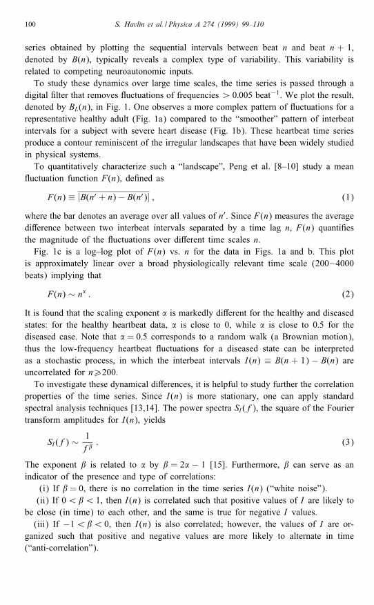
series obtained by plotting the sequential intervals between beat n and beat n + 1,denoted by B(n), typically reveals a complex type of variability. This variability isrelated to competing neuroautonomic inputs.To study these dynamics over large time scales, the time series is passed through a

digital �lter that removes uctuations of frequencies ¿ 0:005 beat−1. We plot the result,denoted by BL(n), in Fig. 1. One observes a more complex pattern of uctuations for arepresentative healthy adult (Fig. 1a) compared to the “smoother” pattern of interbeatintervals for a subject with severe heart disease (Fig. 1b). These heartbeat time seriesproduce a contour reminiscent of the irregular landscapes that have been widely studiedin physical systems.To quantitatively characterize such a “landscape”, Peng et al. [8–10] study a mean

uctuation function F(n), de�ned as

F(n) ≡ |B(n′ + n)− B(n′)| ; (1)

where the bar denotes an average over all values of n′. Since F(n) measures the averagedi�erence between two interbeat intervals separated by a time lag n, F(n) quanti�esthe magnitude of the uctuations over di�erent time scales n.Fig. 1c is a log–log plot of F(n) vs. n for the data in Figs. 1a and b. This plot

is approximately linear over a broad physiologically relevant time scale (200–4000beats) implying that

F(n) ∼ n� : (2)

It is found that the scaling exponent � is markedly di�erent for the healthy and diseasedstates: for the healthy heartbeat data, � is close to 0, while � is close to 0:5 for thediseased case. Note that � = 0:5 corresponds to a random walk (a Brownian motion),thus the low-frequency heartbeat uctuations for a diseased state can be interpretedas a stochastic process, in which the interbeat intervals I(n) ≡ B(n + 1) − B(n) areuncorrelated for n¿200.To investigate these dynamical di�erences, it is helpful to study further the correlation

properties of the time series. Since I(n) is more stationary, one can apply standardspectral analysis techniques [13,14]. The power spectra SI (f), the square of the Fouriertransform amplitudes for I(n), yields

SI (f) ∼ 1f�

: (3)

The exponent � is related to � by � = 2� − 1 [15]. Furthermore, � can serve as anindicator of the presence and type of correlations:

(i) If � = 0, there is no correlation in the time series I(n) (“white noise”).(ii) If 0¡�¡ 1, then I(n) is correlated such that positive values of I are likely to

be close (in time) to each other, and the same is true for negative I values.(iii) If −1¡�¡ 0, then I(n) is also correlated; however, the values of I are or-

ganized such that positive and negative values are more likely to alternate in time(“anti-correlation”).

S. Havlin et al. / Physica A 274 (1999) 99–110 101

Fig. 1. The interbeat interval BL(n) after low-pass �ltering for (a) a healthy subject and (b) a patient withsevere cardiac disease (dilated cardiomyopathy). The healthy heartbeat time series shows more complex uctuations compared to the diseased heart rate uctuation pattern that is close to random walk (“brown”)noise. (c) Log–log plot of F(n) vs. n. The circles represent F(n) calculated from data in (a) and the trianglesfrom data in (b). The two best-�t lines have slope � = 0:07 and � = 0:49 (�t from 200 to 4000 beats).The two lines with slopes � = 0 and � = 0:5 correspond to “1=f noise” and “brown noise”, respectively.We observe that F(n) saturates for large n (of the order of 5000 beats), because the heartbeat interval aresubjected to physiological constraints that cannot be arbitrarily large or small. After Peng et al. [8–10].

For the diseased data set, we observe a at spectrum (� ≈ 0) in the low-frequencyregion con�rming that I(n) are not correlated over long time scales (low frequencies).In contrast, for the data set from the healthy subject we obtain � ≈ −1, indicatingnontrivial long-range correlations in B(n) – these correlations are not the consequence


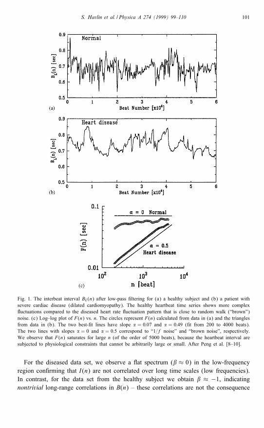
Fig. 2. Plot of logF(n) vs. log n for two long interbeat interval time series (∼24 h). The circles arefor a representative healthy subject while the triangles are from a subject with congestive heart failure.Arrows indicate “crossover” points in scaling. Note altered scaling with heart failure, suggesting apparentperturbations of both short and long-range correlation mechanisms. After Peng et al. [8–10].

of summation over random variables or artifacts of non-stationarity. Furthermore, the“anti-correlation” properties of I(n) indicated by the negative � value are consistentwith a nonlinear feed-back system that “kicks” the heart rate away from extremes. Thistendency, however, does not only operate on a beat-to-beat basis (local e�ect) but ona wide range of time scales.A further improvement to the study of the long-range correlation exponent � –

detrended uctuation analysis (DFA) – has been proposed and developed by Penget al. [11,12]. Fig. 2 compares the DFA analysis of representative 24 h interbeat in-terval time series of a healthy subject (©) and a patient with congestive heart failure(4). Note that for large time scales (asymptotic behavior), the healthy subject showsalmost perfect power-law scaling over more than two decades (206n610 000) with�DFA=1 (i.e., 1=f noise) while for the pathologic data set �DFA ≈ 1:3 (closer to Brow-nian noise). This result is consistent with our previous �nding [8–10] that there is asigni�cant di�erence in the long-range scaling behavior between healthy and diseasedstates.To study the alteration of long-range correlations with pathology, we analyzed cardiac

interbeat data from three di�erent groups of subjects: (i) 29 adults (17 male and 12female) without clinical evidence of heart disease (age range: 20–64 yr, mean 41),(ii) 10 subjects with fatal or near-fatal sudden cardiac death syndrome (age range:35–82 yr) and (iii) 15 adults with severe heart failure (age range: 22–71 yr; mean 56).Data from each subject contains approximately 24 h of ECG recording encompassing∼ 105 heartbeats.For the normal control group, we observed �DFA =1:00±0:10 (mean value ± S.D.).

These results indicate that healthy heart rate uctuations are anticorrelated and exhibit


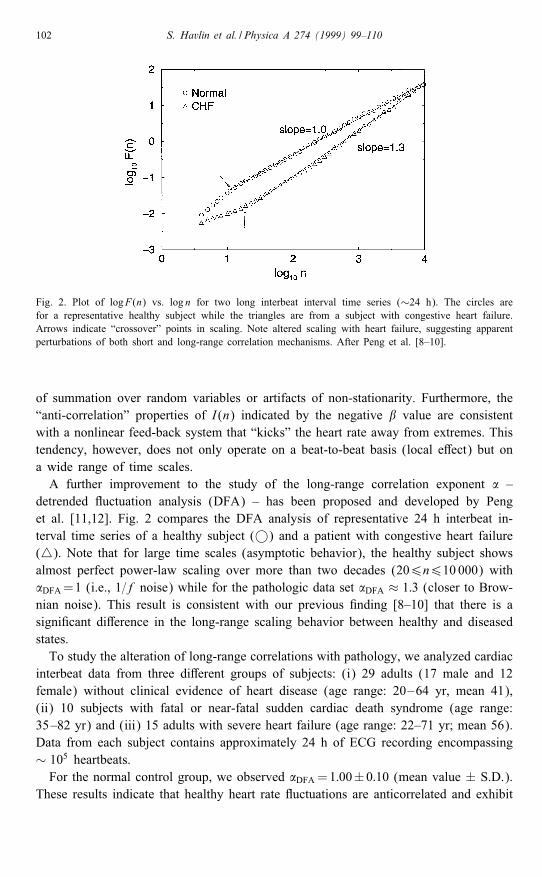
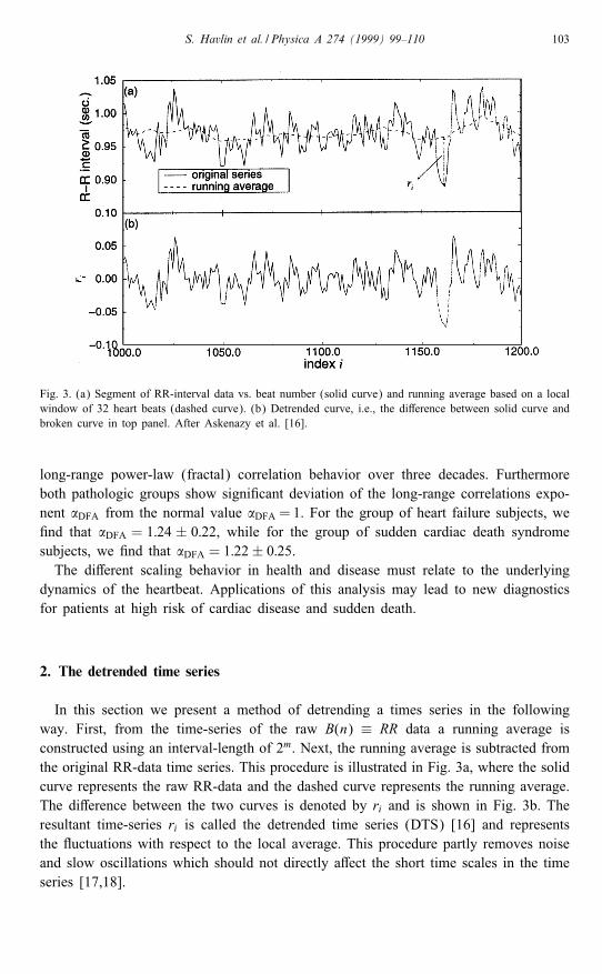
Fig. 3. (a) Segment of RR-interval data vs. beat number (solid curve) and running average based on a localwindow of 32 heart beats (dashed curve). (b) Detrended curve, i.e., the di�erence between solid curve andbroken curve in top panel. After Askenazy et al. [16].

long-range power-law (fractal) correlation behavior over three decades. Furthermoreboth pathologic groups show signi�cant deviation of the long-range correlations expo-nent �DFA from the normal value �DFA = 1. For the group of heart failure subjects, we�nd that �DFA = 1:24 ± 0:22, while for the group of sudden cardiac death syndromesubjects, we �nd that �DFA = 1:22± 0:25.The di�erent scaling behavior in health and disease must relate to the underlying

dynamics of the heartbeat. Applications of this analysis may lead to new diagnosticsfor patients at high risk of cardiac disease and sudden death.

2. The detrended time series

In this section we present a method of detrending a times series in the followingway. First, from the time-series of the raw B(n) ≡ RR data a running average isconstructed using an interval-length of 2m. Next, the running average is subtracted fromthe original RR-data time series. This procedure is illustrated in Fig. 3a, where the solidcurve represents the raw RR-data and the dashed curve represents the running average.The di�erence between the two curves is denoted by ri and is shown in Fig. 3b. Theresultant time-series ri is called the detrended time series (DTS) [16] and representsthe uctuations with respect to the local average. This procedure partly removes noiseand slow oscillations which should not directly a�ect the short time scales in the timeseries [17,18].


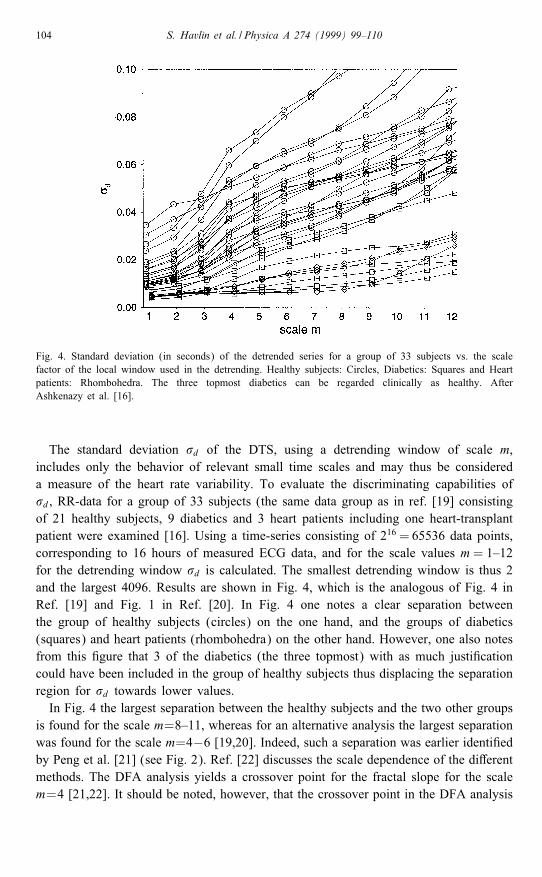
Fig. 4. Standard deviation (in seconds) of the detrended series for a group of 33 subjects vs. the scalefactor of the local window used in the detrending. Healthy subjects: Circles, Diabetics: Squares and Heartpatients: Rhombohedra. The three topmost diabetics can be regarded clinically as healthy. AfterAshkenazy et al. [16].

The standard deviation �d of the DTS, using a detrending window of scale m,includes only the behavior of relevant small time scales and may thus be considereda measure of the heart rate variability. To evaluate the discriminating capabilities of�d, RR-data for a group of 33 subjects (the same data group as in ref. [19] consistingof 21 healthy subjects, 9 diabetics and 3 heart patients including one heart-transplantpatient were examined [16]. Using a time-series consisting of 216 = 65536 data points,corresponding to 16 hours of measured ECG data, and for the scale values m= 1–12for the detrending window �d is calculated. The smallest detrending window is thus 2and the largest 4096. Results are shown in Fig. 4, which is the analogous of Fig. 4 inRef. [19] and Fig. 1 in Ref. [20]. In Fig. 4 one notes a clear separation betweenthe group of healthy subjects (circles) on the one hand, and the groups of diabetics(squares) and heart patients (rhombohedra) on the other hand. However, one also notesfrom this �gure that 3 of the diabetics (the three topmost) with as much justi�cationcould have been included in the group of healthy subjects thus displacing the separationregion for �d towards lower values.In Fig. 4 the largest separation between the healthy subjects and the two other groups

is found for the scale m=8–11, whereas for an alternative analysis the largest separationwas found for the scale m=4−6 [19,20]. Indeed, such a separation was earlier identi�edby Peng et al. [21] (see Fig. 2). Ref. [22] discusses the scale dependence of the di�erentmethods. The DFA analysis yields a crossover point for the fractal slope for the scalem=4 [21,22]. It should be noted, however, that the crossover point in the DFA analysis


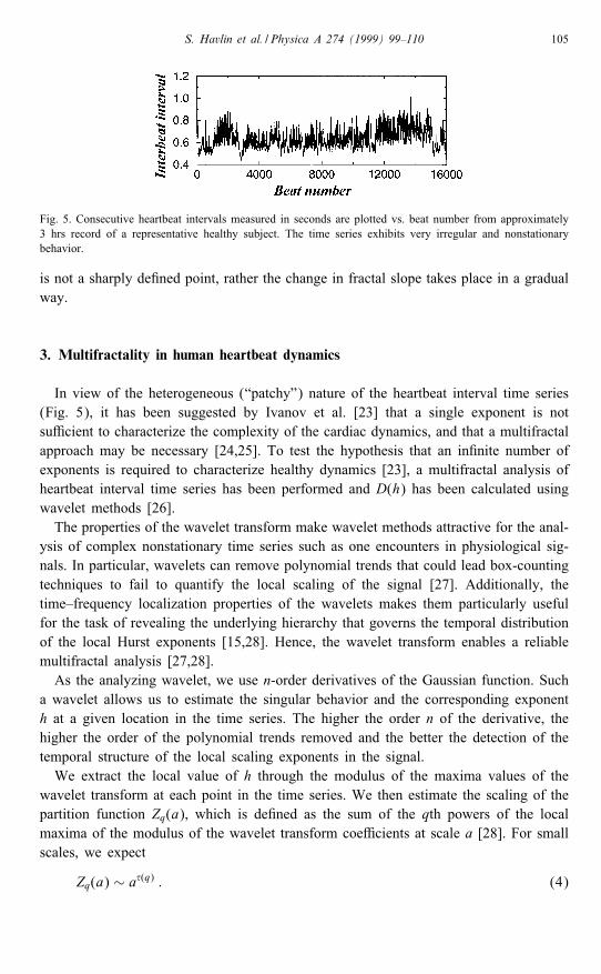
Fig. 5. Consecutive heartbeat intervals measured in seconds are plotted vs. beat number from approximately3 hrs record of a representative healthy subject. The time series exhibits very irregular and nonstationarybehavior.

is not a sharply de�ned point, rather the change in fractal slope takes place in a gradualway.

3. Multifractality in human heartbeat dynamics

In view of the heterogeneous (“patchy”) nature of the heartbeat interval time series(Fig. 5), it has been suggested by Ivanov et al. [23] that a single exponent is notsu�cient to characterize the complexity of the cardiac dynamics, and that a multifractalapproach may be necessary [24,25]. To test the hypothesis that an in�nite number ofexponents is required to characterize healthy dynamics [23], a multifractal analysis ofheartbeat interval time series has been performed and D(h) has been calculated usingwavelet methods [26].The properties of the wavelet transform make wavelet methods attractive for the anal-

ysis of complex nonstationary time series such as one encounters in physiological sig-nals. In particular, wavelets can remove polynomial trends that could lead box-countingtechniques to fail to quantify the local scaling of the signal [27]. Additionally, thetime–frequency localization properties of the wavelets makes them particularly usefulfor the task of revealing the underlying hierarchy that governs the temporal distributionof the local Hurst exponents [15,28]. Hence, the wavelet transform enables a reliablemultifractal analysis [27,28].As the analyzing wavelet, we use n-order derivatives of the Gaussian function. Such

a wavelet allows us to estimate the singular behavior and the corresponding exponenth at a given location in the time series. The higher the order n of the derivative, thehigher the order of the polynomial trends removed and the better the detection of thetemporal structure of the local scaling exponents in the signal.We extract the local value of h through the modulus of the maxima values of the

wavelet transform at each point in the time series. We then estimate the scaling of thepartition function Zq(a), which is de�ned as the sum of the qth powers of the localmaxima of the modulus of the wavelet transform coe�cients at scale a [28]. For smallscales, we expect

Zq(a) ∼ a�(q) : (4)


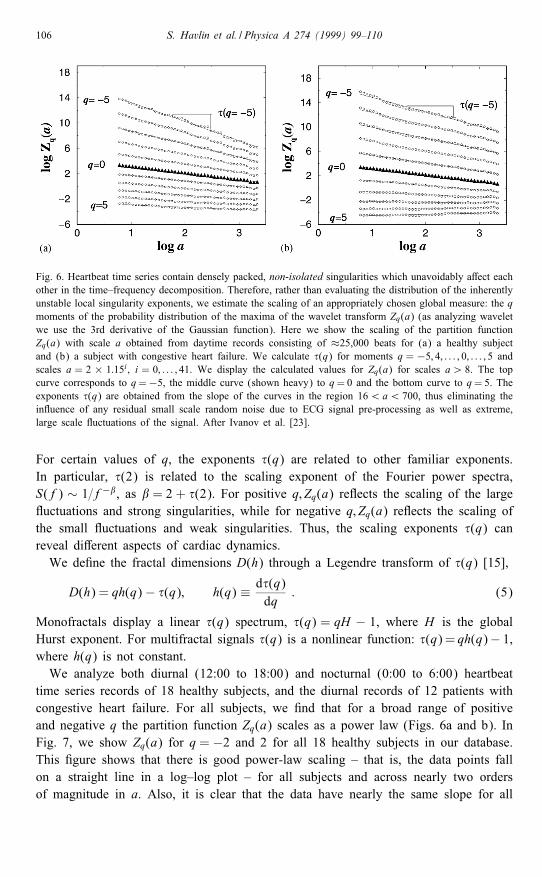
Fig. 6. Heartbeat time series contain densely packed, non-isolated singularities which unavoidably a�ect eachother in the time–frequency decomposition. Therefore, rather than evaluating the distribution of the inherentlyunstable local singularity exponents, we estimate the scaling of an appropriately chosen global measure: the qmoments of the probability distribution of the maxima of the wavelet transform Zq(a) (as analyzing waveletwe use the 3rd derivative of the Gaussian function). Here we show the scaling of the partition functionZq(a) with scale a obtained from daytime records consisting of ≈25,000 beats for (a) a healthy subjectand (b) a subject with congestive heart failure. We calculate �(q) for moments q = −5; 4; : : : ; 0; : : : ; 5 andscales a = 2 × 1:15i ; i = 0; : : : ; 41. We display the calculated values for Zq(a) for scales a¿ 8. The topcurve corresponds to q=−5, the middle curve (shown heavy) to q= 0 and the bottom curve to q= 5. Theexponents �(q) are obtained from the slope of the curves in the region 16¡a¡ 700, thus eliminating thein uence of any residual small scale random noise due to ECG signal pre-processing as well as extreme,large scale uctuations of the signal. After Ivanov et al. [23].

For certain values of q, the exponents �(q) are related to other familiar exponents.In particular, �(2) is related to the scaling exponent of the Fourier power spectra,S(f) ∼ 1=f−�, as � = 2 + �(2). For positive q; Zq(a) re ects the scaling of the large uctuations and strong singularities, while for negative q; Zq(a) re ects the scaling ofthe small uctuations and weak singularities. Thus, the scaling exponents �(q) canreveal di�erent aspects of cardiac dynamics.We de�ne the fractal dimensions D(h) through a Legendre transform of �(q) [15],

D(h) = qh(q)− �(q); h(q) ≡ d�(q)dq

: (5)

Monofractals display a linear �(q) spectrum, �(q) = qH − 1, where H is the globalHurst exponent. For multifractal signals �(q) is a nonlinear function: �(q)= qh(q)− 1,where h(q) is not constant.We analyze both diurnal (12:00 to 18:00) and nocturnal (0:00 to 6:00) heartbeat

time series records of 18 healthy subjects, and the diurnal records of 12 patients withcongestive heart failure. For all subjects, we �nd that for a broad range of positiveand negative q the partition function Zq(a) scales as a power law (Figs. 6a and b). InFig. 7, we show Zq(a) for q = −2 and 2 for all 18 healthy subjects in our database.This �gure shows that there is good power-law scaling – that is, the data points fallon a straight line in a log–log plot – for all subjects and across nearly two ordersof magnitude in a. Also, it is clear that the data have nearly the same slope for all


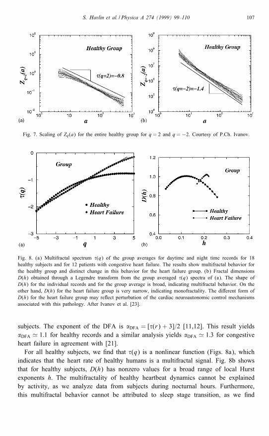
Fig. 7. Scaling of Zq(a) for the entire healthy group for q = 2 and q =−2. Courtesy of P.Ch. Ivanov.

Fig. 8. (a) Multifractal spectrum �(q) of the group averages for daytime and night time records for 18healthy subjects and for 12 patients with congestive heart failure. The results show multifractal behavior forthe healthy group and distinct change in this behavior for the heart failure group. (b) Fractal dimensionsD(h) obtained through a Legendre transform from the group averaged �(q) spectra of (a). The shape ofD(h) for the individual records and for the group average is broad, indicating multifractal behavior. On theother hand, D(h) for the heart failure group is very narrow, indicating monofractality. The di�erent form ofD(h) for the heart failure group may re ect perturbation of the cardiac neuroautonomic control mechanismsassociated with this pathology. After Ivanov et al. [23].

subjects. The exponent of the DFA is �DFA = [�(r) + 3]=2 [11,12]. This result yields�DFA ' 1:1 for healthy records and a similar analysis yields �DFA ' 1:3 for congestiveheart failure in agreement with [21].For all healthy subjects, we �nd that �(q) is a nonlinear function (Figs. 8a), which

indicates that the heart rate of healthy humans is a multifractal signal. Fig. 8b showsthat for healthy subjects, D(h) has nonzero values for a broad range of local Hurstexponents h. The multifractality of healthy heartbeat dynamics cannot be explainedby activity, as we analyze data from subjects during nocturnal hours. Furthermore,this multifractal behavior cannot be attributed to sleep stage transition, as we �nd


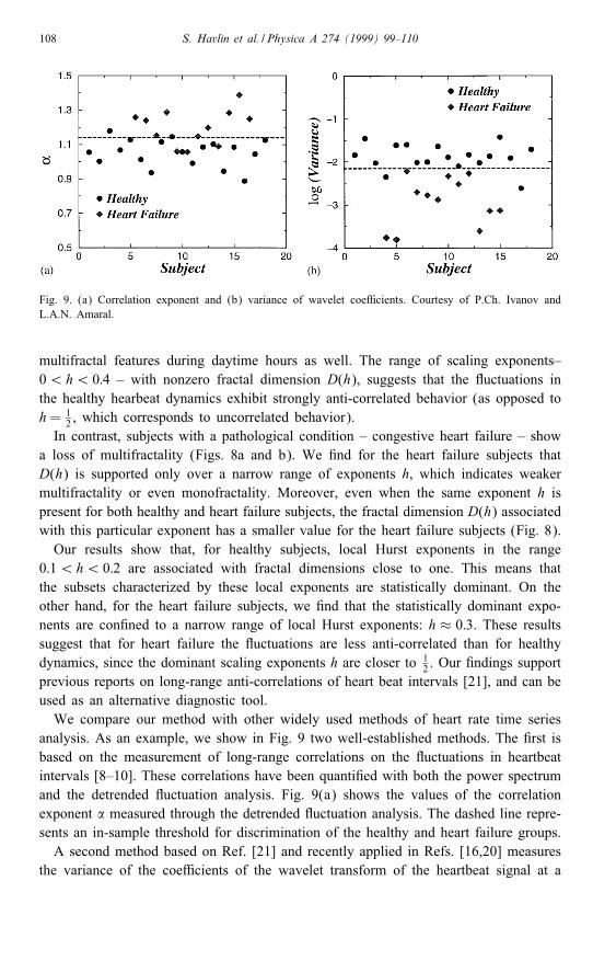
Fig. 9. (a) Correlation exponent and (b) variance of wavelet coe�cients. Courtesy of P.Ch. Ivanov andL.A.N. Amaral.

multifractal features during daytime hours as well. The range of scaling exponents–0¡h¡ 0:4 – with nonzero fractal dimension D(h), suggests that the uctuations inthe healthy hearbeat dynamics exhibit strongly anti-correlated behavior (as opposed toh= 1

2 , which corresponds to uncorrelated behavior).In contrast, subjects with a pathological condition – congestive heart failure – show

a loss of multifractality (Figs. 8a and b). We �nd for the heart failure subjects thatD(h) is supported only over a narrow range of exponents h, which indicates weakermultifractality or even monofractality. Moreover, even when the same exponent h ispresent for both healthy and heart failure subjects, the fractal dimension D(h) associatedwith this particular exponent has a smaller value for the heart failure subjects (Fig. 8).Our results show that, for healthy subjects, local Hurst exponents in the range

0:1¡h¡ 0:2 are associated with fractal dimensions close to one. This means thatthe subsets characterized by these local exponents are statistically dominant. On theother hand, for the heart failure subjects, we �nd that the statistically dominant expo-nents are con�ned to a narrow range of local Hurst exponents: h ≈ 0:3. These resultssuggest that for heart failure the uctuations are less anti-correlated than for healthydynamics, since the dominant scaling exponents h are closer to 1

2 . Our �ndings supportprevious reports on long-range anti-correlations of heart beat intervals [21], and can beused as an alternative diagnostic tool.We compare our method with other widely used methods of heart rate time series

analysis. As an example, we show in Fig. 9 two well-established methods. The �rst isbased on the measurement of long-range correlations on the uctuations in heartbeatintervals [8–10]. These correlations have been quanti�ed with both the power spectrumand the detrended uctuation analysis. Fig. 9(a) shows the values of the correlationexponent � measured through the detrended uctuation analysis. The dashed line repre-sents an in-sample threshold for discrimination of the healthy and heart failure groups.A second method based on Ref. [21] and recently applied in Refs. [16,20] measures

the variance of the coe�cients of the wavelet transform of the heartbeat signal at a


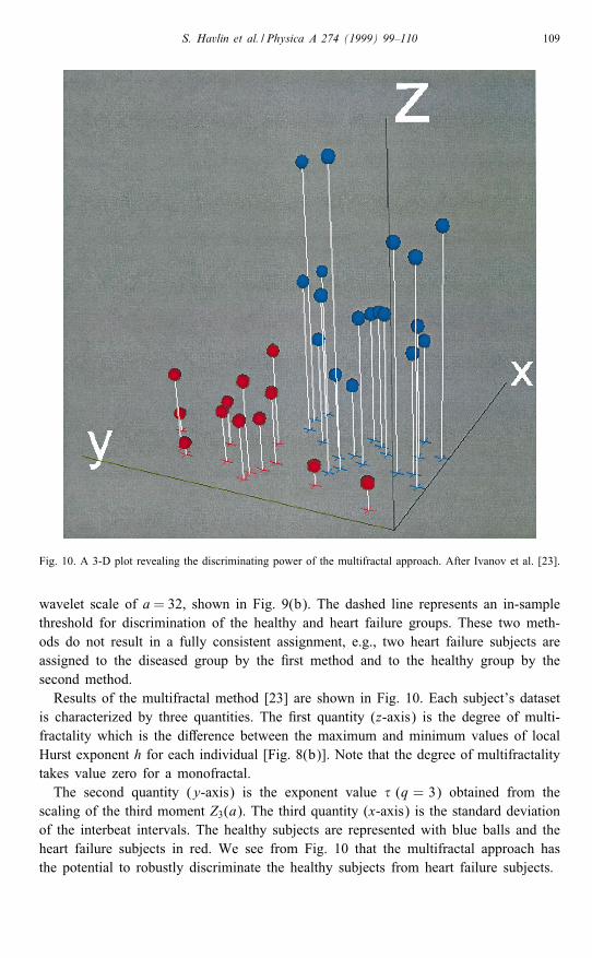
Fig. 10. A 3-D plot revealing the discriminating power of the multifractal approach. After Ivanov et al. [23].

wavelet scale of a= 32, shown in Fig. 9(b). The dashed line represents an in-samplethreshold for discrimination of the healthy and heart failure groups. These two meth-ods do not result in a fully consistent assignment, e.g., two heart failure subjects areassigned to the diseased group by the �rst method and to the healthy group by thesecond method.Results of the multifractal method [23] are shown in Fig. 10. Each subject’s dataset

is characterized by three quantities. The �rst quantity (z-axis) is the degree of multi-fractality which is the di�erence between the maximum and minimum values of localHurst exponent h for each individual [Fig. 8(b)]. Note that the degree of multifractalitytakes value zero for a monofractal.The second quantity (y-axis) is the exponent value � (q = 3) obtained from the

scaling of the third moment Z3(a). The third quantity (x-axis) is the standard deviationof the interbeat intervals. The healthy subjects are represented with blue balls and theheart failure subjects in red. We see from Fig. 10 that the multifractal approach hasthe potential to robustly discriminate the healthy subjects from heart failure subjects.


Acknowledgement

Supported by the NIH/National Center for Research Resources (grant P41 13622).

References

[1] W.F. Doolittle, in: E. Stone, R. Schwartz (Eds.), Intervening Sequences in Evolution and Development,Oxford University Press, New York, 1990, p. 42.

[2] R.I. Kitney, O. Rompelman, The Study of Heart-Rate Variability, Oxford University Press, London,1980.

[3] S. Akselrod, D. Gordon, F.A. Ubel, D.C. Shannon, A.C. Barger, R.J. Cohen, Science 213 (1981) 220.[4] M. Kobayashi, T. Musha, IEEE Trans. Biomed. Eng. 29 (1982) 456.[5] A.L. Goldberger, D.R. Rigney, J. Mietus, E.M. Antman, S. Greenwald, Experientia 44 (1988) 983.[6] J.P. Saul, P. Albrecht, D. Berger, R.J. Cohen, Computers in Cardiology, IEEE Computers Society Press,

Washington DC, 1987, pp. 419–422.[7] D.T. Kaplan, M. Talajic, Chaos 1 (1991) 251.[8] C.-K. Peng, J.E. Mietus, J.M. Hausdor�, S. Havlin, H.E. Stanley, A.L. Goldberger, Phys. Rev. Lett. 70

(1993) 1343.[9] C.-K. Peng, Ph.D. Thesis, Boston University, 1993.[10] C.-K. Peng, S.V. Buldyrev, J.M. Hausdor�, S. Havlin, J.E. Mietus, M. Simons, H.E. Stanley, A.L.

Goldberger, in: G.A. Losa, T.F. Nonnenmacher, E.R. Weibel (Eds.), Fractals in Biology and Medicine,Birkhauser Verlag, Boston, 1994.

[11] C.-K. Peng, S.V. Buldyrev, S. Havlin, M. Simons, H.E. Stanley, A.L. Goldberger, Phys. Rev. E 49(1994) 1685.

[12] C.-K. Peng et al., J. Electrocardiol. 28 (1995) 59.[13] A. Bunde, S. Havlin (Eds.), Fractals and Disordered Systems, Springer, Berlin, 1991.[14] A. Bunde, S. Havlin (Eds.), Fractals in Science, Springer, Berlin, 1994.[15] J. Feder, Fractals, Plenum Press, New York, 1988.[16] Y. Ashkenazy, M. Lewkowicz, J. Levitan, S. Havlin, K. Saermark, H. Moelgaard, P.E. Bloch Thomsen,

Fractals 7 (1999) 85.[17] H. Moelgaard, 24-hour heart rate variability: methodology and clinical aspects, Doctoral Thesis,

University of Aarhus, 1995.[18] H. Moelgaard, P.D. Christensen, H. Hermansen et al., Diabetologia 37 (1994) 788.[19] Y. Ashkenazy, M. Lewkowicz, J. Levitan, H. Moelgaard, P.E. Bloch Thomsen, K. Saermark, Fractals

6 (1998) 197.[20] S. Thurner, M.C. Feurstein, M.C. Teich, Phys. Rev. Lett. 80 (1998) 1544.[21] C.K. Peng, S. Havlin, H.E. Stanley, A.L. Goldberger, Chaos 5 (1995) 82.[22] L.A.N. Amaral, A.L. Goldberger, P.Ch. Ivanov, H.E. Stanley, Phys. Rev. Lett. 81 (1988) 2388.[23] P.Ch. Ivanov, L.A.N. Amaral, A.L. Goldberger, S. Havlin, M.G. Rosenblum, Z. Struzik, H.E. Stanley,

Nature 399 (1999) 461.[24] T. Vicsek, Fractal Growth Phenomena, 2nd Edition, World Scienti�c, Singapore, 1993.[25] H. Takayasu, Fractals in the Physical Sciences, Manchester University Press, Manchester UK, 1997.[26] I. Daubechies, Ten Lectures on Wavelets, S.I.A.M., Philadelphia, 1992.[27] J.F. Muzy, E. Bacry, A. Arneodo, Phys. Rev. Lett. 67 (1991) 3515.[28] J.F. Muzy, E. Bacry, A. Arneodo, Int. J. Bifurc. Chaos 4 (1994) 245.

Documents

Application of statistical physics to heartbeat diagnosis