www.elsevier.com/locate/newast

New Astronomy 11 (2006) 520–526

Approximate implicit solution of a Lane-Emden equation

E. Momoniat *, C. Harley

Centre for Differential Equations, Continuum Mechanics and Applications School of Computational and Applied Mathematics,

University of the Witwatersrand, Private Bag 3, Wits 2050, Johannesburg, South Africa

Received 24 January 2006; received in revised form 1 February 2006; accepted 10 February 2006Available online 7 March 2006

Communicated by G.F. Gilmore

Abstract

In this paper, we obtain an approximate implicit solution admitted by the Lane-Emden equation y00 + (2/x)y 0 + ey = 0 describing thedimensionless density distribution in an isothermal gas sphere. The new approximate implicit solution has a larger radius of convergencethan the power series solution. This is achieved by reducing the Lane-Emden equation to first-order using Lie group analysis and deter-mining a power series solution of the reduced equation. The power series solution of the reduced equation transforms into an approx-imate implicit solution of the original equation. The approximate implicit solution diverges from the power series solution in the radius ofconvergence.� 2006 Elsevier B.V. All rights reserved.

PACS: 98.80.Jk; 97.10.�q

Keywords: Isothermal gas sphere; Lane-Emden equation; Lie group method; Approximate implicit solution

1. Introduction

In this paper, we consider the Lane-Emden equation ofthe second-kind

y00 þ 2

xy 0 þ ey ¼ 0; ð1Þ

where 0 = d/dx describing the non-dimensional density dis-tribution y in an isothermal gas sphere. Eq. (1) is solvedsubject to the initial conditions

yð0Þ ¼ y 0ð0Þ ¼ 0. ð2ÞMaking the transformation

y ! �y; ð3Þtransforms (1) into

y00 þ 2

xy 0 � e�y ¼ 0; ð4Þ

1384-1076/$ - see front matter � 2006 Elsevier B.V. All rights reserved.

doi:10.1016/j.newast.2006.02.004

* Corresponding author. Tel.: +27 11 7176137; fax: +27 11 7176149.E-mail address: ebrahim@cam.wits.ac.za (E. Momoniat).

Eq. (4) is a second-order nonlinear ordinary differentialequation derived by Bonnor (1956) to describe what isnow commonly known as Bonnor–Ebert gas spheres. Thederivation is based on earlier work done by Emden(1907). The interested reader is also referred to the booksby Binney and Tremaine (1987) and Kippenhahn andWeigert (1990).

Eq. (4) can easily be derived by considering Poisson’sequation and the equation for hydrostatic equilibriumgiven by

dPdr¼ �MðrÞqðrÞG

r2;

dMdr¼ 4pr2qðrÞ; ð5Þ

where P is the pressure at radius r, M is the mass of the starat radius r, and q is the density at a distance r from the cen-ter of the star. The star is assumed to be spherical in shape.We can combine these equations to obtain

1

r2

d

drr2

qðrÞdPdr

� �¼ �4pGq. ð6Þ

For an isothermal gas, we have that

E. Momoniat, C. Harley / New Astronomy 11 (2006) 520–526 521

P ¼ Kqþ D; ð7Þwhere K and D are constants. The constants K and D

depend on the thermodynamic properties of the isothermalgas sphere. For example in Chavanis (2001) the constantsK and D are related to physical properties of finite isother-mal spheres. Substituting (7) into (6) and making thesubstitutions

q ¼ qce�y ; r ¼ K

4pGqc

� �1=2

x ð8Þ

the second-order ordinary differential equation (6) reducesto (4). A lowerbound on the ratio q/qc > 1/32.1 from (8) isobtained by Chavanis (2001) for the stability of finite iso-thermal spheres. Eq. (4) can be written more compactly as

1

x2

d

dxx2 dy

dx

� �¼ e�y . ð9Þ

The transformation

x! ix; y ! �y ð10Þtransforms (1) into

y00 þ 2

xy 0 þ e�y ¼ 0; ð11Þ

where (11) is solved subject to the initial conditions (2). Eq.(11) is used in Richardson’s theory of thermionic currents(Richardson, 1921) which is related to the emission of elec-tricity from hot bodies.

Wazwaz (2001) has used the Adomian decompositionmethod to determine a power series solution admitted by(1). The first few terms of this series are given by

yðxÞ ¼ � 1

6x2 þ 1

5:4!x4 � 8

21:6!x6 þ 122

81:8!x8 � 61:67

495:10!x10 þ � � �

ð12ÞThe transformations (3) and (10) easily transforms (12)into a power series solution admitted by (4) and (11),respectively. Nouh (2004) accelerates the convergence ofthe power series solution by using an Euler–Abel transfor-mation and a Pade approximation. Liu (1996) has obtainedthe solution

yðxÞ ¼ � ð1þ aÞ ln 1þ x2

6

� �� x2

6

a1þ x2=6

�

�a ln 1þ x2

31=a12e

� �þ ln 1þ ð2�a � 1Þ dx2

1þ dx2

� ��;

ð13Þ

where a = 0.551 and d = 3.84 · 10�4. Exact solutions ofgeneralized Lane-Emden solutions of the first-kind areinvestigated by Goenner and Havas (2000). Approximateanalytical solutions for polytropic gas spheres are also dis-cussed by Liu (1996).

In this paper, we are interested in obtaining approxi-mate solutions admitted by (1) that have a larger radiusof convergence than the power series solution admittedby (1). Power series solutions are useful because they give

a good approximation to the solution on a small domain.Convergence is easy to prove and it is relatively easy touse the power series solution to analyze the behavior of(1). We use the Lie group method (see e.g., Bluman andKumei, 1989; Ibragimov, 1999) to reduce (1) to a first-order ordinary differential equation. We are unable todetermine an analytical solution admitted by the reducedequation. Instead, we obtain a power series solution admit-ted by the reduced equation. The power series solutionadmitted by the reduced equation transforms into anapproximate implicit solution of (1). The approach is novelin that it combines the very powerful technique of Liegroup analysis with power series to obtain an approximateimplicit solution that has a larger radius of convergencethan the power series solution. The Lie group methodhas been applied with a great deal of success to generalizedLane-Emden equations of the first and second kind (Bozk-hov and Martins, 2004a) as well as to systems of Lane-Emden equations (Bozkhov and Martins, 2004b).

The paper is divided up as follows: in Section 2, weobtain a power series solution admitted by (1) and deter-mine the radius of convergence. In Section 3, we use theLie group method to reduce (1) to first-order. A power ser-ies solution admitted by this first-order ordinary differentialequation is obtained. This power series solution transformsinto an approximate implicit solution admitted by (1).Concluding remarks are made in Section 4.

2. Power series solution

It can easily be shown that the second-order ordinarydifferential equation (1) admits a power series solution ofthe form

yðxÞ ¼X1n¼0

bnxn; ð14Þ

where

b0 ¼ b1 ¼ 0; ð15Þ

b2 ¼ �1

6; ð16Þ

bn ¼1

2nþ nðn� 1ÞX1m¼0

P m;n�2

m!ð17Þ

and

P m;n ¼Xn

km¼0

bn�km P m�1;km . ð18Þ

The formula (17) gives that

bn ¼ 0; n ¼ 3; 5; 7; 9; . . . . ð19ÞIn fact, the power series solution (14) admitted by (1) is

exactly the Adomian decomposition solution obtained byWazwaz (2001).

It can be shown using the ratio test that the power seriessolution (14) has a radius of convergence

522 E. Momoniat, C. Harley / New Astronomy 11 (2006) 520–526

x2 < 1. ð20ÞWhen x = 1 we find that the power series solution (14)

simplifies to

yð1Þ ¼X1n¼0

bn. ð21Þ

Since the power series solution (14) is alternating anddecreasing we have that

yð1Þ < � 1

6. ð22Þ

Therefore, from (8) for the power series solution (14)admitted by (1) we find that

qqc

> 1:18136. ð23Þ

Therefore, we have that the power series solution is validon the dimensional domain

r <K

4pGqc

� �1=2

. ð24Þ

3. Lie group reduction

The Lie group method is concerned with finding approx-imate point transformations of the form

�x � xþ anðx; yÞ; �y � y þ agðx; yÞ ð25Þthat leave (1) form invariant. The transformations (25)form a group where a is the group parameter. The genera-tor of the group is given by

X ¼ nox þ goy ; ð26Þwhere ox = o/ox and oy = o/oy. Eq. (1) is second-order, i.e.it can be written as a function of the variables y 0 and y00 aswell as x and y, i.e. (1) can be written as

F ðx; y; y0; y00Þ ¼ y 00 þ 2

xy0 þ ey . ð27Þ

The generator (26) must be prolonged (extended) to ac-count for the additional variables y 0 and y00. A second-or-der prolongation (extension) of (26) is given by

X ½2� ¼ X þ fð1Þoy0 þ fð2Þoy00 ; ð28Þwhere

fð1Þ ¼ gx þ ðgy � nxÞy 0 � nyy02; ð29Þfð2Þ ¼ gxx þ ð2gxy � nxxÞy 0 þ ðgyy � 2nxyÞy 02 � nyyy03

þ ðgy � 2nxÞy00 � 3nyy0y00; ð30Þ

where subscripts denote differentiation (see e.g., Blumanand Kumei, 1989). The coefficients n and g of the Lie pointsymmetry generator (26) are determined by solving thedetermining equation

X ½2�F ðx; y; y0; y00Þjy00¼�ð2=xÞy0�ey ¼ 0. ð31Þ

Expanding (31) we get

fð2Þ � 2

x2y0nþ 2

xfð1Þ þ gey

����y00¼�ð2=xÞy0�ey

¼ 0. ð32Þ

The terms f(1) and f(2) from (29) and (30) are substitutedinto (32). Since n and g are functions of x and y only, theresulting equation can be separated by coefficients of pow-ers of y 0 to obtain an over-determined nonlinear system ofequations for n and g. The resulting system of equationscan easily be solved to give

n ¼ x; g ¼ �2. ð33ÞTherefore the Lie point symmetry generator (26) admit-

ted by (1) is given by

x ¼ xox � 2oy . ð34ÞLie point symmetries admitted by differential equations

are easily calculated using computer algebra packages likeMathLie (Baumann, 2000) or Lie (Head, 1993; Sherringet al., 1997). The interested reader is referred to Blumanand Kumei (1989) and Ibragimov (1999) for more informa-tion on the application of Lie group analysis to differentialequations.

A group invariant solution y = U(x) admitted by (1) cor-responding to Lie point symmetry generator (34) is calcu-lated by solving the first-order ordinary differentialequation obtained from (see e.g., Ibragimov, 1999)

X ðy � UðxÞÞjy¼UðxÞ ¼ 0. ð35Þ

Substituting (34) into (35) we obtain

xdUdxþ 2 ¼ 0. ð36Þ

Solving (36) we find that

y ¼ UðxÞ ¼ c0 � ln x2; ð37Þwhere c0 is a constant of integration. Substituting (37) into(1) we determine the constant c0 to find that

y ¼ ln2

x2

� �. ð38Þ

This solution describes a singular isothermal sphere withinfinite density at x = 0 (see e.g., Binney and Tremaine,1987).

Since (1) only admits one Lie point symmetry, we canuse (34) to reduce (1) to first-order. A first prolongation(extension) of the Lie point symmetry generator (34) admit-ted by (1) is given by

x½1� ¼ xox � 2oy � y0oy0 ð39Þwhere (33) is substituted into (29) to obtain f(1). Differentialinvariants corresponding to (39) are given by

�x ¼ x2ey ; �y ¼ y 0e�y=2. ð40ÞImposing the initial conditions (2) on the invariants (40) wefind that

�yð0Þ ¼ 0. ð41Þ

E. Momoniat, C. Harley / New Astronomy 11 (2006) 520–526 523

We reduce the order of (1) by writing it in terms of theinvariants (40) to obtain

2�xþ �y�x3=2� � d�y

d�x¼ � 1

2�y2�x1=2 þ 2�y þ �x1=2

� �. ð42Þ

We can write (42) as

�xð�y þ 2�x�1=2Þ d�yd�x¼ � 1

2½ð�y þ 2�x�1=2Þ2 � 4�x�1 þ 2�. ð43Þ

We can reduce (43) to an Abel equation of the second-kindby making the transformation

��y ¼ �x1=2�y þ 2. ð44Þto obtain

��yd��yd�x¼ � 1þ

��y�x� 2

�x

� �. ð45Þ

If we can find a solution

��y ¼ f ð�xÞ ð46Þadmitted by (45), then the transformations (44) and (40)imply that y(x) must satisfy the first-order ordinary differ-ential equation

xdydx¼ f ðx2eyÞ � 2. ð47Þ

The initial conditions (2) then become

��yð0Þ ¼ 2. ð48ÞThe first-order ordinary differential equation (45) is not

in the class of ordinary differential equations considered byAbraham-Shrauner and Guo (1992) and Adam and Mah-omed (1998, 2002) nor is a solution to be found in thehandbook by Polyanin and Zaitsev (1995). The first-orderordinary differential equation is singular when �x ¼ 0 and/or ��y ¼ 0.

Chandrasekhar (1939) introduces the Milne variables

u ¼ xey

y 0; v ¼ xy 0 ð49Þ

to analyze (1). The Milne variables reduce (1) to the first-order ordinary differential equation

dudv¼ 3uþ uvþ u2

v� uv. ð50Þ

The Milne variables are in fact related to the differentialinvariants by the relations

u ¼ �x1=2

�y; v ¼ �x1=2�y. ð51Þ

The advantage in using the Lie group approach is that itinforms us that the only invariants that can reduce (1) are(40) or combinations of these (as is the case of the Milnevariables (49)).

It can be shown that the first-order ordinary differentialequation (45) admits the power series solution

��y ¼X1n¼0

an�xn; ð52Þ

a0 ¼ 2; a1 ¼ �1

3; ð53Þ

an ¼ �n

2þ 4n

� �Xn�1

k¼1

akan�k. ð54Þ

The power series solution (52) satisfies the initial condi-tion ��yð0Þ ¼ 2. It can be proven using the ratio test that thepower series solution (52) admitted by (45) converges abso-lutely for �x 2 R satisfying j�xj < 1.

From (40) condition j�xj < 1 implies that the groupinvariant solution is valid only on the domain

jx2ey j < 1. ð55Þ

If we let

y� ¼ ln x2ey ð56Þthen (47) simplifies to the separable form

dy�

dx¼ f ðey� Þ

x; ð57Þ

where

f ð�xÞ ¼X1n¼0

an�xn. ð58Þ

We now determine an approximate solution to (57) using afinite number of terms in the power series solution (52).The first-order ordinary differential equation (57) can beintegrated once to obtain

ln xþ k ¼Z X1

n¼0

aneny�

" #�1

dy�; ð59Þ

where k is a constant of integration. We can write the inte-gral in (59) asZ

a�10 1þ

X1n¼1

an

a0

eny�

" #�1

dy�. ð60Þ

We can obtain an approximate solution to (59) by writingthe infinite sum in (60) as a finite sum to obtain

ln xþ k ¼Z

a�10 1þ

Xm

n¼1

an

a0

eny�

" #�1

dy�. ð61Þ

From the definition of the constants ai given by (53) and(54) we can prove that the partial sum Sm where

Sm ¼Xm

n¼1

an

a0

eny� ¼ a1

a0

ey� þ a2

a0

e2y� þ � � � þ am

a0

emy� ð62Þ

is bounded above by one, i.e.

Sm < 1. ð63ÞAs a consequence of (63) we can approximate (61) by

ln xþ k ¼Z

a�10 1�

Xm

n¼1

an

a0

eny�

" #dy�; ð64Þ

524 E. Momoniat, C. Harley / New Astronomy 11 (2006) 520–526

i.e. we have used the approximation (1 + x)n � 1 + nx forx� 1. Eq. (64) can be integrated to obtain

ln xþ k ¼ y�

a0

�Xm

n¼1

an

na20

eny� . ð65Þ

Substituting (56) into (65) and simplifying we find that

2k ¼ y �Xm

n¼1

an

2nx2neny . ð66Þ

Imposing the initial condition y(0) = 0 from (2) we find that

y ¼Xm

n¼1

an

2nx2neny . ð67Þ

Eq. (67) is a new approximate implicit solution admitted by(1) valid on the domain (55). Imposing (3) on (67) we obtain

y ¼ �Xm

n¼1

an

2nx2ne�ny ð68Þ

which is a new approximate implicit solution admitted by(4) for Bonnor–Ebert spheres. Imposing (10) on the solu-tion (67) we obtain

y ¼ �Xm

n¼1

an

2nð�1Þnx2ne�ny ; ð69Þ

which is a solution admitted by (11) for Richardson’s the-ory of thermionic currents.

Solving (55) for y we find that

y < ln1

x2

� �. ð70Þ

Therefore, from (8) we have that

qqc

> x2. ð71Þ

From the transformation (3) for a Bonnor–Ebert sphere wehave that

qqc

<1

x2. ð72Þ

Substituting y = ln(1/x2) into (67) and solving we findthat

x ¼ exp �Xm

n¼1

an

4n

!. ð73Þ

We can use the Lie point symmetry generator (34) totransform the power series solution (14) and approximateimplicit solution (52) into new solutions admitted by (1).Using the coefficients of (34) we solve the system of first-order ordinary differential equations

dx�

da¼ x;

dy�

da¼ �2; ð74Þ

where a is the group parameter. The system (74) is solvedsubject to the initial conditions x*(0) = x and y*(0) = y tofind that

x� ¼ eax; yv ¼ y � 2a. ð75Þ

The transformations (75) transforms the invariant solu-tion (38) into itself. Non-invariant solutions of the formy = f(x) like (14) and (52) are transformed into thesolution

y� ¼ f ðe�ax�Þ � 2a; ð76Þ

admitted by (1). The initial conditions (2) transform into,

x� ¼ 0; y� ¼ �2a;dy�

dx�¼ 0. ð77Þ

Therefore, the invariant solutions will not satisfy the ini-tial condition y(0) = 0. This implies that transformations ofany non-invariant solution y = f(x) admitted by (1) givenby (76) will satisfy y 0(0) = 0 = dy*(0)/dx* but not the initialcondition y(0) = 0 6¼ y*(0) = �2a. This leads to a muchwider class of solutions that satisfy only the derivative ini-tial boundary condition from (2).

From (54) the first six ai’s are given by

a0 ¼ 2;

a1 ¼ �1

3;

a2 ¼ �1

45;

a3 ¼ �1

315;

a4 ¼ �74

127575;

a5 ¼ �101

841995;

..

. ... ..

..

ð78Þ

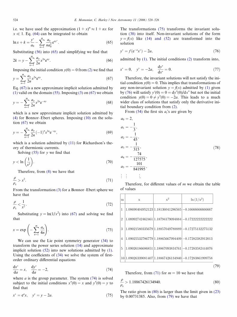
Therefore, for different values of m we obtain the tableof values

ð79ÞTherefore, from (71) for m = 10 we have that

qqc

> 1:18867426134940. ð80Þ

The ratio given in (80) is larger than the limit given in (23)by 0.00731385. Also, from (79) we have that

E. Momoniat, C. Harley / New Astronomy 11 (2006) 520–526 525

x < 1:091 ð81Þand therefore from (8) we have that

r < 1:091K

4pGqc

� �1=2

. ð82Þ

The solution (67) is computationally more expensivethan computing the power series solution (14). By specify-ing x we end up having to solve a nonlinear equation. Thiscomplication is somewhat simplified if we consider (67) as apolynomial in x, where x is the value to be calculated wheny is specified. A possible algorithm would read as follows:discretize the interval y 2 [0, �0.172839] where the bound-ary value 0 comes from (2) and �0.172839 is obtained from(79). We specify a y = yp value from the interval. We thenhave to solve the following polynomial equation for x = xp:Xm

n¼1

an

2nx2n

p enyp � yp ¼ 0. ð83Þ

Expanding (83) we find that

a1

2x2

peyp þ a2

4x4

pe2yp þ a3

6x6

pe3yp þ � � � þ am

2mx2memyp � yp ¼ 0.

ð84ÞSolving the nonlinear Eq. (84) using MATHEMATICA weobtain rapid convergence to the solution. In Fig. 1 we havetaken m = 14.

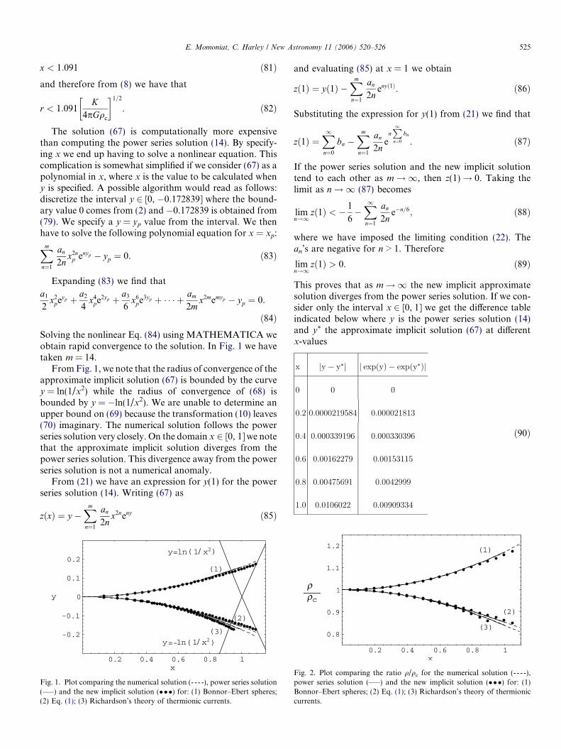
From Fig. 1, we note that the radius of convergence of theapproximate implicit solution (67) is bounded by the curvey = ln(1/x2) while the radius of convergence of (68) isbounded by y = �ln(1/x2). We are unable to determine anupper bound on (69) because the transformation (10) leaves(70) imaginary. The numerical solution follows the powerseries solution very closely. On the domain x 2 [0, 1] we notethat the approximate implicit solution diverges from thepower series solution. This divergence away from the powerseries solution is not a numerical anomaly.

From (21) we have an expression for y(1) for the powerseries solution (14). Writing (67) as

zðxÞ ¼ y �Xm

n¼1

an

2nx2neny ð85Þ

Fig. 1. Plot comparing the numerical solution (- - - -), power series solution(–––) and the new implicit solution (���) for: (1) Bonnor–Ebert spheres;(2) Eq. (1); (3) Richardson’s theory of thermionic currents.

and evaluating (85) at x = 1 we obtain

zð1Þ ¼ yð1Þ �Xm

n¼1

an

2nenyð1Þ. ð86Þ

Substituting the expression for y(1) from (21) we find that

zð1Þ ¼X1n¼0

bn �Xm

n¼1

an

2ne

nP1n¼0

bn

. ð87Þ

If the power series solution and the new implicit solutiontend to each other as m!1, then z(1)! 0. Taking thelimit as n!1 (87) becomes

limn!1

zð1Þ < � 1

6�X1n¼1

an

2ne�n=6; ð88Þ

where we have imposed the limiting condition (22). Thean’s are negative for n > 1. Therefore

limn!1

zð1Þ > 0. ð89Þ

This proves that as m!1 the new implicit approximatesolution diverges from the power series solution. If we con-sider only the interval x 2 [0, 1] we get the difference tableindicated below where y is the power series solution (14)and y* the approximate implicit solution (67) at differentx-values

ð90Þ

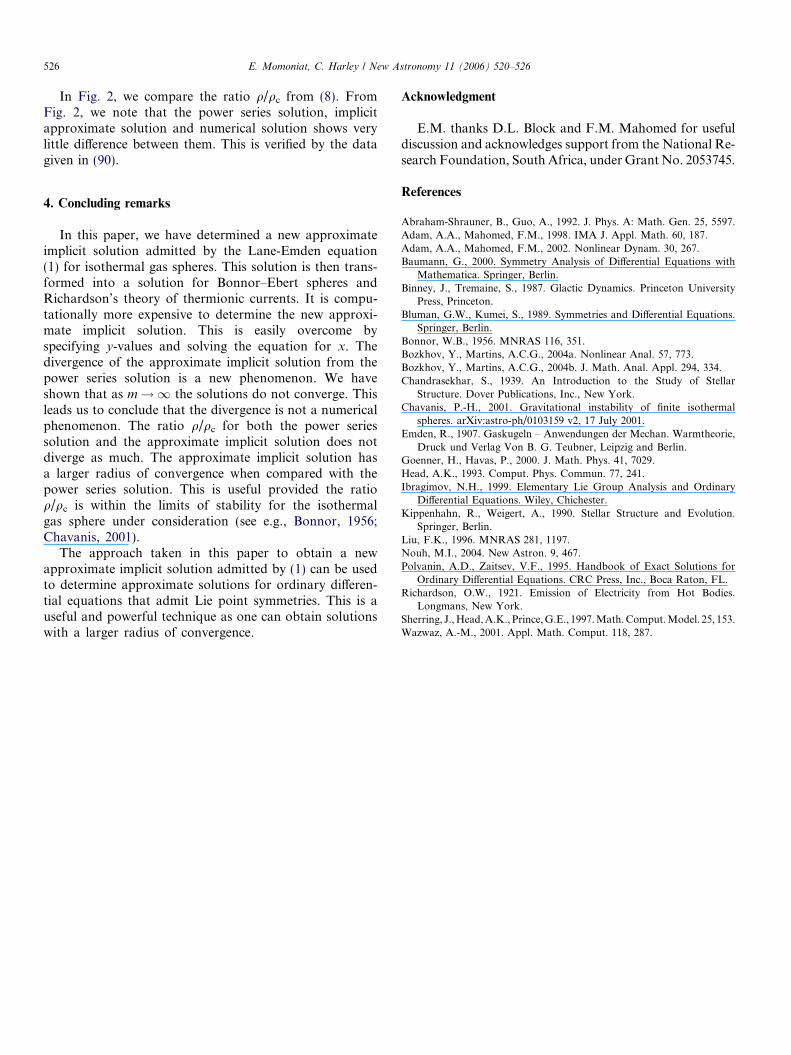
Fig. 2. Plot comparing the ratio q/qc for the numerical solution (- - - -),power series solution (–––) and the new implicit solution (���) for: (1)Bonnor–Ebert spheres; (2) Eq. (1); (3) Richardson’s theory of thermioniccurrents.

526 E. Momoniat, C. Harley / New Astronomy 11 (2006) 520–526

In Fig. 2, we compare the ratio q/qc from (8). FromFig. 2, we note that the power series solution, implicitapproximate solution and numerical solution shows verylittle difference between them. This is verified by the datagiven in (90).

4. Concluding remarks

In this paper, we have determined a new approximateimplicit solution admitted by the Lane-Emden equation(1) for isothermal gas spheres. This solution is then trans-formed into a solution for Bonnor–Ebert spheres andRichardson’s theory of thermionic currents. It is compu-tationally more expensive to determine the new approxi-mate implicit solution. This is easily overcome byspecifying y-values and solving the equation for x. Thedivergence of the approximate implicit solution from thepower series solution is a new phenomenon. We haveshown that as m!1 the solutions do not converge. Thisleads us to conclude that the divergence is not a numericalphenomenon. The ratio q/qc for both the power seriessolution and the approximate implicit solution does notdiverge as much. The approximate implicit solution hasa larger radius of convergence when compared with thepower series solution. This is useful provided the ratioq/qc is within the limits of stability for the isothermalgas sphere under consideration (see e.g., Bonnor, 1956;Chavanis, 2001).

The approach taken in this paper to obtain a newapproximate implicit solution admitted by (1) can be usedto determine approximate solutions for ordinary differen-tial equations that admit Lie point symmetries. This is auseful and powerful technique as one can obtain solutionswith a larger radius of convergence.

Acknowledgment

E.M. thanks D.L. Block and F.M. Mahomed for usefuldiscussion and acknowledges support from the National Re-search Foundation, South Africa, under Grant No. 2053745.

References

Abraham-Shrauner, B., Guo, A., 1992. J. Phys. A: Math. Gen. 25, 5597.Adam, A.A., Mahomed, F.M., 1998. IMA J. Appl. Math. 60, 187.Adam, A.A., Mahomed, F.M., 2002. Nonlinear Dynam. 30, 267.Baumann, G., 2000. Symmetry Analysis of Differential Equations with

Mathematica. Springer, Berlin.Binney, J., Tremaine, S., 1987. Glactic Dynamics. Princeton University

Press, Princeton.Bluman, G.W., Kumei, S., 1989. Symmetries and Differential Equations.

Springer, Berlin.Bonnor, W.B., 1956. MNRAS 116, 351.Bozkhov, Y., Martins, A.C.G., 2004a. Nonlinear Anal. 57, 773.Bozkhov, Y., Martins, A.C.G., 2004b. J. Math. Anal. Appl. 294, 334.Chandrasekhar, S., 1939. An Introduction to the Study of Stellar

Structure. Dover Publications, Inc., New York.Chavanis, P.-H., 2001. Gravitational instability of finite isothermal

spheres. arXiv:astro-ph/0103159 v2, 17 July 2001.Emden, R., 1907. Gaskugeln – Anwendungen der Mechan. Warmtheorie,

Druck und Verlag Von B. G. Teubner, Leipzig and Berlin.Goenner, H., Havas, P., 2000. J. Math. Phys. 41, 7029.Head, A.K., 1993. Comput. Phys. Commun. 77, 241.Ibragimov, N.H., 1999. Elementary Lie Group Analysis and Ordinary

Differential Equations. Wiley, Chichester.Kippenhahn, R., Weigert, A., 1990. Stellar Structure and Evolution.

Springer, Berlin.Liu, F.K., 1996. MNRAS 281, 1197.Nouh, M.I., 2004. New Astron. 9, 467.Polyanin, A.D., Zaitsev, V.F., 1995. Handbook of Exact Solutions for

Ordinary Differential Equations. CRC Press, Inc., Boca Raton, FL.Richardson, O.W., 1921. Emission of Electricity from Hot Bodies.

Longmans, New York.Sherring, J., Head, A.K., Prince, G.E., 1997. Math. Comput. Model. 25, 153.Wazwaz, A.-M., 2001. Appl. Math. Comput. 118, 287.